dynamic(modelling(of compliant moored&submerged& systems ... ·...
TRANSCRIPT

1
Proceedings of the 2nd Marine Energy Technology Symposium METS2014
April 15-‐18, 2014, Seattle, WA
DYNAMIC MODELLING OF COMPLIANT-‐MOORED SUBMERGED SYSTEMS WITH APPLICATIONS TO MARINE ENERGY CONVERTERS
Tyler Nichol1 Northwest National Marine Renewable Energy Center University of Washington Seattle, Washington, USA
Geoff DuBuque Northwest National Marine Renewable Energy Center University of Washington Seattle, Washington, USA
Brian Fabien Northwest National Marine Renewable Energy Center University of Washington Seattle, Washington, USA
1Corresponding author: [email protected] ABSTRACT This paper presents a full-‐range-‐of-‐motion numerical model of the dynamic characteristics of compliant-‐moored submerged systems in unsteady fluid flow using a first-‐principles approach. The program, implemented using the MATLAB software package, is in development with the primary intention of being applicable to in-‐stream hydrokinetic turbines, though many wave energy converter and offshore wind turbine platform systems will also be capable of being modeled. A Lagrangian frame of reference is adopted to generate the equations of motion of a given system. The external forces presently considered in the model are those of gravity, buoyancy, and fluid drag, with plans to include more sophisticated fluid effects as the project advances. The development of the kinematic system and the body drag model are discussed. Additionally, two validation tests are presented. The results of the validation tests provide confidence that the methods employed have the potential to realistically simulate the dynamic behavior of compliant-‐moored systems once more detailed effects of fluid loading are accounted for. INTRODUCTION Tidal power devices harness the kinetic energy in tidally driven currents for electricity generation. Tidal turbines are analogous to wind turbines and share a number of engineering features. Most designs for tidal turbines incorporate a rigid mounting structure which is either pile-‐driven into the seabed [1] or is designed such that gravitational forces keep the structure upright when subjected to high currents [2]. Pile-‐supported turbines are typically feasible in water depths up to 40 𝑚. For gravity foundations, the
weight required to resist overturning limits hub heights to the less energetic portion of the water column. Additionally, both of these strategies place specific requirements on the vessels used for installation and recovery, adding to the overall engineering challenge and expense of such projects. A mooring concept that combines the ease of deployment of gravity platforms with the advantageous hub heights of pile structures is to design buoyancy into the turbine and fix it to the seafloor via flexible mooring lines attached to an anchor or installed foundation. As an added benefit, compliant-‐moored turbines could potentially introduce fewer environmental stressors. Boehlert and Gill [3] suggest that the greatest impact due to the introduction of manmade devices into the marine environment is on benthic habitats and ecosystems. Compliant-‐moored turbines allow for less hard substrate to be placed into the marine environment, reducing the magnitude of the modification to the structural habitat and the changes in water circulation and currents. Additionally, as evidenced by an environmental appraisal for the Argyll Tidal Energy Demonstrator Project [4], mooring configurations can be designed such that the only direct impact to benthic communities is localized at the mooring foundations. This method has the advantage of enabling turbine operation in deep water while occupying the energetic flows occurring higher up in the water column. Designing for the uplift force experienced by the mooring foundations in a compliant-‐moored turbine system is likely a simpler engineering challenge when compared to the overturning moment induced onto a rigidly-‐supported turbine operating at a comparable water depth and hub height. Additionally, compliant-‐moored devices may offer benefits to
2
the ease and cost of deployment and recovery of the device when compared to pile-‐driven or gravity foundation methods. To assist in the design of single or arrays of compliant-‐moored tidal turbines, NNMREC is developing a software tool to simulate mooring performance. This consists of a numerical simulation implemented in MATLAB (www.mathworks.com) of a moored turbine system which, when given the necessary input parameters, models the dynamic response of the system to a specified flow field. This information will help turbine developers determine the best configuration of turbines and mooring lines to maintain the optimal turbine orientation to the fluid flow and position in the water column while staying within structural loading and mooring foundation uplift limits. Furthermore, this tool will be helpful in the design of active or passive control systems to optimize turbine position, as the performance of various control techniques and parameters can be evaluated computationally, reducing the overall effort and expense associated with field testing. The methods described herein were developed primarily with consideration to moored tidal turbines, though they will eventually be expanded to include effects relevant to the analysis of wave energy converters or offshore wind platforms. BACKGROUND Within the growing field of tidal energy harvesting, compliant moored devices have often been mentioned as a potential area for investigation [2,5,6]. The Energy Systems Research Unit (ESRU) at the University of Strathclyde is developing a device that employs a single mooring line anchored to the sea floor and tensioned using a buoy that may or may not be surface-‐penetrating, with a neutrally buoyant tidal turbine attached to the line at some point along its length [7]. The turbine features two sets of blades rotating in opposite directions to eliminate the reactive torque generated by the rotating turbine blades. This device has undergone successful testing at sea in an energetic ocean current and ESRU is currently working on up-‐scaling and long-‐term reliability testing of the device. A second project is being led by Ocean Renewable Power Company (ORPC). Named the OCGen Power System, it consists of an array of helical cross-‐flow turbines which resemble vertical axis wind turbines. The turbines are held in place on the seafloor by a system of mooring lines. Because of the reduced construction effort required to anchor the mooring lines as compared to installing rigid support structures in the
seafloor, the OCGen is suitable for deployment in water depths surpassing 80 𝑚 [8]. The development of these systems could be supported by a time-‐domain dynamic model. Clark et al [7] discuss the importance of predicting instabilities in a compliant-‐moored system to achieve optimal performance. Different mechanisms for dealing with instabilities can be evaluated using an accurate dynamic model before experimental methods are employed, thereby allowing a wide range of options to be investigated in a short period of time and using minimal resources. There are currently several options for software packages capable of performing dynamic analysis on moored tidal energy systems. One of these is OrcaFlex (www.orcina.com), a time-‐domain numerical solver which is widely used in many marine engineering industries to perform dynamic analysis of offshore marine systems. OrcaFlex was used by Columbia Power Technologies, LLC (CPT), to aid in the design of a wave energy converter [9]. The software was used to evaluate significant design changes to the device in terms of performance in a relatively low-‐cost and low-‐impact manner. They found that, due to the specific nature of ocean energy harvesting devices, off-‐the-‐shelf software packages often need to be supplemented with custom-‐made numerical approaches [9]. To accurately model the system, CPT worked with Garrad Hassan and Partners (GH) to develop a numerical modelling package suited to their applications. Through implementation of the GH Wavefarmer software to examine frequency-‐domain behavior, and importing terms obtained from the frequency-‐domain modelling into OrcaFlex , they were able to generate a model for the mooring behavior of a WEC which closely resembled experimental results from data collected from a 1/33 scale test device [9]. Another fully dynamic, time-‐domain hydrodynamic simulator was developed by Dynamic Systems Analysis, Ltd. ProteusDS (www.dsa-‐ltd.ca) specializes in underwater cable dynamics and can model systems consisting of both rigid bodies and flexible cables and nets by employing finite-‐element discretization of flexible members and a nonlinear hydrodynamic cable model. This program was used by Hall et al. [10] to model the dynamic behavior of floating offshore wind turbines through coupling with a quasi-‐static aero-‐hydro simulator called FAST (wind.nrel.gov/designcodes/simulators/fast), which uses Blade-‐Element-‐Momentum Theory and linear hydrodynamics to describe a floating wind turbine device [11]. In addition, FAST includes a quasi-‐static model of taut or slack
3
mooring lines by solving a system of analytical catenary cable equations to find the static-‐equilibrium position and tension of the lines. The linear hydrodynamics simulator WAMIT (www.wamit.com) was used to model the hydrodynamic loads on the floating wind turbine platform. Coupling of FAST with ProteusDS yields a fully dynamic finite element model of floating wind turbine system dynamics. The static-‐equivalent results from the dynamic model of a floating offshore wind turbine were compared to results found using FAST’s default quasi-‐static mooring model, and the two were found to be in good agreement [10]. Further testing involving irregular sea states that cause the motions of the floating platform and surface waves to be out of sync will reveal a more complete picture of the differences between the fully-‐dynamic model and the quasi-‐static model. Though these software packages have been shown to be applicable to marine energy systems with good accuracy, the development of a new, first-‐principles code is justified by the following: 1) Code can be developed for specific functionalities and readily expanded to include secondary effects or to accept different formats of system parameter inputs (for example, one might express fluid velocity as a function of time and space or as a velocity vector field). 2) The simulation is developed from the ground up with the goal of modeling mooring dynamics specifically for marine energy converters. This will hopefully offer benefits over commercial software packages in terms of the ease and completeness with which a compliant-‐moored MEC system can be fully defined and parameterized, making this simulation better-‐suited to rapid-‐iteration design where many different system configurations may need to be examined. 3) Total control over both how the model is constructed and how the solution is obtained allows for greater confidence in the results. 4) Greater flexibility when integrating with other computational tools such as active control system simulators. METHODS
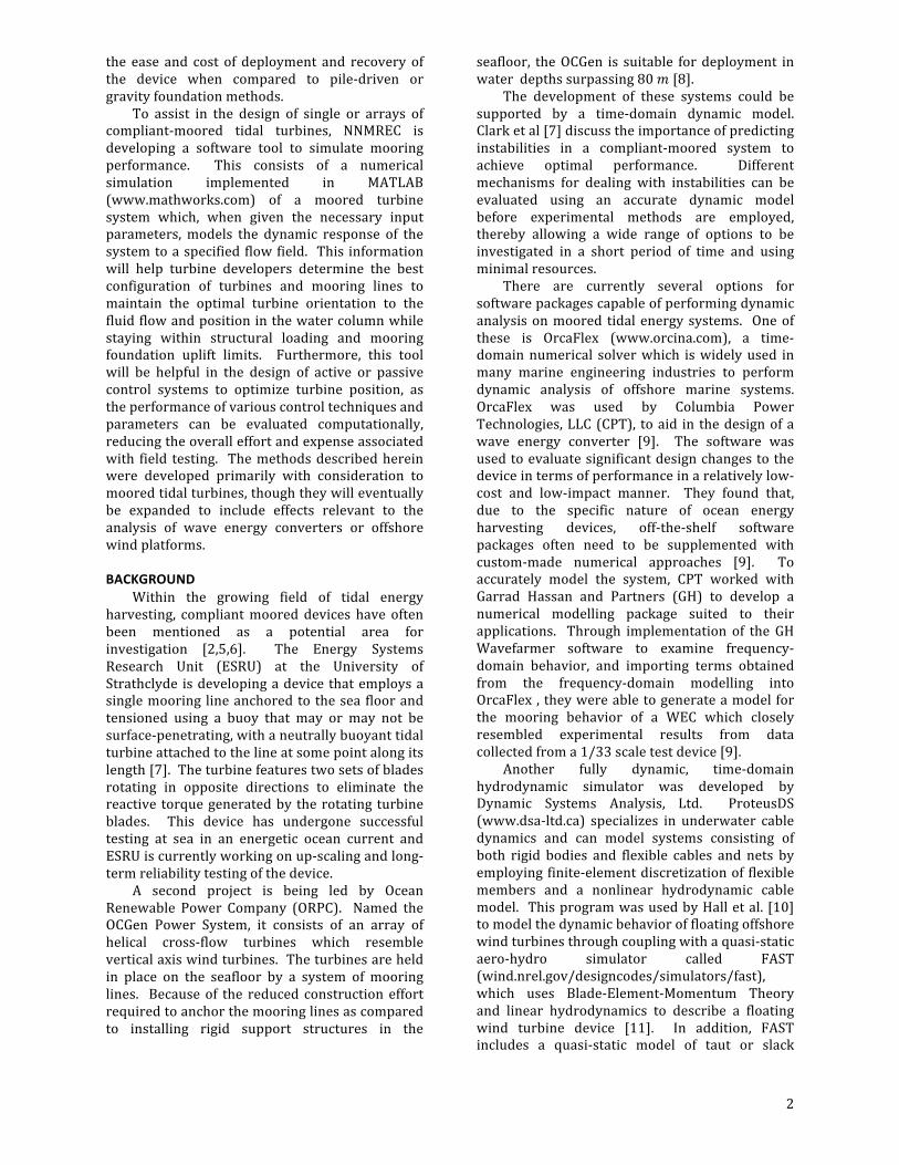
FIGURE 1: SAMPLE COMPLIANT-‐MOORED SYSTEM
A sample compliant-‐moored tidal turbine system that can be modeled using the described techniques is that shown in Figure 1. These systems can contain multiple rigid bodies connected via mooring lines to the sea floor or to other bodies. Multiple bodies can also be joined rigidly such that one body is constrained to a fixed position within a free body’s coordinate frame. Any one body in a rigid grouping can be defined arbitrarily as the free body. The constrained body does not add to the number of degrees of freedom of the system, whereas each free body adds six DOF. A free node is used to connect multiple mooring lines at a junction and adds three translational DOF. A system can be composed of as many or as few free bodies, constrained bodies, free nodes, and mooring lines as necessary to describe the system. Mooring lines are modeled using a finite segment approach. Each line is divided into a number of discreet segments specified by the user during configuration of the system. The greater the number of segments, the more closely the model will resemble a continuous mooring line until a point where the number of segments is so great that the length of each segment is on the same order of magnitude as the computer’s floating point precision and rounding errors begin to dominate. Each additional line segment also introduces three additional DOF to the system, which increases the computation time required to converge on a solution. An appropriate balance must be found between a sufficiently realistic model and one that can be solved in a reasonable amount of time. To analyze the dynamic behavior of these systems, it is necessary to develop expressions for all forces acting on the system as functions of the position and velocity of each feature. Due to the complex geometry of a tidal turbine, the fluid forces and the fluid-‐structure interactions are difficult to model. These effects are simplified to allow for initial development of the computational methods. This approach allows for the development of the program to a point where the governing equations can be derived and solved for using a reasonable approximation of fluid forces for simple geometries and light loading, however for the model to accurately simulate tidal turbine behavior in a sufficiently wide range of operating conditions, more advanced calculations of the fluid forces will be needed. Presently, all bodies in a system, including the turbines themselves, are modeled as simple rigid bodies. It is assumed that the component of fluid velocity parallel to a body-‐fixed axis imparts a drag force which is parallel to that axis, i.e. no lift. The lift experienced by symmetric bodies at non-‐
4
zero angles of attack is approximated by decomposing the relative fluid velocity into its components along the body-‐fixed axes and using corresponding drag coefficients and characteristic areas for flow along each coordinate direction. This approach is suitable for blunt body geometries, assuming the flow possesses a sufficiently high Reynolds number. Rigid Body and Mooring Line Dynamics A complete model will result in a system of differential equations of motion in the familiar form of Equation (1), where 𝑀 is a mass matrix, 𝐵 is a damping coefficient matrix (if external damping is applied), 𝐾 is a stiffness matrix, and 𝐹 is an array of forces acting on the corresponding displacement variable consisting of the contributions from drag, gravity, buoyancy, applied forces, and any other included forces.
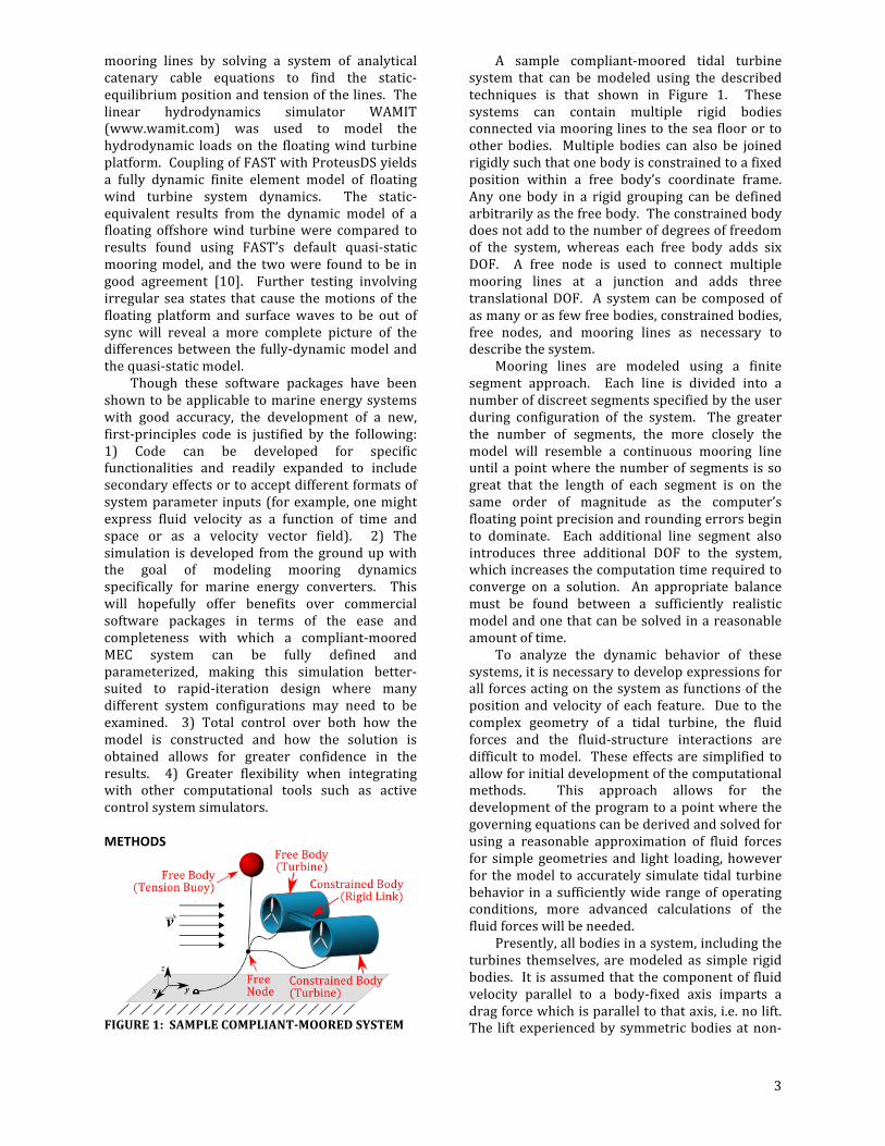
𝑀𝑥 + 𝐵𝑥 + 𝐾𝑥 = 𝐹 𝑥, 𝑥, 𝑡 (1) Figure 2 shows the free-‐body diagram of a rigid body within a simply configured system and Figure 3 shows the forces acting on an individual line node. It should be noted that slack line conditions are not yet handled by the simulation. Any instantaneous line segment length that is less than the natural length of the segment will result in compressive spring forces which do not occur in physical mooring lines. Until slack line conditions are incorporated into the model, it will only be useful for taught moorings. The number of equations in the system is equal to the number of degrees of freedom, which is determined by the number of rigid bodies, free nodes, and mooring line segments. Rather than attempting to assemble the system of differential equations into a form similar to Equation (1) directly, the program implements Lagrange’s equation of motion, given as Equation (2), to derive the equations of motion for each independent displacement variable.
𝑑𝑑𝑡𝜕𝑇𝜕𝑞!
−𝜕𝑇𝜕𝑞!
+𝜕𝑉𝜕𝑞!
+𝜕𝐷𝜕𝑞!
= 𝑒! (2)
𝑇, 𝑉, and 𝐷 are scalar symbolic expressions for the total kinetic energy, the total potential energy, and the rate of energy dissipated due to linear damping terms, respectively; 𝑞 and 𝑞 are the symbolic arrays of displacement and velocity variables, respectively, and 𝑒 is an array containing symbolic expressions for the forces acting on each independent displacement variable. The symbolic expressions for 𝑇 , 𝑉 , 𝐷 , and each entry in 𝑒 are non-‐linear functions of 𝑞, 𝑞, and 𝑡. The differentiations needed to implement
Lagrange’s equation are performed using commands from the MATLAB Symbolic Toolbox.
FIGURE 2. RIGID BODY KINEMATIC SYSTEM.
FIGURE 3. LINE SEGMENT KINEMATIC SYSTEM.
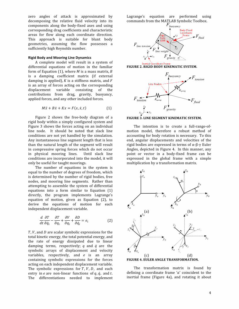
The intention is to create a full-‐range-‐of-‐motion model, therefore a robust method of accounting for body rotation is necessary. To this end, angular displacements and velocities of the rigid bodies are expressed in terms of α-‐β-‐γ Euler Angles, depicted in Figure 4. In this manner, any point or vector in a body-‐fixed frame can be expressed in the global frame with a simple multiplication by a transformation matrix.
(a) (b)
(c) (d)
FIGURE 4. EULER ANGLE TRANSFORMATION.
The transformation matrix is found by defining a coordinate frame ‘𝑎’ coincident to the inertial frame (Figure 4a), and rotating it about

5
the 𝑥!-‐axis by an angle 𝛼 to frame ‘𝑏’ (Figure 4b). Frame ‘𝑏’ is then rotated by an angle 𝛽 about the 𝑦!-‐axis to frame ‘𝑐’, which is then rotated about the 𝑧!-‐axis by the angle 𝛾 to obtain the body-‐fixed frame ‘1’. Each individual step is accomplished in sequence through multiplication with a single transformation matrix. The product of the matrices for each step yields the transformation matrix to express any point or vector in the body-‐fixed frame in terms of the inertial frame, as described in Equation (3) [12]. 𝐴
=1 0 00 𝑐! −𝑠!0 𝑠! 𝑐!
𝑐! 0 𝑠!0 1 0−𝑠! 0 𝑐!
𝑐! −𝑠! 0𝑠! 𝑐! 00 0 1
=𝑐!𝑐! −𝑐!𝑠! 𝑠!
𝑠!𝑠!𝑐! + 𝑐!𝑠! −𝑠!𝑠!𝑠! + 𝑐!𝑐! −𝑠!𝑐!−𝑐!𝑠!𝑐! + 𝑠!𝑠! 𝑐!𝑠!𝑠! + 𝑠!𝑐! 𝑐!𝑐!
.
(3)
A vector expressed in a body-‐fixed frame 𝑟! is found in terms of the inertial frame 𝑟! as shown by Equation (4).
𝑟! = 𝐴! 𝑟! (4) Additionally, a point 𝑃 in a body-‐fixed frame whose origin is not coincident with that of the inertial frame can be found by application of Equation (5).
𝑃! = 𝑃!! + 𝐴! 𝑃! (5) 𝑃!! is the location of the origin of the body-‐fixed frame ‘1’ with respect to the inertial frame ‘0’, 𝑃! is the location of point 𝑃 with respect to the body-‐fixed frame, and 𝑃! is the location of point 𝑃 expressed in the inertial frame. The angular velocity of the body-‐fixed frame can be written in terms of the time derivative of a body’s Euler Angles as Equation (6).
𝜔! = 𝛼𝚤! + 𝛽𝚥! + 𝛾𝑘! (6) where 𝚤! , 𝚥! , and 𝑘! are the unit vectors along the 𝑥! , 𝑦! , and 𝑧! axes, respectively. Noting that the 𝑥! axis is parallel to the inertial 𝑥-‐axis, the unit vector 𝚤! is also parallel to the global 𝚤! unit vector, therefore 𝚤! = 𝚤! = 𝑐!𝑐!𝚤! − 𝑐!𝑠!𝚥! + 𝑠!𝑘! . With similar observations about the 𝚥! and 𝑘! unit vectors, the resultant angular velocity of a rigid body is expressed in terms of the time derivative of its Euler Angles as shown in Equation (7).
𝜔! =𝑐!𝑐! 𝑠! 0−𝑐!𝑠! 𝑐! 0𝑠! 0 1
𝛼𝛽𝛾. (7)
The velocity of any fixed point in a body-‐fixed frame can be expressed in terms of the inertial coordinate system as Equation (8).
𝑣! = 𝑣!! + 𝐴! 𝜔! × 𝑃! (8) where 𝑣!! is the velocity of the origin of the body-‐fixed frame ‘1’ with respect to the inertial frame and 𝑃! is the location of the body-‐fixed point 𝑃 with respect to the body-‐fixed frame. Using Euler Angle transformations facilitates the derivation of the symbolic expressions for the kinetic and potential energies in the system as well as the rate of energy dissipated due to applied damping terms and the resultant total force due to gravity, buoyancy, and fluid and applied forces. Kinetic and Potential Energy To derive the equations of motion using Lagrange’s equation, an expression for the total kinetic energy as a function of the independent variables is needed. The total kinetic energy is the sum of the kinetic energies of all individual mass-‐possessing elements of the system. The general equation for the kinetic energy of a body is 𝑇!"#$,! =
!!𝑚! 𝑣!! + 𝑣!! + 𝑣!! + 𝐼!,!𝜔!!
+ 𝐼!,!𝜔!! + 𝐼!,!𝜔!! (9)
where 𝑚 is the mass of the object, 𝑣! , 𝑣! , and 𝑣! are the components of velocity in the inertial x, y, and z directions, 𝐼!,! , 𝐼!,! , and 𝐼!,! are the body’s mass moment of inertia about the body-‐fixed axes, and 𝜔! , 𝜔! , and 𝜔! are the body’s components of angular velocity about the instantaneous body-‐fixed axes as found from Equation (7). Using the lumped-‐parameter approach for the mooring lines, the kinetic energy for each line is found as the sum of the individual kinetic energies of each lumped mass. Rotational kinetic energy of line nodes is expected to be small and therefore is neglected. The end-‐nodes of a mooring line are fixed to other features and do not constitute independent displacement variables, therefore the velocity of these nodes is represented in the symbolic expression for kinetic energy as a function of the displacement variables belonging to the feature to which the end-‐node is fixed. Potential energy is stored in the elastic mooring lines. Gravitational effects are not included in the expression for system potential energy because they are accounted for in the

6
model as forces acting on the system. The quantity of potential energy stored in each segment is
𝑉!"#$"%&,! =!!𝑘! ℓ𝓁! − ℓ𝓁!,!
! (10)
where 𝑘! is the segment spring constant, ℓ𝓁! is the instantaneous segment length, and ℓ𝓁!,! is the un-‐stretched segment length. The instantaneous segment length is found symbolically as a function of the system’s independent displacement variables. The total system potential energy is calculated as the sum of the potential energies stored in each individual discretized mooring line segment. Fluid Force Model One of the greatest challenges of this project is the calculation of fluid forces acting on the system. At this stage of development, fluid forces are approximated component-‐wise as pure drag; that is, a given body will be subjected to drag forces calculated along its body-‐fixed axes, and a given line segment will be subjected to drag acting tangent and normal to its axis. Modelling the drag forces on rigid bodies begins with finding the velocity of the fluid relative to the instantaneous velocity of the body. This relative velocity is then transformed to the body-‐fixed coordinate frame using the Euler Angle transformations described earlier. From here, the drag force vector with respect to the body-‐fixed frame can be calculated using Equation (11).
𝐹!"#$,! =!!𝜌!𝐶!,!𝔸!𝑢! 𝑢! (11)
where 𝐶!,! , 𝔸! , and 𝑢! are the coefficient of drag, characteristic area, and relative fluid velocity, respectively, with respect to the body-‐fixed coordinate 𝑖 -‐direction, such that the total drag force vector is expressed as 𝐹! !"#$ = 𝐹!"#$,!! 𝐹!"#$,!! 𝐹!"#$,!! ! .
Figure 5 demonstrates in two-‐dimensions how drag forces are decomposed into axis-‐aligned components and applied to a rigid body. In this figure, 𝑣! is the velocity of the fluid relative to the rigid body along the global 𝑦!-‐axis, 𝑣! and 𝑤! are the relative fluid velocities aligned to the body-‐fixed 𝑦! and 𝑧! axes, respectively, 𝐴!! and 𝐴!! are the body characteristic areas corresponding to flow along the 𝑦! and 𝑧! axes, respectively, and 𝐶!,!! and 𝐶!,!! are the coefficients of drag for fluid flow along the corresponding body-‐fixed axis. Note that for geometries such as a cube or a sphere where the values for the coefficients of drag and the characteristic areas are equivalent
along each direction, the resultant drag force vector will always act parallel to the relative fluid flow regardless of body orientation. The force is then expressed back in terms of the inertial coordinate frame by another operation with the transformation matrix.
FIGURE 5. DECOMPOSITION OF DRAG FORCE ACTING ON A RIGID BODY.
The drag forces acting on the mooring lines are handled in a slightly different manner. Because the mooring line segments more closely resemble elongated cylinders rather than bluff bodies, the drag force experienced by a line segment is calculated as the vector sum of a tangential and normal force component. The characteristic area used for calculating the tangential force component is the cylindrical surface area of the line segment, 𝔸 = 𝜋𝑑ℓ𝓁, where 𝑑 is the line diameter (assumed to be constant under load) and ℓ𝓁 is the instantaneous length of the line segment. For calculating the normal drag force component, the lengthwise projected area, 𝔸 = 𝑑ℓ𝓁, is used. The tangential force component acts along a vector parallel to the line segment, whereas the normal force acts along a vector normal to the segment and in the plane created by the relative fluid velocity vector and the axis of the line segment, as shown in Figure 6. For mooring lines with more complex geometries such as chains, whose segments do not resemble elongated cylinders, suitable equivalent parameter values are used. Using a lumped-‐parameter approach, the drag force on a line segment is calculated as though it is acting through the geometric center of the segment and then distributed evenly between the two adjacent line nodes.
FIGURE 6. DECOMPOSITION OF DRAG FORCE ACTING ON AN IDIVIDUAL LINE ELEMENT.

7
Seafloor Constraint The normal force exerted by the seafloor is modeled by a non-‐linear force applied to each z-‐displacement variable. The empirical form of the model is
𝐹!"#$%&&' =𝜂𝑧!!
𝑘 (12)
where 𝜂 is a tuning variable and 𝑧! is the distance from the seafloor. In this way, the force is only significant when the displacement variable accounting for the z-‐position of a line node, free node, or rigid body is close to zero. The appropriate value of 𝜂 depends on the length, mass, and number of discretized segments for a mooring line. This quantity should be chosen such that the normal force acting on the mooring line nodes due to the seafloor is in equilibrium with gravitational forces at an acceptably small distance from the seafloor. Larger values for 𝜂 will cause the line to come to rest at unrealistically large distances from the seafloor, and values that are too small can lead to non-‐convergence as the distance approaches zero. For a system with a submerged line segment weight equivalent to 1.5 kilograms, a value of 𝜂 = 10!! 𝑁𝑚! produced realistic results. This method does not take into consideration the physical dimensions of a rigid body. It is assumed that the desired information is whether a structural body collides with the seafloor or not, rather than how the system responds when it does. On the other hand, the response of a system with mooring-‐line interaction with the seafloor is of interest, and this model gives a reasonable representation of mooring-‐lines lying partially on the seafloor. Once the expressions for kinetic energy, potential energy, rate of energy dissipation, and the combined force loading are obtained, Lagrange’s Equation of Motion is implemented to generate the complete system of differential equations which describes the system. This system is then solved numerically using the built-‐in MATLAB function ode15i.m, which outputs the value for each displacement variable at a given time within the user defined interval. PRELIMINARY MODEL VALIDATION TESTS Comparison to steady-‐state model The first benchmark test evaluates the equilibrium position of a potential tidal turbine system. The results obtained by running the dynamic model until a steady-‐state condition is reached are compared to results of an equilibrium model developed by DuBuque [13], who presents
a numerical method to obtain the equilibrium position of a tidal turbine in a steady fluid flow through iterative minimization of the potential energy of the system. The system configuration selected is shown in Figure 7.
FIGURE 7. SYSTEM SCHEMATIC FOR COMPARISON TO STATIC-‐EQUILIBRIUM MODEL.
This system is composed of a single rigid body with four mooring lines in a fluid with density 𝜌 = 1020 𝑘𝑔 𝑚! moving with a constant velocity of 4 𝑚/𝑠 . The body measures 28 𝑚 wide, 4 𝑚 deep, and 8.5 𝑚 tall. Due to the fact that this body represents a tidal turbine which allows some fluid to pass through its volume, the effective surface areas of the body are only a small percentage of the total rectangular surface area. The rigid body properties for this system are given in Table 1. TABLE 1. RIGID BODY PROPERTIES – STATIC MODEL COMPARISON TEST.
Property Value Mass: 𝑚 = 5000 𝑘𝑔 Mass Moment of Inertia:
𝐼 = 𝐼!! 𝐼!! 𝐼!!= 4 4 4 𝑘𝑔 𝑚!
Volume: 𝑉 = 10 𝑚! Initial position in global frame:
𝑌! = 𝑥! 𝑦! 𝑧!= 0 0 20 𝑚
Initial orientation in global frame:
𝜃! = 𝛼! 𝛽! 𝛾!= 0 0 0 𝑟𝑎𝑑
Effective Surface Area:
𝐴 = 𝐴!! 𝐴!! 𝐴!!= 16 24 11 𝑚!
Coefficients of drag:
𝐶! = 𝐶!,!! 𝐶!,!! 𝐶!,!!= 0.5 0.5 0.5
The mooring line stiffness is based on a material with a Young’s modulus of 10 GPa and a diameter of 5 cm. The resulting unit spring constant is found as described in Equation (13).

8
𝑘!"#$ = 𝐸𝐴 = 10𝑥10! 𝑁 𝑚!
𝜋40.05 𝑚 !
= 19635000 𝑁 𝑚 𝑚 (13)
This is the spring constant for a line 1 meter in length. The program uses this value to calculate the spring constant for each line segment based on the length of each segment, which is determined by the overall length of the mooring line and the number of segments into which it is divided as stipulated by the user. The remaining mooring line properties are presented in Table 2. TABLE 2. MOORING LINE PROPERTIES – STATIC MODEL COMPARISON TEST.
Property Value Linear mass: 𝑚 = 10 𝑘𝑔 𝑚 Diameter: 𝑑 = 0.05 𝑚 Length: 𝐿 = 44 𝑚 Unit stiffness: 𝑘!"#$ = 19635000 𝑁 𝑚 𝑚 Coefficients of drag:
𝐶! = 𝐶!,!"#$ 𝐶!,!"#= 1.0 0.3 𝑚
The simulation is run for a long enough duration such that the system reaches steady-‐state. The resulting equilibrium position and orientation of the rigid body are presented in Table 3, along with those observed by DuBuque for comparison.
TABLE 3. RESULTS OF STATIC MODEL COMPARISON TEST.
Position/ Orientation
Static Model [13]
Dynamic Model Error
𝑥 (𝑚) 10-‐5 0 0% 𝑦 (𝑚) 2.263 2.3864 5% 𝑧 (𝑚) 16.30 16.0411 1.6% 𝛼 𝑟𝑎𝑑 0.3809 0.3758 1.3% 𝛽 𝑟𝑎𝑑 10-‐6 0.0 0% 𝛾 𝑟𝑎𝑑 10-‐6 0.0 0%
The validity of the drag force model acting on a rigid body and mooring line system under steady state conditions is evidenced by the consistency between the static-‐equilibrium model and the static-‐equivalence obtained from the dynamic solution. Comparison to Analytical Solution to Mass-‐Spring-‐Damper System The first dynamic validation test is used to determine the efficacy of the automatic derivation and solution of the equations of motion of a system without consideration to the developed
fluid force model. For this test, a two degree of freedom mass-‐spring-‐damper system is modeled and the behavior as obtained from the numerical model is compared to the analytical solution to the governing equations of motion. The chosen test system is presented in Figure 8a. Careful attention must be paid to ensure that the system generated in the numerical model accurately resembles the chosen test system due to the fact that the numerical model expects all compliant lines to be continuous with uniform linear mass, whereas the test system utilizes ideal massless springs. Similarity is achieved in the numerical model by describing a system with a single mooring line discretized into two segments attached to a rigid body. By dividing the mooring line into only two segments, a single lumped-‐parameter line node is created which is analogous to mass 2 in the test system. The lumped-‐mass of the sole line node is equal to the mass of one line segment; additionally, a quantity of mass equal to one-‐half that of the line segment is lumped to the rigid body as part of the discretization scheme, therefore the linear mass of the mooring line and the mass of the rigid body must be chosen such that the resulting lumped-‐masses of the line node and rigid body are equal to the masses 𝑚! and 𝑚! in the test system, respectively. Additionally, the unit spring constant of the mooring lines must be chosen such that the resulting spring constant of each line segment is equal to the spring constant 𝑘 in the test system.
FIGURE 8. MASS-‐SPRING-‐DAMPER SYSTEM (a) AND EQUIVALENT NUMERICAL SYSTEM (b) FOR PRELIMINARY DYNAMIC VALIDATION TEST.
In the test system, the body mass 𝑚! and node mass 𝑚! are set to 100 𝑘𝑔 and 8 𝑘𝑔 respectively, the spring constants of both springs are set to 500 𝑁 𝑚 , and the damping constant is set to 10 𝑁𝑠 𝑚 . A sinusoidal force is applied as a function 𝐹 = −500𝑁 sin 2𝜋𝑡 10𝑠 . The governing equations of motion for this system are expressed as shown in Equations (14) and (15). 𝑚!𝑦! = −𝑚!𝑔 + 𝑘 𝑦! − 𝑦! − 5𝑚 − 𝑏𝑦!
− 500𝑁 sin 2𝜋𝑡 10𝑠 𝑚!𝑦! = −𝑚!𝑔 + 𝑘 5𝑚 − 𝑦!
− 𝑘 𝑦! − 𝑦! − 5𝑚
(14)
(15)

9
With the initial positions of each mass as shown in the figure and the initial velocities of both masses set to zero, this system of differential equations of motion is easily solved analytically using Mathematica to obtain the vertical position of masses 𝑚! and 𝑚! as functions of time. The corresponding system as modeled in the dynamic modeling program is shown in Figure 8b, where the mooring line is modeled as two discrete 4 meter segments. To match the test model, the unit spring constant is set to 𝑘!"#$ = 500 𝑁 𝑚 4𝑚 = 2000𝑁𝑚 𝑚 . The
linear mass is set to 2 𝑘𝑔 𝑚 such that the mass of the lumped-‐parameter node is 8 𝑘𝑔, and the mass of the rigid body is set to 96 𝑘𝑔 such that when the mass of half of a line segment is lumped to the body, the result is equal to 𝑚! . Because the damper in the test system acts between body 1 and the fixed inertial frame, its value is the same as that applied to the rigid body in the numerical model. The simulation is run several times while varying the value for the relative and absolute error tolerance applied to the ODE solver. Figure 9 shows the resulting maximum error between the solution (y-‐position of the mass as a function of time) obtained analytically and that found by the numerical simulation as a function of the solver tolerance. The figure demonstrates that as the tolerances are tightened on a logarithmic scale, the absolute error between the analytical and the numerical solutions also decreases logarithmically.
FIGURE 9. MAXIMUM ABSOLUTE ERROR AS A FUNCTION OF ODE SOLVER TOLERANCES.
This test serves to validate several key components of the program. It shows that the program is able to effectively extract the differential equations of motion of a system involving a mass, elastic cable, and damper. Additionally, the results prove that the ODE solver is capable of solving the equations of motion and producing a representation of the system behavior
with an accuracy dependent on the specified error tolerance. This test was conducted with only two discretized line segments so that an analytical solution to an equivalent system could easily be found. It is reasonable to conclude that similar results will be found as the number of line segments is increased when compared to the analytical solution to the corresponding mass-‐spring-‐damper system. Since finite segment theory states that a continuous line can be modeled as discretized segments (see [14]), these results support the claim that this model for mooring line dynamics accurately reflects the behavior of a mass tethered by a continuous mooring line with uniform linear mass and stiffness. What this test does not validate is the fluid forcing model, since fluid forces were not applied. FUTURE DEVELOPMENT AND APPLICATION A great deal of effort is still required to advance the dynamic numerical simulation to the point where it can reasonably model real-‐world moored tidal turbine systems. Most of this effort will be applied to refining the fluid loading model. Fluid forces arise from drag, added mass effects, turbulence, and oscillatory wave motion in a manner more complicated than what can be modeled with a single non-‐linear drag representation. The results of the validation tests described within this paper provide confidence that the algorithm employed to develop the Lagrangian differential equations of motion for a given mooring-‐line/submerged-‐body system yield satisfactory results when taking into account the gravitational, buoyant, and non-‐linear drag forces acting on the system. This method of solving for the equations of motion benefits from full range of motion in six degrees of freedom for all rigid bodies through the use of α-‐β-‐γ Euler Angles to define body rotation and to transform vector quantities between reference frames. Features such as non-‐coincident centers of mass and buoyancy, control over center of drag pressure, surface penetration, surface wave loading, slack line conditions, and mooring line resistance to bending are in the process of being incorporated into the model. The greatest challenge, at present, is addressing more stochastic fluid loading effects resulting from turbulence, flutter instabilities, fluid-‐structure interaction, as well as the effects of energy extraction and reaction forces acting on an operating turbine. As models for these effects and how they are observed in tidal turbine systems are developed, they will be included in our tool as additional force loads applied to the rigid bodies and mooring line nodes, which will hopefully yield

10
simulation results that closely resemble observed dynamic behavior of real-‐world systems. The success of this project depends on our ability to prove the program yields realistic results. Therefore, validation against real data from instrument deployments is necessary. This presents the opportunity for collaboration with groups in possession of this type of data and interested in a full-‐range-‐of-‐motion dynamic model for a system within the scope of our applications. The program can serve to provide insight into the way changes to a system design would impact the overall system behavior and performance, allowing designers to assess the impact of design changes prior to expending the cost and effort of applying those changes. ACKNOWLEDGEMENTS Thank you to Professor Brian Polagye for your leadership and support throughout this project. The authors also wish to acknowledge the financial support of the US Department of Energy under DE-‐FG36-‐08GO18179-‐M001. Lastly, thank you to the entire marine energy community for the opportunity to share this work. Disclaimer: This report was prepared as an account of work sponsored by an agency of the United States Government. Neither the United States Government nor any agency thereof, nor any of their employees, makes any warranty, expressed or implied, or assumes any legal liability or responsibility for the accuracy, completeness, or usefulness of any information, apparatus, product, or process disclosed, or represents that its use would not infringe privately owned rights. Reference herein to any specific commercial product, process, or service by trade name, trademark, manufacturer, or otherwise does not necessarily constitute or imply its endorsement, recommendation, or favoring by the United States Government or any agency thereof. The views and opinions of the authors expressed herein do not necessarily state or reflect those of the United States Government or any agency thereof. REFERENCES [1] Fraenkel P. L., 2007, “Marine current
turbines: pioneering the development of marine kinetic energy converters,” Proc. Inst. Mech. Eng. Part A J. Power Energy, 221(A2), pp. 159–169.
[2] Delorm T. M., Zappala D., and Tavner P. J., 2011, “Tidal stream device reliability comparison models,” Proc. Inst. Mech. Eng. Part O J. Risk Reliab., 226(1), pp. 6–17.
[3] Boehlert G. W., and Gill A. B., 2010, “Environmental and ecological effects of ocean renewable energy development: a current synthesis,” Oceanography, 23(2), pp. 68–81.
[4] Renewable Energy Systems Ltd., 2013, Environmental Appraisal for the Argyll Tidal Demonstrator Project.
[5] Faez Hassan H., El-‐Shafie A., and Karim O. a., 2012, “Tidal current turbines glance at the past and look into future prospects in Malaysia,” Renew. Sustain. Energy Rev., 16(8), pp. 5707–5717.
[6] Macnaughton D., Fraenkel P. L., Paish O. F., Hunter R., and Derrick A., 1993, “Tidal stream turbine development,” Renewable Energy, pp. 67–71.
[7] Clarke J., Connor G., Grant A., Johnstone C., and Ordonez-‐Sanchez S., 2010, “Analysis of a single point tensioned mooring system for station keeping of a contra-‐rotating marine current turbine,” IET Renew. Power Gener., 4(6), pp. 473–487.
[8] “OCGen Power System,” Ocean Renew. Power Co. [Online]. Available: http://www.orpc.co/orpcpowersystem_ocgenpowersystem.aspx. [Accessed: 21-‐Oct-‐2013].
[9] Rhinefrank K., Schacher A., Prudell J., Cruz J., Jorge N., Stillinger C., Naviaux D., Brekken T., von Jouanne A., Newborn D., Yim S., and Cox D., 2010, “Numerical and experimental analysis of a novel wave energy converter,” International Conference on Ocean, Offshore and Arctic Engineering, New York, NY, pp. 559–567.
[10] Hall M., Buckham B., Crawford C., and Nicoll R. S., 2011, “The importance of mooring line model fidelity in floating wind turbine simulations,” Oceans, Waikoloa, HI.
[11] Jonkman J. M., 2013, “NWTC Computer-‐Aided Engineering Tools,” FAST [Online]. Available: http://wind.nrel.gov/designcodes/simulators/fast/. [Accessed: 20-‐Mar-‐2014].
[12] Fabien B. C., 2009, Analytical System Dynamics, Springer Science+Business Media, pp. 58–64.
[13] DuBuque G., 2011, “A Lumped Parameter Equilibrium Model of a Submerged Body with Mooring Lines,” University of Washington.
[14] Huston R. L., and Kamman J. W., 1982, “Validation of finite segment cable models,” Comput. Struct., 15(6), pp. 653–660.