Dynamical System Modulation for Robot Learningvia Kinesthetic DemonstrationsMicha Hersch, Florent Guenter, Sylvain Calinon, and Aude Billard

Learning Algorithms and Systems Laboratory - LASASchool of Engineering - EPFL

Station 9 - 1015 Lausanne - Switzerland

Abstract

We present a system for robust robot skill acquisition from kinesthetic demonstrations. This system allows a robot to learna simple goal-directed gesture, and correctly reproduce it despite changes in the initial conditions, and perturbations in theenvironment. It combines a dynamical system control approach with tools of statistical learning theory and provides a solution tothe inverse kinematics problem, when dealing with a redundant manipulator. The system is validated on two experiments involvinga humanoid robot: putting an object into a box, and reaching for and grasping an object.

Index Terms

Robot Programming by Demonstration, Dynamical System Control, Gaussian Mixture Regression

Corresponding author: Micha Hersch, micha.hersch@epfl.chConditionally accepted short paper submitted to the IEEE Transactions on Robotics

Paper # A07-471/A06-417

This work was supported by the European Commission through the EU Integrated Projects ROBOT-CUB (FP6-IST-004370), Cogniron (FP6-IST-FET-002020) and ROBOT@CWE (FP6-034002).

1

Dynamical System Modulation for Robot Learningvia Kinesthetic Demonstrations

I. INTRODUCTION

AS robots are progressively coming out of the controlledenvironment of assembly lines to pervade the much

less predictable domestic environments, there is a need todevelop new kinds of controllers that can cope with changingenvironments and that can be taught by unskilled human users.In order to address this last issue, Programming by Demon-stration (PbD) has emerged as a promising approach [1]. PbDhas been mostly used in two cases: for tasks involving noor very loose interaction with the environment (like writing,martial arts or communicative gestures) human demonstra-tions are used to train a movement model, which can beused to reproduce the task. Those movement models (alsoused in computer animation or visual gesture recognition)usually imply some averaging process (LWR [2], HSTMM[3]), possibly in a latent space (GPLVM [4], ST-Isomap [5])or some probabilistic model like Bayesian Networks [6]. Andfor more complex tasks, involving precise interactions with theenvironment, the robot learns from examples how to sequencea set of hard-coded controllers for a given task. This has beendone using HMMs [7] or knowledge-based systems [8].In our work, we position ourselves in between those twoapproaches and combine learning of a task-dependent mod-ulation of a built-in controller. We, thus, start with a basicbuilt-in controller (or motion primitive) that consists in adynamical system with a single stable attractor. We modulatethe trajectories generated by this controller to be task-specific,by learning a probabilistic model of the task-based trajectory,as shown by a human user. This results in a general frameworkfor learning and reproducing goal-directed gestures, despitedifferent initial conditions and changes occurring during taskexecution. In this respect, we improve in several ways classicalcontrol approaches for goal-directed motions, such as [9].

The closest work to ours is [2], which uses a dynamicalsystem for goal-directed reaching. We depart from this workin two ways: First, we propose a hybrid controller composedof two of our basic dynamical systems working concurrentlyin end-effector and joint angle spaces. This results in acontroller that has no singularities. Second, the dynamicalsystem approach gives us a controller robust in the face ofperturbations, which can recompute the trajectory on-line toadapt to sudden displacements of the target or unexpectedmotion of the arm during motion, and we provide experimentalresults on the robustness to static and dynamic changes in theenvironment. While our controller is less precise than ad-hoccontroller (e.g. [10]), it is more general in that it can be easilymodulated to achieve arbitrary goal-directed reaching tasks.

In the experiments presented here, the motions are demon-strated to the robot by a human user moving the robots’ limbs

passively (kinesthetic training). In Section IV, we validate theapproach on two different tasks, namely placing an objectinto a box, and reaching-to-grasp a chess piece, see Fig. 2for illustrations of these two tasks.

II. OVERVIEW

The system is designed to enable a robot to learn tomodulate its generic controller to produce any arbitrary goal-directed motion. The model must be generic so as to repro-duce the motion given different initial conditions and underperturbations during execution. Moreover, the architecture ofthe system must permit the use of different control variablesfor encoding the motion. Here, we compare a control ineither velocity or acceleration. We refer to those further as thevelocity model (see Section II-B) and the acceleration model(see Section II-C).

A. System Architecture

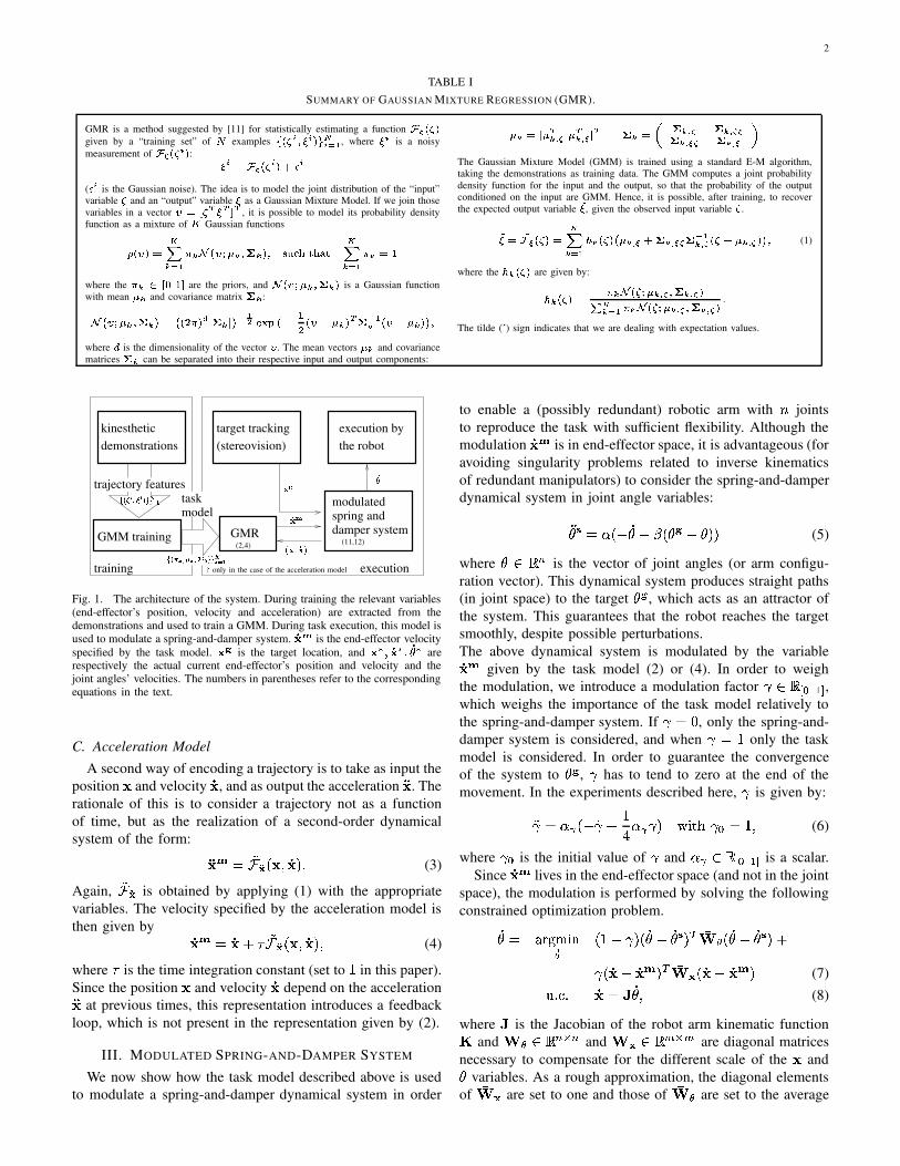
The structure of the system is the same for both modelsand is schematized in Fig. 1. During training, the relevantvariables (end-effector velocity profiles for the velocity model,or end-effector positions, velocities and accelerations for theacceleration model) are extracted from the set of demonstratedtrajectories and used to train a Gaussian Mixture Model(GMM) (see Table I). During reproduction, the trajectory isspecified by a spring-and-damper dynamical system modulatedby the GMM (see section III). The target is tracked by astereo-vision system and is set to be the attractor point ofthe dynamical system. At each time step, the desired velocitycomputed by the model is then fed to a PID controller forexecution. This does not hinder the online adaptation of themovement.

B. Velocity Model

The first way to encode a motion in a GMM, is to considerthe velocity profile of the end-effector as a function of time�������� . Thus, the input variable � is the time and the outputvariable is the velocity, like in the following velocity model:��� ������� ����� (2)

In other words, the movement is modeled as a velocity profile,given by a function of time, which is learned as describedin Table I. Here and henceforth,

�� ����� is the end-effector velocity specified by the task model. ����� is obtainedby applying (1) with the appropriate variables.

2

TABLE ISUMMARY OF GAUSSIAN MIXTURE REGRESSION (GMR).

GMR is a method suggested by [11] for statistically estimating a function �����! #"given by a “training set” of $ examples %��! #&('*)+&,",-/.&!021 , where )/& is a noisymeasurement of �3�4�! #&�" : ) &65 � � �! & "87:9 &( 9,& is the Gaussian noise). The idea is to model the joint distribution of the “input”variable and an “output” variable ) as a Gaussian Mixture Model. If we join thosevariables in a vector ; 5=< 4>2)#>@?A> , it is possible to model its probability densityfunction as a mixture of B Gaussian functionsC �!;�" 5EDFG 021 H GJILK ;NMPO G 'PQ G "R'TS�UWV,XZY*X\[+Y DFG 021 H G 5�]where the H G_^ < `a] ? are the priors, and I �!;NMRO G 'PQ G " is a Gaussian functionwith mean O G and covariance matrix Q G :ILK ;bMPO G 'PQ G " 5 K �!c H "*d�e Q G e f4g 1hjiRk�l K@m ]c �!; m O G " > QZg 1G �!; m O G "�f�'where n is the dimensionality of the vector ; . The mean vectors O G and covariancematrices Q G can be separated into their respective input and output components:

O G 5L< O >G4o p O >G4o � ? > Q G 5rq Q G#o p Q G4o p �Q G#o � p Q G4o �tsThe Gaussian Mixture Model (GMM) is trained using a standard E-M algorithm,taking the demonstrations as training data. The GMM computes a joint probabilitydensity function for the input and the output, so that the probability of the outputconditioned on the input are GMM. Hence, it is possible, after training, to recoverthe expected output variable u) , given the observed input variable .u) 5 u�3�4�! #" 5EDFG 021wv G �! #" K O G4o �37:Q G4o � p QZg 1G#o p �! m O G4o p "�f�' (1)

where the v G �! #" are given by:

v G �! #" 5 H G I �x 4MPO G4o p 'RQ G4o p "y DG 021 H G�I �! �MPO G4o p '(Q G4o p "bzThe tilde (u ) sign indicates that we are dealing with expectation values.

target tracking(stereovision)

execution bythe robotdemonstrations

kinesthetic

GMM training GMR

trajectory featuresmodulatedspring anddamper system

executiontraining

taskmodel

PSfrag replacements {}| ~A� � ��� � ���� �R�{}| ���x� �,�x� ���A� ���� �R� ��+�� �4� ��+� �

������

only in the case of the acceleration model

(2,4) (11,12)

Fig. 1. The architecture of the system. During training the relevant variables(end-effector’s position, velocity and acceleration) are extracted from thedemonstrations and used to train a GMM. During task execution, this model isused to modulate a spring-and-damper system. ���� is the end-effector velocityspecified by the task model. �2� is the target location, and ���W� ��6�W� �� � arerespectively the actual current end-effector’s position and velocity and thejoint angles’ velocities. The numbers in parentheses refer to the correspondingequations in the text.

C. Acceleration Model

A second way of encoding a trajectory is to take as input theposition � and velocity

�� , and as output the acceleration  � . Therationale of this is to consider a trajectory not as a functionof time, but as the realization of a second-order dynamicalsystem of the form:  � ����_¡� �*�£¢ ��j��¤ (3)

Again, �� �� is obtained by applying (1) with the appropriatevariables. The velocity specified by the acceleration model isthen given by ��� � ���¥§¦ �� ¡� �*�£¢ ��j��¢ (4)

where ¦ is the time integration constant (set to ¨ in this paper).Since the position � and velocity

�� depend on the acceleration � at previous times, this representation introduces a feedbackloop, which is not present in the representation given by (2).

III. MODULATED SPRING-AND-DAMPER SYSTEM

We now show how the task model described above is usedto modulate a spring-and-damper dynamical system in order

to enable a (possibly redundant) robotic arm with © jointsto reproduce the task with sufficient flexibility. Although themodulation

�� is in end-effector space, it is advantageous (foravoiding singularity problems related to inverse kinematicsof redundant manipulators) to consider the spring-and-damperdynamical system in joint angle variables: ªN« �­¬®�J¯ �ª ¥r°Z� ªN± ¯ ª ��� (5)

whereª �r��² is the vector of joint angles (or arm configu-

ration vector). This dynamical system produces straight paths(in joint space) to the target

ª ±, which acts as an attractor of

the system. This guarantees that the robot reaches the targetsmoothly, despite possible perturbations.The above dynamical system is modulated by the variable�� given by the task model (2) or (4). In order to weighthe modulation, we introduce a modulation factor ³ �´� < `µ] ? ,which weighs the importance of the task model relatively tothe spring-and-damper system. If ³ �·¶ , only the spring-and-damper system is considered, and when ³ � ¨ only the taskmodel is considered. In order to guarantee the convergenceof the system to

ª ±, ³ has to tend to zero at the end of the

movement. In the experiments described here, ³ is given by:¸³ �T¬j¹º��¯=»³ ¯ ¨¼ ¬½¹ ³ �¿¾aÀAÁ/ ³ ` � ¨ ¢ (6)

where ³ ` is the initial value of ³ and ¬ ¹ �L� < `Ã] ? is a scalar.Since

�� lives in the end-effector space (and not in the jointspace), the modulation is performed by solving the followingconstrained optimization problem.�ª � ÄNÅ/ÆNÇÈÀ!É�Ê � ¨ ¯ ³ ��� �ª ¯ �ª « ��ËÍÌÎ Ê � �ª ¯ �ª « �j¥

³ � ��L¯ ���Ï�JËÐÌÎ � � ��´¯ ���Ï� (7)Ñ�¤ ÒN¤ ��=�ÔÓ �ª ¢ (8)

where Ó is the Jacobian of the robot arm kinematic functionÕand ÌÎ Ê �´�Ö²º×6² and ÌÎ � �Ø���_×6� are diagonal matrices

necessary to compensate for the different scale of the � andªvariables. As a rough approximation, the diagonal elements

of ÌÎ � are set to one and those of ÌÎ Ê are set to the average

3

distance between the robot base and its end-effector.The solution to this minimization problem is given by [12]:�ª � Ù Î Ê ¥ÚÓ�Ë Î � Ó½Û m ] Ù Î Ê �ª « ¥§Ó�Ë Î � ���ÜÛ (9)¾aÂ�Ý\Å/Ý Î Ê � � ¨ ¯ ³ �ÞÌÎ Ê ¢ Î � � ³ ÌÎ � ¤ (10)

To summarize, the task is performed by integrating thefollowing dynamical system: ªN« � ¬ß��¯ �ª ¥§°ß� ªN± ¯ ª �+� (11)�ª � Ù Î Ê ¥§Ó�Ë Î � Ó½Û m ] Ù Î Ê �ª « ¥ÚÓ�Ë Î � ���ÜÛ (12)

whereÎ � and

Î Ê are given by (6) and (10), and�� is

given either by (2) (velocity model) or by (4) (accelerationmodel). Integration is performed using a first-order Newtonapproximation (

�ª « � �ª ¥r¦  ª « ).Since the target location is given in cartesian coordinates,

inverse kinematics must be performed in order to obtain thecorresponding target joint angle configuration which willserve as input of the spring-and-damper dynamical system.In the case of a redundant manipulator (such as the robotarm used in the following experiments) the desired redundantparameters of the target joint angle configuration can beextracted from the demonstrations. This is done by using theGMR technique described in Table I to build a model of thefinal arm configuration as a function of the target location.

Using an attractor system in joint angle space has thepractical advantage of reducing the usual problems relatedto end-effector control, such as joint limit and singularityavoidance. Equation 9, which is a generalized version ofthe Damped Least Squares inverse [13] [14], is a way tosimultaneously control the joint angles and the end-effector,imposing soft constraints on both of them. It is thus differentthan optimizing the joint angles in the null space of thekinematic function.

IV. EXPERIMENTS

A. Setup

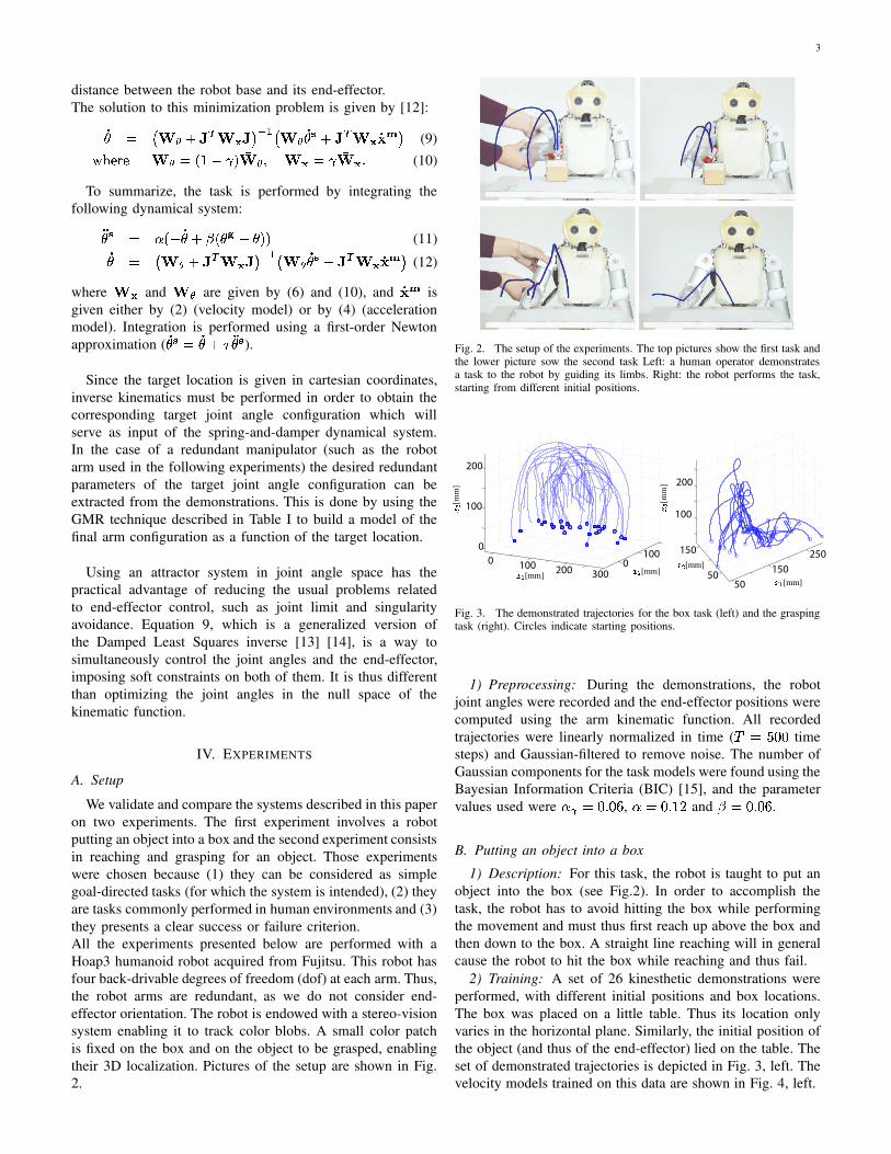
We validate and compare the systems described in this paperon two experiments. The first experiment involves a robotputting an object into a box and the second experiment consistsin reaching and grasping for an object. Those experimentswere chosen because (1) they can be considered as simplegoal-directed tasks (for which the system is intended), (2) theyare tasks commonly performed in human environments and (3)they presents a clear success or failure criterion.All the experiments presented below are performed with aHoap3 humanoid robot acquired from Fujitsu. This robot hasfour back-drivable degrees of freedom (dof) at each arm. Thus,the robot arms are redundant, as we do not consider end-effector orientation. The robot is endowed with a stereo-visionsystem enabling it to track color blobs. A small color patchis fixed on the box and on the object to be grasped, enablingtheir 3D localization. Pictures of the setup are shown in Fig.2.

Fig. 2. The setup of the experiments. The top pictures show the first task andthe lower picture sow the second task Left: a human operator demonstratesa task to the robot by guiding its limbs. Right: the robot performs the task,starting from different initial positions.

0 100 200 3000

1000

100

200

50

150

250

50

150

100

200

PSfrag replacements

à á [mm]à á [mm]

âRã [mm] äRå[mm]

äPæ[mm]ä æ

[mm]

Fig. 3. The demonstrated trajectories for the box task (left) and the graspingtask (right). Circles indicate starting positions.

1) Preprocessing: During the demonstrations, the robotjoint angles were recorded and the end-effector positions werecomputed using the arm kinematic function. All recordedtrajectories were linearly normalized in time ( ç �éè8¶8¶ timesteps) and Gaussian-filtered to remove noise. The number ofGaussian components for the task models were found using theBayesian Information Criteria (BIC) [15], and the parametervalues used were ¬ ¹ �·¶�¤ ¶ëê , ¬ì�·¶�¤ ¨wí and °î�­¶�¤ ¶8ê .B. Putting an object into a box

1) Description: For this task, the robot is taught to put anobject into the box (see Fig.2). In order to accomplish thetask, the robot has to avoid hitting the box while performingthe movement and must thus first reach up above the box andthen down to the box. A straight line reaching will in generalcause the robot to hit the box while reaching and thus fail.

2) Training: A set of 26 kinesthetic demonstrations wereperformed, with different initial positions and box locations.The box was placed on a little table. Thus its location onlyvaries in the horizontal plane. Similarly, the initial position ofthe object (and thus of the end-effector) lied on the table. Theset of demonstrated trajectories is depicted in Fig. 3, left. Thevelocity models trained on this data are shown in Fig. 4, left.

4

0 500−2

−1

0

1

2

time steps

0 500 0 500 0 500 0 500 0 500

“put object in box” task “grasp object” task

PSfrag replacements

ï ð ñï ð ñ ï ð òï ð ò ï ð óï ð ó

Fig. 4. The velocity models for both tasks. The dots represent the trainingdata, the ellipses the Gaussian components and the thick lines the trajectoryobtained by GMR alone. The thick lines show that, for the first task, thehorizontal components ôõ6ö and ôõë÷ are averaged out by the model, but thevertical component ôõ8ø shows a marked upward movement. For the secondtask, all components are almost averaged out.

C. Reach and Grasp

1) Description: In order to accomplish this task, the robothas to reach and correctly place its hand to grasp a chess piece.In other words it has to place its hand so that the chess piecestands between its thumb and its remaining fingers, as shownin Fig. 7, left. This figure illustrates that the approaching theobject can only be done in one of two directions: downwardor forward. This task is more difficult than the previous one,as the movement is more constrained. Moreover, a higherprecision is required on the final position, since the hand isrelatively small.

2) Training: A set of 24 demonstrations were performedstarting from different initial positions located on the horizon-tal plane of the table. The chess piece remained in a fixedlocation. Depending on the initial position, the chess piecewas approached either downward or forward (as illustratedon Fig. 7). The set of demonstrations is represented in Fig.3, right. The resulting velocity model is shown in Fig. 4,right. One can notice that there is no velocity feature thatis common to all demonstrated trajectories. The accelerationmodel is shown in Fig. 5. This model captures well the fact thatthe vertical acceleration component depends on the position inthe horizontal plane.

D. Results

Endowed with the system described above, the robot isable to successfully perform both tasks. For the first task,both the velocity and the acceleration models can produceadequate trajectories (see Fig. 6, left for examples). The systemcan adapt its trajectory online if the box is moved duringmovement execution (see Fig. 6, right). For the second task,examples of resulting trajectories are displayed in Fig. 7, right.In order to evaluate the generalization abilities of the systems,both tasks were executed from various different initial posi-tions arbitrarily chosen on the horizontal plane of the table,and covering the space reachable by the robot. Fig. 8 shows theresults and starting positions for both experiments. For the boxexperiment (left), the velocity model was successful for 22 outof the 24 starting locations (91%). The two unsuccessful trials,

100

200100

0

100

200

300

zm

0 100 200-2

-1

0

1

2

time steps

zd

vertical velocities

trajectories

acceleration model

A

A

A

BB

B

PSfrag replacements ù(ú[mm]

ù ú[mm]

ùRû[mm]

ùRû[mm]

ü ý þ

Fig. 5. In the center, the acceleration model for the second task. The ellipsoidsshow the Gaussian components at twice their standard deviation. Only threeprojections (out of nine) are shown. The vertical acceleration strongly dependson the position in the horizontal plane. On the lower right, two trajectoriesencoded by this model but starting from different positions A and B (indicatedby the crosses) are shown. The corresponding vertical velocity profiles appearon the upper right. They differ significantly, as the model is not homogeneousacross the horizontal plane.

6080

100120

140160

80100

120140

40

60

80

100

120

140

160

2040

6080

100120

80

100

120

40

60

80

100

120

140

160

180

-200

PSfrag replacements ÿ��[mm]

ÿ��[mm]

ÿ� [mm]

ÿ� [mm]

� � [mm

]

� � [mm

]

Fig. 6. Left: end-effector trajectories of the robot putting the object intothe box. The thin line corresponds to the velocity model and the thick linecorresponds to the acceleration model. Right: online trajectory adaptation to atarget displacement using the velocity model. The circles indicate to locationof the box, as tracked by the stereo-vision system. The thick line shows theproduced trajectory and the thin line shows the original trajectory if the boxremained unmoved. Similar results were obtained with the acceleration model.

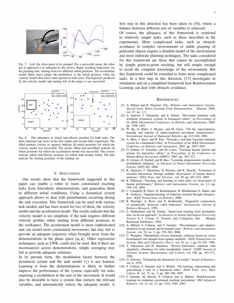
indicated by empty circles, correspond to initial positions closeto the work space boundaries. The acceleration model wassuccessful for all trials (100%).For the chess piece experiment (Fig. 8, right), the velocitymodel was successful for 5 out of 21 (24%) trials whereas theacceleration model was successful for 18 trials (86%). Thisperformance gap is due to the fact that this task does notrequire a fixed velocity modulation. The adequate modulationdepends on the position. This position-dependent modulationcan be captured by the acceleration model, but not by thevelocity model. As illustrated in Fig. 5, the acceleration modelis able to produce different velocity profiles, depending on thestarting position and is thus more versatile than the velocitymodel.

5

60100

140180

80

120

40

80

120

PSfrag replacements ��� [mm]�� [mm]

� [mm

]

Fig. 7. Left: the chess piece to be grasped. For a successful grasp, the robothas to approach it as indicated by the arrows. Right: resulting trajectories forthe grasping task, starting from two different initial positions. The accelerationmodel (thick lines) adapts the modulation to the initial position, while thevelocity model (thin lines) starts upward in both cases. The trajectory producedby the velocity model and starting left of the target is not successful.

50 100 150 200 250 300

0

40

80

120

160

BOX

50 100 150 200 250 300−50

0

50

100

150

chess piece

ROBOTROBOT

success:

vel. model: 91%

acc. model: 100%

success:

vel. model: 24%

acc. model: 86%

PSfrag replacements

�� [mm]�� [mm]

� � [mm

]

� � [mm

]

Fig. 8. The robustness to initial end-effector position for both tasks. Theplots represent top views of the first (right) and second (left) experiment. Thefilled markers (circles or squares) indicate all initial positions for which thevelocity model was successful. The circles (filled and non-filled) indicate allinitial positions for which the acceleration model was successful. The crossesindicate initial end-effector position, for which both models failed. The dotsindicate the starting positions of the training set.

V. DISCUSSION

Our results show that the framework suggested in thispaper can enable a robot to learn constrained reachingtasks from kinesthetic demonstrations, and generalize themto different initial conditions. Using a dynamical systemapproach allows to deal with perturbations occurring duringthe task execution. This framework can be used with varioustask models and has been tested for two of them, the velocitymodel and the acceleration model. The results indicate that thevelocity model is too simplistic if the task requires differentvelocity profiles when starting from different positions inthe workspace. The acceleration model is more sophisticatedand can model more constrained movements, but may fail toprovide an adequate trajectory when brought away from thedemonstrations in the phase space �*�£¢ ��j� . Other regressionstechniques, such as LWR, could also be used. But if there areinconstancies across demonstrations, simple averaging mayfail to provide adequate solutions.In its present form, the modulation factor between thedynamical system and the task model ( ³ ) is not learned.Learning it from the demonstrations is likely to furtherimprove the performance of the system, especially for tasksrequiring a modulation at the end of the movement. It wouldalso be desirable to have a system that extracts the relevantvariables, and automatically selects the adequate model. A

first step in this direction has been taken in [16], where abalance between different sets of variables is achieved.Of course, the adequacy of this framework is restrictedto relatively simple tasks, such as those described in theexperiments. More complicated tasks, such as obstacleavoidance in complex environments or stable grasping ofparticular objects require a detailed model of the environmentand more elaborate planning techniques. The tasks consideredfor this framework are those that cannot be accomplishedby simple point-to-point reaching, but still simple enoughto avoid the complete knowledge of the environment. Butthis framework could be extended to learn more complicatedtasks. In a first step in this direction, [17] investigates insimulation and on a simplified framework how ReinforcementLearning can deal with obstacle avoidance.

REFERENCES

[1] A. Billard and R. Siegwart, Eds., Robotics and Autonomous Systems,Special Issue: Robot Learning From Demonstration. Elsevier, 2004,vol. 47, no. 2,3.

[2] A. Ijspeert, J. Nakanishi, and S. Schaal, “Movement imitation withnonlinear dynamical systems in humanoid robots,” in Proceedings ofthe IEEE International Conference on Robotics and Automation, 2002,pp. 1398–1403.

[3] W. Ilg, G. Bakir, J. Mezger, and M. Giese, “On the representation,learning and transfer of spatio-temporal movement characteristics,”International Journal of Humanoid Robotics, pp. 613–636, 2004.

[4] A. Shon, J. Storz, and R. Rao, “Towards a real-time bayesian imitationsystem for a humanoid robot,” in Proceedings of the IEEE InternationalConference on Robotics and Automation, 2007, pp. 2847–2852.

[5] O. Jenkins, G. Gonzalez, and M. Loper, “Tracking human motion andactions for interactive robots,” in Proceedings of the Conference onHuman-Robot Interaction (HRI07), 2007, pp. 365–372.

[6] D. Grimes, D. Rashid, and R. Rao, “Learning nonparametric models forprobabilistic imitation,” in Advances in Neural Information ProcessingSystems (NIPS 06), 2006.

[7] K. Ogawara, J. Takamatsu, H. Kimura, and K. Ikeuchi, “Extraction ofessential interactions through multiple observations of human demon-strations,” IEEE Trans. Ind. Electron., vol. 50, pp. 667–675, 2003.

[8] R. Dillmann, “Teaching and learning of robot tasks via observation ofhuman performance,” Robotics and Autonomous Systems, no. 2,3, pp.109–116, 2004.

[9] C. Campbell, R. Peters, R. Bodenheimer, W. Bluethmann, E. Huber, andR. Ambrose, “Superpositioning of behaviors learned through teleopera-tion,” IEEE Transactions on Robotics, 2006.

[10] R. Burridge, A. Rizzi, and D. Koditschek, “Sequential compositionof dynamically dexterous robot behaviors,” International Journal ofRobotics Research, 1999.

[11] Z. Ghahramani and M. Jordan, “Supervised learning from incompletedata via an em approach,” in Advances in Neural Information ProcessingSystems 6, J. Cowan, G. Tesauro, and J.Alspector, Eds. MorganKaufmann Publishers, 1994.

[12] A. Billard, S. Calinon, and F. Guenter, “Discriminative and adaptiveimitation in uni-manual and bi-manual tasks,” Robotics and AutonomousSystems, vol. 54, no. 5, pp. 370–384, 2006.

[13] C. Wampler, “Manipulator inverse kinematic solutions based on vectorformulations and damped least-squares methods,” IEEE Transactions onSystems, Man and Cybernetics, Part C, vol. 16, no. 1, pp. 93–101, 1986.

[14] Y. Nakamura and H. Hanafusa, “Inverse kinematics solutions withsingularity robustness for robot manipulator control,” ASME Journal ofDynamic Systems, Measurement, and Control, vol. 108, pp. 163–171,1986.

[15] G. Schwarz, “Estimating the dimension of a model,” Annals of Statistics,vol. 6, 1978.

[16] S. Calinon, F. Guenter, and A. Billard, “On learning, representing andgeneralizing a task in a humanoid robot,” IEEE Trans. Syst., Man,Cybern. B, vol. 37, no. 2, pp. 286–298, 2007.

[17] F. Guenter, M. Hersch, S. Calinon, and A. Billard, “Reinforcementlearning for imitating constrained reaching movements,” RSJ AdvancedRobotics, vol. 21, no. 13, pp. 1521–1544, 2007.