dynamical sampling and its applications by longxiu huang · list of figures figure page 3.1 the...
TRANSCRIPT

Dynamical Sampling and its Applications
By
Longxiu Huang
Dissertation
Submitted to the Faculty of the
Graduate School of Vanderbilt University
in partial fulfillment of the requirements
for the degree of
DOCTOR OF PHILOSOPHY
in
Mathematics
May 10, 2019
Nashville, Tennessee
Approved:
Akram Aldoubi, Ph.D.
Douglas Hardin, Ph.D.
Alexander Powell, Ph.D.
Larry Schumaker, Ph.D.
David Smith, Ph.D.

To the memory of my dear aunt and grandfather,
ii

ACKNOWLEDGMENTS
First and foremost, I would like to express my deepest gratitude to my supervisor Prof. Akram
Aldroubi, for his endless support, guidance, and encouragement. Honestly speaking, I think that I
am the luckiest student in the world. For my research, my supervisor taught me how to ask questions
and how to make baby steps when resolving research projects during my Ph.D. period. I thank him
for carefully reading, commenting and polishing on countless revisions of manuscripts and writing
works for publication. It is a precious privilege for me to have the experience of working with him.
Besides mathematics, I have also learned from him how to deal with tough things in life and how to
keep a positive attitude in life.
I am also profoundly grateful to Prof. Douglas Hardin, Prof. Alexander Powell, Prof. Larry
Schumaker, and Prof. David Smith for serving as my dissertation committee members and their
constructive comments and suggestions on my research work. Additionally, I would like to thank
Prof. Yuesheng Xu and Dr. Weicai Ye for their help and encouragement when I was an under-
graduate and later Ph.D student. In addition, I want to thank all of my collaborators for their great
work and interesting discussions, epscially Prof. Ilya Krishtal, Prof. Keri Kornelson, Prof. Roy
Lederman, Dr. Keaton Hamm, and Dr. Armenak Petrosyan.
Moreover, I want to thank the lovely HAGS (Harmonic Analysis Group) members at Vanderbilt,
especially Prof. David Smith, Dr. Keaton Hamm, Dr. Sui Tang, and Dr. Armenak Petrosyan from
whom I have learned a lot.
Special thanks go to my old friends Tingting Chen and Yachen Wang. Thank them for providing
me companions and encouragement when I was in my hard time. I’m thankful to all my friends
namely at Vanderbilt. They made the time I spent in Nashville enjoyable and meaningful. Special
thanks go to my roommates Bin Gui and Bin Sun, who have helped me a lot in my research and my
daily life.
Most importantly, none of my work would have been accomplished without the love of my fam-
ily. I must thank my parents, elder sister, and younger brother. Their guidance, encouragement, and
support always provided the onward motivation throughout my past journey in life. Meanwhile,
I would like to thank my cousins Tao Wang and Bin Wang, for their patience, guidance, and en-
iii

couragement. Especially, thank Tao Wang for carefully reading, commenting, and polishing on my
writing works.
Finally, I would like to express my deepest gratefulness to my uncle’s family for their kindness
and providing me a positive learning environment. Special thanks to Xuanhao Huang for being a
great cousin.
iv

TABLE OF CONTENTS
Page
ACKNOWLEDGMENTS . . . . . . . . . . . . . . . . . . . . . . . . . . . . . . . . . . . . iii
LIST OF FIGURES . . . . . . . . . . . . . . . . . . . . . . . . . . . . . . . . . . . . . . . vii
Chapter . . . . . . . . . . . . . . . . . . . . . . . . . . . . . . . . . . . . . . . . . . . . . 1
1 INTRODUCTION . . . . . . . . . . . . . . . . . . . . . . . . . . . . . . . . . . . . . 1
1.1 Motivation . . . . . . . . . . . . . . . . . . . . . . . . . . . . . . . . . . . . . . . 1
1.2 Problem Formulation for General Dynamical Sampling . . . . . . . . . . . . . . . 1
1.3 Relation to Other Fields . . . . . . . . . . . . . . . . . . . . . . . . . . . . . . . . 2
1.4 Overview and Organization . . . . . . . . . . . . . . . . . . . . . . . . . . . . . . 3
2 Frames Induced by the Action of Continuous Powers of an Operator . . . . . . . . . . . 4
2.1 Problem Formulation . . . . . . . . . . . . . . . . . . . . . . . . . . . . . . . . . 4
2.2 Recent Results on Dynamical Sampling and Frames . . . . . . . . . . . . . . . . . 4
2.3 Notation and preliminaries . . . . . . . . . . . . . . . . . . . . . . . . . . . . . . 6
2.3.1 Frames . . . . . . . . . . . . . . . . . . . . . . . . . . . . . . . . . . . . 6
2.3.2 Normal operators . . . . . . . . . . . . . . . . . . . . . . . . . . . . . . . 7
2.3.3 Holomorphic Function . . . . . . . . . . . . . . . . . . . . . . . . . . . . 10
2.4 Contributions and Organization . . . . . . . . . . . . . . . . . . . . . . . . . . . . 11
2.5 Completeness . . . . . . . . . . . . . . . . . . . . . . . . . . . . . . . . . . . . . 11
2.5.1 Proofs . . . . . . . . . . . . . . . . . . . . . . . . . . . . . . . . . . . . . 13
2.6 Bessel system . . . . . . . . . . . . . . . . . . . . . . . . . . . . . . . . . . . . . 15
2.6.1 Proofs for Section 2.6 . . . . . . . . . . . . . . . . . . . . . . . . . . . . 16
2.7 Frames generated by the action of bounded normal operators. . . . . . . . . . . . . 23
2.7.1 Proofs of Section 2.7 . . . . . . . . . . . . . . . . . . . . . . . . . . . . . 26
v

3 Dynamical Sampling with Additive Random Noise . . . . . . . . . . . . . . . . . . . . 35
3.1 Problem Formulation . . . . . . . . . . . . . . . . . . . . . . . . . . . . . . . . . 35
3.2 Contribution and Organization. . . . . . . . . . . . . . . . . . . . . . . . . . . . . 36
3.3 Notation and Preliminaries . . . . . . . . . . . . . . . . . . . . . . . . . . . . . . 37
3.3.1 Notation . . . . . . . . . . . . . . . . . . . . . . . . . . . . . . . . . . . 37
3.3.2 A general least squares updating technique for signal recovery . . . . . . . 38
3.3.3 Filter recovery for the special case of convolution operators and uniform
subsampling . . . . . . . . . . . . . . . . . . . . . . . . . . . . . . . . . 40
3.4 Cadzow Denoising Method . . . . . . . . . . . . . . . . . . . . . . . . . . . . . . 43
3.5 Error Analysis . . . . . . . . . . . . . . . . . . . . . . . . . . . . . . . . . . . . . 45
3.5.1 Error analysis for general least squares problems . . . . . . . . . . . . . . 45
3.5.2 Error analysis for dynamical sampling . . . . . . . . . . . . . . . . . . . 47
3.6 Numerical Results . . . . . . . . . . . . . . . . . . . . . . . . . . . . . . . . . . . 48
3.6.1 Error Analysis . . . . . . . . . . . . . . . . . . . . . . . . . . . . . . . . 48
3.6.2 Cadzow Denoising . . . . . . . . . . . . . . . . . . . . . . . . . . . . . . 52
3.6.2.1 Denoising of the sampled data . . . . . . . . . . . . . . . . . . 52
3.6.2.2 Spectrum Reconstruction of the Convolution Operator . . . . . . 53
3.6.3 Real data . . . . . . . . . . . . . . . . . . . . . . . . . . . . . . . . . . . 55
3.7 Concluding remarks . . . . . . . . . . . . . . . . . . . . . . . . . . . . . . . . . . 63
A Appendix for Chapter 3 . . . . . . . . . . . . . . . . . . . . . . . . . . . . . . . . . . . 65
A.1 Appendix for Proposition 3.5.1 . . . . . . . . . . . . . . . . . . . . . . . . . . . 65
BIBLIOGRAPHY . . . . . . . . . . . . . . . . . . . . . . . . . . . . . . . . . . . . . . . 67
vi
LIST OF FIGURES
Figure Page
3.1 The behavior of EpεL22σ2q for randomly generated signal. The signal f is ran-
domly generated with norm 2.2914. Three signals f , 10f , and 100f are used for the
simulations, where x-axis stands for the time levels and y-axis represents the value
of EpεL22σ2q. . . . . . . . . . . . . . . . . . . . . . . . . . . . . . . . . . . . . 48
3.2 The original signals and the reconstructed signals are represented by blue circles and
red stars, respectively. The signals in 3.2c and 3.2d are obtained from the signals in
3.2a and 3.2b, respectively, by multiplying by 10. The norm of the original signal
in 3.2a equals the norm of the original signal in 3.2b, the same is true for the signals
in 3.2c and 3.2d. . . . . . . . . . . . . . . . . . . . . . . . . . . . . . . . . . . . . 49
3.3 The behavior of EpεL22σ2q are shown in (3.3a) and (3.3b) for the sparsely sup-
ported signals without and with applying the threshold method, respectively, where
the samples are corrupted by Gaussian noise with zero mean and standard deviation
2.3714ˆ 10´2. . . . . . . . . . . . . . . . . . . . . . . . . . . . . . . . . . . . . 50
3.4 A comparison of the reconstruction results before and after applying the threshold
method. (3.4a) and (3.4b) show the reconstruction results before and after applying
the threshold method, respectively. In (3.4a) and (3.4b), the original signals have
the same sparse support t8, 9, 10u. The samples are corrupted by the independent
Gaussian noise with mean 0 and standard deviation 2.3714ˆ 10´2. . . . . . . . . 51
3.5 The relative errors using Cadzow denoising method. The vertical axis represents
log10 of averaged (3.18) when the threshold rank in the Cadzow denoising Algo-
rithm 3 is greater than or equal to 3. When the threshold rank is 0 (3.19) is used
instead of (3.18). . . . . . . . . . . . . . . . . . . . . . . . . . . . . . . . . . . . 53
vii

3.6 The relation between the relative errors and the noise standard deviations using
the Cadzow denoising method with different threshold ranks. The curves labeled
“rank “ r”, r “ 3, 7 . . . reflect the relationship between log10 of the averaged
relative errors and log10 of the noise standard deviations, where the relative errors
are represented in (3.18) for rank ě 3 and in (3.19) for rank “ 0. . . . . . . . . . 54
3.7 A comparison of the spectrum reconstruction with and without the Cadzow denois-
ing technique for σ “ 10´5. . . . . . . . . . . . . . . . . . . . . . . . . . . . . . 56
3.8 A comparison of the spectrum reconstruction with and without the Cadzow denois-
ing technique for σ “ 10´4. . . . . . . . . . . . . . . . . . . . . . . . . . . . . . 57
3.9 A comparison of the spectrum reconstruction with and without the Cadzow denois-
ing technique for σ “ 10´3. . . . . . . . . . . . . . . . . . . . . . . . . . . . . . 58
3.10 A comparison of the recovered signal and the original signal by using the estimated
recovered convolution operator. . . . . . . . . . . . . . . . . . . . . . . . . . . . 59
3.11 Set-up. . . . . . . . . . . . . . . . . . . . . . . . . . . . . . . . . . . . . . . . . 60
3.12 Simulation results for the data set with one hotspot. Here, (3.12a) plots the evolved
signals, (3.12b) shows the recovered spectrum by using the data from partial lo-
cations, and (3.12c) sketches the recovered signal by using the recovered operator
from partial locations and the sampled original signal. The partial locations for re-
covering the operator are Ω “ t1, 4, 7, 10, 13u. To recover the original signals, we
use the data from locations Ωe “ t1, 3, 4, 7, 10, 13, 15u. . . . . . . . . . . . . . . 61
viii
3.13 Simulation results for the data set with two hotspots. Here, (3.13a) plots the evolved
signals, (3.13b) shows the recovered spectrum by using the data from partial loca-
tions, and (3.13c) sketches the recovered signal by using the recovered operator
from partial locations and the sampled original signal. The partial locations for re-
covering the operator are Ω “ t2, 5, 8, 11, 14u. To recover the original signals, we
use the data from locations Ωe “ t2, 3, 5, 8, 10, 11, 14u. . . . . . . . . . . . . . . 62
3.14 Simulation results for the data set with one hotspot. Here, (3.14a) shows the re-
covered spectrum by using the data from partial locations, while (3.14b) plots the
recovered signal by using the recovered operator from partial locations, where the
partial locations for recovering the operator are Ω “ t2, 5, 8, 11, 14u. To recover
the original signals, we use the samples from locations Ωe “ t2, 3, 5, 8, 10, 11, 14u. 63
ix

CHAPTER 1
INTRODUCTION
1.1 Motivation
A typical problem in sampling theory is to reconstruct a function (signal) f in a separable Hilbert
space from its samples, for which a natural approach would be to sample the function f at as many
accessible positions as possible. In general, one expects that, with some a priori information, f can
be reconstructed from those samples. This idea motivates the classical sampling theory. Related
results can be consulted in, e.g., [3, 4, 8, 16, 20, 53, 54]. However, there are various restrictions in
real-world applications. For example, sensors may not be permitted to be installed at some required
locations. Moreover, the spatial sampling density can be very limited, because sensors are often
expensive and it is costly to achieve a high sampling density.
On the other hand, in many instances, the function f comes from an evolving system which is
driven by a (partially) known operator, and the feature of the function can be exploited to compen-
sate for the insufficiency in sampling locations. An intuitive example is provided by diffusion and
modeled by the heat equation [43] which exemplifies a spatio-temporal trade-off. Aldroubi and his
collaborators have developed a novel mathematical framework, called dynamical sampling, to study
the spatio-temporal trade-off problem [5, 6, 12]. Dynamical sampling has potential applications in
signal processing, medical imaging, wireless sensor networks, and to name a few.
1.2 Problem Formulation for General Dynamical Sampling
The general formulation can be stated as follows. Let f be a vector in a Hilbert space pH, x¨, ¨yq
and A be a bounded linear operator on H. The initial signal f evolves, and at time t becomes
ft “ Atf.
1

Given a countable (finite or countably infinite) set of vectors G Ă H, the samples (measurements)
over a time set T are of the form
M “
xAtf, gy : g P G, t P T(
.
The general dynamical sampling problem can be described as
Problem 1. What are the conditions on the operator A, the sampling set G, and the time set T Ă
r0,8q such that any function f P H can be recovered or stably recovered from M?
Remark 1.2.1. In general, the measurements
xAtf, gy : g P G(
at every single time point t P T
are insufficient to recover Atf . In other words, Atf is undersampled.
By the recovery of f we mean that there exists an operator R from G ˆ T to H such that
RpxAtf, gyq “ f for all f P H. If R is bounded, then we say that the recovery of f is stable. Using
the relation between A and its adjoint operator A˚, Problem 1 is equivalent to
Problem 2. What are the conditions on the operator A, G, and the time set T Ă r0,8q that ensure
that the system tA˚tg : g P G, t P T u is complete or a (continuous) frame for H?
Because of this equivalence, we can investigate Problem 2 instead of Problem 1. For the nota-
tional simplicity, we drop the * and study the system of the form tAtg : g P G, t P T u in Problem
2.
1.3 Relation to Other Fields
Dynamical sampling, as a new sampling theory, has relations with other areas of mathematics.
For instance, it has similarities with wavelet theory [18, 29, 36, 38]. In wavelet theory, a high-pass
operator H and a low-pass operator L are applied to the function f . The goal is to design operators
H and L so that the reconstruction of f from the combined samples of Hf and Lf is possible.
Similarly, in dynamical sampling the main purpose is to reproduce f via the samples M collected
from different time points. However, in dynamical sampling there is only one operator A, which
acts on the function f iteratively. There is no specific structural restrictions on A.
2

Dynamical sampling has close relation with inverse problems (see [47] and the references
therein). An inverse problem is the process of finding the factors that result in a set of observa-
tions. The main goal of dynamical sampling is thus the inverse problem of finding the factor f from
the knowledge of the driving operatorA and the set M “ txAtf, gy : t P T, g P Gu of observations.
If the full information of A is given, then the inverse problem is linear. Otherwise, the problem
is non-linear and in this case we also want to recover the operator A. In other words, we ask the
following question.
Question 1. What are the conditions on A, T , and G such that A and f can be recovered from the
observed data M?
In addition, methods to solve dynamical sampling problems have close relation with spectral
theory, operator algebras, numerical linear algebra, frame theory, and complex analysis.
1.4 Overview and Organization
In the existing studies of dynamical sampling, only the case for discrete time sets T has been
considered. However, time is continuous in the physical world, and thus it is natural to consider the
dynamical sampling problem for continuous time intervals T . This work is presented in Chapter 2.
In this work, we consider systems of the form tAtg : g P G, t P r0, Lsu Ă H, whereA P BpHq. The
goal is to study the frame property of such systems. To this end, we derive some other properties
in the intermediate steps. In particular, we study the completeness and Besselness of these systems.
These results are a joint work with Akram Aldroubi and Armenak Petrosyan and it is documented in
the preprint entitled “Frames induced by the action of continuous powers of an operator”, see [11].
In addition, noises are ubiquitous in real world and sampling applications which necessitates
an investigation of the impacts of noise on dynamic sampling. The related results are reported in
Chapter 3. The work is joint with Akram Aldroubi, Ilya Krishtal, Akos Ledeczi, Roy R. Lederman,
and Peter Volgyesi and appears in [9, 10].
3

CHAPTER 2
Frames Induced by the Action of Continuous Powers of an Operator
2.1 Problem Formulation
In this chapter, we consider dynamical sampling with the time set belonging to a bounded in-
terval. Specifically, we investigate systems of the form tAtg : g P G, t P r0, Lsu, where A is a
bounded linear normal operator in a separable Hilberst space H, G Ă H is a countable set, and L is
a positive real number. The main goal is to investigate the following problems.
Problem 3. What are the conditions onA, G, andL that ensure that system tAtg : g P G, t P r0, Lsu
is complete, Bessel, or a continuous frame in H?
The discretization of continuous frames [31, 32] is a central question. For systems of the form
tAtg : g P G, t P r0, Lsu, we ask
Problem 4. Suppose tAtg : g P G, t P r0, Lsu is a continuous frame. Is there a partition 0 “ t1 ă
t2 ă . . . ă tn ă L of r0, Ls such that the system tAtig : g P G, 1 ď i ď n and i P Nu is a discrete
frame (see inequality (2.1))?
2.2 Recent Results on Dynamical Sampling and Frames
Existing studies on various aspect of the dynamical sampling problem and related frame theory
grew out of the work in [1, 5, 6, 7, 42, 49], see, for example, [2, 21, 22, 24, 40, 45, 46, 48, 56, 57]
and the references therein. However, except for a few, they all focus on uniform discrete-time sets
T Ă t0, 1, 2, . . .u, e.g., T “ t1, . . . , Nu or T “ N (see e.g., [36]).
Even though the general dynamical sampling problem for discrete-time sets in finite dimen-
sions (hence problems of systems and frames induced by iterations tAng : g P G, n P T u) have
been mostly resolved in [6], many problems and conjectures remain open for the infinite dimen-
sional case. This state of affairs is not surprising because some of these problems take root in the
deep theory of functional analysis and operator theory such as the Kadison Singer Theorem [44],
4

some open generalizations of the Muntz-Szasz Theorem [51], and the famous invariant subspace
conjecture.
When T “ N and A P BpHq, it is not difficult to show that
Theorem 2.2.1 ([13]). If, for an operator A P BpHq, there exists a countable set of vectors G in H
such that tAngugPG, ně0 is a frame in H, then for every f P H, pA˚qnf Ñ 0 as nÑ8.
Thus, in particular it is not possible to construct frames using non-negative iterations when A is
a unitary operator. For example, the right-shift operator S on H “ `2pNq generates an orthonormal
basis for `2pNq by iterations over G “ tp1, 0, . . . , qu. Clearly, pS˚qnf Ñ 0 as nÑ8 for this case.
However, if we change the space to H “ `2pZq, the right-shift operator S becomes unitary, and
there exists no subset G of `2pZq such that tSngugPG, ně0 is a frame for `2pZq.
On the other hand, for normal operators, it is possible to find frames of the form tAngugPG, ně0;
however, no such a frame can be a basis [5].
Frames for H can be generated by the iterative action on a single vector g, i.e., there exist normal
operators and associated cyclic vectors such that tAngu ně0 is a frame for H [6]. Specifically,
Theorem 2.2.2 ([5]). LetA be a bounded normal operator on an infinite dimensional Hilbert space
H. Then, tAnguně0 is a frame for H if and only if the following five conditions are satisfied:
(i) A “ř
j λjPj , where Pj are rank one orthogonal projections; (ii) |λk| ă 1 for all k; (iii)
|λk| Ñ 1; (iv) tλku satisfies Carleson’s condition infnś
k‰n|λn´λk|
|1´λnλk|ě δ, for some δ ą 0; and
(v) 0 ă c ďPjg?1´|λk|2
ď C ă 8, for some constants c, C.
It turns out that if A is normal in an infinite dimensional Hilbert space H, and tAngugPG, ně0
is a frame for some G Ă H with |G| ă 8, then A is necessarily of the form described in Theorem
2.2.2:
Theorem 2.2.3 ([13]). Let A be a bounded normal operator in an infinite dimensional Hilbert
space H. If the system of vectors tAngugPG, ně0 is a frame for some G Ă H with
|G| ă 8, then A “ř
j λjPj where Pj are projections such that rank pPjq ď |G|
pi.e., the global multiplicity of A is less than or equal to |G|q . In addition, (ii) and (iii) of Theorem
2.2.2 are satisfied.
5

The necessary and sufficient conditions generalizing Theorem 2.2.2 for the case 1 ă |G| ă 8
have been derived in [21].
Viewing Theorem 2.2.2 from a different perspective, Christensen and Hasannasab ask whether a
frame thnunPI has a representation of the form hn “ Anh0 for some operator A when I “ NYt0u
or I “ Z. This question is partially answered in [25] and gives rise to many new open problems and
conjectures [24].
The set of self-adjoint operators is an important class of normal operators because it is often
encountered in applications. For this class, one can rule out certain types of normalized frames.
Theorem 2.2.4 ([6]). If A is a self-adjoint operator on H, then the system!
Ang‖Ang‖
)
gPG, ně0is not
a frame for H.
However, for normal operators, the following conjecture remains open:
Conjecture 2.2.5. The statement of Theorem 2.2.4 holds for normal operators.
Conjecture 2.2.5 does not hold if the operator is not normal. For example, the shift-operator S
on `2pNq defined by Spx1, x2, . . . q “ p0, x1, x2, . . . q, is not normal, and tSne1u is an orthonormal
basis for `2pNq, where e1 “ p1, 0, . . . q.
2.3 Notation and preliminaries
2.3.1 Frames
In a foundational paper, Duffin and Schaeffer introduced the theory of frames in the context of
non-harmonic Fourier series [30]. Specifically, a frame tφnunPZ in a separable Hilbert space H is a
sequence of vectors satisfying
c f2 ďÿ
nPZ|xf, φny|
2ď Cf2, for all f P H, (2.1)
for some positive constants c, C ą 0. Later, the notion in (2.1) is generalized to continuous frames
[14, 15, 31, 33], where the definition is stated below:
Definition 2.3.1. Let H be a complex Hilbert space and let pΩ, µq be a measure space with positive
measure µ. A mapping F : Ω Ñ H is called a frame with respect to pΩ, µq, if
6

1. F is weakly-measurable, i.e., ω Ñ xf, F pωqy is a measurable function on Ω for all f P H;
2. there exist constants c and C ą 0 such that
cf2 ď
ż
Ω|xf, F pωqy|2dµpωq ď Cf2, for all f P H. (2.2)
Here the constants c and C are called continuous frame (lower and upper) bounds. In addition, F
is called a tight continuous frame if c “ C. The mapping F is called Bessel if the second inequality
in (2.2) holds. In this case, C is called a Bessel constant.
The frame operator S “ SF on H associated with F is defined in the weak sense by
SF f “
ż
Ωxf, F pωqyF pωqdµpωq.
According to (2.2), SF is well defined, invertible with bounded inverse (see [31]). Thus every f P H
has the representations
f “ S´1F SF f “
ż
Ωxf, F pωqyS´1
F F pωqdµpωq,
f “ SFS´1F f “
ż
Ωxf, S´1
F F pωqyF pωqdµpωq.
If µ is the counting measure and Ω “ N, then one gets back the Duffin-Schaffer frame in (2.1).
In the sequel, Ω “ G ˆ r0, Ls, and µ is the product of the counting measure on G and the
Lebesgue measure on r0, Ls. In this case, F is called a semi-continuous frame and (2.2) becomes
cf2 ďÿ
gPG
Lż
0
|xf,Atgy|2dt ď Cf2, for all f P H. (2.3)
2.3.2 Normal operators
Let BpHq denote the space of bounded linear operators on a complex separable Hilbert space
H. In the sequel, all the operators are assumed to be normal. Normal operators have the following
invertibility property (see [52, Theorem 12.12]).
7

Theorem 2.3.2. If A P BpHq, then A is invertible pi.e., A has bounded inverseq if and only if there
exists c ą 0 such that Af ě cf for all f P H.
For completeness, the spectral theorem with multiplicity is stated below, and the following
notation is used in its statement.
For a non-negative regular Borel measure µ on C, Nµ will denote the multiplication operator
acting on L2pµq, i.e., for a µ-measurable function f : CÑ C such thatş
C |fpzq|2dµpzq ă 8,
Nµfpzq “ zfpzq.
We will use the notation rµs “ rνs to denote two mutually absolutely continuous measures µ
and ν.
The operator N pkqµ will denote the direct sum of k copies of Nµ, i.e.,
pNµqpkq “ ‘ki“1Nµ.
Similarly, the space pL2pµqqpkq will denote the direct sum of k copies of L2pµq.
Theorem 2.3.3 (Spectral theorem with multiplicity). For any normal operator A on H there are
mutually singular non-negative Borel measures µj , 1 ď j ď 8, such that A is equivalent to the
operator
N p8qµ8 ‘Nµ1 ‘Np2qµ2 ‘ . . . ,
i.e., there exists a unitary transformation
U : HÑ pL2pµ8qqp8q ‘ L2pµ1q ‘ pL
2pµ2qqp2q ‘ . . .
such that
UAU´1 “ N p8qµ8 ‘Nµ1 ‘Np2qµ2 ‘ . . . . (2.4)
Moreover, if A is another normal operator with corresponding measures ν8, ν1, ν2, . . ., then A is
unitary equivalent to A if and only if rνjs “ rµjs for j “ 1, . . . ,8.
A proof of the theorem can be found in [28, Ch. IX, Theorem 10.16] and [27, Theorem 9.14].
8

Since the measures µj are mutually singular, there are mutually disjoint Borel sets tEju8j“1 Y
tE8u such that µj is supported on Ej for every 1 ď j ď 8. The scalar-valued spectral measure µ
associated with the normal operator A is defined as
µ “ÿ
1ďjď8
µj . (2.5)
The Borel function mA : CÑ N˚ Y t0u given by
mApzq “ 8 ¨ χE8pzq `8ÿ
j“1
jχEj pzq (2.6)
is called the multiplicity function of the operator A, where N is the set of natural numbers start-
ing with 1, N˚ “ N Y t8u, χEpzq is the characteristic function on set E defined by χEpzq “$
’
’
&
’
’
%
1, z P E
0, otherwiseand8 ¨ 0 “ 0.
From Theorem 2.3.3, every normal operator is uniquely determined, up to a unitary equivalence,
by the pair prµs,mAq.
For j P N, let Ωj be the set t1, ..., ju and let Ω8 be the set N. Then `2pΩjq – Cj , for j P N,
and `2pΩ8q “ `2pNq. For j “ 0, we use `2pΩ0q to represent the trivial space t0u.
Let W be the Hilbert space
W “ pL2pµ8qqp8q ‘ L2pµ1q ‘ pL
2pµ2qqp2q ‘ ¨ ¨ ¨
associated with the operator A and let U : HÑW be the unitary operator given by Theorem 2.3.3.
If g P H, we denote by rg the image of g under U . Since rg PW , one has rg “ prgjqjPN˚ , where rgj is
the restriction of rg to pL2pµjqqpjq. Thus, for any j P N˚, rgj is a function from C to `2pΩjq and
ÿ
jPN˚
ż
Crgjpzq
2`2pΩjq
dµjpzq “ g2 ă 8.
Let Pj be the projection defined for every rg PW by Pjrg “ rf , where rfj “ rgj and rfk “ 0 for k ‰ j.
Let E be the spectral measure for the normal operator A. Then, for every µ-measurable set
9

G Ă C and vectors f, g in H, one has the following formula
xEpGqf, gyH “
ż
G
«
ÿ
1ďjď8
χEj pzqxrfjpzq, rgjpzqy`2pΩjq
ff
dµpzq,
which relates the spectral measure of A to the scalar-valued spectral measure of A.
Definition 2.3.4. Given a normal operator A, At is defined as follows:
At : HÑ H
by
xAtf1, f2y “
ż
zPσpAqztxf1pzq, f2pzqydµpzq, for all f1, f2 P H,
where zt “ expptplnp|z|q ` i argpzqqq and argpzq P r´π, πq.
Using the fact that exppi argpzq ` i argpzqq “ 1, it follows that pA˚qt “ pAtq˚ for t P R.
Section 2.5 will exploit the reductive operators which were introduced by P.Halmos and
J.Wermer [37, 55]. For clarity, the definition is given as follows.
Definition 2.3.5. A closed subspace V Ă H is called reducing for the operator A if both V and its
orthogonal complement V K are invariant subspaces of A.
Definition 2.3.6. An operator A is called reductive if every invariant subspace of A is reducing.
2.3.3 Holomorphic Function
The techniques of complex analysis, e.g., the properties of holomorphic functions (see [26, 51]
and the references therein), are used extensively in the present work, including Montel’s Theorem
as stated below.
Definition 2.3.7 (Normal family). A family F of holomorphic functions in a region X of the com-
plex plane with values in C is called normal if every sequence in F contains a subsequence which
converges uniformly to a holomorphic function on compact subsets of X.
Theorem 2.3.8 (Montel’s Theorem). A uniformly bounded family of holomorphic functions defined
on an open subset of the complex numbers is normal.
10
2.4 Contributions and Organization
The present work concentrates on systems of the form tAtg : g P G, t P r0, Lsu Ă H, where
A P BpHq. The goal is to study the frame property of such systems. To this end, we need to
derive some other properties in the intermediate steps. In particular, we study the completeness and
Besselness of these systems.
For the completeness of tAtg : g P G, t P r0, Lsu, necessary and sufficient conditions are de-
rived in Section 2.5. In light of the results in [5], the form of the necessary and sufficient conditions
are not surprising. However, the proofs and reductions to the known cases are appealing due to the
use of certain techniques of complex analysis, and they are useful for the analysis of frames in the
subsequent sections.
The Bessel property of the system tAtg : g P G, t P r0, Lsu is investigated in Section 2.6.
Specifically, if H is a finite dimensional space (e.g., Cd) and A is a normal operator in H, then the
system tAtgugPG,tPr0,Ls being Bessel is equivalent to the Besselness of G in the space RangepAq.
On the other hand, if H is an infinite dimensional separable Hilbert space and A is a bounded
invertible normal operator, then the only condition ensuring that tAtgugPG,tPr0,Ls is Bessel is that G
itself is a Bessel system in H. In addition, an example is described to explain that the non-singularity
of A is necessary for the equivalence between the Besselness of tAtgugPG,tPr0,Ls and that of G.
Section 5 is devoted to the relations between a semi-continuous frame tAtgugPG,tPr0,Ls generated
by the action of an operator A P BpHq and the discrete systems generated by its time discretization.
Specifically, we show that under some mild conditions, tAtgugPG,tPr0,Ls is a semi-continuous frame
if and only if there exists T “ tti : i “ Iu Ă r0, Lq with |I| ă 8 such that tAtgugPG,tPT is a
frame system in H. Additionally, Theorem 2.7.5 shows that under proper conditions, the property
that tAtgugPG,tPr0,Ls is a semi-continuous frame is independent of L.
2.5 Completeness
In this section, we characterize the completeness of the system tAtgugPG,tPr0,Ls, where A is a
(reductive) normal operator on a separable Hilbert space H, G is a set of vectors in H, and L is a
finite positive number.
11

Theorem 2.5.1. Let A P BpHq be a normal operator, and let G be a countable set of vectors in H
such that tAtgugPG,tPr0,Ls is complete in H. Let µ8, µ1, µ2, . . . be the measures in the representation
(2.4) of the operator A. Then for every 1 ď j ď 8 and µj-a.e. z, the system of vectors tgjpzqugPG
is complete in `2pΩjq.
If A is also reductive, then tAtgugPG,tPr0,Ls being complete in H is equivalent to tgjpzqugPG
being complete in `2pΩjq µj-a.e. z for every 1 ď j ď 8.
Particularly, if the evolution operator belongs to the following class A of bounded self-adjoint
operators:
A “ tA P Bp`2pNqq : A “ A˚,
and there exists a basis of `2pNq of eigenvectors of Au, (2.7)
then, for A P A, there exists a unitary operator U such that A “ U˚DU with D “ř
j λjPj , where
λj are the spectrum of A and Pj is the orthogonal projection to the eigenspace Ej of D associated
with the eigenvalue λj . Since the operators in A are also normal and reductive, the following
corollary holds.
Corollary 2.5.2. Let A P A with A “ U˚DU , and let G be a countable set of vectors in `2pNq.
Then, tAtgugPG,tPr0,Ls is complete in `2pNq if and only if tPjpUgqugPG is complete in Ej .
The proof of Theorem 2.5.1 below, also shows that, for normal reductive operators, complete-
ness in H is equivalent to completeness of the system tN tµj gjugPG,tPr0,Ls in pL2pµjqq
pjq for every
1 ď j ď 8. In other words, the completeness of tAtgugPG,tPr0,Ls is equivalent to the completeness
of its projections onto the mutually orthogonal subspaces U˚PjUH of H. The following Theorem
2.5.3 summarizes the discussion above.
Theorem 2.5.3. Let A P BpHq be a normal reductive operator on the Hilbert space H, and let G
be a countable system of vectors in H. Then, tAtgugPG,tPr0,Ls is complete in H if only if the system
tN tµj gjugPG,tPr0,Ls is complete in pL2pµjqq
pjq for every j, 1 ď j ď 8.
12

2.5.1 Proofs
We begin this section by stating and proving a lemma used to prove Theorem 2.5.1 as well as
other results in later sections.
LetA be a normal operator, L be a positive number, f P H, f “ Uf “ pfjq, and g “ Ug “ pgjq
(as in the notation section). Define F ptq by
F ptq “ xAtg, fy “
ż
Cztxgpzq, fpzqydµpzq.
Then, the following lemma holds.
Lemma 2.5.4. F ptq is an analytic function of t in the domain Ω “ tt : <ptq ą L2u, where <ptq
stands for the real part of t.
Proof. First, we aim to prove that F ptq is a continuous function in Ω. Consider t0 P Ω. For
|z| ďM, where M “ A, and for t P Ω with |t´ t0| ă L4, one has
|ztxgpzq, fpzqy| “ |et lnpzq||xgpzq, fpzqy|
ď ep| lnpMq|`πq|t||xgpzq, fpzqy|
ď ep| lnpMq|`πqp|t0|`L4q|xgpzq, fpzqy|.
Since the right hand side of the last inequality is an L2pµq function, we can use the dominated
convergence theorem for <ptq ą L2 ą 0, and get that for t0 P Ω,
limtÑt0
F ptq “ limtÑt0
ż
Cztxgpzq, fpzqydµpzq “
ż
ClimtÑt0
ztxgpzq, fpzqydµpzq “ F pt0q.
Therefore, F ptq is a continuous function in Ω.
Next we show that for every closed piecewise C1 curve γ in Ω,
¿
γ
F ptqdt “ 0.
13

For fixed γ, there exists finite M1 ą 0 such that L2 ă |t| ăM1. Therefore, for |z| ďM ,
|ztxgpzq, fpzqy| ď eM |xgpzq, fpzqy|,
with M “M1p| lnM | ` πq. Then
¿
γ
ż
C|zt||xgpzq, fpzqy|dµpzqdt ď eMf2g2 ¨m1pγq ă 8,
where m1pγq stands for the length of γ.
By Fubini’s theorem,
¿
γ
ż
Cztxgpzq, fpzqydµpzqdt “
ż
C
¿
γ
ztxgpzq, fpzqydtdµpzq
“
ż
Cxgpzq, fpzqy
¿
γ
ztdtdµpzq “ 0.
where the last equality follows from the fact that for z P C, hzptq “ zt is an analytic function of t
in Ω and henceű
γ ztdt “ 0. Then, by Morera’s Theorem [51, pp 208], F ptq is analytic on Ω.
Proof of Theorem 2.5.1. Since tAtgugPG,tPr0,Ls is complete in H,
UtAtg : g P G, t P r0, Lsu “ tpN tµj gjqjPN˚ : g P G, t P r0, Lsu
is complete in W “ UH. Hence, for every 1 ď j ď 8, the system rSj “ tN tµj gjugPG,tPr0,Ls is
complete in pL2pµjqqpjq.
To finish the proof of the first statement of Theorem 2.5.1 we use the following lemma, which
is an adaptation of [39, Lemma 1] ([5, Lemma 3.5]).
Lemma 2.5.5. Let S be a complete countable set of vectors in pL2pµjqqpjq, then for µj-almost
every z, thpzq : h P Su is complete in `2pΩjq.
Since H is separable, there exists a countable set T “ ttiu8i“1 Ă r0, Ls with t1 “ 0 such
that spantAtgugPG,tPT “ spantAtgugPG,tPr0,Ls. Hence, the fact that rSj “ tN tµj gjugPG,tPr0,Ls is
complete in pL2pµjqqpjq (together with Lemma 2.5.5) implies that tztgjpzqugPG,tPT is complete in
14

`2pΩjq for each j P N˚. Let f P H and F ptq “ xAtg, fy “ 0 for all g P G, t P r0, Ls. Since
F ptq “ 0 for all t P r0, Ls, and F is analytic for t P Ω “ tt : <ptq ą L2u, it follows that
F ptq “ 0, for all t P Ω (see [51, Theorem 10.18]). Thus, F pnq “ 0 for all n P N, i.e., for all n P N,
ż
Cznxgpzq, fpzqydµpzq “
ż
Czn
«
ÿ
1ďjď8
χEj pzqxgjpzq, fjpzqy`2pΩjq
ff
dµpzq “ 0. (2.8)
To finish the proof, we need the following proposition from [55].
Proposition 2.5.6. Let A be a normal operator on the Hilbert space H and let µj be the measures
in the representation (2.4) of A. Let µ be as in (2.5). Then, A is reductive if and only if, for any two
vectors f, g P H,ż
Czn
«
ÿ
1ďjď8
χEj pzqxgjpzq, fjpzqy`2pΩjq
ff
dµpzq “ 0
for every n ě 0 implies µj-a.e. xgjpzq, fjpzqy`2pΩjq“ 0 for every j P N˚.
Since A is reductive, it follows from Proposition 2.5.6 that xgjpzq, fjpzqy`2pΩjq“ 0 for
every j P N˚. Finally, since tgjpzqugPG is complete in `2pΩjq for µj-a.e. z, we get that
fjpzq “ 0, µj-a.e. z for every j P N˚. Thus, f “ 0 µ-a.e. z, and hence f “ 0. Therefore,
tAtgugPG,tPr0,Ls is complete in H.
2.6 Bessel system
The goal of this section is to study the conditions for which the system tAtgugPG,tPr0,Ls is Bessel
in H. There are two main theorems that correspond to the finite dimensional case and the infinite
dimensional case, respectively. The proofs of the results are relegated to the last subsection. We
begin with the following proposition which is valid for both finite and infinite dimensional spaces.
Proposition 2.6.1. Let A P BpHq be normal, G Ă H be a countable set of vectors, and let L be a
positive finite number. If G is a Bessel system in H, then tAtgugPG,tPr0,Ls is a Bessel system in H.
The fact that G is a Bessel system in H implies that tAtgugPG,tPr0,Ls is Bessel in H is not too
surprising. However, the converse implication is not obvious. The next result characterizes the finite
dimensional case.
15

Theorem 2.6.2 (Besselness in finite dimensional space). Let A be a normal operator on Cd and
L be a positive finite number. Let M “ RangepA˚q and PMG “ tPMgugPG , where PM is the
orthogonal projection on M . Then, tAtgugPG,tPr0,Ls is a Bessel system in Cd if and only if PMG is
a Bessel system in M .
Under the appropriate restrictions on the spectrum σpAq of A, one can obtain a result similar
to Theorem 2.6.2 for the infinite dimensional case. However, if 0 R σpAq, the main result for the
infinite dimensional Hilbert space is stated in the following theorem.
Theorem 2.6.3 (Besselness in infinite dimensions). Let A P BpHq be an invertible normal op-
erator, and let G be a countable system of vectors in H. Then, for any finite positive number L,
tAtgugPG,tPr0,Ls is a Bessel system in H if and only if G is a Bessel system in H.
The condition thatA is invertible is necessary in Theorem 2.6.3 as can be shown by the following
example.
Example 1. Let G “ tnenu8n“1 with tenu8n“1 being the standard basis of `2pNq, f P `2pNq with
fpnq “ 1n, and let D be the diagonal infinite matrix with diagonal entries Dn,n “ e´n2. The
operator D is injective but not an invertible operator on `2pNq.
Note thatÿ
gPG|xf, gy|2 “ 8.
Hence, G is not a Bessel system in `2pNq. On the other hand,
ÿ
gPG
ż 1
0|xf,Dtgy|dt “
8ÿ
n“1
1´ e´2n2
2|fn|
2 ď f22. (2.9)
Thus tDtgugPG,tPr0,1s is Bessel in `2pNq.
2.6.1 Proofs for Section 2.6
Proof of Proposition 2.6.1. For all f P H,
ÿ
gPG
Lż
0
|xf,Atgy|2dt “ÿ
gPG
Lż
0
|xA˚tf, gy|2dt
16

“
Lż
0
ÿ
gPG|xA˚tf, gy|2dt ď
Lż
0
CGA˚tf2dt
ď
Lż
0
CGA2tf2dt “
$
’
’
&
’
’
%
CGA2L´1ln A2
f2, A ‰ 1
CGLf2, A “ 1,
where CG is a Bessel constant of the Bessel system G. Therefore, tAtgugPG,tPr0,Ls is Bessel in
H.
In order to prove Theorem 2.6.2, we need the following lemma:
Lemma 2.6.4. Let G “ tgjujPJ Ă Cd where J is a countable set. Then, G is a Bessel system if and
only ifř
jPJ gj2 ă 8.
Proof of Lemma 2.6.4. pùñqLet tuiudi“1 be an orthonormal basis in Cd. If tgjujPJ is a Bessel
system with Bessel constant C, then, for i “ 1, . . . , d
ÿ
jPJ
|xui, gjy|2 ď C.
Since gj2 “řdi“1 |xui, gjy|
2 for j P J , one obtains
ÿ
jPJ
gj2 “
ÿ
jPJ
dÿ
i“1
|xui, gjy|2 ď Cd ă 8.
pðùq For any f P H, one has
ÿ
jPJ
|xf, gjy|2 ď
ÿ
jPJ
f2gj2 “ f2p
ÿ
jPJ
gj2q.
Therefore, tgjujPJ is Bessel in Cd.
Proof of Theorem 2.6.2. pðùq Since A is a normal operator on H “ Cd, it is clear that A “
ř
iPI λiPi where PiPj “ 0 for i ‰ j, I “ ti : λi ‰ 0u, and př
iPI PiqpCdq “ M , where
M “ RangepA˚q “ NullKpAq “ NullKpA˚q.
17

For f P Cd, one has
ÿ
gPG
ż L
0|xf,Atgy|2dt “
ÿ
gPG
ż L
0
ˇ
ˇxA˚tf, gyˇ
ˇ
2dt “
ÿ
gPG
ż L
0
ˇ
ˇ
ˇ
ˇ
ˇ
ÿ
iPI
λitxPif, Pigy
ˇ
ˇ
ˇ
ˇ
ˇ
2
dt
ďÿ
gPG
ż L
0A2t
˜
ÿ
iPI
|xPif, Pigy|
¸2
dt
ď
ż L
0A2t
ÿ
gPG
˜
ÿ
iPI
Pif2
¸˜
ÿ
iPI
Pig2
¸
dt
ď
ż L
0A2tPMf
2ÿ
gPG
PMg2dt ď C1 ¨ CPMG ¨ f
2,
where C1 “
$
’
’
&
’
’
%
pA2L ´ 1q lnpA2q, A ‰ 1
L, A “ 1
and CPMG “ř
gPG PMg2.
In addition, one can use Lemma 2.6.4 to conclude that CPMG “ř
gPG PMg2 ă 8. There-
fore, tAtgugPG,tPr0,Ls is Bessel in Cd.
(ùñ) Since A is normal, A can be written as A “ř
iPI λiPi, with rank pPiq “ 1 (in this rep-
resentation, we allow λi “ λj for i ‰ j) and I “ ti : λi ‰ 0u, PiPj “ 0 for i ‰ j, and
př
iPI PiqpCdq “ M . Specifically, by setting f “ ui, where ui is a unit vector in the one dimen-
sional space PipCdq with i P I , one has
ÿ
gPG
ż L
0|xui, A
tgy|2dt “ÿ
gPG
ż L
0|xui, λ
tiPigy|
2dt
“ÿ
gPG
ż L
0|λi|2tPig2dt
“
$
’
’
&
’
’
%
Lř
gPG Pig2, |λi| “ 1
|λi|2L´1
2 ln |λi|
ř
gPG Pig2, otherwise.
.
In addition, since by assumption tAtgugPG,tPr0,Ls is a Bessel system in Cd with Bessel constant C,
thenř
gPGşL0 |xui, A
tgy|2dt ď Cui2 “ C. Hence, for each i,
ÿ
gPGPig
2 ă 8.
18

Therefore, summing over (the finitely many) i P I we obtain
ÿ
gPGPMg
2 ă 8.
If f PM “ RangepA˚q, then
ÿ
gPG|xf, gy|2 “
ÿ
gPG
∣∣∣∣∣ÿiPI
xPif, Pigy
∣∣∣∣∣2
ďÿ
gPG
˜
ÿ
iPI
Pif2
¸˜
ÿ
iPI
Pig2
¸
“ f2ÿ
gPGPMg
2.
Thus, PMG is Bessel in M .
Before proving Theorem 2.6.3, we first state and prove the following lemmas.
Lemma 2.6.5. Let A P BpHq be an invertible operator in H, then a countable set G Ă H is a
Bessel system in H if and only if G “ AG is a Bessel system in H.
Proof of Lemma 2.6.5. pùñq For all f P H,
ÿ
gPG|xf,Agy|2 “
ÿ
gPG|xA˚f, gy|2
ď CA˚f22 ď CA22f22,
where C is a Bessel constant of the Bessel system G. Therefore, AG is a Bessel system in H.
pðùq For all f P H,
ÿ
gPG|xf, gy|2 “
ÿ
gPG
ˇ
ˇxpA˚q´1f,Agyˇ
ˇ
2
ď C1pA˚q´1f22 ď C1A
´122f22,
where C1 is a Bessel constant of the Bessel system AG. Therefore, G is a Bessel system in H.
Proof of Theorem 2.6.3. pðùq See Proposition 2.6.1.
pùñq Since A is a normal operator in H, by the Spectral Theorem, there exists a unitary operator
19

U such that
UAU´1 “ N p8qµ8 ‘N p1qµ1 ‘Np2qµ2 ‘ . . .
and µ is defined as by (2.5). Therefore, the task of proving that G is a Bessel system in H is
equivalent to the task of showing that UG is a Bessel system in W “ UH. Let T : W ÑW be the
operator defined by:
T fpzq :“
ż `
0ztdtfpzq, for all f PW and z P σpAq with ` “ mintL, 12u. (2.10)
The condition that ` “ mintL, 12u ensures that T is an invertible operator as will be proved later.
By Lemma 2.6.5, UG is a Bessel system in W if and only if T pUGq is a Bessel system in W as
long as T is a bounded invertible normal operator. The fact that T is a bounded invertible operator
is stated in the following lemma whose proof is postponed till after the completion of the proof of
this theorem.
Lemma 2.6.6. T is a bounded invertible operator in W .
So, to finish the proof of Theorem 2.6.3, it only remains to show that T pUGq is a Bessel system
in W which we do next.
Since tAtgugPG,tPr0,Ls is a Bessel system in H, and 0 ă ` ď L, one has that, for all f P H,
ÿ
gPG
ż `
0|xf,Atgy|2dt ď Cf2.
Thus, using Holder’s inequality, we get
ÿ
gPG
ˇ
ˇ
ˇ
ˇ
ż `
0xf,Atgydt
ˇ
ˇ
ˇ
ˇ
2
ď ` ¨ÿ
gPG
ż `
0|xf,Atgy|2dt ď `Cf2. (2.11)
In addition,
ÿ
gPG
ˇ
ˇ
ˇ
ˇ
ż `
0xf,Atgydt
ˇ
ˇ
ˇ
ˇ
2
“ÿ
gPG
ˇ
ˇ
ˇ
ˇ
ż `
0
ż
Cztxfpzq, gpzqydµpzqdt
ˇ
ˇ
ˇ
ˇ
2
“ÿ
gPG
ˇ
ˇ
ˇ
ˇ
ż
C
ż `
0ztdtxfpzq, gpzqydµpzq
ˇ
ˇ
ˇ
ˇ
2
20

“ÿ
gPG|xf , T gy|2. (2.12)
Together, (2.11) and (2.12) induce the following inequality:
ÿ
gPG|xf , T gy|2 ď `Cf2 “ `Cf2, for all f P H.
This shows that T pUGq is a Bessel system in W .
In conclusion, by Lemma 2.6.6, T is bounded invertible. In addition, T is normal. Hence, UG
is a Bessel system in W by Lemma 2.6.5. Consequently, G is a Bessel in H.
Proof of Lemma 2.6.6.
T f2 “ xT f , T fy
“
Bż `
0ztdtfpzq,
ż `
0zτdτ fpzq
F
L2pσpAqq
“
ż
C
ż `
0
ż `
0ztzτ xfpzq, fpzqydtdτdµpzq
“
ż
C|φpzq|2fpzq2dµpzq,
where
φpzq “
$
’
’
’
’
’
’
&
’
’
’
’
’
’
%
`, z “ 1
0, z “ 0
z`´1lnpzq , otherwise
. (2.13)
Letm “ inft|φpzq| : z P σpAqu andM “ supt|φpzq| : z P σpAqu. As shown below in claim 2.6.7,
m ą 0 and M ă 8. Thus
T f2 ď
ż
CM2fpzq2dµpzq “M2f2,
T f2 ě
ż
Cm2fpzq2dµpzq “ m2f2, for all f PW.
Since T is normal, it follows that T is a bounded invertible operator (see [52, Theorem 12.12]). We
21

finish by proving the following fact that was used in the proof of this lemma.
Claim 2.6.7. Let φ be the function defined in (2.13). Then M “ supt|φpzq| : z P σpAqu ă 8, and
m “ inft|φpzq| : z P σpAqu ą 0.
Proof of Claim 2.6.7. Since A is a bounded invertible normal operator, it follows that A´1´1 ď
|z| ď A for z P σpAq. Let S “ tz P C : A´1´1 ď |z| ď Au. Since σpAq Ă S,
M ď supt|φpzq| : z P Su and m ě t|φpzq| : z P Su. Therefore, in order to prove Claim 2.6.7, it is
sufficient to show that supt|φpzq| : z P Su ă 8, inft|φpzq| : z P Su ą 0.
To prove that supt|φpzq| : z P Su ă 8, it is noteworthy that
|φpzq| “
ˇ
ˇ
ˇ
ˇ
ż `
0ztdt
ˇ
ˇ
ˇ
ˇ
ď
ż `
0|zt|dt “
ż `
0|z|tdt “
$
’
’
&
’
’
%
`, z P S and |z| “ 1
|z|`´1ln |z| , z P S and |z| ‰ 1.
Let
ψpxq “
$
’
’
&
’
’
%
`, x “ 1
x`´1lnx , x P R
`zt1u,
and note that (since limxÑ1x`´1lnx “ ` “ ψp1q) ψ is continuous at x “ 1. In addition, x
`´1lnx is a
continuous function on R`zt1u. Hence, ψ is continuous on R`. Particularly, ψ is continuous on
the closed interval rA´1´1, As. Therefore,
supt|φpzq| : z P Su “ maxxPrA´1´1,As
ψpxq ă 8.
Finally, it remains to show that inft|φpzq| : z P Su ą 0. First, we divide S into two sets with
S1 “ tz P S : argpzq P r´π2, π2su and S2 “ SzS1. Since |φpzq| is a continuous function on S1
and S1 is compact, there exists z0 P S1 such that |φpz0q| “ inft|φpzq| : z P S1u. In addition, |φpzq|
has no root on S1. Hence, inft|φpzq| : z P S1u ą 0.
For z P S2, π2 ď | argpzq| ď π. Therefore,
|z` ´ 1| “ ||z|`ei` argpzq ´ 1|
ě |z|`| sinp` argpzqq|
22

ě mintA´1´` sinp`πq, A´1´` sinp`π2qu ą 0,
where the last inequality follows from the fact that 0 ă ` ă 1 (in particular, we chose ` “
mintL, 12u as in Definition (2.10) for T ). In addition, for z P S2, one has
| lnpzq| ď | lnp|z|q| ` | argpzq| ď maxt| lnpA´1´1q|, | lnpAq|u ` π ă 8.
Hence, inft|φpzq| : z P S2u ą 0. Combining the estimates on S1 and S2, we conclude that
inft|φpzq| : z P Su ą 0.
2.7 Frames generated by the action of bounded normal operators.
In this section, we study some properties of a semi-continuous frame of the form
tAtgugPG,tPr0,Ls generated by the continuous action of a normal operator A P BpHq and relate them
to the properties of the discrete systems generated by its time discretization. We also show that,
under the appropriate conditions, if tAtgugPG,tPr0,L1s is a semi-continuous frame for some positive
number L1, then tAtgugPG,tPr0,Ls a semi-continuous frame for all 0 ă L ă 8. Before presenting
the two main theorems, we first provide some necessary conditions for obtaining semi-continuous
frames, and treat some special cases. The proofs are postponed to Subsection 2.7.1.
The following proposition (whose proof is obtained by direct calculation) provides a necessary
condition to ensure the lower bound of the semi-continuous frame generated by A P BpHq.
Proposition 2.7.1. Let A P BpHq be an invertible normal operator, L be a finite positive number,
and G Ă H be a countable set of vectors. If, for all f P H,
ÿ
gPG|xf, gy|2 ě cf2, (2.14)
where c is a positive constant, then there exists a finite positive constant C such that
ÿ
gPG
ż L
0|xf,Atgy|2dt ě Cf2, for all f P H. (2.15)
The converse of Proposition 2.7.1 is false, even in finite dimensional space as shown in Example
23

2. For the special case that A is equivalent to a diagonal operator on `2pNq we get:
Lemma 2.7.2. Let A P A, where A is defined in (2.7), and let G Ă `2pNq be a countable set of
vectors. If tAtgugPG,tPr0,Ls satisfies (2.15) in `2pNq, then
ÿ
gPGg2 “ 8.
From Lemma 2.7.2, it follows that the cardinality of G must be infinite as stated in the following
corollary.
Corollary 2.7.3. If the assumptions of Lemma 2.7.2 hold then |G| “ `8. In particular, |G| “ `8
if tAtgugPG,tPr0,Ls is a frame for `2pNq.
The discretization of continuous frames is a central question and has been studied extensively
(see [31, 32] and the references therein). In particular, Freeman and Speegle have found necessary
and sufficient conditions for the discretization of continuous frames [32]. In our situation, the
systems tAtgugPG,tPr0,Ls can be viewed as continuous frames and the theory in [32] may be applied
to conclude that the system can be discretized. However, because of the particular structure of the
systems tAtgugPG,tPr0,Ls, we can say more and obtain finer results for their discretization, as stated
in the following theorem.
Theorem 2.7.4. Let A P BpHq be a normal operator on the Hilbert space H and let G be a Bessel
system of vectors in H. If tAtgugPG,tPr0,Ls is a semi-continuous frame for H, then there exists δ ą 0
such that for any finite set T “ tti : i “ 1, . . . , nu with 0 “ t1 ă t2 ă . . . ă tn ă tn`1 “ L and
|ti`1 ´ ti| ă δ, the system tAtgugPG,tPT is a frame for H.
If, in addition, A is invertible, then tAtgugPG,tPr0,Ls is a semi-continuous frame for H if and
only if there exists a finite set T “ tti : i “ 1, . . . , nu and 0 “ t1 ă t2 ă . . . ă tn ă L, such that
tAtgugPG,tPT is a frame for H.
Example 3 shows that the condition that A is invertible is necessary for the second statement of
Theorem 2.7.4.
The next theorem shows that, under some appropriate conditions, if tAtgugPG,tPr0,L1s is a semi-
continuous frame for some finite positive number L1, then tAtgugPG,tPr0,Ls is a semi-continuous
frame for any finite positive number L.
24

Theorem 2.7.5. Let A P BpHq be an invertible self-adjoint operator and G be a countable set
in H. Then, tAtgugPG,tPr0,1s is a semi-continuous frame in H if and only if tAtgugPG,tPr0,Ls is a
semi-continuous frame in H for all finite positive L.
We postulate the following conjecture:
Conjecture 2.7.6. Theorem 2.7.5 remains true if A is a normal reductive operator.
This first example shows that the converse of Proposition 2.7.1 is false.
Example 2. Let A “
»
—
–
ε 0
0 1
fi
ffi
fl
with 0 ă ε ă 1 and g “
»
—
–
1
1
fi
ffi
fl
.
Note that for L ą 0,
G1 “
$
’
&
’
%
g “
»
—
–
1
1
fi
ffi
fl
, AL2g “
»
—
–
εL2
1
fi
ffi
fl
,
/
.
/
-
is complete in R2. In addition, A is a bounded invertible normal operator in R2. Therefore, G1 is a
frame in R2. By Theorem 2.7.4, tAtgutPr0,Ls is a semi-continuous frame in R2. However, the lower
bound of (2.14) does not hold for G “ tgu. For example, let f “
»
—
–
´1
1
fi
ffi
fl
, then xf, gy “ 0.
This next example shows that the condition that A is invertible is required for the second state-
ment of Theorem 2.7.4.
Example 3. Let G “ teju8j“1 be the standard basis of `2pNq. Because G is an orthonormal basis,
one has G Ă tAtgugPG,tPT , for any bounded operator A, and for any time steps T “ tti : i “
1, . . . , nu with 0 “ t1 ă t2 ă . . . ă tn ă L. Thus, G Ă tAtgugPG,tPT is a frame for `2pNq.
However, there exists a non-trivial bounded operator such that tAtejujPN,tPr0,Ls is not a semi-
continuous frame. For example, if D is a diagonal infinite matrix with diagonal entries Dj,j “1j ,
then8ÿ
j“1
ż L
0|xek, D
tejy|2dt “
1k2L ´ 1
lnp1k2q. (2.16)
Since limkÑ8
1k2L´1lnp1k2q
“ 0, it follows that tDtejujPN,tPr0,Ls is not a semi-continuous frame for `2pNq.
Additionally, a number of examples are available to illustrate that tAtgugPG,tPr0,Ls is a semi-
continuous frame for H does not require G to be a frame or even complete in H. In fact, this is
25

precisely why space-time sampling trade-off is feasible. The next two examples are toy examples
to show this fact.
Example 4 (G is not a frame for H). Let tenu8n“1 be the standard basis of `2pNq and
G “ tgn “ en ` en`1 : n P Nu, and let D be a diagonal operator with Dn,n “
$
’
’
&
’
’
%
1, n is odd
3, n is even.
It can be shown that G is complete but that G is neither a basis nor a frame for `2pNq [23].
However, for all f P `2pNq, after a somewhat tedious computation, one gets
1
2f2 ď
8ÿ
n“1
ż 1
0|xf,Dtgny|
2dt ď16
lnp3qf2,
so that tDtgnunPN,tPr0,1s is a semi-continuous frame for `2pNq.
Example 5 (G is not complete in H). Let tenu8n“1 be the standard basis of `2pNq and G “ tgn “
en`2en`1 : n P Nu. The set G is not complete in `2pNq. For example f “ pfkq with fk “ p´1qk 12k
is orthogonal to span G. Thus, G is not a frame in `2pNq. Let D be the diagonal operator with
Dn,n “
$
’
’
&
’
’
%
9, n “ 1
1´ 1n , n ě 2
.
A lengthy computation yields
1
4f2 ď
8ÿ
n“1
|xf, gny|2 `
8ÿ
n“1
|xf,Dgny|2 ď 164f2.
This implies that tDtgugPG,tPt0,1u is a frame in `2pNq. In addition, sinceD is a self-adjoint invertible
operator, Theorem 2.7.4 implies that tDtgnunPN,tPr0,2s is a semi-continuous frame of `2pNq.
2.7.1 Proofs of Section 2.7
Proof of Lemma 2.7.2. One can always assume that A “8ř
i“1λiPi with rank pPiq “ 1, PiPj “ 0
andř
i Pi “ Id`2pNq as long as λi “ λj for i ‰ j in the representation of A is allowed. Let ei be a
26

vector such that ei “ 1 and spanteiu “ PipHq. Then
ÿ
gPG
ż L
0|xei, A
tgy|22dt “ÿ
gPG
ż L
0|λi|
2t|xei, Pipgqy|2dt.
Since tAtgugPG,tPr0,Ls satisfies (2.15), we have that λi ‰ 0 for all i P N. Moreover, ifř
gPG g22 “
ř
iPNř
gPG Pig2 ă 8, then lim
iÑ8
ř
gPG Pig2 “ 0. In addition, since A2L´1
2 lnpAq ě|λi|
2L´12 lnp|λi|q
ą 0,
we get that limiÑ8
|λi|2L´1
2 lnp|λi|q
ř
gPG Pig2 “ 0. This contradicts (2.15). Hence,
ř
gPG g2 “ 8.
Proof of theorem 2.7.4. From the assumption that G is a Bessel sequence in H, there exists K ą 0
such thatř
gPG |xf, gy|2 ď Kf2, for all f P H. Since A is a bounded normal operator, for any
0 ď t ă 8, one has
ÿ
gPG|xf,Atgy|2 “
ÿ
gPG|xA˚tf, gy|2 ď KA˚tf2 ď KA2tf2. (2.17)
Summing the inequalities (2.17) over t P T “ tti : i “ 1, . . . , nu, it immediately follows that
tAtgugPG,tPT is a Bessel sequence in H.
Using (2.17), it follows that
ÿ
gPG
ż L
0|xf,Atgy|2dt ď K
ż L
0A2tdtf2. (2.18)
Inequality (2.18) implies that for any ε ą 0, there exists an l with L2 ą l ą 0, such that
ÿ
gPG
ż l
0|xf,Atgy|2dt ă εf2. (2.19)
Next, the goal is to find δ ą 0 such that for any finite set T “ tti : i “ 1, . . . , nu with
0 “ t1 ă t2 ă . . . ă tn ă tn`1 “ L and |ti`1´ ti| ă δ, the system tAtgugPG,tPT is a frame for H,
as long as tAtgugPG,tPr0,Ls is a semi-continuous frame for H, i.e.,
cf2 ďÿ
gPG
ż L
0|xf,Atgy|2dt ď Cf2, for all f P H, (2.20)
for some c, C ą 0.
To finish the proof, we use the following lemma.
27

Lemma 2.7.7. Let A P BpHq be a normal operator and `, L be positive numbers with 0 ă ` ă L.
Then for any ε ą 0, there exists δ ą 0 such that whenever s1, s2 P r`, Ls with |s1 ´ s2| ă δ, we
have As1 ´As2 ă ε.
Proof of Lemma 2.7.7. For s1, s2 P r`, Ls,
|zs1 ´ zs2 |2 “ |z|2s1 ´ 2|z|s1 |z|s2 cospps1 ´ s2qargpzqq ` |z|2s2
“ ||z|s1 ´ |z|s2 |2 ` 2|z|s1 |z|s2p1´ cospps1 ´ s2qargpzqqq.
For all z P σpAq, one has 0 ď |z| ď A. Thus |z|s is uniformly bounded for all s P r`, Ls. In
addition, the function pt, rq ÞÑ rt is a continuous function on the compact set r`, Ls ˆ r0, As and
the function t ÞÑ cospt ¨ argpzqq is equicontinuous at t “ 0 for argpzq P r´π, πq. The lemma then
follows from the spectral theorem (i.e., Theorem 2.3.3).
By Lemma 2.7.7, there exists δ with l2 ą δ ą 0 such that whenever |s1 ´ s2| ă 2 ¨ δ for
s1, s2 P rl2, Ls, then As1 ´ As2 ă ε. Assume that the set T “ tti : i “ 1, . . . , nu satisfies
0 “ t1 ă t2 ă . . . ă tn ă tn`1 “ L and |ti`1 ´ ti| ă δ. Set m “ minti : ti ą l2u. Note that
l2 ą δ ą 0. Therefore tm ă l. Then, using (2.19), the difference
∆ “
ˇ
ˇ
ˇ
ˇ
ˇ
ÿ
gPG
ż L
0|xf,Atgy|2dt´
ÿ
gPG
nÿ
i“m
ż ti`1
ti
|xf,Atigy|2dt
ˇ
ˇ
ˇ
ˇ
ˇ
, (2.21)
can be estimated as follows.
∆ “
ˇ
ˇ
ˇ
ˇ
ˇ
ÿ
gPG
ż L
0|xf,Atgy|2dt´
ÿ
gPG
nÿ
i“m
ż ti`1
ti
|xf,Atigy|2dt
ˇ
ˇ
ˇ
ˇ
ˇ
ď
˜
ÿ
gPG
ż tm
0|xf,Atgy|2dt
¸
`
nÿ
i“m
ż ti`1
ti
ÿ
gPG||xf,Atgy|2 ´ |xf,Atigy|2|dt
“
˜
ż tm
0
ÿ
gPG|xf,Atgy|2dt
¸
`
nÿ
i“m
ż ti`1
ti
ÿ
gPGp|xf,Atgy| ` |xf,Atigy|qp||xf,Atgy| ´ |xf,Atigy||qdt
ď εf2 `nÿ
i“m
ż ti`1
ti
ÿ
gPGp|xA˚tf, gy| ` |xA˚tif, gy|qp|xA˚tf ´A˚tif, gy|qdt
28

ď εf2 `nÿ
i“m
ż ti`1
ti
˜
ÿ
gPGp|xA˚tf, gy| ` |xA˚tif, gy|q2
¸12 ˜ÿ
gPGp|xA˚tf ´A˚tif, gy|q2
¸12
dt
ď εf2 `nÿ
i“m
ż ti`1
ti
`
2KpA˚tf2 ` A˚tif2q˘12
pKA˚tf ´A˚tif2q12dt
ď pε` 2C1KLεqf2, where C1 “ maxt1, ALu.
Using (2.21) and choosing ε so small that p1` 2C1KLqε ă c2, we find δ such that
δÿ
gPG
nÿ
i“m
|xf,Atigy|2 ě cf2 ´ c2f2 “ c2f2.
Therefore, for any finite set T “ tti : i “ 1, . . . , nu with 0 “ t1 ă t2 ă . . . ă tn ă tn`1 “ L and
|ti`1 ´ ti| ă δ, the system tAtgugPG,tPT is a frame in H.
To prove the second statement, it is sufficient to prove that tAtgugPG,tPr0,Ls is a semi-continuous
frame under the assumption that tAtgugPG,tPT is a frame in H andA is an invertible normal operator.
We already know by Theorem 2.6.3 that tAtgugPG,tPr0,Ls is Bessel since G is Bessel by assumption.
Let T “ tti : i “ 1, . . . , nu with 0 “ t1 ă t2 ă . . . ă tn ă L be such that tAtgugPG,tPT is a frame
for H with frame constants c, C i.e., for all f P H,
cf2 ďÿ
gPG
nÿ
i“1
|xf,Atigy| ď Cf2.
Let m “ mintti`1 ´ ti, 1 ď i ď nu with tn`1 “ L. Then,
ÿ
gPG
ż L
0|xf,Atgy|2dt “
ÿ
gPG
nÿ
i“1
ż ti`1
ti
|xf,Atgy|2dt
“ÿ
gPG
nÿ
i“1
ż ti`1´ti
0|xpA˚tf,Atigy|2dt
ěÿ
gPG
nÿ
i“1
ż m
0|xA˚tf,Atigy|2dt
ě
ż m
0cA˚tf22dt.
29

Since A is an invertible bounded normal operator, we have
ż m
0cA˚tf22dt ě c ¨
1´ A´1´2m
2 lnpA´1qf2.
This concludes the proof that tAtgugPG,tPr0,Ls is a semi-continuous frame for H.
To prove Theorem 2.7.5, the following three lemmas, i.e., Lemmas 2.7.8, 2.7.9 and 2.7.10 are
needed.
Lemma 2.7.8. Let G be a countable Bessel sequence in H and let A P BpHq be a normal operator.
Let L be any positive real number, ΩL “ tz : <pzq ą L ą 0u, and let tgiuiPI be any indexing of G.
Then, for fixed f P H, the partial sumsnř
i“1|xAzgi, fy|
2 converge uniformly on any compact subset
of ΩL.
Proof of Lemma 2.7.8. Let Dr denote the closed disk of radius r. Then using the fact that G is
Bessel with Bessel constant CG , for z P Dr X ΩL, one gets,
nÿ
i“1
|xAzgi, fy|2 “
nÿ
i“1
|xf,Azgiy|2 “
nÿ
i“1
|xpAzq˚f, gy|2 ď CG ¨ e2πr ¨ A2rf2,
from which the lemma follows.
Lemma 2.7.9. Let G be a countable Bessel sequence in H and let A P BpHq be a normal operator.
Let L be any positive real number and let ΩL “ tz : <pzq ą L ą 0u. Then, for fixed f P H,
F pzq “ÿ
gPGpxAzg, fyq2,
is an analytic function of z in ΩL.
Proof of Lemma 2.7.9. Since A is a normal operator on H, by Lemma 2.5.4, pxAzg, fyq2 is
analytic in ΩL. Sinceˇ
ˇ
ˇ
ř
gPGpxAzg, fyq2
ˇ
ˇ
ˇď
ř
gPG |xAzg, fy|2, by Lemma 2.7.8, the series
ř
gPGpxAzg, fyq2 converges absolutely and uniformly on any compact subset of ΩL, and the par-
tial sums ofř
gPGpxAzg, fyq2 are analytic in ΩL and converge uniformly on any compact subset
30

of ΩL. It follows that the seriesř
gPGpxAzg, fyq2 is an analytic function of z in ΩL [51, Theorem
10.28].
Let A P BpHq be a normal operator, by the spectral theorem, there exists a unitary operator U
such that
UAU´1 “ N p8qµ8 ‘N p1qµ1 ‘Np2qµ2 ‘ . . . .
For every f P H, we define f “ Uf P UH. Note that f : σpAq Ñ `2pΩ8q ‘ `2pΩ1q ‘
`2pΩ2q ‘ . . . is a function and hence it makes sense to talk about its real and imaginary parts. Set
f< “ U´1<pfq and f= “ U´1=pfq.
Lemma 2.7.10. If G is a Bessel sequence in H, then, tg<ugPG and tg=ugPG are also Bessel se-
quences in H for any given normal operator A P H.
Proof of Lemma 2.7.10. Consider the subspace S Ă H defined by S “ tf P H :
Uf is real valuedu. Then, for f P S, using the following identity
ÿ
gPG|xf, gy|2 “
ÿ
gPG|xf , gy| “
ÿ
gPG|xf ,<pgqy|2 ` |xf ,=pgqy|2 “
ÿ
gPG|xf, g<y|2 ` |xf, g=y|2,
it follows that tg<ugPG and tg=ugPG are Bessel sequences in S. For general f P H, we have f< P S,
f= P S, andÿ
gPG|xf, g<y|2 “
ÿ
gPG|xf<, g<y|2 `
ÿ
gPG|xf=, g<y|2,
ÿ
gPG|xf, g=y|2 “
ÿ
gPG|xf<, g=y|2 `
ÿ
gPG|xf=, g=y|2.
It follows that tg<ugPG and tg=ugPG are Bessel sequences for H.
Proof of Theorem 2.7.5. Assume that tAtgugPG,tPr0,1s is a semi-continuous frame in H with frame
bounds c, C. By Theorem 2.7.4, there exists a finite set T such that tAtgugPG,tPT is a frame for H.
Therefore, for L ě 1, tAtgugPG,tPr0,Ls is also a semi-continuous frame.
31

To prove that tAtgugPG,tPr0,Ls is a semi-continuous frame for L ă 1, we note that the inequality
ÿ
gPG
ż L
0|xf,Atgy|2dt ď
ÿ
gPG
ż 1
0|xf,Atgy|2dt ď Cf22
implies that tAtgugPG,tPr0,Ls is a Bessel system in H. Moreover, A is an invertible bounded self-
adjoint operator. Therefore, by Theorem 2.6.3, G is Bessel in H with Bessel constant CG .
Suppose that tAtgugPG,tPr0,Ls is not a frame. Then, there exists a sequence tfnu with fn “ 1
such thatř
gPGşL0 |xfn, A
tgy|2dt Ñ 0. It follows thatř
gPG |xfn, Atgy|2 Ñ 0 in measure. Thus,
there exists a subsequence tfnku of tfnu such that
ř
gPG |xfnk, Atgy|2 Ñ 0, for a.e. t P r0, Ls. By
passing to a subsequence, assume thatř
gPG |xfn, Atgy|2 Ñ 0, for a.e. t P r0, Ls.
To finish the proof, we next prove that there exists a subsequence tfnku of tfnu such that
ÿ
gPG
ż 1
0|xfnk
, Atgy|2dtÑ 0.
Since A is a self-adjoint operator, by the spectral theorem, there exists a unitary operator U
such that A can be represented as (2.4) and σpAq Ă R. In addition, A is invertible. Then there exist
m,M ą 0 such that m ď |z| ďM for all z P σpAq. Set f “ Uf and g “ Ug.
Case 1. A is a positive self-adjoint operator, and tUgugPG and tUfnu are real-valued,
i.e., Ug “ <pgq for all g P G and Ufn “ <pfnq: In this case, one has |xfn, Atgy|2 “
pxAtg, fnyq2, for all t P R`. Therefore
ÿ
gPG|xfn, A
tgy|2 “ÿ
gPGpxAtg, fnyq
2, for all t P R`.
Moreover, since G is Bessel, by Lemma 2.7.9, the functions Fnptq “ř
gPGpxAtg, fnyq
2 are analytic
for t P ΩL4 XDr Ă C and satisfy
|Fnptq| “
ˇ
ˇ
ˇ
ˇ
ˇ
ÿ
gPGpxAtg, fnyq
2
ˇ
ˇ
ˇ
ˇ
ˇ
ďÿ
gPG
ˇ
ˇxg, pAtq˚fnyˇ
ˇ
2ď CGA
2r, for t P ΩL4 XDr.
Thus, by Montel’s theorem, there exists a subsequence tFnku of tFnu such that tFnk
u converge to
an analytic function F on ΩL4 XDr. Let Dr Ă C be a disk of radius r containing rL2, 1s. Since
32

Fn are analytic and Fnptq Ñ 0, for all t P rL2, Ls, it follows that F ptq “ 0, for all t P rL2, Ls.
Moreover, since F is analytic, we conclude that F ptq “ 0 for all t P ΩL4 XDr, and hence also on
rL2, 1s, i.e., limnkÑ8 Fnkptq “ 0 for all t P rL2, 1s. Thus,
ÿ
gPG
ż 1
0|xfnk
, Atgy|2dt
“ÿ
gPG
ż L2
0|xfnk
, Atgy|2dt`ÿ
gPG
ż 1
L2|xfnk
, Atgy|2dt.
Taking limits as nk tends to infinity, one sees that limnkÑ8
ř
gPGş10 |xfnk
, Atgy|2dt “ 0. This contra-
dicts the assumption that tAtgugPG,tPr0,1s is a semi-continuous frame. Therefore, tAtgugPG,tPr0,Ls
is a semi-continuous frame.
Case 2. The general case:
Let fn “ <pfnq ` i=pfnq and g “ <pgq ` i=pgq. Define f<n “ U´1<pfnq, f=n “ U´1=pfnq,
g< “ U´1<pgq, and g= “ U´1=pgq. Define At` and At´ as
xAt`g, fy “
ż
zPσpAq,zą0ztxg, fydµpzq,
xAt´g, fy “
ż
zPσpAq,ză0p´zqtxg, fydµpzq.
Then A´ and A` are positive operators, and xAtg, fy “ xAt`g, fy ` eiπtxAt´g, fy.
For t P R`, one hasÿ
gPG|xfn, A
tgy|2 “ Fnptq `Gnptq, (2.22)
where
Fnptq “ÿ
gPGpxAt`g
<, f<n y ` xAt`g
=, f=n y ` cospπtq ¨ pxAt´g<, f<n y ` xA
t´g
=, f=n yq `
sinpπtq ¨ pxAt´g<, f=n y ´ xA
t´g
=, f<n yqq2,
33

and
Gnptq “ÿ
gPGpxAt`g
=, f<n y ´ xAt`g
<, f=n y ` sinpπtq ¨ pxAt´g<, f<n y ` xA
t´g
=, f=n yq `
cospπtq ¨ pxAt´g=, f<n y ´ xA
t´g
<, f=n yqq2.
Note that for t P ΩL4 XDr, by Lemma 2.7.10, one has
|Fnptq| ď 6 ¨
˜
ÿ
gPG|xf<n , A
t`g
<y|2 ` |xf=n , At`g
=y|2 `3` e2πr
4¨ p|xf<n , A
t´g
<y|2`
|xf=n , At´g
=y|2q `3` e2πr
4¨ p|xf<n , A
t´g
=y|2 ` |xf=n , At´g
<y|2q
˙
ď 6 ¨
ˆ
CGA2r `
3` e2πr
4¨ CGA
2r `3` e2πr
4¨ CGA
2r
˙
“ p15` 3e2πrq ¨ CG ¨ A2r,
and
|Gnptq| ď p15` 3e2πrq ¨ CG ¨ A2r.
Thus, (using a similar proof as in Lemma 2.7.9) Fn and Gn are uniformly bounded analytic
functions in ΩL4 XDr.
As in Case 1, one can find two subsequences tFnku and tGnk
u converging to analytic
functions F and G, respectively. Moreover, since Gnptq ďř
gPG |xfn, Atgy|2, and Fnptq ď
ř
gPG |xfn, Atgy|2 for all t P R` , and limnÑ8
ř
gPG |xfn, Atgy|2 “ 0, a.e. t P r0, Ls, one can
proceed as in the proof of Case 1 and get the contradiction that
limnkj
Ñ8
ÿ
gPG
ż 1
0|xfnkj
, Atgy|2 “ 0.
Thus, tAtgugPG,tPr0,Ls is a semi-continuous frame for H.
34

CHAPTER 3
Dynamical Sampling with Additive Random Noise
In this chapter, we study dynamical sampling in a finite dimensional space when the samples are
corrupted by additive random noise. The main purpose of this work is to analyze the performance
of the basic dynamical sampling algorithms (see [7, 12]) and study the impact of additive noise on
the reconstructed signal. The general formulation is summarized in Section 3.1.
3.1 Problem Formulation
We consider a signal f P Cd and a bounded linear operator A P Cdˆd. f evolves and becomes
fn “ Anf (3.1)
at time level n P N. Let Ω Ă t1, . . . , du be a set of spatial locations. The noiseless dynamical
samples are then
tfnpjq : j P Ω, 0 ď n ď L and n P Nu.
In [6], necessary and sufficient conditions for recovering f P Cd have been derived in terms of A,
Ω, and L. In the noisy case, we consider the corrupted dynamical samples of the form
tfnpjq ` ηnpjq, j P Ω, 0 ď n ď L and n P Nu , (3.2)
where ηn, n ě 0 are independent identically distributed (i.i.d.) d-dimensional random variables
with zero mean and covariance matrix σ2I , and ηnpjq denotes the j-th component of ηn. Let
yn “ SΩpfn ` ηnq be the vector of noisy samples at time level n, where the sub-sampling operator
SΩ is a d ˆ d diagonal matrix such that pSΩqjj “ 1 if j P Ω and pSΩqjj “ 0 otherwise. When
A is given, the signal f can be approximately recovered by solving the least-square minimization
35

problem
fN “ arg ming
Nÿ
n“0
SΩpAngq ´ yn
22 . (3.3)
The main question is
Problem 5. How does the mean squared error (MSE) EpfN ´ f22q behave, e.g., does it behave
asymptotically?
When A is not given but assumed to have some particular structure, the following question is
considered:
Problem 6. What is the performance of the algorithm in [12, Section 4.1](which is also stated in
Algorithm 2) for estimating the spectrum of A? Can a denoising method be designed to effectively
treat the corrupted data? How does the dynamical sampling theory perform on real data sets?
3.2 Contribution and Organization.
In this study, an iterative algorithm for solving problem (3.3) is investigated. In addition, the
mean squared error (MSE)EpεN2q is estimated with εN.“ fN´f and the behavior of the MSE is
analyzed as N Ñ 8 for an unbiased linear estimator. The second problem of dynamical sampling
deals with the case when the evolution operator A is unknown (or only partially known). In [12],
an algorithm has been proposed for finding the spectrum of A from the dynamical samples. The
present work delves deeper into this algorithm from both theoretical and numerical perspectives.
From the theoretical perspective, an alternative proof is given for the fact that the algorithm in [12]
can (almost surely) recover the spectrum ofA from dynamical samples and also recover the operator
A itself, in the case when it is known that A is given by circular convolution, i.e. Af “ a ˚ f with
some real symmetric filter a in Cd. From a numerical point of view, this analytical result lays the
theoretical foundation and paves the way toward recovering the operator A and the initial signal
from the real data set. The nature of the spectrum recovery algorithm also motivates an integration
of Cadzow-like denoising techniques [19, 34], which can be applied to both synthetic and real data.
In Section 3.3, we summarize the notation that is used throughout the chapter and present the
algorithms for signal and filter recovery that work ideally in the noiseless case. To recover the sig-
36

nal, we borrow a least square updating technique from [17] and tailor it for dynamical sampling. To
recover the driving operator (in the case of a convolution), we review the algorithm from [12] and
provide its new derivation, which is more straightforward than the general proof in [12]. In Section
3.4, the Cadzow denoising method is sketched for a special case of uniform sub-sampling; it is vali-
dated to be numerically efficient in the context of dynamical sampling in Section 3.6. Section 3.5 is
dedicated to the error analysis of the least square solutions for finding the original signal in the pres-
ence of additive white noise. It shows the relation between the MSE of the solution and the number
of time levels considered. In Section 3.6, we outline the outcomes of the extensive tests performed
for the algorithms discussed in Sections 3.3 and 3.4. More precisely, Section 3.6.1 demonstrates
the consistency of the theory for the MSE of the least square solutions on synthetic data. Section
3.6.2 illustrates the effect of Cadzow denoising method on signal and filter recovery in the case
of synthetic data. Finally, in Section 3.6.3, the recovery algorithms and denoising techniques are
integrated together to process real data collected from cooling processes.
3.3 Notation and Preliminaries
3.3.1 Notation
Let Z be the set of all integers and Zd be the cyclic group of order d. By Cd and Cmˆd we
denote the linear space of all column vectors with d complex components and the space of complex
matrices of dimension m ˆ d, respectively. Given a matrix A P Cmˆd, Aij stands for the entry of
the i-th row and j-th column of A, A˚ represents the conjugate transpose of A, and the 2-norm of
A is defined by
A “ supfPCd,f2“1
Af2,
where f2 “b
řdi“1 |fpiq|
2 and fpiq refers to i-th component of a vector f P Cd.
For a random variable x that is distributed normally with mean µ and variance σ2, we may write
x „ Npµ, σ2q.
37

3.3.2 A general least squares updating technique for signal recovery
We borrow from [35] the following updating technique for adjusting a least squares solution
when new equations are added. Consider the following least squares problem
f 7L “ arg mingPCd
Lÿ
i“1
Aig ´ bi22 , (3.4)
where Ai P Cmiˆd, and rankpA1q “ d (i.e., A1 has full column rank).
We take the case of L “ 2 as an example to explain the updating technique. Consider the QR
decomposition A1 “ Q1R1, where Q1 is an m1 ˆ d matrix satisfying Q˚1Q1 “ I and R1 is a dˆ d
triangular matrix. Then
f 71 “ arg mingA1g ´ b1
22 “ arg min
gR1g ´Q
˚1b1
22 .
Let b1 “ Q˚1b1. Since A1 has full rank, we have f 71 “ R´11 b1. Suppose that new informa-
tion is added, then the least squares problem and its solution needs to be updated, i.e., f 72 “
arg mingPCd
ř2i“1 Aig ´ bi
22 .
To solve the new least squares problem, we note that
arg mingPCd
2ÿ
i“1
Aig ´ bi22 “ arg min
gPCd
›
›
›
›
›
›
›
¨
˚
˝
A1
A2
˛
‹
‚
g ´
¨
˚
˝
b1
b2
˛
‹
‚
›
›
›
›
›
›
›
2
2
“ arg mingPCd
›
›
›
›
›
›
›
¨
˚
˝
Q1 0
0 I
˛
‹
‚
¨
˚
˝
R1
A2
˛
‹
‚
g ´
¨
˚
˝
b1
b2
˛
‹
‚
›
›
›
›
›
›
›
2
2
“ arg mingPCd
›
›
›
›
›
›
›
¨
˚
˝
R1
A2
˛
‹
‚
g ´
¨
˚
˝
Q˚1b1
b2
˛
‹
‚
›
›
›
›
›
›
›
2
2
“ arg mingPCd
›
›
›
›
›
›
›
¨
˚
˝
R1
A2
˛
‹
‚
g ´
¨
˚
˝
b1
b2
˛
‹
‚
›
›
›
›
›
›
›
2
2
.
38

Therefore, the problem reduces to finding
f 72 “ arg mingPCd
›
›
›
›
›
›
›
¨
˚
˝
R1
A2
˛
‹
‚
g ´
¨
˚
˝
b1
b2
˛
‹
‚
›
›
›
›
›
›
›
2
2
.
One further needs to calculate the QR decomposition
¨
˚
˝
R1
A2
˛
‹
‚
“ Q2R2,
where Q2 is a unitary matrix and R2 is a dˆ d triangular matrix. Denote
b2 “ Q˚2
¨
˚
˝
b1
b2
˛
‹
‚
.
It follows that f 72 “ R´12 b2.
The same process can be applied to the caseL ě 3 which leads to the iterated updating algorithm
that is summarized in Algorithm 1.
This algorithm demonstrates that the recovery problem in dynamical sampling can be solved in
a streaming setup, where the solution is updated as new measurements are collected over time,
1. without storing all the previous samples (bj) or explicitly rewriting all the matrices (Aj) for
all j ă i at the ith step,
2. and taking advantage of quantities that are stored from previous iterations to avoid the naive
computation involving all the previous samples and matrices.
Observe that in the dynamical sampling framework we have Ai “ SΩAi´1. Assume that at step
i, the QR decomposition for
Ai “
¨
˚
˚
˚
˚
˚
˚
˚
˝
SΩI
SΩA
...
SΩAi´1
˛
‹
‹
‹
‹
‹
‹
‹
‚
39

is
Ai “ QR.
At step i` 1, Ai`1 can thus be written in the convenient form
¨
˚
˝
SΩI
QRA
˛
‹
‚
“
¨
˚
˝
I 0
0 Q
˛
‹
‚
¨
˚
˝
SΩI
RA
˛
‹
‚
.
Goal: Recover the original signal by processing time series data.
Input A1, b1
Set A1 “ Q1R1, the economic QR decomposition of A1 with the assumption that A1 has
full column rank (see Remark 3.5.4).
Set b1 “ Q˚1b1.
Set f 71 “ R´1b1.
for i “ 2 to L doInput Ai, bi
Compute the QR decomposition for
¨
˚
˝
Ri´1
Ai
˛
‹
‚
“ QiRi using the Householder
transformation [35].
Set bi “ Q˚i
¨
˚
˝
bi´1
bi
˛
‹
‚
.
Set f 7i “ R´1i bi.
end
Output f 7LAlgorithm 1: Pseudo-code of the iterated updating algorithm.
3.3.3 Filter recovery for the special case of convolution operators and uniform subsampling
In this section, we recall from [12] an algorithm for recovering an unknown driving operator
A that is defined via a convolution with a real symmetric filter i.e., A is a circulant matrix cor-
responding to a convolution with a: Af “ a ˚ f ), and where the spatial sampling is uniform at
every time-instant n. We also provide a new, direct proof of validity for the filter recovery algo-
rithm for this case. Specifically, we consider samples of A`f “ a` ˚ f at mZd where m ě 2, and
40

a` “ a ˚ ¨ ¨ ¨ ˚ a is the ` times convolution of the filter a. We also assume that the Fourier transform
a of the filter a is real symmetric, and strictly decreasing on r0, d´12 s. We will use the notation
Smfn to describe this uniform subsampling. In particular, for a vector z P `2pZdq, Smz belongs to
`2pZJq, and Smzpjq “ zpmjq for j “ 1, . . . , J , where throughout we will assume that m is odd,
and d “ Jm for some odd integer J .
Let
y` “ SmpA`fq “ Smpa
` ˚ fq, ` ě 0, (3.5)
be the dynamical samples at time level `. By Poisson’s summation formula,
pSmzqpjq “1
m
m´1ÿ
n“0
zpj ` nJq, 0 ď j ď J ´ 1, z P `2pZdq, (3.6)
An application of the Fourier transform to (3.5) yields
y`pjq “1
m
m´1ÿ
n“0
a`pj ` nJqfpj ` nJq, 0 ď j ď J ´ 1. (3.7)
For each fixed j P ZJ and for some integer L with L ě 2m ´ 1 (L “ 2m ´ 1 is the minimum
number of time levels that we need to recover the filter), we introduce the following notation:
y`pjq “`
y`pjq, y``1pjq, . . . , y``Lpjq˘T,
fpjq “`
fpjq, fpj ` Jq, . . . , fpj ` pm´ 1qJq˘T,
and
Vmpjq “
¨
˚
˚
˚
˚
˚
˚
˚
˝
1 1 . . . 1
apjq apj ` Jq . . . apj ` pm´ 1qJq
......
......
aL´1pjq aL´1pj ` Jq . . . aL´1pj ` pm´ 1qJq
˛
‹
‹
‹
‹
‹
‹
‹
‚
, (3.8)
where 0 ď j ď J ´ 1. From (3.7), it follows that
y`pjq “1
mVmpjqD`pjqfpjq, for 0 ď j ď J ´ 1, ` ě 0, (3.9)
41

where Dpjq is the diagonal matrix Dpjq “ diag`
apjq, apj ` Jq, . . . , apj ` pm ´ 1qJq˘
. Let
pjpxq “ c0pjq` c1pjqx`¨ ¨ ¨` c1pjqxnj´1`xnj be the minimal polynomial that annihilates Dpjq.
The degree of pj is equal to the number of distinct diagonal values of Dpjq. Since L ě 2m ´ 1,
it follows from the assumptions on a (a is real symmetric, and strictly decreasing on r0, d´12 s) that
degppjq “ m for j ‰ 0 and degpp0q “ pm` 1q2. Moreover, the rectangular Vandermonde matrix
Vmpjq has rank rj “ m if j ‰ 0, and r0 “ pm` 1q2 if j “ 0. Consequently, using (3.9), we have
that for almost all f ,
yk`rj pjq `
rj´1ÿ
`“0
c`pjqyk``pjq “ 0, 0 ď j ď J ´ 1, (3.10)
where c`pjq are the coefficients of the polynomial pj and rj “ deg pj “ rank Vmpjq. The above
discussion leads to the following Algorithm 2 for recovering the spectrum σpAq.
Goal: Recover the spectrum σpAq.
Set J “ dm.
for j “ 0 to J ´ 1 doFind the minimal integer rj for which the system (3.10) has a solution cpjq and
find the solution;
set pjpλq “ λrj `řrj´1`“0 c`pjqλ
` and find the set Rpjq of all roots of pj .
end
Set σpAq “ŤJ´1j“0 Rpjq.
Algorithm 2: A spectrum recovery algorithm for convolution operators.
Remark 3.3.1. The algorithm for spectrum recovery involves finding the roots of a set polynomials
of degree m or m`12 , where m is the subsampling factor. This problem becomes more and more
difficult as m becomes larger and larger. However, in applications, one could expect m to be of
moderate size (m ď 5). Moreover, if some of the spectral values are too close to each other, then
finding the coefficients of the minimal polynomials becomes unstable.
Remark 3.3.2. The recovery of both the filter and the signal from the measurements points to
certain relations to the problem of Blind Deconvolution (see for example [41]); typically, Blind
Deconvolution does not involve the difficulty arising from the sub-sampling (the operator Sm), but
it is restricted to one time measurement, and uses other assumptions on the signal and filter.
42

3.4 Cadzow Denoising Method
In this section, we describe a Cadzow-like algorithm (see Algorithm 3) [19, 34] which can be
effectively applied to approximate the dynamical samples yn in (3.5) from the noisy measurements
yn “ yn ` ηn.
Suppose data points yn in (3.5) are such that m is an odd integer and A is a symmetric circulant
matrix generated by a real symmetric filter a, i.e., the Fourier transform a of the filter a is real
symmetric. In addition, we also assume that a is monotonic on r0, d´12 s. Let L be the number of
time levels as in (3.8). In particular, it is necessary that L ě 2m´ 1. Without loss of generailty we
assume that L is even. From (3.7), (3.9), (3.10) in Section 3.3.3 (see also [7, 12]), it follows that the
Hankel matrix
Hpjq “
¨
˚
˚
˚
˚
˚
˚
˚
˝
y0pjq y1pjq . . . yL2pjq
y1pjq y2pjq . . . yL2`1pjq
......
......
yL2pjq yL
2`1pjq . . . yLpjq
˛
‹
‹
‹
‹
‹
‹
‹
‚
, (3.11)
has rank m for j ‰ 0 and pm ` 1q2 for j “ 0. However, the matrices rHpjq formed as in (3.11)
using the noisy measurments yn will fail the rank conditions. Cadzow’s Algorithm approximates
Hpjq via iterative changes of rHpjq that enforce the rank and the Hankel conditions successively.
43

Goal : Denoising measurements matrix rY “ py0 y1 . . . yLq.
Input : rY and kmax (maximal number of iterations).
Generate the matrix prY q^ by taking the Fourier transform on rY .
for j “ 0 to J ´ 1 do
if j “ 0, thenSet r “ m`1
2
end
else Set r “ m;
Form Hankel matrix X “ rHpjq as in (3.11) from the jth row of prY q^.
for k “ 1 to kmax doCompute the SVD of X: X “ UΣV ˚, Σ “ diagpσ1, . . . , σL
2`1q.
Set X “ Udiagpσ1, . . . , σr, 0, . . . , 0qV˚.
Generate a Hankel matrix Hnew by averaging X across its anti-diagonals.
Set X “ Hnew.
end
Update the jth row of prY q^ by the vector obtained by averaging the
anti-diagonals of X .
end
Update rY by taking inverse Fourier transform on prY q^.
Output: Denoised data rY .Algorithm 3: The pseudo-code for the Cadzow denoising method.
For each j P ZJ , an application of the singular value decomposition (SVD) technique produces
a decomposition rHpjq “ UΣV ˚, where Σ “ diagpσ1, . . . , σL2`1q and σ1 ě . . . ě σL
2`1. Since
the rank is known to be rj , one can set σi “ 0 for i ą rj and obtain an amended matrix of
singular values Σrj . Then, one may proceed to compute the matrix Xnew “ UΣrjV˚ and form a
new Hankel matrix Hnew by averaging Xnew across its anti-diagonals. This procedure is applied
iteratively. After several iterations, a better approximation of the Hankel matrix Hpjq is obtained
and a vector of denoised data can be retrieved by applying the inverse Fourier transform.
44

3.5 Error Analysis
3.5.1 Error analysis for general least squares problems
We begin this section with the error analysis of a least squares problem that is more general than
the first dynamical sampling problem. We let Ai P Cmiˆd, f P Cd, and yi “ Aif ` ηi, where
ηi are i.i.d. random variables with a zero mean and a variance matrix σ2I . The signal f can be
approximately recovered via
f 7L “ arg ming
Lÿ
i“1
Aig ´ yi22. (3.12)
Denote the error εL “ f 7L ´ f . By (3.12) and the definition for yi, it follows that
εL “ arg minε
Lÿ
i“1
Aiε´ ηi22. (3.13)
Let
AL “
¨
˚
˚
˚
˚
˚
˚
˚
˝
A1
A2
...
AL
˛
‹
‹
‹
‹
‹
‹
‹
‚
, (3.14)
and assume that for L ě N , where N is some fixed number, AL, defined by (3.14) above, has full
rank. By solving problem (3.13), we have
εL “
˜
Lÿ
i“1
A˚iAi
¸´1 Lÿ
i“1
A˚i ηi, for all L ě N. (3.15)
The following proposition can be derived from [50, Theorem B on p. 574]. For the convenience
of the reader, however, we include the proof in the Appendix.
Proposition. Assume that AL is defined as in (3.14) and has full rank for L ě N . Let λjpLq,
1 ď j ď d, denote the eigenvalues of the matrix A˚LAL “řLi“1A
˚iAi, 1 ď j ď d. Then, the
following holds:
EpεL22q “ σ2
dÿ
j“1
1λjpLq, (3.16)
45

where εL is obtained from (3.13) and σ is the variance of the noise.
To study the behavior of the MSE function in (3.16), we recall the well-known Courant-Fischer
Minimax Theorem and one of its most useful corollaries.
Theorem 3.5.1. pCourant-Fischer Minimax Theoremq Let A be a d ˆ d Hermitian matrix with
eigenvalues λ1 ě . . . ě λk ě . . . ě λd. Then,
λk “ maxU
"
minx
"
x˚Ax
x˚x: x P U and x ‰ 0
*
: dimpUq “ k
*
.
Corollary 3.5.2. Let A P Cdˆd and B P Cdˆd be self-adjoint positive semidefinite matrices. Then,
λipA`Bq ě λipAq and λipA`Bq ě λipBq.
The following result is immediate from Corollary 3.5.2.
Proposition. The function EpεL22q defined by (3.16) is a non-negative non-increasing function of
L for L ě N where N is some fixed number, such that AN in (3.14) has full rank. Consequently,
as L goes to8, it converges to a non-negative constant.
The goal of the following example is to illustrate the above result in the context of dynamical
sampling but without sub-sampling.
Example 6 (Special case: no sub-sampling). Suppose that A is a normal matrix and suppose that
Ai “ Ai´1 in (3.13). Because A is normal, it can be written as A “ U˚DU , where U is a unitary
matrix and D is a diagonal matrix with the diagonal entries s1, s2, . . . , sd. Hence, A˚LAL can be
computed as
A˚LAL “
Lÿ
k“1
pA˚qk´1Ak´1 “ U˚Lÿ
k“1
pD˚Dqk´1 U. (3.17)
Defining Λ “ ΛpLq by
A˚LAL “ U˚ΛU,
and
Λ “
¨
˚
˚
˚
˚
˝
λ1pLq
. . .
λdpLq
˛
‹
‹
‹
‹
‚
,
46

we get from (3.17) that
λjpLq “
$
’
’
&
’
’
%
1´|sj |2L
1´|sj |2, |sj | ‰ 1;
L, |sj | “ 1.
The error εL can be represented as
εL “
˜
Lÿ
i“1
A˚iAi
¸´1 Lÿ
i“1
A˚i ηi “ U˚Λ´1Lÿ
i“1
pD˚qi´1Uηi,
and (3.16) follows immediately for this special case.
To illustrate Proposition 3.5.1, note that, when |sj | ă 1, the expression 1λjpLq
“1´|sj |
2
1´|sj |2Lde-
creases and converges to 1´ |sj |2 as n increases and tends to8.
When |sj | “ 1, then 1λjpLq
“ 1L which decreases as L increases.
When |sj | ą 1, 1λjpLq
“1´|sj |
2
1´|sj |2Ldecreases (as L increases) and converges to 0 as LÑ8.
Thus, in all three cases the function EpεL22q is decreasing as L increases. In addition,
EpεL22q Ñ σ2
ÿ
1ďjďd|sj |ă1
p1´ |sj |2q, as LÑ8.
3.5.2 Error analysis for dynamical sampling
To derive a similar result for dynamical sampling, we replace the general operator Ai in (3.13)
with the i ´ 1 power Ai´1 of a matrix A followed by a subsampling matrix SΩ, i.e., we let Ai “
SΩpAi´1q. By Propositions 3.5.1 and 3.5.1, and using the fact that S˚ΩSΩ “ SΩ, the following
assertions hold.
Theorem 3.5.3. Let λjpLq denote the j-th eigenvalue of the matrixřL´1i“0 pA
˚qiSΩAi. Then
EpεL22q “ σ2
dÿ
j“1
1λjpLq,
is non-increasing as a function of L. Hence, it converges to some constant as LÑ8.
Remark 3.5.4. The theorem above shows how the mean squared error depends on Ω, A and L.
However, for a given A, not all choices of Ω are allowable: there are necessary and sufficient
47
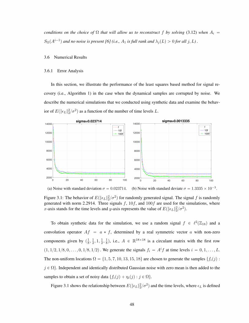
conditions on the choice of Ω that will allow us to reconstruct f by solving (3.12) when Ai “
SΩpAi´1q and no noise is present [6] (i.e., A1 is full rank and λjpLq ą 0 for all j, L) .
3.6 Numerical Results
3.6.1 Error Analysis
In this section, we illustrate the performance of the least squares based method for signal re-
covery (i.e., Algorithm 1) in the case when the dynamical samples are corrupted by noise. We
describe the numerical simulations that we conducted using synthetic data and examine the behav-
ior of EpεL22σ2q as a function of the number of time levels L.
0 20 40 60 80 100
2000
4000
6000
8000
10000
12000
14000
sigma=0.023714
f
10f
100f
(a) Noise with standard deviation σ “ 0.023714.
0 20 40 60 80 100
2000
4000
6000
8000
10000
12000
14000
sigma=0.0013335
f
10f
100f
(b) Noise with standard deviate σ “ 1.3335ˆ 10´3.
Figure 3.1: The behavior of EpεL22σ2q for randomly generated signal. The signal f is randomly
generated with norm 2.2914. Three signals f , 10f , and 100f are used for the simulations, wherex-axis stands for the time levels and y-axis represents the value of EpεL22σ
2q.
To obtain synthetic data for the simulation, we use a random signal f P `2pZ18q and a
convolution operator Af “ a ˚ f , determined by a real symmetric vector a with non-zero
components given by p18 ,
12 , 1,
12 ,
18q, i.e., A P R18ˆ18 is a circulant matrix with the first row
p1, 12, 18, 0, . . . , 0, 18, 12q . We generate the signals fi “ Aif at time levels i “ 0, 1, . . . , L.
The non-uniform locations Ω “ t1, 5, 7, 10, 13, 15, 18u are chosen to generate the samples tfipjq :
j P Ωu. Independent and identically distributed Gaussian noise with zero mean is then added to the
samples to obtain a set of noisy data tfipjq ` ηipjq : j P Ωu.
Figure 3.1 shows the relationship between EpεL22σ2q and the time levels, where εL is defined
48

0 2 4 6 8 10 12 14 16 18-2
0
2
4
6
8
10
12
14
error with sigma=0.023714, norm of signal is 22.9143
recovered signal
original signal
(a)
0 2 4 6 8 10 12 14 16 180
1
2
3
4
5
6
7
8error with sigma=0.023714, norm of signal is 22.914
recovered signal
original signal
(b)
0 2 4 6 8 10 12 14 16 180
20
40
60
80
100
120
140error with sigma=0.023714, norm of signal is 229.143
recovered signal
original signal
(c)
0 2 4 6 8 10 12 14 16 180
10
20
30
40
50
60
70
80error with sigma=0.023714, norm of signal is 229.14
recovered signal
original signal
(d)
Figure 3.2: The original signals and the reconstructed signals are represented by blue circles andred stars, respectively. The signals in 3.2c and 3.2d are obtained from the signals in 3.2a and 3.2b,respectively, by multiplying by 10. The norm of the original signal in 3.2a equals the norm of theoriginal signal in 3.2b, the same is true for the signals in 3.2c and 3.2d.
49

by (3.13). For each L, the simulation was repeated 100 times with the same distribution of noise,
and EpεL22σ2q was estimated by averaging the 100 values of εL22σ
2. Figure 3.1a shows how
EpεL22σ
2q changes as L varies for three different signals: f , 10f , and 100f , where the noise
variance is σ “ 2.3714ˆ10´2 and the 2-norm of f approximately equals 2.2914. The graph of 10f
is given in Figure 3.2a. Figure 3.1b shows the behavior of EpεL22σ2q for the same signals as in
Figure 3.2a, where the noise variance is σ “ 1.3335ˆ 10´3. As shown in Figure 3.1, EpεL22σ2q
decreases as n increases and approaches the constant predicted by Theorem 3.5.3.
0 10 20 30 40 50 60 70 80 90 100
2000
4000
6000
8000
10000
12000
14000
sigma=0.023714
f
10f
100f
(a)
0 10 20 30 40 50 60 70 80 90 100
1000
2000
3000
4000
5000
6000
7000
8000sigma=0.023714
f
10f
100f
(b)
Figure 3.3: The behavior of EpεL22σ2q are shown in (3.3a) and (3.3b) for the sparsely supported
signals without and with applying the threshold method, respectively, where the samples are cor-rupted by Gaussian noise with zero mean and standard deviation 2.3714ˆ 10´2.
Figure 3.2 depicts the graphs of the reconstructed signals and the original signals 10f , 100f ,
10g, and 100g in Figures 3.2a, 3.2c, 3.2b, and 3.2d, respectively, where f, g P R18 are randomly
generated and scaled to the norm 2.2914. The reconstructed signals from the noisy data and the
original signals are shown in Figure 3.2a for 10f , in Figure 3.2b for 10g, in Figure 3.2c for 100f ,
and in Figure 3.2d for 100g, respectively. The noisy data are corrupted by Gaussian noise with zero
mean and standard deviation 2.3714 ˆ 10´2. As displayed in Figure 3.2, while the reconstructed
signals in Figures 3.2a and 3.2b are clearly different from the original signals, it is hard to distinguish
the reconstructed signals from the original signals in Figures 3.2c and 3.2d because the reconstructed
signals are very close to the original signals.
Figures 3.3 and 3.4 are simulation results for the sparsely supported signals. For these spe-
cial signals, a threshold method [50] is introduced for the samples and reconstructed signals. The
method is implemented as follows. Let the threshold T be 2σ, let y denote the sample vector, and let
50

0 2 4 6 8 10 12 14 16 18-2
0
2
4
6
8
10
12error with sigma=0.023714, norm of signal is 17.3205
recovered signal
original signal
(a)
0 2 4 6 8 10 12 14 16 18-2
0
2
4
6
8
10
12error with sigma=0.023714, norm of signal is 17.3205
recovered sparse signal
original sparse signal
(b)
Figure 3.4: A comparison of the reconstruction results before and after applying the thresholdmethod. (3.4a) and (3.4b) show the reconstruction results before and after applying the thresh-old method, respectively. In (3.4a) and (3.4b), the original signals have the same sparse supportt8, 9, 10u. The samples are corrupted by the independent Gaussian noise with mean 0 and standarddeviation 2.3714ˆ 10´2.
f 7L be the reconstructed signal. If |ypiq| ď T , we set ypiq “ 0, where ypiq is the i-th component of y.
Similarly, if |f 7Lpiq| ď T , we set f 7Lpiq “ 0. Then the reconstruction results before and after apply-
ing the threshold method are compared. Figures 3.3 and 3.4 illustrate the behavior of EpεL22σ2q
and the reconstructed signals before and after applying the threshold method, respectively. In the
simulation, the samples are corrupted by Gaussian noise with zero mean and standard deviation
2.3714 ˆ 10´2. A sparsely supported signal f P R18 is generated with support in the locations
t8, 9, 10u with fp8q “ fp9q “ fp10q “ 1. The MSE EpεL22σ2q are estimated for signals f , 10f ,
and 100f separately. As shown in Figure 3.3, for n sufficiently large, EpεL22σ2q is about 20%
smaller after the threshold method is applied to the samples and reconstructed signals. Figure 3.4
shows the graphs of the original signal 10f and the reconstructed signal, which suggests that the
signal reconstructed by applying the threshold method is more accurate than the one reconstructed
without applying the threshold method in the locations outside the support of the original signal.
These observations suggest that the threshold method can reduce EpεL22σ2q by improving the
accuracy of the zero sets.
51

3.6.2 Cadzow Denoising
In this section, we describe the impact of the Cadzow denoising technique described in Section
3.4 on dynamical sampling using synthetic data.
3.6.2.1 Denoising of the sampled data
We use a symmetric convolution operator A with eigenvalues t18, 14, 38, 12, 58, 34,
78, 1u. We let A act on the normalized randomly generated signal f “ p0.2931, 0.3258, 0.04568,
0.3286, 0.2275, 0.0351, 0.1002, 0.1967, 0.3444, 0.34710, 0.0567, 0.3492, 0.3443, 0.1746, 0.2879qT
iteratively for 100 times. The iterated signals are stored in a matrix Π as
Π “`
f Af A2f . . . A100f˘
“ pf0 f1 f2 . . . f100q
where Akf is a column vector for each 0 ď k ď 100 (see (3.1)). At each time level, the
generated signals are perturbed by i.i.d. Gaussian noise with zero mean and standard deviation
σ P t10´2, 10´3, 10´4, 10´5u; the noisy signals are denoted by
rΠ “ Π`H,
where Hi,j „ Np0, σ2q and every two entries of H are independent (see (3.2)).
The samples are taken uniformly on 3Z15 (i.e., m “ 3), specifically at locations Ω “
t1, 4, 7, 10, 13u. The Cadzow algorithm (Algorithm 3) is applied to the data rY “ SmΠ where
Sm is defined in the first paragraph of Section 3.3.3. The denoised data are denoted by Z which is
compared to SmΠ directly by computing
Z ´ SmΠ
SmΠ. (3.18)
In addition, the relative difference between the noisy data SmrΠ and SmΠ is computed as
SmrΠ´ SmΠ
SmΠ. (3.19)
The same process is repeated for 80 times (with the same Π and different H). The numerical
52
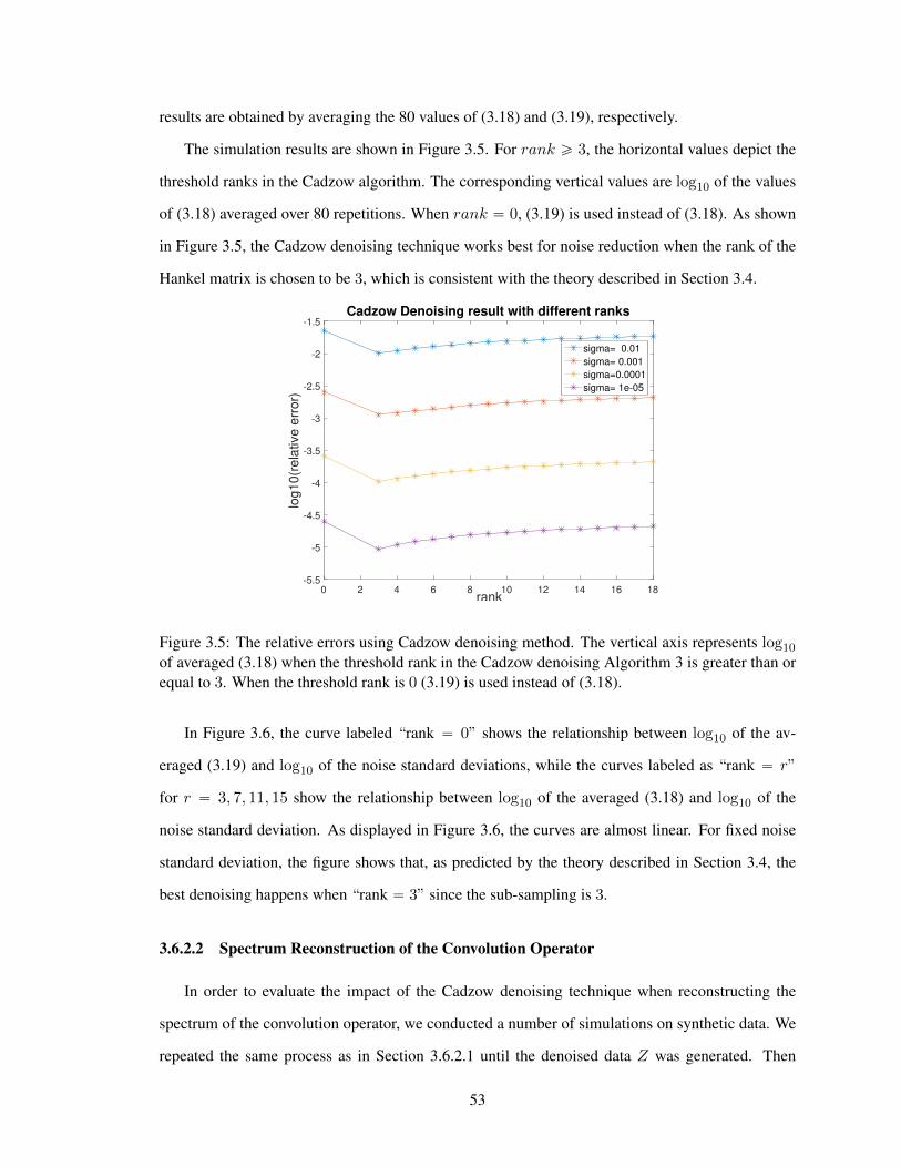
results are obtained by averaging the 80 values of (3.18) and (3.19), respectively.
The simulation results are shown in Figure 3.5. For rank ě 3, the horizontal values depict the
threshold ranks in the Cadzow algorithm. The corresponding vertical values are log10 of the values
of (3.18) averaged over 80 repetitions. When rank “ 0, (3.19) is used instead of (3.18). As shown
in Figure 3.5, the Cadzow denoising technique works best for noise reduction when the rank of the
Hankel matrix is chosen to be 3, which is consistent with the theory described in Section 3.4.
rank0 2 4 6 8 10 12 14 16 18
log
10
(re
lative
err
or)
-5.5
-5
-4.5
-4
-3.5
-3
-2.5
-2
-1.5Cadzow Denoising result with different ranks
sigma= 0.01
sigma= 0.001
sigma=0.0001
sigma= 1e-05
Figure 3.5: The relative errors using Cadzow denoising method. The vertical axis represents log10
of averaged (3.18) when the threshold rank in the Cadzow denoising Algorithm 3 is greater than orequal to 3. When the threshold rank is 0 (3.19) is used instead of (3.18).
In Figure 3.6, the curve labeled “rank “ 0” shows the relationship between log10 of the av-
eraged (3.19) and log10 of the noise standard deviations, while the curves labeled as “rank “ r”
for r “ 3, 7, 11, 15 show the relationship between log10 of the averaged (3.18) and log10 of the
noise standard deviation. As displayed in Figure 3.6, the curves are almost linear. For fixed noise
standard deviation, the figure shows that, as predicted by the theory described in Section 3.4, the
best denoising happens when “rank “ 3” since the sub-sampling is 3.
3.6.2.2 Spectrum Reconstruction of the Convolution Operator
In order to evaluate the impact of the Cadzow denoising technique when reconstructing the
spectrum of the convolution operator, we conducted a number of simulations on synthetic data. We
repeated the same process as in Section 3.6.2.1 until the denoised data Z was generated. Then
53

log10(sigma)-6 -5 -4 -3 -2 -1
log
10
(re
lative
err
or)
-7
-6
-5
-4
-3
-2
-1
0The relationship between the relative error and the noises
rank= 0
rank= 3
rank= 7
rank=11
rank=15
Figure 3.6: The relation between the relative errors and the noise standard deviations using theCadzow denoising method with different threshold ranks. The curves labeled “rank “ r”, r “3, 7 . . . reflect the relationship between log10 of the averaged relative errors and log10 of the noisestandard deviations, where the relative errors are represented in (3.18) for rank ě 3 and in (3.19)for rank “ 0.
54

we used the results of Section 3.3.3 and Algorithm 2 to recover the spectrum of the convolution
operator using separately denoised data Z and noisy data rY “ SmrΠ. The simulation results are
shown in Figures 3.7, 3.8, and 3.9 for different noise standard deviations. Figure 3.7 shows the
simulation results when the standard deviation of the noise is 10´5. The curves in Figure 3.7 are
simulation results for three different random choices of noise. For Figures 3.8 and 3.9, the noise has
standard deviations 10´4 and 10´3, respectively. As shown in Figures 3.7, 3.8, and 3.9, the Cadzow
denoising technique can make a big difference for the spectrum recovery.
Using the estimated convolution operator and the denoised data, we also evaluated the effective-
ness of the reconstruction algorithm, i.e., Algorithm 1, for which the simulation results are shown
in Figure 3.10. The figure shows that if the noise is small, the recovered signals are extremely close
to the original signals, which also verifies the effectiveness of the Cadzow denoising technique for
dynamical sampling.
3.6.3 Real data
In this section, we describe numerical tests that we performed using two sets of real data. One
data set documents a cooling process with a single heat source, and the other – a similar process with
two heat sources. These data sets were labeled as “one hotspot” and “two hotspots”, respectively.
The set-up for the real data sets is shown in Figure 3.11. We used the bicycle (aluminum) wheel
for the circular pattern. Fifteen (15) sensors are equidistantly placed around the perimeter of the
wheel with 4.5 inches apart. The specified accuracy of the sensors is 0.5˝C and the temperature
samples are taken at 1.05Hz.
The goal was to estimate the dynamical operator and the original signals by using information
from a subset of the thermometer measuring devices, while the totality of the measurements from all
devices was used as control to assess the performance of our estimations. In our reconstructions, we
did not use any a priori knowledge about the conducting material, its parameters, or the underlying
operator driving the evolution of the temperature. Only raw, time-space subsamples of the tem-
peratures was used to estimate the evolution operator, and the initial temperature distribution. The
operator was assumed to be real, symmetric convolution operator whose Fourier transform consists
of two monotonic pieces, so that recovery of the spectrum of the driving operator sufficed to recover
55

0 5 10 150.1
0.2
0.3
0.4
0.5
0.6
0.7
0.8
0.9
1sigma=1e-05
original eigenvalues
eigenvalues recovered from data with Cadzow
eigenvalues recovered from noised data
(a)0 5 10 15
0.1
0.2
0.3
0.4
0.5
0.6
0.7
0.8
0.9
1sigma=1e-05
original eigenvalues
eigenvalues recovered from data with Cadzow
eigenvalues recovered from noised data
(b)
0 5 10 150.1
0.2
0.3
0.4
0.5
0.6
0.7
0.8
0.9
1sigma=1e-05
original eigenvalues
eigenvalues recovered from data with Cadzow
eigenvalues recovered from noised data
(c)
Figure 3.7: A comparison of the spectrum reconstruction with and without the Cadzow denoisingtechnique for σ “ 10´5.
56

0 5 10 15-0.4
-0.2
0
0.2
0.4
0.6
0.8
1sigma=0.0001
original eigenvalues
eigenvalues recovered from data with Cadzow
eigenvalues recovered from noised data
(a)
0 5 10 15-0.4
-0.2
0
0.2
0.4
0.6
0.8
1sigma=0.0001
original eigenvalues
eigenvalues recovered from data with Cadzow
eigenvalues recovered from noised data
(b)
0 5 10 15-0.4
-0.2
0
0.2
0.4
0.6
0.8
1sigma=0.0001
original eigenvalues
eigenvalues recovered from data with Cadzow
eigenvalues recovered from noised data
(c)
Figure 3.8: A comparison of the spectrum reconstruction with and without the Cadzow denoisingtechnique for σ “ 10´4.
57

0 5 10 15-0.4
-0.2
0
0.2
0.4
0.6
0.8
1sigma=0.001
original eigenvalues
eigenvalues recovered from data with Cadzow
eigenvalues recovered from noised data
(a)
0 5 10 15-1.5
-1
-0.5
0
0.5
1sigma=0.001
original eigenvalues
eigenvalues recovered from data with Cadzow
eigenvalues recovered from noised data
(b)
0 5 10 15-0.5
0
0.5
1sigma=0.001
original eigenvalues
eigenvalues recovered from data with Cadzow
eigenvalues recovered from noised data
(c)
Figure 3.9: A comparison of the spectrum reconstruction with and without the Cadzow denoisingtechnique for σ “ 10´3.
58

0 5 10 150
0.05
0.1
0.15
0.2
0.25
0.3
0.35noise variance=1e-05
recovered signal
original signal
(a)
0 5 10 15-0.05
0
0.05
0.1
0.15
0.2
0.25
0.3
0.35
0.4noise variance=0.0001
recovered signal
original signal
(b)
0 5 10 15-0.1
-0.05
0
0.05
0.1
0.15
0.2
0.25
0.3
0.35
0.4noise variance=0.001
recovered signal
original signal
(c)
Figure 3.10: A comparison of the recovered signal and the original signal by using the estimatedrecovered convolution operator.
59

Figure 3.11: Set-up.
the filter.
In the experiment, the signal at time level 20 was set as the original state. First, we smoothed
the data by averaging over time to obtain a new data set Γ “ pγ1 γ2 . . .q, where γ1 “ř10i“1 fi,
γ2 “ř20i“11 fi, etc. Next, we extracted the information from the new data set at uniform locations
Ω with gap m “ 3 generating the data set SmpΓq. Cadzow Algorithm 3 is then used on rY “ SmpΓq
with the threshold rank close to 2 or 3 to obtain the denoised data Z. Using the data Z, Algorithm
2 was applied to estimate the filter. Finally, using the recovered filter, the original signals were
estimated by repeating the computations as in Section 3.6.1.
The test results on the data set with one hotspot are shown in Figure 3.12. Figure 3.12a depicts
the evolved signals at all 15 locations. Figure 3.12b shows the recovered spectrum of the evolution
filter using the data from locations Ω “ t1, 4, 7, 10, 13u to estimate the filter driving the system.
Using the driving operatorA recovered from Ω and the necessary extra sampling locations at t3, 15u
needed to recover the signal (Ωe “ ΩY t3, 15u) (see [7]), we reconstructed an approximation f 7 of
the signal that is displayed in Figure 3.12c; it has a relative error γ1´f72
γ12of 9.94% compared to the
60

actual measurements at all 15 locations as the reference. This relative error shows that dynamical
sampling also works reasonably well for a real data set.
0 20 40 60 80 100 120
20
25
30
35
40
45
50
55
60
65
70
location= 1
location= 2
location= 3
location= 4
location= 5
location= 6
location= 7
location= 8
location= 9
location=10
location=11
location=12
location=13
location=14
location=15
(a)
0 5 10 15
0.8
0.82
0.84
0.86
0.88
0.9
0.92
0.94
0.96
0.98
1
Spectrum
(b)
0 5 10 1510
20
30
40
50
60
70
80
recovered signal
original signal
(c)
Figure 3.12: Simulation results for the data set with one hotspot. Here, (3.12a) plots the evolvedsignals, (3.12b) shows the recovered spectrum by using the data from partial locations, and (3.12c)sketches the recovered signal by using the recovered operator from partial locations and the sampledoriginal signal. The partial locations for recovering the operator are Ω “ t1, 4, 7, 10, 13u. Torecover the original signals, we use the data from locations Ωe “ t1, 3, 4, 7, 10, 13, 15u.
The test results using the data set with two hotspots are shown in Figure 3.13. Figure 3.13a plots
the evolved signals at the 15 locations. Figure 3.13b exhibits the recovered spectrum of the filter with
Ω “ t2, 5, 8, 11, 14u. Using the driving operator A recovered from Ω and the data from locations
Ωe “ t2, 3, 5, 8, 10, 11, 14u, we recovered an approximation of the signal that is displayed in Figure
3.13c. In this case, the relative error was 12.45% compared to the actual measurements at all 15
locations. Such relative error is generally considered acceptable in this kind of real applications.
By making similar tests with different choices of Ω and Ωe, we found that the relative errors
61

0 20 40 60 80 100 120
20
30
40
50
60
70
80
location= 1
location= 2
location= 3
location= 4
location= 5
location= 6
location= 7
location= 8
location= 9
location=10
location=11
location=12
location=13
location=14
location=15
(a)
0 5 10 15
0.65
0.7
0.75
0.8
0.85
0.9
0.95
1
Spectrum
(b)
0 5 10 1520
30
40
50
60
70
80
recovered signal
original signal
(c)
Figure 3.13: Simulation results for the data set with two hotspots. Here, (3.13a) plots the evolvedsignals, (3.13b) shows the recovered spectrum by using the data from partial locations, and (3.13c)sketches the recovered signal by using the recovered operator from partial locations and the sampledoriginal signal. The partial locations for recovering the operator are Ω “ t2, 5, 8, 11, 14u. Torecover the original signals, we use the data from locations Ωe “ t2, 3, 5, 8, 10, 11, 14u.
62

0 5 10 15
0.86
0.88
0.9
0.92
0.94
0.96
0.98
1
Spectrum
(a)
0 5 10 1510
20
30
40
50
60
70
recovered signal
original signal
(b)
Figure 3.14: Simulation results for the data set with one hotspot. Here, (3.14a) shows the recoveredspectrum by using the data from partial locations, while (3.14b) plots the recovered signal by usingthe recovered operator from partial locations, where the partial locations for recovering the operatorare Ω “ t2, 5, 8, 11, 14u. To recover the original signals, we use the samples from locations Ωe “
t2, 3, 5, 8, 10, 11, 14u.
depend heavily on the choice of locations. The two pictures in Figure 3.14 are the results of the
same process that was used to generate the last two pictures in Figure 3.12. In this case, however,
we chose Ω “ t2, 5, 8, 11, 14u and Ωe “ t2, 3, 5, 8, 10, 11, 14u. This choice resulted in the relative
error of 34.29% which is considerably larger than the 9.94% in Figure 3.12.
3.7 Concluding remarks
This chapter introduces the problem of noise into the modeling of dynamical sampling and
discusses certain unbiased linear estimators for the recovery of signals from dynamical sampling.
The addition of noise to the model highlights some of the difficulties in recovering a signal from
measurements in dynamical sampling, and sets the stage for more detailed studies of the information
theoretic bounds and other types of estimators.
In addition, this chapter studies a special case related to blind deconvolution, where the subsam-
pling is uniform (to which extra samples are added for the recovery of the unknown signal), and
the evolution operator is unknown, but is one dimensional, symmetric, real and decreasing in the
frequency domain. The existence of multiple measurements over time, along with the assumptions
on the properties of the filter, allow for the recovery of the unknown signal and unknown filter; we
63

point to some of the factors that have an adverse effect on the stability of this procedure.
The basic algorithms and discussion of certain special cases are presented here with the intent
of providing a starting point for future work on both the theoretical and algorithmic aspects of noisy
instances of dynamical sampling and the case where the evolution operator is unknown.
64

Appendix A
Appendix for Chapter 3
A.1 Appendix for Proposition 3.5.1
Proof of Proposition 3.5.1. It is clear that
εL22 “
›
›
›
›
›
›
˜
Lÿ
i“1
A˚iAi
¸´1 ˜ Lÿ
j“1
A˚j ηj
¸
›
›
›
›
›
›
2
2
“
Lÿ
j“1
›
›
›
›
›
›
˜
Lÿ
i“1
A˚iAi
¸´1
A˚j ηj
›
›
›
›
›
›
2
2
`ÿ
j‰k
C˜
Lÿ
i“1
A˚iAi
¸´1
A˚j ηj ,
˜
Lÿ
i“1
A˚iAi
¸´1
A˚kηk
G
.
Since ηj and ηk for j ‰ k are independent and mean zero, the cross terms cancel out in expectation,
and one has
E
¨
˝
C˜
Lÿ
i“1
A˚iAi
¸´1
A˚j ηj ,
˜
Lÿ
i“1
A˚iAi
¸´1
A˚kηk
G
˛
‚“ 0.
Consequently,
EpεL22q “
Lÿ
j“1
E
¨
˝
›
›
›
›
›
›
˜
Lÿ
i“1
A˚iAi
¸´1
A˚j ηj
›
›
›
›
›
›
2
2
˛
‚. (A.1)
Note that
›
›
›
›
›
›
˜
Lÿ
i“1
A˚iAi
¸´1
A˚j ηj
›
›
›
›
›
›
2
2
“
›
›
›
›
›
›
˜
Lÿ
i“1
A˚iAi
¸´1 mjÿ
l“1
A˚plqj ηlj
›
›
›
›
›
›
2
2
“
mjÿ
l“1
›
›
›
›
›
›
˜
Lÿ
i“1
A˚iAi
¸´1
A˚plqj ηlj
›
›
›
›
›
›
2
2
`ÿ
l‰p
C˜
Lÿ
i“1
A˚iAi
¸´1
A˚plqj ηlj ,
˜
Lÿ
i“1
A˚iAi
¸´1
A˚ppqj ηpj
G
,
65

where A˚plqj denotes the l-th column of matrix A˚j and ηlj is the l-th entry of ηj . Additionally, ηlj and
ηpj are independent for l ‰ p. It follows that
E
¨
˝
C˜
Lÿ
i“1
A˚iAi
¸´1
A˚plqj ηlj ,
˜
Lÿ
i“1
A˚iAi
¸´1
A˚ppqj ηpj
G
˛
‚“ 0.
Thus,
EpεL22q “
Lÿ
j“1
mjÿ
l“1
E
¨
˝
›
›
›
›
›
›
˜
Lÿ
i“1
A˚iAi
¸´1
A˚plqj ηlj
›
›
›
›
›
›
2
2
˛
‚
“ σ2Lÿ
j“1
mjÿ
l“1
›
›
›
›
›
›
˜
Lÿ
i“1
A˚iAi
¸´1
A˚plqj
›
›
›
›
›
›
2
2
“ σ2 ¨
Lÿ
j“1
trace
¨
˝Aj
˜
Lÿ
i“1
A˚iAi
¸´2
A˚j
˛
‚
“ σ2 ¨ trace
¨
˝
˜
Lÿ
j“1
A˚jAj
¸˜
Lÿ
i“1
A˚iAi
¸´2˛
‚
“ σ2 ¨ trace
¨
˝
˜
Lÿ
i“1
A˚iAi
¸´1˛
‚“ σ2dÿ
i“1
1λipLq (A.2)
and the proposition is proved.
66

BIBLIOGRAPHY
[1] R. Aceska, A. Aldroubi, J. Davis, and A. Petrosyan. Dynamical sampling in shift invariant
spaces. In Azita Mayeli, Alex Iosevich, Palle E. T. Jorgensen, and Gestur Olafsson, editors,
Commutative and Noncommutative Harmonic Analysis and Applications, volume 603 of Con-
temp. Math., pages 139–148. Amer. Math. Soc., Providence, RI, 2013.
[2] R. Aceska and Y.H. Kim. Scalability of frames generated by dynamical operators. Frontiers
in Applied Mathematics and Statistics, 3, nov 2017.
[3] B. Adcock and A.C. Hansen. A generalized sampling theorem for stable reconstructions in
arbitrary bases. Journal of Fourier Analysis and Applications, 18(4):685–716, feb 2012.
[4] A. Aldroubi, A. Baskakov, and I. Krishtal. Slanted matrices, Banach frames, and sampling. J.
Funct. Anal., 255(7):1667–1691, 2008.
[5] A. Aldroubi, C. Cabrelli, A.F. Cakmak, U. Molter, and A. Petrosyan. Iterative actions of
normal operators. Journal of Functional Analysis, 272(3):1121–1146, 2017.
[6] A. Aldroubi, C. Cabrelli, U. Molter, and S. Tang. Dynamical sampling. Applied and Compu-
tational Harmonic Analysis, 42(3):378–401, 2017.
[7] A. Aldroubi, J. Davis, and I. Krishtal. Dynamical sampling: time-space trade-off. Appl.
Comput. Harmon. Anal., 34(3):495–503, 2013.
[8] A. Aldroubi and K. Grochenig. Nonuniform sampling and reconstruction in shift-invariant
spaces. SIAM Rev., 43(4):585–620 (electronic), 2001.
[9] A. Aldroubi, L.X. Huang, I. Krishtal, and R. Lederman. Dynamical sampling with random
noise. In Sampling Theory and Applications (SampTA), 2017 International Conference on,
pages 409–412. IEEE, 2017.
[10] A. Aldroubi, L.X. Huang, I. Krishtal, R. Lederman, A. Ledeczi, and P. Volgyesi. Dynamical
sampling with additive random noise. Sampling Theory in Signal and Image Processing, To
appear.
67

[11] A. Aldroubi, L.X. Huang, and A. Petrosyan. Frames induced by the action of continuous
powers of an operator. arXiv preprint, 2018.
[12] A. Aldroubi and I. Kryshtal. Krylov subspace methods in dynamical sampling. Sampling
Theory in Signal and Image Processing, Shannon Centennial Volume, 15:9–20, 2016.
[13] A. Aldroubi and A. Petrosyan. Dynamical sampling and systems from iterative actions of
operators. In Frames and other bases in abstract and function spaces, Appl. Numer. Harmon.
Anal., pages 15–26. Birkhauser/Springer, Cham, 2017.
[14] S.T. Ali, J.P. Antoine, and J.P. Gazeau. Continuous frames in hilbert space. Annals of Physics,
222(1):1–37, feb 1993.
[15] S.T. Ali, J.P. Antoine, and J.P. Gazeau. Coherent States, Wavelets and Their Generalizations.
Springer New York, 2000.
[16] R.F. Bass and K. Grochenig. Relevant sampling of bandlimited functions. Illinois J. Math., to
appear, 2012.
[17] Ake Bjorck. A general updating algorithm for constrained linear least squares problems. SIAM
J. Sci. Statist. Comput., 5(2):394–402, 1984.
[18] O. Bratteli and P. Jorgensen. Wavelets through a looking glass. Applied and Numerical Har-
monic Analysis. Birkhauser Boston Inc., Boston, MA, 2002. The world of the spectrum.
[19] J.A. Cadzow. High performance spectral estimation—a new ARMA method. IEEE Trans.
Acoust. Speech Signal Process., 28(5):524–529, 1980.
[20] E.J. Candes, J.K. Romberg, and T.Tao. Stable signal recovery from incomplete and inaccurate
measurements. Communications on Pure and Applied Mathematics, 59(8):1207–1223, 2006.
[21] C.Cabrelli, U.Molter, V.Paternostro, and F.Philipp. Dynamical Sampling on Finite Index Sets.
ArXiv e-prints, February 2017.
[22] C. Cheng, Y. Jiang, and Q. Sun. Spatially distributed sampling and reconstruction. CoRR,
abs/1511.08541, 2015.
68

[23] O. Christensen. Frames and Bases. Applied and Numerical Harmonic Analysis. Birkhauser
Boston Inc., Boston, MA, 2008.
[24] O. Christensen and M. Hasannasab. An open problem concerning operator representations of
frames. ArXiv e-prints, May 2017.
[25] O. Christensen and M. Hasannasab. Operator representations of frames: boundedness, duality,
and stability. ArXiv e-prints, April 2017.
[26] J.B. Conway. Functions of One Complex Variable. Springer US, 1973.
[27] J.B. Conway. Subnormal operators, volume 51 of Research Notes in Mathematics. Pitman
(Advanced Publishing Program), Boston, Mass.-London, 1981.
[28] J.B. Conway. A course in functional analysis. Graduate Texts in Mathematics. Springer, 2
edition, 1994.
[29] I. Daubechies. Ten Lectures on Wavelets. Society for Industrial and Applied Mathematics, jan
1992.
[30] R. J. Duffin and A. C. Schaeffer. A class of nonharmonic Fourier series. Trans. Amer. Math.
Soc., 72:341–366, 1952.
[31] M. Fornasier and H. Rauhut. Continuous frames, function spaces, and the discretization prob-
lem. Journal of Fourier Analysis and Applications, 11(3):245–287, Apr 2005.
[32] D. Freeman and D. Speegle. The discretization problem for continuous frames. ArXiv e-prints,
November 2016.
[33] J.P. Gabardo and D. Han. Frames associated with measurable spaces. Advances in Computa-
tional Mathematics, 18(2/4):127–147, 2003.
[34] J. Gillard. Cadzow’s basic algorithm, alternating projections and singular spectrum analysis.
Stat. Interface, 3(3):335–343, 2010.
[35] G.H. Golub and C.F. Van Loan. Matrix computations. Johns Hopkins Studies in the Mathe-
matical Sciences. Johns Hopkins University Press, Baltimore, MD, fourth edition, 2013.
69

[36] K. Grochenig, J.L. Romero, J. Unnikrishnan, and M. Vetterli. On minimal trajectories for
mobile sampling of bandlimited fields. Appl. Comput. Harmon. Anal., 39(3):487–510, 2015.
[37] P.R. Halmos. Normal dilations and extensions of operators. Summa Brasil. Math., 2:125–134,
1950.
[38] C. Heil. Wavelets and frames. In Signal processing, Part I, volume 22 of IMA Vol. Math.
Appl., pages 147–160. Springer, New York, 1990.
[39] T.L. Kriete III. An elementary approach to the multiplicity theory of multiplication operators.
Rocky Mountain J. Math., 16(1):23–32, 1986.
[40] P. Jorgensen and F. Tian. Von Neumann indices and classes of positive definite functions.
Journal of Mathematical Physics, 55(9):093502, 2014.
[41] D. Kundur and D. Hatzinakos. Blind image deconvolution. IEEE signal processing magazine,
13(3):43–64, 1996.
[42] Y.M. Lu, P.L. Dragotti, and M. Vetterli. Localizing point sources in diffusion fields from spa-
tiotemporal measurements. In Proc. Int. Conf. Sampling Theory and applications (SampTA),
Singapore, 2011.
[43] Y.M. Lu and M. Vetterli. Spatial super-resolution of a diffusion field by temporal oversampling
in sensor networks. In Proc. IEEE International Conference on Acoustics, Speech and Signal
Processing, number LCAV-CONF-2009-009, pages 2249–2252, 2009.
[44] A.W. Marcus, D.A. Spielman, and N. Srivastava. Interlacing families II: Mixed characteristic
polynomials and the Kadison-Singer problem. Ann. of Math. (2), 182(1):327–350, 2015.
[45] J. Murray-Bruce and P.L. Dragotti. Estimating localized sources of diffusion fields using
spatiotemporal sensor measurements. IEEE Trans. Signal Process., 63(12):3018–3031, 2015.
[46] J. Murray-Bruce and P.L. Dragotti. A sampling framework for solving physics-driven inverse
source problems. IEEE Transactions on Signal Processing, 65(24):6365–6380, Dec 2017.
70

[47] M. Zuhair Nashed. Inverse problems, moment problems, signal processing: un menage a
trois. In Mathematics in science and technology, pages 2–19. World Sci. Publ., Hackensack,
NJ, 2011.
[48] F. Philipp. Bessel orbits of normal operators. Journal of Mathematical Analysis and Applica-
tions, 448(2):767 – 785, 2017.
[49] J. Ranieri, A. Chebira, Y.M. Lu, and M. Vetterli. Sampling and reconstructing diffusion fields
with localized sources. In Acoustics, Speech and Signal Processing (ICASSP), 2011 IEEE
International Conference on, pages 4016–4019, May 2011.
[50] J.A. Rice. Mathematical Statistics and Data Analysis. Duxbury Advanced Series. 3 edition,
2007. ISBN 0-534-39942-8.
[51] W. Rudin. Real and Complex Analysis. International Series in Pure and Applied Mathematics.
McGraw-Hill Science/Engineering/Math, 3 edition, 1986.
[52] W. Rudin. Functional Analysis. International Series in Pure and Applied Mathematics.
McGraw-Hill Science/Engineering/Math, 2 edition, 1991.
[53] T. Strohmer. Finite- and infinite-dimensional models for oversampled filter banks. In Modern
sampling theory, Appl. Numer. Harmon. Anal., pages 293–315. Birkhauser Boston, Boston,
MA, 2001.
[54] Q. Sun. Nonuniform average sampling and reconstruction of signals with finite rate of inno-
vation. SIAM J. Math. Anal., 38(5):1389–1422 (electronic), 2006/07.
[55] J. Wermer. On invariant subspaces of normal operators. Proc. Amer. Math. Soc., 3:270–277,
1952.
[56] Q. Zhang, R. Li, and B. Liu. Periodic nonuniform dynamical sampling in `2pZq and shift-
invariant spaces. Numerical Functional Analysis and Optimization, 38(3):395–407, 2017.
[57] Q. Zhang, B. Liu, and R. Li. Dynamical sampling in multiply generated shift-invariant spaces.
Applicable Analysis, 96(5):760–770, 2017.
71