dynamical phase diagram of ultracold josephson junctions
TRANSCRIPT

PAPER • OPEN ACCESS
Dynamical phase diagram of ultracold Josephson junctionsTo cite this article: K Xhani et al 2020 New J. Phys. 22 123006
View the article online for updates and enhancements.
This content was downloaded from IP address 193.52.23.162 on 17/05/2021 at 11:30

New J. Phys. 22 (2020) 123006 https://doi.org/10.1088/1367-2630/abc8e4
OPEN ACCESS
RECEIVED
26 July 2020
REVISED
17 October 2020
ACCEPTED FOR PUBLICATION
9 November 2020
PUBLISHED
7 December 2020
Original content fromthis work may be usedunder the terms of theCreative CommonsAttribution 4.0 licence.
Any further distributionof this work mustmaintain attribution tothe author(s) and thetitle of the work, journalcitation and DOI.
PAPER
Dynamical phase diagram of ultracold Josephson junctions
K Xhani1,2,3,∗ , L Galantucci1 , C F Barenghi1 , G Roati2,3 , A Trombettoni4,5 andN P Proukakis1
1 Joint Quantum Centre (JQC) Durham-Newcastle, School of Mathematics, Statistics and Physics, Newcastle University, Newcastleupon Tyne NE1 7RU, United Kingdom
2 European Laboratory for Non-Linear Spectroscopy (LENS), Universita di Firenze, 50019 Sesto Fiorentino, Italy3 Istituto Nazionale di Ottica del Consiglio Nazionale delle Ricerche (CNR-INO), 50019 Sesto Fiorentino, Italy4 Department of Physics, University of Trieste, Strada Costiera 11, I-34151 Trieste, Italy5 CNR-IOM DEMOCRITOS Simulation Center and SISSA, Via Bonomea 265, I-34136 Trieste, Italy∗ Author to whom any correspondence should be addressed.
E-mail: [email protected] and [email protected]
Keywords: Josephson junction, superfluid quantum transport, dissipation, self-trapping, vortex rings, sound waves
AbstractWe provide a complete study of the phase diagram characterising the distinct dynamical regimesemerging in a three-dimensional Josephson junction in an ultracold quantum gas. Consideringtrapped ultracold superfluids separated into two reservoirs by a barrier of variable height andwidth, we analyse the population imbalance dynamics following a variable initial populationmismatch. We demonstrate that as the chemical potential difference is increased, the systemtransitions from Josephson plasma oscillations to either a dissipative (in the limit of low andnarrow barriers) or a self-trapped regime (for large and wider barriers), with a crossover betweenthe dissipative and the self-trapping regimes which we explore and characterize for the first time.This work, which extends beyond the validity of the standard two-mode model, connects the roleof the barrier width, vortex rings and associated acoustic emission with different regimes of thesuperfluid dynamics across the junction, establishing a framework for its experimentalobservation, which is found to be within current experimental reach.
1. Introduction
The Josephson effect is a direct manifestation of the macroscopic quantum phase coherence. Firstinvestigated in superconductors [1–3] and helium superfluids [4], Josephson effects have also been studiedfor exciton-polariton condensates in semiconductors [5, 6] and in dilute quantum gases, where the weakcoupling between spatially separated parts can be tuned by controlling the intensity of the energy barrierbetween them both for ultracold bosons [7–14] and fermions [15–19]. In the context of ultracold atoms,one can also realize Josephson junctions coupling two internal states via a weak driving field [20–23]. TheJosephson effect is crucially used for high-precision measurements, a major example being themeasurement of magnetic fields with superconducting quantum interference devices (SQUID) [24]. Thecontrol of ultracold atomic matter has given rise to the investigation towards analogous ‘atomtronic’applications, such as the atomtronic analogue of SQUID, termed AQUID [25–27], leading to a plethora ofstudies of weak link dynamics across diverse geometries and dimensionalities (see e.g. [28, 29] andreferences therein).
In Josephson junctions implemented with ultracold atoms (often referred to as ultracold Josephsonjunctions), the Josephson current can be driven by a chemical potential difference across the junction.Unlike superconducting Josephson junctions, in their ultracold counterparts, even in the absence of anyexternal chemical potential difference, a finite chemical potential difference can be present due to nonlinearinteractions and for a non-zero fractional population imbalance z = ΔN/N, where ΔN is the differencebetween the number of atoms in the two wells and N is the total number. Such population imbalance is atypical parameter used to characterise ultracold Josephson junction dynamics [30–32]. In fact, when the
© 2020 The Author(s). Published by IOP Publishing Ltd on behalf of the Institute of Physics and Deutsche Physikalische Gesellschaft
New J. Phys. 22 (2020) 123006 K Xhani et al
initial fractional population imbalance z0 is smaller than a critical value the system enters the well-known‘plasma’ Josephson oscillations regime, featuring periodic oscillations of both relative population imbalanceand relative phase about zero. When z0 instead becomes larger than a characteristic critical value, z is nolonger able to reach the zero value, with a bias towards the initially more populated well, such that the signof the relative population imbalance remains unchanged in time, despite the existence of low amplitudepopulation transfer across the weak link. This regime is known as a self-trapping regime [30] and it ischaracterised by a ‘running’ relative phase (i.e. a relative phase which grows with time). The occurrence ofthe self-trapping regime and an estimate of the critical fractional population imbalance [30] can be easilyobtained for a Bose–Einstein condensate (BEC) in a double-well potential by writing a two-mode modelstarting from the mean field Gross–Pitaevskii description. Notice that in general, for long times, theself-trapped regime is eventually destroyed by thermal or quantum fluctuations [31, 33–38] and/or byhigher order tunnelling processes [39].
Both these regimes, discussed for ultracold bosons in double- and multi-well potentials [30–32, 40],have been clearly observed both in ultracold 87Rb [8] and 39K [13] bosonic atomic clouds trapped in aharmonic potential perturbed by a shallow optical lattice which creates a weak link across twowell-separated minima, and in the presence of a deep optical lattice [7, 9].
Recent experiments with fermionic 6Li have investigated these phenomena in an elongated fermionicsuperfluid across the BEC–BCS regime [15, 16]. The molecular BEC regime observed in such experimentshas a direct correspondence with the experiments in atomic BECs. One of the interesting findings of theexperiment [15, 16]—based on a thin Josephson junction—was the explicit observation (across the entireBEC–BCS regime) of a transition from Josephson ‘plasma’ oscillations to a dissipative regime withincreasing initial population imbalance—with no evidence of the existence of self-trapping found in theprobed parameter space. The reason for the presence of the dissipative regime, and the correspondingabsence of the self-trapped one, can be qualitatively understood by observing that entering the self-trappedregion from the Josephson one, the relative phase passes from oscillating around zero to running linearly intime, reaching therefore the π-value. Thus, the barrier region can be a seed for the creation of vortexexcitations. If such excitations remain confined below the barrier, one may expect self-trapping to takeplace, while in the opposite case such excitations may start to propagate in the bulk of the system, givingrise to dissipative mechanisms. Therefore one can expect that, at least for not too large values of z0, there arethree phases: Josephson plasma oscillation, self-trapping, and dissipative. We pause here to anticipate thatone of the main goals of the present paper is to give and clarify the full dynamical phase diagram, as afunction of the parameters of the system, such as the width of the barrier, or the anisotropy of the fullthree-dimensional (3D) confining potential. We will also show that, between the dissipative and theself-trapping regimes, there is an intermediate regime where the vortex rings do not propagate, but there isa propagation of sound waves giving rise to dissipation. Moreover, our analysis demonstrates that, forsufficiently high barriers, the dominant dissipation mechanism is not the propagation of the vortex ring perse, but instead the sound waves generated by the decaying vortex ring.
The transition from dissipationless to dissipative superflow is a fundamental topic in its own right,whose understanding and control are central to any potential Josephson junction applications toatomtronics. The emergence of dissipation across a Josephson junction is well-known in condensed-mattersystems [41], with such dissipative process in ultracold superfluids having a close analogue to phase slipsobserved in superfluid helium [42–44].
Phase slips in ultracold Josephson junctions have been analysed across different atomic geometries anddimensionalities [16, 45–49]. In a 3D system, our earlier work [49] characterized the critical populationimbalance for the occurrence of such a dissipationless to dissipative transition, directly attributed to thephase slip associated to the dynamical emergence of one (or more) vortex rings, and consequent acousticemission. Depending on the system parameters, such vortex rings may enter the bulk condensate outsidethe barrier region, with their subsequent propagating dynamics determined by an interplay of acousticemission, vortex–sound interactions, kinetic energy conservation and thermal dissipation [49].
Vortex rings have also been discussed in the context of self-trapping: specifically, Abad et al [50]numerically related the self-trapping regime to phase slips created by emergent vortex rings whichannihilate within the weak-link region (but outside the region of observable condensate density).Dissipative dynamics can thus be related to an emerging vortex ring propagating along the main axis of thejunction, and either dissipating within it, or having sufficient energy to overcome the axial Josephsonbarrier and thus enter and propagate within the bulk condensate. For completeness, we note that this is avery distinct physical process to the thermal-induced decay of self-trapping state observed in [12] andqualitatively reproduced numerically in [36].
The above theoretical studies, combined with the existence of several experimental studies of theJosephson effect in ultracold superfluids observing either a transition from the Josephson plasma oscillation
2

New J. Phys. 22 (2020) 123006 K Xhani et al
regime to self-trapping [8, 9, 13], or a transition from Josephson to a dissipative regime [15, 16, 49], raisesthe interesting question of what distinguishes between such transitions/regimes, and whether a particularexperimental set-up could be found that would allow for all three regimes to be observed upon carefulcontrol of the relevant parameters distinguishing between such physical regimes.
In this work, we construct such a full phase diagram clearly demonstrating the crossover betweenJosephson ‘plasma’, dissipative and self-trapping regimes in a 3D ultracold Josephson junction, uponcareful control of the parameters (height, width) of the barrier acting as the weak link. Specifically, we firstlyidentify the parameter regime for which self-trapping is expected to arise in an elongatedharmonically-confined geometry with a Gaussian barrier along the main trap axis (motivated by the LENSexperiment [15, 16] in the BEC limit), an important feat in its own right, since only Josephson anddissipative regimes have so far been found in such a geometry.
We then generalize our studies to an isotropic harmonic trap (i.e. spherical condensate), and explicitlyshow—beyond the expected Josephson ‘plasma’ and self-trapping regimes—the emergence of a dissipativeregime also in such a geometry. Our unequivocal demonstration of the existence of all three regimes(Josephson plasma, dissipative, self-trapped) in different 3D geometries subject to careful parameteroptimization paves the way for the experimental observation of such a complete phase diagram.
This paper is structured as follows: after briefly reviewing our methodology and parameter regime(section 2), we present in section 3 the complete Josephson junction dynamical phase diagram in terms ofbarrier height and width for an ultracold Josephson junction in an elongated 3D condensate. Analysing thecompressible and incompressible kinetic energy emission during the superflow, and the properties of thevortex rings—when emitted—we characterize the microscopic processes controlling the regime crossover,even in the absence of any thermal dissipation (section 4). We also demonstrate the generic nature of ourresults, by confirming their relevance in a 3D isotropic trap (section 5). Finally we discuss our findings inthe context of other related works and present our conclusions (section 6). Our detailed analysis issupplemented by appropriate appendices which provide further details into the intricate observed dynamicsand crossover regions, and the relevance of the usual two-mode model.
2. Methodology
The superfluid dynamics of a 3D ultracold bosonic Josephson junction is modelled by the Gross–Pitaevskiiequation (GPE) for the wavefunction ψ:
i�∂ψ(r, t)
∂t= − �
2
2M∇2ψ(r, t) + Vext(r)ψ(r, t) + g|ψ(r, t)|2ψ(r, t), (1)
where M is the particle mass and g denotes the particle s-wave interaction strength. The external trappingpotential Vext(r) used throughout this work is based on a combination of a harmonic trap and a Gaussianbarrier, leading to a double-well potential of the form:
Vext(x, y, z) =1
2M
(ωx
2x2 + ωy2y2 + ωz
2z2)+ V0e−2x2/w2
, (2)
where ωx,y,z are the trapping frequencies along the x, y and z directions, and the Gaussian barrier imprintedalong the x-direction has a height V0 and a 1/e2 width w.
We create an initial population imbalance, z(t = 0) ≡ z0, between the two wells by adding initially alinear potential −εx along the x direction, and solving the GPE in imaginary time in such a tilted potential.For simplicity we choose the initial phase difference, Δφ0, between the two wells to be zero. At t = 0, thelinear potential is instantaneously removed, and the resulting population dynamics
z(t) =NR(t) − NL(t)
N, (3)
is modelled by the time-dependent GPE, with NL (NR) denoting the condensate number in the left (right)reservoir, and N = NL + NR the total condensate number.
We consider two different geometries: (i) an elongated harmonic trap (with an aspect ratio ∼ 11), and(ii) an isotropic (spherical) harmonic trap.
The main analysis is conducted for the elongated trap, based on the parameters of references [15, 16]:specifically, we use the experimental trap frequencies ωx = 2π × 15 Hz, ωy = 2π × 187.5 Hz,ωz = 2π × 148 Hz, and a fixed particle number N = 60 000. The experimental atomic Josephson junctionwas realized by bisecting the superfluid into two weakly-coupled reservoirs by focussing onto the atomiccloud a Gaussian-shaped repulsive sheet of light of intensity V0 and a 1/e2 waist of 2.0 ± 0.2 μm, whilebeing homogeneous along the other two directions [15]. In the BEC regime, the width of such barrier is
3
New J. Phys. 22 (2020) 123006 K Xhani et al
approximately four times the superfluid coherence length. Here M = 2mLi, where mLi is the mass of a 6Liatom, and the interaction strength g = 4π�2aM/M corresponds to an effective scattering length between themolecules aM � 0.6a (which is tunable [51]), which corresponds to the molecular BEC side of theexperiment with 1/(kFa) � 4.6, where kF =
√2mEF/� is the Fermi wave-vector and a the interatomic
scattering length. More details on the experimental set-up can be found in reference [52]. The validity ofthe GPE description on the BEC side of the BCS–BEC crossover has been discussed in reference [16, 49]where it is shown that for our present parameters (1/(kFa) � 4.6) the GPE predictions agree withexperimental findings.
We will also consider a spherical geometry and fix for simplicity the isotropic trap frequency to that ofthe x-axis in the elongated experiments, i.e. ωx = ωy = ωz = 2π × 15 Hz, keeping the total moleculenumber again fixed to 60 000. In the elongated case, μ � 114�ωx and the healing lengthξ = �/
√2 μM � 0.067lx ∼ 0.5 μm, whereas in the spherical case μ � 17�ωx and ξ � 0.17lx � 1.3 μm.
The separation induced by the barrier, and thus the tunnelling energy across the two wells depends ontwo parameters: its height V0 and width w. Physically, it is useful to have them in their dimensionless ratiosV0/μ and w/ξ. The system exhibits different behaviour across the junction depending on whether V0 ismuch larger or smaller than the chemical potential.
In this work, we identify the different dynamical regimes across the Josephson junction byindependently varying both parameters V0/μ and w/ξ, thus ranging from the limit of narrow/low barriersto wide/high barriers. Firstly, we consider the effect of changing V0/μ ∈ [0.6, 2.1] for the fixed (thin)experimental barrier width w/ξ = 4 in the elongated trap. We then repeat our analysis in the sameelongated harmonic trap for a fixed value of V0/μ ∼ 1.2 and a variable barrier width in the range w/ξ ∈[4, 10].
To verify the generality of our findings, we also consider the spherical trap geometry with the samebarrier width w/ξ = 4, but a variable V0/μ ∈ [0.6, 1.8]. In all cases, the probed parameter space has beenchosen to be broad enough, in order to reveal—in the appropriate limits—the emergence of all threeregimes: Josephson ‘plasma’, dissipative and self-trapped regime.
Numerically, we solve the dimensionless form of the GPE, scaling position to the harmonic oscillatorlength along the x direction lx =
√�/Mωx, energies to the harmonic oscillator energy �ωx, with densities
thus scaled to l−3x and time in units of 1/ωx. In these units, equation (1) becomes:
i∂ψ(r, t)
∂t=
(−1
2∇2 + Vext + g|ψ(r, t)|2
)ψ(r, t), (4)
where g = g/(l3x�ωx). For our numerical simulations we use a numerical grid length [−24, 24] lx, [−4, 4] lx,[−4, 4] lx along the x, y and z directions respectively, and a number of grid points of 1024 × 128 × 128 forthe elongated trap. For the spherical trap we use a numerical grid length [−10, 10] lx along all threedirections, and a number of grid points 256 × 128 × 128, slightly biased towards the x axis for betterdetection of the vortex rings.
3. Dynamical regimes for the elongated trap
We start by analyzing the complete phase diagram of emerging dynamical regimes across a Josephsonjunction in an elongated 3D BEC, and demonstrate clearly the dynamical behaviour across those differentregimes, and also the crossover between them.
3.1. Dependence on barrier heightThe LENS experiment [15], conducted for a rather thin barrier w/ξ ∼ 4 and V0/μ � 1.2 observedundamped Josephson plasma oscillations and a transition to the dissipative regime. Motivated by theunexpected absence of the self-trapping regime—a regime well observed in other ultracold atomexperiments [8, 9, 13, 53]—we extended our numerical simulations to larger barrier heights. Our previouswork [49] had in fact shown that the analytical two-mode model [30]—on which the prediction ofself-trapping is based—does not give accurate results for V0/μ � 1.2. (A discussion of the validity of thetwo-mode model for the broader range V0/μ � 2.1 is shown in appendix A). Here, we extend ournumerical simulations also in the direction of increasing V0/μ, and indeed find for the consideredparameters the onset of the self-trapping regime for barrier height V0/μ� 1.6.
The full phase diagram highlighting the distinct dynamical regimes for a narrow barrier width w/ξ = 4is shown in figure 1. The central panel of figure 1 highlights the different ‘Josephson’, ‘dissipative’ and‘self-trapped’ regimes, and their crossover for barrier heights in the range [0.6, 2.1]μ. Subplots(i), (ii) [left panels] and (iii), (iv) [right] show characteristic dynamical evolution curves of the population
4

New J. Phys. 22 (2020) 123006 K Xhani et al
Figure 1. Main panel: Josephson junction phase diagram of dynamical regimes arising across a Gaussian barrier of variableheight V0/μ ∈ [0.6, 2.1] and fixed w/ξ = 4 for different initial fractional population imbalances z0 = z(t = 0). The Josephsonplasma oscillation regime dominates for z0 < zcr and, beyond a narrow transition regime (indicated by the grey shaded area) thesystem transitions to the dissipative (V0/μ � 1.2), or the self-trapped (V0/μ� 1.6) regime, with the empty black triangles (andconnected dashed black line) indicating the critical imbalance. Such regimes are characterized by the coloured regions displayingthe absolute value of 〈z(t)〉/z0 where 〈z(t)〉 is the temporal mean value of z(t) in the time interval [0, 0.4] s; the colormap is inlogarithmic scale ranging between 0.08 and 0.75. In the lateral figures we plot the evolution of the population imbalance z(t) fordifferent z0 and (i), (ii) V0/μ � 0.8 at w/ξ = 4, showing the transition from the Josephson ‘plasma’ oscillations to the dissipativeregime; and (iii), (iv) V0/μ = 2 at w/ξ = 4, showing the transition from the Josephson to the self-trapping regimes. Thelocation of such points on the phase diagram are highlighted by the hollow points (with the connecting white vertical linessimply a guide to the eye). The horizontal dot-dashed line at the top of the phase diagram indicates the value of z0 = 0.19 chosenfor the study of the vortex ring dynamics.
imbalance z(t) for increasing values of initial imbalance z0 and for fixed V0/μ � 0.8 [(i), (ii) Josephsonplasma to dissipative transition] and V0/μ = 2.0 [(iii), (iv) Josephson plasma to self-trapped transition];the location of the displayed cases is highlighted on the phase diagram by white hollow circles. Whileindividual transitions from either Josephson plasma to dissipative, or from Josephson plasma toself-trapped had been previously studied both numerically and experimentally, this is the first time that allthree regimes appear in a single phase diagram. Importantly, this is the first study displaying the gradualcrossover from dissipative to self-trapped regimes.
The procedure for constructing this phase diagram is as follows: for each value of the barrier heightwithin the chosen range [V0/μ] ∈ [0.6, 2.1] we vary (in small discrete steps) the initial imbalance z0 fromsmall enough values for which pure Josephson ‘plasma’ oscillations are observed, up to sufficiently highvalues z0 ∼ 0.19 and perform numerical evolution of the GPE to obtain the dynamical evolution of z(t) upto 400 ms. Such parameters have been chosen to ensure both that the range of initial conditions (values ofz0) is broad enough to facilitate the crossing of the relevant critical threshold, and that propagation occurson a sufficiently long timescale to clearly highlight the existence of such different dynamical regimes. Thecritical value zcr is itself identified as the point at which the system clearly transits to a regime distinct froma well-defined single-frequency oscillation in both relative population and phase (Josephson ‘plasma’regime). To better understand our numerical identification of zcr, it is convenient to consider twocharacteristic cases of sufficiently low (V0/μ = 0.8) and high (V0/μ = 2.0) barrier heights, for which thecorresponding transitions from Josephson ‘plasma’ to either dissipative, or self-trapped, have beenpreviously established (see e.g. [49] and references therein): the corresponding dynamical curves for thepopulations imbalance, z(t), are shown for increasing z0 in the left and right subplots of figure 1.
For V0/μ � 0.8 (left panels), increasing the initial population imbalance leads—for some value ofz0—to a dynamical evolution in which z(t) presents a single ‘kink’ during the first transfer cycle ofpopulation across the weak link. Such a kink is known to signal the generation of a single vortex ring whichtemporarily slows down (potentially even momentarily reversing) the evolution of z(t) [49], thus identifyingthis very distinct ‘dissipative’ regime of the population dynamics. In this limit—and following establishedprocedures [49]—the critical population imbalance zcr is defined as the value of z0 for which there is exactlyone kink in the initial decay of z(t) (before z(t) reaches the value of zero for the first time). This transition isclearly visualised by the change in the dynamical profile from the cyan (lower) plot exhibiting ‘plasma’oscillations, to the dark blue curve in figure 1(ii). In the opposite limit of larger barrier heights(V0/μ � 1.6), the increase of z0 from small values leads to a sudden transition from a Josephson regime ofsymmetric oscillations about a zero mean value, to a regime in which the population imbalance oscillates(undamped) around a non-zero mean value (as evident in figure 1 (right panels) for V0/μ = 2). In thislimit—and consistent with previous works [30]—we define the critical population imbalance, zcr, as the
5
New J. Phys. 22 (2020) 123006 K Xhani et al
first (lowest) value of z0 for which we detect such self-trapped oscillations. Between those two limits—andspecifically in the range 1.2 < V0/μ < 1.6—, zcr is identified as the lowest value of z0 (for a given V0/μ) atwhich the dynamical oscillations exhibit an irregular/non-periodic decay pattern. Examples cases—whichalso shed more light on the intermediate regime—are given in appendix B.
Although a critical population imbalance can be predicted by the commonly-used two-mode model, wenote that such an approach cannot be used in our system: this is because zcr in the two-mode model onlydefines the specific transition from a Josephson ‘plasma’ to a self-trapping state, and cannot facilitate theexistence of a dissipative regime. In fact, the two-mode model can only become relevant in our presentsetting for high V0/μ, with the detailed critical assessment given in appendix A confirming its restrictedvalidity to the range of barrier heights where the self-trapping is obtained.
For values of z0 clearly exceeding zcr, the system exhibits a more complicated excitation pattern, as alsoindicated by figures 1(i) and (iii): specifically, in the dissipative regime [subplot (i)], this leads to thesequential generation of multiple vortex rings (as visible by the multiple kinks), while in the self-trappedregime [subplot (iii)] this leads to multiple higher-frequency excitations, both of which are furthercharacterised later on. Interestingly, the ‘curved’ nature of the crossover from dissipative to self-trappedregime (observed here at fixed w/ξ) implies that for a given V0/μ value in the intermediate region, anincrease in z0 leads to a significant associated increase in the value of |〈z(t)〉|/z0.
The interplay between all such regimes poses challenges on how to best present the complete phasediagram. We have found that the best way to depict the physical regimes emerging for z0 � zcr is bycharacterising them in terms of the absolute value of 〈z(t)〉/z0, where 〈z(t)〉 denotes the temporal meanvalue of the population imbalance over our entire numerically probed range, which tends to values 0 and 1respectively deep in the dissipative and self-trapped regimes. Such a representation is plotted by colour infigure 1 (and similar subsequent figures). Our rationale for choosing such a classification is twofold: firstly,the (necessarily) limited temporal evolution window probed (0 � t � 0.4 s) implies a weak sensitivity ofcalculated values 〈z(t)〉 around a zero mean in the dissipative/crossover regime, making it more intuitive toconsider |〈z(t)〉|, as opposed to simply 〈z(t)〉. Secondly, given that in the self-trapped regime the populationimbalance oscillates about a non-zero value, and that the higher the value of z0 probed, the smaller theamplitude of oscillations, it is thus appropriate to scale the population imbalance to z0. Such arepresentation enables a gradual transition from |〈z(t)〉|/z0 ∼ 0 in the (deep) dissipative regime, to|〈z(t)〉|/z0 ∼ 1 in the deep self-trapped limit (high V0/μ and z0 � zcr).
Well below the line of critical population imbalances, the system behaviour is dominated by symmetricJosephson ‘plasma’ oscillations, with a single dominant frequency. Between the regime of such oscillationsand the critical population imbalance line, we have included a narrow grey band to indicate—within thelimitation of our discrete set of probed z0 values—an intermediate regime of more complicated transitionalbehaviour, where the system displays a clear deviation from Josephson ‘plasma’ oscillations with increasingz0: this can either exhibit some dissipative evolution but without a vortex ring being generated in the firstpopulation transfer cycle (although one may appear in later evolutionary stages) [low to intermediateV0/μ], or exhibit anharmonic oscillations or signs of unstable (short-time) self-trapping behaviour whichdecays in less than the probed 0.4 s [intermediate to high V0/μ]. Note that intermediate values of V0/μ
(broadly arising for our current parameters around 1.2 < V0/μ < 1.6, but also dependent on z0) are alsocharacterized by reduced sound emission, with any generated vortex rings remaining as ‘ghost’ vortices(i.e. without entering the condensate), and a complicated irregular pattern of population oscillations,during which z(t) may exhibit kinks, or can change sign, but in a sufficiently irregular manner that does notmeet the criteria for belonging to either of the three identified regimes. Further details on all such crossoverregions are discussed in appendix B, which includes (figure B2) characteristic population imbalanceevolution curves, z(t), across the range of probed V0/μ to more clearly illustrate how the system behaviourtransitions from Josephson, through the grey transition region, to the critical population imbalance andbeyond.
Having explained how we constructed the phase diagram and given an overview of the key observedfeatures—which cumulatively constitute the main result of this work—we now discuss in more detail thekey emerging features of the z(t) oscillations shown in figure 1.
Our presentation so far has focussed on the distinct nature of the z(t) oscillations alone. Although—aswill become evident below—this is highly characteristic of the type of dynamics exhibited by the system, itis nonetheless well-known that dynamics across a Josephson junction require parallel characterisation ofboth fractional population imbalance and relative phase. To further justify our presented physicalinterpretation, figure 2 shows in parallel characteristic examples of both the time-evolution of thepopulation imbalance and the corresponding relative phase for different z0, focussing on the limiting cases(a), (b) V0/μ � 0.8 and (c), (d) V0/μ = 2. The dynamics shown here correspond to a subset of plots fromfigure 1, selected so as to better characterise both relative population and phase oscillations over the time
6

New J. Phys. 22 (2020) 123006 K Xhani et al
Figure 2. The temporal evolution of the imbalance and the relative phase for (a), (b) V0/μ � 0.8 and for (c), (d) V0/μ = 2 fordifferent values of z0 and at fixed w/ξ = 4. (a) and (b) Shown are cases (a) z0 < zcr (cyan; Josephson ‘plasma’ regime), andz0 = zcr (dark blue, dissipative regime), and (b) z0 > zcr (purple, yielding multiple vortex ring generation). (c) and (d) Shown areself-trapped cases z0 = zcr (red) and z0 > zcr (maroon), revealing the emergence of multiple frequencies with increasing z0. Therelative phase is calculated along the line y = z = 0 near the trap centre, except for the inset of (b) where the relative phase iscalculated for z = 0, but y � 0.44lx. The vertical grey dashed lines show the time at which the population imbalance has the firstlocal minimum.
period where they occur (note the different z(t), Δφ and time axes selected to best capture the relevantbehaviour). The phase difference Δφ between the left and right reservoir is calculated here for y = z = 0and near the barrier (unless stated otherwise).
Specifically, figure 2(a) depicts both a characteristic evolution in the Josephson ‘plasma’ oscillationsregime (cyan), and the corresponding evolution at z0 = zcr (dark blue). As well-known, in the Josephson‘plasma’ regime both z(t) and Δφ(t) oscillate sinusoidally around the zero-value. In stark contrast, thepopulation imbalance at z0 = zcr exhibits a kink associated with vortex ring generation [figure 2(a), top], asfurther confirmed by the temporally coinciding 2π jump in the relative phase [figure 2(a), bottom].Increasing z0 further beyond zcr leads to the successive generation of multiple vortex rings, as visible by thethree consecutive kinks in both z(t) and Δφ(t) in figure 2(b). As the three vortex rings do not shrink to zeroat x = 0 (i.e. at the barrier centre) but they instead propagate in the left reservoir, (i.e. |x| � 2w), therelative phase does not jump by 2π around x = 0 [figure 2(b), bottom]; to see this instead requires therelative phase to be calculated at the appropriate non-zero value of y associated with the vortex ring core,which indeed yields jumps by almost 2π for y = 0.44lx (inset of figure 2(b), bottom).
Figure 2(c) depicts the established self-trapped regime typically discussed in the context of thetwo-mode model, and labelled as ‘macroscopic quantum self-trapping’, or MQST: in this regime, thepopulation imbalance exhibits regular periodic oscillations about a non-zero value, accompanied by 2πjumps in the relative phase at the times of the z(t) local minima, with a rate captured well by the two-modemodel (νMQST � Δμ/h � 12 Hz). In this work, we henceforth refer to this regime as the ‘pure’ self-trappedregime, in order to make a distinction to the dynamics observed for much higher initial populationimbalances.
Specifically, we find that as z0 increases to higher values (much beyond zcr), not only does the amplitudeof the oscillations decrease significantly, with its corresponding frequency significantly increasing, but thepattern becomes increasingly less regular: an example of this is shown in figure 2(d) [see also appendix B].The origin of this is the co-existence of multiple modes, corresponding to additional higher-level excitationsand complicated couplings [54, 55], which result in less regular dynamics than those discussed in the puretwo-mode self-trapping regime [30]. Nonetheless, closer inspection even in this regime, still reveals theexistence of (irregular) 2π phase jumps at the relative population minima, thus allowing us to stillcharacterise this regime as ‘self-trapped’ (depicted by the dark red colour in the various phase diagramsshown in this paper).
7

New J. Phys. 22 (2020) 123006 K Xhani et al
Figure 3. Josephson junction phase diagram of dynamical regimes arising across a Gaussian barrier of fixed V0/μ = 1.17 anddifferent values of the barrier widths in the range [4, 10]ξ. Other symbols have the same meaning as in figure 1.
Our analysis has clearly demonstrated, that all three dynamical regimes are accessible in a given (hereelongated 3D) geometry, for a given barrier width, by changing the barrier height. Changing the barrierheight naturally induces different behaviours around V0/μ ∼ O(1), due to the effective density across thebarrier. Of course, for a Gaussian barrier the junction properties depend on a combination of barrier heightand width, and so our results should be reproducible when fixing geometry and barrier height, butchanging width, as demonstrated below.
3.2. Dependence on barrier widthHere we repeat our study of the dynamical regimes in the same elongated 3D geometry, but for fixed barrierheight V0/μ = 1.17—which we would still class as belonging to the dissipative regime for w/ξ = 4(and z0 � zcr)—and different values of the barrier width compared to the healing length ξ. Thecorresponding results are shown in figure 3, and clearly reveal the same qualitative behaviour as foundabove.
When the width is narrow (w/ξ � 6), and for population imbalances z0 � zcr such that the systemtransitions away from the Josephson regime, the barrier acts more like a perturbing force to the initialsuperfluid flow, leading to significant acoustic energy emission and vortex ring(s) generation—with thesystem thus entering (in agreement with earlier findings) the dissipative regime. Increasing the barrierwidth at constant height, leads to a stronger effective barrier which isolates the two wells more, thusdecreasing the Josephson coupling energy EJ in comparison to the self-interaction energy (for fixed z0)ECz2
0N2/8: the system now transitions to the self-trapped regime. For small values z0 which only slightlyexceed zcr, the system finds itself in the pure self-trapped regime, with higher z0 leading to the morecomplicated self-trapped states discussed above.
3.3. Critical population imbalance phase diagramTo gain further insights on the generality of the results presented previously, we next investigate thedependence of the critical population imbalance, appropriately scaled densities and healing lengths whichdefine the transition from Josephson to the other (dissipative; self-trapped) dynamical regimes in terms ofboth barrier height V0/μ and barrier width w/ξ. This is shown in figure 4, and clearly characterizes the keyparameters in terms of the transition between dissipative and self-trapped regimes.
Specifically, figure 4(a) shows the value of the critical population imbalance, zcr —which is representedby the colour of the points—for each probed V0/μ and w/ξ combination.
In other words, each horizontal cut of figure 4(a) corresponds to tracing the actual critical populationimbalance line (z0 = zcr) at fixed w/ξ (as in figure 1), with the region between dashed blue and dashedorange lines in figure 4(a) indicating the crossover between dissipative and self-trapped regimes for eachbarrier height/width combination. Similarly, vertical cuts of figure 4(a) trace the critical populationimbalance line at fixed V0/μ (as in figure 3).
As a result, for each w/ξ, we can identify two distinct threshold values for V0 which characterize thedistinct dynamical regimes the system can exhibit when transitioning out of the Josephson regime withincreasing z0. The first (lower) threshold value, corresponding to any point on the dashed blue line, marks
8

New J. Phys. 22 (2020) 123006 K Xhani et al
Figure 4. (a) Alternative phase diagram in the V0/μ–w/ξ space of parameters depicting (a) the value of the critical populationimbalance, zcr, (b) the scaled density, and (c) the scaled inverse coherence length, as a function of V0/μ ∈ [0.6, 1.6] and w/ξ ∈[4, 10]. Their values are represented by the colorbar shown in logarithmic scale. For each value of w/ξ there exists a maximumvalue of the barrier height V = Vdissip (denoted by the dashed blue line) below which we find a pure dissipative regime at z0 ≈ zcr,and another value of the barrier height V = VMQST (denoted by the dashed orange line), above which the system transitions to aself-trapped regime, and specifically to a pure self-trapped regime for z0 ≈ zcr. The numerical data between the dark-blue and theorange lines correspond to the intermediate, or ‘crossover’, regime. In (b) the density at the trap centre is scaled to the maximumvalue of the density in the absence of the barrier, while in (c) the mean coherence length is correspondingly scaled to thecoherence length at the trap centre.
(for given μ) the maximum value of the barrier height, Vdissip, for which the system can exhibit thedissipative regime behaviour. Put differently, for all values of V0 � Vdissip (i.e. combinations of w/ξ andV0/μ lying on the left of the dashed blue line in figure 4(a)), the system is in a configuration facilitatingtransitions from Josephson to dissipative regime for z0 � zcr. The colour in this case labels the value of zcr
for which such a transition occurs. The second (upper) threshold, corresponding to any point on thedashed orange line, marks (for given μ) the minimum value of the barrier height, VMQST, for which thesystem can exhibit the self-trapped regime behaviour. This implies that for all values of V0 � VMQST
(i.e. combinations of w/ξ and V0/μ lying on the right of the dashed orange line in figure 4(a)), the systemis in a configuration facilitating transitions from Josephson to the self-trapped regime for z0 � zcr. The darkred colour seen here (corresponding to low values) reflects the fact that such a critical population imbalancevalue (zcr) is much lower than that found in the parameter space facilitating a transition to the dissipativeregime. The above analysis has thus allowed us to parametrize—for our studied parameter space—therange of values which place the system in the ‘intermediate’ regime between dissipative and self-trapped forz0 � zcr. Such crossover parameter regime is bounded by the dashed blue, and dashed orange lines.
Summarizing, the dissipative regime can be found (for z0 � zcr) both for relatively low and narrowbarriers, and for wider but low barriers, whereas self-trapping emerges at the other end of parameter space.Interestingly—for the range of the barrier widths explored—the system is in the dissipative regime forz0 = zcr independently on the value of w/ξ when V0/μ � 0.8, while at the other end for values V0/μ = 1.6the system enters the pure self-trapping regime independently of the value of w/ξ.
For the elongated experimental parameters references [15, 16] the critical population imbalance atwhich the interesting crossover dynamics emerges is rather low, placing strong constraints on itsexperimental observation. However, the actual value of zcr at such boundaries is very geometry-dependent,and we later show how an isotropic trap can significantly enhance the observable relevant region.
An important comment regarding figure 4(a) is that the value of zcr at which the transition to (pure)self-trapping takes place, i.e. along the transition line, is rather independent of the values of V0/μ and w/ξ.This also occurs, although to a lesser extent, along the dissipative transition line.
Interestingly, a similar qualitative picture emerges when looking at the value of the density at the trapcentre, scaled to its corresponding value in the absence of the barrier, i.e. n0/nmax. Another way to plot thisinformation is as the inverse of the ratio of the coherence length calculated at the trap centre to the meanvalue coherence length ξmean extracted by the maximum density in the absence of the barrier, i.e.(ξ0/ξmean)−1. These are respectively shown in figures 4(b) and (c). Such results suggest, along the lines ofthe preceeding discussion, that—for each value of w/ξ—two threshold values of n0/nmax and (ξ0/ξmean)−1
exist, signalling different physical behaviour on either side of such threshold values for z0 � zcr.Although the above figures indicate a rather weak dependence of such (dimensionless) quantities on
V0/μ and w/ξ—in the sense that values of such quantities on each of the dashed lines do not varysignificantly—, we note here that the values of such quantities marking the crossovers also additionallydepend critically on the trap geometry. The above findings do however raise the interesting question of howmuch the structure of the phase diagram depends upon the microscopic details of the junction and of thebulk system. We will comment more on this point in section 5.1.
Before doing so, we proceed with a detailed microscopic analysis of the observed dynamics.
9
New J. Phys. 22 (2020) 123006 K Xhani et al
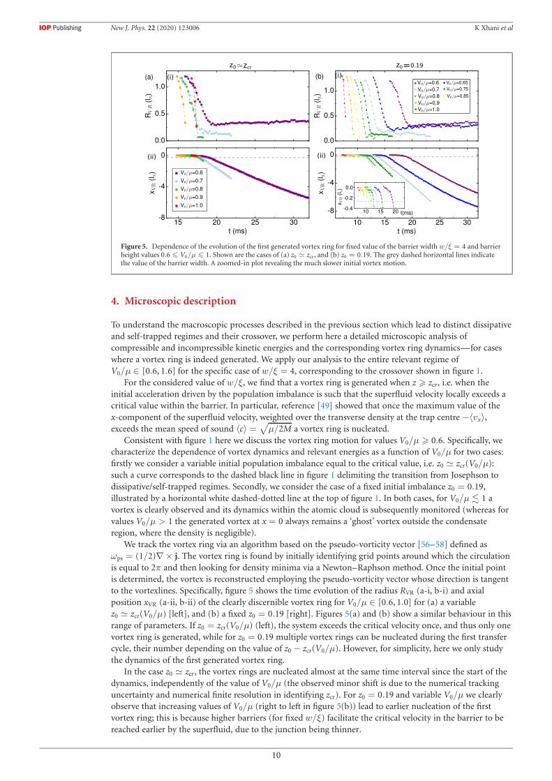
Figure 5. Dependence of the evolution of the first generated vortex ring for fixed value of the barrier width w/ξ = 4 and barrierheight values 0.6 � V0/μ � 1. Shown are the cases of (a) z0 � zcr, and (b) z0 = 0.19. The grey dashed horizontal lines indicatethe value of the barrier width. A zoomed-in plot revealing the much slower initial vortex motion.
4. Microscopic description
To understand the macroscopic processes described in the previous section which lead to distinct dissipativeand self-trapped regimes and their crossover, we perform here a detailed microscopic analysis ofcompressible and incompressible kinetic energies and the corresponding vortex ring dynamics—for caseswhere a vortex ring is indeed generated. We apply our analysis to the entire relevant regime ofV0/μ ∈ [0.6, 1.6] for the specific case of w/ξ = 4, corresponding to the crossover shown in figure 1.
For the considered value of w/ξ, we find that a vortex ring is generated when z � zcr, i.e. when theinitial acceleration driven by the population imbalance is such that the superfluid velocity locally exceeds acritical value within the barrier. In particular, reference [49] showed that once the maximum value of thex-component of the superfluid velocity, weighted over the transverse density at the trap centre −〈vx〉,exceeds the mean speed of sound 〈c〉 =
√μ/2M a vortex ring is nucleated.
Consistent with figure 1 here we discuss the vortex ring motion for values V0/μ � 0.6. Specifically, wecharacterize the dependence of vortex dynamics and relevant energies as a function of V0/μ for two cases:firstly we consider a variable initial population imbalance equal to the critical value, i.e. z0 � zcr(V0/μ):such a curve corresponds to the dashed black line in figure 1 delimiting the transition from Josephson todissipative/self-trapped regimes. Secondly, we consider the case of a fixed initial imbalance z0 = 0.19,illustrated by a horizontal white dashed-dotted line at the top of figure 1. In both cases, for V0/μ � 1 avortex is clearly observed and its dynamics within the atomic cloud is subsequently monitored (whereas forvalues V0/μ > 1 the generated vortex at x = 0 always remains a ‘ghost’ vortex outside the condensateregion, where the density is negligible).
We track the vortex ring via an algorithm based on the pseudo-vorticity vector [56–58] defined asωps = (1/2)∇× j. The vortex ring is found by initially identifying grid points around which the circulationis equal to 2π and then looking for density minima via a Newton–Raphson method. Once the initial pointis determined, the vortex is reconstructed employing the pseudo-vorticity vector whose direction is tangentto the vortexlines. Specifically, figure 5 shows the time evolution of the radius RVR (a-i, b-i) and axialposition xVR (a-ii, b-ii) of the clearly discernible vortex ring for V0/μ ∈ [0.6, 1.0] for (a) a variablez0 � zcr(V0/μ) [left], and (b) a fixed z0 = 0.19 [right]. Figures 5(a) and (b) show a similar behaviour in thisrange of parameters. If z0 = zcr(V0/μ) (left), the system exceeds the critical velocity once, and thus only onevortex ring is generated, while for z0 = 0.19 multiple vortex rings can be nucleated during the first transfercycle, their number depending on the value of z0 − zcr(V0/μ). However, for simplicity, here we only studythe dynamics of the first generated vortex ring.
In the case z0 � zcr, the vortex rings are nucleated almost at the same time interval since the start of thedynamics, independently of the value of V0/μ (the observed minor shift is due to the numerical trackinguncertainty and numerical finite resolution in identifying zcr). For z0 = 0.19 and variable V0/μ we clearlyobserve that increasing values of V0/μ (right to left in figure 5(b)) lead to earlier nucleation of the firstvortex ring; this is because higher barriers (for fixed w/ξ) facilitate the critical velocity in the barrier to bereached earlier by the superfluid, due to the junction being thinner.
10

New J. Phys. 22 (2020) 123006 K Xhani et al
In both cases, we observe that as the barrier height V0/μ decreases, the vortex ring lives longer,overcomes the barrier region and propagates further into the left well. In fact, as V0/μ decreases, thenucleated vortex ring has a larger energy (see below) hence a larger radius while propagating and a smallervelocity, as shown in figure 5. To explain this process in more detail, we note that the vortex rings arenucleated at the central plane close to x = 0 and transversally outside the local Thomas–Fermi surface.Following nucleation, and as the vortex ring moves very slowly along the negative x axis but still within thebarrier [inset to figure 5(b-ii)], each vortex ring shrinks rapidly in size in order to conserve itsincompressible kinetic energy in the presence of an increasing density due to the strong transverse densityinhomogeneity in the barrier region x ∼ 0: this is evident by the decreasing radius shown in figure 5(i),which facilitates the radius of the vortex ring to become comparable to the transversal Thomas–Fermiradius of the condensate and enter the superfluid [49]. The shrinking process of the slowly-moving vortexcontinues until the moment when the vortex ring reaches the point of maximum transversalThomas–Fermi radius (i.e. maximum condensate density), which occurs when the axial coordinate of thevortex ring, |x| ∼ 2w ∼ 0.55lx. After that, the vortex ring exits the barrier—i.e. its axial location satisfies|x(t)| � 2w—, with its radius remaining almost constant during its initial subsequent propagation; this isbecause the condensate density due to the harmonic trap does not vary much as |x| increases, until thevortex ring moves a considerable axial distance towards the trap edges. For V0/μ > 0.8, the energy of thevortex ring is insufficient to overcome the barrier and thus it shrinks within the barrier itself. Thisbehaviour is evident in figure 5 (bottom), which shows xVR remaining close to 0 (the motion of the vortexring towards negative xVR is too slow to be noticeable, except in the inset): for 0.8 < V0/μ � 1 the vortexring fails to reach x ∼ −2w, the axial location in the left well at which the transversal condensate density ismaximised. However, for sufficiently low barrier heights, the vortex rings can live for a significant amountof time: in the present context, this arises for V0/μ = 0.6 with z0 = zcr, and for V0/μ = 0.6 and 0.65 in thecase z0 = 0.19, for which the vortex ring lifetime exceeds beyond the time interval shown in figure 5. Forsuch longest-surviving vortex rings, the vortex ring propagates axially for a significant distance towards theedges of the trap, until reaching a point where its transverse spatial extent becomes comparable to the localtransverse condensate size; this results in the vortex ring increasing its size again, and eventually breakinginto two vortex lines (due to transverse inhomogeneity), as depicted in the subsequent figure 9(a).
Having identified the parameter regime of vortex ring generation, and characterised their dynamics, wenow provide information about the energy which gives insight into the observed dynamics. Building on ourearlier analysis [49], we decompose the total energy of the BEC into potential, interaction, quantum andkinetic contributions. We concentrate our attention on the kinetic energy and distinguish between thecompressible Ec
k and incompressible Eik components, respectively defined by:
Eck =
∫1
2
[(√ρv)c]2
dr and Eik =
∫1
2
[(√ρv)i]2
dr, (5)
where ∇ · (√ρv)i = 0 and ∇× (
√ρv)c = 0, with the fields (
√ρv)i and (
√ρv)c calculated via the Helmholtz
decomposition [59–62].We focus initially on the case z0 = zcr(V0/μ), and calculate the time evolution of these contributions for
different characteristic values of V0/μ ∈ [0.6, 1.6], in order to capture the entire transition from thedissipative dynamics through to the established self-trapping: our results are shown in figure 6(a).
This enables us to extract, for each V0/μ, the maximum value of Eik, whose dependence on V0/μ is
shown by the hollow points in figure 6(b). For completeness, this plot also illustrates the corresponding Eik
maxima for the fixed z0 = 0.19 case (filled points). In both cases, we clearly observe that the maximumvalues of Ei
k decrease with increasing V0/μ. The energy of the vortex ring stems from the Eik of the flow:
hence the larger Eik, the larger the available energy for the vortex ring. This effect is visible in figures 5(a-i)
and (b-i).Until now we have been concerned with the vortex nucleation and its motion, in particular whether it
can go beyond the barrier. Now we focus on the energy dissipated by the vortex and on the differencesbetween the dissipative and the pure self-trapping regime (the latter obtained for V0/μ = 1.6 and z0 = zcr
in the range of barrier heights chosen). For small values of V0/μ (V0/μ � 0.8), the vortex overcomes thebarrier and some energy of the Josephson oscillation is turned into (incompressible kinetic) energy of thevortex ring. In addition, acoustic emission takes place when the vortex, nucleated in the barrier regionoutside the condensate, enters the region of higher density [49]. For V0/μ > 0.8 the vortex shrinks andvanishes within the barrier, as illustrated in figures 5(a-i) and (b-i): its incompressible kinetic energy istransformed into compressible kinetic energy (sound waves).
To better characterize the compressible dissipation εc, we calculate the corresponding change in thecompressible kinetic energy, ΔEc
k, experienced during the nucleation and early-stage dynamics of the vortexring [49]: this time interval corresponds to the region between the two vertical dashed lines in panel
11
New J. Phys. 22 (2020) 123006 K Xhani et al
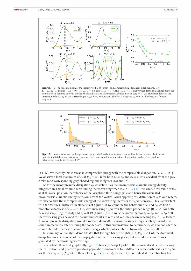
Figure 6. (a) The time evolution of the incompressible Eik (green) and compressible Ec
k (orange) kinetic energy forz0 = zcr(V0/μ) and (i) V0/μ = 0.6, (ii) V0/μ = 0.8, (iii) V0/μ = 1.17, (iv) V0/μ = 1.6. The vertical dashed black lines mark theboundaries of the time intervals during which Ec
k has a step-like increase, labelled here as ΔEck = εc. (b) The dependence of the
maximum value of Eik on the barrier height V0/μ for z0 = zcr(V0/μ) (hollow circles) and z0 = 0.19 (filled circles), for fixed
w/ξ = 4.
Figure 7. Compressible energy dissipation εc (grey circles) in the time interval bounded by the two vertical black lines infigure 6, and total energy dissipation εtot = εc + εi (orange circles) as a function of V0/μ, for fixed w/ξ = 4 and for(a) z0 = zcr(V0/μ) and (b) z0 = 0.19.
(a-i–iv). We identify this increase in compressible energy with the compressible dissipation, i.e. εc = ΔEck.
We observe a local maximum of εc at V0/μ = 0.8 for both z0 = zcr and z0 = 0.19, as evident from the greycircles (and corresponding grey-shaded region) in figures 7(a) and (b).
As for the incompressible dissipation εi, we define it as the incompressible kinetic energy densityintegrated in a small volume surrounding the vortex ring when xVR � −lx [49]. We choose this value of xVR
as at this axial position the velocity of the Josephson flow is negligible and hence the calculatedincompressible kinetic energy stems only from the vortex. When applying this definition of εi to our system,we observe that the incompressible energy of the vortex ring increases as V0/μ decreases. This is consistentwith the features illustrated in all panels of figure 5. If we combine the behaviour of εi and εc, we find amonotonic decrease of εtot = εi + εc with increasing V0/μ over the entire probed range [0.6, 1.6] for bothz0 = zcr(V0/μ) [figure 7(a)] and z0 = 0.19 [figure 7(b)]. It must be noted that for z0 = zcr and V0/μ � 0.8the vortex ring goes beyond the barrier but shrinks to zero and vanishes before reaching xVR � −lx (whereits incompressible dissipation would have been defined): its incompressible energy is totally turned intosound immediately after entering the condensate. In this circumstance, to determine εc we also consider thesecond step-like increase of compressible energy which is observable in figure 6(a-ii) at t ∼ 20 ms.
In summary, our analysis demonstrates that for high barrier heights (1 � V0/μ < 1.6), the dominantdissipation mechanism is not the propagation of the vortex ring per se, but instead the sound wavesgenerated by the vanishing vortex ring.
To illustrate this effect graphically, figure 8 shows (a) ‘carpet plots’ of the renormalised density n alongthe x-direction, and (b) corresponding population dynamics at four different characteristic values of V0/μ
for the case z0 = zcr(V0/μ). In these plots figures 8(i)–(iv), the density n is evaluated by subtracting from
12
New J. Phys. 22 (2020) 123006 K Xhani et al
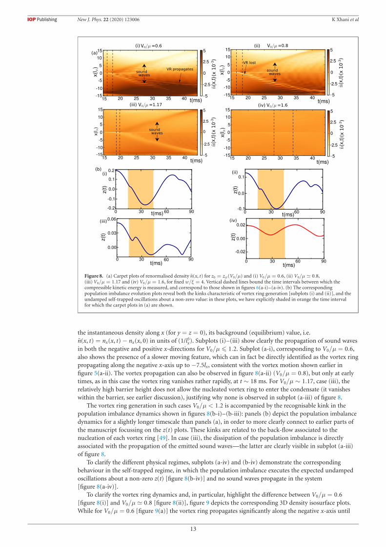
Figure 8. (a) Carpet plots of renormalised density n(x, t) for z0 = zcr(V0/μ) and (i) V0/μ = 0.6, (ii) V0/μ � 0.8,(iii) V0/μ = 1.17 and (iv) V0/μ = 1.6, for fixed w/ξ = 4. Vertical dashed lines bound the time intervals between which thecompressible kinetic energy is measured, and correspond to those shown in figures 6(a-i)–(a-iv). (b) The correspondingpopulation imbalance evolution plots reveal both the kinks characteristic of vortex ring generation [subplots (i) and (ii)], and theundamped self-trapped oscillations about a non-zero value: in these plots, we have explicitly shaded in orange the time intervalfor which the carpet plots in (a) are shown.
the instantaneous density along x (for y = z = 0), its background (equilibrium) value, i.e.n(x, t) = nx(x, t) − nx(x, 0) in units of (1/l3x). Subplots (i)–(iii) show clearly the propagation of sound wavesin both the negative and positive x-directions for V0/μ � 1.2. Subplot (a-i), corresponding to V0/μ = 0.6,also shows the presence of a slower moving feature, which can in fact be directly identified as the vortex ringpropagating along the negative x-axis up to −7.5lx, consistent with the vortex motion shown earlier infigure 5(a-ii). The vortex propagation can also be observed in figure 8(a-ii) (V0/μ = 0.8), but only at earlytimes, as in this case the vortex ring vanishes rather rapidly, at t ∼ 18 ms. For V0/μ ∼ 1.17, case (iii), therelatively high barrier height does not allow the nucleated vortex ring to enter the condensate (it vanisheswithin the barrier, see earlier discussion), justifying why none is observed in subplot (a-iii) of figure 8.
The vortex ring generation in such cases V0/μ < 1.2 is accompanied by the recognisable kink in thepopulation imbalance dynamics shown in figures 8(b-i)–(b-iii): panels (b) depict the population imbalancedynamics for a slightly longer timescale than panels (a), in order to more clearly connect to earlier parts ofthe manuscript focussing on the z(t) plots. These kinks are related to the back-flow associated to thenucleation of each vortex ring [49]. In case (iii), the dissipation of the population imbalance is directlyassociated with the propagation of the emitted sound waves—the latter are clearly visible in subplot (a-iii)of figure 8.
To clarify the different physical regimes, subplots (a-iv) and (b-iv) demonstrate the correspondingbehaviour in the self-trapped regime, in which the population imbalance executes the expected undampedoscillations about a non-zero z(t) [figure 8(b-iv)] and no sound waves propagate in the system[figure 8(a-iv)].
To clarify the vortex ring dynamics and, in particular, highlight the difference between V0/μ = 0.6[figure 8(i)] and V0/μ � 0.8 [figure 8(ii)], figure 9 depicts the corresponding 3D density isosurface plots.While for V0/μ = 0.6 [figure 9(a)] the vortex ring propagates significantly along the negative x-axis until
13

New J. Phys. 22 (2020) 123006 K Xhani et al
Figure 9. Snapshots of the 3D isosurface density plots depicting the vortex ring generation and evolution for (a) V0/μ = 0.6and (b) V0/μ � 0.8, taken at z0 = zcr(V0/μ) and w/ξ = 4. Note the different evolution times in the two cases.
xVR ∼ −8lx, eventually breaking into two vortex lines when it reaches the boundary, for the slightly higherV0/μ � 0.8 the vortex ring shrinks and vanishes before reaching xVR ∼ −1lx.
These results complete our study of the microscopic differences between the dissipative regime for0.8 � V0/μ � 1.17 and the pure self-trapped regime at V0/μ ∼ 1.6.
We have given a detailed phase diagram for the parameter regime when different dynamical behaviourscan be expected, and characterised our findings in terms of energetic considerations and vortexgeneration/dynamics—in the context of an elongated 3D condensate corresponding to, and motivated by,the LENS experimental geometry [15, 16]. Our study would not be complete without a demonstration thatour findings qualitatively hold across different experimentally-relevant geometries.
5. Phase diagram extension to an isotropic trap
In this section we show the broad relevance of our previously characterized phase diagram regimes byperforming the same analysis in the context of an isotropic (spherical) trap. To make a connection with thefeatures already studied earlier, we keep the condensate number fixed to 60 000, and all three harmonic trapfrequencies are fixed to the previously used ωx = 2π × 15 Hz. We thus set ωy = ωz = ωx = 2π × 15 Hzwhich (for N = 60 000) gives μ � 17�ωx and ξ � 1.3 μm � 0.17lx. This parameter choice—which iswithin experimental reach—has been made as it significantly increases the values of the populationimbalance for which interesting dynamical crossovers can be observed by about an order of magnitudecompared to the small values encountered in the elongated geometry—thus making the observation of ourfindings highly experimentally relevant.
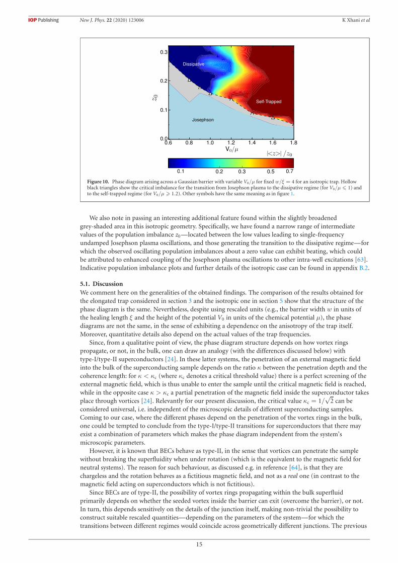
A plot revealing the emergence of the different dynamical regimes for variable z0 as a function ofV0/μ ∈ [0.6, 1.8] (similar to that of figure 1) is shown in figure 10. The important main conclusion arisingfrom this figure is that—despite huge differences in the values of zcr in relation to the elongated phasediagram of figure 1—qualitatively we recover the same picture. Values of z0 below some threshold exhibitJosephson plasma sinusoidal oscillations about a zero value. For values z0 � zcr one instead transitions toeither a dissipative regime (V0/μ � 1.0), or a self-trapped regime (V0/μ � 1.2), with a crossover occuringat intermediate values of V0/μ. In particular, for 0.6 � V0/μ � 1, the vortex ring enters the localThomas–Fermi surface and propagates axially into the left well, with a lifetime which decreases withincreasing barrier height, as found for the elongated trap.
The transition to the self-trapped regime is found to occur for V0/μ � 1.2, i.e. at a slightly smaller valueof V0/μ with respect to the elongated trap (where it emerged around V0/μ = 1.6 for the same w/ξ = 4).Importantly, we observe that the critical imbalances for the spherical trap are higher with respect to thosepreviously found in the elongated trap due to the increase of the ratio of the tunnelling to self-interactionenergy.
14
New J. Phys. 22 (2020) 123006 K Xhani et al
Figure 10. Phase diagram arising across a Gaussian barrier with variable V0/μ for fixed w/ξ = 4 for an isotropic trap. Hollowblack triangles show the critical imbalance for the transition from Josephson plasma to the dissipative regime (for V0/μ � 1) andto the self-trapped regime (for V0/μ � 1.2). Other symbols have the same meaning as in figure 1.
We also note in passing an interesting additional feature found within the slightly broadenedgrey-shaded area in this isotropic geometry. Specifically, we have found a narrow range of intermediatevalues of the population imbalance z0 —located between the low values leading to single-frequencyundamped Josephson plasma oscillations, and those generating the transition to the dissipative regime—forwhich the observed oscillating population imbalances about a zero value can exhibit beating, which couldbe attributed to enhanced coupling of the Josephson plasma oscillations to other intra-well excitations [63].Indicative population imbalance plots and further details of the isotropic case can be found in appendix B.2.
5.1. DiscussionWe comment here on the generalities of the obtained findings. The comparison of the results obtained forthe elongated trap considered in section 3 and the isotropic one in section 5 show that the structure of thephase diagram is the same. Nevertheless, despite using rescaled units (e.g., the barrier width w in units ofthe healing length ξ and the height of the potential V0 in units of the chemical potential μ), the phasediagrams are not the same, in the sense of exhibiting a dependence on the anisotropy of the trap itself.Moreover, quantitative details also depend on the actual values of the trap frequencies.
Since, from a qualitative point of view, the phase diagram structure depends on how vortex ringspropagate, or not, in the bulk, one can draw an analogy (with the differences discussed below) withtype-I/type-II superconductors [24]. In these latter systems, the penetration of an external magnetic fieldinto the bulk of the superconducting sample depends on the ratio κ between the penetration depth and thecoherence length: for κ < κc (where κc denotes a critical threshold value) there is a perfect screening of theexternal magnetic field, which is thus unable to enter the sample until the critical magnetic field is reached,while in the opposite case κ > κc a partial penetration of the magnetic field inside the superconductor takesplace through vortices [24]. Relevantly for our present discussion, the critical value κc = 1/
√2 can be
considered universal, i.e. independent of the microscopic details of different superconducting samples.Coming to our case, where the different phases depend on the penetration of the vortex rings in the bulk,one could be tempted to conclude from the type-I/type-II transitions for superconductors that there mayexist a combination of parameters which makes the phase diagram independent from the system’smicroscopic parameters.
However, it is known that BECs behave as type-II, in the sense that vortices can penetrate the samplewithout breaking the superfluidity when under rotation (which is the equivalent to the magnetic field forneutral systems). The reason for such behaviour, as discussed e.g. in reference [64], is that they arechargeless and the rotation behaves as a fictitious magnetic field, and not as a real one (in contrast to themagnetic field acting on superconductors which is not fictitious).
Since BECs are of type-II, the possibility of vortex rings propagating within the bulk superfluidprimarily depends on whether the seeded vortex inside the barrier can exit (overcome the barrier), or not.In turn, this depends sensitively on the details of the junction itself, making non-trivial the possibility toconstruct suitable rescaled quantities—depending on the parameters of the system—for which thetransitions between different regimes would coincide across geometrically different junctions. The previous
15

New J. Phys. 22 (2020) 123006 K Xhani et al
argument demonstrates the challenges in identifying appropriate dimensionless quantities, but does notshow that one cannot in principle construct such suitable rescaled quantities. This is an important issuebeyond the scope of this work, which certainly deserves further study.
6. Conclusions
We have characterised the full phase diagram describing the dynamical regimes that can emerge across aJosephson junction created by a Gaussian barrier: Josephson plasma, self-trapping, and dissipative. Ouranalysis bridges the gap between numerous previous studies depicting either a transition from Josephsonplasma to macroscopic quantum self-trapping, or Josephson plasma to dissipative regimes. As expected, wehave found the existence of undamped symmetric Josephson plasma oscillations for population imbalancesbelow their corresponding critical values. Increasing the initial population imbalance across the barrierleads to a transition to a different regime, which depends on a specific combination of barrier height andwidth. Specifically, for relatively large barrier heights/widths, the system transitions to a self-trapped state.Once the population imbalance exceeds a critical value, it exhibits the established macroscopic quantumself-trapping regime, which features regular symmetric oscillations about a non-zero value, and a runningrelative phase, whereas increasing the initial population imbalance much beyond that value leads to morecomplicated self-trapped states with oscillations at multiple frequencies. In the other extreme of smallbarrier widths/heights, the system transitions—with increasing z0 —to a dissipative regime, which sees theemission of acoustic (sound) energy and the generation and propagation of vortex rings, a distinctivefeature associated with phase-slips known in other physical systems with Josephson junctions, and leadingto the resistive superflow. The critical value of z0 in which dissipative behaviour is observed is always largerthan the corresponding one when the system transitions (for a higher/broader barrier) to the self-trappedregime.
Our work shows that for elongated traps such as the ones studied in [15, 16], where only the transitionfrom the Josephson plasma regime to the dissipative one was observed, the self-trapping regime can in factalso be observed for higher and wider barriers, thus making concrete predictions which can beexperimentally tested.
As a counterpart, our result indicates that for traps in which only the transition from the Josephsonplasma to the self-trapped regime has been seen (such as [8], which had an aspect ratio ∼ 1), the dissipativeregime can also be observed by lowering the barrier height (to values slightly below, but still a sizeablefraction of, μ).
So our work suggests that for any geometry we can find all three dynamical regimes, and that suchregimes should be experimentally observable within a single experimental set-up by careful control of thebarrier height or width.
Interestingly we also find—beyond a smooth, and rather irregular, crossover between dissipative andself-trapped regimes—that spherical traps have another regime that should be observable in currentexperiments, in which the coupling of the Josephson plasma frequency and other collective modes becomerelevant [63] and can lead to a beating. The latter becomes particularly noticeable as the system begins totransition from the pure single-frequency Josephson to the dissipative regimes. This feature appears to bemore pronounced in spherical geometries, rather than elongated ones. The spherical geometry also leads tothe emergence of such features, and other crossover behaviours, at higher population imbalances, whichshould make such features easier to investigate experimentally.
Our results also clarify what distinguishes between the dissipative and macroscopic quantumself-trapping regimes, not just in terms of z(t) and φ(t), but also in terms of vortex ring dynamics. As V0/μ
increases, the vortex rings go from a regime in which they can propagate (leaving the barrier region), to aregime where they shrink within the barrier. Whether the vortex ring leaves or not the barrier is defined bythe value of incompressible kinetic energy that is present in the system. In the crossover between theself-trapped and dissipative regimes, the main difference comes from sound waves: specifically, in theself-trapped regime (for z0 values slightly larger than zcr) there are practically no sound waves, while in thedissipative regime such sound waves propagate and make the condensate dissipate.
After two decades of cold atom experiments studying weak links, the unified description given in thepresent paper allows to merge different previous experimental observations together. Our work is alsorelevant for studying dissipation in a fermionic superfluid controllably tuned across the BEC–BCScrossover, which will form the basis of future work.
Finally, we observe that the results we presented are applicable to ultracold Josephson junctions forwhich the mean field Gross–Pitaevskii description holds. In view of experimental realizations of weak linksbetween low-dimensional ultracold atoms, it would be very interesting to study how the dynamical phasediagram presented here is modified by the quantum fluctuations present in such systems. In the future we
16

New J. Phys. 22 (2020) 123006 K Xhani et al
therefore plan to extend our study in 2D to highlight the role of dimensionality and thermal fluctuations in2D ultracold Josephson junctions.
Data supporting this publication is openly available under an Open Data Commons Open DatabaseLicense [69].
Acknowledgments
We thank Tilman Enss, Francesco Scazza, Augusto Smerzi and Matteo Zaccanti for useful discussions. Thiswork was supported by the QuantERA project NAQUAS (EPSRC EP/R043434/1), EPSRC projectEP/R005192/1 and the European Research Council under GA No. 307032 QuFerm2D, the Italian MIURunder the PRIN2017 project CEnTraL.
Appendix A. Comparison to two-model predictions
In the standard two-mode model [30, 32, 65] the wavefunction can be expressed as a linear superposition ofthe left and right condensate wave functions, i.e.
ψ(r, t) = ψL(t) · ηL(r) + ψR(t) · ηR(r), (A.1)
where ψL(t) =√
NL eiφL and ψR(t) =√
NR eiφR and∫ηi · ηj dr = δi,j, with i, j = left, right with NL(R) and
φL(R) the number of particles and the condensate phase in the left and right well respectively. The left andright wavefunctions can be found from the spatially symmetric and the first antisymmetric statewavefunctions as ηR,L = (η+ ± η−)/
√2. The symmetric state is the ground state corresponding to zero
initial imbalance and zero initial relative phase, while the antisymmetric state instead has a correspondingrelative phase of π. An atomic Josephson junction is described in terms of the on-site interaction energy Uand the tunnelling energy K, from which we can extract the critical imbalance by using the formula
zcr �√
8KUN . The tunnelling energy is estimated from the difference between the antisymmetric and the
symmetric state energy 2K � EJ = (E− − E+) = ΔE and thus zcr �√
4ΔEUN . The onsite interaction energy
instead can be found from the linear two-mode model Ulin = g∫η4
L dr or from the nonlinear two-modemodel [65] as UNL = 2(∂μ/∂N).
We use GPE simulations in order to find the symmetric and antisymmetric states for a linear tiltedpotential ε = 0, and from those we extract the tunnelling energy. The extracted values of the zcr from thetwo-mode model are shown in figure A1(a-i) for fixed barrier width w/ξ = 4 and barrier heights0.6 � V0/μ � 2.1 while figure A1(b-i) shows the corresponding results for V0/μ = 1.17 and a variablebarrier width 4 � w/ξ � 10. We note that the critical imbalance from the two-mode model sets thetransition to the self-trapped regime which in our case happens at fixed w/ξ = 4 and V0/μ � 1.6, and forw/ξ � 7 for fixed V0/μ = 1.17. We also show in these subplots the corresponding extracted values of zcr
from the GPE simulations finding good agreement for V0/μ � 1.2 and for all the explored barrier widths inthe case of fixed V0/μ = 1.17.
The GPE prediction of zcr is found by solving again the GPE numerically, but this time with an initiallinear potential −εx along the x direction, thus leading to values z0 = 0. The critical imbalance is definedthen by looking at the time evolution of z(t). In the regime of the Josephson plasma oscillation and forEJ � Ec the two-mode model prediction for the oscillation frequency is:
ωJ �√
EJEc
�=
√ΔEUlin (NL)N
�, (A.2)
whose behaviour is shown in the right subplots of figure A1 ((a-ii), (b-ii)). Specifically, we plot ωJ/ωx as afunction of V0/μ at fixed w/ξ = 4 [(a-ii)] and as a function of w/ξ at fixed V0/μ [figure A1(b-ii)], showingboth two-mode model predictions, and corresponding numerical GPE results. Together with the extractedvalues from the GPE simulations. The two-mode model predicts the Josephson plasma frequency well forV0/μ � 1.6 in the case of fixed w/ξ = 4 and for w/ξ � 7 for fixed V0/μ = 1.17.
Appendix B. Further characterization of dynamical regimes crossover
The main text has focussed on the identification of the 3 key dynamical regimes of interest, namelyJosephson plasma oscillations, dissipative regime, and self-trapped regime. As discussed, a convenient wayto characterize such regimes is by means of the distinct dynamical population imbalance curves, z(t), which
17

New J. Phys. 22 (2020) 123006 K Xhani et al
Figure A1. Critical initial population imbalance (left column, (i)) and corresponding Josephson plasma frequency (rightcolumn, (ii)) for the elongated trap, as a function of (a) barrier height V0/μ at fixed w/ξ = 4, or (b) w/ξ at fixed V0/μ = 1.17.All subplots show results extracted from GPE simulations (blue squares, triangles), and from the linear (orange circles) andnonlinear (violet circles) two-mode model. The Josephson plasma frequencies are extracted from the GPE simulations by fittingwith a sinusoidal function z(t) for z0 < zcr. Vertical dashed line in (a) indicates the specific barrier height V0/μ = 1.17 used in(b). The data are for ωx = 2π × 15 Hz, ωy = 2π × 187.5 Hz, ωz = 2π × 148 Hz, and a particle number N = 60 000.
reveal a plethora of relevant informations. In this appendix we discuss in more detail intricate details aboutthe system behaviour and the transitions and crossovers between the identified regimes in an elongated, andan isotropic, harmonic trap.
B.1. Elongated trapInitially, we focus on the elongated trap (LENS experimental geometry [13, 16]). We study how z(t) changesby varying the barrier parameters (height or width) at fixed initial population imbalance z0 [appendixB.1.1], and then present further details of its behaviour in the crossover regimes [appendix B.1.2].
B.1.1. Variable barrier height/width
The evolution of z(t) at fixed initial population imbalance z0 as the system transitions from Josephsonplasma to dissipative and then to self-trapped regimes is shown in figure B1 by increasing either (a) V0/μ atfixed w/ξ = 4, or (b) w/ξ at fixed V0/μ = 1.17. This corresponds to horizontally traversing the phasediagram of, respectively, figures 1 and 3. In both plots we see a clear transition from Josephson plasmaoscillations (blue lines), to a dissipative regime (purple lines), followed by a rather complicated transition toa self-trapped state. Due to the previously identified dependence of zcr on V0/μ (largely related to theprofile of the maximum current versus V0/μ found by considering first and second order terms in thetunnelling Hamiltonian [49]), a simple inspection of the phase diagram of figures 1 and 3 reveals that suchhorizontal cuts through the phase diagrams imply that the system will enter the self-trapped regime with avalue of z0 � zcr, such that we do not expect to observe the emergence of the pure two-mode regime, butrather the multi-frequency self-trapped state analysed below. Thus, these two subplots reveal thecomplicated intermediate region for large z0 > zcr when the system transitions from the dissipative to theself-trapped regime, i.e. the transition from the blue to the red regions in figures 1 and 3 respectively.
B.1.2. Further dynamical regime details in an elongated trap
Next, we present a systematic characterization of the different evolution of z(t) across the different regimes,in order to clearly highlight the nature of the different observed crossovers. In particular, figure B2 showsthe complex dependence of the evolution of z(t) for different values of the parameters z0/zcr and V0/μ (andbarriers with w/ξ = 4), as clearly identified in the individual subplots. This figure is organised across fourrows, with the ratio of z0/zcr increasing from bottom to top from values <1 to values >1, and four columns
18
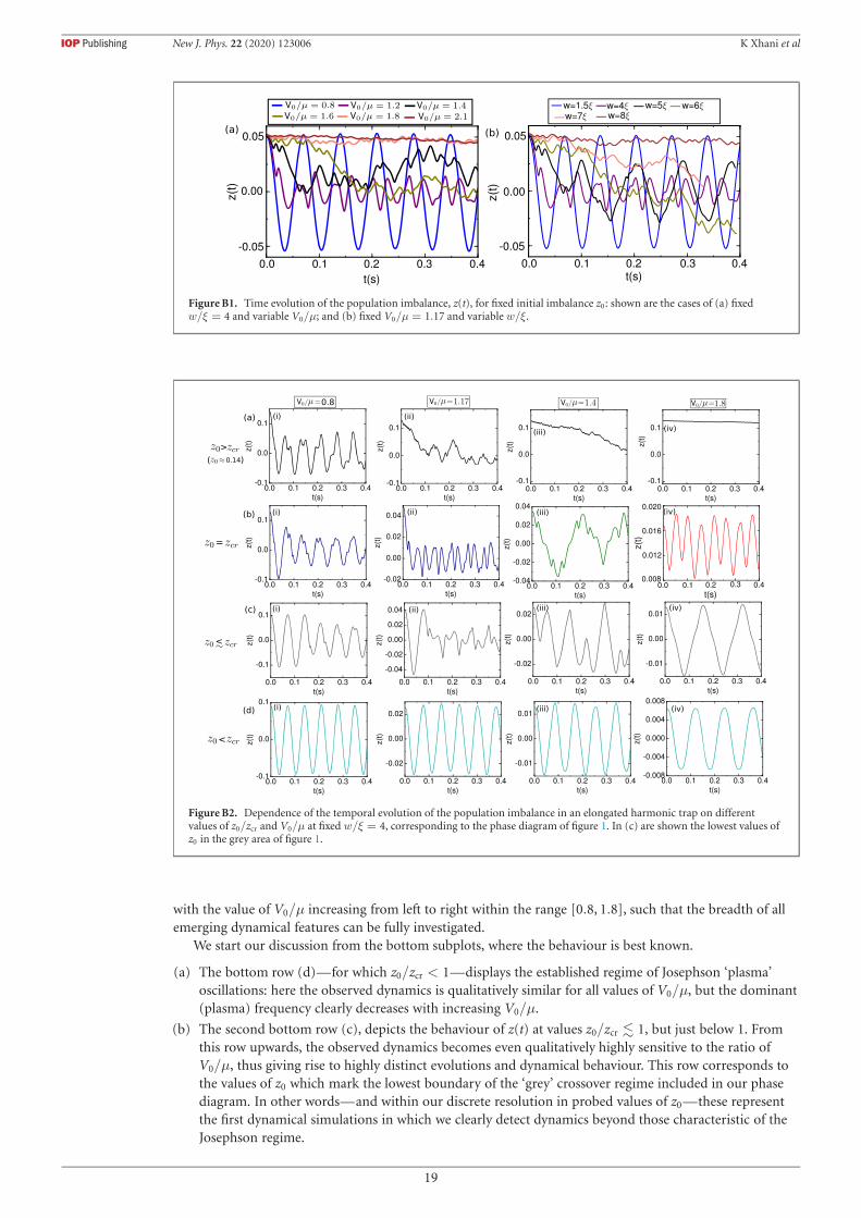
New J. Phys. 22 (2020) 123006 K Xhani et al
Figure B1. Time evolution of the population imbalance, z(t), for fixed initial imbalance z0: shown are the cases of (a) fixedw/ξ = 4 and variable V0/μ; and (b) fixed V0/μ = 1.17 and variable w/ξ.
Figure B2. Dependence of the temporal evolution of the population imbalance in an elongated harmonic trap on differentvalues of z0/zcr and V0/μ at fixed w/ξ = 4, corresponding to the phase diagram of figure 1. In (c) are shown the lowest values ofz0 in the grey area of figure 1.
with the value of V0/μ increasing from left to right within the range [0.8, 1.8], such that the breadth of allemerging dynamical features can be fully investigated.
We start our discussion from the bottom subplots, where the behaviour is best known.
(a) The bottom row (d)—for which z0/zcr < 1—displays the established regime of Josephson ‘plasma’oscillations: here the observed dynamics is qualitatively similar for all values of V0/μ, but the dominant(plasma) frequency clearly decreases with increasing V0/μ.
(b) The second bottom row (c), depicts the behaviour of z(t) at values z0/zcr � 1, but just below 1. Fromthis row upwards, the observed dynamics becomes even qualitatively highly sensitive to the ratio ofV0/μ, thus giving rise to highly distinct evolutions and dynamical behaviour. This row corresponds tothe values of z0 which mark the lowest boundary of the ‘grey’ crossover regime included in our phasediagram. In other words—and within our discrete resolution in probed values of z0 —these representthe first dynamical simulations in which we clearly detect dynamics beyond those characteristic of theJosephson regime.
19

New J. Phys. 22 (2020) 123006 K Xhani et al
Starting from the left, the case V0/μ = 0.8 [(c-i)] presents dissipative dynamical behaviour, butthere is no early kink in z(t) [i.e. during the first population transfer cycle] which is characteristic ofvortex ring generation: such kinks do appear in later oscillation cycles and eventually lead to thedecaying oscillatory dynamics. As V0/μ increases the behaviour becomes more complicated, indicatinga gradual transition from dissipative to anharmonic oscillations about a zero mean value for highervalues of V0/μ = 1.8 [(c-iv)]—the latter regime has been previously discussed in the literature in thecontext of the emergence of MQST.
(c) The second top row (b) corresponds to the critical case z0/zcr = 1. This corresponds precisely to thecritical population imbalance limit highlighted in our phase diagram. This row thus maps out theupper end of the grey area of the phase diagram, defining the critical line which identifies the transitionto the distinct dynamical regime characterized by the colour of |〈z(t)〉|/z0. The leftmost casecorresponding to V0/μ = 0.8 [(b-i)] has been previously discussed [see figures 1 and 2 of main paper]and corresponds to the characteristic case of an early clear vortex ring generation during the firstpopulation transfer cycle. Increasing V0/μ to 1.17 [(b-ii)]—which corresponds precisely to the casediscussed in figures 8(a-iii) and (b-iii)—demonstrates a rapid decay of the population oscillationsaccompanied by significant sound emission, and a multi-frequency oscillation about a zero mean value,thus signalling the end of the dissipative regime. Further increase of V0/μ to 1.4[(b-iii)]—corresponding to what we have labelled as ‘intermediate’ regime between dissipative andself-trapped limits—leads to complicated oscillations still crossing the z = 0 boundary, but indicating agradual transition towards the self-trapped regime, in which z(t) can still exhibit multi-modeoscillations, but now about a non-zero mean value [(b-iv)].
(d) The top row (a) corresponds to a case of (approximately) constant initial population imbalancez0 ≈ 0.14, chosen such that it is above all corresponding critical values zcr(V0/μ) in all casesconsidered. For low V0/μ = 0.8 [(a-i)], we see the consecutive generation of multiple vortex rings, anda very rapid transition to complicated multi-mode oscillations about a zero mean value. IncreasingV0/μ further to 1.17 [(a-ii)] leads to a decaying pattern approaching zero with some residual irregularoscillations. The further increase to V0/μ = 1.4 [(a-iii)] indicates a gradual transition towards anunstable self-trapped state, with such a case still exhibiting an intermediate value of |〈z(t)〉|/z0 which isclearly distinct from both limiting values of 0 (dissipative) and 1 (fully self-trapped). Due to the curvednature of the critical population imbalance line marking the phase diagram of figure 1, we recall thatthe value of zcr is reduced with increasing V0/μ. As a result, when traversing the phase diagramapproximately horizontally (i.e. for a near constant value of z0), we are bound to end up in a highlyexcited multi-frequency self-trapped state, for which |〈z(t)〉|/z0 ∼ 1, as found here for V0/μ = 1.8[(a-iv)].
It is also instructive to inspect figure B2 vertically, i.e. across a single column, from bottom to top. Forlow values of V0/μ = 0.8, increasing z0 leads to a clear transition from Josephson [(d-i)] to single- [(b-i)],and multi-vortex [(a-i)] dissipative dynamics, mediated by dissipative dynamics in the grey region [(c-i)],which however do not exhibit a vortex ring during the first population transfer cycle.
In the other limiting case of high V0/μ = 1.8, the harmonic Josephson oscillations [(d-iv)] give way toanharmonic oscillations about a zero mean value [(c-iv)] (corresponding to the bottom of the ‘grey’region), before shifting to periodic oscillations about a non-zero mean value [(b-iv)] and, for valuesz0 � zcr(V0/μ), to irregular multi-frequency self-trapped states, with |〈z(t)〉|/z0 ∼ 1.
The in-between regimes V0/μ = 1.17 (ii) and 1.4 (iii) display with increasing z0 a more gradualevolution to regimes which for z0 > zcr(V0/μ) lie in the ‘intermediate’ regime between dissipative andself-trapped.
This practically concludes our analysis of the dependence of the evolution of z(t) on both z0/zcr andV0/μ (done here for fixed w/ξ), further supporting our discussion of the obtained phase diagrams for theelongated case found in the main text.
In this complicated nonlinear system, there are two further interesting features we wish to highlight:Firstly, we touch briefly upon the characterization of the regime we have more broadly termed ‘pure
self-trapped’ in this work. Pure self-trapped here refers to a well-defined regime in which there are periodicwell-defined oscillations in the population imbalance with frequency νMQST = Δμ/h (where Δμ is thechemical potential difference between the two-condensates), whose sign however does not change, withassociated running phase. Such self-trapping emerges in its purest form for values of z0 equal to, ormarginally above, zcr, and for values V0/μ sufficiently exceeding 1 for the given barrier width [30, 32]. Thisand the behaviour for higher z0 > zcr (as shown in (a-iv)) is discussed further in appendix B.1.3 below.
Moreover, the Josephson regime in ultracold atoms is typically associated with a single dominantfrequency, the plasma frequency, determined by the two-mode model. However, the two-mode
20
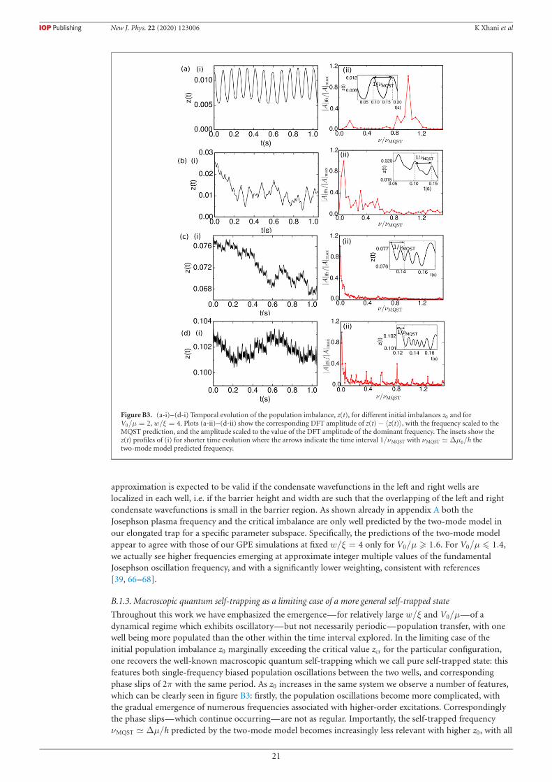
New J. Phys. 22 (2020) 123006 K Xhani et al
Figure B3. (a-i)–(d-i) Temporal evolution of the population imbalance, z(t), for different initial imbalances z0 and forV0/μ = 2, w/ξ = 4. Plots (a-ii)–(d-ii) show the corresponding DFT amplitude of z(t) − 〈z(t)〉, with the frequency scaled to theMQST prediction, and the amplitude scaled to the value of the DFT amplitude of the dominant frequency. The insets show thez(t) profiles of (i) for shorter time evolution where the arrows indicate the time interval 1/νMQST with νMQST � Δμ0/h thetwo-mode model predicted frequency.
approximation is expected to be valid if the condensate wavefunctions in the left and right wells arelocalized in each well, i.e. if the barrier height and width are such that the overlapping of the left and rightcondensate wavefunctions is small in the barrier region. As shown already in appendix A both theJosephson plasma frequency and the critical imbalance are only well predicted by the two-mode model inour elongated trap for a specific parameter subspace. Specifically, the predictions of the two-mode modelappear to agree with those of our GPE simulations at fixed w/ξ = 4 only for V0/μ � 1.6. For V0/μ � 1.4,we actually see higher frequencies emerging at approximate integer multiple values of the fundamentalJosephson oscillation frequency, and with a significantly lower weighting, consistent with references[39, 66–68].
B.1.3. Macroscopic quantum self-trapping as a limiting case of a more general self-trapped state
Throughout this work we have emphasized the emergence—for relatively large w/ξ and V0/μ—of adynamical regime which exhibits oscillatory—but not necessarily periodic—population transfer, with onewell being more populated than the other within the time interval explored. In the limiting case of theinitial population imbalance z0 marginally exceeding the critical value zcr for the particular configuration,one recovers the well-known macroscopic quantum self-trapping which we call pure self-trapped state: thisfeatures both single-frequency biased population oscillations between the two wells, and correspondingphase slips of 2π with the same period. As z0 increases in the same system we observe a number of features,which can be clearly seen in figure B3: firstly, the population oscillations become more complicated, withthe gradual emergence of numerous frequencies associated with higher-order excitations. Correspondinglythe phase slips—which continue occurring—are not as regular. Importantly, the self-trapped frequencyνMQST � Δμ/h predicted by the two-mode model becomes increasingly less relevant with higher z0, with all
21
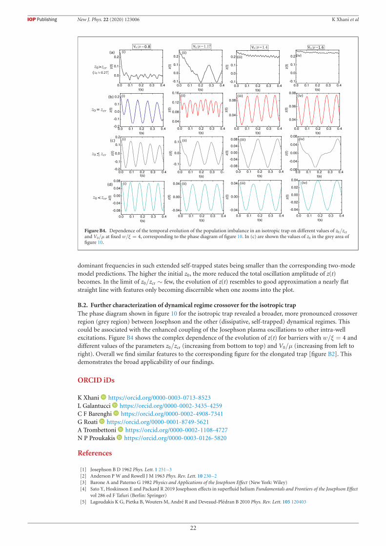
New J. Phys. 22 (2020) 123006 K Xhani et al
Figure B4. Dependence of the temporal evolution of the population imbalance in an isotropic trap on different values of z0/zcr
and V0/μ at fixed w/ξ = 4, corresponding to the phase diagram of figure 10. In (c) are shown the values of z0 in the grey area offigure 10.
dominant frequencies in such extended self-trapped states being smaller than the corresponding two-modemodel predictions. The higher the initial z0, the more reduced the total oscillation amplitude of z(t)becomes. In the limit of z0/zcr ∼ few, the evolution of z(t) resembles to good approximation a nearly flatstraight line with features only becoming discernible when one zooms into the plot.
B.2. Further characterization of dynamical regime crossover for the isotropic trapThe phase diagram shown in figure 10 for the isotropic trap revealed a broader, more pronounced crossoverregion (grey region) between Josephson and the other (dissipative, self-trapped) dynamical regimes. Thiscould be associated with the enhanced coupling of the Josephson plasma oscillations to other intra-wellexcitations. Figure B4 shows the complex dependence of the evolution of z(t) for barriers with w/ξ = 4 anddifferent values of the parameters z0/zcr (increasing from bottom to top) and V0/μ (increasing from left toright). Overall we find similar features to the corresponding figure for the elongated trap [figure B2]. Thisdemonstrates the broad applicability of our findings.
ORCID iDs
K Xhani https://orcid.org/0000-0003-0713-8523L Galantucci https://orcid.org/0000-0002-3435-4259C F Barenghi https://orcid.org/0000-0002-4908-7341G Roati https://orcid.org/0000-0001-8749-5621A Trombettoni https://orcid.org/0000-0002-1108-4727N P Proukakis https://orcid.org/0000-0003-0126-5820
References
[1] Josephson B D 1962 Phys. Lett. 1 251–3[2] Anderson P W and Rowell J M 1963 Phys. Rev. Lett. 10 230–2[3] Barone A and Paterno G 1982 Physics and Applications of the Josephson Effect (New York: Wiley)[4] Sato Y, Hoskinson E and Packard R 2019 Josephson effects in superfluid helium Fundamentals and Frontiers of the Josephson Effect
vol 286 ed F Tafuri (Berlin: Springer)[5] Lagoudakis K G, Pietka B, Wouters M, Andre R and Deveaud-Pledran B 2010 Phys. Rev. Lett. 105 120403
22
New J. Phys. 22 (2020) 123006 K Xhani et al
[6] Adiyatullin A F, Anderson M D, Flayac H, Portella-Oberli M T, Jabeen F, Ouellet-Plamondon C, Sallen G C and Deveaud B 2017Nat. Commun. 8 1329
[7] Cataliotti F S, Burger S, Fort C, Maddaloni P, Minardi F, Trombettoni A, Smerzi A and Inguscio M 2001 Science 293 843–6[8] Albiez M, Gati R, Fölling J, Hunsmann S, Cristiani M and Oberthaler M K 2005 Phys. Rev. Lett. 95 010402[9] Anker T, Albiez M, Gati R, Hunsmann S, Eiermann B, Trombettoni A and Oberthaler M K 2005 Phys. Rev. Lett. 94 020403
[10] Schumm T, Hofferberth S, Andersson L M, Wildermuth S, Groth S, Bar-Joseph I, Schmiedmayer J and Krüger P 2005 Nat. Phys. 157–62
[11] Shin Y, Saba M, Pasquini T A, Ketterle W, Pritchard D E and Leanhardt A E 2004 Phys. Rev. Lett. 92 050405[12] Levy S, Lahoud E, Shomroni I and Steinhauer J 2007 Nature 449 579–83[13] Spagnolli G et al 2017 Phys. Rev. Lett. 118 230403[14] LeBlanc L J, Bardon A B, McKeever J, Extavour M H T, Jervis D, Thywissen J H, Piazza F and Smerzi A 2011 Phys. Rev. Lett. 106
025302[15] Valtolina G et al 2015 Science 350 1505–8[16] Burchianti A, Scazza F, Amico A, Valtolina G, Seman J A, Fort C, Zaccanti M, Inguscio M and Roati G 2018 Phys. Rev. Lett. 120
025302[17] Kwon W J, Del Pace G, Panza R, Inguscio M, Zwerger W, Zaccanti M, Scazza F and Roati G 2020 Science 369 84–8[18] Luick N, Sobirey L, Bohlen M, Singh V P, Mathey L, Lompe T and Moritz H 2020 Science 369 89–91[19] Pace G D, Kwon W J, Zaccanti M, Roati G and Scazza F 2020 arXiv:2010.00582[20] Williams J, Walser R, Cooper J, Cornell E and Holland M 1999 Phys. Rev. A 59 R31–4[21] Smerzi A, Trombettoni A, Lopez-Arias T, Fort C, Maddaloni P, Minardi F and Inguscio M 2003 Eur. Phys. J. B 31 457–61[22] Gross C, Zibold T, Nicklas E, Esteve J and Oberthaler M K 2010 Nature 464 1165–9[23] Riedel M F, Böhi P, Li Y, Hansch T W, Sinatra A and Treutlein P 2010 Nature 464 1170–3[24] Tinkham M 1996 Introduction to Superconductivity 2nd edn (New York: McGraw-Hill)[25] Edwards M 2013 Nat. Phys. 9 68–9[26] Ryu C, Blackburn P W, Blinova A A and Boshier M G 2013 Phys. Rev. Lett. 111 205301[27] Ryu C, Samson E C and Boshier M G 2020 Nat. Commun. 11 3338[28] Eckel S, Jendrzejewski F, Kumar A, Lobb C J and Campbell G K 2014 Phys. Rev. X 4 031052[29] Amico L, Birkl G, Boshier M and Kwek L-C 2017 New J. Phys. 19 020201[30] Smerzi A, Fantoni S, Giovanazzi S and Shenoy S R 1997 Phys. Rev. Lett. 79 4950–3[31] Zapata I, Sols F and Leggett A J 1998 Phys. Rev. A 57 R28–31[32] Raghavan S, Smerzi A, Fantoni S and Shenoy S R 1999 Phys. Rev. A 59 620–33[33] Raghavan S, Smerzi A and Kenkre V M 1999 Phys. Rev. A 60 R1787–90[34] Franzosi R, Penna V and Zecchina R 2000 Int. J. Mod. Phys. B 14 943–61[35] Gati R, Hemmerling B, Fölling J, Albiez M and Oberthaler M K 2006 Phys. Rev. Lett. 96 130404[36] Bidasyuk Y M, Weyrauch M, Momme M and Prikhodko O O 2018 J. Phys. B: At. Mol. Opt. Phys. 51 205301[37] Imamoglu A, Lewenstein M and You L 1997 Phys. Rev. Lett. 78 2511–4[38] Milburn G J, Corney J, Wright E M and Walls D F 1997 Phys. Rev. A 55 4318–24[39] Meier F and Zwerger W 2001 Phys. Rev. A 64 033610[40] Trombettoni A and Smerzi A 2001 Phys. Rev. Lett. 86 2353–6[41] Caldeira A and Leggett A 1983 Ann. Phys. 149 374–456[42] Anderson P W 1966 Rev. Mod. Phys. 38 298–310[43] Avenel O and Varoquaux E 1985 Phys. Rev. Lett. 55 2704–7[44] Sato Y and Packard R E 2011 Rep. Prog. Phys. 75 016401[45] Jendrzejewski F, Eckel S, Murray N, Lanier C, Edwards M, Lobb C J and Campbell G K 2014 Phys. Rev. Lett. 113 045305[46] Eckel S, Lee J G, Jendrzejewski F, Lobb C J, Campbell G K and Hill W T 2016 Phys. Rev. A 93 063619[47] Gauthier G, Szigeti S S, Reeves M T, Baker M, Bell T A, Rubinsztein-Dunlop H, Davis M J and Neely T W 2019 Phys. Rev. Lett.
123 260402[48] Polo J, Dubessy R, Pedri P, Perrin H and Minguzzi A 2019 Phys. Rev. Lett. 123 195301[49] Xhani K et al 2020 Phys. Rev. Lett. 124 045301[50] Abad M, Guilleumas M, Mayol R, Piazza F, Jezek D M and Smerzi A 2015 Europhys. Lett. 109 40005[51] Zürn G, Lompe T, Wenz A N, Jochim S, Julienne P S and Hutson J M 2013 Phys. Rev. Lett. 110 135301[52] Burchianti A, Valtolina G, Seman J A, Pace E, De Pas M, Inguscio M, Zaccanti M and Roati G 2014 Phys. Rev. A 90 043408[53] Zibold T, Nicklas E, Gross C and Oberthaler M K 2010 Phys. Rev. Lett. 105 204101[54] Bidasyuk Y M, Prikhodko O O and Weyrauch M 2016 Phys. Rev. A 94 033603[55] Martınez-Garaot S, Pettini G and Modugno M 2018 Phys. Rev. A 98 043624[56] Rorai C, Skipper J, Kerr R M and Sreenivasan K R 2016 J. Fluid Mech. 808 641–67[57] Villois A, Krstulovic G, Proment D and Salman H 2016 J. Phys. A: Math. Theor. 49 415502[58] Galantucci L, Baggaley A W, Parker N G and Barenghi C F 2019 Proc. Natl Acad. Sci. USA 116 12204[59] Nore C, Abid M and Brachet M E 1997 Phys. Rev. Lett. 78 3896–9[60] Numasato R, Tsubota M and L’vov V S 2010 Phys. Rev. A 81 063630[61] Horng T L, Hsueh C h, Su S W, Kao Y M and Gou S C 2009 Phys. Rev. A 80 023618[62] Griffin A, Nazarenko S and Proment D 2020 J. Phys. A: Math. Theor. 53 175701[63] Pitaevskii L P and Stringari S 2016 Bose–Einstein Condensation and Superfluidity (International Series of Monographs on Physics)
(Oxford: Oxford University Press)[64] Iskin M and Sá de Melo C A R 2011 Phys. Rev. A 83 045602[65] Smerzi A and Trombettoni A 2003 Phys. Rev. A 68 023613[66] Goldobin E, Koelle D, Kleiner R and Buzdin A 2007 Phys. Rev. B 76 224523[67] Zaccanti M and Zwerger W 2019 Phys. Rev. A 100 063601[68] Singh V P, Luick N, Sobirey L and Mathey L 2020 Phys. Rev. Res. 2 033298[69] Additional metadata are available at: https://doi.org/10.25405/data.ncl.13241120.
23