dynamical behaviour of an ecological system with

ORIGINAL ARTICLE

Dynamical behaviour of an ecological systemwith Beddington–DeAngelis functional response

Sahabuddin Sarwardi1 • Md. Reduanur Mandal1 • Nurul Huda Gazi1

Received: 19 May 2016 / Accepted: 23 May 2016 / Published online: 18 June 2016

� Springer International Publishing Switzerland 2016

Abstract The objective of this paper is to systematically

study the dynamical behaviour of an ecological system

with Beddington–DeAngelis functional response which

avoids the criticism arising for ratio-dependent functional

response at low population densities of both species. The

essential mathematical features of the present model have

been analyzed thoroughly: local and global stability and the

bifurcations arising in some selected situations. We show

that the dynamical outcomes of the interactions among the

species are much sensitive to the system parameters and

initial population volumes. The ranges of the significant

parameters under which the system admits a Hopf bifur-

cation are investigated. The explicit formulae for deter-

mining the stability, direction and other properties of

bifurcating periodic solutions are also derived with the use

of both the normal form and the center manifold theory (cf.

Carr (1981)). Numerical illustrations are performed finally

in order to validate the applicability of the model under

consideration.

Keywords Ecological model � Stability � Hopf

bifurcation � Limit cycle � Center manifold � Numerical

simulation

Mathematics Subject Classification 92D25, 92D30,

92D40

Introduction

Mathematical models are important tools for analyzing

ecological models. The dynamic relationship between

predator and its prey is one of the dominant themes in

mathematical ecology due to its universality (cf. Anderson

and May (1981), Beretta and Kuang (1998), Freedman

(1990), Hadeler and Freedman (1989), Hethcote et al.

(2004), Ma and Takeuchi (1998), Venturino (1995), Xiao

and Chen (2001)). The most common method of modelling

ecological interactions consists of two differential equa-

tions with simple correspondence between the consumption

of prey by the predator and the populations growth. The

traditional predator–prey models have been studied exten-

sively (cf. Cantrell and Cosner (2001), Cosner et al. (1999),

Cui and Takeuchi (2006), Huo et al. (2007) and Hwang

(2003)), but these studies are questioned by several biolo-

gists. The most crucial element in these models is the

‘‘functional response’’—the expression that describes the

rate at which the prey are consumed by a predator. Models

were limited to use the Malthusian growth function, the

predator per capita consumption of prey following Holling

types II and III functional responses or density dependent

mortality rates. These functional responses depend only on

the prey volume x, but soon it became clear that the

predator volume y can influence this function by direct

interference while searching or by pseudo interference (cf.

Curds and Cockburn (1968), Hassell and Varley (1969) and

Salt (1974)). A simple way of incorporating predator

dependence in the functional response was proposed by

Arditi and Ginzburg Arditi and Ginzburg (1989), who

considered this response as a function of the ratio x/y. The

ratio-dependent response function produces richer dynam-

ics than that of all the Holling types responses, but it is

often criticized for the paradox that occurs at low densities

& Sahabuddin Sarwardi

[email protected]

1 Department of Mathematics, Aliah University, IIA/27,

New Town, Kolkata 700 156, West Bengal, India

123

Model. Earth Syst. Environ. (2016) 2:106

DOI 10.1007/s40808-016-0143-5

http://crossmark.crossref.org/dialog/?doi=10.1007/s40808-016-0143-5&domain=pdf

http://crossmark.crossref.org/dialog/?doi=10.1007/s40808-016-0143-5&domain=pdf

of both populations. Normally one would expect that the

population growth rate decrease when both the populations

fall bellow some critical size, because food-searching effort

becomes very high. For some ecological interactions ratio-

dependent model give negative feed back. The Lotka–

Volterra type predator–prey model with the Beddington–

DeAngelis functional response has been proposed and well

studied. This proposed model can be expressed as follows:

dx01dt

¼ rx01�1 � x01

k

�� c1x

01x

02

a1 þ x01 þ b1x02

dx02dt

¼ �d1x02 þ

c1e1x01x

02

a1 þ x01 þ b1x02

8>>><

>>>:

ð1:1Þ

with the initial conditions x01ð0Þ ¼ x010 [ 0 and

x02ð0Þ ¼ x020 [ 0. The functions x01ðtÞ; x02ðtÞ are the sizes of

prey and predator at any time t. All the system parameters

are assumed to be positive and have their usual biological

meanings. The functional responsec1x

01x0

2

a1þx01þb1x

02

in system

(1.1) was introduced by Beddington (1975) and DeAngelis

et al. (1975). It is similar to the well-known Holling type-II

functional response but has an extra term b1x2 in the

denominator which models mutual interference between

predators. It represents the most qualitative features of the

ratio-dependent models, but avoids the ‘‘low-densities

problem’’, which usually is the source of controversy. It

can be derived mechanistically from considerations of time

utilization (cf. Beddington (1975)) or spatial limits on

predation.

The present study is organized as follows: The basic

assumptions and the model formation are proposed in Sect.

2. Section 3 deals with some preliminary results. The

equilibria and their feasibility are given in Sect. 4. The

local analyses of the system around the boundary as well as

interior equilibria are discussed in Sect. 5. The global

analysis of the system around the interior equilibrium is

studied at length in Sect. 6. Simulation results are reported

in Sect. 7 while a final discussion and interpretation of the

results of the present study in ecological terms appear in

the concluding Sect. 8.

Model formulation

Firstly we replaced the logistic growth function rx1ð1 � x1

kÞ

of the prey species by the modified quasi-linear growth

function rx1ð1 � x1

x1þkÞ ¼ rð k

kþx1Þx1 ¼ r0x1 ðr0\rÞ in order

to make the model free from any axial equilibrium. This

fits better some special type of ecosystems, where the

environmental carrying capacity varies w.r.t. its prey size,

i.e., the carrying capacity is always greater than its present

prey size. In the present model we introduce one more

predator species in the model (1.1) to make it closer to

reality. Thus, our final model is

dx1

dt¼ rx1ð1�

x1

x1 þ kÞ� c1x1x2

a1 þ x1 þb1x2

� c2x1x3

a2 þ x1 þb2x3

dx2

dt¼�d1x2 þ

c1e1x1x2

a1 þ x1 þb1x2

;

dx3

dt¼�d2x3 þ

c2e2x1x3

a2 þ x1 þb2x3

8>>>>>><

>>>>>>:

ð2:1Þ

where x1 is the population size of the prey and x2; x3 are

the population sizes of the predator species at any time

t. It is assumed that all the system parameters are pos-

itive constants. Here r and k are the growth rate and the

half-saturation constant for the prey species, d1; d2 are

the first and second predators death rates respectively.

c1, c2 are the respective search rates of the first and

second predator on the prey species, c1

a1, c2

a2are the

maximum number of prey that can be eaten by the first

and second predator per unit time respectively; 1a1

, 1a2

are

their respective half saturation rates while e1, e2 are the

conversion factors, denoting the number of newly born

of the first and second predator for each captured prey

species respectively ð0\e1; e2\1Þ. The parameters b1

and b2 measure the coefficients of mutual interference

among the first and second predator respectively. The

terms c1x1x2

a1þx1þb1x2and c2x1x3

a2þx1þb2x3denote the respective

predator responses.

Some preliminary results

Existence and positive invariance

Letting, x ¼ ðx1; x2; x3Þt; f : R3 ! R3, f ¼ ðf1; f2; f3Þt; the

system (2.1) can be rewritten as _x ¼ f ðxÞ. Here

fi 2 C1ðRÞ for i ¼ 1; 2; 3; where f1 ¼ rx1ð1 � x1

x1þkÞ

� c1x1x2

a1þx1þb1x2� c2x1x3

a2þx1þb2x3; f2 ¼ �d1x2 þ c1e1x1x2

a1þx1þb1x2and f3 ¼

�d2x3 þ c2e2x1x3

a2þx1þb2x3: Since the vector function f is a smooth

function of the variables ðx1; x2; x3Þ in the positive octant

X0 ¼ fðx1; x2; x3Þ : x1 [ 0; x2 [ 0; x3 [ 0g; the local exis-

tence and uniqueness of the solution of the system (2.1)

hold.

Persistence

If a compact set D � X0 ¼ fðx1; x2; x3Þ : xi [ 0; i ¼1; 2; 3g exists such that all solutions of (2.1) eventually

enter and remain in D, the system is called persistent.

106 of 14 Model. Earth Syst. Environ. (2016) 2:106

123

Proposition 3.1 The system (2.1) is persistent if the

conditions: ðiÞ r[ d1 þ d2; ðiiÞx11[ a2d2

c2e2�d2; ðiiiÞ x12

[a1d1

c1e1�d1are satisfied.

Proof We use the method of average Lyapunov function

(cf. Gard and Hallam (1979)), considering a function of the

form

Vðx1; x2; x3Þ ¼ xc1

1 xc2

2 xc3

3 ;

where c1; c2 and c3 are positive constants to be determined.

We define

Pðx1;x2;x3Þ¼_V

V

¼ c1

�r� rx1

x1þk� c1x2

a1þx1þb1x2

� c2x3

a2þx1þb2x3

�

þc2

��d1þ

c1e1x1

a1þx1þb1x2

�

þc3

��d2þ

c2e2x1

a2þx1þb2x3

�:

We now prove that this function is positive at each of the

boundary equilibria. Let ci¼c; for i¼1;2;3: In fact at E0;

we have Pð0;0;0Þ¼cðr�d1�d2Þ[0 from the condition

(i). Moreover, from condition (ii) and (iii), we find the

values of P at E1 and E2 respectively,

Pðx11; x21

; 0Þ ¼ c��d2 þ

e2c2x11

a2 þ x11

�[ 0;

Pðx12; 0; x32

Þ ¼ c��d1 þ

e1c1x12

a1 þ x12

�[ 0:

Hence, there always exists a positive number c such that

P[ 0 at the boundary equilibria. Hence V is an average

Lyapunov function and thus, the system (2.1) is persis-

tent. h

Since the system is uniformly persistent, there exists

r[ 0 and s[ 0 such that xiðtÞ[ r; for all t[ s;i ¼ 1; 2; 3:

Boundedness

Boundedness implies that the system is biologically con-

sistent. The following propositions ensure the boundedness

of the system (2.1).

Proposition 3.2 The prey population is always bounded

from above.

Proof Before proving that the prey population is bounded

above, we need to prove that the predator populations x2

and x3 are bounded above. To prove this result, considering

the second sub equation of the system (2.1) and one can

obtain the following differential inequality:

dx2

dt� � ðd1 � c1e1Þx2:

Integrating the above differential inequality between the

limits 0 and t, we have x2ðtÞ� x2ð0Þe�ðd1�c1e1Þt: Thus, if

ðd1 � c1e1Þ[ 0; then a positive number s1 is found and there

exist a positive constant m1 such that x2ðtÞ�m1; for all

t� s1: By using a similar argument, one can obtain that, if

ðd2 � c2e2Þ[ 0; then corresponding to a positive number s2

there exists a positive constantm2 such that x3ðtÞ�m2; for all

t� s2: Both results can be written as xi [m ¼ min ðm1;m2Þfor all t[ s3 ¼ max ðs1; s2Þ; i ¼ 2; 3; with the additional

condition min ðd1 � c1e1; d2 � c2e2Þ[ 0:

Now from the first sub-equation of (2.1), the following

inequality is found

dx1

dt��ðe1 þ e2Þr� rk

�x1

km

k�rm� ðe1 þ e2Þr

�

ðe1 þ e2Þr� rk� x1

!

:

Hence, by using simple standard arguments, we have

lim supt!þ1

x1ðtÞ�krm � ðe1 þ e2Þkrðe1 þ e2Þr� rk

¼ w; where

rm

e1 þ e2

\r\rk

e1 þ e2

:

h

Proposition 3.3 The solutions of (2.1) starting in X0 are

uniformly bounded with an ultimate bound.

Proof Considering the total environment population v ¼x1 þ x2

e1þ x3

e2; using the theorem on differential inequality

(cf. Birkhoff and Rota (1982)) and following the steps of

Haque and Venturino (2006), Sarwardi et al. (2013),

boundedness of the solution trajectories of this model is

established. In particular,

lim supt!þ1

�x1 þ

x2

e1

þ x3

e2

�� ðr þ 1Þk þ w

q¼ M; where

q ¼ min ð1; d1; d2Þ;with the last bound independent of the initial condition.

Hence, all the solutions of (2.1) starting in R3þ for any

h[ 0 evolve with respect to time in the compact region

�X ¼ ðx1; x2; x3Þ 2 R3þ : x1 þ

x2

e1

þ x3

e2

�M þ h

� �: ð3:2Þ

Equilibria and their feasibility

The equilibria of the dynamical system (2.1) are:

1.

(a) The trivial equilibrium point E0ð0; 0; 0Þ is

always feasible.

Model. Earth Syst. Environ. (2016) 2:106 of 14 106

123

2.

(a) The first boundary equilibrium point is

E1ðx11; x21

; 0Þ: The component x11is a root

of the quadratic equation l1x211þ ðl2 þ l1k þ

rkb1e1Þx11þ l2k ¼ 0; where l1 ¼ ðd1 � c1e1Þ,

l2 ¼ a1d1: If l1\0, then the quadratic equation

in x11possesses a unique positive root and

consequently x21¼ ðc1e1�d1Þx11

�a1d1

b1d1: The feasi-

bility of the equilibrium E1 is maintained if

the condition x11[ b1d1

c1e1�d1is satisfied.

(b) The second boundary equilibrium point is

E2ðx12; 0; x32

Þ: The component x12is

the root of the quadratic equation m1x212þ

ðm2 þ m1k þ rkb2e2Þx12þ m2k ¼ 0; where

m1 ¼ ðd2 � c2e2Þ, l2 ¼ a2d2: If m1\0, the

quadratic equation in x12possesses a unique

positive root and consequently x32¼

ðc2e2�d2Þx12�a2d2

b2d2: The feasibility of the equilib-

rium E2 holds if the condition x12[ b2d2

c2e2�d2

holds.

3.

(a) The interior equilibrium point is

E�ðx1�; x2�; x3�Þ; where the first component

x1� is the root of the following quadratic

equation:

n1x21� þ ðn2 þ n1k þ rkb1b2e1e2Þx1� þ n2k ¼ 0;

ð4:1Þ

where n1 ¼ b1e1ðd2 � c2e2Þ þ b2e2ðd1 � c1e1Þ and

n2 ¼ b2e2d1a1 þ b1e1d2a2:

Case I: Let n1\0. In this case there exists exactly one

positive root of the quadratic equation (4.1)

irrespective of the sign of ðn2 þ n1k

þrkb1b2e1e2Þ:Case II: Let n1 [ 0. In this case there are two possi-

bilities: (i) if n2 þ n1k þ rkb1b2e1e2 [ 0, then

there is no positive solution and (ii) if

n2 þ n1k þ rkb1b2e1e2\0, then there exists

two positive roots or no positive root. Here we

consider the Case I. Under this assumption the

next two components of the interior equilib-

rium can be obtained as x2� ¼ðc1e1�d1Þx1��a1d1

b1d1; x3� ¼ ðc2e2�d2Þx1��a2d2

b2d2: The

feasibility of this equilibrium point E� holds

under the condition x1� [ max a1d1

c1e1�d1;

n

a2d2

c2e2�d2g: Moreover, the positivity condition

of second and third components of the interior

equilibrium ensures the impossibility of the

Case II.

Remark The feasibility and existences conditions of both

the planar equilibria E1 and E2 immediately implies the

existence of the unique feasible interior equilibrium point

E�: But the existence of the unique feasible interior equi-

librium point E� implies three possibilities: (i) E1 exists

and E2 does not exist, (ii) E2 exists and E1 does not exist,

(iii) existence of both.

Local stability and bifurcation

The Jacobian matrix J(x) of the system (2.1) at any point

x ¼ ðx1; x2; x3Þ is given by

JðxÞ3�3 ¼

rk2

ðx1 þ kÞ2� c1x2ða1 þb1x2Þða1 þ x1 þb1x2Þ2

� c2x3ða2 þb2x3Þða2 þ x1 þb2x3Þ2

� c1x1ða1 þ x1Þða1 þ x1 þb1x2Þ2

� c2x1ða2 þ x1Þða2 þ x1 þb2x3Þ2

c1e1x2ða1 þb1x2Þða1 þ x1 þb1x2Þ2

�d1 þc1e1x1ða1 þ x1Þða1 þ x1 þb1x2Þ2

0

c2e2x3ða2 þb2x3Þða2 þ x1 þb2x3Þ2

0 �d2 þc2e2x1ða2 þ x1Þða2 þ x1 þb2x3Þ2

0

BBBBBBBB@

1

CCCCCCCCA

: ð5:1Þ


123

Its characteristic equation is DðkÞ ¼ k3 þ k1k2 þ k2kþ

k3 ¼ 0, where k1 ¼ �trðJÞ, k2 ¼ M and k3 ¼ � detðJÞ;where M is the sum of the principal minors of order two of

J.

Note that a Hopf bifurcation occurs if there exist a

certain bifurcation parameter r ¼ rc such that C2ðrcÞ ¼k1ðrcÞk2ðrcÞ � k3ðrcÞ ¼ 0 with k2ðrcÞ[ 0 andddrð Re ðkðrÞÞÞjr¼rc

6¼ 0; where k is root of the character-

istic equation DðkÞ ¼ 0.

Local analysis of the system around E0;E1;E2

Stability The eigenvalues of the Jacobian matrix JðE0Þ are

r;�d1 and �d2. Hence E0 is unstable in nature (saddle

point). Let JðE1Þ ¼ ðnijÞ3�3 and JðE2Þ ¼ ðgijÞ3�3: Using

the Routh-Hurwitz criterion, it can be easily shown that the

eigenvalues of the matrices JðE1Þ and JðE2Þ have negative

real parts iff the conditions e1x11þ x21

[ kð1�b1e1Þ�a1

b1and

e2x12þ x32

[ kð1�b2e2Þ�a2

b2are satisfied. Hence the equilibria

E1 and E2 are locally asymptotically stable under the above

conditions (cf. Sect. 4 of Sarwardi et al. (2012)).

Bifurcation Since the equilibrium point E0 is a saddle,

there is no Hopf bifurcation around it. In order to have

Hopf bifurcation around the equilibria E1, E2, it is suffi-

cient to show that the coefficient of k in the quadratic

factor of the characteristic polynomial of JðEkÞ ðk ¼ 1; 2Þis zero and the constant term is positive. The conditions

for which annihilation of the linear terms in the quadratic

factors of the characteristic polynomials of JðE1Þ and

JðE2Þ can be made possible are n11 þ n22 ¼ 0 and g11 þg33 ¼ 0: For a detailed analysis, interested readers are

referred to Appendix A of Haque and Venturino (2006).

The parametric regions where Hopf bifurcations occur

around E1 and E2 are respectively established by the

equality constraints e1x11þ x21

¼ kð1�b1e1Þ�a1

b1and e2x12

þx32

¼ kð1�b2e2Þ�a2

b2.

Local analysis of the system around the interior

equilibrium

Proposition 5.1 The system (2.1) around E� is locally

asymptotically stable if the condition

(i) k\min fa1 þ b1x2�; a2 þ b2x3�g is satisfied.

Proof Let Jðx�Þ = ðJijÞ3�3 be the Jacobian matrix at the

interior equilibrium point E� ¼ x� of the system (2.1). The

components of Jðx�Þ are

J11 ¼c1x1�x2�

�k � ða1 þ b1x2Þ

�

ðx1� þ kÞða1 þ x1� þ b1x2�Þþ

c2x1�x3��k � ða2 þ b2x3Þ

�

ðx1� þ kÞða2 þ x1� þ b2x3�Þ;

J12 ¼ � c1x1�ða1þx1�Þða1þx1�þb1x2�Þ2 \0, J13 ¼ � c2x1�ða2þx1�Þ

ða2þx1�þb2x3�Þ2 \0,

J21 ¼ c1e1x2�ða1þb1x2�Þða1þx1�þb1x2�Þ2 [ 0, J22 ¼ � b1c1e1x1�x2�

ða1þx1�þb1x2�Þ2 \0, J23 ¼ 0,

J31 ¼ c2e2x3�ða2þb2x3�Þða2þx1�þb2x3�Þ2 [ 0, J32 ¼ 0, J33 ¼ � b2c2e2x1�x3�

ða2þx1�þb2x3�Þ2

\0:

Then the characteristic equation of the Jacobian matrix

Jðx�Þ can be written as

k3 þ k1k2 þ k2kþ k3 ¼ 0; ð5:2Þ

where k1¼�trðJÞ¼�ðJ11þJ22þJ33Þ, k2¼M11þM22 þM33

¼ðJ11J22�J21J12ÞþJ22J33þðJ11J33�J31J13Þ, k3¼�detðJÞ¼�

�J11J22J33�J12J21J33�J31J13J22

�, and C2¼k1k2�k3 ¼

�ðJ11þJ22Þ�J33ðJ11þJ22þJ33ÞþðJ11J22�J21J12Þ

�þJ13J31

ðJ11þJ33Þ:It is clear that k1 [ 0 if J11\0, i.e.,

k\min fa1 þ b1x2�; a2 þ b2x3�g and consequently

C2 [ 0. Hence the Routh–Hurwitz condition is satisfied

for the matrix J�, i.e., all the characteristic roots of J� have

negative real parts. So the system is locally asymptotically

stable around E�.

Theorem 5.2 The dynamical system (2.1) undergoes a

Hopf bifurcation around the interior equilibrium point E�whenever the critical parameter r attains the value r ¼ rc in

the domain

DHB ¼nrc 2 Rþ : C2ðrcÞ ¼ k1ðrcÞk2ðrcÞ � k3

ðrcÞ ¼ 0 with k2ðrcÞ[ 0 anddC2

drjr¼rc

6¼ 0o:

Proof The equation (5.2) will have a pair of purely

imaginary roots if k1k2 � k3 ¼ 0 for some set of values of

the system parameters. Let us now suppose that r ¼ rc is

the value of r satisfying the condition k1k2 � k3 ¼ 0. Here

only J11 contains r explicitly. So, we write the equation

k1k2 � k3 ¼ 0 as an equation in J11 to find rc as follows:

h1J211 þ h2J11 þ h3 ¼ 0; ð5:3Þ

where h1 ¼ J22 þ J33, h2 ¼ �J222 þ J2

33 � J13J31 � J12J21,

h3 ¼ ðJ22 þ J33ÞJ22J33 � J13J31J33 � J12J21J22.

Thus, J11 ¼ 12h1

ð�h2 ffiffiffiffiffiffiffiffiffiffiffiffiffiffiffiffiffiffiffiffiffiffih2

2 � 4h1h3

pÞ ¼ J�11:

Or,

r ¼ ðx1� þ kÞ2

k2

� J�11 þc1x2�ða1 þ b1x2�Þða1 þ x1� þ b1x2�Þ2

� c2x3�ða2 þ b2x3�Þða2 þ x1� þ b2x3�Þ2

" #

¼ rc:

ð5:4Þ

Using the condition k1k2 � k3 ¼ 0; from equation (5.2) one

can obtain

ðkþ k1Þðk2 þ k2Þ ¼ 0; ð5:5Þ

which has three roots k1 ¼ þiffiffiffik

p2; k2 ¼ �i

ffiffiffik

p2; k3 ¼

�k1: Thus, there is a pair of purely imaginary eigenvalues


123

iffiffiffik

p2. For all values of k, the roots are, in general, of the

form

k1ðrÞ ¼ n1ðrÞ þ in2ðrÞ; k2ðrÞ ¼ n1ðrÞ � in2ðrÞ; k3ðrÞ ¼ �k1ðrÞ:

Differentiating the characteristic equation (5.2) w.r.t. r,

we have

dkdr

¼� k2 _k1 þ k _k2 þ _k3

3k2 þ 2k1kþ k2

jk¼iffiffiffik2

p

¼_k3 � k2

_k1 þ i _k2

ffiffiffiffiffik2

p

2ðk2 � ik1

ffiffiffiffiffik2

pÞ

¼_k3 � ð _k1k2 þ k1

_k2Þ2ðk2

1 þ k2Þþ i

ffiffiffiffiffik2

pðk1

_k3 þ k2_k2 � k1

_k1k2Þ2k2ðk2

1 þ k2Þ

¼ �dC2

dr

2ðk21 þ k2Þ

þ i

" ffiffiffiffiffik2

p_k2

2k2

�k1

ffiffiffiffiffik2

pdC2

dr

2k2ðk21 þ k2Þ

#

:

ð5:6Þ

Hence,

d

dr

�Re ðkðrÞÞ

�jr¼rc

¼�dC2

dr

2ðk21 þ k2Þ

jr¼rc6¼ 0: ð5:7Þ

Using the monotonicity condition of the real part of the

complex rootdðReðkðrÞÞÞ

d rjr¼rc

6¼ 0 (cf. Wiggins (2003), pp.

380), one can easily establish the transversality conditiondC2

drjr¼rc

6¼ 0; to ensure the existence of Hopf bifurcation

around E�:

Global analysis of the system around the interiorequilibrium

Direction of Hopf bifucation of the system (2.1)

around E�

In this Section we study on the direction of Hopf bifucation

around the interior equilibrium. From the model equations

(2.1), we have

_x ¼ f ðxÞ; ð6:1Þ

where x ¼ ðx1; x2; x3Þt, f ¼ ðf 1; f 2; f 3Þt ¼rx1ð1 � x1

x1 þ kÞ � c1x1x2

a1 þ x1 þ b1x2

� c2x1x3

a2 þ x1 þ b2x3

�d1x2 þc1e1x1x2

a1 þ x1 þ b1x2

�d2x3 þc2e2x1x3

a2 þ x1 þ b2x3

0

BBBB@

1

CCCCA:

Here, at x ¼ x�, f ¼ 0. Let y ¼ ðy1; y2; y3Þ ¼ ðx1 � x1�;x2 � x2�; x3 � x3�Þ. Putting in equation (6.1), we have

_y ¼ Jðx1�; x2�; x3�Þyþ /; ð6:2Þ

where the components of nonlinear vector function / ¼ð/1;/2;/3Þt are given by

/i ¼ f ix1x1y2

1 þ f ix2x2y2

2 þ f ix3x3y2

3 þ 2f ix2x3y2y3 þ 2f ix3x1

y3y1

þ 2f ix1x2y1y2 þ h.o.t. ; i ¼ 1; 2; 3: ð6:3Þ

The coefficients of nonlinear terms in yi; i ¼ 1; 2; 3 are

given by

f 1x1x1

¼� 2rk2

ðx1 þ kÞ3þ 2c1x2ða1 þ b1x2Þða1 þ x1 þ b1x2Þ3

þ 2c2x3ða2 þ b2x3Þða2 þ x1 þ b2x3Þ3

;

f 1x2x2

¼ 2b1c1x1ða1 þ x1Þða1 þ x1 þ b1x2Þ3

; f 1x3x3

¼ 2b2c2x1ða2 þ x1Þða2 þ x1 þ b2x3Þ3

;

f 1x2x3

¼ 0; f 1x1x2

¼�c1a1ða1 þ x1 þ b1x2Þþ 2b1c1x1x2

ða1 þ x1 þ b1x2Þ3;

f 1x3x1

¼�c2a2ða2 þ x1 þ b2x3Þþ 2b2c2x3x1


f 2x1x1

¼�2c1e1x2ða1 þ b1x2Þða1 þ x1 þ b1x2Þ3

; f 2x2x2

¼�2b1c1e1x1ða1 þ x1Þða1 þ x1 þ b1x2Þ3

;

f 2x3x3

¼ 0; f 2x1x2

¼ a1c1e1ða1 þ x1 þ b1x2Þþ 2b1c1e1x1x2


f 2x2x3

¼ 0; f 2x3x1

¼ 0; f 3x1x1

¼ � 2c2e2x3ða2 þ b2x3Þða2 þ x1 þ b2x3Þ3

;

f 3x2x2

¼ 0; f 3x3x3

¼ � 2b2c2e2x1ða2 þ x1Þða2 þ x1 þ b2x3Þ3

;

f 3x2x3

¼ 0; f 3x3x1

¼ a2c2e2ða2 þ x1 þ b2x3Þ þ 2b2c2e2x1x3


f 3x1x2

¼ 0:

Let P be the matrix formed by the column vectors

ðu2; u1; u3Þ; which are the eigenvectors corresponding to

the eigenvalues k1;2 ¼ iffiffiffiffiffik2

pand k3 ¼ �k1 of Jðx1�;

x2�; x3�Þ: Then Jðx1�; x2�; x3�Þu2 ¼ iffiffiffiffiffik2

pu2; Jðx1�; x2�;

x3�Þu1 ¼ �iffiffiffiffiffik2

pu1; and Jðx1�; x2�; x3�Þu3 ¼ �k1u3:

Thus,

P ¼

0 1 1�J21

ffiffiffik2

p

J222þk2

�J21J22

J222þk2

�J21

J22þk1

�J31

ffiffiffik2

p

J233þk2

�J31J33

J233þk2

�J31

J33þk1

0

BB@

1

CCA ¼ ðpijÞ3�3:

Let us make use of the transformation y ¼ Pz; so that the

system (6.2) is reduced to the following one

_z ¼ P�1Jðx1�; x2�; x3�ÞPz þ P�1

/ ¼0 � i

ffiffiffiffiffik2

p0

iffiffiffiffiffik2

p0 0

0 0 � k1

0

B@

1

CAz þ P�1/:ð6:4Þ


123

Here P�1 ¼ AdjPdetP

¼ ðqijÞ3�3; where

q11 ¼ 1

detP

J21J22J31

ðJ222 þ k2ÞðJ33 þ k1Þ

� J21J33J31


!

;

q12 ¼ 1

detP

J31

J233 þ k1

� J31J33

J233 þ k2

Þ;

q13 ¼ 1

detP

�J21

J21 þ k1

þ J21J22

J222 þ k2

!

;

q21 ¼ 1

detP

J21

ffiffiffiffiffik2

pJ31


� J21

ffiffiffiffiffik2

pJ31


!

;

q22 ¼ 1

detP

ffiffiffiffiffik2

pJ31

ðJ233 þ k2Þ

; q23 ¼ 1

detP

�ffiffiffiffiffik2

pJ31

ðJ233 þ k2Þ

;

q31 ¼ 1

detP

J21

ffiffiffiffiffik2

pJ31J33

ðJ222 þ k2ÞðJ2

33 þ k2Þ� J21

ffiffiffiffiffik2

pJ31J22

ðJ233 þ k2ÞðJ2

22 þ k2Þ

!

;

q32 ¼ 1

detP


pJ21

ðJ222 þ k2Þ

; q33 ¼ 1

detP

ffiffiffiffiffik2

pJ21

ðJ222 þ k2Þ

:

The system (6.4) can be written as

d

dt

z1

z2

¼ 0 �

ffiffiffiffiffik2

pffiffiffiffiffik2

p0

!z1

z2

þ Fðz1; z2; z3Þ;

ð6:5Þdz3

dt¼� k1z3 þ Gðz1; z2; z3Þ: ð6:6Þ

On the center-manifold (cf. Carr (1981), Kar et al. (2012))

z3 ¼ 1

2b11z

21 þ 2b12z1z2 þ b22z

22

� �ð6:7Þ

Therefore,

_z3 ¼ b11z1 þ b12z2 b12z1 þ b22z2ð Þ 0 �ffiffiffiffiffik2

pffiffiffiffiffik2

p0

!z1

z2

!

¼ffiffiffiffiffik2

pb12z

21 þ

ffiffiffiffiffik2

pðb22 � b11Þz1z2 �

ffiffiffiffiffik2

pb12z

22

ð6:8Þ

Using (6.4) and (6.6), we have

_z3 ¼ �k1z3 þ q31/1 þ q32/2 þ q33/3 ð6:9Þ

From the Eqs. (6.8) and (6.9), we have

ffiffiffiffiffik2

pb12z

21 þ

ffiffiffiffiffik2

pðb22 � b11Þz1z2 �

ffiffiffiffiffik2

pb12z

22

¼ � 1

2k1ðb11z

21 þ 2b12z1z2 þ b22z

22Þ þ q31

�f 1x1x1

fp11z1 þ p12z2 þ p13

1

2ðb11z

21 þ 2b12z1z2 þ b22z

22Þg

2

þ f 1x2x2


1

2ðb11z

21 þ 2b12z1z2 þ b22z

22Þg

2 þ f 1x3x3


1

2ðb11z

21 þ 2b12z1z2 þ b22z

22Þg

2

þ 2f 1x3x1


1

2ðb11z

21 þ 2b12z1z2 þ b22z

22Þgfp11z1 þ p12z2 þ p13

1

2ðb11z

21 þ 2b12z1z2 þ b22z

22Þg

þ 2f 1x1x2


1

2ðb11z

21 þ 2b12z1z2 þ b22z

22Þg

� fp21z1 þ p22z2 þ p23

1

2ðb11z

21 þ 2b12z1z2 þ b22z

22Þg�

þ q32½f 2x1x1


1

2ðb11z

21 þ 2b12z1z2 þ b22z

22Þg

2

þ f 2x2x2

fp21z1 þ p22z2

þ p23

1

2ðb11z

21 þ 2b12z1z2 þ b22z

22Þg

2 þ f 2x3x3


1

2ðb11z

21 þ 2b12z1z2 þ b22z

22Þg

2

þ 2f 2x2x3


1

2ðb11z

21 þ 2b12z1z2 þ b22z


1

2ðb11z

21 þ 2b12z1z2 þ b22z

22Þg

þ 2f 2x3x1


1

2ðb11z

21 þ 2b12z1z2 þ b22z


1

2ðb11z

21 þ 2b12z1z2 þ b22z

22Þg

þ 2f 2x1x2


1

2ðb11z

21 þ 2b12z1z2 þ b22z

22Þg � fp21z1 þ p22z2 þ p23

1

2ðb11z

21 þ 2b12z1z2 þ b22z

22Þg�

þ q33

�f 3x1x1


1

2ðb11z

21 þ 2b12z1z2 þ b22z

22Þg

2 þ f 3x2x2


1

2ðb11z

21 þ 2b12z1z2 þ b22z

22Þg

2

þ f 3x3x3


1

2ðb11z

21 þ 2b12z1z2 þ b22z

22Þg

2 þ 2f 3x2x3

fp21z1 þ p22z2

þ p23

1

2ðb11z

21 þ 2b12z1z2 þ b22z


1

2ðb11z

21 þ 2b12z1z2 þ b22z

22Þg þ 2f 3

x3x1fp31z1 þ p32z2

þ p33

1

2ðb11z

21 þ 2b12z1z2 þ b22z


1

2ðb11z

21 þ 2b12z1z2 þ b22z

22Þg þ 2f 3

x1x2fp11z1 þ p12z2

þ p13

1

2ðb11z

21 þ 2b12z1z2 þ b22z


1

2ðb11z

21 þ 2b12z1z2 þ b22z

22Þg�:


123

Comparing the coefficients of z21, z1z2 and z2

2 from both

sides, we have

and

From equations (6.10), (6.11) and (6.12), we have

1

2k1

ffiffiffiffiffik2

p0


pk1

ffiffiffiffiffik2

p

0 �ffiffiffiffiffik2

p 1

2k1

0

BBBB@

1

CCCCA

b11

b12

b22

0

B@

1

CA ¼X1

X2

X3

0

B@

1

CA: ð6:13Þ

The equation (6.13) gives the coefficients b11, b12 and b22

as follows:

b11 ¼k2ðX1 þ X3Þ � k1

2ðffiffiffiffiffik2

pX2 � k1X1Þ

ðk31

4þ k1k2Þ

;

b12 ¼k2

1X2

4� k1

ffiffiffik2

p

2ðX3 � X1Þ

ðk31

4þ k1k2Þ

;

b22 ¼k2ðX1 þ X3Þ þ k2

1X3

2þ k1

ffiffiffik2

p

2X2

ðk31

4þ k1k2Þ

:

The flow of the central manifold is characterized by the

reduced system as

ffiffiffiffiffik2

pb12 þ

k1

2b11

¼ q31 f 1x1x1

p211 þ f 1

x2x2p2

21 þ f 1x3x3

p231 þ 2f 1

x2x3p21p31 þ 2f 1

x3x1p31p11 þ 2f 1

x1x2p11p21

h i

þ q32 f 2x1x1

p211 þ f 2

x2x2p2

21 þ f 2x3x3

p231 þ 2f 2

x2x3p21p31 þ 2f 2

x3x1p31p11 þ 2f 2

x1x2p11p21

h i

þ q33 f 3x1x1

p211 þ f 3

x2x2p2

21 þ f 3x3x3

p231 þ 2f 3

x2x3p21p31 þ 2f 3

x3x1p31p11 þ 2f 3

x1x2p11p21

h i

¼ X1;

ð6:10Þ


pðb11 � b22Þ þ k1b12

¼ 2q31½f 1x1x1

p11p12 þ f 1x2x2

p21p22 þ f 1x3x3

p31p32 þ f 1x2x3

ðp21p32 þ p22p31Þ þ f 1x3x1

ðp11p32

þ p12p31Þ þ f 1x1x2

ðp11p22 þ p12p21Þ þ q32½f 2x1x1

p11p12 þ f 2x2x2

p21p22 þ f 2x3x3

p31p32 þ f 2x2x3

� ðp21p32 þ p22p31Þ þ f 2x3x1


ðp11p22 þ p12p21Þ þ q33 f 3x1x1

p11p12

h

þ f 3x2x2

p21p22 þ f 3x3x3

p31p32 þ f 3x2x3


ðp11p32 þ p12p31Þ

þ f 3x1x2

ðp11p22 þ p12p21Þi¼ X2;

ð6:11Þ


pb12 þ

k1

2b22

¼ q31 f 1x1x1

p212 þ f 1

x2x2p2

22 þ f 1x3x3

p232 þ 2f 1

x2x3p22p32 þ 2f 1

x3x1p31p12 þ 2f 1

x1x2p12p22

h i

þ q32 f 2x1x1

p212 þ f 2

x2x2p2

22 þ f 2x3x3

p232 þ 2f 2

x2x3p22p32 þ 2f 2

x3x1p31p12 þ 2f 2

x1x2p12p22

h i

þ q33 f 3x1x1

p212 þ f 3

x2x2p2

22 þ f 3x3x3

p232 þ 2f 3

x2x3p22p32 þ 2f 3

x3x1p31p12 þ 2f 3

x1x2p12p22

h i

¼ X3:

ð6:12Þ


123

d

dt

z1

z2

¼ 0 �

ffiffiffiffiffik2

pffiffiffiffiffik2

p0

!z1

z2

þ F1

F2

; ð6:14Þ

where F1 ¼ q11/1 þ q12/2 þ q13/3 þ h:o:t, F2 ¼ q21/1þq22/2 þ q23/3 þ h:o:t. The stability of the bifurcating

limit cycle can be determined by the sign of the para-

metric expression

P ¼ F1111 þ F2

112 þ F1122 þ F2

222

þ F112ðF1

11 þ F122Þ � F2

12ðF211 þ F2

22Þ � F111F

211 þ F1

22F222ffiffiffiffiffi

k2

p ;

ð6:15Þ

where Fijk ¼ o3Foziozjozk

at the origin. If the value of the

above expression is negative, then the Hopf bifurcating

limit cycle is stable and we have a supercritical Hopf

bifurcation. If the value is positive, then the Hopf

bifurcating limit cycle is unstable and the bifurcation is

subcritical.

Here

F111 ¼ 2q11½f 1

x1x1p2

11 þ f 1x2x2

p221 þ f 1

x3x3p2

31 þ 2f 1x3x1

p11p31 þ 2f 1x1x2

p11p21

þ 2q12½f 2x1x1

p211 þ f 2

x2x2

� p221 þ 2f 2

x1x2p11p21 þ 2q13½f 3

x1x1p2

11 þ f 3x3x3

p231 þ 2f 3

x3x1p11p31;

F112 ¼ 2q11½f 1

x1x1p11p12 þ f 1

x2x2p21p22 þ f 1

x3x3p31p32 þ f 1

x3x1


ðp12p21

þ p22p11Þ þ 2q12½f 2x1x1

p11p12 þ f 2x2x2

p21p22 þ f 2x1x2

ðp12p21 þ p22p11Þ þ 2q13½f 3x1x1

p11p12 þ f 3x3x3

p31p32

þ f 3x3x1

ðp11p32 þ p12p31Þ;

F122 ¼ 2q11½f 1

x1x1p2

12 þ f 1x2x2

p222 þ f 1

x3x3p2

32 þ 2f 1x3x1

p12p32 þ 2f 1x1x2

p12p22þ 2q12½f 2

x1x1p2

12 þ f 2x2x2

p222 þ 2f 2

x1x2p12p22 þ 2q13

½f 3x1x1

p212 þ f 3

x3x3p2

32 þ f 3x3x1

p12p32Þ;F1

111 ¼ 6q11b11½f 1x1x1

p11p13 þ f 1x2x2

p21p23 þ f 1x3x3

p31p33 þ f 1x3x1


ðp11p23

þ p21p13Þ þ 6q12b11½f 2x1x1

p11p13 þ f 2x2x2

p21p23 þ f 2x3x3

p31p33

þ f 2x1x2

ðp11p23 þ p13p21Þ þ 6q13b11½f 3x1x1

p11p13 þ f 3x3x3

p31p33

þ f 3x3x1

ðp11p33 þ p13p31Þ;F1

122 ¼ 2q11½f 1x1x1

ð2p12p13b12 þ p11p13b22Þ þ f 1x2x2

ð2p22p33b12 þ p21p23b22Þ þ f 1x3x3

ð2p32p33b12 þ p31p33b22Þþ f 1

x3x1ð2p13p32b12 þ p11p33b22 þ p13p31b22 þ 2p12p33b12Þ

þ f 1x1x2

ð2p12p23 � b12 þ p13p21b22 þ p11p23b22 þ 2p22p13b12Þþ 2q12½f 2

x1x1ð2p12p13b12 þ p11p13b22Þ þ f 2

x2x2� ð2p22p23b12

þ p21p23b22Þ þ f 2x1x2

ð2p12p23b12 þ p11p23b22 þ 2p13p22b12

þ p13p21b22Þ þ 2q13½f 3x1x1

ð2p13p12b12 þ p11p13b22Þþ f 3

x3x3ð2p32p33b12 þ p31p33b22Þ þ f 3

x3x1

ð2p32p13b12 þ p31p13b22 þ 2p12p13b12 þ p33p11b22Þ;

F211 ¼ 2q21½f 1

x1x1p2

11 þ f 1x2x2

p221 þ f 1

x3x3p2

31 þ 2f 1x3x1

p11p31

þ 2f 1x1x2

p11p21 þ 2q22½f 2x1x1

p211 þ f 2

x2x2� p2

21

þ 2f 2x1x2

p11p21 þ 2q23½f 3x1x1

p211 þ f 3

x3x3p2

31

þ 2f 3x3x1

p11p31;F2

12 ¼ 2q21½f 1x1x1

p11p12 þ f 1x2x2

p21p22 þ f 1x3x3

p31p32

þ f 1x3x1


ðp12p21 þ p22p11Þþ 2q22½f 2

x1x1p11p12 þ f 2

x2x2p21p22 þ f 2

x1x2ðp12p21 þ p22p11Þ

þ 2q23½f 3x1x1

p11p12 þ f 3x3x3

p31p32 þ f 3x3x1

ðp11p32 þ p12p31Þ;F2

22 ¼ 2q21½f 1x1x1

p212 þ f 1

x2x2p2

22 þ f 1x3x3

p232 þ 2f 1

x3x1p12p32

þ 2f 1x1x2

p12p22 þ 2q22½f 2x1x1

p212 þ f 2

x2x2p2

22 þ 2f 2x1x2

p12p22þ 2q23½f 3

x1x1p2

12 þ f 3x3x3

p232 þ f 3

x3x1p12p32Þ;

F2112 ¼ 2q21½f 1

x1x1ð2p11p13b12 þ p12p13b11Þ þ f 1

x2x2ð2p21p23b12


ð2p31p33b12 þ p32p33b11Þþ f 1

x3x1ð2p11p33b12 þ p13p32b11 þ p12p33b11

þ 2p13p31b12Þ þ f 1x1x2

ð2p13p21 � b12 þ p12p23b11

þ 2p11p23b12 þ p22p13b11Þ þ 2q22½f 2x1x1

ð2p11p13b12


� ð2p21p23b12 þ p22p23b11Þþ f 2

x1x2ð2p11p23b12 þ p12p23b11 þ 2p13p21b12

þ p13p22b11Þ þ 2q23½f 3x1x1

ð2p11p13b12 þ p12p13b11Þþ f 3

x3x3ð2p31p33b12 þ p32p33b11Þ þ f 3

x3x1ð2p31p13b12

þ p33p12b11 þ 2p11p33b12 þ p32p13b11Þ;F2

222 ¼ 6q21b22½f 1x1x1

p12p13 þ f 1x2x2

p22p23 þ f 1x3x3

p32p33

þ f 1x3x1


ðp12p23 þ p13p22Þþ 6q22b22½f 2

x1x1p12p13 þ f 2

x2x2p22p23 þ f 2

x1x2ðp12p23

þ p13p22Þ þ 6q23b22½f 3x1x1

p12p13 þ f 3x3x3

p32p33

þ f 3x3x1

ðp12p33 þ p13p32Þ:

Global stability of the system (2.1) around E�

Theorem 6.1 The interior equilibrium E� is globally

asymptotically stable if the condition

ðiÞ a1a2b1b2rk[ ðx1� þ kÞðwþ kÞða1b1c2 þ a2b2c1Þ is

satisfied:

Proof Let

Lðx1; x2; x3Þ ¼ L1ðx1; x2; x3Þ þ L2ðx1; x2; x3Þ þ L3ðx1; x2; x3Þð6:16Þ

be a positive Lyapunov function, where

L1 ¼ s1

�x1 � x1� � x1� lnð x1

x1�Þ�; L2 ¼ s2

�x2 � x2� � x2� lnð x2

x2�Þ�;

L3 ¼ s3

�x3 � x3� � x3� lnð x3

x3�Þ�;

s1; s2 and s3 being positive real constants.

This function is well-defined and continuous in Int(Rþ3).

It can be easily verified that the function Lðx1; x2; x3Þ is

zero at the equilibrium point E� and is positive for all other


123

positive values of ðx1; x2; x3Þ; and thus E� is the global

minimum of Lðx1; x2; x3Þ.Since the solutions of the system are bounded and

ultimately enter the set X ¼ fðx1; x2; x3Þ; x1 [ 0; x2 [ 0;

x3 [ 0 : x1 þ x2

e1þ x3

e2�M þ �; 8�[ 0g, we restrict our

study in X. The time derivative of L along with the

solutions of the system (2.1) gives (cf. Sarwardi et al.

(2010), Sarwardi et al. (2012))

dL

dt¼� s1

h rk

ðx1� þ kÞðx1 þ kÞ �c1x2�

ða1 þ x1 þ b1x2Þða1 þ x1� þ b1x2�Þ

� c2x3�ða2 þ x1 þ b2x3Þða2 þ x1� þ b2x3�Þ

iðx1 � x1�Þ2

� s2

h c1e1ða1 þ b1Þða1 þ x1 þ b1x2Þða1 þ x1� þ b1x2�Þ

i

� ðx2 � x2�Þ2 � s3

h c2e2ða2 þ b2Þða2 þ x1 þ b2x3Þða2 þ x1� þ b2x3�Þ

i

ðx3 � x3�Þ2

þc1

�s2b1e1x2� � s1ða1 þ x1�Þ

�ðx1 � x1�Þðx2 � x2�Þ


þc2

�s3b2e2x3� � s1ða2 þ x1�Þ

�

ða2 þ x1 þ b2x2Þða2 þ x1� þ b2x2�Þ� ðx1 � x1�Þðx3 � x3�Þ:

ð6:17Þ

Letting s1 ¼ 1, s2 ¼ a1þx1�b1e1x2�Þ and s3 ¼ a2þx1�

b2e2x3�Þ ; we have

dL

dt� �

h rk

ðx1� þ kÞðx1 þ kÞ �c1x2�


� c2x3�ða2 þ x1 þ b2x3Þða2 þ x1� þ b2x3�Þ

iðx1 � x1�Þ2

\�h rk

ðx1� þ kÞðwþ kÞ �c1

a1b1

� c2

a2b2

iðx� x�Þ2

\0; by condition (i);

ð6:18Þ

along all the trajectories in the positive octant except

ðx1�; x2�; x3�Þ. Also dLdt¼ 0 when ðx1; x2; x3Þ ¼ ðx1�; x2�; x3�Þ.

The proof follows from (6.16) and Lyapunov-Lasalle’s

invariance principle (cf. Hale (1989)).

Numerical simulations

Numerical simulations have been carried out by making

use of MATLAB-R2010a and Maple-12. The analytical

findings of the present study are summarized and repre-

sented schematically in Tables 1 and 2. These results are all

verified by means of numerical illustrations of which some

chosen ones are shown in the figures. We took a set of

admissible parameter values: r ¼ 1:7; k ¼ 200; a1 ¼ a2 ¼100; b1 ¼ b2 ¼ 0:5; c1 ¼ c2 ¼ 1:8; d1 ¼ 0:82; d2 ¼ 0:62;

e1 ¼ 0:8143; e2 ¼ 0:6250: For this set of parameter val-

ues, the system possessed an unique interior equilib-

rium pointE� ¼ ð169:1663564; 55:36073780; 62:98120968Þ:

The system parameter r is the growth rate of the prey pop-

ulation. It plays a crucial role in regulating the dynamical

behaviour of the proposed system. For this reason, we try to

determine the system’s possible outcomes by varying this

parameter within its feasible range. The interior equilibrium

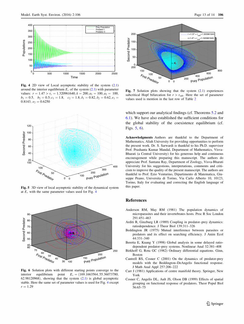
E� is stable for r[ rc ¼ 1:320961640 (cf. Figs. 4, 5 for local

stability and Fig. 6 for global stability). The system (2.1)

experiences a Hopf bifurcation when the parameter r crosses

the critical value rc from left to right, i.e., when r ¼ rc, all the

species coexist oscillating. Following the steps discussed in

Subsect. 6.1, we have found the value of P ¼1:042431405[ 0; which indicates that the obtained Hopf

bifurcation is a subcritical bifurcation (cf. Fig. 7).

It is observed that, if the interference coefficient b1

(interference effect on the first predator due to the pres-

ence of the second predator) increases it stabilizes the

system for b1 ¼ 0:7; while it is unstable at b1 ¼ 0:6:

When the parameter b1 exceeds its value 20, the first

predator population disappears from the system. Simi-

larly, the interference on the second predator due to the

presence of first predator, parameterized by b2 also plays

an important role to stabilize the system. If the interfer-

ence coefficient b2 increases it stabilizes the system for

b2 ¼ 0:6; while it is unstable at b2 ¼ 0:5: It also regulates

the existence of second predator in the system. As the

parameter b2 exceeds 20.9, the second predator population

gets extinguished.

Analogously, if the parameter d1; denoting the death rate

of the first predator increases then the size of the first

predator decreases as well as the second predator popula-

tion increases. If d1 decreases, the first predator population

increases and second predator population decreases. If the

death rate d1 is gradually increased to a certain level the

first predator population goes to extinction. A similar result

is observed for the case of the second predator’s death rate.

The above observations ensure that the model under con-

sideration is consistent with biological observations

(Figures are not reported here).

Concluding remarks

The problem described by the system (2.1) is well posed.

The x1; x2 and x3 axes are invariant under the flow of the

system. To our knowledge this is the first attempt to study

an ecological system with quasi-linear/bilinear growth of

the prey population. Generally, researchers only studied

biological model systems with logistic/linear growth of

prey population. One of the important results is that the

prey population becomes unbounded in absence of its

admissible predator in the long run. But in the presence of

predator the prey population can be bounded under


123

suitable combinations of system parameters. As a conse-

quence the total environmental population is bounded

above (cf. Subsect. 3.3). Therefore, any solution starting in

the interior of the first octant never leaves it. This

mathematical fact is consistent with the biological inter-

pretation of the system. Due to the inclusion of quasi-lin-

ear/bilinear growth of the prey population, the axial

equilibrium point is driven away by the system, a fact

Table 2 The set of system parameter (including the critical parameter rc) values and their corresponding Figures with description

No. Fixed parameters r Figures Description

1 r ¼ 1:37[ rc ¼ 1:320961640;

k ¼ 200; a1 ¼ 100; a2 ¼ 100;

b1 ¼ 0:5; b2 ¼ 0:5; c1 ¼ 1:8;

c2 ¼ 1:8; d1 ¼ 0:82; d2 ¼ 0:62;

e1 ¼ 0:8143; e2 ¼ 0:6250:

1.37 Fig. 1: (a)-(b) 2D view of Hopf

bifurcation

2 . . .. . .. . .. . .. . .. . .. . . 1.320961640 Fig. 2 Limit cycle

3 . . .. . .. . .. . .. . .. . .. . . r 2 ½0:8; 2:0 Fig. 3 Hopf bifurcation

(growth rate r vs.

population volumes)

4 . . .. . .. . .. . .. . .. . .. . . 1.4700000000 Fig. 4 2D view of local stability

5 . . .. . .. . .. . .. . .. . .. . . 1.4700000000 Fig. 5 3D view of local stability

6 . . .. . .. . .. . .. . .. . .. . . 1.4700000000 Fig. 6 Global stability

7

r ¼ 1:37; k ¼ 200;

a1 ¼ 100; a2 ¼ 100;

b1 ¼ 0:5; b2 ¼ 0:5;

c1 ¼ 1:8; c2 ¼ 1:8;

d1 ¼ 0:82; d2 ¼ 0:62;

e1 ¼ 0:8143; e2 ¼ 0:6250

rc ¼ 1:320961640;P ¼ 1:0424314050

Fig. 7 Subcritical Hopf bifurcation

Table 1 Schematic representation of our analytical findings

Equilibria Feasibility conditions/parametric restrictions Stability conditions/parametric restrictions Nature

E0 No conditions No conditions Unstable

E1 c1e1 [ d1, x11[ b1d1

c1e1�d1e1x11

þ x21[ kð1�b1e1Þ�a1

b1

LAS

E2 c2e2 [ d2, x12[ b2d2

c2e2�d2e2x12

þ x32[ kð1�b2e2Þ�a2

b2

LAS

E� x1� [ max a1d1

c1e1�d1; a2d2

c2e2�d2

n ok\min fa1 þ b1x2�; a2 þ b2x3�g LAS

E� .....................

ðiÞ r[ d1 þ d2; ðiiÞx11[

a2d2

c2e2 � d2

; ðiiiÞ x12[

a1d1

c1e1 � d1

Persistence

E� ..................... Stated in the Proposition 3.3 Boundedness

E� ..................... P[ 0 (cf. equation (6.15)) SHB

E� x1� [ max a1d1

c1e1�d1; a2d2

c2e2�d2

n oa1a2b1b2rk[ ðx1� þ kÞðwþ kÞ � ða1b1c2 þ a2b2c1Þ GAS

LAS locally asymptotically stable, GAS globally asymptotically stable, HB Hopf bifurcation, SHB subcritical Hopf bifurcation


123

which is rarely found in the modern research work on

mathematical biology. Thus, the prey population alone

cannot survive in stable condition without the predator

populations. Only the mutual interference between the

predators, which are parameterized by b1 and b2 can alone

stabilize the prey–predator interactions even when a quasi-

linear/bilinear intrinsic growth rate of prey population is

considered in the proposed mathematical model. These

parameters contribute in stabilizing prey–predator interac-

tions when only linear intrinsic growth rate is considered in

some mathematical models (cf. Dimitrov and Kojouharov

(2005)). There exist a balance between the predator’s need

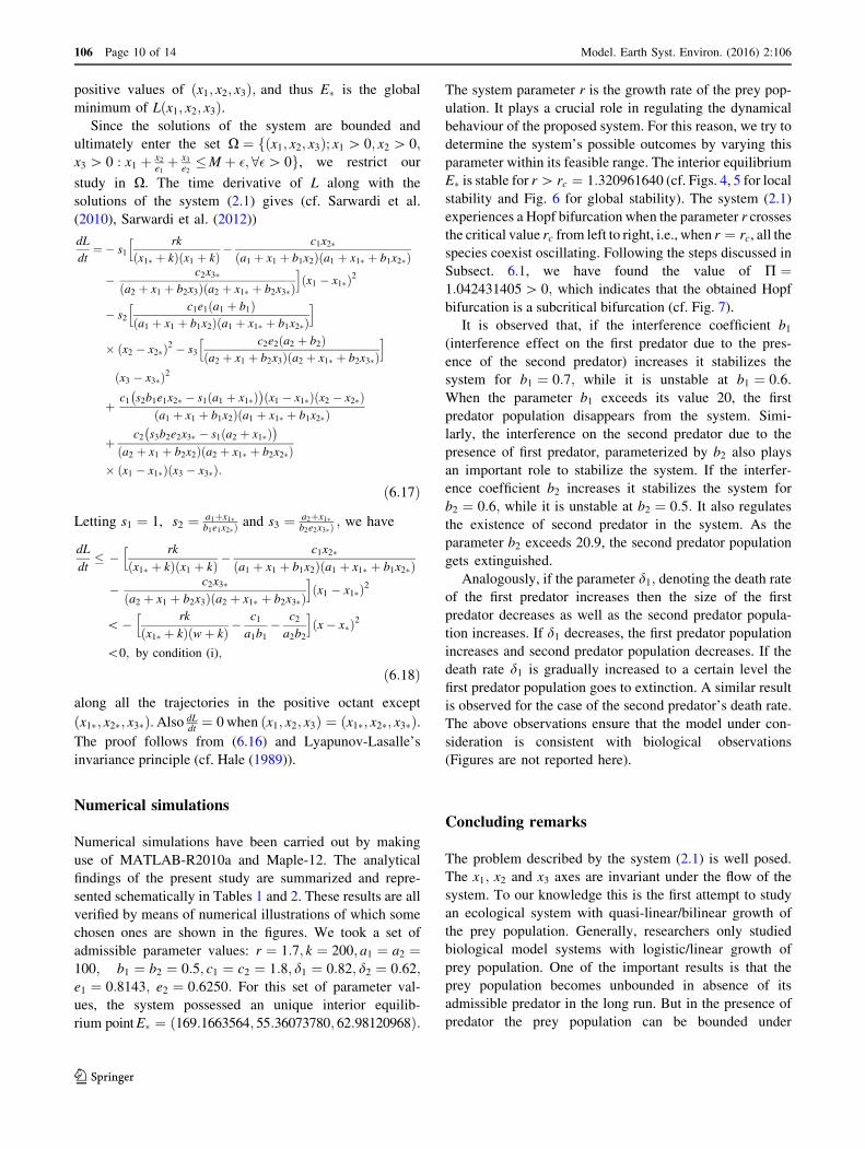
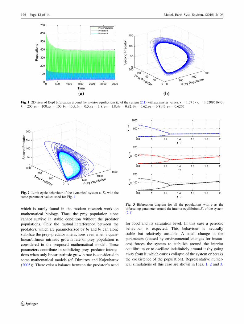
for food and its saturation level. In this case a periodic

behaviour is expected. This behaviour is neutrally

stable but relatively unstable. A small change in the

parameters (caused by environmental changes for instan-

ces) forces the system to stabilize around the interior

equilibrium or to oscillate indefinitely around it (by going

away from it, which causes collapse of the system or breaks

the coexistence of the population). Representative numer-

ical simulations of this case are shown in Figs. 1, 2 and 3,

(a)

0 500 1000 1500 2000 2500 30000

100

200

300

400

500

600

700

Time

Pop

ulat

ions

Prey PopulationPredator IPredator II

(b)

0200

400600

050

100150

2000

50

100

150

Prey PopulationFirst Predator

Sec

ond

Pre

dato

r

Fig. 1 2D view of Hopf bifurcation around the interior equilibrium E� of the system (2.1) with parameter values: r ¼ 1:37[ rc ¼ 1:320961640;k ¼ 200; a1 ¼ 100; a2 ¼ 100; b1 ¼ 0:5; b2 ¼ 0:5; c1 ¼ 1:8; c2 ¼ 1:8; d1 ¼ 0:82; d2 ¼ 0:62; e1 ¼ 0:8143; e2 ¼ 0:6250

0

500

1000

1500

0

100

200

3000

50

100

150

200


Sec

ond

Pre

dato

r

Fig. 2 Limit cycle behaviour of the dynamical system at E� with the

same parameter values used for Fig. 1

0.8 1 1.2 1.4 1.6 1.8 20

500

1000

r →

x1

→

0.8 1 1.2 1.4 1.6 1.8 20

100

200

r→

x2

→

0.8 1 1.2 1.4 1.6 1.8 20

100

200

r →

x3

→

Fig. 3 Bifurcation diagram for all the populations with r as the

bifurcating parameter around the interior equilibrium E� of the system

(2.1)


123

which support our analytical findings (cf. Theorems 5.2 and

6.1). We have also established the sufficient conditions for

the global stability of the coexistence equilibrium (cf.

Figs. 5, 6).

Acknowledgments Authors are thankful to the Department of

Mathematics, Aliah University for providing opportunities to perform

the present work. Dr. S. Sarwardi is thankful to his Ph.D. supervisor

Prof. Prashanta Kumar Mandal, Department of Mathematics, Visva-

Bharati (a Central University) for his generous help and continuous

encouragement while preparing this manuscript. The authors do

appreciate Prof. Santanu Ray, Department of Zoology, Visva-Bharati

University for his suggestions, interpretations, comments and criti-

cism to improve the quality of the present manuscript. The authors are

thankful to Prof. Ezio Venturino, Dipartimento di Matematica, Giu-

seppe Peano, Universita di Torino, Via Carlo Alberto 10, 10123,

Torino, Italy for evaluating and correcting the English language of

this paper.

References

Anderson RM, May RM (1981) The population dynamics of

microparasites and their invertebrates hosts. Proc R Soc London

291:451–463

Arditi R, Ginzburg LR (1989) Coupling in predator–prey dynamics:

ratiodependence. J Theor Biol 139:311–326

Beddington JR (1975) Mutual interference between parasites or

predators and its effect on searching efficiency. J Anim Ecol

44:331–340

Beretta E, Kuang Y (1998) Global analysis in some delayed ratio-

dependent predator–prey systems. Nonlinear Anal 32:381–408

Birkhoff G, Rota GC (1982) Ordinary differential equations. Ginn,

Boston

Cantrell RS, Cosner C (2001) On the dynamics of predator-prey

models with the Beddington–DeAngelis functional response.

J Math Anal Appl 257:206–222

Carr J (1981) Applications of centre manifold theory. Springer, New

York

Cosner C, Angelis DL, Ault JS, Olson DB (1999) Effects of spatial

grouping on functional response of predators. Theor Popul Biol

56:65–75

0 500 1000 1500 2000 25000

50

100

150

200

250

300

350

400

Time

Pop

ulat

ions

Prey PopulationPredator IPredator II

Fig. 4 2D view of Local asymptotic stability of the system (2.1)

around the interior equilibrium E� of the system (2.1) with parameter

values: r ¼ 1:47[ rc ¼ 1:320961640; k ¼ 200; a1 ¼ 100; a2 ¼ 100;b1 ¼ 0:5; b2 ¼ 0:5; c1 ¼ 1:8; c2 ¼ 1:8; d1 ¼ 0:82; d2 ¼ 0:62; e1 ¼0:8143; e2 ¼ 0:6250

0100

200300

400

0

50

100

15020

40

60

80

100

120


Sec

ond

Pre

dato

r

Fig. 5 3D view of local asymptotic stability of the dynamical system

at E� with the same parameter values used for Fig. 4

100150

200250

3040

5060

708040

50

60

70

80

90

Prey Population

← E*

← E*

← E*

← E*

← E*

← E*

← E*

← E*

First Predator

Sec

ond

Pre

dato

r

Fig. 6 Solution plots with different starting points converge to the

interior equilibrium point E� ¼ ð169:1663564; 55:36073780;62:98120968Þ; showing that the system (2.1) is global asymptotic

stable. Here the same set of parameter values is used for Fig. 4 except

r ¼ 1:29

0200

400600

800

050

100150

2000

50

100

150

200

Prey Population

← E*

← E*

First Predator

Sec

ond

Pre

dato

r

r =1.37 > rsub

=1.320961640

r=1.47 > rsub

=1.320961640

Fig. 7 Solution plots showing that the system (2.1) experiences

subcritical Hopf bifurcation for r[ rsub: Here the set of parameter

values used is mention in the last row of Table 2


123

Cui J, Takeuchi Y (2006) Permanence, extinction and periodic

solution of predator–prey system with Beddington–DeAngelis

functional response. J Math Anal Appl 317:464–474

Curds CR, Cockburn A (1968) Studies on the growth and feeding of

Tetrahymena pyriformis in axenic and monoxenic culture. J Gen

Microbiol 54:343–358

DeAngelis RA, Goldstein RA, Neill R (1975) Ecology 56:881–892

Dimitrov DT, Kojouharov HV (2005) Complete mathematical

analysis of predator–prey models with linear prey growth and

Beddington–DeAngelis functional response. Appl Math Comp

162:523–538

Freedman HI (1990) A model of predator–prey dynamics modified by

the action of parasite. Math Biosci 99:143–155

Gard TC, Hallam TG (1979) Persistence in Food web-1, Lotka-

Volterra food chains. Bull Math Biol 41:877–891

Hadeler KP, Freedman HI (1989) Predator–prey populations with

parasitic infection. J Math Biol 27:609–631

Hale JK (1989) Ordinary differential equations. Krieger Publisher

Company, Malabar

Haque M, Venturino E (2006) Increase of the prey may decrease the

healthy predator population in presence of a disease in the

predator. Hermis 7:39–60

Haque M, Venturino E (2006) The role of transmissible diseases in

the Holling–Tanner predator–prey model. Theor Popul Biol

70:273–288

Hassell MP, Varley GC (1969) New inductive population model for

insect parasites and its bearing on biological control. Nature

223:1133–1137

Hethcote HW, Wang W, Ma Z (2004) A predator–prey model with

infected prey. Theor Popul Biol 66:259–268

Huo HF, Li WT, Nieto JJ (2007) Periodic solutions of delayed

predator–prey model with the Beddington–DeAngelis functional

response. Chaos Solitons Fractals 33:505–512

Hwang TW (2003) Global analysis of the predator–prey system with

Beddington–DeAngelis functional response. J Math Anal Appl

281:395–401

Kar TK, Gorai A, Jana S (2012) Dynamics of pest and its predator

model with disease in the pest and optimal use of pesticide.

J Theor Biol 310:187–198

Ma WB, Takeuchi Y (1998) Stability analysis on predator–prey

system with distributed delays. J Comput Appl Math 88:79–94

Salt GW (1974) Predator and prey densities as controls of the rate of

capture by the predator Didinium nasutum. Ecology 55:434–439

Sarwardi S, Haque M, Venturino E (2010) Global stability and

persistence in LG-Holling type-II diseased predators ecosystems.

J Biol Phys 37:91–106

Sarwardi S, Mandal PK, Ray S (2012) Analysis of a competitive

prey–predator system with a prey refuge. Biosystems

110:133–148

Sarwardi S, Mandal PK, Ray S (2013) Dynamical behaviour of a two-

predator model with prey refuge. J Biol Phys 39:701–722

Venturino E (1995) Epidemics in predator–prey models: disease in

prey, in mathematical population dynamics. Analysis of hetero-

geneity 1. In: Arino O, Axelrod D, Kimmel M, Langlais M (eds),

pp 381–393

Wiggins S (2003) Introduction to applied nonlinear dynamical

systems and Chaos, 2nd edn. Springer, New York

Xiao Y, Chen L (2001) Modeling and analysis of a predator–prey

model with disease in prey. Math Biosci 171:59–82


123

dynamical behaviour of an ecological system with

Documents