dynamic wacc: re-enrichment of discounted cash flow

DYNAMIC WACC: RE-ENRICHMENT OF

DISCOUNTED CASH FLOW VALUATION TECHNIQUE

SKRIPSI

Presented in partial fulfillment of the requirements for

The Bachelor’s Degree in Accounting

By:

Nico

008201500065

FACULTY OF BUSINESS

ACCOUNTING STUDY PROGRAM

PRESIDENT UNIVERSITY

CIKARANG, BEKASI

2019

i

PLAGIARISM CHECK RESULT

DYNAMIC WACC: RE-ENRICHMENT OF DISCOUNTED CASH FLOW VALUATION TECHNIQUE

x

ACKNOWLEDGEMENT

With blessing of God, the researcher has finally finished the skripsi entitled Dynamic

WACC: Re-enrichment of Discounted Cash Flow Valuation Technique. This page

thus is entitled to all of the people, friend, and colleagues who have been supporting

the researcher in finishing the skripsi. Without their supports, it is impossible for the

researcher to get to this point.

The researcher would like to show high appreciation and gratitude to all of the

individuals who are involved in the process of this skripsi writing, those individuals

are:

1. Dr. Josep Ginting, CFA as the skripsi advisor who has been guiding the

researcher to explore further about the art of researching and logical thinking

in research process,

2. The researcher’s beloved family member who have been encouraging the

researcher to do better every time the burnout comes during the skripsi writing

process,

3. Friends and colleagues from President University who have become the

source of motivation for the researcher. The researcher will never forget the

time when we motivate each other to achieve the goal together,

4. All of the examiners, lecturers, and staffs whom the researcher cannot

mention one by one, without your support, it is impossible for the researcher

to finally achieve this point.

May all of us live a happy life and achieve the goals that we have set. The researcher

will not forget the merits and contribution that you have done to the researcher.

Cikarang, 1st February 2019

Nico

xi

TABLE OF CONTENTS

PLAGIARISM CHECK RESULT ............................................................................. i

DECLARATION OF ORIGINALITY .................................................................. viii

PANEL OF EXAMINERS APPROVAL ................................................................. ix

ACKNOWLEDGEMENT .......................................................................................... x

TABLE OF CONTENTS ........................................................................................... xi

LIST OF TABLES AND FIGURES ....................................................................... xiii

ABSTRACT .............................................................................................................. xiv

INTISARI ................................................................................................................... xv

CHAPTER I: INTRODUCTION .............................................................................. 1 1.1. Background of the Study .................................................................................... 1

1.2. Problem Statement .............................................................................................. 5

1.3. Study Objectives ................................................................................................. 7

1.4. Significant of the Study ...................................................................................... 8

1.5. Organization of Writing ..................................................................................... 9

CHAPTER II: LITERATURE REVIEW ............................................................... 11 2.1. Definition of Value and Valuation ................................................................... 11

2.2. Variety of Techniques in Valuation ................................................................. 14

2.3. Valuation Using Discounted Cash Flow Technique ........................................ 18

2.4. Forecasting Cash Flows .................................................................................... 23

2.5. Capital Structure and Cost of Capital ............................................................... 26

2.6. Cost of Capital, Pecking Order Theory, and DCF Problems ........................... 30

2.7. Proposed Valuation Technique ......................................................................... 32

CHAPTER III: METHODOLOGY ........................................................................ 36

3.1. Research Design ............................................................................................... 36

3.2. Sampling Design .............................................................................................. 40

3.3. Data Collection and Data Processing ............................................................... 44

3.3.1. Conducting Preliminary Filtering and Testing .......................................... 45

xii

3.3.2. Classifying Financial Informations into Forecasting Format .................... 46

3.3.3. Forecasting the Explicit and Post-Horizon FCF ........................................ 47

3.3.4. Determining the WACC of Each Model ................................................... 49

3.3.5. Discounting FCF to NPV for Each Model ................................................ 50

3.3.6. Comparing Fair Value per Stock for Each Model with Market ................ 51

3.4. Statistical Analysis ........................................................................................... 52

CHAPTER IV: DATA ANALYSIS AND INTERPRETATION OF RESULTS 55

4.1. Data Description ............................................................................................... 55

4.2. Results and Discussion ..................................................................................... 59

4.2.1. Data Interpretation and Theoretical Integration ........................................ 59

4.2.2. Data Validation Result through Quantitative Approach ............................ 65

CHAPTER V: CONCLUSION AND RECOMMENDATION ............................ 69

5.1. Conclusion ........................................................................................................ 69

5.2. Limitations and Recommendations .................................................................. 70

5.2.1. Limitations of Dynamic WACC Model .................................................... 70

5.2.2. Recommendations for Future Research ..................................................... 71

5.3. Implications ...................................................................................................... 72

REFERENCES .......................................................................................................... 74

APPENDIX ................................................................................................................ 97

xiii

LIST OF TABLES AND FIGURES

Table 1 – Representative Samples Chosen ............................................................. 55

Table 2 – Descriptive Statistics of Actual Market Price ........................................ 55

Table 3a – Traditional WACC DCF Valuation Model .......................................... 57

Table 3b – Dynamic WACC DCF Valuation Model .............................................. 57

Table 4a – Traditional WACC Model and Market Price Comparison ............... 58

Table 4b – Dynamic WACC Model and Market Price Comparison.................... 58

Table 5a – Error in Traditional WACC Model ..................................................... 59

Table 5b – Error in Dynamic WACC Model ........................................................ 59

Figure 1 – Box Plot of Actual Market Price .......................................................... 56

xiv


ABSTRACT

The current and widely used traditional Discounted Cash Flows (“DCF”) valuation

technique implements constant Weighted Average Cost of Capital (“WACC”) as

discount factor in estimating the company’s value. However, previous studies in

firms’ financing behavior have shown that the implementation of constant WACC is

not applicable to real finance practice. Moreover, the recent studies in finance have

highlighted the importance of internal financing towards the financing behavior and

WACC of the company. In this study, the researcher would like to introduce new

DCF valuation technique which implements the dynamic WACC rather than the

constant one by emphasizing on the impact of a firm’s internal financing capability in

accordance to Pecking Order Theory. Based on the Root Mean Square Error

(“RMSE”) and Standard Error (“SE”) indicated by the statistical analysis from eight

public-listed non-financing companies from various industry sectors in Indonesia

Stock Exchange, the implementation of the dynamic WACC has better accuracy in

estimating the company’s value as indicated by the share price, aligned with the

Pecking Order Theory. Future research should develop and enrich the currently

implemented traditional DCF valuation technique from other dimensions, such as the

Free Cash Flows and the Terminal Value.

Keywords: DCF, WACC, Pecking Order Theory, Internal Financing

xv


INTISARI

Teknik penilaian tradisional Discounted Cash Flows (“DCF”) yang saat ini

digunakan dengan luas mengimplementasikan Weighted Average Cost of Capital

(“WACC”) yang konstan sebagai faktor diskonto dalam mengestimasikan nilai

perusahaan. Namun, penelitian-penelitian sebelumnya telah menunjukan bahwa

implementasi WACC yang konstan tidak berlaku untuk praktek keuangan yang nyata

di lapangan. Selain itu, penelitian terkini di bidang keuangan telah menekankan

pentingnya pendanaan internal terhadap perilaku pendanaan dan WACC perusahaan.

Dalam penelitian ini, peneliti ingin memperkenalkan teknik penilaian DCF baru yang

mengimplementasikan WACC yang dinamis daripada konstan dengan menekankan

pada pengaruh kemampuan pendanaan internal perusahaan berdasarkan Pecking

Order Theory. Berdasarkan analisa statistik Root Mean Square Error (“RMSE”) dan

Standard Error (“SE”) yang dilakukan terhadap delapan perusahaan publik non-

keuangan di Bursa Efek Indonesia yang berasal dari beragam sektor industri,

implementasi WACC yang dinamis memiliki akurasi yang lebih baik dalam

mengestimasikan nilai perusahaan sebagaimana diindikasikan dengan harga saham,

sejalan dengan Pecking Order Theory. Penelitian selanjutnya seharusnya dapat

mengembangkan dan memperkaya teknik penilaian DCF tradisional dari dimensi-

dimensi lain, seperti Free Cash Flow dan Terminal Value.

Keywords: DCF, WACC, Pecking Order Theory, Internal Financing

1

CHAPTER I:

INTRODUCTION

1.1. Background of the Study

Valuation is one of the most commonly discussed subject in finance study and

it plays vital roles in the practices of finance fields. Damodaran (2012) stated

that valuation is commonly used in portfolio management, acquisition

analysis and corporate finance. In regards with its practice in finance field, the

studies on valuation have been also developed rapidly. Therefore, it is not

surprising that there exists various valuation techniques in finance practice. In

his paper, Fernández (2007) classified the currently implemented valuation

techniques into six which are the Balance Sheet technique, Income Statement

technique, Mixed technique, Discounted Cash Flows (“DCF”) technique,

Value Creation technique, and Options technique. Each of the valuation

technique implements different assumptions and framework in estimating the

value of an asset.

Among all of the valuation techniques mentioned above, one of the most

commonly accepted valuation technique is the DCF technique (Fernández,

2007). While Balance Sheet and Income Statement techniques focus on the

accounting earnings reported in the financial statements, DCF technique is

2

more focused in measuring the economic profit generated by the company.

Miller and Modigliani (1958) explained that the earnings generated from an

asset must be compared with the costs to obtain the respective earnings since

that will determine the “true worth” of the earnings. This concept was then

implemented in the widely used DCF valuation technique in current days.

In the DCF technique, the firm’s value is equivalent to the present value of its

expected free cash flows. This approach requires free cash flows forecasts

which are the proxies of the firm’s operation in future. After the free cash

flows have been estimated, the free cash flows will be discounted to Present

Value by using the Weighted Average Cost of Capital (“WACC”) to arrive at

the firm’s value. According to Fernández (2007), adjusting the forecasted free

cash flows with WACC to derive firm’s value reflects the “true” return for the

firm’s by utilizing the combination of debt and equity as capital. Based on the

aforementioned explanation, the implementation of DCF technique requires

quantitative process in determining the firm’s value.

Though the DCF technique involves quantitative process in determining the

firm’s value, it should be noted that the DCF method has limitation due to its

implied assumptions. One of the limitations implemented in the DCF

valuation technique is the application of WACC which then will be used as

the discount factor in the valuation technique. Since the current DCF model

3

adopts the Miller and Modigliani (1958) framework, current DCF model also

assumes that the WACC used will be constant throughout the firms’ life

cycle. This was aligned with the capital structure theory proposed by Miller

and Modigliani (1958) which stated that under perfect market condition the

changes in financing mix will not affect the WACC. The capital structure

theory proposed by Miller and Modigliani (1958) thus referred as the

“Irrelevancy Theory”.

The implementation of this constant WACC in DCF valuation technique thus

raises questions regarding the applicability of DCF model in the current

market. Myers (2001) argued that should a firm’s WACC remain constant in

spite of its financing mix, a firm will not generate any innovation in financing

instruments and there will be no development in financing strategies.

However, the proof of existing major development in the financing innovation

has become the evidence that firms consider the financing mix in order to

maximize its performance and therefore, it shows that there is a limitation in

the concept of Miller and Modigliani (1958). In addition to that, Vélez-Pareja,

Ibragimov, and Tham (2008) found out that the constant WACC does not hold

true since the WACC also depends on the discount rate of the tax shield.

While the DCF technique focuses on the firms’ financing mix which is

constituted by the composition of external financing instruments, such as debt

4

and equity instruments, there exists increasing attention in the internal

financing of the company as well. This can be seen from the research

conducted by Vogt (1994) which proved that the internal financing

capabilities could affect the investment and financing decisions of the firms.

Ross, Westerfield, Jaffe, Lim, and Tan (2015) also pointed out about the Cost

of Retained Earnings (“Kr”) which is resulted from the internal financing

capability as the component which constitutes the WACC. These literatures

imply that there should be a consideration of internal financing component in

calculating the WACC in the DCF valuation technique.

.

The current studies in valuation field are dominated with the comparative

researches which focus on proving the superiority of one valuation technique

over the others, such as the studies conducted by Sayed (2017), Courteau,

Kao, and Richardon (2000), Francis, Olson, and Oswald (2000), and Penman

and Sougiannis (1998). According to Lundholm (2001), the future research in

the valuation field must not focus on comparing the valuation techniques but

concern more on the methods to increase the accuracy of valuation technique.

The researcher believes that each of the existing valuation technique provides

estimated firm’s value based on its implied assumptions. However, the issue

with the valuation study field is to analyze whether the assumptions implied

by each valuation technique are still applicable in the practical world and

5

whether there should be any re-enrichment that can be done to increase the

accuracy of the traditional model. The study conducted by Vélez-Pareja et al

(2008) integrated the Tradeoff Theory into the traditional DCF model and

concluded that the WACC shall follow the principle of tax shield benefits. It

is interesting for the researcher to analyze the WACC assumptions from the

perspective of other capital structure theory, especially by integrating the

internal financing components into the DCF valuation model. This could

provide new framework in valuing the firms and develop the traditional DCF

model.

1.2. Problem Statement

Myers (2001) pointed out that the implementation of constant WACC in DCF

valuation technique may not be congruent with the real economic

environments that the market faces. This statement then is strengthened by the

inquiry of Vélez-Pareja et al (2008) which stated that WACC cannot be

constant due to the tax shield considerations.

The issue to be highlighted in this study would be the incorrect application of

WACC in DCF valuation. By using the constant discount rate for discounting

the expected free cash flows, it implies that the company will use the same

capital structure throughout the firm’s life. However, it should be noted that

6

the net income generated in the current year will increase the portion of equity

(internal financing capability), changing the capital structure and therefore

changing the cost of capital (WACC) to be then used as the discount factor in

discounting the free cash flows to the firm’s value. While the portion of equity

increase, under the constant cost of capital assumption, the company will be

assumed to issue more debt with the same cost of debt to maintain the current

cost of capital. However, it should be noted that issuance of debt would

depend on the company’s action and would be a matter of bias in the cash

flows forecast of the firm.

There raises questions regarding the capability for the debt holders to obtain

the exact same cost of debt in the future and the allocation of the debt

financing resources to the company’s investment. In accordance with the

Pecking Order Theory introduced by Myers (1984), for companies that have

better internal financing capability, the issuance of new debt will not be seen

as rational since the management of the firms could employ the internal

financing resources for the investment projects and therefore could conduct an

investment with lower-risk.

To sum it all, this study would like to highlight the problem of incorrect

discount factor errors due to the constant WACC implementation in DCF

valuation technique and offers new valuation model which covers the

7

weakness of the traditional DCF model. Since internal financing capability is

also one of the drivers which affect WACC, the researcher would like to

develop new constructed valuation model which focuses on the influence of

internal financing capability towards the WACC.

1.3. Study Objectives

Based on the research problems mentioned in the previous section, the

objective of this research is to develop the concept of DCF practice and

implementation which adopts the capital structure theory of Miller and

Modigliani (1958) by addressing the constant WACC problem so that the

current valuation model would be more comprehensive and accurate.

As for the constant WACC as discount factor problem, the researcher would

like to develop a model in which the WACC as discount factor will be

assumed to be changed over the forecast period by referring the equity capital

component as the function of previous equity. WACC is constructed through

the elements of capital structure and in this study, the researcher will focus on

the influence of changes in internal financing capability as the variable which

will affect the WACC.

8

This study aims to provide the readers about the logical framework behind the

traditional DCF valuation technique and the implied capital structure theory

and provide sufficient evidence regarding the better applicability of the

dynamic WACC model in terms of accuracy.

1.4. Significance of the Study

Recalling that the valuation process is one of the core subjects in the finance

study, the result of this research would be beneficial for both academicians

and practitioners in finance fields.

The result of this research would provide more insights for the academicians

regarding the exploration of alternative element in the DCF analysis approach

in the business valuation and therefore would enrich the finance literatures,

especially in terms of DCF valuation approach.

In addition to that, by emphasizing on the development of dynamic WACC,

the managements of companies will be able to utilize more comprehensive

version of DCF technique, resulting in better decision making in the business

management process.

9

The development of DCF technique offered in this research will also be

beneficial for the shareholders who provide capital to the business or

companies. The shareholders will be able to have a more accurate target value

so that they could maximize their potential return and avoid the unfavorable

investments.

Since the valuation process is also one of the core parts in the merger and

acquisition, the development of DCF approach which is widely used in the

merger and acquisition (“MnA”) deals will provide better insights for the

public accountants regarding the assessment of the fairness in the merger and

acquisition deal which then would affect the goodwill account as reported in

the Statement of Financial Position of respective company.

1.5. Organization of Writing

This research paper is organized into five chapters from Chapter I until

Chapter V. Chapter I provides the introduction about the research problems

and the background which motivates the author to write this research paper.

Chapter II provides the literature reviews which emphasize the development

of prior theories regarding the concept of valuation and DCF approach and

supporting theories in the new valuation model proposed in this study. The

proposed model will be explained after the literature reviews in “Proposed

10

Method” section. Chapter III provides the methodology including the

sampling and data processing methods in testing the validity and accuracy of

proposed method mentioned in prior section. Chapter IV provides the result of

the data processing as mentioned in prior chapter and interprets the

quantitative result of data processing. Chapter V provides the conclusion

regarding the research, limitations of the research, and the direction for the

future research.

11

CHAPTER II:

LITERATURE REVIEW

2.1. Definition of Value and Valuation

Valuation is not a new topic in the accounting and finance field of studies. It is

widely used for the purpose of measuring and understanding the value of an

asset, investment, or even a company. According to Koller, Goedhart, and

Wessels (2010), value is interpreted as the defining measurement dimension in

the market’s economy. It integrates the long-term perspective and expectations

of the market towards an asset. The term “value” can be interpreted simply as

the “true worth” of an asset. Damodaran (2012) argued that understanding the

true value of an asset is crucial since an investor shall not purchase an asset at

the price beyond its expected value.

In determining the true worth of an asset, there will be a quantitative process to

be utilized in order to estimate the value of respective asset which is referred as

“valuation”. Damodaran (2012) stated that different assets require different

information inputs and valuation techniques in order to derive the estimated

value. For example, valuing real estate property will require different details of

12

information inputs and different valuation formats from the process of valuing

publicly traded stocks.

As what has been mentioned on the first paragraph, understanding the value of

an asset would be critical since it would provide insights for investors regarding

the “ceiling” or limit that investor should pay in order to acquire those assets.

According to Damodaran (2012) and Koller, et.al (2010), there are some

practical roles of valuation in the business fields, which are:

a. In the portfolio management, understanding the value of an asset would

be useful for the long-term investors who are more focused on the firm-

specific valuation rather than the market valuation. It plays central role

for the fundamental analyst and provides peripheral role for the technical

analyst.

b. In the merger and acquisition analysis, valuation will provide the

bidding firm the fair value of the target firm before making the bid to

acquire the target firm, while for the target firm itself, the valuation will

provide them insights regarding minimum price before accepting the

deal offered by the bidding firm based on the fair value of the firm.

c. In corporate finance, understanding the value of the managed firm is

crucial since the main objective of the corporate finance is to maximize

the value of the firm. By utilizing the valuation, the managers could

13

assess the impact of their financial policies, operational policies, and

corporate strategies towards the firm’s value.

The roles of valuation are crucial not only for the practice in finance field but

also for the practice in accounting field. Since the valuation affects the financial

substance of transactions, it will directly affects the way of those transactions to

be reported which would be the main concern of accounting field.

In accordance with the Conceptual Framework of Financial Reporting, one of

the crucial issue in the accounting field is the measurement or valuation of

accounting items so that all of the economic transactions can be presented in

financial statements at the fair value. After the adoption of International

Financial Reporting Standards (IFRS) in accounting practice, the fair value

concept which is explained in the International Accounting Standard (IAS) 39 is

heavily implemented in the financial reporting since it would increase the value

relevance of the informations provided in the financial reports for the decision

making process done by the users. In Indonesia which adopts the IFRS, the

importance of valuation is also recognized through the Pernyataan Standar

Akuntansi Keuangan (PSAK) 68 regarding the Fair Value Measurement.

It should be noted that even though valuation involves complex and analytical

process in order to derive the expected value of an asset, there are some pitfalls

that must be taken into the considerations according to Damodaran (2012):

14

a. Valuation is not a pure science in which its proponents make it out to be

or will result in a pure objective true value. Even though the valuation

process involves quantitative model, however, the information inputs

might be colored with highly subjective bias. Therefore, it is important

to reduce the bias in the process of valuing an asset,

b. Valuation process is not timeless which means the derived value from

previous valuation may be changed due to the new information reveal in

the market which then will affect the perspective of an asset’s value,

c. Valuation doesn’t provide precise value since all of the inputs are in

form of estimation as well,

d. Good valuation doesn’t require complex quantitative model. Providing

too much financial details may result in the bias of input errors as well.

For the simplicity purposes, Koller, et al (2010) pointed out that the key

drivers of value creation are the growth and return on invested capital,

e. Good valuation shall not ignore the perspectives of other investors in the

current market and,

f. The most important thing about valuation is the process rather than the

outputs.

2.2. Variety of Techniques in Valuation

15

Recalling that different assets require different information inputs and formats,

the valuation process can be classified into various techniques. Every valuation

techniques implies different concepts and approaches in order to estimate the

value of an asset, investment, or company. Based on the valuation objects and

techniques, Fernández (2007) classified the valuation techniques as follow:

a. Balance Sheet Technique

This technique implies that the value of a company would be equivalent

to the amount that is reflected in the company’s balance sheet without

considering the market’s condition, human resources, or other

organizational issues in the future which are not depicted in the

company’s balance sheet. There are so many indicators that can be used

for this balance sheet technique and one of the most common indicator

would be the book value of the company which is defined as the

difference between the total assets and liabilities.

b. Income Statement Technique

This techniques implies that the value of the company would be shown

by the income indicators such as earnings, sales, or other indicators.

Unlike balance sheet technique which is derived from pure accounting

value, the income statements techniques emphasized on the comparison

16

of multiples by comparing the accounting income indicators with the

other relevant market indicator, commonly market price to derive a ratio.

It implies that the value of a company would be at the multiples of its

income indicators.

Until now, this technique is still used for providing quick valuation

insights regarding a company due to its simplicity in process. One of the

most commonly used multiple in finance practice would be the Price-

Earning Ratio (PER) in which the share value of a company would be the

multiples of its earnings.

c. Mixed (Goodwill) Valuation Technique

Since balance sheet method don’t provide insights regarding the impact

of non-accounting items towards the value of the company, the mixed

valuation method is formulated. This techniques implies that the value of

a company is equivalent to the sum of its accounting net assets value and

its goodwill. The “classic” goodwill valuation is expressed in form of the

equation below:

𝑽 = 𝐀 + (𝒏 × 𝑩) or 𝑽 = 𝐀 + (𝒛 × 𝑭)

Where A= net assets value, n=coefficient (1.5-3), B= net income,

z= percentage of sales, F= sales turnover.

17

The first formula is commonly used for manufacturing companies while

the second formula is commonly used for retail companies. This

techniques implies that the goodwill of a company is derived from a

multiples of an economic indicator and will be added to the substantial

net asset value.

d. Discounted Cash Flows Technique

This technique seeks to determine company’s value by forecasting the

expected cash flows in the future and then discount them to the present

value by using certain discount factor which reflects the risk.

Up to now, this method is the most commonly used in the fundamental

analysis due to its rational concept and its generality to be used in valuing

not only equity instruments or companies but also most of the financial

instruments including debt instruments.

The discounted cash flow valuation formula is depicted as follow:

𝑉 =𝐶𝐹1

(1 + 𝑘)1 +𝐶𝐹2

(1 + 𝑘)2 +𝐶𝐹3

(1 + 𝑘)3 + ⋯+𝐶𝐹𝑛 + 𝐶𝑅𝑛(1 + 𝑘)𝑛

Where V= value of the company, CF= expected cash flows in the future,

k= discount factor, n= forecast period, and CR= terminal cash flow.

e. Value Creation Technique

This technique implies that the value of a company could be assessed

from the excess of returns it generated from the capital employed in its

18

operation. One of the most common indicators to be used in this

technique is the Economic Value Added (EVA) indicator. According to

Chen and Dodd (1997), the formula of EVA is depicted as follow:

𝐸𝑉𝐴 = (𝑅𝑜𝐼𝐶 − 𝐶𝑜𝐶) × 𝐶

Where EVA= Economic Value Added, RoIC= return on invested capital,

CoC= Cost of Capital, C= total capital employed

This EVA valuation though cannot be used as the proxy in the market

price like Discounted Cash Flow Technique. It only provides a sole

amount which then can be used to determine the performance of the

company.

f. Black-Scholes-Merton Technique

This technique is only applicable to the option instrument in which the

option price will be affected by the underlying instruments and therefore

requires considerations regarding the changes in the underlying option

instruments. After the establishment of Black-Scholes model in the

option pricing in 1973, Merton (1976) provided additional insights

regarding the option pricing for discontinuous stock price return and

creating Black-Scholes-Merton model. The formula is depicted as below:

𝐹(𝑆, 𝜏) = �𝑃𝑛(𝜏)𝜀𝑛{𝑊(𝑉𝑛, 𝜏;𝐸,𝜎2, 𝑟)}∞

𝑛=0

19

2.3. Valuation Using Discounted Cash Flow Technique

As mentioned in the previous section, Discounted Cash Flow (DCF) technique

implies that the value of a company is derived by discounting the expected cash

flows in the future by using certain discount factor which reflects the risk. The

formula of DCF technique is depicted as follow:

𝑉 =𝐶𝐹1

(1 + 𝑘)1 +𝐶𝐹2

(1 + 𝑘)2 +𝐶𝐹3

(1 + 𝑘)3 + ⋯+𝐶𝐹𝑛 + 𝐶𝑅𝑛

(1 + 𝑘)𝑛

Where V= value of the company, CF= expected cash flows in the future,

k= discount factor, n= forecast period, CR= terminal cash flow.

The core concept of DCF is aligned with the economic theory introduced by

Miller and Modigliani (1958) which stated that the value of an asset should be

perceived from economic perspective rather than solely accounting perspective

by taking into the account the risk factor.

Based on the formula depicted above, the value derived from the DCF valuation

technique is influenced by several factors which are:

a. Forecasted Cash Flow, this variable is the expected cash flows in the

future which act as numerators in the DCF formula. To be specific,

the forecasted cash flows discussed in DCF formula are the Free Cash

Flows which are derived from the reconciliation of some accounting

items. In the implementation of cash flows forecast, the free cash

20

flows would be forecasted for several period which is referred by

Jennergren (2008) as the explicit period while the rest of free cash

flows will be presented in terms of lump sum which reflects the post-

horizon period of free cash flows. Depending on the type of DCF

valuation implemented, the reconciliation process to arrive at the free

cash flows amount will be different.

b. Discount Factor, this variable reflects the risk in respect to the

forecasted free cash flows. By implementing the discount factor as

the denominator, the expected free cash flows in the future will be

brought back to its present value which represents the value of the

future free cash flows as in the present. Depending on the type of

DCF valuation implemented, the determination of the discount factor

will be different as well.

c. Period, this variable shows the so-called “explicit” cash flow period

in which the free cash flows are predicted explicitly by using given

assumptions. The remaining of the forecasted free cash flows will be

presented in lump sum with the basis of the latest forecasted free cash

flows in the explicit period. The lump-sum amount which represents

the rest of the forecasted cash flows is referred by Jennergren (2008)

as the post-horizon forecasted cash flows period.

21

According to Damodaran (2012), the Discounted Cash Flows valuation

technique may also be classified into two techniques in accordance with the

purpose of the valuation, they are Free Cash Flows to Equity (FCFE) technique

and Free Cash Flows to Firm (FCFF) technique. Both of those DCF techniques

provides different approach in deriving the value of a company, however,

theoretically speaking, the value derived from both approach shall be the same.

The implementation of different DCF techniques will result in different process

of reconciling the free cash flows and different discount factor to be used.

Free Cash Flow to Equity (FCFE) technique reflects only the value of the equity

holders of the company. It reflects the value of the company from the perspective

of the shareholders and excluding the claim from the debt holders in the

company. The FCFE is commonly used to determine the value of a company’s

stock and fundamentally provides insights regarding the “intrinsic value” of a

company’s stock to be then compared with the current market price. By

implementing the FCFE technique, the reconciliations of forecasted free cash

flows shall start from the Net Operating Profit After Tax (Koller, et al, 2010) of

the company which reflects the residual claim of the shareholders towards the

results of the company’s operation after deducted by the claim of the debt

holders which is in form of interest expense. As for the discount factor, the Cost

of Equity will be used to discount all of the FCFE to the present value. Further

22

literatures about the FCFE reconciliations and Cost of Equity will be discussed

in the next sections.

Free Cash Flow to Firm (FCFF) technique reflects the value of both the equity

and debt holders of the company. It reflects the value of the company from the

perspective of all capital holders in the company. The FCFF is commonly used

in the merger and acquisition analysis since both of the bidding and target firms

would like to know the value of the company as a whole rather than solely the

value of the company’s share. Implementing the FCFF in acquisition analysis

would also provide better insights regarding the impact of current capital

structure towards the value of the company.

By implementing the FCFF technique, the reconciliations of forecasted free cash

flows shall start from the Earnings Before Interest and Taxes (EBIT) of the

company which reflects the results of the company’s operation before deducted

by the claim of the debt holders which is in form of interest expense and also the

tax component. As for the discount factor, the Weighted Average Cost of Capital

(WACC) will be used to discount all of the FCFF to the present value. Further

literatures about the FCFF reconciliations and Weighted Average Cost of Capital

will be discussed in the next sections.

Even though the classification and formats of DCF technique are quite

distinguishable, Koller et al (2010) stated that there is a pitfall in the

implementation of DCF technique which would be about the matching between

23

the free cash flows and the discount factor for the FCFE technique. In FCFE

technique, it must be ensured that the free cash flows streams which act as the

numerator is actually resulted only from the equity capital and not debt capital.

FCFE technique will not be an issue if the company utilizes 100% equity capital

for the company’s operations but in the reality, most companies used the mix of

debt and equity as the capital and therefore it is very hard to trace the “real” free

cash flows from equity capital. To solve this issue, Koller et al (2010) suggested

that to arrive at the value of share price of the company, the valuation shall start

from the FCFF technique and by the end of the process, the firm value will be

deducted by the market value of the debt which represents the claim of the debt

holders to arrive at the share value for the equity holders’ claim.

2.4. Forecasting Cash Flows

In the DCF technique, the expected free cash flows in the future will be

discounted back to the present value, therefore, the forecasted free cash flows

would be one of the influencing variables in the DCF. According to Weygandt et

al (2010), the term “free cash flows” is defined as the excess of the operating

cash flows after deducted by the investment for non-current assets to be then

utilized in the operations of the company. It is mathematically expressed as

follow:

24

𝐹𝐶𝐹 = 𝐶𝐹𝑂 − 𝐶𝐹𝐼

Where FCF= free cash flows, CFO= operating cash flows, and CFI= investment

cash flows.

The excess represents the cash available for the capital holders of the company

and therefore, the free cash flows are perceived as proxy of value by capital

holders to determine company’s value since the free cash flows represent the

excess cash from the operation which are available to the capital holders. Thus,

this framework becomes the rationale of the DCF technique.

As what has been explained in the previous section, in order to derive the

numerator of DCF technique which is the free cash flows, a reconciliation

process of accounting earnings is required. Depending on the DCF technique

implemented and the desired goals of valuation, the free cash flows for each

respective technique will be derived by using different reconciliation process and

resulting in different amount of FCF.

For FCFE technique, the highlight of the valuation issue would be to determine

the company’s value from the perspective of the shareholders, the ones who

inject equity capital into the company (Damodaran, 2012). Therefore, the free

cash flows should represent the available claims only for the shareholders after

deducted by the claim of the debt holders. The reconciliation of free cash flows

of FCFE would start from the Net Operating Profit After Tax (NOPAT), adjusted

25

by the non-cash operating expenses such as amortization and depreciation. After

that it will be deducted by the reinvestment needs in both long-term assets and

working capital.

For FCFF technique, the highlight of the valuation issue would be to determine

the company’s value from the perspective of all capital holders, including both

debt holders and equity holders (Damodaran, 2012). Therefore, the free cash

flows should represent the available claims for all of the capital holders. The

reconciliation of free cash flows of FCFF would start from the Earnings Before

Interest and Taxes (EBIT), adjusted by tax expense and non-cash operating

expense such as amortization and depreciation. After that it will be deducted by

the reinvestment need in both long-term assets and working capital.

In addition to the reconciliation of free cash flows, the forecasting of FCF in

DCF technique can be classified into the explicit period and post-horizon period

(Jennergren, 2008). In the explicit period forecasting, the free cash flows are

forecasted based on the future assumptions implied by the analysts while in the

post-horizon forecasting, the free cash flows are presented as a lump sum which

is derived from the calculation of perpetuity based on the last explicit period

forecasting (Jennergren, 2008). The lump sum of FCF in the indefinite period is

commonly referred as “Terminal Value” (Damodaran, 2012). The

implementation of post-horizon period forecasting assumes that business will be

26

going-concern and continues to operate and generate cash flows for an undefined

period.

Another issue that could be highlighted in the forecasting of free cash flows is

the quality of analysts’ cash flow forecasts. According to Givoly, Hayn, and

Lehavy (2009), the analysts’ cash flow forecast quality has less accuracy

compared with the analysts’ earnings forecast. The analysts’ cash flow forecast

is weakly associated with the stock price movement and thus reflecting that the

analysts’ cash flow forecast can be considered as the so-called “naïve” extension

of analysts’ forecast (Givoly et al, 2009).

In addition to that, the research conducted by Walther and Willis (2013)

suggested that there is an influence of investor sentiment towards the analysts’

bias in forecasting which will result in optimistic approach and least accurate

forecasts.

2.5. Capital Structure and Cost of Capital

While the free cash flows are the numerators in the DCF formula which reflects

the expected benefits in the future that can be claimed by whether the equity

holders or all capital holders, the cost of capital is acting as the denominator in

the DCF formula which adjusts those expected benefits as quoted in present

value.

27

According to a widely used theory of capital structure proposed by Miller and

Modigliani (1958), the accounting profits are not the same with the economic

profits. One of the factors that need to be considered is the risk in which the

profits bear. The return of an investment shall be defined as profit if it exceeds

the risks of respective investment.

In the DCF technique, the free cash flows expected in the future are discounted

by the discount factor to bring the value of those expected free cash flows in the

future as in present value after taking into the account the risks related in

obtaining the free cash flows (Berk, et al, 2015). This framework is aligned with

the core postulate in finance which states that a “risky” dollar will be less

valuable compared with “safer” dollar.

As what has been mentioned in the previous section, different DCF technique

will require different discount factor as well. As for the FCFE, since the focus

of valuation would be from the perspective of the equity holders, the discount

factor applied in the FCFE would be the cost of equity that is derived from

Capital Asset Pricing Model (CAPM) (Fazzini, 2018). The CAPM formula is

presented as follow:

𝐾𝑒 = 𝑅𝑓 + (𝑅𝑚 − 𝑅𝑓) × 𝛽

Where Ke= cost of equity, Rf= risk free, Rm= market risk, β= correlation for

unsystematic risk.

28

The CAPM formula implies that the risk of equity holder would be the same as

the sum of risk free and a risk premium related with the respective company’s

share. This “risk” then will adjust the perception of equity holders towards the

expected free cash flows in the future through the desired minimum return since

they are allocating the financial resources to risky investment. (Fazzini, 2018).

In addition to the external equity sources of the company, the studies in finance

have developed increasing attention on the internal financing sources of the

company which is commonly called the “Cost of Retained Earnings”. Berk et al

(2015) states that the cost of retained earnings will be the same with the cost of

external equity since the internal company’s financing resources are actually the

company’s profit that is not distributed as dividends to the equity holders and

retained for the operation of the company. Therefore, the equity holders expect

a certain level of return from that undistributed dividends and it is reflected as

the same cost of equity. In this study, the term cost of equity will refer to the

combination of both internal and external equity financing resources.

As for the FCFF technique, the discount factor implied would be the so-called

Weighted Average Cost of Capital (WACC) which is the weighted average of

risks entitled in the capitals employed by the company since the main concern

of this technique would be the perspectives of all capital investors in the

company (Fazzini, 2018). This means the WACC will also incorporate the costs

incurred for debt financing. The formula is presented as below:

29

𝐾𝑐 = (𝐾𝑒 × 𝐸) + (𝐾𝑑 × (1 − 𝐸))

Where Kc= weighted average cost of capital, Ke= cost of equity, E= weight of

equity towards the capital employed, Kd= after-tax cost of debt,

(1-E)= weight of debt towards the capital employed. Based on the formula

above, it is clear that the costs of capital is highly influenced by the composition

of the capital structure in the company.

As for the theory of capital structure, there are some theories which are still

implemented currently. These theories of capital structure reflects the financing

behavior of each firm and how the financing strategies are used by the financial

managers to maximize the company’s value. According to Myers (2001), there

are some theories of capital structure which are:

a. Tradeoff Theory which states that the optimal capital structure will seek a

way to balance the tax advantages obtained from the debt financing with

the cost of financial distress.

b. Pecking Order Theory which states that the financing strategy of a

company will start from the safer financing instruments to risky

instruments (from internal funds to additional issuance of equity).

c. Free Cash Flow Theory which states that dangerous leverage effect

would be favorable for the value of the company.

30

d. Irrelevant Theory of Miller-Modigliani (1958) which states the capital

structure will not change the cost of capital and influence the initial value

of the company whatsoever.

From the dimension of discount factor, there are some issues that the

researchers had been pointed out. According to Koller et al (2010), predicting

the capital structure of a company, especially for the long-term period, might

not be possible since the issuance of new financing instruments is the corporate

action taken by the company. To tackle this issue, Koller et al (2010) suggested

that the debt instruments shall be forecasted under the same level for the future

forecast, implying that the current level of debt would provide enough leverage

for the operation in the future. On their research, Vélez-Pareja, Ibragimov, and

Tham (2008) had pointed out that the assumptions of constant discount factor is

misleading. A constant discount factor implies constant capital structure and

this cannot be true for most of the scenarios.

2.6. Cost of Capital, Pecking Order Theory, and DCF Problems

According to the historical evaluation conducted by Parker (1968), the early

concept of Discounted Cash Flows was found in Old Babylonian period (1800-

1600 B.C.) in Mesopotamia to be then widely used in actuarial science and

economy from 1200s until 1900s. In 1930, Fisher introduced the Theory of

31

Interest which explains the basic concepts of representing the future cash flows

as the present value. In 1950s, the implementation of discounted cash flows

began to be used widely due to the theoretical contribution by researchers such

as F. and V. Lutz, J. Hirshleifer, J.H Lorie and L.J Savage, Miller and

Modigliani, and Ezra Solomon while in 1959, the term internal rate of return was

popularized by Joel Dean.

Based on the historical development mentioned by Parker (1968), the theories in

1950s such as Miller and Modigliani (1958) theory had been adopted in the

implementation of Discounted Cash Flows valuation. As what is mentioned by

Myers (2001), the Miller and Modigliani (1958) assumes that company’s cost of

capital will be constant over the time and there would be no “magic” of financial

leverage towards the value of the company. This proposition is proven by

solving the cost of equity components in Weighted Average Cost of Capital

(WACC) which is presented as follow:

𝐾𝑒 = 𝐾𝑐 + (𝐾𝑐 − 𝐾𝑑) ×𝐷𝐸

The solving implies that any choices to inject debt with lower cost will result in

increasing “hurdle rate” of equity investors which is high enough to balance the

cost of capital and resulting in constant amount. Therefore, the adoption of this

theory in DCF valuation will justify the implementation of constant WACC as

discount factor.

32

While Miller-Modigliani (1958) argued that the capital structure is not

influencing the value whatsoever, Pecking Order Theory proposed by Myers

(1984) argued that due to the information asymmetries between investors and

managers, the company will tend to use internal funds first since the information

disclosure will happen for external financing. In addition to that, the managers

will focus on the safer financing instruments first to finance the company.

According to the research conducted Yulianto, Suseno, and Widiyanto (2017),

there exists applicability of Pecking Order Theory in the Indonesia’s companies

in spite of the fact that the results support weak form of Pecking Order Theory.

Up to now, many studies such as Baskin (1989) and Frank and Goyal (2003)

have proved that there is still no consistent evidence regarding the external firms’

financing behavior in accordance with the Pecking Order Theory. Yulianto et al

(2017) pointed out that one of the causes could be the market timing effect in the

decision of capital market structure. Unlike the external financing dimensions in

Pecking Order Theory, the internal financing dimension studies in Pecking

Order Theory obtained more robust and consistent result.

Vogt (1994) stated that the internal financing of a company affects the

investment decision of the company and had become alternative in the capital

structure while the recent research of Chen (2011) stated that the internal

financing is used for funding the company’s investment and thus it will change

the way investment behavior of the firm as well. In addition to that, Noor, Sinaga,

33

and Maulana (2015) also stated that companies listed in Indonesia, especially in

the agriculture sector, are applying the Pecking Order Theory in financing their

investment starting from the cheapest one, which is the internal financing. Study

of Noor et al (2015) also pointed out that the external financing will only be

issued if the company has internal financing deficit.

2.7. Proposed Valuation Technique

As what has been mentioned in the previous sub-section, Vélez-Pareja et al

(2008) argued that the implementation of constant cost of capital is misleading

and doesn’t reflect the economic reality. Though, the current practice of DCF

valuation technique still implements constant cost of capital as the discount

factor in deriving the present value of the free cash flows.

While the latest research of Vélez-Pareja et al (2008) had proposed a valuation

model which implied Tradeoff Theory in which they took into the account the

marginal benefits of the tax shield which will affect the capital structure and

therefore cost of capital, there is still no valuation model proposed regarding the

effects of internal financing as from the Pecking Order Theory towards the

change in capital structure and therefore the costs of capital to be then used in the

DCF valuation model.

34

The author would like to propose a DCF valuation model which will integrate

the effect of internal financing towards the costs of capital. The results of the

model and implication of using this model will be then explained in Chapter IV:

Results.

The model which is proposed by the researcher is as follows:

𝐾𝑐 = 𝐾𝑒 ∗ 𝐸𝑛−1 ∗ (1 + 𝑆𝑛)𝑛

𝐷 + 𝐸𝑛−1 ∗ (1 + 𝑆𝑛)𝑛 + 𝐾𝑑 ∗ (1 − 𝑇) ∗ 𝐷

𝐷 + 𝐸𝑛−1 ∗ (1 + 𝑆𝑛)𝑛

Where Ke= cost of equity, Kd= cost of debt, En-1= equity position from prior

year, D= debt position from the last year, Sn= rate of equity growth in the next

year, T=Tax.

The model proposed above is for the determination of costs of capital to be then

used in the DCF valuation model. The increase in equity position from last year

will be assumed from purely the increase of internal financing from the retained

earnings which is part of the equity while the debt level will be assumed at

constant level as in accordance with suggestion of Koller et al (2010) regarding

the forecast of corporate actions.

The fundamental of the model is to adjust the cost of capital from the increase

of internal financing and eliminating the effect of leverage to derive the value of

the company in case it utilizes current debt level with capabilities to grow

internal funds in the future. This can be seen from the return generated by the

company which is then retained as the part of equity. The changes in the

35

retained earnings thus changes the capital structure and therefore, dynamic

discount factor may be more appropriate rather than the constant one.

The implementation of dynamic cost of capital model could provide some

advantages as follows:

1. The capability of the model to capture and integrate the growth of internal

financing capacity and resources of the company towards the company’s

value;

2. The value derived from the dynamic WACC model will reflect the true

value of the company which represents the value of the company by relying

on its internal strength rather than the external financing capabilities. The

traditional model doesn’t only take into the account the operation of the

company as the proxy of value but also the additional cash flows from

external financing which then will be discounted and mislead the users who

perceive the capital injection as the increasing of value in the company;

3. The dynamic WACC model implies lower subjective assumptions about the

capital structure in the future and therefore a great valuation technique for

conservative company’s value analysis.

Like the other valuation techniques, the dynamic WACC model also implies

certain assumptions and therefore imposes several limitations for its

implementation in the practice. The limitations can be listed down as follows:

36

1. Due to its conservative nature of valuation, the dynamic WACC model may

undervalued startups firms with lower capability to generate internal

financing or even tend to have negative cash flow;

2. The dynamic WACC model doesn’t cover the valuation framework of

financial institutions due to its difference in nature of business and financial

structure;

3. Since this model covers only the analysis on the changes of WACC, there

could be some limitations on the other components of DCF analysis which

then could become the opportunity for the future researchers to be analyzed

further.

CHAPTER III:

METHODOLOGY

3.1. Research Design

This study implements the mixed method in constructing the model and testing

the constructed model. According to Sekaran (2016), mixed method is

implemented in a research to provide answers that cannot be provided solely by

implementing whether quantitative or qualitative approach alone. The

implementation of mixed method in a research requires both inductive and

37

deductive thinking, using multiple research methods or theories to provide

answers for the research problem using different inputs. Wiggins (2011) stated

that there is no rigid methodological approaches in conducting the mixed method

research. In addition to that, Tashakkori and Creswell (2007) argued that mixed

method research could provide more comprehensive understanding regarding a

phenomenon due to the combination of both qualitative and quantitative

approaches in analyzing a phenomenon which will result in offsetting the

weaknesses of each.

Wiggins (2011) stated that there are three ways to mix the qualitative and

quantitative methods, they are:

a. Triangulation which is simply defined as the utilization of multiple

methods to increase validity of a study,

b. Demarcation which is defined as the process of relating both the

qualitative and quantitative approaches in which one approach is used as

the dominant method while the other is used as the supporting method,

c. Reclassification which is referred as the application of how to utilize

both quantitative and qualitative methods so that they can be used as

exploratory and confirmatory ways.

According to Sekaran (2016), even though mixed methods could provide some

advantages for the research process, on the other hand the implementation of

mixed methods research will result in more complex research design and

38

therefore demands for comprehensive and clear explanation to enable the readers

to differentiate and understand each research component.

In this study, the researcher implemented the mixed methods model due to its

competitive advantage of explaining a particular phenomenon from the

perspectives of both quantitative and qualitative approaches. There were some

additional considerations that had been taken into the account by the researcher

and therefore had become the rationale for the researcher to implement mixed

methods approach in the study.

The first consideration is about the purpose of this research. The purposes of this

research is to develop new DCF valuation model and provide new insights for

the readers regarding the concept of DCF valuation. To achieve the purposes, the

researcher was concerned in both the conceptual framework of model

construction and the process of proving the accuracy of the model constructed.

The explanation of the conceptual framework of model construction requires

qualitative approach which analyzes and contrasts the existing capital structure

theories while the process of providing sufficient evidence regarding the model’s

accuracy requires quantitative approach which utilizes statistic analysis.

The second consideration would be about the type of data sources to be then

used as the basis of deriving the model and testing the accuracy. The data

sources which were taken for this study are in form of theories, hypothesis, and

secondary data. The implementation of qualitative approach alone will not be

39

sufficient for the researcher since it will provide a limitation regarding the

processing of secondary data as the evidence of the model’s accuracy while the

implementation of quantitative approach alone will also not be sufficient for the

research since it will provide a limitation regarding the comprehensiveness and

conceptual framework of the model construction which then can only be

comprehended by utilizing the theoretical integration provided in qualitative

approach.

In addition to that, the mixed method implied in this research can be classified as

the triangulation method in which the process of model constructing was done by

using qualitative approach in order to provide comprehensive logical flow and

then the validity of the constructed model was tested using quantitative approach.

Even though commonly, the qualitative approach focuses on the theory-building

approach, the implementation of theoretical integration approach in qualitative

research is also common (e.g.: Aselage and Eisenberger (2003) regarding the

perceived organizational support and psychological contracts, Rosso, Dekas, and

Wrzesniewski (2010) regarding the meaning of work, and other researches which

commonly focuses on behavioral and psychological researches). In this study,

the construction of model was rooted from the theoretical integration of firms’

financing behavior which up until now has been developed to several

independent theories as explained in Chapter II.

40

On the other side, the quantitative model was used as the supporting method in

which the process of providing sufficient evidence was done by utilizing

statistical analysis to ensure that there exists higher accuracy in the constructed

model compared with the traditional one. In addition to that, the implementation

of quantitative approach is also implemented in the process of sampling design

which will be explained in the next section.

To sum it all, the researcher implements mixed methods to conduct the research.

The research process will be done by using the triangulation mixing approach in

which the qualitative approach will be utilized in explaining the conceptual

framework of the DCF valuation model while the quantitative approach will be

utilized as the tool in providing sufficient evidence regarding the accuracy of the

model compared with the traditional one.

3.2. Sampling Design

In determining the samples, the researcher had set several criteria and scope

limitations to ensure that the samples selected are representative, valid, reliable,

and aligned with the purpose of the research.

As for the source of data, the researcher selected companies listed in Indonesia

Stock Exchange (IDX). The considerations for the researcher to select companies

listed in Indonesia Stock Exchange are not only due to the accessibility of the

secondary data but also the internal reliability and validity of the data. According

41

to Seale (1999), reliability and validity of the research are the crucial part which

ensures the trustworthiness.

The financial reporting of companies listed in IDX must follow regulation

implemented by Financial Services Authority (Otoritas Jasa Keuangan/ OJK)

regarding the financial reporting standards reflected in Regulation No.

KEP-347. In the Regulation No. KEP-347, it is stated that all financial reporting

for companies listed in IDX must follow the Statement of Financial Accounting

Standards of Indonesia (Pernyataan Standar Akuntansi Keuangan/ PSAK) which

has adopted the International Financial Accounting Standards (IFRS). By

following the unified measurements of financial reporting which is PSAK, all

accounting items reported in the financial reports are measured by using

consistent and representative measurement which therefore guarantees the

internal reliability and validity of the secondary data.

The companies taken in this study were from non-financial institutions. The

exclusion of financial institutions was done due to the differences of valuation

approach of financial institutions. According to Damodaran (2012), in non-

financial institutions, debts are perceived as the source of capital for the

operation of the companies while for financial institutions, debts are perceived as

the “raw materials” which then could be processed then sold at the higher price.

Thus, there is a vague definition for the source of capital for financial institutions

which doesn’t match with the framework of model constructed by the researcher.

42

In addition to that, Damodaran (2012) explained that the reinvestment of

financial institutions is different with non-financial institutions. While non-

financial institutions reinvest in fixed assets and working capital to support and

expand the operation, financial institutions reinvest heavily in intangible assets

such as brands and reputation. Thus, the problem in determining the

reinvestment rate could become challenges in determining the forecasted free

cash flows which is used in this model as well.

After the process of narrowing the samples’ scope, the next step would be to

determine the sample size. In this study, the researcher took eight public listed

companies in IDX which represents each of nine business industries listed in

Jakarta Stock Industrial Classification (JASICA), except for financial industries.

The researcher was aware that the determination of sample size in quantitative

research commonly requires a set of statistical guideline to ensure that the

number of selected samples are representative and therefore could lead to a valid

research conclusion, such as Hair (2010) or Burmeister and Aitken (2012).

However, it is worth mentioning that the quantitative process in this research was

utilized to obtain supporting evidence for the qualitative theoretical integration

and therefore the selection of samples follows the framework of qualitative

research to provide in-depth understanding regarding a phenomenon. Jason and

Glenwick (2016) stated that unlike quantitative research, the process of data

collection and analysis of qualitative research is interrelated. There are certain

43

points in the data collection and analysis of qualitative research which are

saturation and extension (Crabtree and Miller, 1999). Saturation refers to a

condition in which the addition of new data or sample will not provide new

understanding of the phenomenon while extension refers to a condition in which

the addition of new data or sample will provide new comprehension regarding

the study object.

The researcher argues that the selection of eight samples in this study has

reached a saturation point from the qualitative perspective since it already

provides sufficient understanding regarding the mechanism of constructed model

in each industries in JASICA, excluding the financial institutions. As long as the

limitation and mechanism of the constructed model are followed, the results

obtained within each population will be the same and the addition of new

samples will not be value-adding to the understanding of the results in the

constructed model.

To ensure that the selected companies of each industry are representative, there

are some filtering processes and criteria conducted as the basis of sample

selection. After the preliminary filtering, the representative samples were taken

by random sampling. The followings are criteria for the selection of

representative samples:

a. Completeness of financial information from year 2015-2017,

44

b. Exclusion of any negative equity total amount whether due to financial

distress or other causes. According to Damodaran (2012), distressed

companies require different valuation approach which is not integrated

in the constructed model,

c. Comparison test of Price-Earning Ratio (PER). According to Basu

(1975), PER implies the expectation of the investors regarding the

growth of respective companies and sometimes may be biased due to

information asymmetry. By ensuring that the PER of selected

companies are in range with the industries, the perspective of the

investors in the market regarding the fair value of the share will not be

biased.

After the determination of sample size, the next issue in the sampling design is

the determination of time-horizon. This study took three-year time horizon for

each representative sample. As what has been mentioned in the literature review,

the DCF valuation is influenced by risk perception of equity investors reflected

in the equation as the discount factor (cost of equity) and also the forecasted free

cash flows. The forecasted free cash flows are derived from the growth

assumptions regarding the prior performance of the company. Since

macroeconomic condition affects the company’s performance, therefore to avoid

bias for free cash flows forecast, the researcher took three years of time horizon

considering the similar pattern of macroeconomic condition throughout the years.

45

According to Statistics Bureau of Indonesia, the year-on-year (YoY) growth of

Indonesia’s GDP from 2015-2017 ranges from 4.88% to 5.07%, implying similar

macroeconomic condition pattern throughout the years. In addition to that, the

increasing of Bank Indonesia’s 7-Days Repo Rate in 2018 implies that there was

a changes in macroeconomic condition in 2018 and therefore, to adjust the effect

of this changes, the basis of years input for forecasting should be limited.

In overall, this study took samples of eight public listed companies in IDX which

are the representatives of each industry in JASICA. As for each sample taken,

the input for forecast years is deemed as three-years-time-horizon due to the

similar macroeconomic pattern which implies the similarity of both the

perception of risk from the investors and the companies’ performance. As for the

collection and analysis of the samples taken will be explained in the next section.

3.3. Data Collection and Processing

The steps of data collection and processing conducted in this study utilizes the

DCF valuation technique and can be classified as follow:

a. Conducting preliminary test and filtering to determine the samples taken

in the study,

b. Classifying financial informations derived from the financial statements

of respective samples from year 2015-2017 into forecasting format,

46

c. Forecasting for three years for both the explicit and post-horizon FCF by

using the historical 2015-2017 financial performance,

d. Determining the Weighted Average Cost of Capital (WACC) for both

Traditional and Proposed Model,

e. Discounting the forecasted FCF into Net Present Value (NPV) as of

January 1st, 2018 to determine the stock’s fair value of respective

samples based on each respective model, and

f. Comparing the stock’s fair value derived from DCF valuation technique

with the stock’s actual market price in January 1st, 2018 based on each

respective model.

3.3.1 Conducting Preliminary Filtering and Testing

As mentioned in previous section, prior to the data collection and

processing, the preliminary filtering and testing were conducted to

determine the public listed companies taken as samples.

The comparison test of Price-Earning Ratio (PER) was done by

comparing the 2017 PER of comparable in the respective industry

with each of the 2017 PER of the company sample taken. This step

was done by using Median Absolute Deviation (MAD) which was

introduced by Leys, Ley, Klein, Bernard, and Licata (2013). The

definition of this MAD analysis will be explained in the next section.

47

The purpose of conducting this PER comparison test is to eliminate

any outliers companies from the population in the industry, then after

considering the completeness of financial information and condition

of company’s equity, the respective sample can be taken for each

respective industry in JASICA.

By combining the PER comparison test with the other qualitative

criteria such as the completeness of financial information and equity

position, the number of samples taken can be narrowed down. Shall

all of the criteria is followed by the all of the comparable, then the

representative sample will be taken with random sampling.

3.3.2 Classifying Financial Informations into Forecasting Format

After the preliminary process had been conducted and samples had

been determined, the financial informations regarding the respective

companies are gathered from the financial reports from 2015-2017,

then those compiled data are classified into groups of major

accounting items. The purpose of classifying the financial data into

forecasting format was done so that the forecasting process can be

done in more convenient process.

48

3.3.3 Forecasting the Explicit and Post-Horizon FCF

The historical financial performance of each respective samples will

then be used as the basis for forecasting the financial performance in

the future. After all the necessary items, such as earnings, working

capital, and capital employed have been forecasted, the FCF will be

calculated by the reconciliation process as mentioned in literature

review. The explicit FCF forecast will be done for three years and

from that point on the FCF forecast will be presented as post-horizon

FCF using terminal growth rate of 4.50%. The explicit forecasting of

three-years-time-horizon is in align with the suggestion from Koller

et al (2013) which suggests that the explicit forecasting period should

cover an optimum period in which it could reflect the required period

for the company to achieve stability. The explicit period should not

be too long since it will result in the forecasting bias due to future

uncertainty while it should not be too short since it will not cover the

period for the company to achieve stable growth.

According to Walther and Willis (2012), the analysts tend to conduct

an optimistic forecast due to the investors’ expectations and therefore,

in this study, the researcher would like to replicate the most common

condition in which the analysts conducted the optimistic forecast. The

optimistic forecast is reflected on the optimistic growth rate implied

49

on the financial performance and the terminal growth rate of 4.50%

considering the Indonesia GDP Growth from 2015-2017 which is

about 5.00% (Statistics Bureau of Indonesia).

As for the risk-free rate to be used as the discount factor input, the

rate of 6.5% will be used as the benchmark considering rate of the

government bonds and security analyst assumption which will be

attached in the Appendix.

In addition to that, Lobo (1992) stated that the analysts forecast is

superior compared with the time-series forecasting statistical model

so that in this research, the researcher conducts a financial forecast in

which the forecast assumptions of security analysts will be used as

the benchmark.

3.3.4 Determining the WACC for Each Model

After the FCF have been forecasted, the discount factor which is in

form of Weighted Average Cost of Capital (WACC) will be

determined by calculating each cost of debt and cost of equity

50

multiplied by the weight of respective financing sources towards the

employed capital (Damodaran, 2012). The cost of debt is determined

by dividing the interest expense with the book value of the

outstanding debt both current and non-current, then adjusted by the

tax effective rate in the last year of actual financial performance. The

cost of equity is determined by utilizing the Capital Asset Pricing

Model (CAPM) in which the risk-free is deemed as 6.50%

considering macroeconomic condition in 2017 while the beta is

calculated by dividing the covariance of sample’s weekly closing

price with the market weekly closing price and then divided by the

variance of the weekly market’s closing price ranges from January 1st,

2015 to September 25th, 2018. The utilization of this time horizon

allows the researcher to account for the so-called “expectations”

factor from the investors regarding the uncertainties in the future.

In this step, the proposed model from the researcher regarding the

dynamic WACC will be tested and thus this step will be the most

crucial step in this study. While the traditional model will end after

multiplying the weight of financing sources with respective financing

costs and assumed that the WACC will remain constant in the future,

the dynamic WACC model will take into the account the changes of

51

internal financing which is the retained earnings to the weight of

equity which then will change the WACC for each forecasted year.

3.3.5 Discounting FCF to NPV for Each Model

The forecasted explicit and post-horizon FCF thus will be discounted

back to January 1st, 2018 by the WACC to derive the Net Present

Value (NPV) or the so-called “Fair Value”. Since the researcher

already have two scenarios in which one implies the traditional

valuation model and the other implies the dynamic WACC model,

there will be two fair values resulted in accordance with each model.

Recalling the suggestion of Koller et al (2010) regarding the

valuation of company’s stock and the framework introduced by

Damodaran (2012), the discounting process will result in the firm

value of the company and thus to arrive at the fair value of equity

claim, the net debt value shall be deducted from the calculation result.

After the calculation of fair value of equity claim, to arrive at the fair

value for each share, the result must be divided by the number of

outstanding share so that it will reflect the fair value per share which

then can be compared with the market price. Since the researcher

already have two scenarios in which one implies the traditional

52

valuation model and the other implies the dynamic WACC model,

there will be two fair values per share resulted in accordance with

each model.

It should be noted that the forecasted FCF basis for discounting

process for both traditional and dynamic WACC model is the same.

The variable which took into the account for the differences would be

only the WACC factor. This was aligned with findings of Jenergren

(2008) which stated that one of the common mistakes in comparison

of valuation methods is the inconsistency of FCF basis for deriving

the fair value.

3.3.6 Comparing Fair Value per Stock for Each Model with Market

After eliminating the bias of market through the PER comparison

filtering, the market closing price as of January 1st, 2018 will be used

to test the accuracy of fair value derived from each of the valuation

model. This process utilizes the analysis of Root Mean Squared Error

(RMSE) which will be explained in the next section.

3.4. Statistical Analysis

Based on the data collection and processing section mentioned above, this study

will utilize two statistical analysis which are Median Absolute Deviation (MAD)

53

and Root Mean Squared Error (RMSE) analysis. The MAD analysis will be

done for the preliminary testing and filtering in the PER Comparison test to

eliminate the outlier while RMSE analysis will be done for testing the accuracy

of the constructed model and hence providing evidence regarding the validity of

the constructed model.

Leys et al (2013) argued that to detect outliers in particular dataset, especially in

small samples, the implementation of commonly used Mean Standard Deviation

may impose some problems which are caused by the effect of the outliers

towards the mean and the assumptions of normal distribution of data points. On

the other hand, the alternative method proposed by Leys et al (2013) which is

the MAD provides advantage in detecting outliers since the outliers could not

affect the median of the data. Even though mean and median both reflect the

central tendency of a dataset, the mean of a dataset is impacted by the existence

of outliers while the median is not.

To implement the MAD in the preliminary testing and filtering of the research,

the PER of all comparable in one industry sector of JASICA will be arranged

from the lowest value to the highest, then the PER median will be ranked.

After the ranking of PER median in the dataset, the MAD analysis will be

calculated as follow:

𝑀𝐴𝐷 = 𝑏 𝑀𝑖��𝑥𝑖 − 𝑀𝑗�𝑥𝑗��

54

Where b= 1.4826, following the assumed constant regarding the data normality,

excluding the effect of outliers (Rousseeuw and Croux, 1993)

Mi= median of the absolute difference between each data point with the median

of the dataset, Xi= respective data point, Mj(xj)= median of dataset.

As for the conclusion drawing regarding the accuracy of constructed model, the

RMSE statistical analysis is done. According to Chai and Draxler (2014), the

implementation of RMSE will provide better insights regarding the distributions

of error resulted by the estimators and therefore the implementation of RMSE is

superior compared with the implementation of Mean Absolute Error (MAE)

which implies the uniform distribution of errors.

The formula of RMSE can be represented as follow:

𝑅𝑀𝑆𝐸 = �1𝑛�𝑒𝑖2𝑛

𝑖=1

Where e= error of the model compared with the true value of the samples.

Chai and Draxler (2014) suggested that to provide better insights of error in

which the error distribution is unknown, Standard Error (SE) could be used. The

formula is depicted as follow:

55

𝑆𝐸 = �1

𝑛 − 1�(𝑒𝑖 −∈�)2𝑛

𝑖=1

Where e= error of the model compared with the true value of the samples and

∈�= average of error.

Regardless of the implementation of whether RMSE or SE in the analysis, the

fundamental behind this analysis is to compare the error resulted by the

traditional DCF valuation model with the error resulted by dynamic WACC

model. Each model derives a fair value of the share and then it will be compared

with the closing market price as of January 1st, 2018 which is the proxy of true

value. The lower number of error resulted from one model will provide

evidence regarding superiority of one model towards another since it could

provide better accuracy in predicting the fair value of the share.

CHAPTER IV:

DATA ANALYSIS AND INTERPRETATION OF RESULTS 12

56

4.1. Data Description

After the process of PER comparison testing by using the MAD statistical

analysis introduced by Leys et al (2013), below is the selected companies which

then to be used in this study as the representative samples of each industry

sector in JASICA:

No. Companies' Names Share Tickers JASICA Sectors1 PT Indofood CBP Sukses Makmur, Tbk. ICBP Consumer Goods2 PT Mitra Adiperkasa, Tbk. MAPI Trade, Service, and Investment3 PT Astra Agro Lestari, Tbk. AALI Agriculture4 PT Semen Indonesia (Persero), Tbk. SMGR Basic Industry and Chemicals5 PT Astra International, Tbk. ASII Miscellaneous Industry6 PT Adaro Energy, Tbk. ADRO Mining7 PT Adhi Karya (Persero), Tbk. ADHI Property, Real Estate, and Building Construction8 PT Telekomunikasi Indonesia (Persero), Tbk. TLKM Infrastructure, Utilities and Transportation

Table 1 – Representative Samples Chosen

Below is the descriptive statistics of closing market price for each representative

samples presented in form of data tabulation and box plot:

No. Descriptive Statistics Value1 Mean 6,277 2 Median 6,290 3 Lower Quartile (Q1) 1,966 4 Upper Quartile (Q3) 9,681 5 Interquartile Range 7,715 6 Minimum Value 623 7 Maximum Value 12,950

Table 2 – Descriptive Statistics of Actual Market Price

57

Figure 1 – Box Plot of Actual Market Price

As for the data processing of the representative samples selection, please refer

to Appendix A-4.

The financial information of each representative sample taken from financial

statements from year 2015-2017 then will be categorized in the forecasting

format to enable more convenient forecasting process of the financial

performance.

Based on the forecasted financial performance in the future, the FCF then will

be discounted to the NPV by using WACC as the discount factor to derive the

fair value of the respective company sample. The table presented in the next

page represents the summary of FCFF, WACC, NPV, Net Debt Value, and Fair

Value per Stock for both traditional DCF Valuation Model and the Dynamic

WACC Valuation Model:

Market Price 1 Jan

2018

620 5620 10620

Boxplot

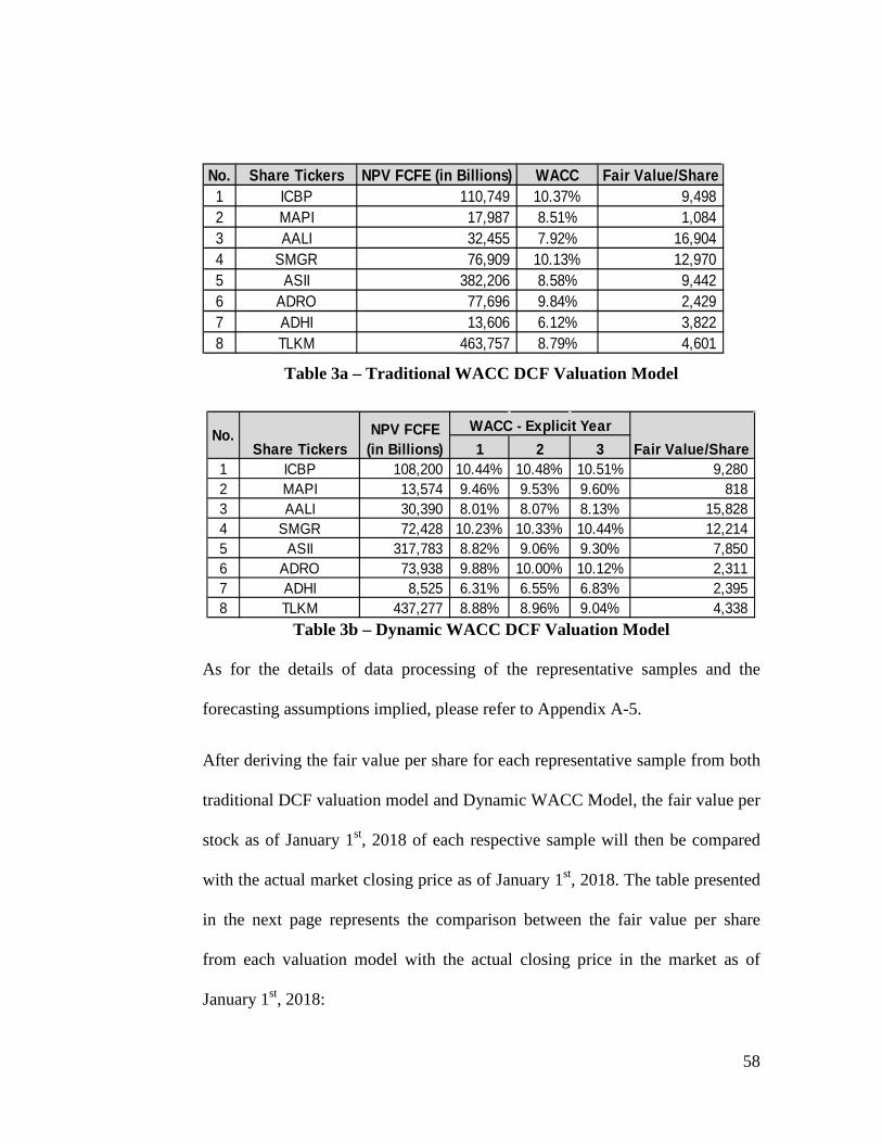
58

No. Share Tickers NPV FCFE (in Billions) WACC Fair Value/Share1 ICBP 110,749 10.37% 9,498 2 MAPI 17,987 8.51% 1,084 3 AALI 32,455 7.92% 16,904 4 SMGR 76,909 10.13% 12,970 5 ASII 382,206 8.58% 9,442 6 ADRO 77,696 9.84% 2,429 7 ADHI 13,606 6.12% 3,822 8 TLKM 463,757 8.79% 4,601

Table 3a – Traditional WACC DCF Valuation Model

1 2 31 ICBP 108,200 10.44% 10.48% 10.51% 9,280 2 MAPI 13,574 9.46% 9.53% 9.60% 818 3 AALI 30,390 8.01% 8.07% 8.13% 15,828 4 SMGR 72,428 10.23% 10.33% 10.44% 12,214 5 ASII 317,783 8.82% 9.06% 9.30% 7,850 6 ADRO 73,938 9.88% 10.00% 10.12% 2,311 7 ADHI 8,525 6.31% 6.55% 6.83% 2,395 8 TLKM 437,277 8.88% 8.96% 9.04% 4,338

WACC - Explicit YearNo.Share Tickers

NPV FCFE (in Billions) Fair Value/Share

Table 3b – Dynamic WACC DCF Valuation Model

As for the details of data processing of the representative samples and the

forecasting assumptions implied, please refer to Appendix A-5.

After deriving the fair value per share for each representative sample from both

traditional DCF valuation model and Dynamic WACC Model, the fair value per

stock as of January 1st, 2018 of each respective sample will then be compared

with the actual market closing price as of January 1st, 2018. The table presented

in the next page represents the comparison between the fair value per share

from each valuation model with the actual closing price in the market as of

January 1st, 2018:

59

No. Share Tickers

Market Price 1 Jan 2018

Traditional Model

1 ICBP 9,275 9,498 2 MAPI 623 1,084 3 AALI 12,950 16,904 4 SMGR 10,900 12,970 5 ASII 8,300 9,442 6 ADRO 1,990 2,429 7 ADHI 1,895 3,822 8 TLKM 4,280 4,601

Table 4a – Traditional WACC Model and Market Price Comparison

No. Share Tickers


Dynamic Model

1 ICBP 9,275 9,280 2 MAPI 623 818 3 AALI 12,950 15,828 4 SMGR 10,900 12,214 5 ASII 8,300 7,850 6 ADRO 1,990 2,311 7 ADHI 1,895 2,395 8 TLKM 4,280 4,338

Table 4b – Dynamic WACC Model and Market Price Comparison

To provide better insights regarding the accuracy and validity of each model in

determining the value of the stock, RMSE statistical analysis will be conducted

to summarize the error of each model in determining the value of each

representative sample. In addition to that, to mitigate the problem of unknown

error distribution, due to the small number of samples, the researcher also

conducted the SE statistical analysis method. Table presented in the next page is

the table representing the error of each model and the implied RMSE and SE:

60

No. Share Tickers


Traditional Model |Error| RMSE SE

1 ICBP 9,275 9,498 223 2 MAPI 623 1,084 461 3 AALI 12,950 16,904 3,954 4 SMGR 10,900 12,970 2,070 5 ASII 8,300 9,442 1,142 6 ADRO 1,990 2,429 439 7 ADHI 1,895 3,822 1,927 8 TLKM 4,280 4,601 321

1,785 1,288

Table 5a – Error in Traditional WACC Model

No. Share Tickers


Dynamic Model |Error| RMSE SE

1 ICBP 9,275 9,280 5 2 MAPI 623 818 195 3 AALI 12,950 15,828 2,878 4 SMGR 10,900 12,214 1,314 5 ASII 8,300 7,850 450 6 ADRO 1,990 2,311 321 7 ADHI 1,895 2,395 500 8 TLKM 4,280 4,338 58

1,151 965

Table 5b – Error in Dynamic WACC Model As for the interpretation of table above, it will be explained in the next section.

4.2. Result and Discussion

4.2.1 Data Interpretation and Theoretical Integration

Based on the data provided in the previous section, the core difference

between the constructed model and the traditional model of DCF valuation

technique is about the determination of the WACC through the forecasted

FCF period (Table 2a and 2b).

61

While the traditional DCF valuation model assumes that the WACC will

remain constant throughout the company’s life, the constructed DCF

model proposed by the researcher takes into account the effect of internal

financing resulted from the retained earnings of the company as explained

in the Pecking Order Theory (Myers, 1984).

To provide better insight regarding the logical reasoning which result in

the different determination of WACC in both valuation models, the

formula of WACC must be revisited. The formula of WACC is as follow:

𝐾𝑐 = (𝐾𝑒 × 𝐸) + (𝐾𝑑 × (1 − 𝐸))

Where Kc= weighted average cost of capital, Ke= cost of equity,

E= weight of equity towards the capital employed, Kd= after-tax cost of

debt, (1-E)= weight of debt towards the capital employed.

The formula of WACC above then can be broken down into two, cost of

equity and cost of debt in which are calculated as follows:

𝐾𝑒 = 𝑅𝑓 + (𝑅𝑚 − 𝑅𝑓) × 𝛽

Where Ke= cost of equity, Rf= risk free, Rm= market risk, β= correlation

for unsystematic risk; and

𝐾𝑑 =𝐼

𝐵𝑉𝐷 × (1 − 𝑇)

62

Where Kd= cost of debt, I= interest expense for the current year,

BVD=book value of debt, and T= effective tax rate.

From the formulas presented above, it is clear that the changes in whether

cost of equity, cost of debt, and the proportion of each financing

instrument will result in the changes of WACC. Therefore, this would be

the main driver in determining the WACC for each model.

To re-enrich the traditional model through integration of internal financing

and Pecking Order Theory, the WACC can be re-stated as follows:

𝐾𝑐 = 𝐾𝑒 ∗ 𝐸𝑛−1 ∗ (1 + 𝑆𝑛)𝑛

𝐷 + 𝐸𝑛−1 ∗ (1 + 𝑆𝑛)𝑛 + 𝐾𝑑 ∗ (1 − 𝑇) ∗ 𝐷

𝐷 + 𝐸𝑛−1 ∗ (1 + 𝑆𝑛)𝑛

In the traditional DCF valuation model, the WACC is assumed at constant

since it implies the irrelevancy of capital structure theory introduced by

Miller and Modigliani (1958) which states that the capital structure of the

company will not affect the cost of the capital of the company in a perfect

capital market. In the proposition, Miller and Modigliani (1958) solved the

equation of cost of equity from the original WACC which is as follow:

𝐾𝑒 = 𝐾𝑐 + (𝐾𝑐 − 𝐾𝑑) ×𝐷𝐸

The formula above implies that any efforts to change the proportion of the

financing sources to a cheaper one (which is debt) will result in the

63

increasing perception of risk regarding the remaining equity holders in

which the increase is just about equivalent to offset the effect of lowering

the WACC through increasing weight of debt and therefore, the WACC

will remain constant and the financing options will not affect the WACC

at all.

However, there are some critics regarding this theory. As mentioned by

Myers (2001), should the Miller and Modigliani is acceptable in the real

finance practice, there must be no financing strategy required for the

companies to survive in the industry, while in fact there are so many

financial innovations conducted by the Chief Financial Officer (“CFO”) of

the companies to achieve the optimal capital structure of the company.

In regards to the critics of Miller and Modigliani (1958), there are some

capital structure theories developed such as tradeoff theory, free cash flow

theory, and pecking order theory as what have been mentioned in the

literature review.

The difference of the constructed model with the traditional model of DCF

valuation lies in terms of the consideration of internal financing impact to

the perception of the investors and the WACC of the company. In align

with the suggestion from Koller et al (2010) which suggests that any

corporate actions such as debt issuance, of equity issuance shall be

assumed constant due to its unavailability of the forecasting, the

64

constructed model offered the dynamics or changing of WACC through

the changing in internal financing capacity.

According to the Pecking Order Theory, the company will try to finance

its operations by using the safest financial resources first that is the

internal financing since it is considered as the “cheapest” financing

sources of the companies in which they don’t need to incur additional

costs to raise the funds for the operation’s financing. The internal

financing is derived from the company’s retained earnings, generated from

the operations of the current year and therefore will become part of the

equity proportion in the capital structure.

As what can be seen in Table 2a and 2b, the dynamic WACC model

provides higher WACC than the traditional model. This is caused by the

increasing of retained earnings in the company which then increases the

proportion of equity towards the capital employed. According to Berk et al

(2015), there is a dimension in cost of capital called the cost of retained

earnings which is formulated exactly the same as the cost of common

equity. The philosophy behind the cost of retained earnings is the lost

opportunity for the investors who reinvest the earnings back to the

business rather than withdrawing the earnings in form of dividends

income and therefore expects a certain amount of return based from the

investment. This philosophy is align with the cost of common equity in

65

which the return expectation is derived from the perception of the risk

towards the company that the equity investors are investing in. In this

study, the combination of both common equity and retained earnings will

be referred as the “cost of equity”.

Therefore, based on the aforementioned premises and theories, the

dynamic WACC model provides better framework and understanding in

valuing the fair value of company’s stock in some dimensions.

The dynamic WACC is capable to explain and integrate the impact of

internal financing to the changes in capital mix and therefore, the value of

the company compared with the traditional model which assumes that the

capital mix are at constant rate. The weakness of implying the traditional

model is that the company is assumed to issue debt over time along with

the increase of the company’s performance without considering the

utilizations of the new issued debts to the operation of the company.

In addition to that, by emphasizing on the internal capacity of the

company to grow its own equity and assuming constant level of debt, this

dynamic WACC model implies that the “real value” of the company is

resulted from the operations of the company and its capacity to reinvest

those internal funds to expand the operation of the company. This

implication covers the weakness of free cash flow and irrelevant theories

which imply that the value of the company can be affected by the increase

66

of leverage. Even though integrating the effect of financial leverage will

provide more insights regarding the company’s fair value, however, from

the perspective of the equity holders, the ability to internally grow over

the time will be the best indicator to identify worth-investing company.

The last advantage of the dynamic WACC model is the focus on present

condition of financial leverage without overweighing the impact of

financial leverage in the future. Unlike traditional model which assumes

new debt issuance over the explicit forecast period or future, the dynamic

WACC model focuses on finding the true value “at the present time” by

subtracting the current level of debt from the firm’s value to derive the

share’s fair value. This concept was in align with the suggestion of Koller

et al (2010) which states that matching the cost of equity with real cash

flow stream for the equity is not feasible unless the company’s capital mix

is 100% equity.

4.2.2 Data Validation Result through Quantitative Approach

Based on what have been explained in the previous section, the Dynamic

WACC model proposed by the researcher possesses conceptual

advantages over the traditional WACC model. In addition to the

67

conceptual advantages, the researcher had tested the validity of the

Dynamic WACC model through the quantitative approach as well.

It can be seen from the table 4a and 4b provided in the data description

section that the Root Mean Squared Error (RMSE) of the traditional

WACC model is 1,785 while the RMSE of the Dynamic WACC model is

1,151. It should be noted that in the quantitative testing, both of the

Traditional and Dynamic WACC models are tested against the same

market prices of each representative sample. All of the variables in both

models are kept constant except the WACC variable.

Recalling that RMSE indicates the error resulted by the estimators (“in

this research, the model”) in predicting the actual output (Chai and

Draxler, 2014), higher RMSE indicates higher error of one model in

predicting the actual output and vice versa. Therefore, it can be concluded

that the higher RMSE of Traditional WACC model which is 1,785

indicates lower accuracy of the model compared with Dynamic WACC

model which is 1,151.

The researcher is aware that the figure represented by the RMSE in the

Dynamic WACC model is highly influenced by the number of

representative samples taken and the distribution of each data point in the

representative samples. The distribution of the market price of each

representative sample as of January 1st, 2018 can be seen in Table 2.

68

From the Box-Plot provided in Figure 1, the data from representative

samples are widely distributed. This could result in the biased RMSE

interpretation of each representative sample. Though the MAD

preliminary filtering has been done, it can only mitigate the bias of market

over-confidence towards certain share compared with the industry

performance. However, mitigating the mean bias of cross-sectional data

from representative sample is not feasible, especially in case of small

sample scope.

Though RMSE has provided insight regarding the accuracy of the model,

to provide more valid accuracy interpretation, the researcher utilizes the

SE statistical analysis as well. Based on the data presented in Table 4a and

4b, the Traditional WACC model possesses SE of 1,288 while the

Dynamic WACC possesses SE of 965. While RMSE indicator shows the

mean error of an estimator towards actual data set, the SE indicator adjust

the error by comparing each error with the average of errors implied by

the estimator.

In nature, SE indicates the same measurement of error with RMSE and it

is interpreted the same way with RMSE. The SE of Traditional WACC

model is higher than the Dynamic WACC model which indicates that the

Dynamic WACC model proposed by the researcher is still more accurate

compared with the Traditional WACC model. The reduction of 323 in SE

69

indicator can be interpreted as the increase of accuracy in Dynamic

WACC model compared with the Traditional WACC model.

Based on the validation of both qualitative and quantitative approaches, it

can be seen that the Dynamic WACC model provides better conceptual

advantages and accuracy in determining the fair value of company’s share

price both from RMSE and SE indicators.

70

CHAPTER V:

CONCLUSION AND RECOMMENDATION

5.1. Conclusion

The purpose of this study is to construct new DCF valuation model which

integrates the internal financing impact on the capital structure of the company

through theoretical integration and provides sufficient evidence regarding the

validity and accuracy of the model through quantitative approach.

By using the MAD as the filtering process in sampling design and random

stratified sampling, the researcher obtained eight companies to be then used as

the representative samples of each industry sector in JASICA. Free cash flows

of each representative samples then were forecasted by using the financial

information from the prior year as basis. The fair value estimation results of the

new DCF valuation model and the traditional model thus were compared to the

actual market price as of January 1st, 2018 and analyzed by using RMSE and SE

to mitigate the impact of small number of samples.

Based on the statistical analysis RMSE and SE that are presented in the

previous section, it can be concluded that the constructed model proposed by

the researcher provides better accuracy in determining the fair value of the

company and thus more reliable in determining the market price expectation

71

compared with the traditional model since RMSE and SE of Dynamic WACC

model is lower compared with the Traditional WACC model.

5.2. Limitations and Recommendations

5.2.1 Limitations of Dynamic WACC Model

As what has been mentioned in the literature review, every valuation

technique provides different approach and assumptions in estimating the

fair value of an asset. Thus, the fair value resulted from each model is

limited to the approach and assumptions implied in the model.

In the Dynamic WACC model constructed by the researcher, the model

implies that the debt level of a company is assumed at constant due to the

suggestion of Koller et al (2010) which suggested that the corporate

actions such as issuance of debt and equity are not feasible to be predicted.

The Dynamic WACC model implies that the “dynamic” aspect of the

WACC is resulted solely due to the increase of internal financing

(Retained Earnings) which is generated as the operation’s result. Since the

Retained Earnings changed the equity proportion towards the capital

employed, therefore, the WACC is increased along with the forecast

periods. In addition to that, the model also applies optimistic approach in

the FCF forecasting since this was in align with Walther and Willis (2013)

72

which stated that the analysts’ forecast commonly is very optimistic due to

the impact of investors’ expectations towards the company. The Dynamic

WACC model doesn’t cover the financial industry sector in JASICA due

to the difference of valuation framework and business operations

compared with the non-financial industry.

5.2.2 Recommendations for Future Research

Though the assumptions in Dynamic WACC model may provide

advantages from the perspective of practical dimension, there are still so

many opportunities for the future researches to develop other valuation

model.

Future research may integrate other dimensions which affect the WACC.

The research of Vélez-Pareja et al (2008) integrated the Tradeoff Theory

which focuses on the changes of leverage level due to the impact of tax

shield generated by the debt financing, while the model constructed by the

researcher integrates the Pecking Order Theory which focuses on the

changes of internal financing capacities which affect the equity proportion

towards the company.

In addition to that, future research may focus on the development of the

valuation of financial institutions. As what the researcher had been

73

observed during the literature review, most of the researches conducted in

valuation subject are more focused on the non-financial industry rather

than the financial industry. This could become an opportunity for the

future research.

According to Lundholm (2001), the research in valuation subjects should

not focus only on comparing the existing models, but also focuses on

increasing the accuracy of the valuation. This suggestion therefore may be

very useful for the framework in the future research.

The last dimension that the researcher can offer for the future researcher

would be about the observation in the other dimension in the DCF

valuation model, such as periods and terminal value.

5.3. Implications

The researcher believes that the Dynamic WACC model constructed by the

researcher is suited for the current practical condition of finance field. The

implementation of this Dynamic WACC model can provide advantages as

follow:

a. Better and more reliable discount factor by taking into account the

increasing of investors’ demand towards the company’s internal financing

74

sources. This framework was aligned with the literatures of Berk et al

(2015).

b. Capability to integrate the internal financing capacity as the valuation

framework. This model emphasizes the importance of the company to self-

develop themselves through the retained earnings of the company. Unlike

the Free Cash Flows Theory which implies that the excessive financial

leverage will provide value for the company;

c. By expressing the equity value as the firm value deducted by the net debt

value, the model provides better methodology in matching the free cash

flows with the respective discount factor.

By implementing the Dynamic WACC model, the sell-side analysts could

provide better target price which integrates the real increase of market’s

expectation towards certain company’s share while also focusing on the internal

capacity of the company to grow rather than misleadingly taken into the account

the excessive amount of leverage as the efforts to increase shareholders’ value.

By focusing on this internal capacity of the firm to grow over time, the Merger

and Acquisition analysis can also be benefited. The bidder firm can avoid the

unfavorable MnA deal due to the extreme optimistic synergy valuation since the

Dynamic WACC model provides “adjustment” towards the optimistic valuation.

Therefore, the researcher suggests that the implementation of Dynamic WACC

constructed by the researcher will provide better insights and framework in the

75

valuation and better accuracy compared with the traditional DCF valuation

model.

APPENDIX

A-1) Growth Domestic Product (GDP) of Indonesia 2011-2018

Year GDP Growth (Y-o-Y)2013 5.56%2014 5.01%2015 4.88%2016 5.03%2017 5.07%

004%

005%

005%

005%

005%

005%

006%

006%

2013 2014 2015 2016 2017

GDP Growth (Y-o-Y)

76

A-2) Increase of Bank Indonesia 7-Days Repo Rate

77

A-3) Risk-Free Rate: PBS014 (Yield:6.89%, TTM:2.34)

78

A-4) Price-Earning (P/E) and Median Absolute Deviation (MAD)

83

A-3) Financial Statements, Forecast, and Assumptions

a. PT Indofood CBP Sukses Makmur, Tbk.

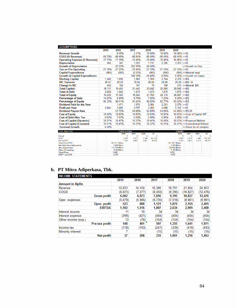
84

b. PT Mitra Adiperkasa, Tbk.

86

c. PT Astra Agro Lestari, Tbk.

88

d. PT Semen Indonesia (Persero), Tbk.

90

e. PT Astra International, Tbk.

92

f. PT Adaro Energy, Tbk.

94

g. PT Adhi Karya (Persero), Tbk.

96

h. PT Telekomunikasi Indonesia (Persero), Tbk.

98

REFERENCES

Aselage, J., & Eisenberger, R. (2003). Perceived organizational support and psychological contracts: a theoretical integration. Journal of Organizational Behavior, 491-509.

Baskin, J. (1989). An Empirical Investigation of the Pecking Order Hypothesis. Financial Management 18 (1), 26-35.

BasuS. (1975). The Information Content of Price-Earnings Ratios . Financial Management, 4(2), 53-64.

Berk, J., DeMarzo, P., & Harford, J. (2015). Fundamentals of Corporate Finance, Global Edition. Pearson.

Burmeister, E., & Aitken, L. (2012). Sample size: How many is enough? Australian Critical Care 25 (4), 271-274.

Chai, T., & Draxler, R. (2014). Root mean square error (RMSE) or mean absolute error (MAE)?- Arguments against avoiding RMSE in the literature. Geoscientific model development, 7(3), 1247-1250.

Chen, L., & Chen, S. (2011). How the Pecking Order Theory Explain Capital Structure. Journal of International Management STudies 6 (3), 92-100.

Chen, S., & Dodd, J. (1997). Economic Value Added (EVA): An Empirical Examinaion of a New Corporate Performance Measure. Journal of Managerial Issues, 318-333.

Courteau, L., Kao, J., & Richardson, G. (2000). The equivalence of dividend, cash flows and residual earnings approaches to equity valuation employing ideal terminal value expression. Working paper, Université Laval.

Damodaran, A. (2012). Investment Valuation: Tools and Techniques for Determining the Value of Any Asset, 3rd ed. New Jersey: John Wiley & Sons.

Fazzini, M. (2018). Business Valuation: Theory and Practice. Springer.

Fernández, P. (2007). Company Valuation Methods. The Most Common Errors in Valuations. IESE Working Paper No. 449. .

Francis, J., Olsson, P., & Oswald., D. (2000). Comparing the accuracy and explainability of dividend, free cash flow and abnormal earnings equity value estimation. Journal of Accounting Research (38), 45-70.

99

Givoly, D., Hayn, C., & Lehavy, R. (2009). The Quality of Analysts' Cash Flow Forecasts. The Accounting Review 84 (6), 1877-1911.

Hair, J., Black, W., Babin, B., & Anderson, R. (2010). Multivariate Data Analysis. Pearson.

IAS Plus. (2019, January 5). Conceptual Framework for Financial Reporting 2018. Retrieved from Conceptual Framework for Financial Reporting 2018: www.iasplus.com/en/standards/other/framework

Ikatan Akuntan Indonesia. (2019, January 5). PSAK 68 Pengukuran Nilai Wajar - Ikatan Akuntan Indonesia. Retrieved from PSAK 68 Pengukuran Nilai Wajar - Ikatan Akuntan Indonesia: iaiglobal.or.id/v03/standar-akuntansi-keuangan/pernyataan-sak-56-psak-68

Indonesia Bond Pricing Agency. (2019, January 5). Indonesia Bond Pricing Agency. Retrieved from Indonesia Bond Pricing Agency: www.ibpa.co.id/DataPasarSuratUtang/BondMaster/ObligasidanSukukPemerintah/tabid/79/Default.aspx

Indonesia, S. B. (2019, January 5). Biro Pusat Statistik. Retrieved from Biro Pusat Statistik: https://www.bps.go.id/subject/11/produk-domestik-bruto-lapangan-usaha-.html

Jason, L., & Glenwick, D. (2016). Handbook of Methodological Approaches to Community Based Research. New York: Oxford University Press.

Jennergren, L. (2008). Continuing value in firm valuation by the discounted cash flow model. European Journal of Operational Research, 185, 1548-1563.

Kementrian Keuangan Republik Indonesia Badan Pengawas Pasar Modal dan Lembaga Keuangan. (2012, June 25). Penyajian dan Pengungkapan Laporan Keuangan Emiten atau Perusahaan Publik. Jakarta, Jakarta, Indonesia.

Koller, T., Goedhart, M., & Wessels, D. (2010). Valuation: Measuring and Managing the Value of Companies, 5th Edition. New Jersey: John Wiley & Sons.

Leys, C., Ley, C., Klein, O., Bernard, P., & Licata, L. (2013). Detecting outliers: Do not use standard deviation around the mean, use absolute deviation around the median. Journal of Experimental Social Psychology, 49(4), 764-766.

Lobo, G. (1992). Analysis and comparison of financial analysts', time series, and combined forecasts of annual earnings. Journal of Business Research 24 (3), 269-280.

100

Merton, R. (1976). Option pricing when underlying stock returns are discontinuous. Journal of Financial Economics, 125-144.

Modigliani, & Miller. (1958). The Cost of Capital, Corporation Finance and Theory of Investment. The American Economic Review, 48 (3), 261-297.

Myers, S. (1984). The Capital Structure Puzzle. Journal of Finance 39, 575-592.

Myers, S. (2001). Capital Structure. Journal of Economic Perspectives, 15 (2), 81-102.

Noor, T., Sinaga, B., & Maulana TB, N. (2015). Testing on Pecking Order Theory and Analysis of Company's Characteristic Effects on Emitten's Capital Structure. Indonesian Journal of Business & Entrepreneurship 1 (2), 81-89.

Parker, R. (1968). Discounted Cash Flow in Historical Perspective. Journal of Accounting Research, 58-71.

Penman, S., & Sougiannis, T. (1998). A comparison of dividend, cash flow, and earnings approaches to equity valuation. Contemporary Accounting Research 15 (Fall), 343-383.

Ross, S. W. (2015). Corporate Finance Asia Global Edition. Singapore: McGraw-Hill Education (Asia).

Rosso, B., Dekas, K., & Wrzesniewski, A. (2010). On the meaning of work: A theoretical integration and review. Research in Organizational Behavior, 91-127.

Rousseeuw, P., & Croux, C. (1993). Alternatives to the median absolute deviation. Jounral of the American Statistical Association, 88(424, 1273-1283.

Sayed, S. (2017). How much does valuation model choice matter? Target price accuracy of PE and DCF model in Asian emerging markets. Journal of Accounting in Emerging Economies, 7(1), 90-107.

Seale, C. (1999). Quality in qualitative research. Qualitative Inquiry 5(4), 465-478.

Sekaran, U., & Bougie, R. (2016). Research Methods for Business. West Sussex: John Wiley & Sons.

Statistic Bureau of Indonesia. (2019, January 5). Badan Pusat Statistik. Retrieved from Badan Pusat Statistik: bps.go.id/subject/11/produk-domestik-bruto-lapangan-usaha-.html

101

Vélez–Pareja, I., Ibragimov, R., & Tham, J. (2008). Constant Leverage and Constant Cost of Capital : A Common Knowledge Half-Truth. Estudios Gerenciales, 24(107), 13-33.

Vogt, S. (1994). The role of internal financial sources in firm financing and investment decisions. Review of Financial Economics, 1-24.

Walther, B., & Willis, R. (2013). Do investor expectations affect sell-side analysts' forecast bias and forecast accuracy? Review of Accounting Studies, 207-227.

Weygandt, J., Kimmel, P., & Kieso, D. (2012). Financial Accounting, IFRS Edition, 2nd Edition. Wiley Textbook.

Wiggins, B. (2011). Confronting the dilemma of mixed methods. Theoretical and Philisophical Psychology 31, 44-60.

Yulianto, A., Suseno, D., & Widiyanto. (2016). Testing Pecking Order Theory and trade Off Theory Models in Public Companies in Indonesia. International Journal of Economic Perspectives 10 (4), 21-28.

dynamic wacc: re-enrichment of discounted cash flow

Documents