dynamic van der waals theory - 京都大学理学研...

Dynamic van der Waals theory

Akira OnukiDepartment of Physics, Kyoto University, Kyoto 606-8502, Japan

�Received 26 October 2006; published 9 March 2007�

We present a dynamic van der Waals theory starting with entropy and energy functional with gradientcontributions. The resultant hydrodynamic equations contain the stress arising from the density gradient. Itprovides a general scheme of two-phase hydrodynamics involving the gas-liquid transition in nonuniformtemperature. Some complex hydrodynamic processes with evaporation and condensation are examined numeri-cally. They are �i� adiabatically induced spinodal decomposition, �ii� piston effect with a bubble in liquid, �iii�temperature and velocity profiles around a droplet in heat flow, �iv� efficient latent heat transport at small liquiddensities �the mechanism of heat pipes�, �v� boiling in gravity with continuous bubble formation and rising, and�vi� spreading and evaporation of liquid on a heated boundary wall.

DOI: 10.1103/PhysRevE.75.036304 PACS number�s�: 47.20.Dr, 05.70.Ln, 64.70.Fx, 44.35.�c

I. INTRODUCTION

The van der Waals theory provides a simple description ofgas-liquid phase transitions in one-component fluids �1�. It isan equilibrium mean-field theory for hard sphere particleswith long-range attractive interaction �2�. Moreover, in hispioneering paper in 1893, van der Waals introduced a gradi-ent term in the Helmholtz free energy density to describe agas-liquid interface. Such a gradient term began to be widelyused in statistical mechanics of nonuniform states, sinceseminal papers by Ginzburg and Landau for type-I supercon-ductors �3� and by Cahn and Hilliard for binary alloys �4�.

In most phase transition theories, including those of dy-namics, the temperature T is a given parameter independentof space �5,6�. The Ginzburg-Landau theory is based on afree energy functional with homogeneous T. It goes withoutsaying that there are a variety of situations, where phasetransitions occur in inhomogeneous T or in heat flow. In fluidsystems, wetting dynamics �7–11�, boiling processes�12–14�, and droplet motion �15,16� are strongly influencedby applied heat flux. Rayleigh-Bénard convection is verycomplex in liquid crystals with first-order phase transition�17� and in binary fluid mixtures with phase separation�18–20�. In He4, the superfluid transition can be nonlinearlyinfluenced by heat flux, where a sharp interface is producedseparating superfluid and normal fluid �21,22�. Understand-ing such a problem is very difficult. We need to construct adynamical model first to study nonequilibrium effects, wherephase transitions and hydrodynamics are inseparablycoupled.

In 1901, Korteweg proposed hydrodynamic equations forbinary fluid mixtures including the stress induced by compo-sition gradients �23�. Diffuse interfaces between two-phasesthen arise in solutions of the hydrodynamic equations in thepresence of the gradient stress �24–26�. In this line, a numberof two-dimensional simulations of diffuse-interface modelshave been presented to describe two-phase hydrodynamics inone-component fluids �6,14� and in binary mixtures�19,20,26–28�. One-dimensional numerical solutions arethemselves highly nontrivial in heat flow �29,30�. Note thatdiffuse-interface models or phase field models have beenused in numerical analysis of dendrite instability in crystal

growth �31–33�. As another line of research, critical dynam-ics in classical fluids was studied with inclusion of the gra-dient contributions of the mass density and the composition,which are relevant even in one-phase states with growing ofthe correlation length near the critical point �5,6,34–38�. Theso-called model H for near-critical binary mixtures wasoriginally devised to describe dynamics of the thermal fluc-tuations �5�, but has also been used to describe phase sepa-ration processes �39� and steady states under shear flow�6,40�. We mention Kawasaki’s hydrodynamic equations forvan der Waals fluids with long-range interaction �36�, wherethe stress is of a nonlocal convolution form but reduces tothe well-known form in critical dynamics in the gradientapproximation �41�. For He4, on the other hand, a set ofnonlinear hydrodynamic equations with the gradient contri-butions was established in an early period �42�, whose sim-plified version near the superfluid transition was later used incritical dynamics �5,6� and in studying nonlinear effects ofheat flow �21�.

Recently, we presented a dynamic van der Waals theoryon the basis of entropy and energy functionals containing thegradient contributions �15�. We then constructed hydrody-namic equations with the gradient stress and numericallysolved them to examine droplet motion in heat flow. One ofour findings is that the temperature becomes homogeneouswithin a droplet under applied heat flux without gravity. La-tent heat transport is so efficient such that the interface re-gion is nearly on the coexistence curve T=Tcx�p� even innonequilibrium, where the pressure p is uniform outside thedroplet. This picture was confirmed in a subsequent hydro-dynamic theory �16�. As a result, the Marangoni effect aris-ing from inhomogeneous surface tension is not operative inone-component �pure� fluids, while it gives rise to muchfaster fluid and interface motions in mixtures even at verysmall impurity concentrations �43�.

In this paper, we will present a general scheme of thedynamic van der Waals theory in one-component fluids in ageneral form and give numerical results of some fundamen-tal but complicated processes with evaporation and conden-sation. Section II will be a theoretical part, while Sec. III willpresent some numerical illustrations of such processes.

PHYSICAL REVIEW E 75, 036304 �2007�

1539-3755/2007/75�3�/036304�15� ©2007 The American Physical Society036304-1

http://dx.doi.org/10.1103/PhysRevE.75.036304

II. THEORY

A. van der Waals theory

We summarize the main results of the van der Waalstheory �1,6�, which will be needed in constructing our theory.As a function of the number density n and the temperature T,the Helmholtz free density f�n ,T� for monoatomic moleculesis written as

f = kBTn�ln��thd n� − 1 − ln�1 − v0n�� − �v0n2, �2.1�

where v0=ad is the molecular volume and � is the magnitudeof the attractive potential with d being the space dimension-ality. The molecular radius is given by a=v0

1/d. The �th=��2� /mT�1/2 is the thermal de Broglie length with m beingthe molecular mass. As functions of n and T, the internalenergy density e, the entropy s per particle, and the pressurep are given by �44�

e = dnkBT/2 − �v0n2, �2.2�

s = − kB ln��thd n/�1 − v0n�� + kB�d + 2�/2, �2.3�

p = nkBT/�1 − v0n� − �v0n2. �2.4�

In this paper, use will be made of the expressions for thesound velocity c= ��p /�n�s /m�1/2 and the specific heat ratio�s=Cp /CV,

c = �kBT/m�1/2�1 + 2/d − Ts/T�1/2, �2.5�

�s = 1 + 2/d�1 − Ts/T� . �2.6�

where CV=dnkB /2 is the constant-volume specific heat andCp is the isobaric specific heat per volume. We introduce thespinodal temperature,

Ts = 2�v0n�1 − v0n�2/kB. �2.7�

Maximization of Ts�n� as a function of n yields the criticaltemperature Tc=8� /27kB and the critical density nc=1/3v0.

As mentioned in Introduction, van der Waals introducedthe gradient free energy density,

fgra =1

2M��n�2, �2.8�

We consider the equilibrium interface density profile n=n�x� varying along the x axis. The chemical potential perparticle ��n ,T�= ��f /�n�T changes as

� − �cx =M

2

d2n

dx2 +d

dx

M

2

dn

dx, �2.9�

where �cx�T� is the chemical potential on the coexistencecurve. From dp=nd� at constant T, the van der Waals pres-sure p�n ,T� in Eq. �2.4� is expressed as �6�

p − pcx =M

2n

d2n

dx2 +d

dx

M

2n

dn

dx− M�dn

dx�2

, �2.10�

where pcx�T� is the the pressure on the coexistence curve. InSec. II D, a stress tensor �ij including gradient contributionswill be introduced, in terms of which Eq. �2.10� is equivalent

to �xx= pcx �see discussions below Eq. �2.50��. The surfacetension ��T� is expressed as �6,45,46�

� = �−

dxM�dn/dx�2. �2.11�

We note that Eqs. �2.9�–�2.11� hold even if M depends on nas M =M�n� �while M was a constant in the original theory�1��.

B. Gradient entropy and energy

We generalize the van der Waals theory by including gra-dient contributions to the entropy and the internal energy as

Sb =� drns�n,e� −1

2C��n�2 , �2.12�

Eb =� dre +1

2K��n�2 , �2.13�

where the space integrals are within the container of thefluid. The entropy and energy contributions at the boundarywalls will be introduced in Eq. �2.28� below. The entropydensity and the internal energy density including the gradientcontributions are thus written as

S = ns −1

2C��n�2, �2.14�

e = e +1

2K��n�2. �2.15�

The gradient terms represent a decrease of the entropy and anincrease of the energy due to inhomogeneity of n. They areparticularly important in the interface region. For simplicity,we neglect the gradient terms proportional to ��n� ·�e and��e�2. The gravitational energy is also neglected, but its in-clusion is trivial �see discussions around Eq. �2.51��. In thiswork, in constructing a general theory, we allow that C andK depend on n as

C = C�n�, K = K�n� . �2.16�

However, in our simulations in the next section, we will setK=0 and assume that C is independent of n.

We then define the local temperature T=T�n ,e� by

1

T= �

eSb�

n= n� �s

�e�

n, �2.17�

where n is fixed in the derivatives. This definition of T isanalogous to that in a microcanonical ensemble. We will useit even for inhomogeneous n and e in nonequilibrium. Wealso define a generalized chemical potential � per particleincluding the gradient contributions by

� = − T�Sb

n�

e= � − T � ·

M

T� n +

M�

2��n�2,

�2.18�

where the internal energy density e in Eq. �2.15� is fixed sowe set e=−�K��n�2 /2� in the functional derivative. The

AKIRA ONUKI PHYSICAL REVIEW E 75, 036304 �2007�

036304-2

�= �e+ p� /n−Ts is the usual chemical potential per particleand

M = CT + K . �2.19�

Obviously, M is the coefficient of the gradient term in theHelmholtz free energy defined in equilibrium �see the nextsection�. Under Eq. �2.16�, M =M�n ,T� depends on n and T,so M�= ��M /�n�T in Eq. �2.18� is its derivative with respectto n. Now, regarding Sb as a functional of n and e, we con-sider small changes n and e of n and e which yield anincremental change of Sb. Using Eq. �2.18� and e=e−�K��n�2 /2�, we obtain

Sb =� dr� 1

Te −

�

Tn� −� da

M

T�� · �n�n .

�2.20�

The second term is the surface integral, where da is thesurface element and � is the outward normal unit vector atthe surface.

We remark on the following two papers. Fixman proposedthe energy and entropy functionals, but without the gradiententropy, to calculate the transport coefficients near the criti-cal point �34�. Anderson et al. started with energy and en-tropy functionals to include the velocity field in the solidifi-cation problem �33�.

C. Equilibrium conditions

In equilibrium, we maximize Sb at a fixed particle numberN=�drn and a fixed energy Eb=�dr� for a fluid confined ina cell. First, we are interested in the bulk equilibrium. To thisend, we introduce

W = Sb/kB + �N − �Eb, �2.21�

where � and � are the Lagrange multipliers. The maximiza-tion condition �W /e�n=0 with respect to e at fixed n yieldsthe homogeneity of the temperature,

T = 1/kB� �2.22�

and then

W = �− F + kBT�N�/kBT �2.23�

becomes a functional of n. We introduce the Helmholtz freeenergy functional,

F = Eb − TSb =� dr� f�n,T� +M

2��n�2� , �2.24�

where the integrand is e−TS, so f =e−Tns and M is definedby Eq. �2.19�. In the Ginzburg-Landau theory, we further-more minimize W with respect to n to obtain

� = kBT� = const, �2.25�

where � is defined by Eq. �2.18�. In the thermodynamic limitwe find W= pV /kBT where p is the pressure and V is the totalvolume of the fluid.

In a two-phase state with a planar interface at x�0, thesurface tension � is expressed as Eq. �2.11�. Here we intro-duce the grand potential density,

g�n,T� = f�n,T� − �cxn + pcx, �2.26�

where �cx and pcx are the values of � and p on the coexist-ence curve. It is nonvanishing in the interface region, wheren=n�x� changes from a gas density ng to a liquid density n�

as a function of x. From Eq. �2.25� it holds the relationg�n ,T�=M�dn /dx�2 /2 and

��T� = �ng

n�

dn�2Mg�n,T��1/2. �2.27�

This expression holds even when M depends on n �6�.In real fluids we need to consider the boundary condition

on the surface of the container. For simplicity, we considerthe surface entropy and energy of the forms,

Ss =� da s�n�, Es =� daes�n� , �2.28�

where da is the surface element and the areal densities sand es are assumed to depend only on the number density non the surface. We need to maximize the total entropy Stot=Sb+Ss under fixed N and Etot=Eb+Es. To this end, we in-troduce

Wtot = W +� da� s − �es� , �2.29�

where � is common to that in Eq. �2.22�. Maximization ofthe surface part of Wtot additionally yields

M� · �n + ��fs/�n�T = 0, �2.30�

as the surface boundary condition. Here we use Eq. �2.20�and define the Helmholtz surface free energy density,

fs�n,T� = es − T s. �2.31�

In equilibrium, the temperature is homogeneous and weshould minimize the total Helmholtz free energy,

Ftot = F +� dafs�n,T� , �2.32�

in order to calculate the surface density profile �7,48�. Thesurface free energy is usually expanded to second order inn−nc as

fs = − as�n − nc� + bs�n − nc�2/2, �2.33�

where as and bs are constants. Then the boundary condition�2.30� is written as

M� · �n − as + bs�n − nc� = 0. �2.34�

D. Generalized hydrodynamic equations

We propose hydrodynamic equations taking account ofthe gradient entropy and energy. They are of the same formsas those of compressible fluids in the literature �47� exceptthat the stress tensor contains gradient contributions. Theguiding principle of their derivation is the non-negative defi-niteness of the entropy production rate in the bulk region. Inthe previous theories �24,26,28� the gradient entropy was not

DYNAMIC VAN DER WAALS THEORY PHYSICAL REVIEW E 75, 036304 �2007�

036304-3

assumed and M =K in Eq. �2.19�. We suppose that a fluid isin a solid container with controllable boundary temperaturesand the velocity field v vanishes on the boundary. We here-after include a gravity g applied in the downward directionalong the z axis.

First, the number density n obeys

�n

�t= − � · �nv� . �2.35�

The mass density is defined by �=mn, where m is the par-ticle mass. Second, the momentum density �v obeys

�

�t�v = − � · ��vv� − � · ��J − J� − �gez, �2.36�

where the last term arises from the gravity with ez being the

�upward� unit vector along the z axis. The �J = �ij� is thereversible stress tensor containing the gradient contributions,which is invariant with respect to time reversal v→−v. The J= ij� is the dissipative stress tensor of the form,

ij = ��iv j + � jvi� + �� − 2�/d�ij � · v �2.37�

with �i=� /�xi. The � and � are the shear and bulk viscosi-ties, respectively. Third, including the kinetic part, we definethe �total� energy density,

eT = e + �v2/2. �2.38�

We assume that the energy current is of the usual form in

terms of the stress tensor �J − J and the thermal conductivity�. Then eT is governed by �47�

�

�teT = − � · �eTv + ��J − J� · v� + � · �� T� − g�vz.

�2.39�

Equivalently, we may rewrite the above energy equation interms of the internal energy density e using Eqs. �2.35� and�2.36� as

�

�te = − � · �ev� −�J :�v + �v + � · �� T� , �2.40�

where there is no term proportional to g. On the right-handside of Eq. �2.40�, the second term represents −�ij�ij�iv jand �v=�ij ij�iv j is the viscous heat production rate. Use ofEq. �2.37� gives

�v = �ij

�

2��iv j + � jvi −

2

dij � · v�2

+ �� · v�2 � 0.

�2.41�

From Eq. �2.20� the time derivative of Sb becomes com-posed of bulk and surface contributions as

dSb

dt=� dr� 1

T

�e

�t−�

T

�n

�t� −� da�� · �n�

M

T

�n

�t.

�2.42�

From our hydrodynamic equations the first bulk term be-comes

�dSb

dt�

bulk=� drv · �� ·

�J

T+ e �

1

T− n �

�

T�

+1

T�� · � � T + �v� . �2.43�

If there is no heat flow from outside, the above quantityshould be non-negative definite. We thus require

�j

� j� 1

T�ij� = − e�i

1

T+ n�i

�

T. �2.44�

Under Eq. �2.44� we obtain �dSb /dt�bulk=�dr��v+ �� /T�0without heat input from the boundary �47�, where the ther-mal heat production rate is

�� = ��T�2/T� 0. �2.45�

Now we seek the symmetric tensor �ij which satisfies Eq.�2.44�. Notice the thermodynamic identity,

d�p/T� = − ed�1/T� + nd��/T� , �2.46�

following from the Gibbs-Duhem relation d�=−sdT+dp /n�6�, where d�¯� denotes an infinitesimal change. If the gra-dient stress is neglected, we have �ij = pij, as should be thecase, where p= p�n ,T� is the van der Waals pressure in Eq.�2.4�. If it is included, some calculations yield

�ij = �p + p1�ij + M��in�� jn� , �2.47�

where p1 is a diagonal gradient part,

p1 = �nM� − M��n�2

2− Mn�2n − Tn��n� · �

M

T

= n� − e + TS − p . �2.48�

In the first line of Eq. �2.48�, the last term does not exist inthe previous theories �26�. The second line indicates that Eq.�2.48� is a generalization of the thermodynamic identity p=n�−e−Tns. In Appendix A, we will present another deri-

vation of the above expression for �J using Eqs. �2.35� and

�2.40�. With the above form of �J , the total entropy density Sin Eq. �2.14� obeys

�

�tS = − � · Sv −

M

Tn�� · v� � n −

�

T� T + ��v + ��/T .

�2.49�

The additional entropy flux −T−1Mn�� ·v��n is reversibleand is nonexistent in the usual hydrodynamics �47�. The lastterm on the right-hand side is the usual entropy productionrate per unit volume.

We make some further comments. �i� Gouin �24� andAnderson et al. �26� also started with the entropy productionrate with M =K=const �see Eq. �10� of Ref. �24� and Eq. �15�of Ref. �26��, but without assuming Eqs. �2.39� and �2.44�they included a reversible contribution �in our notation�,

JGA = M�� · v�n � n , �2.50�

in the energy flux. We do not assume such a new energy fluxin Eq. �2.39�; instead, we have the last term ��M /T�� in


036304-4

p1 in Eq. �2.48� and the additional entropy flux written asT−1JGA in Eq. �2.49� �49�. �ii� When M and T are constants

independent of space, our expression for �J reduces to thatused near the critical point �6,37�. The off-diagonal compo-nents M�in� jn �i� j� give rise to the critical anomaly of theshear viscosity �5,6,34� and the surface tension contributionto the shear viscosty in sheared two-phase states �40�. �iii�We consider the one-dimensional equilibrium case, where allthe quantities vary along the z axis. We then obtain v=0, T=const, and the equilibrium relation,

d

dz�zz = − g� , �2.51�

which leads to Eq. �2.10� in two phase coexistence �bychanging z to x and setting g=0�. Using Eq. �2.44� we alsoobtain the equilibrium chemical potential,

� + mgz = const, �2.52�

which is a generalization of Eqs. �2.9� and �2.25� in gravity.In addition, we find �zz−�xx=�zz−�yy =M�dn /dz�2. This isconsistent with the surface stress tensor ��i� j −ij�s in thethin interface limit �50�, where � is the normal unit vectorand s is the function on the surface.

As the simplest boundary condition on the container sur-face, we may use the equilibrium condition �2.30� even innonequilibrium and even when the temperature is not homo-geneous on the boundary walls. This is justified when theequilibration at the boundary is much faster than that in thebulk. Then, under Eqs. �2.30� and �2.44� the total entropyStot=Sb+Ss changes in time as

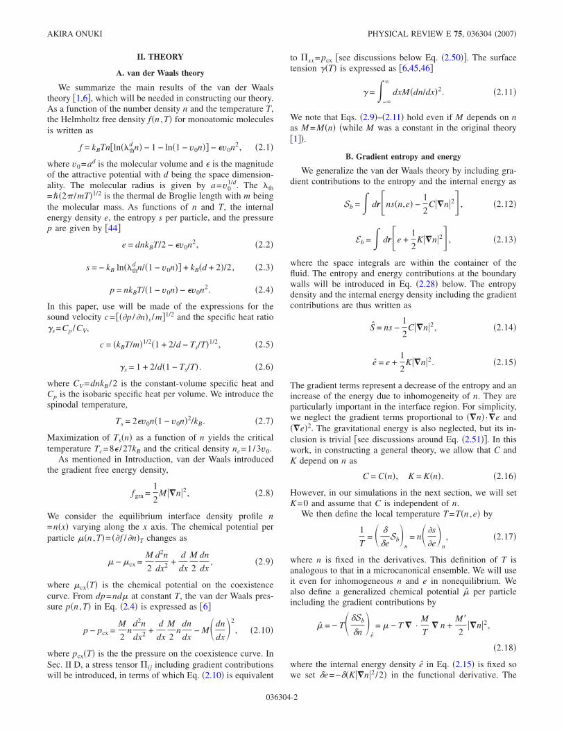
FIG. 1. Density profiles in phase separation after lowering of theboundary temperature from 1.1Tc to 0.91Tc at t=0. Here the liquidlayer �in black� at the boundary acts as a piston adiabatically ex-panding the interior.

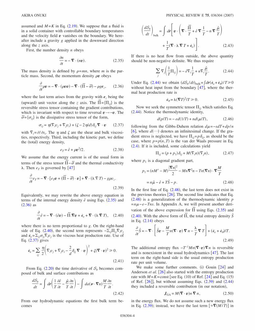
FIG. 2. Adiabatic time evolution of the temperature T and thedensity n at the cell center �lower solid lines� in the early stage afterlowering of the boundary temperature from 1.1Tc to 0.91Tc. Alsoshown is the inverse isothermal compressibility 1 /KT multiplied byKc=nckBTc �dotted line�. The entropy s per particle �upper line�remains nearly unchanged, indicating that the process is adiabatic.The sc is the critical value. All the quantities are those at the cellcenter still without domains in this early stage.

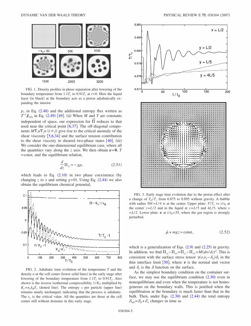
FIG. 3. Early stage time evolution due to the piston effect aftera change of Tb /Tc from 0.875 to 0.895 without gravity. A bubblewith radius 50�=L /4 is at the center. Upper plate: T /Tc vs t / t0 atthe center y=L /2 and in the liquid at y=L /5 and 4L /5, where x=L /2. Lower plate: v at t / t0=55, where the gas region is stronglyperturbed.


036304-5

dStot

dt=� dr

�� + �v

T+� da

� · � � T + es

T, �2.53�

where es=�es /�t= ��es /�n��n /�t. On the right-hand side, thefirst term is the entropy production rate in the bulk, while thesecond term is due to the heat flux from outside and surfaceenergy change. Note that the relation �2.53� holds even whenthe temperature is inhomogeneous on the boundary walls.

III. NUMERICAL RESULTS

A. Method

We integrated the hydrodynamic equations �2.35�, �2.36�,and �2.39� in two dimensions on a 202�202 lattice. Weassume that C in Eq. �2.12� is a constant independent of nand K in Eq. �2.13� vanishes. The mesh size of our simula-tion cell is chosen to be

� = �C/2kBv0�1/2. �3.1�

The interface thickness in two phase coexistence is of order� far from the critical point and is given by �8Tc /27�Tc

−T��1/2� close to the critical point. The system length is L=202�, so our system is very small. In the following figures,the x axis is in the horizontal direction, while the y axis is inthe vertical direction, with 0�x�L and 0�y�L. The ve-locity field v is assumed to vanish on the walls; then, theaverage number density �n�=�drn /V is a conserved quantity.Hereafter �¯� denotes taking the space average. As theboundary condition for the density, we assume Eq. �2.34� inthe form

2�2�� · �n = n − 5nc/2, �3.2�

on all the walls. This yields as=�kBT /2�2 and bs=2v0as inEq. �2.33�. Then the boundary walls are wetted by liquid inequilibrium. The boundary condition for the temperature isas follows. In Figs. 1 and 2, we assume a common boundarytemperature on all the walls. In Figs. 3–15, the bottomboundary temperature Tb at y=0 and the top boundary tem-

perature Tt at y=L will be taken to be different, while theside walls are thermally insulating or � ·�T=0 at x=0 and L.We use the words “top” and “bottom” even in the absence ofgravity.

The transport coefficients strongly depend on the density�30,51�. That is, the shear viscosity and the thermal conduc-tivity of liquid are usually much larger than those in gasexcept in the vicinity of the critical point. For simplicity, weassume them to be proportional to n as

� = � = �0mn , �3.3�

� = kB�0n . �3.4�

Here the kinematic viscosity �0=� /� is assumed to be inde-pendent of n. For example, the liquid and gas densities aren�=1.70nc and ng=0.27nc in two phase coexistence at T

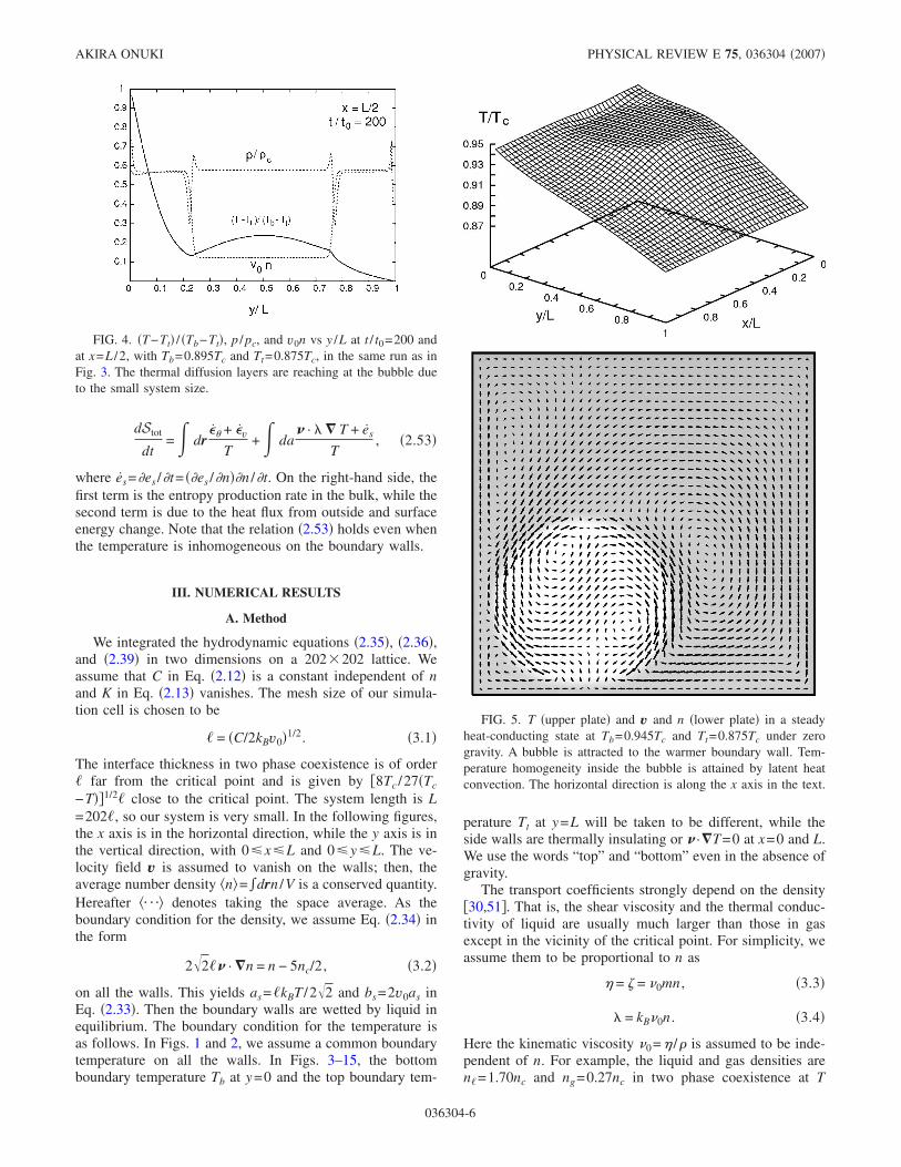
FIG. 4. �T−Tt� / �Tb−Tt�, p / pc, and v0n vs y /L at t / t0=200 andat x=L /2, with Tb=0.895Tc and Tt=0.875Tc, in the same run as inFig. 3. The thermal diffusion layers are reaching at the bubble dueto the small system size.

FIG. 5. T �upper plate� and v and n �lower plate� in a steadyheat-conducting state at Tb=0.945Tc and Tt=0.875Tc under zerogravity. A bubble is attracted to the warmer boundary wall. Tem-perature homogeneity inside the bubble is attained by latent heatconvection. The horizontal direction is along the x axis in the text.


036304-6

=0.875Tc in the van der Waals model. Thus, under Eqs. �3.3�and �3.4� in the van der Waals model, the transport coeffi-cients in liquid are larger than those in gas by 1.70/0 /27=6.3 at T=0.875Tc. Not close to the critical point, the ther-mal diffusion constant DT=� /Cp is of order �0, where theisobaric specific heat Cp per unit volume is of order kBn.Therefore, the Prandtl number Pr=� /�DT is of order unityboth in gas and liquid far from the critical point under Eqs.�3.3� and �3.4�.

We will measure time in units of t0 defined by

t0 = �2/�0, �3.5�

which is the viscous relaxation time �� thermal diffusiontime for Pr�1� on the scale of �. See Appendix B, where wewill rewrite our hydrodynamic equations in dimensionless

forms. We then obtain a dimensionless number,

= �02m/��2 = m�2/�t0

2. �3.6�

For He3 near the gas-liquid critical point with Tc=3.32 K,we have 1/2�=�0�m /��1/2=2.03�10−8 cm by setting �=27kBTc /8. In this paper we set =0.01 �see the sentencesbelow Eq. �3.9� below for its reason�. The normalized gravityacceleration reads

g* = mg�/� , �3.7�

which is the gravity energy of a molecule over the distance ldivided by the van der Waals energy �. For He3 we haveg*=3.2�10−6� with � in units of cm under the earth gravityg=0.98�103 cm3/s. Thus g* is extremely small unless � islarge, which means that the gravity can be relevant only onmacroscopic scales. In Figs. 9–15 below, however, we willset g*=10−4 to induce appreciable gravity effects even forour small system size.

In terms of we express the sound velocity c as

c = As −1/2�/t0, �3.8�

where As is of order unity since Eq. �2.5� gives

As = �kB�2T − Ts�/��1/2/�1 − v0n� �3.9�

in two dimensions. Therefore, the acoustic oscillation be-comes apparent for small , but we require that the acoustictraversal time L /c should be much longer than the micro-scopic time t0 even for our small system length L to obtain 1/2L /��1. A plane wave sound with small wave number q,evolves in time as exp��qt� with �q= ± icq−�sq

2 /2 in a ho-mogeneous one-phase state. The sound damping coefficient�s is written as �s= ��+ �2−2/d�� /�+DT��s−1� �6�. If weuse Eqs. �3.3� and �3.4�, we find

t0�q = ± iAs −1/2Q − �2 − 1/�s�Q2, �3.10�

where Q=�q is the scaled wave number. Therefore, in oursimulation, the damping takes place on the time scale t0 /Q2

and the acoustic oscillation can be seen for Q� −1/2. Fur-thermore, the capillary wave frequency �q��q3 /mn��1/2�in two phase states behaves as �46�

t0�q � �1 − T/Tc�3/4 −1/2Q3/2. �3.11�

The right-hand side gives the deformation rate of a dropletdue to the surface tension if Q=q��2�� /R with R being thedroplet radius.

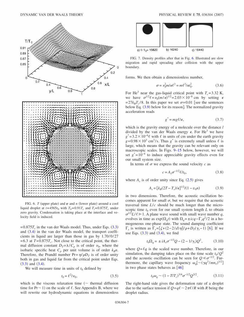
FIG. 7. Density profiles after that in Fig. 6. Illustrated are slowmigration and rapid spreading after collision with the upperboundary.

FIG. 6. T �upper plate� and v and n �lower plate� around a coolliquid droplet at t=4565t0 with Tb=0.91Tc and Tt=0.875Tc underzero gravity. Condensation is taking place at the interface and ve-locity field is induced.


036304-7

B. Phase separation by adiabatic expansion at g=0

First, we investigate phase separation induced by the pis-ton effect �52� taking place upon lowering of the boundarytemperature. In such situations, due to contraction of thermalboundary layers, the interior can be expanded into metastableor unstable states adiabatically �6�. The piston effect is inten-sified near the critical point owing to the divergence of iso-baric thermal expansion. With this method in near-criticalone-component fluids, nucleation experiments were per-formed by Moldover et al. �53�, while spinodal decomposi-tion experiments were realized in space by Beysens et al.�54�. Recently Miura et al. �55� measured adiabatic densitychanges of order 10−7nc in the interior caused by soundpulses in supercritical states. In this paper, however, wepresent an example of adiabatic spinodal decomposition farbelow the critical point caused by the growth of a wettinglayer.

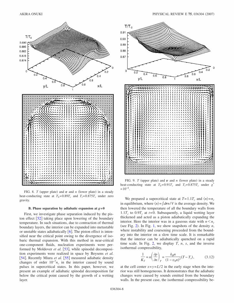
We prepared a supercritical state at T=1.1Tc and �n�=nc

in equilibrium, where �n�=�drn /V is the average density. Wethen lowered the temperature of all the boundary walls from1.1Tc to 0.9Tc at t=0. Subsequently, a liquid wetting layerthickened and acted as a piston adiabatically expanding theinterior. Here the interior was in a gaseous state with n�nc�see Fig. 2�. In Fig. 1, we show snapshots of the density n,where instability and coarsening proceeded from the bound-ary into the interior on a slow time scale. It is remarkablethat the interior can be adiabatically quenched on a rapidtime scale. In Fig. 2, we display T, n, s, and the inverseisothermal compressibility,

1

KT= n� �p

�n�

T=

kBn

�1 − v0n�2 �T − Ts� , �3.12�

at the cell center x=y=L /2 in the early stage when the inte-rior was still homogeneous. It demonstrates that the adiabaticchanges were caused by sounds emitted from the boundarywalls. In the present case, the isothermal compressibility be-

FIG. 8. T �upper plate� and v and n �lower plate� in a steadyheat-conducting state at Tb=0.89Tc and Tt=0.875Tc under zerogravity.

FIG. 9. T �upper plate� and v and n �lower plate� in a steadyheat-conducting state at Tb=0.91Tc and Tt=0.875Tc under g*

=10−4.


036304-8

came negative or brought below the spinodal T�Ts�n� in theearly stage. The acoustic time scale L /c is of order 1/2t0L /��10t0 from Eqs. �3.8� and �3.9�, which agrees withthe oscillation period in Fig. 2.

We make some comments. �i� Though the interior wastransiently close to the critical point in the adiabatic quench-ing in Fig. 2, we neglected the critical fluctuations and thecritical anomaly of the transport coefficients. �ii� Though notshown here, temperature variations are significant among do-mains in the presence of latent heat, while previous simula-tions of spinodal decomposition have been performed in theisothermal condition �6,27,39�. �iii� In our case, a wettinglayer acts as a piston because of its thickening in deepquenching. In near-critical fluids a thermal diffusion layercan well play the role of a piston in supercritical states. If thebulk region is in a liquid state below Tc, a cooled thermaldiffusion layer can even cause phase separation in the inte-rior �54�. By cooling the boundary wall at fixed volume,Moldover et al. �53� could realize homogeneous nucleationin the bulk at liquid densities but could not do so at gasdensities, where the latter result was ascribed to the preexis-tence of a liquid wetting layer. The growth process of a liq-uid wetting layer upon cooling itself has not yet been exam-ined in the literature.

C. Piston effect with a bubble in liquid at g=0

Let us consider the piston effect in the presence of abubble in liquid. When Tb is changed by Tb, sound wavesemitted from the boundary cause a pressure change p. Aftermany traversals of the sounds in the cell, p soon reaches ofthe following order �52�:

p � As�−1Tb, �3.13�

where As� is the liquid value of the adiabatic coefficient As= ��T /�p�s. From Eqs. �2.3� and �2.4� the van der Waalstheory gives

As = � �T

�p�

s=

1/n − v0

kB��1 + d/2� − dTs/2T�. �3.14�

If Tb�0.1Tc and T /Tc�0.9, we find p�0.1pc, which is10 times larger than the Laplace pressure difference � /R forR�50� �46�. Here, due to the different values of As in thetwo phases, there arises a considerable temperature differ-ence in the two regions,

��T�g� = �Asg − As��p , �3.15�

in the early stage. For example, AskB /v0 is equal to 7.1 forgas and 0.65 for liquid at T=0.875Tc from Eq. �3.14� in twodimensions. On the other hand, near the critical point, Asg−As� tends to zero as 2�s

−1/2��T /�p�V, where �s is the specificheat ratio �6�. Thus, the bubble temperature becomes higher�lower� than in the surrounding liquid for positive �negative�Tb. For the case of a liquid droplet, as will be shown in Fig.6, the droplet temperature becomes lower �higher� than in thesurrounding gas for positive �negative� Tb.

In Figs. 3 and 4, we prepared a bubble with radius R=50�=L /4 in equilibrium at T=0.875Tc under zero gravity.We then changed Tb to 0.895Tc for t�0 with Tt held un-changed. In the upper plate of Fig. 3, the bubble center ismore heated than in the liquid at y=L /5 and 4L /5 in theearly stage in accord with Eq. �3.15�. We notice that theoscillation persists within the bubble for a longer time thanin the liquid region. The lower panel of Fig. 3 shows thevelocity field induced by the sounds at t=55t0, which islarger within the bubble than outside it. The typical velocitywithin the bubble is a few times larger than ��v2�=0.011� / t0 at this time. It indicates the presence of appre-ciable mass flux through the interface and suggests existenceof collective modes with evaporation and condensation local-ized near a bubble. In Fig. 4, we show �T−Tt� / �Tb−Tt�,p / pc, and v0n vs y /L at t=200t0 and x=L /2. Here, the os-cillation is mostly damped, while the temperature inside thebubble is not yet flat. We also notice that the thermal diffu-sion layer is thickened up to the bubble, since the distancebetween the bottom and the bubble is narrow. It would takean extremely long time for macroscopic separation. Whilethe temperature is continuous, the pressure is slightly higherinside the bubble than outside it by � /R�0.01pc and exhib-its a singularity in the interface region. The latter behaviorcan be seen in the equilibrium relation �2.10�, from whichthe integral of p in the interface region in the normal direc-tion is equal to −3� /2 for constant M.

D. Two-phase states in heat flow at g=0

In our previous work �15,16�, we examined the tempera-ture and velocity field around a droplet in heat flow. Wesummarize the main results there. Under zero gravity, weshowed numerically and analytically that a gas �liquid� drop-let slowly moves to the warmer �cooler� boundary and thatthe temperature becomes nearly homogeneous within thedroplet. Let a gas droplet �bubble� with radius R be placed ina heat flux Q=−��T� , where �� is the liquid thermal conduc-tivity and T� is the temperature gradient far from the droplet.A convective velocity of order

vc = Q/ngT�s = − ��T� /ngT�s �3.16�

is induced within the droplet, where �s=sg−s� is the entropydifference per particle between the two phases. The velocityvc characterizes latent heat flow and is independent of thebubble radius. The Reynolds number Re=vc�gR /�g is lessthan unity for R��gT�s /mQ, where �g=mng and �g are themass density and the shear viscosity, respectively, in the gasphase.

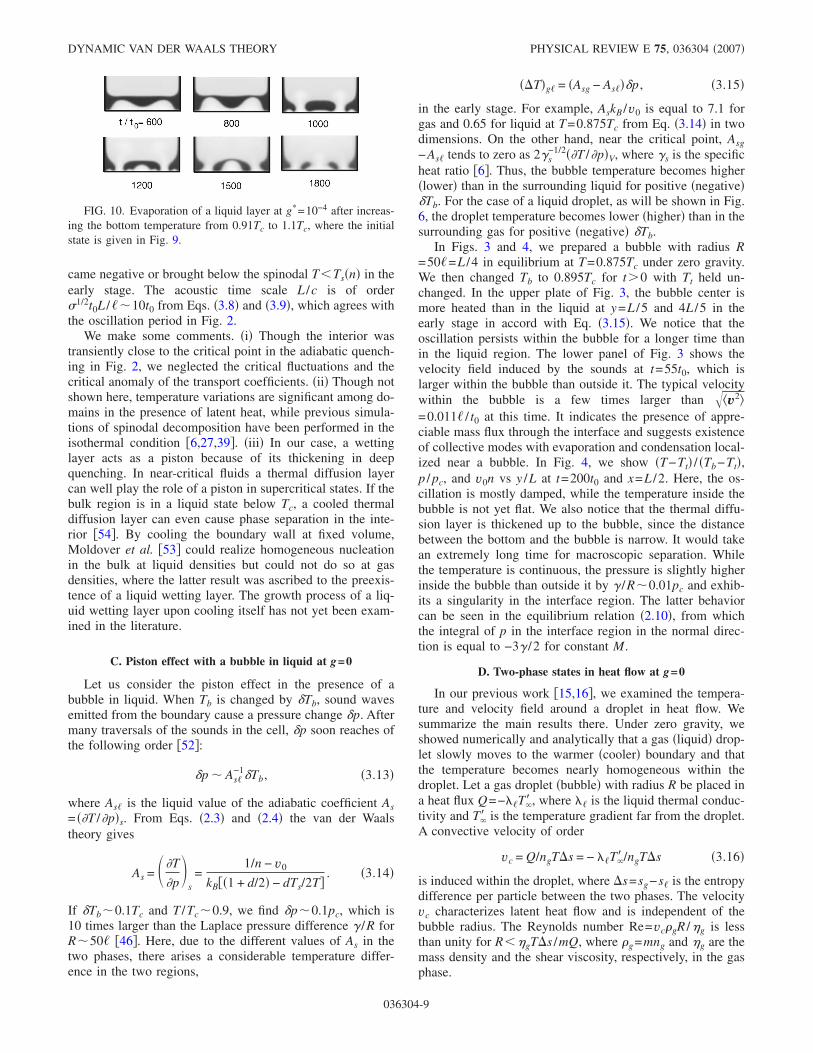
FIG. 10. Evaporation of a liquid layer at g*=10−4 after increas-ing the bottom temperature from 0.91Tc to 1.1Tc, where the initialstate is given in Fig. 9.


036304-9

In our simulation Re is smaller than unity. In Figs. 5–8,we examine heat-conducting two-phase states at zero gravity,where the top temperature at y=L is fixed at Tt=0.875Tc andthe bottom temperature Tb at y=0 is changed to a highervalue. In Fig. 5, we initially prepared a bubble with radiusR=50� in equilibrium at T=0.875Tc at the cell center. Wethen raised Tb to a high value, 0.945Tc, for t�0 to inducedroplet motion toward the bottom. The time scale of migra-tion was about 104t0. Eventually, the droplet partially wettedthe bottom plate with an apparent contact angle. However,Fig. 5 shows the presence of a thin gas layer sandwichedbetween them. The typical velocity in Fig. 5 is given by��v2�=0.029� / t0, which is of order vc in Eq. �3.16�. We cansee that T is flat inside the bubble and continuous across theinterface. The generalized chemical potential � in Eq. �2.18�exhibits the same behavior �not shown here�. The pressure isnearly constant outside the bubble at p�0.76pc, while it isslightly higher inside by � /R�0.01pc �46�. With further in-creasing Tb, the apparent contact angle decreases and thebottom wall is eventually wetted completely by gas. Seesuch an example of complete wetting at Tb=0.97Tc in Ref.�15�. As a related experiment, Garrabos et al. observed thatgas spreads on a heated wall initially wetted by liquid andexhibits an apparent contact angle �10�.

Next, we initially prepared a liquid droplet i gas with R=50� at the cell center at T=0.875Tc and then raised Tb to0.91Tc for t�0. In Fig. 6, we show T, v, and n around aliquid droplet suspended in gas at t=4565t0. Here the veloc-ity field is nearly steady and, as in the lower panel of Fig. 3,it is much smaller in the liquid than that in the gas due to theviscosity difference from Eq. �3.3�. The average velocity am-plitude is given by ��v2�=0.015� / t0 at this time. The tem-perature inside the droplet is nearly homogeneous and islowest in the cell, while the pressure inside it is again onlyslightly higher than outside it by � /R�0.01pc. Hence, con-densation is taking place at the interface and the temperatureinside it is slowly increasing in time as 0.849Tc, 0.851Tc, and0.855Tc at t / t0=4565, 7770, and 15820, respectively, on thetime scale of thermal diffusion ��R2 /D� t0R2 /�2�. Note thatthe initial temperature lowering inside the liquid droplet canbe explained by the adiabatic relation �3.15� �see the argu-ments around it�. In Fig. 7, we show three snapshots of thedensity at later times in the same run as in Fig. 6. The dropletmigration to the cooler wall is very slow, but after its en-counter with it the liquid spreads over it rather rapidly underthe wetting condition �3.2�. In this process the warmerboundary remains dried.

E. Heat conduction in steady two-phase states

Even when the liquid volume fraction is small, efficientheat transport is realized in the presence of evaporation onthe warmer boundary and/or condensation on the coolerboundary. This is the mechanism of heat pipes widely usedin refrigerators and air conditioners. In such processes, thewarmer boundary drys out if evaporation proceeds withoutsupply of liquid. Here we demonstrate that steady heat trans-port with evaporation and condensation can be achieved in aclosed cell in the presence of a liquid wetting layer and/or agravity.

In our situation, we define the effective thermal conduc-tivity through the cell by

�eff = �0

L

dxQb�x�/�Tb − Tt� . �3.17�

As the heat flux, we choose its value at the bottom y=0,

Qb�x� = − ��T/�y�y=0, �3.18�

where v vanishes. It is the heat flux from the bottom bound-ary wall to the fluid. In convection, a normalized effectivethermal conductivity, called the Nusselt number, has beenused to represent the efficiency of heat transport. We define itby

Nu = �eff/��. �3.19�

We take �� as the thermal conductivity at n=1.7nc, which isthe liquid density in two-phase coexistence at T=0.875Tc�see the sentences below Eq. �3.4��. In one-phase states with-out convection, we have Nu=n /1.7nc under Eq. �3.4�. There-fore, Nu is small for gas without convection.

In Fig. 8, we show T, v, and n in a steady heat conductingstate with Tb=0.89Tc and Tt=0.875Tc at zero gravity. A char-acteristic feature in this case is that a liquid layer covers allthe boundary walls. The average density �n�=0.22v0

−1 is rela-tively small. The typical velocity is given by ��v2�=0.0080� / t0. Remarkably, the temperature profile is nearlyflat in the majority gas region, due to latent heat convectionthrough the cell. As a result, Nu=5.0 is realized, despite thefact that the liquid region is only near the boundary walls.

Under gravity, the warmer boundary does not dry outeven for large heat flux. In Fig. 9, we realized a steady statewith �n�=0.206v0

−1 and Tb=0.91Tc under gravity at g*

=10−4, where ��v2�=0.0119� / t0 and Nu=2.0. Again a liquidlayer covers all the boundary walls, while the bottom part isthicker due to the gravity. These features are very differentfrom those in the right panel of Fig. 7 without gravity. In Fig.9, the temperature gradient is large everywhere on the sidewalls and widely in the region y /��0.25 near the bottom,while the liquid-gas interface is at y /��0.1 apart from theside walls. Due to these features we obtain the smaller valueof Nu than for the case in Fig. 8. In Fig. 10, we raised Tb /Tcfrom 0.91 to 1.1 starting with the steady state in Fig. 9. Werecognize that this is the case of strong heating, wherebubbles emerge from the bottom to break the liquid intosmaller pieces. As the gas flow from the bottom is warmer,condensation occurs on the side and top boundary walls,leading to growth of the liquid wetting layer there.

F. Boiling in gravity

Boiling phenomena are very complex and still remain vir-tually unexplored in physics �6,12–14�. Usually, the typicalbubble size is macroscopic and the associated Reynoldsnumber is large. In the present case, we realized boiling un-der gravity at g*=10−4 even for our small system size, wherebubbles from the heated bottom wall were small but couldrise upward with small Reynolds numbers.

In Figs. 11 and 12, we set �n�=0.34v0−1 and held Tt at

0.775Tc. Starting with an equilibrium two-phase state at t


036304-10

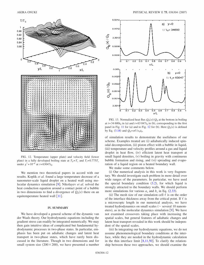
=0, we reached a steady nonboiling state at Tb=0.915Tc,where ��v2�=0.023� / t0 and Nu=3.2 owing to latent heatconvection in the gas region. See the left snapshot at t=104t0 in the upper panels of Fig. 11. We then raised Tb to0.945Tc to produce a weakly boiling state, where a singlebubble periodically appeared with a period about 103t0. Att=27 700t0 a bubble is at the center of the liquid region,while at t=28 010t0 it is being absorbed into the gas region.Here ��v2�=0.033� / t0 and Nu=4.5 at t=27 700t0. Finally, att= tb=34 245t0, we again raised Tb to 1.0Tc. The middle pan-els of Fig. 11 display transition from weak to strong boiling.The bottom plates of Fig. 11 are those in fully developedboiling, which was reached for t− tb�5000t0. In Fig. 12, weshow T, n, and v in fully developed boiling at t=63047t0,where ��v2�=0.055� / t0 and Nu=9.2. We can see steep tem-perature gradients near the boundary walls and large velocitydeviations around the rising bubbles. In Fig. 13, we showthat the heat flux Qb�x� on the bottom in Eq. �3.18� is largewhere rising bubbles are being produced. The upper panel att=34 600t0 is at the inception of strong boiling, exhibiting asharp maximum where a bubble is being detached. The lowerpanel of Fig. 13 at t=63 047t0 is taken in the fully developedboiling state, exhibiting multiple peaks.

In our boiling simulation, the bubble sizes are of orderR�20� and the Reynolds number Re=��v2�R /�0 on thedroplet scale is of order 0.1 in the lower panels in Fig. 11 and

in Fig. 12. Thanks to the high efficiency of latent heat trans-port, the temperature gradient is mostly localized near theboundary walls. Generally in gravity, there should remain asmall temperature gradient in the bulk region in boiling andin stirring. It is given by the so-called adiabatic temperaturegradient �6,14�,

�dT

dz�

bulk= − �g� �T

�p�

s, �3.20�

which is the minimum for the onset of convection for com-pressible fluids �47� and is equal to −0.27 mK/cm for CO2near the critical point. In our case, the right-hand side of Eq.�3.20� is of order −g*Tc /� and is consistent with the averagegradient seen in the upper panel of Fig. 12. In usualRayleigh-Bénard convection in one-phase fluids, the averagetemperature gradient in the bulk region can be suppressedonly in turbulence by rapid convective motion of thermalplumes, where the Reynolds number exceeds unity even onthe scale of the plumes �56�.

G. Wetting dynamics

Wetting dynamics has been studied mostly for involatiledroplets �7�, but it has not yet been well understood for vola-tile droplets or in the presence of evaporation and condensa-tion �8–10�. The previous approaches in the latter case wereby solving the hydrodynamic equations with phenomeno-logical surface boundary conditions �8� and by performingmolecular dynamics simulations of nanometer-size liquiddroplets �9�. Here we present its preliminary numerical studyin our scheme.

At t=0, we placed a semi-circular liquid droplet with R=40� on the bottom, where the interface was on the curve�x−L /2�2+y2=R2. The initial temperature was 0.875Tc

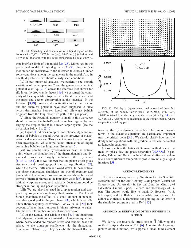
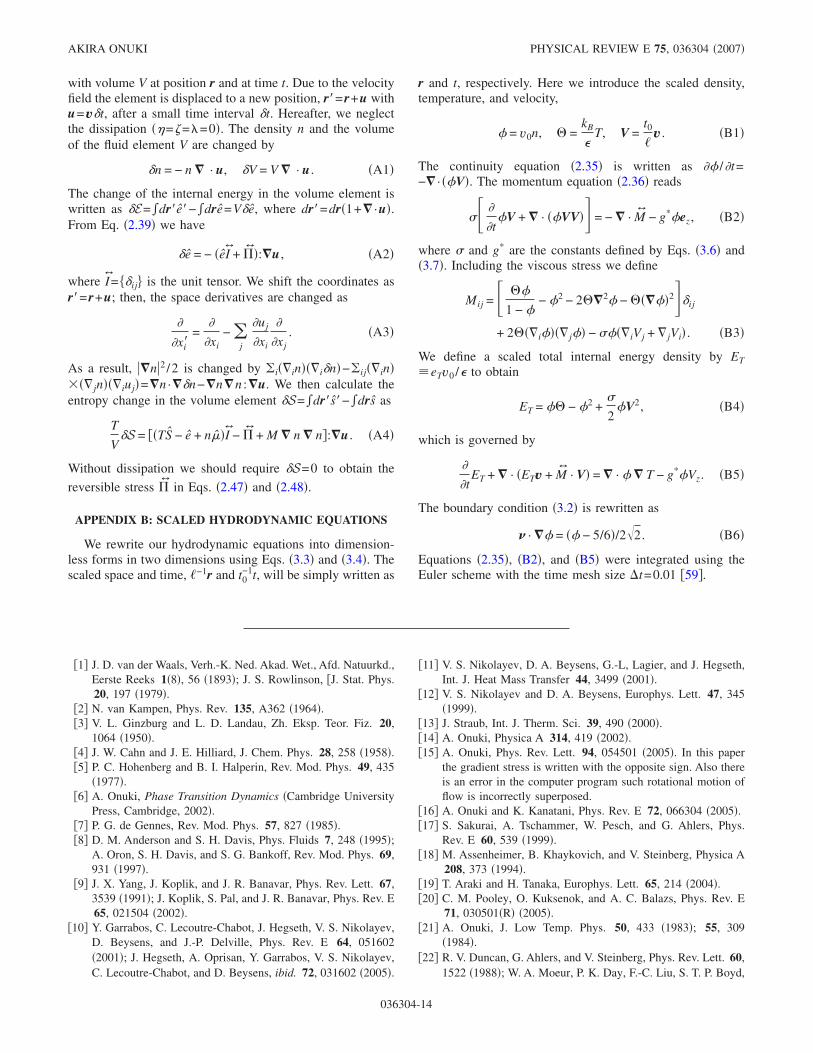
throughout the cell. In the upper panels of Fig. 14, whereboth Tb and Tt were held unchanged, spreading of the liquidregion occurred over the walls on a time scale of 103t0. In themiddle panels of Fig. 14, we set Tb=0.915Tc for t�0 toinduce slow evaporation of the liquid region. We can seeonly a small amount of liquid left on the bottom at t=4000t0 �right�. In the bottom panels of Fig. 14, where Tb=0.975Tc for t�0, a gas droplet appeared within the liquidregion and, as it grew, the liquid region itself was finallydetached from the boundary �right�. In these processes, aconsiderable amount of liquid was evaporating even for thefirst case of Tb=Tt=0.875Tc and the latent heat needed forevaporation was supplied from the equitemperature bound-ary wall. In all these examples, the liquid region was itselfcooled even below the top temperature Tt=0.875Tc by anamount typically of order 0.05Tc. In Fig. 15, we show thevelocity v �upper panel� and the heat flux Qb�x� �lowerpanel� at t=500t0 obtained from the run giving the series �a�in Fig. 14. We can see a circulating flow in the gas and largeheat absorption at the contact points. The peak height ofQb�x� gradually decreased with spreading. These stem fromevaporation at the contact points and condensation on the topof the droplet. The flow pattern here is very different fromthat for involatile droplets �7�.

FIG. 11. Changeovers of boiling with increasing Tb at Tt

=0.775Tc and g*=10−4. Upper plates: nonboiling state at Tb

=0.91Tc �left�, and weakly boiling state with a single bubble at Tb

=0.945Tc �middle and right�. Middle plates: transition from weak tostrong boiling after a change of Tb from 0.945Tc to 1.0Tc at t=34245t0. Lower plates: dynamical steady state with continuousbubble formation and rising.


036304-11

We mention two theoretical papers in accord with ourresults. Koplik et al. found a large temperature decrease of ananometer-scale liquid droplet on a heated wall using mo-lecular dynamics simulation �9�. Nikolayev et al. solved theheat conduction equation around a contact point of a bubblein two dimensions to find a divergence of Qb�x� there on anequitemperature heated wall �11�.

IV. SUMMARY

We have developed a general scheme of the dynamic vander Waals theory. Our hydrodynamic equations including thegradient stress can readily be integrated numerically. We maythen gain intuitive ideas of complicated but fundamental hy-drodynamic processes in two-phase states. In particular, em-phasis has been put on adiabatic changes and latent heattransport in two-phase states, which have rarely been dis-cussed in the literature. Though in two dimensions and forsmall system size �200�200�, we have presented a number

of simulation results to demonstrate the usefulness of ourscheme. Examples treated are �i� adiabatically induced spin-odal decomposition, �ii� piston effect with a bubble in liquid,�iii� temperature and velocity profiles around a gas and liquiddroplet in heat flow, �iv� efficient latent heat transport atsmall liquid densities, �v� boiling in gravity with continuousbubble formation and rising, and �vi� spreading and evapo-ration of a liquid region on a heated boundary wall.

We make some comments below.�i� Our numerical analysis in this work is very fragmen-

tary. We should investigate each problem in more detail overwide ranges of the parameters. In particular, we have usedthe special boundary condition �3.2�, for which liquid isstrongly attracted to the boundary walls. We should performmore simulations for various as and bs in Eq. �2.33�.

�ii� The mesh size of our simulation cell � is on the orderof the interface thickness away from the critical point. If � isa microscopic length in our numerical analysis, we havetreated hydrodynamics on small scales �� several 10 nanom-eters�, as in the molecular dynamics simulation �9�. We havenot examined crossovers taking place with increasing thespatial scales, but general features of adiabatic changes andlatent heat transport revealed in this work should be indepen-dent of the spatial scales.

�iii� In integrating our hydrodynamic equations, we do notassume phenomenological boundary conditions at the inter-face, while they are needed in the hydrodynamic calculationin the thin interface limit �8,11,50�. To clarify the relation-ship between these two approaches, we should examine the

FIG. 12. Temperature �upper plate� and velocity field �lowerplate� in a fully developed boiling state at Tb=Tc and Tt=0.775Tc

under g*=10−4 at t=63047t0.

FIG. 13. Normalized heat flux Qb�x� /Q0 at the bottom in boilingat t=34 600t0 in �a� and t=63 047t0 in �b�, corresponding to the firstpanel in Fig. 11 for �a� and to Fig. 12 for �b�. Here Qb�x� is definedby Eq. �3.18� and Q0=�� /v0t0.


036304-12

thin interface limit of our model �26–28�. Moreover, in thephase field model of crystal growth �31–33�, the interfacemotion can be insensitive to the interface thickness � undersome conditions among the parameters in the model. Also inour fluid problems, we should clarify such conditions.

�iv� In our numerical analysis, we evidently see smoothvariations of the temperature T and the generalized chemicalpotential � in Eq. �2.18� across the interface �not shown for��. In our hydrodynamic theory �16�, we assumed the conti-nuity of these quantities together with the stress balance andthe mass and energy conservation at the interface. In theliterature �8,29�, however, discontinuities in the temperatureand the chemical potential have been supposed to ariseacross the interface between liquid and dilute gas �whichoriginate from the long mean free path in the gas phase�.

�v� Since the Reynolds number is small in this work, weshould examine the high-Reynolds-number regime by en-larging the droplet size R in a much larger system �see thediscussion below Eq. �3.16��.

�vi� Figure 3 indicates complex nonspherical dynamic re-sponse of bubbles to sound waves in the presence of evapo-ration and condensation. This aspect seems to have not yetbeen investigated, while large sound attenuation of liquidcontaining bubbles has long been discussed �6�.

�vii� We should study hydrodynamics near the criticalpoint, where the singularities of the thermodynamic and dy-namical properties largely influence the dynamics�6,10,12,14,54�. It is well-known that the piston effect givesrise to critical speeding-up of thermal equilibration �52�,while the thermal diffusion is slowed down. In near-criticalone-phase convection, significant are overall pressure andtemperature fluctuations propagating as sounds on birth andarrival of thermal plumes at the boundary walls �56�. In near-critical two-phase states, such adiabatic fluctuations could bestronger in boiling and phase separation.

�viii� We are also interested in droplet motion and two-phase hydrodynamics in binary fluid mixtures. Marek andStraub examined the effect of a small amount of noncon-densable gas doped in the gas phase �43�, which drasticallyalters thermocapillary convection. Pooley et al. �20� tookaccount of latent heat transport in binary mixtures to calcu-late the Nusselt number in two-phase convection.

�ix� In the Landau and Lifshitz book �47�, the linearizedhydrodynamic equations are treated as Langevin equations,where newly added are random stress and random heat fluxrelated to the transport coefficients via the fluctuation-dissipation relations �6�. They describe the thermal fluctua-

tions of the hydrodynamic variables. The random sourceterms in the dynamic equations are particularly importantnear the critical point �5,6�. We should clarify how our hy-drodynamic equations with the gradient stress can be treatedas Langevin equations.

�x� We mention the lattice-Boltzmann method devised totreat two-phase flow and phase separation �20,57,58�. In par-ticular, Palmer and Rector included thermal effects to calcu-late a nonequilibrium temperature profile around a gas-liquidinterface �58�.

ACKNOWLEDGMENTS

This work was supported by Grants in Aid for ScientificResearch and for the 21st Century COE project �Center forDiversity and Universality in Physics� from the Ministry ofEducation, Culture, Sports, Science and Technology of Ja-pan. The author would like to thank D. Beysens, V. S.Nikolayev, and D. Bedeaux for valuable discussions. Theauthor also thanks T. Hamanaka for pointing out an error inthe simulation program used in Ref. �15�.

APPENDIX A: DERIVATION OF THE REVERSIBLESTRESS

We derive the reversible stress tensor �J following themethod in Appendix 6A of Ref. �6�. Adopting the Lagrangepicture of fluid motion, we suppose a small fluid element

FIG. 14. Spreading and evaporation of a liquid region on thebottom with Tb /Tc=0.875 in �a� �top�, 0.915 in �b� �middle�, and0.975 in �c� �bottom�, with the initial temperature being at 0.875Tc.

FIG. 15. Velocity v �upper panel� and normalized heat fluxQb�x� /Q0 at the bottom �lower panel� at t=500t0 with Tb /Tc

=0.875 obtained from the run giving the series �a� in Fig. 14. HereQ0=�� /v0t0. Absorption is maximum at the contact points, whereevaporation is taking place.


036304-13

with volume V at position r and at time t. Due to the velocityfield the element is displaced to a new position, r�=r+u withu=vt, after a small time interval t. Hereafter, we neglectthe dissipation ��=�=�=0�. The density n and the volumeof the fluid element V are changed by

n = − n � · u, V = V � · u . �A1�

The change of the internal energy in the volume element iswritten as E=�dr�e�−�dre=Ve, where dr�=dr�1+� ·u�.From Eq. �2.39� we have

e = − �eIJ+�J �:�u , �A2�

where IJ= ij� is the unit tensor. We shift the coordinates asr�=r+u; then, the space derivatives are changed as

�

�xi�=

�

�xi− �

j

�uj

�xi

�

�xj. �A3�

As a result, ��n�2 /2 is changed by �i��in��in�−�ij��in�� jn��iuj�=�n ·�n−�n�n :�u. We then calculate theentropy change in the volume element S=�dr�s�−�drs as

T

VS = ��TS − e + n��IJ−�J + M � n � n�:�u . �A4�

Without dissipation we should require S=0 to obtain the

reversible stress �J in Eqs. �2.47� and �2.48�.

APPENDIX B: SCALED HYDRODYNAMIC EQUATIONS

We rewrite our hydrodynamic equations into dimension-less forms in two dimensions using Eqs. �3.3� and �3.4�. Thescaled space and time, �−1r and t0

−1t, will be simply written as

r and t, respectively. Here we introduce the scaled density,temperature, and velocity,

= v0n, ! =kB

�T, V =

t0

�v . �B1�

The continuity equation �2.35� is written as � /�t=−� · � V�. The momentum equation �2.36� reads

�

�t V + � · � VV� = − � · MJ − g* ez, �B2�

where and g* are the constants defined by Eqs. �3.6� and�3.7�. Including the viscous stress we define

Mij = !

1 − − 2 − 2!�2 −!�� 2ij

+ 2!��i �� j � − ��iVj + � jVi� . �B3�

We define a scaled total internal energy density by ET�eTv0 /� to obtain

ET = ! − 2 +

2 V2, �B4�

which is governed by

�

�tET + � · �ETv + MJ · V� = � · � T − g* Vz. �B5�

The boundary condition �3.2� is rewritten as

� · � = � − 5/6�/2�2. �B6�

Equations �2.35�, �B2�, and �B5� were integrated using theEuler scheme with the time mesh size �t=0.01 �59�.

�1� J. D. van der Waals, Verh.-K. Ned. Akad. Wet., Afd. Natuurkd.,Eerste Reeks 1�8�, 56 �1893�; J. S. Rowlinson, �J. Stat. Phys.20, 197 �1979�.

�2� N. van Kampen, Phys. Rev. 135, A362 �1964�.�3� V. L. Ginzburg and L. D. Landau, Zh. Eksp. Teor. Fiz. 20,

1064 �1950�.�4� J. W. Cahn and J. E. Hilliard, J. Chem. Phys. 28, 258 �1958�.�5� P. C. Hohenberg and B. I. Halperin, Rev. Mod. Phys. 49, 435

�1977�.�6� A. Onuki, Phase Transition Dynamics �Cambridge University

Press, Cambridge, 2002�.�7� P. G. de Gennes, Rev. Mod. Phys. 57, 827 �1985�.�8� D. M. Anderson and S. H. Davis, Phys. Fluids 7, 248 �1995�;

A. Oron, S. H. Davis, and S. G. Bankoff, Rev. Mod. Phys. 69,931 �1997�.

�9� J. X. Yang, J. Koplik, and J. R. Banavar, Phys. Rev. Lett. 67,3539 �1991�; J. Koplik, S. Pal, and J. R. Banavar, Phys. Rev. E65, 021504 �2002�.

�10� Y. Garrabos, C. Lecoutre-Chabot, J. Hegseth, V. S. Nikolayev,D. Beysens, and J.-P. Delville, Phys. Rev. E 64, 051602�2001�; J. Hegseth, A. Oprisan, Y. Garrabos, V. S. Nikolayev,C. Lecoutre-Chabot, and D. Beysens, ibid. 72, 031602 �2005�.

�11� V. S. Nikolayev, D. A. Beysens, G.-L, Lagier, and J. Hegseth,Int. J. Heat Mass Transfer 44, 3499 �2001�.

�12� V. S. Nikolayev and D. A. Beysens, Europhys. Lett. 47, 345�1999�.

�13� J. Straub, Int. J. Therm. Sci. 39, 490 �2000�.�14� A. Onuki, Physica A 314, 419 �2002�.�15� A. Onuki, Phys. Rev. Lett. 94, 054501 �2005�. In this paper

the gradient stress is written with the opposite sign. Also thereis an error in the computer program such rotational motion offlow is incorrectly superposed.

�16� A. Onuki and K. Kanatani, Phys. Rev. E 72, 066304 �2005�.�17� S. Sakurai, A. Tschammer, W. Pesch, and G. Ahlers, Phys.

Rev. E 60, 539 �1999�.�18� M. Assenheimer, B. Khaykovich, and V. Steinberg, Physica A

208, 373 �1994�.�19� T. Araki and H. Tanaka, Europhys. Lett. 65, 214 �2004�.�20� C. M. Pooley, O. Kuksenok, and A. C. Balazs, Phys. Rev. E

71, 030501�R� �2005�.�21� A. Onuki, J. Low Temp. Phys. 50, 433 �1983�; 55, 309

�1984�.�22� R. V. Duncan, G. Ahlers, and V. Steinberg, Phys. Rev. Lett. 60,

1522 �1988�; W. A. Moeur, P. K. Day, F.-C. Liu, S. T. P. Boyd,


036304-14

M. J. Adriaans and R. V. Duncan, ibid. 78, 2421 �1997�.�23� D. Korteweg, Arch. Neerl. Sci. Exactes Nat., Ser. II 6, 1

�1901�.�24� H. Gouin, in PhysicoChemical Hydrodynamics: Interfacial

Phenomena , edited byM. G. Veralde, NATO Advanced Stud-ies Institute, Series B: Physics �Plenum, New York, 1988�, Vol.174, p. 667; P. Casal and H. Gouin, C. R. Acad. Sci., Ser. II:Mec., Phys., Chim., Sci. Terre Univers 306�2�, 99 �1988�.

�25� D. D. Joseph, Eur. J. Mech. B/Fluids 9, 565 �1990�; D. D.Joseph, A. Huang, and H. Hu, Physica D 97, 104 �1996�.

�26� D. M. Anderson, G. B. McFadden, and A. A. Wheeler, Annu.Rev. Fluid Mech. 30, 139 �1998�.

�27� D. Jasnow and J. Viñals, Phys. Fluids 8, 660 �1996�; R. Chellaand J. Viñals, Phys. Rev. E 53, 3832 �1996�.

�28� D. Jamet, O. Lebaigue, N. Coutris, and J. M. Delhaye, J. Com-put. Phys. 169, 624 �2001�.

�29� D. Bedeaux, E. Johannessen, and A. Rosjorde, Physica A 330,329 �2003�; E. Johannessen and D. Bedeaux, ibid. 330, 354�2003�; 336, 252 �2004�.

�30� A. Asai, K. Shinjo, and S. Miyashita, J. Phys. Soc. Jpn. 75,024001 �2006�.

�31� R. Kobayashi, Physica D 63, 410 �1993�.�32� G. Caginalp, Phys. Rev. A 39, 5887 �1989�; A. Karma and W.

J. Rappel, Phys. Rev. E 57, 4323 �1998�.�33� D. M. Anderson, G. B. McFadden, and A. A. Wheeler, Physica

D 135, 175 �2000�.�34� M. Fixman, J. Chem. Phys. 47, 2808 �1967�.�35� L. P. Kadanoff and J. Swift, Phys. Rev. 166, 89 �1968�.�36� K. Kawasaki, Prog. Theor. Phys. 41, 1190 �1969�.�37� B. U. Felderhof, Physica �Amsterdam� 48, 541 �1970�.�38� R. Perl and R. A. Ferrell, Phys. Rev. A 6, 2358 �1972�.�39� T. Ohta and K. Kawasaki, Prog. Theor. Phys. 59, 362 �1978�.�40� A. Onuki, Phys. Rev. A 35, 5149 �1987�.�41� Pep Espaöl, J. Chem. Phys. 115, 5392 �2001�.�42� L. P. Pitaevskii, Zh. Eksp. Teor. Fiz. 40, 646 �1961� �Sov.

Phys. JETP 13, 451 �1961��.�43� R. Marek and J. Straub, Int. J. Heat Mass Transfer 44, 619

�2002�.�44� For diatomic molecules such as O2 the kinetic energy contri-

bution to e should be 5nkBT /2 due to the two rotational de-grees of freedom. For polyatomic molecules such as CO2 itshould be 3nkBT.

�45� You-Xiang Zuo and E. H. Stenby, Fluid Phase Equilib. 132,139 �1997�; S. B. Kiselev and J. F. Ely, J. Chem. Phys. 119,8645 �2003�.

�46� H. Kitamura and A. Onuki, J. Chem. Phys. 123, 124513�2005�. The approximation �=A�a1−d�1−T /Tc�3/2 with A=0.24�M /ad+2kBT�1/2 holds within a few percents in the range0.6�T /Tc�1 for the van der Waals model. Here M is as-sumed to be independent of n. For example, �=0.02�� /v0 atT /Tc=0.85 in terms of � in Eq. �3.1�.

�47� L. D. Landau and E. M. Lifshitz, Fluid Mechanics �Pergamon,New York, 1959�.

�48� J. W. Cahn, J. Chem. Phys. 66, 3667 �1977�.�49� From the argument of the entropy production rate only, our

heat flux Je in Eq. �2.39� and our diagonal pressure p1 in Eq.�2.48� may be generalized to Je�=Je+"JGA and p1�= p1

+"n�n ·��M /T�, where " is arbitrary. The expressions inRefs. �24,26� follow for "=1. However, the arguments in Ap-pendix A lead to "=0.

�50� D. Bedeaux, Adv. Chem. Phys. 64, 47 �1986�. Here a system-atic derivation is given for the surface stress tensor and thesurface boundary conditions.

�51� R. B. Bird, W. E. Stewart, and E. N. Lightfoot, TransportPhenomena �Wiley, New York, 2002�, p. 272.

�52� A. Onuki, H. Hao, and R. A. Ferrell, Phys. Rev. A 41, 2256�1990�; A. Onuki and R. A. Ferrell, Physica A 164, 245�1990�.

�53� D. Dahl and M. R. Moldover, Phys. Rev. Lett. 27, 1421�1971�; J. S. Huang, W. I. Goldburg, and M. R. Moldover, ibid.34, 639 �1975�.

�54� P. Guenoun, B. Khalil, D. Beysens, Y. Garrabos, F. Kommoun,B. Le Neindre, and B. Zappoli, Phys. Rev. E 47, 1531 �1993�;D. Beysens, Y. Garrabos, V. S. Nikolayev, C. Lecoutre-Chabot,J. P. Delville, and J. Hegseth, Europhys. Lett. 59, 245 �2002�.

�55� Y. Miura, S. Yoshihara, M. Ohnishi, K. Honda, M. Matsumoto,J. Kawai, M. Ishikawa, H. Kobayashi, and A. Onuki, Phys.Rev. E 74, 010101�R� �2006�.

�56� A. Furukawa and A. Onuki, Phys. Rev. E 66, 016302 �2002�.�57� D. H. Rothman and S. Zaleski, Rev. Mod. Phys. 66, 1417

�1994�.�58� B. J. Palmer and D. R. Rector, Phys. Rev. E 61, 5295 �2000�.�59� As a technique increasing the numerical stability, we defined

q��T on the midpoints �i+1/2 , j+1/2�, where �i , j� repre-sent the lattice points. For example, qx at the middle point �i+1/2 , j+1/2� was defined by ��i+1, j+1�+��i , j+1�+��i+1, j�+��i , j��T�i+1, j+1�−T�i , j+1�+T�i+1, j�−T�i , j�� /8.Then �x��xT at the point �i , j� was set equal to �qx�i+1/2 , j+1/2�−qx�i−1/2 , j+1/2�+qx�i+1/2 , j−1/2�−qx�i−1/2 , j−1/2�� /2. The same technique was also used for �m��vk.


036304-15

dynamic van der waals theory - 京都大学理学研...

Documents