dynamic switching-based data forwarding for low-duty-cycle

1

Dynamic Switching-based Data Forwarding forLow-Duty-Cycle Wireless Sensor Networks

Yu Gu Member, IEEE, and Tian He, Member, IEEE

Abstract—In this work, we introduce the concept of Dynamic Switch-based Forwarding (DSF) that optimizes the (i) expected data deliveryratio, (ii) expected communication delay, or (iii) expected energy consumption for low-duty-cycle wireless sensor networks under unreliablecommunication links. DSF is designed for networks with possibly unreliable communication links and predetermined node communicationschedules. To our knowledge, these are the most encouraging results to date in this new research direction. In this paper, DSF is evaluatedwith a theoretical analysis, extensive simulation, and physical testbed consisting of 20 MicaZ motes. Results reveal the remarkable advantageof DSF in extremely low duty-cycle sensor networks in comparison to three well-known solutions (ETX [1], PRR×D [2] and DESS [3]). Wealso demonstrate our solution defaults into ETX in always-awake networks and DESS in perfect-link networks.

Index Terms—Wireless Sensor Networks, Low-Duty-Cycle Networks, Dynamic Data Forwarding.

F

1 INTRODUCTION

Wireless Sensor Networks (WSNs) have been proposedfor use in many long-term applications such as militarysurveillance, assisted living, infrastructure monitoring andscientific exploration, which require a network lifespanthat can range from a few months to several years. Onthe other hand, sensor devices (e.g., MicaZ and Telos) arenormally equipped with limited power sources due to theirsmall form factor and low-cost requirements. To resolvethe conflict between limited energy and application lifetimerequirements, it is necessary to reduce node communicationand sensing duty cycles. With the growing gap betweenapplication requirements and the slow progress in batterycapacity [5], there are an increasing number of extremelylow duty-cycle sensor networks designed and deployed.Together with lossy radio links, these new networks imposenew challenges for data forwarding protocols.

In this work, we focus on low-duty-cycle sensor networkswith unreliable communication links, in which energy man-agement protocols [6], [7], [8] schedule sensing and commu-nication at each individual sensor device to enable a dutycycle of 10% or less. Essentially, during the operation ofsensor applications, sensor nodes activate very briefly andstay in a dormant state for a very long period of time. Dueto the devices’ extremely limited energy budget, maintain-ing an always-awake communication backbone becomesinfeasible. Consequently to forward a packet, a sender mayexperience sleep latency – the time spent waiting for thereceiver to wake up.

In this paper we attempt to design a new data deliverymethod to optimize source-to-sink data delivery ratio, end-to-end (E2E) delay, or energy consumption under unreliableand intermittent connectivity within scheduled networks.

• Yu Gu is with Singapore University of Technology and Design, Singapore.Tian He is with University of Minnesota, Twin Cities, USA.E-mail: [email protected], [email protected]

A conference paper [4] containing some preliminary results of this paper hasappeared in ACM SenSys 2007

The major intellectual contributions of this work are asfollows:

• To the best of our knowledge, this is the first work toinvestigate the combined effect of sleep latency and un-reliable communication links, which dramatically reducesthe effectiveness of the existing solutions. A noveldynamic switch-based forwarding technique over time-dependent networks is proposed to achieve optimal ex-pected delivery ratio (EDR), expected E2E delay (EED),or expected energy consumption (EEC), respectively.This technique is generic enough to allow flexibletradeoffs among these three key metrics.

• We extensively evaluate our solutions with 20 MicaZmotes experiments and 250-node simulation. The re-sults from experiments and simulations show signifi-cantly better source-to-sink communication than sev-eral state-of-the-art solutions.

The rest of the paper is organized as follows: Section 2presents the related work. Section 3 describes the need fora new data forwarding technique in extremely low duty-cycle sensor networks. Section 4 articulates the networkmodel and related assumptions. Section 5 introduces thedetailed design of DSF and discusses related issues. Sec-tion 7 describes our system implementation and providesan evaluation on the TinyOS/Mote platform. Simulationresults are presented in Section 8. Section 9 concludes thepaper.

2 RELATED WORK

The contribution of our work lies in the intersection of twoimportant cutting-edge research topics. We demonstratethat the intriguing interaction between unreliable links andlow-power duty-cycling necessitates a fundamentally newapproach.

Link-Quality-Based Forwarding: Many recent works [9],[10] reveal that wireless communication links, especiallyfor the low-power sensor devices, are extremely unreliableand have a significant impact on data delivery. In response

to the reality of unreliable wireless links, several notableworks have been done. De Couto et al. introduce theexpected transmission count metric (ETX) to find high-throughput paths on multi-hop wireless networks [1]. Wooet al. show that cost-based routing using a minimumexpected transmission metric obtains good performancein wireless sensor networks [11]. Seada et al. study thedistance-hop trade-off for geographic routing in wirelesssensor networks and show that the product of the packetreception rate (PRR) and the distance traversed toward thedestination (D) is an optimal metric (PRR×D) for selectinga next-hop forwarder [12]. Lee et al. present SOFA, an on-demand solicitation-based forwarding protocol and showthat SOFA outperforms the commonly used link estimation-based routing schemes implemented in TinyOS [13]. InETF [14], Sang et al. exploit asymmetric wireless links andobserve significant improvement of convergecast routing insensor networks. In these works, the authors assume theconstant availability of connectivity with no sleep latency,which may not be true in extremely low duty-cycle sensornetworks.

Sleep-Latency-Based Forwarding: In the research directionof low duty-cycle networks, Dousse et al. provide a solidanalysis of bounds of the delay for sending data from anode to a sink in the networks with completely uncoor-dinated node working schedules [15]. Lu et al. introducevarious techniques for minimizing communication latencywhile providing energy-efficient periodic sleep cycles fornodes in wireless sensor networks [3]. Keshavarzian et al.introduce a multi-parent forwarding technique and proposea heuristic algorithm for assigning parents to the nodesin the network [16]. Lai and Paschalidis propose a mini-mal energy routing with latency guarantees in duty-cycledsensor networks [17]. Su et al. propose both on-demandand proactive algorithms for routing packets in intermit-tently connected sensor networks [18]. Several recent worksstudied multicast and flooding in low-duty-cycle sensornetworks [19], [20]. More recently, Gu et al. study thedelay control for low-duty-cycle sensor networks [21]. Wenote, however, that all these approaches in low duty-cyclenetworking assume perfect communication links.

We note that many MAC protocols, such as B-MAC [22],S-MAC [23] and RI-MAC [24], effectively deal with theissues of lossy radio links through FEC/ARQ and reduceduty-cycle through the Low-Power-Listening (LPL) [22].More recently, Suriyachai et al. introduces a novel MACprotocol that incorporates topology control mechanisms toensure timely data delivery and reliability control mecha-nisms to deal with inherently fluctuating wireless links [25].These intelligent layer 2 protocols use implicit networkinformation, such as packet transmissions, in order to op-timize their underlying schedules or energy use. In thispaper, we consider the dual of this problem by usinginformation from layer 2 at the network layer to make betterlink selections.

In addition, there are many other related works ontimely and reliable data forwarding in sensor networks.MMSPEED introduces a multi-path and multi-speed rout-

ing protocol for probabilistic QoS guarantee [26]. Dwarfachieves energy-efficient, robust and dependable forward-ing by unicast-based partial flooding and delay-aware nodeselection [27]. WirelessHART with TSMP [28] is a deployedindustry standard aiming to achieve timely and reliabletransmission while reducing energy consumption. Munir etal. propose a scheduling algorithm that produces latencybounds of the real-time periodic stream sand accounts forboth link bursts and interference [29].

To the best of our knowledge, no prior work has thor-oughly studied the impact of both lossy radio links and sleeplatency at the network layer. In this work, we reveal thatthese two issues are intrinsically correlated and that a newforwarding protocol can benefit from considering both.

3 MOTIVATION

Our work is motivated by the interesting intersection be-tween sleep latency and unreliable communication links inwireless sensor networks.

0

500

1000

1500

2000

2500

3000

0.01 0.1 1

Avg

. E2E

Del

ay (

unit)

Network Duty Cycle (Percentage)

350m * 350m square field

1000 nodes

ETX

Fig. 1. E2E Delay vs. Network Duty Cycle

First, the state-of-the-art link-quality-based forwardingstrategies such as ETX [1] and PRR×D [2] have demon-strated their superiority at improving network throughputand communication delay in traditional ad hoc and sensornetworks. For both ETX and PRR×D, during a certainperiod of time each node usually has one fixed forwardingnode for a destination. However, in extremely low duty-cycle scheduled sensor networks, metrics such as the ex-pected transmission count (ETX) would suffer excessivedelivery delays when waiting for the fixed receiver to wakeup again if the ongoing packet transmission fails. Figure 1shows the E2E delays from a randomly chosen source nodeto the sink node using ETX forwarding metrics under differ-ent network duty cycles in a randomly-generated networktopology. The simulation setup is the same as in Section 8and key simulation parameters are shown on the figure.The simulation was repeated 1000 times and the averagevalue is reported in Figure 1 (in log-scale), which showsthat as network duty cycle decreases, the E2E delay growssignificantly. For example, at the duty cycle of 100%, theE2E delay of ETX is only 37.6 units of time. In contrast,when the duty cycle drops to 1%, the E2E delay increasesto 2955.5 units of time, which is approximately an 80-foldperformance degradation in end-to-end delay!

Second, sleep-latency-based forwarding [30], [3] ignoresthe reality that wireless radio quality is highly unreliableand that thus the optimality of their approaches holds onlywhen the link quality in the network is perfect. Figure 2shows the E2E delay from a randomly chosen source node

2

0

1000

2000

3000

4000

5000

6000

7000

0.1 0.2 0.3 0.4 0.5 0.6 0.7 0.8 0.9 1

Avg

. E2E

Del

ay (

unit)

Avg. Link Quality (Percentage)

350m * 350m square field

1000 nodes

DESS

Fig. 2. E2E Delay vs. Average Link Quality

to the sink node using delivery methods proposed in [3]under different average link quality in a random generatednetwork topology. As shown in the figure, the E2E delayincreases from 380.0 to 6851.4 units of time while theaverage link quality decreases from 100% to 10%, whichis approximate a 20-fold performance degradation, eventhough global scheduling information is available.

The main observation from our initial studies is thatboth the link quality and the duty cycle of sensor nodescan significantly impact end-to-end communication. Al-though link-quality-based forwarding [1], [2] and sleep-latency-based forwarding [30], [3] have demonstrated theireffectiveness in their own contexts, they fail to deal withthe combined effect exhibited in many real-world sensornetwork applications. This limitation motivates us to designa new data forwarding technique, which we discuss in therest of the paper.

4 MODELS AND ASSUMPTIONS

Before presenting DSF in detail, we present the networkmodel and assumptions used in this work. To simplify ourdescription, we introduce DSF’s design in a synchronizedmode with discrete time. Later on, we explain why DSFworks without time slots and only requires local synchro-nization. In other words, DSF works in CSMA networkswhere nodes are duty-cycled by upper-layer protocols suchas sensing coverage [31] and power management [16], [32],[33].

4.1 Network ModelWe assume a network with N sensor nodes. At a given pointof time t a sensor node is in either an active or a dormantstate. When a node is in the active state, it can sense andreceive packets transmitted from neighboring nodes. Whena node is in the dormant state, it turns off all functionmodules except a timer (for the purpose of waking itselfup). In other words, a node can wake up to transmit apacket at any time, but can receive packets only when it isin its active state. Formally, we denote the network statusat time t as G(t) = (V,E(t)), where V is a complete set ofN nodes within the network, and E(t) is a set of directededges at time t. An edge e(i, j) belongs to E(t) if and only if(1) node ni is a neighboring node of nj , and (2) nj is activeand hence able to receive data at time t. Essentially, G(t)represents the potential traffic flow within the network attime t. Obviously the connectivity of G(t) varies with time.In other words, G(t) is a time-dependent network.

We represent the states of each node ni with a workingschedule Γi = (ωi, τ).

• ωi is an infinite binary string, in which 1 denotes theactive state and 0 denotes the dormant state. Clearly,the duty cycle of a node is the percentage of 1’s in thebinary string. Since the working schedules of the sensornodes are normally periodic (for sensing purposes),the infinite binary string ωi can be described using aregular expression.

• The state transitions between active and inactive statesare time-driven. We use τ to denote the time span a bitin the binary string ωi.

We note that the simple 2-tuple (ωi, τ) is generic enoughto represent arbitrary sensor nodes working schedules.Theoretically, when τ → 0 , ωi can precisely characterize anyon/off behavior of node ni. For clarity of presentation, webegin our design with a simplified assumption that it takestime τ to transmit one packet and receive acknowledgmentfrom a receiver. The assumption on the round-trip trans-mission time bound τ holds well when traffic/congestionis low, which is the case in extremely low duty-cycle sensornetworks. In addition, B-MAC [22] has already used link-level implicit acknowledgement to support fixed round-triptransmission time.

4.2 Time-Expanded Network

To visualize the data delivery process in a time-dependentnetwork G(t) = (V,E(t)), we replicate G(t) with regulargraphs G = (V,E) along with the time dimension. We callthis is a time-expanded network. In this section, for a givensensor network topology and node working schedules, wedescribe how we can build a corresponding time-expandednetwork. The resulting time-expanded network can help usbetter understand the data delivery method introduced inthe rest of the paper.

Given a network G(t) = (V,E(t)) with n nodes andnode working schedules Γi = (ωi, τ), where i ∈ V , weuse the following rules to construct its corresponding time-expanded network.

• For any node i ∈ V at time t, we build a distinct nodeNit.

• For each newly built node Nit, if node j is a neigh-boring node of the node i and p is the position of firstactive bit in ωj after time t, we build a directed edgefrom Nit to Njp with a length of (p− t)τ .

• At the destination node d, we connect all its time-expanded nodes to a null node with edge lengths ofzero.

To illustrate the above network mapping rules, we provide awalk-through of time-expanded network construction froma time dependent graph. Figure 4 shows how to constructa time-expanded network from the linear time-dependentnetwork shown in Figure 3. As shown in Figure 3, for node1 at time 1, the only node that is within its communicationrange is node 2, and its first active state after time 1 appearsat time 3, so in Figure 4, we build a directed edge fromnode 1 at time 1 to node 2 at time 3 with an edge length of2τ . Similarly, we construct other edges in Figure 4. Finally,for the destination node 4, we connect all its time-expanded

3

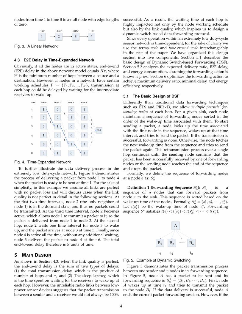
nodes from time 1 to time 6 to a null node with edge lengthsof zero.

1 2 3 4(100)* (010)*(001)* (111)*

Fig. 3. A Linear Network

4.3 E2E Delay in Time-Expanded NetworkObviously, if all the nodes are in active states, end-to-end(E2E) delay in the above network model equals Hτ , whereH is the minimum number of hops between a source and adestination. However, if nodes in a network have certainworking schedules Γ = {Γ1,Γ2, ...,ΓN}, transmission ateach hop could be delayed by waiting for the intermediatereceivers to wake up.

Time

1:

2:

3:

4:

5:

6:

Node 1 Node 2 Node 3 Node 4

1

0

0

1

0

0

0

0

1

0

0

1

0

1

0

0

1

0

1

1

1

1

1

1

Null

2

2

1

2

1

1

000

000

1

1

1

1

1

3

3 1

Fig. 4. Time-Expanded Network

To further illustrate the data delivery process in theextremely low duty-cycle network, Figure 4 demonstratesthe process of delivering a packet from node 1 to node 4when the packet is ready to be sent at time 1. For the sake ofsimplicity, in this example we assume all links are perfectwith no packet loss and will discuss cases when the linkquality is not perfect in detail in the following sections. Atthe first two time intervals, node 2 (the only neighbor ofnode 1) is in the dormant state, and thus no packets couldbe transmitted. At the third time interval, node 2 becomesactive, which allows node 1 to transmit a packet to it, so thepacket is delivered from node 1 to node 2. At the secondhop, node 2 waits one time interval for node 3 to wakeup, and the packet arrives at node 3 at time 5. Finally, sincenode 4 is active all the time, without any additional waiting,node 3 delivers the packet to node 4 at time 6. The totalend-to-end delay therefore is 5 units of time.

5 MAIN DESIGN

As shown in Section 4.3, when the link quality is perfect,the end-to-end delay is the sum of two types of delays:(1) the total transmission delay, which is the product ofnumber of hops and τ , and (2) The sleep latency, whichis the time spent on waiting for the receivers to wake up ateach hop. However, the unreliable radio links between low-power sensor devices suggests that the packet transmissionbetween a sender and a receiver would not always be 100%

successful. As a result, the waiting time at each hop ishighly impacted not only by the node working schedulebut also by the link quality, which inspires us to design adynamic switch-based data forwarding protocol.

Since every operation within an extremely low duty-cyclesensor network is time-dependent, for the sake of clarity weuse the terms node and time-expand node interchangeablyin the rest of the paper. We have organized this designsection into five components. Section 5.1 describes thebasic design of Dynamic Switch-based Forwarding (DSF).Section 5.2 analyzes the expected delivery ratio, E2E delay,and energy consumption, assuming the forwarding action isknown a priori. Section 6 optimizes the forwarding action toachieve maximum delivery ratio, minimal delay, and energyefficiency, respectively.

5.1 The Basic Design of DSFDifferently than traditional data forwarding techniquessuch as ETX and PRR×D, we allow multiple potential for-warding nodes at each hop. For a given sink, each nodemaintains a sequence of forwarding nodes sorted in theorder of the wake-up time associated with them. To startsending a packet, a node looks up the time associatedwith the first node in the sequence, wakes up at that timeinterval, and tries to send the packet. If the transmission issuccessful, forwarding is done. Otherwise, the node fetchesthe next wake-up time from the sequence and tries to sendthe packet again. This retransmission process over a singlehop continues until the sending node confirms that thepacket has been successfully received by one of forwardingnodes or the sending node reaches the end of the sequenceand drops the packet.

Formally, we define the sequence of forwarding nodesat a node e as: Se

n

Definition 1 (Forwarding Sequence Sen): Se

n is asequence of n nodes that can forward packets fromnode e to the sink. This sequence is sorted based on thewake-up time of the nodes. Formally, Se

n = (se1, se2, · · · , sen).

Let t(sei ) be the wake-up time of node sei , Forwardingsequence Se satisfies t(e) < t(se1) < t(se2) < · · · < t(sen).

Bn

A

B1 B2

…...

t1 t2 tnFig. 5. Example of Dynamic Switching

Figure 5 demonstrates the packet transmission processbetween one sender and n nodes in its forwarding sequence.In Figure 5, node A has a packet to be sent and itsforwarding sequence is SA

n = (B1, B2, · · · , Bn). First, nodeA wakes up at time t1 and tries to transmit the packetto the node B1. If the data delivery is successful, node Aends the current packet forwarding session. However, if the

4

transmission fails, the node A wakes up again at time t2 andtries to send the packet to the node B2. This retransmissionprocess continues with node A repeatedly trying to send thepacket to the node in the sequence SA

n . If the transmissionfails at the last node Bn, node A drops the packet.

From the above example, we can see that the majoradvantage of dynamic switching is the use of a forwardingsequence to reduce the time spent on transmitting a packetsuccessfully at each hop rather than waiting for a particularforwarding node to wake up again after failure, as in suchsolutions as ETX, PRR×D and DESS.

5.2 The Modeling of EDR, EED, and EEC

Given a known forwarding sequence Sen at a node e , we can

model the expected delivery ratio, the expected E2E delayand the expected energy consumption for the node. Here,for the sake of clarity, we describe a scenario with a singlesink node, that can be extended easily for scenarios withmultiple sink nodes.

Formally, these three metrics are defined as:

Definition 2 (Expected Delivery Ratio EDRe(Sen)): The

expected delivery ratio at node e for a given forwardingsequence Se

n, denoted by EDRe(Sen), is the expected packet

delivery ratio from node e to the sink node (over multi-hoppath).

Definition 3 (Expected E2E Delay EEDe(Sen)): The

expected E2E Delay at node e for a given forwardingsequence Se

n, denoted by EEDe(Sen), is the expected data

delivery delay for the packets sent by node e and receivedby the sink node (over multi-hop path).

Definition 4 (Expected Energy Consumption EECe(Sen)):

The expected energy consumption at node e for a givenforwarding sequence Se

n, denoted by EECe(Sen), is the

expected energy consumption to deliver a packet fromnode e to the sink node (over multi-hop path). We note thatsince receiving (idle) energy is fixed for a given workingschedule, we include only senders’ transmission energy inEEC.

Our model for computing EDR, EED, and EEC valuesis distributed and can be executed at individual sensornodes independently. At the sink node (b), obviously, itsforwarding sequence is empty, the EDRb(∅) value is 100%(i.e., no packet loss), while EEDb(∅) and EECb(∅) valuesare both zeros (i.e., no delay and no energy consumption).Consequently, we can obtain following initial equations:

EDRb(∅) = 1 , EEDb(∅) = 0 , EECb(∅) = 0 (1)

Let the bi-directional link quality pei denotes the success ra-tio of a round-trip transmission (DATA and ACK) betweennode e and the ith forwarder in Se

n. The link quality peican be influenced by multiple factors such as transmissionpower and the distance between a sender and a receiver.We note that in extremely low duty-cycle sensor networks,traffic congestion is rare and hence has little effect on linkquality.

The overall probability P e(i) that a packet transmissionby node e is successful at the ith forwarder (after i − 1failures) can be represented as:

P e(i) = [i−1∏j=1

(1− pej)]pei (2)

Expected Delivery Ratio (EDR): Obviously, EDR value fornode e is the sum of the product of the probability thatthe transmission is successful at a particular forwarder andits corresponding EDR value for all nodes in Se

n. Assumingnode e has n nodes in its forwarding sequence and lettingEDRi be the EDR value for the ith forwarder (sei ) in Se

n, wehave the following recursive equation for EDRe(S

en).

EDRe(Sen) =

n∑i=1

P e(i)EDRi (3)

Expected E2E Delay (EED): The EED value of node e repre-sents the expected delay for the packets sent by node e thatreach the sink node b. Consequently, the probability that thepacket transmission is successful at a certain forwarder isunder the condition that the packet is delivered by one ofthe forwarders in Se

n. Therefore, the conditional probabilityis P e(i)′ = P e(i)EDRi

EDRe(Sen)

. Letting EEDi be the EED value forthe ith forwarder in node e’s forwarding sequence and dibe the delay for node e to wait node sei in Se

n to wake up,EEDb(S

en) can be represented as:

EEDe(Sen) =

∑ni=1 P

e(i)′(di + EEDi) (4)

Expected Energy Consumption(EEC): Similarly, let EECi

be the EEC value for the ith forwarder in Sen and that

the expected energy consumption for successful packettransmission at node sei is the sum of EECi and i units ofenergy consumption (note that energy wasted in i−1 failedtransmission should be included as well). The probabilitythat the retransmission of a packet reaches the ith forwarderP e(i)′ at node e is conditional on the data delivery ratioEDRe(S

en). Therefore, P e(i)′ = P e(i)EDRi

EDRe(Sen)

, and we canformulate the EECe(S

en) as:

EECe(Sen) =

∑ni=1 P

e(i)′(i+ EECi) (5)

The recursive calculation of EDR, EED and EEC can beimplemented at individual nodes distributively. The mainidea is to radiate known initial conditions (EDRb(∅) = 1,EEDb(∅) = 0,EECb(∅) = 0) from the sink node, so that theprocess of calculating EDR, EED and EEC values propagatesoutward from the sink nodes to the rest of the network.

6 OPTIMIZING THE FORWARDING SEQUENCE

In the previous section, we described the model for calculat-ing EDR, EED, and EEC for a given forwarding sequence.In this section, we will discuss how we can obtain a for-warding sequence that is optimal in terms of the maximumexpected data delivery ratio, minimum expected E2E delay,or minimum expected transmission energy consumption atindividual sensor nodes, respectively.

In practical network settings, especially in low duty-cyclesensor networks, a sender should not endlessly retransmit

5

a packet because it would consume significant energy atthe sending nodes. Therefore, we set the maximum timebound for a sender to retransmit a particular packet as T .Consequently, at node e, with known neighboring nodesand their corresponding working schedule Γ, we can havea full sequence of potential forwarding nodes that wake upbefore T .

Formally, let sei be a next-hop node with wake-up timet(sei ). Node e’s full sequence Se

m under the bound T is:

Sem = (se1, s

e2, · · · , sem) where s ∈ Se

m ⇐⇒ t(e) ≤ t(s) ≤ t(e)+T.

6.1 Optimizing Expected Delivery Ratio (EDR)Because the length of the potential forwarding sequence ofa node is finitely subject to the maximum retransmissiontime interval T , under the reality of unreliable link qualityamong pairs of wireless sensor devices, packets sent bya source node may not all arrive the destination sinknode. Therefore, when reliable transmission has the highestpriority for a sensor network application, the optimizationof the expected data delivery ratio (EDR) is critical.

Intuitively, in order to maximize the expected data de-livery ratio at node e, we should try to send packets aslong as one of the next-hop nodes is awake. The reasoningbehind this is plausible, as since we want to maximizethe expected data delivery ratio, we should take everyopportunity to move the packet out of the sender. However,this intuition does not lead us to an optimal expected datadelivery ratio, and Figure 6 presents a counterexample. InFigure 6, suppose the full forwarding sequence of the nodeS is SS

2 = (A,B). If we choose both node A and B to formS’s forwarding sequence SS

2 , according to the Equation 3,EDRe(S

S2 ) = 10%. In contrast, if we choose only node B to

be included in SS1 , the corresponding EDRe(S

S1 ) = 100%.

Therefore, in order to optimize the expected data deliveryratio at a node e, we shall select a subsequence fromthe full sequence Se

m. By definition, a subsequence canbe obtained by removing some of the elements from theoriginal sequence without disturbing the relative positionsof the remaining elements. As an example, (B,E,D,G) isa subsequence of (A,B,E,C, F,D,H,G).

B

A

S

100%

100%

EDR = 10%

EDR = 100%

Fig. 6. Example for Selecting a Subset of Nodes in PotentialForwarding Sequence

To select an optimal subsequence Seopt from the full

sequence Sem, we adopt a dynamic programming approach.

Clearly, the last node sem in Sem must be included in Se

opt,since sem provides the last chance for node e to retransmitbefore the packet is dropped. Starting from this optimalsubstructure, we can attempt to include nodes (one by

one) from Sem backwardly into Se

opt. If the inclusion of anode from Se

m into Seopt increases EDRe(S

eopt), we then add

this node into Seopt permanently. Otherwise, we discard the

node and try to add the next node. The above forwardingsequence selection process continues until we reach thenode se1 in the full sequence Se

m. The optimality of thisdynamic programming algorithm is based on the fact thatthe optimal EDRe(S

eopt) can be constructed efficiently from

its optimal substructures. The decisions made to include orexclude a later node in the forwarding sequence does not affectthe optimality of decisions made to include or exclude earliernodes and vice versa. For each backward augmentation of theforwarding sequence, we guarantee the maximum data de-livery ratio of the sequence between the newly augmentednode and the last node. This forwarding sequence, then,serves as an optimal substructure for augmenting additionalforwarders until the process reaches the first node in thesequence.

Let Seopt(k) denote the optimal forwarding subsequence in

terms of maximizing EDR metric from the sequence Sek =

(sem−k+1, sem−k+2, . . . , s

em). Obviously, Se

opt(m) is the optimalsubsequence we want to obtain.

We have the following initial optimal substructure:

Seopt(0) = ()

Seopt(1) = (sem)

(6)

Building upon the previous optimal substructure, when weattempt to include the next node sej in Se

m into Seopt(k − 1)

backwardly, there are two possible outcomes:• According to the model of EDRe(S

e), if the appendingof node sej to Se

opt(k−1) increases the expected deliveryratio, we insert node sej in front of the existing sequenceSeopt(k − 1) to obtain Se

opt(k).• If the inclusion of node sej into sequence Se

opt(k − 1)does not increase the data delivery ratio, the optimalforwarding sequence remains unchanged.

Formally, let sej ⊕ S denote inserting node sej to the frontof the sequence S, the corresponding recursive equation forSeopt(k) can be represented as:

Seopt(k) =

Seopt(k − 1) EDRe(S

eopt(k − 1)) >

EDRe(sej ⊕ Se

opt(k − 1))sej ⊕ Se

opt(k − 1) Otherwise(7)

6.1.1 Detailed Algorithm for Optimizing EDRIn the previous section, we discussed recursive equationsfor optimizing forwarding sequence for EDR. In this section,we introduce detailed dynamic programming algorithmthat implements earlier mathematical formulations. Thecomplete algorithm is shown in Algorithm 1. Firstly, accord-ing to the known wake-up time of neighboring nodes, weform a full sequence S−me as the input of our optimizingalgorithm. Then following Equation 6, we construct aninitial optimal substructure (Line 1 to Line 2). From Line4 to Line 14, we perform the task of adding forwardingnode backwardly and decide whether a node should beincluded in the optimal forwarding sequence or not. Line5 to Line 9 constructs a temporary forwarding sequence

6

Algorithm 1 Forwarding sequence optimization for EDR ata time expanded node e

Input: Full sequence Sem, with length m.

Output: The optimal forwarding sequence Se

1: Seopt(0)← ()

2: Seopt(1)← (sem)

3: i← 24: for j from (m− 1) downto 1 do5: if t(sej) ̸= t(seopt(i− 1)) then6: S ← sej ⊕ Se

opt(i− 1).7: else8: S ← sej ⊕ (Se

opt(i− 1)− seopt(i− 1)).9: end if

10: if EDRe(S) > EDRe(Seopt(i− 1)) then

11: Seopt(i)← S

12: else13: Se

opt(i)← Seopt(i− 1)

14: end if15: i← i+ 116: end for

with the inclusion of a new node from full sequence.According to rules described in Equation 7, we decide thenew optimal substructure (Line 10 to line 14). This selectionprocess continues until we have tried every node in thefull sequence. Therefore, the complexity of this algorithmis proportional to the length of full sequence, and can beexpressed as O(DT ), where D is the density of next-hopnodes and T is the maximum per-hop delay allowed.

6.2 Optimizing Expected E2E Delay (EED)In many sensor network applications, such as militarysurveillance, target tracking and infrastructure monitoring,the delay for the source-to-sink communication is critical tothe performance of the system.

We note that if there is no bound on the expected deliv-ery ratio (EDR) for the forwarding sequence, the optimalforwarding sequence in terms of minimizing delay can betrivially achieved by including only a single node j whichhas the minimum (dj + EEDj) value among all nodes inSem (Equation 4). However, with such a quick-and-dirty

solution, especially when the link quality between node eand node j is low, node e may suffer from an extremelylow packet delivery ratio to the sink node and consequentlymay cause the whole network to be unavailable. Therefore,it is important to minimize the EED metric for the node eunder the constraint that the EDR metric of the forwardingsequence is greater than a certain bound R. The bound Rmust be less or equal to the optimal EDR value that couldbe achieved at the node e.

Similarly to maximizing EDR, we also adopt a dynamicprogramming approach to select a subset of nodes in Se

m

backwardly to optimize EED. But in contrast, the last node inSem is no longer guaranteed to be the optimal initial optimal

substructure, since the inclusion of the node may increasethe expected E2E delay. Instead, to optimize EED, we needto try every node in the full sequence Se

m as the last nodein the optimal subsequence. For example, if we suppose

Sem = (B,E,D,G), we need to obtain optimal subsequences

from (B,E,D,G), (B,E,D), (B,E), and (B) with G, D, E,B chosen, respectively.

Suppose node selast is selected as the last node andSeopt(last, k) represents the optimal forwarding subsequence

in terms of EED chosen from the sequence Sek(last) =

(selast−k+1, selast−k+2, . . . , s

elast), where k ≤ last and last ∈

{1, 2, . . . ,m}.For each last node, we have the following initial optimal

substructure for Seopt(last, k) in terms of minimal EED:

Seopt(last, 0) = ()

Seopt(last, 1) = (selast)

(8)

Similar to the recursive equations for maximizing EDR,for each node sej in Se

k(last), the optimized forwardingsequence for EED is:

Seopt(last, k) = Se

opt(last, k − 1) EEDe(Seopt(last, k − 1)) <

EEDe(sej ⊕ Se

opt(last, k − 1))sej ⊕ Se

opt(last, k − 1) Otherwise

(9)

After having all Seopt(last, last) where last ∈ {1, 2, . . . ,m},

we chose the forwarding sequence with the minimal EEDvalue, under the constraint that EDR ≥ R.

6.2.1 Detailed Algorithm for Optimizing EEDAs shown in 2, similar to the forwarding sequence op-timization for EDR, we first build a full sequence of for-warding nodes as the input of our algorithm. Then asexplained in previous section, while optimizing EED, wecannot ensure that the last node in the full sequence formsthe initial optimal substructure, therefore we need to tryevery node in the full sequence as the last node in theoptimal subsequence (Line 1). With an initial subsequence,we proceed with our dynamic programming algorithmthat is identical to the the optimization of EDR except forapplying EED model in Line 11 when we calculate metricvalue for a given forwarding sequence (Line 2 to Line 17).After generating all forwarding sequences, we select theone that yields minimal EED value while achieving EDRbound R (Line 20 to Line 24). Since we repeat forwardingsequence optimization for EDR m times, the complexity ofthis algorithm is O(Tm2).

6.3 Reducing Expected Energy Consumption (EEC)For applications such as scientific exploration, the difficultyof entering the sensing field and the corresponding highcost of system deployment calls for the longevity of thesystem, making energy conservation the highest priority forthe system design. Similarly to the optimization of EED, ifwe do not have a bound on the expected delivery ratio, theoptimal forwarding sequence for the minimal EEC wouldinclude only one node with the smallest EEC value in Se

m

and may also experience an extremely low source-to-sinkdata delivery ratio. Therefore, in this section we reduce EECunder the constraint that EDR of the forwarding sequenceis above threshold R.

7

Algorithm 2 Forwarding sequence optimization for EED ata time expanded node e


Input: Data Delivery Ratio Bound ROutput: The optimal forwarding sequence Se

1: for i = 1 to m do2: Sopt

e(i, 0)← ()3: Sopt

e(i, 1)← (sei )4: j ← 25: for k from i− 1 downto 1 do6: if t(sek) ̸= t(seopt(i, j − 1)) then7: S ← sek ⊕ Se

opt(i, j − 1).8: else9: S ← k ⊕ Se

opt(i, j − 1)− seopt(i, j − 1).10: end if11: if EEDe(S) < EEDe(S

eopt(i, j − 1)) then

12: Seopt(i, j)← S

13: else14: Se

opt(i, j)← Seopt(i, j − 1)

15: end if16: j ← j + 117: end for18: end for19: MinEED ←∞20: for i = 1 to m do21: if EEDe(S

eopt(i, i)) < MinEED and

EDRe(Seopt(i, i)) ≥ R then

22: Se ← Seopt(i, i)

23: MinEED ← EEDe(Se)

24: end if25: end for

Unlike optimizing EED, in Equation 5, where i representsthe index of forwarding node in the forwarding sequence,the i value changes for each already selected forwardingnode as we backwardly add early nodes. In other words,the decisions made to include or exclude an early node inthe forwarding sequence does affect the expected energyof later nodes. Lacking an optimal substructure, we canonly choose either an exhaustive search (in the case thata forwarding sequence is small) or a greedy heuristic algo-rithm. We found that the greedy case for EEC is actuallyvery effective. The main idea of the greedy algorithm isthat starting with an empty optimal forwarding sequence,we continuously add the unselected node in Se

m that resultsin a minimal increase in EEC into the optimal forwardingsequence until the EDR of the optimal forwarding sequencereaches R. Empirical results indicate that the greedy al-gorithm obtains optimal results 85% of the time and thesuboptimal results are within 5% of the optimal values.

6.3.1 Detailed Algorithm for Reducing EECIn Algorithm 3, we first construct a full sequence of for-warding nodes according to wake-up time of neighboringnodes for node e. Then starting with an empty forwardingsequence (Line 1), we select a node from the full sequence,which yields a minimal EEC value after its inclusion inthe forwarding sequence (Line 3 to Line 13). Above node

Algorithm 3 Forwarding sequence optimization for EEC ata time expanded node e


Input: Data Delivery Ratio Bound ROutput: The optimal forwarding sequence Se

1: Se ← ()2: repeat3: MinEEC ←∞4: for i = 1 to m do5: if NOT sei ∈ Se then6: S ← sei ∪ Se

7: if EECe(S) < MinEEC then8: j ← i9: MinEEC ← EECe(s)

10: end if11: end if12: end for13: se ← sej ∪ Se

14: until EDRe(Se) ≤ R

selection process continues until the EDR value of currentforwarding sequence reaches bound R. Since in the worstcase we need to add all nodes in the full sequence to thefinal forwarding sequence, the complexity of this greedyalgorithm is O(DT ).

6.4 The Impact of EDR Constraints on Optimality

0.98

0.985

0.99

0.995

1

0.9 0.92 0.94 0.96 0.98 1

Perc

enta

ge o

f O

ptim

al N

odes

EDR

Fig. 7. Percentage of Optimality vs. EDR

We note that the EDR bound R imposes a non-convexconstraint on the EED and EEC optimization problems. Tooptimize the forwarding sequence efficiently, the optimiza-tion processes described in Sections 6.2 and 6.3 first iden-tify an optimal forwarding sequence under unconstrainedsearch space. If the resulting sequence satisfies the EDRbound R, it is also an optimal solution to the originalconstrained problem. However, it is also possible that theresulting sequence violates the constraint especially whenthe EDR bound R is very high. In this case, we selectthe optimal EDR forwarding sequence from Se

i , where i isthe minimal value leads to EDRe(S

e) ≥ R to satisfy theconstraints (instead of achieving optimal EED or EEC).

Obviously, if the percentage of constraint violation ishigh, our solution is not effective. To evaluate this issue, westudied the impact of a high EDR bound on the optimalityof our solution. Figure 7 shows the percentage of optimalityunder different EDR bounds. Clearly, our solution is veryeffective in identifying optimal solutions. For example, evenwith a 99% delivery ratio, 98.4% solutions are optimal.

8

6.5 Special Cases: ETX and DESSWe note that when nodes in the network are always activewith no sleeping schedules, our EDR, EED, and EEC metricsand corresponding forwarding sequences default into thoseof the ETX solution. In addition, when all radio links amongneighboring nodes are perfect, EDR, EED, and EEC defaultinto those in the DESS solution. To a certain degree, weargue that EDR, EED, and EEC metrics are more genericdata forwarding metrics, considering both link quality andsleep latency. In other words, ETX and DESS are twospecial cases of a more generic DSF solution. To validatethis empirically, we will show such a convergence in theevaluation section later.

6.6 On Link Quality ChangeThe measurement of link quality plays an important role inour DSF design. In practice, however, link quality is affectedby many environmental factors and changes over time.To achieve low-cost and accurate link quality estimation,we can adopt state-of-the-art solutions such as MultiHo-pLQI [34] and Four-bit link estimation [35]. In addition,through many empirical studies [36], [37], many researchershave revealed that although link quality changes noticeablyover a long period of time, changing rate is slow. There-fore measurements of the link quality can be updated ata relatively large interval (e.g., once every ten minutes),which further reduce the system overhead for link qualityestimation.

7 IMPLEMENTATION AND EVALUATION

We have implemented a complete version of the DSF for-warding scheme on the TinyOS/Mote platform in nesCwith 20 MicaZ motes. To compare performance, we alsoimplemented ETX [1] on the motes. The major componentsof DSF implementation include neighbor discovery, linkquality measurement, the forwarding sequence optimiza-tion algorithms discussed in Section 6, and data forwardingwith an optimized forwarding sequence.

We use FTSP [38] for the purpose of time synchronizationamong motes and Deluge [39] for the purpose of wirelessreprogramming. The compiled image occupies 27,398 bytesof code memory and 1,137 bytes of data memory.

This testbed experiment was repeated multiple timeswith different node placement and working schedules. Theresults show the similar trend that resulted in all theexperiments, and we report one collected dataset from theexperiments in the following subsection.

7.1 Performance ComparisonIn this section, we describe and compare the empiricalE2E delay and energy consumption for DSF and ETX. Inthe experiment, the source node sends 100 packets to thesink node with DSF of optimal EED and ETX forwardingscheme, respectively.

Figure 8 shows the E2E data delivery delay for DSFand ETX. The packets in the figure are sorted accordingto their E2E delay, making it clear that ETX experiencesheavy penalties when its single-hop transmission has failed,

since it has to wait for the fixed forwarding node to wakeup again. In contrast, when DSF encounters a single-hoptransmission failure, its capability to dynamically switchthe forwarding node significantly reduces the E2E delay.For instance, among 100 sent packets, the maximal E2Edata delivery delays for DSF and ETX are 4317ms and15426ms respectively, while the average delays are 849msand 3942ms.

In addition to the E2E delay, we are also interested inthe energy consumption of the two comparing protocols.Figure 9 demonstrates the energy consumption (numberof transmissions for a single packet delivery) for DSF andETX. From the figure, we can see that ETX incurs a smallernumber of transmissions than DSF. For example, all of thepacket deliveries for ETX finished with a maximum of9 transmissions, while about 84% of the packets for DSFarrived at the sink node within 9 transmissions. However,the DSF shows a better delay-energy efficiency than ETX.With the same 9 transmissions, the delay for DSF and ETXis 1785ms and 15426ms, respectively.

7.2 System Insights

In this section, we investigate the internal state of eachsensor node and reveal the corresponding statistics for DSF.

Figure 10 demonstrates the greater diversity of forwarderlink qualities for DSF over those for ETX. While almostall ETX forwarders have link qualities above 50%, thedistribution of forwarder link qualities for DSF is roughlyuniform and ranges from 3% to 97%. Such diversity inforwarder link qualities for DSF, along with its smaller E2Edelay, leads us to conclude that unreliable links are alsohelpful in reducing E2E delays in low duty-cycle sensornetworks.

0

5

10

15

20

0 5 10 15 20

Num

ber

of N

odes

Node Sequence (Nodes are sorted with respect to their distance to sink node)

Forwarding NodesNeighboring Nodes

Fig. 11. Number of Forwarding Nodes vs. Number of Neigh-boring Nodes

Figure 11 shows the relationship between the numberof nodes in the forwarding sequence and the number ofavailable neighboring nodes for each sensor node in theexperiment. The node sequence is ordered by the node’sdistance to the sink node. From this figure, we can see thatmost nodes have more than one node in their forwardingsequence. We also observe that generally, as the node’sdistance to the sink node increases, the number of for-warding nodes in the forwarding sequence also increases,since in order to maintain a certain data delivery ratio, themore distant nodes normally need to select more of theirneighboring nodes. For example, the average number offorwarding nodes for the first 10 nodes is 1.8 nodes, whilethe value for the last 10 nodes is 3.8 nodes.

9

0

2500

5000

7500

10000

12500

15000

0 10 20 30 40 50 60 70 80 90 100

E2E

Del

ay

Packet Sequence (Sorted with respect to E2E Delay)

DSFETX

Fig. 8. E2E Data Delivery Delay

0

0.2

0.4

0.6

0.8

1

2 4 6 8 10 12 14 16 18

CD

F

Energy Consumption (Number of transmissions for a single packet delivery)

DSFETX

Fig. 9. Energy Consumption

0

0.2

0.4

0.6

0.8

1

0.1 0.2 0.3 0.4 0.5 0.6 0.7 0.8 0.9

CD

F

Forwarder Link Quality

DSFETX

Fig. 10. Diversity in Forwarder LinkQualities

0

0.2

0.4

0.6

0.8

1

2 4 6 8 10 12 14 16 18

CD

F

Convergence Speed (The number of executions of the optimization procedure)

Fig. 12. DSF Convergence Speed

In addition to studying the distribution of the forwardingnodes, we also investigated how fast each node convergesto its optimal forwarding sequence. To track the conver-gence speed of the DSF, we recorded the number of timesthat each node executed its forwarding sequence optimiza-tion procedure, as shown in Figure 12. There we can seethat the forwarding sequence optimization process at allnodes converges within 18 executions of the optimizationprocedure. Furthermore, the number of executions of theoptimization procedure at individual nodes is proportionalto the number of neighboring nodes. This observation isalso consistent with our complexity analysis for forwardingsequence optimization procedures.

8 LARGE-SCALE SIMULATION

The results of the following system evaluation indicates thatour proposed approaches can be efficiently implemented onresource-constrained sensor nodes and demonstrates theireffectiveness in improving source-to-sink wireless commu-nication between sensing nodes and sink. However, thisevaluation was restricted to a limited design space. In orderto understand the performance of the proposed scheme un-der numerous network settings, in this section, we providesimulation results with 250 nodes. We compared the per-formance of DSF with following state-of-the-art solutions:

• ETX [1] by Douglas S. J. De Couto et al. in Mobicom’03.• PRR×D [2] by Karim Seada et al. in SenSys’04.• DESS [3] by Gang Lu et al. in INFOCOM’05.

8.1 Simulation SetupIn the simulation, we deployed 250 sensor nodes randomlyin a 150m×150m square field. A sink was positioned inthe center of the deployment field, and each sensor nodesent its packet to the sink over multiple hops. The radiomodel was implemented according to [40], which considersboth temporal and spatial oscillations of the radio linksand has several adjustable parameters. Except as otherwise

specified, we set these parameters strictly according to theCC2420 radio hardware specification [41]. These parametersaccurately reflect the performance of MicaZ motes in thatthey have the same modulation method, encoding method,frame length and path loss exponent.

In all experiments, we set the sender retransmission timebound T equals 200τ , which is also the length of thenode working schedule. Each experiment was repeated 30times with different random seeds, node deployments, andnode working schedules. Data collected at each node wasobtained by averaging 1000 source-to-sink communications.The 95% confidence intervals are within 1∼10% of themeans.

8.2 Performance EvaluationThis section compares the data delivery ratio, E2E delayand energy consumption per delivered packet of source-to-sink communications among DSF, ETX, PRR×D, and DESSunder different link qualities and duty cycles.

For the simulation of different link qualities, we first usedCC2420 radio specifications to obtain the neighbor tablefor each sensor node, then set the pairwise link qualityaccording to the simulation configurations.

In following three subsections, evaluation figures for op-timizing metrics are shaded to highlight their performances.

8.2.1 Optimizing Expected Delivery RatioIn this section, we examine the performance differenceamong DSF with optimal EDR, ETX, PRR×D, and DESSunder different link qualities and duty cycles.Varying Link Qualities: Figure 13(a) shows the data de-livery ratio among the four compared schemes. The fig-ure clearly shows that under the low link qualities, ETX,PRR×D and DESS can deliver only a very small portion ofpackets, while DSF with optimal EDR is able to deliver mostof the packets to the sink node. For example, when the linkquality is 55%, DSF delivers 99.9% of packets, while ETX,PRR×D, and DESS deliver only 61.0%, 43.5% and 20.3%of packets, respectively. Therefore, when the data deliveryratio is the primary design goal of a sensornet application,DSF would be a good choice for the system.

Figure 13(b) and Figure 13(c) show the correspondingE2E delay and energy consumption for four schemes. FromFigure 13(b), we observe that DESS has the smallest andmost constant E2E delay at all link qualities because ateach hop, DESS would attempt to transmit its packet tothe forwarder only once on the shortest delay path during

10

0

0.2

0.4

0.6

0.8

1

55 60 65 70 75 80 85 90 95 100

Avg

. Dat

a D

eliv

ery

Rat

io

Link Quality (Percentage)

DSFETX

PRR*DDESS

(a) Delivery Ratio vs. Link Quality

0

50

100

150

200

250

55 60 65 70 75 80 85 90 95 100

Avg

. E2E

Del

ay


DSFETX

PRR*DDESS

(b) E2E Delay vs. Link Quality

0

2

4

6

8

10

55 60 65 70 75 80 85 90 95 100

Avg

. Ene

rgy

Con

sum

ptio

n


DSFETX

PRR*DDESS

(c) Energy vs. Link Quality

0

0.2

0.4

0.6

0.8

1

1 2 3 4 5 6 7 8 9 10

Avg

. Dat

a D

eliv

ery

Rat

io

Node Duty Cycle (Percentage)

DSFETX

PRR*D

(d) Delivery Ratio vs. Duty Cycle

0

50

100

150

200

250

300

350

400

1 2 3 4 5 6 7 8 9 10

Avg

. E2E

Del

ay


DSFETX

PRR*D

(e) E2E Delay vs. Duty Cycle

0

5

10

15

20

1 2 3 4 5 6 7 8 9 10

Avg

. Ene

rgy

Con

sum

ptio

n


DSFETX

PRR*D

(f) Energy vs. Duty Cycle

Fig. 13. Optimizing Expected Delivery Ratio (EDR)

0

0.2

0.4

0.6

0.8

1

55 60 65 70 75 80 85 90 95 100

Avg

. Dat

a D

eliv

ery

Rat

io


DSFETX

PRR*DDESS


0

50

100

150

200

250

55 60 65 70 75 80 85 90 95 100

Avg

. E2E

Del

ay


DSFETX

PRR*DDESS


0

2

4

6

8

10

55 60 65 70 75 80 85 90 95 100

Avg

. Ene

rgy

Con

sum

ptio

n


DSFETX

PRR*DDESS


0

0.2

0.4

0.6

0.8

1

1 2 3 4 5 6 7 8 9 10

Avg

. Dat

a D

eliv

ery

Rat

io

Avg. Node Duty Cycle (Percentage)

DSFETX

PRR*D


0

50

100

150

200

250

300

350

400

1 2 3 4 5 6 7 8 9 10

Avg

. E2E

Del

ay


DSFETX

PRR*D


0

5

10

15

20

1 2 3 4 5 6 7 8 9 10

Avg

. Ene

rgy

Con

sum

ptio

n


DSFETX

PRR*D


Fig. 14. Optimizing Expected E2E Delay (EED)

0

0.2

0.4

0.6

0.8

1

55 60 65 70 75 80 85 90 95 100

Avg

. Dat

a D

eliv

ery

Rat

io


DSFETX

PRR*DDESS


0

50

100

150

200

250

55 60 65 70 75 80 85 90 95 100

Avg

. E2E

Del

ay


DSFETX

PRR*DDESS


0

2

4

6

8

10

55 60 65 70 75 80 85 90 95 100

Avg

. Ene

rgy

Con

sum

ptio

n


DSFETX

PRR*DDESS


0

0.2

0.4

0.6

0.8

1

1 2 3 4 5 6 7 8 9 10

Avg

. Dat

a D

eliv

ery

Rat

io


DSFETX

PRR*D


0

50

100

150

200

250

300

350

1 2 3 4 5 6 7 8 9 10

Avg

. E2E

Del

ay


DSFETX

PRR*D


0

2

4

6

8

10

12

1 2 3 4 5 6 7 8 9 10

Avg

. Ene

rgy

Con

sum

ptio

n


DSFETX

PRR*D


Fig. 15. Reducing Expected Energy Consumption (EEC)

11

one round of the node working schedule. Therefore, allthe packets for DESS that reach the sink node are thosefor which every single-hop transmission is successful withone single attempt, and that consequently represent theminimal possible delivery delay, which is a constant value.At the same time, however, DESS experiences the largestpacket loss among the four compared schemes. DSF, on thecontrary, has the largest data delivery ratio though a smallerE2E delay than ETX and PRR×D. However, DSF’s high datadelivery ratio also incurs energy penalties.

From Figure 13(c), we can see that DSF has a slightlyhigher energy consumption per delivered packet than ETXand PRR×D since it attempts more transmissions and de-livers more packets than these schemes. DESS ignores thelink quality completely, has a very low data delivery ratio,and wastes much energy on transmitting packets that donot arrive at the sink node, therefore having the largestenergy consumption per delivered packet. For instance,at a link quality of 55%, the per-delivered packet energyconsumption for DSF, ETX, PRR×D, and DESS is 8.91, 6.40,7.64 and 10.54, respectively.Varying Duty Cycles: Figure 13(d) reports the data deliveryratio under different node duty cycles. It shows that underall node duty cycles, DSF with optimal EDR has a higherdata delivery ratio than ETX and PRR×D. As the nodeduty cycle increases, the data delivery ratio for all schemesincreases as well. For example, the delivery ratio for DSF,ETX, and PRR×D increases from 99.9%, 69.3%, and 43.8%to 100%, 99.9%, and 98.6%, respectively, when duty cycleincreases from 1% to 10%. Figure 13(e) shows that thecorresponding E2E delay for DSF is smaller than the othertwo baseline schemes, even with a higher data deliveryratio. Figure 13(f) shows again that the high data deliveryratio of DSF results in higher energy consumption.

8.2.2 Optimizing Expected E2E DelayIn this section, we examine the performance differenceamong DSF with optimal EED, ETX, PRR×D, and DESSunder different link qualities and duty cycles. For optimalEED at each node, we set the data delivery ratio bound as99%.Varying Link Qualities: Figure 14(b) shows the end-to-end delay for four forwarding schemes under different linkqualities. At link qualities less than 100%, the E2E delay islarger for DSF than for DESS, for the reason mentioned inthe previous subsection. Meanwhile, the E2E delay for DSFis much smaller than for ETX and PRR×D. For example,at a link quality of 90%, the E2E delay for DSF, ETX, andPRR×D is 56.2, 169.4, and 178.3, respectively. When the linkquality reaches 100%, the results for DSF with optimal EEDconverges with those of DESS. In Figure 14(c), we can seethat the energy consumption for DSF is still higher than thatfor ETX and PRR×D. However, we also observe that DSFis more delay-energy efficient than the other schemes. Forexample, when the link quality is 80%, the per-energy delayfor DSF, ETX, PRR×D, and DESS is 10.07, 47.41, 50.36, and14.61, respectively.Varying Duty Cycles: Figure 14(e) shows the end-to-end

communication delay under different node duty cycles.There we can see that DSF has a smaller delay than thebaseline schemes under all duty cycles while retaining ahigh data delivery ratio (Figure 14(d)). The overall energyconsumption for DSF is still higher than that for the otherschemes. However, as mentioned before, the per-energydelay for DSF is much smaller than for ETX and PRR×D.For example, at a duty cycle of 5%, the per-energy delay forDSF, ETX, and PRR×D is 3.82, 14.08, and 16.33, respectively.

8.2.3 Reducing Expected Energy ConsumptionThis section presents the performance differences amongDSF with optimal EEC, ETX, PRR×D, and DESS underdifferent link qualities and duty cycles. For an optimal EECat each node, we set the data delivery ratio bound as 99%.Varying Link Qualities: In Figure 15(c), energy consump-tion for DSF approaches the ETX at all link qualities whilemaintaining high data delivery ratio. For example, whenlink quality is 70%, the energy consumption for DSF, ETX,PRR×D, and DESS is 4.21, 4.21, 4.59, and 7.04, respectively.When link quality approaches 100%, DSF converges to theETX in terms of energy consumption. In addition, withequivalent energy consumption, the E2E delay for DSF issmaller than for ETX and PRR×D. At a link quality of 80%,the E2E delay for DSF, ETX, and PRR×D is 113.95, 182.13,and 197.18, respectively. Interestingly, we notice that underoptimal EEC, DSF does not converge to the DESS when linkquality reaches 100%, because when optimizing EEC, DSFwould seek the delivery path with the minimum numberof transmissions instead of the minimum E2E Delay.Varying Duty Cycles: Figure 15(f) shows the energy con-sumption under different node duty cycles. From the fig-ure, we observe that the energy consumption for DSF ap-proaches that of ETX and is better than that of PRR×D. Witha higher data delivery ratio (Figure 15(d)) and comparableenergy consumption, the end-to-end delay for DSF is stillsmaller than for the baseline schemes.

8.3 InsightsIn the previous section, we saw the significant improvementof the source-to-sink communication for DSF over ETX,PRR×D, and DESS. In this section, we reveal the underlyingreasons why DSF provides better performance than thosestate-of-the-art solutions.

8.3.1 Diversity in Link QualityBoth ETX and PRR×D generally prefer reliable links and tryto avoid highly unstable links. While this intuitive approachholds well in traditional wireless networks, we saw thatas node duty cycle decreases, the delay of such schemesbecomes excessive since the time spent on waiting for theforwarder to wake up again is no longer tolerable. Figure 16shows the CDF curve of the forwarder’s link qualitiesfor 200 randomly sampled senders from DSF, ETX, andPRR×D. From the figure, we can see that the distribution ofDSF link quality is roughly uniform, with no obvious rangebeing favored, while ETX and PRR×D select much more re-liable links. This observation strengthens our understanding

12

0

0.2

0.4

0.6

0.8

1

0.1 0.2 0.3 0.4 0.5 0.6 0.7 0.8 0.9 1

CD

F

Forwarder Link Quality

DSFETX

PRR*D

Fig. 16. Diversity in Forwarder LinkQualities (Average # of Neighbors=6)

0

0.2

0.4

0.6

0.8

1

-1 0 1

CD

F

Forwarder-Sender Hop Difference

DSFETX

PRR*D

Fig. 17. Forwarder-Sender Hop Differ-ences (Average # of Neighbors=6)

0

0.2

0.4

0.6

0.8

1

6 8 10 12 14 16 18 20 22 24

CD

F

Number of Relaying Nodes

DSFETX

PRR*DDESS

Fig. 18. Diversity in Delivery Paths (#of Neighbors=6)

that unreliable links are as useful as highly reliable links forminimizing the source-to-sink communication delay in lowduty-cycle networks.

8.3.2 Implications of Packet Forward Direction

The metric of PRR×D tries to balance the distance advancedfrom the sender to a forwarder and the link quality betweenthem. Similarly, the minimized ETX and DESS paths alsoprefer to move the packet forward. However, this is not thecase for EED. Figure 17 shows the forwarder-sender hopdifference for 200 random sampled nodes from DSF, ETXand PRR×D. In contrast to other schemes, from Figure 17,we observe that a DSF sender may transmit its packet to aforwarder with smaller hop, same hop or even larger hop.More specifically, for the 200 sampled nodes, only 57.1%forwarders have smaller hop count than the sender, while36.4% and 6.5% forwarders have same and larger hop countrespectively. In contrast, ETX and PRR×D forward 64.6%and 73.2% packets to the smaller hop-count nodes whilealmost never send packets to larger hop-count nodes.

Adding the observations from Figure 16 and Figure 17,we can conclude that link quality, hop counter or the com-bination of the two have little implications on the selectionof forwarders in order to minimize the E2E delay in theextremely low-power sensor networks.

8.3.3 Diversity in Delivery Paths

In the previous subsection, we demonstrated that pickinglow-quality links is beneficial in low duty-cycle sensornetworks for reducing the source-to-sink communicationdelay. In this section, we show the greater diversity ofdelivery paths for DSF over those for ETX, PRR×D, andDESS. In the simulation setup, 150 nodes are deployed in a160m × 160m field. Forty source nodes on the edge of thefield send their packets to the sink node located in the centerof the field. In Figure 18, we show the number of nodesthat relay the packets sent by the source nodes during 100-packet delivery processes for DSF, ETX, PRR×D, and DESS.Clearly, DSF explores a much larger neighbor space thanthe other three schemes in these 100 packet transmissionprocesses. For example, the maximum number of relayingnodes for DSF, ETX, PRR×D, and DESS is 23, 11, 11, and 16,respectively. Furthermore, in Figure 19, we also visualize thedelivery paths for DSF, ETX, PRR×D and DESS for a sourcenode in the southeast corner of the field. In Figure 19, weplot the nodes that relay the packets sent by the source in 10

packet delivery processes. From the Figure, we can see thatDSF clearly explores a much more larger neighbor spacethan other three schemes in these 10 packet transmissionprocesses. These two sets of figures again demonstratesDSF’s adaptability to the presence of unreliable radio linksand the low duty-cycle of sensor nodes.

9 CONCLUSION

In this work, we propose a dynamic switch-based for-warding (DSF) scheme for extremely low duty-cycle sensornetworks, which addresses the combined effect of unreliableradio links and sleep latency in data forwarding. We derivea distributed model for data delivery ratio (EDR), E2Edelay (EED), and energy consumption (EEC) at individualnodes and optimize the forwarding action in terms of thesethree metrics. To evaluate the performance of DSF, wehave fully implemented the DSF in a network of 20 MicaZmotes and performed extensive simulation with variousnetwork configurations. The results demonstrate that DSFsignificantly improves source-to-sink communication overseveral state-of-the-art solutions in low duty-cycle sensornetworks with unreliable radio links.

ACKNOWLEDGEMENT

This work was supported in part by Singapore Universityof Technology and Design grant SRG-ISTD-2010-002, NSFgrant CNS-0917097, CNS-0845994 and CNS-0720465. Wealso received partial support from InterDigital Company.

REFERENCES

[1] D. S. J. D. Couto, D. Aguayo, J. Bicket, and R. Morris, “A HighThroughput Path Metric for Multi-Hop Wireless Routing,” in MO-BICOM’03, 2003.

[2] K. Seada, M. Zuniga, A. Helmy, and B. Krishnamachari, “Energy-efficient Forwarding Strategies for Geographic Routing in LossyWireless Sensor Networks,” in SenSys ’04, 2004.

[3] G. Lu, N. Sadagopan, B. Krishnamachari, and A. Goel, “DelayEfficient Sleep Scheduling in WIreless Sensor Networks,” in INFO-COM’05, 2005.

[4] Y. Gu and T. He, “Data Forwarding in Extremely Low Duty-CycleSensor Networks with Unreliable Communication Links,” in SenSys’07, 2007.

[5] H. Kiehne, Battery Technology Handbook. Marcel Dekker, 2003.[6] J. Jeong, Y. Gu, T. He, and D. Du, “VISA: Virtual Scanning Algorithm

for Dynamic Protection of Road Networks,” in INFOCOM ’09, 2009.[7] X. Wang, G. Xing, Y. Zhang, C. Lu, R. Pless, and C. Gill, “Integrated

Coverage and Connectivity Configuration in Wireless Sensor Net-works,” in SenSys’03, 2003.

[8] G. S. Kasbekar, Y. Bejerano, and S. Sarkar, “Lifetime and coverageguarantees through distributed coordinate-free sensor activation,” inMobiCom ’09, 2009.

13

0

20

40

60

80

100

120

140

160

0 20 40 60 80 100 120 140 160

(a) EED Delivery Path

0

20

40

60

80

100

120

140

160

0 20 40 60 80 100 120 140 160

(b) ETX Delivery Path

0

20

40

60

80

100

120

140

160

0 20 40 60 80 100 120 140 160

(c) PRR×D Delivery Path

0

20

40

60

80

100

120

140

160

0 20 40 60 80 100 120 140 160

(d) DESS Delivery Path

Fig. 19. Delivery Paths

[9] J. Zhao and R. Govindan, “Understanding Packet Delivery Perfor-mance In Dense Wireless Sensor Networks,” in Sensys 03, 2003.

[10] G. Zhou, T. He, and J. A. Stankovic, “Impact of Radio Irregularity onWireless Sensor Networks,” in MobiSys’04, June 2004.

[11] A. Woo, T. Tong, and D. Culler, “Taming the Underlying Challengesof Reliable Multihop Routing in Sensor Networks,” in SenSys 2003,2003.

[12] M. Zamalloa, K. Seada, B. Krishnamachari, and A. Helmy, “Efficientgeographic routing over lossy links in wireless sensor networks,”ACM TOSN, vol. 4, no. 3, 2008.

[13] S. Lee, K. J. Kwak, and A. T. Campbell, “Solicitation-Based Forward-ing for Sensor Networks,” in SECON’06, 2006.

[14] L. Sang, A. Arora, and H. Zhang, “On Exploiting Asymmetric Wire-less Links via One-way Estimation,” in MobiHoc ’07, 2007.

[15] O. Dousse, P. Mannersalo, and P. Thiran, “Latency of wireless sensornetworks with uncoordinated power saving mechanisms,” in Mobi-Hoc ’04, 2004.

[16] A. Keshavarzian, H. Lee, and L. Venkatraman, “Wakeup Schedulingin Wireless Sensor Networks,” in MobiHoc ’06, 2006.

[17] W. Lai and I. C. Paschalidis, “Sensor network minimal energy routingwith latency guarantees,” in MobiHoc ’07, 2007.

[18] L. Su, C. Liu, H. Song, and G. Cao, “Routing in intermittentlyconnected sensor networks,” in ICNP, 2008.

[19] L. Su, B. Ding, Y. Yang, T. Abdelzaher, G. Cao, and J. Hou, “ocast:Optimal multicast routing protocol for wireless sensor networks,” inICNP ’09, 2009.

[20] F. Wang and J. Liu, “Duty-cycle-aware broadcast in wireless sensornetworks,” in INFOCOM’09, 2009.

[21] Y. Gu, T. He, M. Lin, and J. Xu, “Spatiotemporal delay control forlow-duty-cycle sensor networks,” in RTSS, 2009.

[22] J. Polastre and D. Culler, “Versatile Low Power Media Access forWireless Sensor Networks,” in SenSys’04, November 2004.

[23] W. Ye, J. Heidemann, and D. Estrin, “An Energy-Efficient MACProtocol for Wireless Sensor Networks,” in INFOCOM, 2002.

[24] Y. Sun, O. Gurewitz, and D. B. Johnson, “Ri-mac: a receiver-initiatedasynchronous duty cycle mac protocol for dynamic traffic loads inwireless sensor networks,” in SenSys ’08, 2008.

[25] P. Suriyachai, J. Brown, and U. Roedig, “Time-critical data deliveryin wireless sensor networks,” in DCOSS ’10, 2010.

[26] M.-E. Felemban, M.-C.-G. Lee, and M.-E. Ekici, “Mmspeed: Multipathmulti-speed protocol for qos guarantee of reliability and timelinessin wireless sensor networks,” IEEE Transactions on Mobile Computing,vol. 5, no. 6, 2006.

[27] M. Strasser, A. Meier, K. Langendoen, and P. Blum, “Dwarf: delay-aware robust forwarding for energy-constrained wireless sensor net-works,” in DCOSS’07, 2007.

[28] K. Pister and L. Doherty, “Tsmp: Time synchronized mesh protocol,”in DSN’08, 2008.

[29] S. Munir, S. Lin, E. Hoque, S. M. S. Nirjon, J. A. Stankovic, andK. Whitehouse, “Addressing burstiness for reliable communicationand latency bound generation in wireless sensor networks,” in IPSN’10, 2010.

[30] Q. Cao, T. Abdelzaher, T. He, and J. Stankovic, “Towards OptimalSleep Scheduling in Sensor Networks for Rare Event Detection ,” inIPSN’05, 2005.

[31] S. He, J. Chen, D. Yau, H. Shao, and Y. Sun, “Energy-efficient captureof stochastic events by global- and local-periodic network coverage,”in MobiHoc, 2009.

[32] Y. Wu, S. Fahmy, and N. B. Shroff, “Energy Efficient Sleep/WakeScheduling for Multi-Hop Sensor Networks: Non-Convexity andApproximation Algorithm,” in INFOCOM, 2007.

[33] W. Shu, X. Liu, Z. Gu, and S. Gopalakrishnan, “Optimal samplingrate assignment with dynamic route selection for real-time wirelesssensor networks,” in RTSS ’08, 2008.

[34] MultiHopLQI, TinyOS, http://www.tinyos.net/tinyos-1.x/tos/lib/MultiHopLQI.

[35] R. Fonseca, O. Gnawali, K. Jamieson, and P. Levis, “Four-bit wirelesslink estimation,” in Hotnet’07, 2007.

[36] S. Lin, G. Zhou, K. Whitehouse, Y. Wu, J. A. Stankovic, and T. He,“Towards stable network performance in wireless sensor networks,”in RTSS ’09, 2009.

[37] K. Srinivasan, P. Dutta, A. Tavakoli, and P. Levis, “Understanding thecauses of packet delivery success and failure in dense wireless sensornetworks,” in SenSys ’06: Proceedings of the 4th international conferenceon Embedded networked sensor systems, 2006.

[38] M. Maroti, B. Kusy, G. Simon, and A. Ledeczi, “The Flooding TimeSynchronization Protocol,” in SenSys’04, 2004.

[39] J. Hui and D. Culler, “The Dynamic Behavior of a Data DisseminationProtocol for Network Programming at Scale,” in SenSys’04, 2004.

[40] M. Zuniga and B. Krishnamachari, “Analyzing the Transitional Re-gion in Low Power Wireless Links,” in IEEE SECON’04, 2004.

[41] CC2420 Product Information and Data Sheet, Chipcon, avaiable athttp://www.chipcon.com/.

Yu (Jason) Gu is currently an assistant professorin the Pillar of Information System Technology andDesign at the Singapore University of Technologyand Design. He received the Ph.D. degree fromthe University of Minnesota, Twin Cities in 2010.Dr. Gu is the author and co-author of over 20papers in premier journals and conferences. Hispublications have been selected as graduate-levelcourse materials by over 20 universities in the UnitedStates and other countries. His research includesNetworked Embedded Systems, Wireless Sensor

Networks, Cyber-Physical Systems, Wireless Networking, Real-time andEmbedded Systems, Distributed Systems, Vehicular Ad-Hoc Networks andStream Computing Systems. Dr. Gu is a member of ACM and IEEE.

Tian He is currently an associate professor in theDepartment of Computer Science and Engineeringat the University of Minnesota-Twin City. He receivedthe Ph.D. degree under Professor John A. Stankovicfrom the University of Virginia, Virginia in 2004. Dr.He is the author and co-author of over 90 papersin premier sensor network journals and conferenceswith over 4000 citations. His publications have beenselected as graduate-level course materials by over50 universities in the United States and other coun-tries. Dr. He has received a number of research

awards in the area of sensor networking, including four best paper awards(MSN 2006 and SASN 2006, MASS 2008, MDM 2009). Dr. He is alsothe recipient of the NSF CAREER Award 2009 and McKnight Land-GrantProfessorship 2009-2011. Dr. He served a few program chair positionsin international conferences and on many program committees, and alsocurrently serves as an editorial board member for four international journalsincluding ACM Transactions on Sensor Networks. His research includeswireless sensor networks, intelligent transportation systems, real-time em-bedded systems and distributed systems, supported by National ScienceFoundation and other agencies. Dr. He is a member of ACM and IEEE.

14

dynamic switching-based data forwarding for low-duty-cycle

Documents