dynamic study of a vehicle and prediction of its …

Far East Journal of Applied Mathematics © 2015 Pushpa Publishing House, Allahabad, India Published Online: September 2015 http://dx.doi.org/10.17654/FJAMSep2015_203_229 Volume 92, Number 3, 2015, Pages 203-229 ISSN: 0972-0960

Received: April 16, 2015; Accepted: June 2, 2015 2010 Mathematics Subject Classification: 70-XX. Keywords and phrases: speed bump, relief of the road, obstacle, driving comfort, vertical acceleration, radius of curvature, oscillations. Communicated by K. K. Azad

DYNAMIC STUDY OF A VEHICLE AND PREDICTION OF ITS VERTICAL ACCELERATION ON

PASSING THROUGH A HUMP

E. Danho and G. Y. Amouzou

Laboratory of Mechanics Department of Mathematics and Computer Science University Félix Houphouët-Boigny of Cocody (Abidjan) 22 BP 582 Abidjan, Ivory Coast e-mail: [email protected]

Abstract

The dynamic behavior of a vehicle body and its vertical acceleration when the vehicle passes over a speed hump are investigated. Unlike previous works, the present one takes into account an extra effort in the form of a load transfer to the vehicle body due to the rise of one of the wheels over the hump resulting in a circular motion. First, we compare the vertical acceleration of the vehicle in this model with that obtained from other models that ignore such an effort; we carry out comparisons based on experimental measurements, as well. Then we compare the vibrational behavior of the body for four vehicle types to highlight the influence of their mass on their respective behavior. Finally, the influence of the geometry of the hump on the vehicle behavior is investigated. The results demonstrate how important it is to take into consideration such additional effort on the bodywork. For speeds beyond a threshold value, wheels lift occurs and the

E. Danho and G. Y. Amouzou 204

consideration of the aforesaid effort yields very satisfactory results. However, for low speeds below the threshold value, the wheels fail to lift off the hump and it turns out that it is the fact of disregarding the aforementioned extra effort that leads to better results. It is also noted that the oscillations of the different vehicles increase with the increasing speed and with a phase shift from a vehicle to another due to differences between their front half-wheelbases. Furthermore, the amplitude of the first oscillations increases with the mass of the vehicle and the amplitudes of the oscillations increase with both the height and width of the bump, as well.

List of Main Symbols

bΣ : Body system

tΣ : Wheel system

tb ΣΣ=Σ ∪ : Vehicle system

bm : Mass of the body of the half-vehicle (Kg)

1tm : Mass of the front wheel (Kg)

2tm : Mass of the rear wheel (Kg)

1k : Stiffness coefficient of the front suspensions (N/Kg)

2k : Stiffness coefficient of the rear suspensions (N/Kg)

1tk : Stiffness coefficient of the front tyres (N/Kg)

2tk : Stiffness coefficient of the rear tyres (N/Kg)

1c : Damping coefficient of the front suspensions

(N.s/m)

2c : Damping coefficient of the rear suspension (N.s/m)

1tc : Damping coefficient of the front tyres (N.s/m)

2tc : Damping coefficient of the rear tyres (N.s/m)

1L : Front half-wheelbase (m)

Dynamic Study of a Vehicle and Prediction … 205

2L : Rear half-wheelbase (m)

bl : Width of the hump (m)

0h : Height of the hump (m)

x : Progress of the half-vehicle (m)

z : Pumping of the half-vehicle (m)

θ : Pitch angle of the half-vehicle (deg)

niz : Relief of the roadway (m)

yJ : Moment of inertia of the body ( )2m.Kg

( )tFzsΔ : Vertical force applied to the body center of gravity

G (N)

1. Introduction

Road safety is a major concern for all governments especially for municipal authorities, responsible for urban safety. An excessive or an inappropriate speed is among the most important road safety issue factor; it generates almost half of the accidents in urban areas [1]. Many traffic slowing measures can be implemented to bridge road traffic, deter drivers from speeding and thus reduce the risk of accidents (speed bumps, general deterrent such as speeding fines, etc.). Humps remain the most commonly used traffic slowing device to date. They can be divided into three main categories: watts humps, flat-topped humps and polynomial humps [2]. As compared to other traffic slowing devices, humps offer several advantages, including in one-way streets [3].

However, even though they are better than these other traffic speed slowing devices, humps are a real danger to road users, ambulance operators and carriers, including bus drivers, when they are not constructed according to any safety standards [4]. They can indeed cause to vehicles, property damage (shock absorbers breakage, engine legs destruction, wheels burst, noise sound, etc) and to users, injuries to the spine [5] if the speed limit that should be based on the geometry of the retarder is not respected.


In the literature, many studies are dedicated to modeling the profile of the retarder and the estimation of the vertical acceleration of the body or the estimation of the vertical acceleration of the driver to ensure a good ride and driving comfort. For instance, in [2], Khorshid and Alfares analyzed several types of retarders. They proposed a method for an optimal design of the geometry of the bump to reduce excessive shocks faced by drivers when crossing the bump below the speed limit and also when exceeding a certain speed threshold. These authors showed that the profile of polynomial form gives optimal results. The vertical acceleration in consideration here is that of the driver which is one of the measures of the discomfort criterion. At a fixed height and a high vehicle speed, it increases with the width of the hump. In [6], Garcia-Pozuelo et al. also believed that the vertical acceleration of the body is the parameter that must be taken into account in the decision about passenger and driver comfort. For this purpose, they proposed software to predict the vertical dynamics of the vehicle while suggesting a discretization of the circular geometry of the bump. These satisfactory results are validated by comparison with experimental measurements.

Thus, although several studies have been conducted on the quantitative description of bumps, very little guidance to decision making is available [1, 7, 8]. More recently, Danho et al. [9] analyzed the dynamic behavior of a two-wheeled vehicle, especially the motions of its center of gravity (pumping and pitching) and the vertical displacements of the center of its wheels. This study showed that from a critical speed, the rear of the vehicle rises a little higher than before crossing a retarder which could therefore create a feeling of discomfort for passengers. It is also showed that stress and speed being held constant, the amplitudes of the crash of the wheels and the body motion decrease depending on speed and reach a maximum value.

The objective of this work is to study the dynamic behavior of a bike-type vehicle and to predict its vertical acceleration when passing over a speed bump depending on the speed for different geometries. This study provides a better understanding of the impact of these bumps on the vehicle and the passengers and thus allows to set efficient speed limits. In [9], the study was conducted assuming that the tyre/road forces of contact are constant along


the route. In this paper, in addition to this assumption, we consider an extra effort acting on the body of the vehicle. This effort is the sum of the weight of the body and its normal acceleration instead of the efforts modeled based on the conventional load transfer like in the works carried out in [10-12] that do not give conclusive results here.

As a first step, we compare the vertical acceleration of the body that reflects the discomfort of the driver and passengers for models with and without additional efforts, with the model derived from [6] and measurements. These comparisons allow us to validate our model. Then we compare the generalized coordinates for the models derived from [9] with those of this article for a given vehicle. We further compare the vibrational behavior of the body for four types of vehicles. Finally, the behaviors of the vehicle for the established height and width of the bump are studied.

2. Dynamics of the Vehicle System

The studied system is a motor vehicle traveling on a straight road at a constant speed v. During its motion, it is disturbed by a bump type check which longitudinal axes are orthogonal to the main axis of the road. The vehicle is subject to similar disturbances on two wheels on the same axle, which allows us to consider a bike-type model [9, 13-16]. The angles made by the suspended mass are assumed to be low, implying that all suspensions and shock absorbers work vertically to the mark associated with the equilibrium position of the vehicle. The wheels are modeled by spring-dampers of respective damping and stiffness coefficients of ( )titi kc ; 1( =i

for the front wheel and 2=i for the rear wheel). The origin of the dates and the spaces is at point O, a point which is the base of the projection of the vehicle center of gravity G at the initial time of the study on the road. The system is composed of two dynamic subsystems, the body ( )bΣ of a mass

bm regrouping the frame and the chassis which form together a rigid system

(monocoque system) and two unsprung masses: the front (wheel 1) and rear (wheel 2) wheels designated by the system ( )tΣ of total mass ( ).21 tt mm +

The total mass of the vehicle is denoted by ( ).21 ttb mmmm ++=


Figure 1. Schematic model of vehicle type bicycle.

2.1. Kinematics and kinetics

Kinematics and kinetics discussed in this paragraph are drawn from [9].

Body. The body of the vehicle ( )bΣ associated with the sprung mass is

vertically disturbed by the contact of the wheel with the retarder. This contact is transmitted through the suspension, which causes a vertical displacement of the center of gravity G. This movement is called pumping movement

denoted by z. Its next move 0x is the advance motion denoted by x. In

addition, the delay between the front shock and the rear shock for both wheels causes a tilting of the body. The body performs a rotation of angle θ

about the axis 0y called pitch angle. The kinetic energy ( ),bT Σ the force

function ( )bU Σ and the dissipation function ( )bD Σ of the body are given

by:

( ) ( )

( ) [ ( )

( ) ]( ) [ ( ) ( ) ]⎪

⎪⎪

⎩

⎪⎪⎪

⎨

⎧

−θ++−θ−=Σ

−θ−−+

−θ−−−−=Σ

θ++=Σ

,21

,21

,21

21

2222

2111

222202

2111010

222

ttb

t

tbb

ybb

zLzczLzcD

zLLzk

zLLzkzgmU

JzxmT

(1)

where yJ is the moment of inertia of the body relative to the axis .0y 10L

and 20L represent, respectively, the lengths of empty front and rear springs.


Wheel 1 and wheel 2. Wheels in contact with the floor at the point iF

are identified by their center of gravity iB (Figure 1). The kinetic energy

( ),tT Σ the force function ( )tU Σ and the dissipation function ( )tD Σ of the

wheel are given by:

( ) ( ) ( ) ( )

( ) [ ( )

( ) ]

( ) [ ( ) ( ) ]⎪⎪⎪

⎩

⎪⎪⎪

⎨

⎧

−+−=Σ

−−+

−−−−−=Σ

β+β++++=Σ

,21

,21

,21

21

21

21222

21111

21222

21111202101

22

21

22

22

21

21

zzczzcD

zRzk

zRzkzgmzgmU

JzxmzxmT

ttttt

ttt

tttttttt

tyttttt

(2)

where tyJ and iβ are, respectively, the moment of inertia and the rotational

speed of the wheel relative to the i axis .0y tR represents the radius of the

unloaded wheel and ( )20 sm81.9=g the intensity of gravity acceleration.

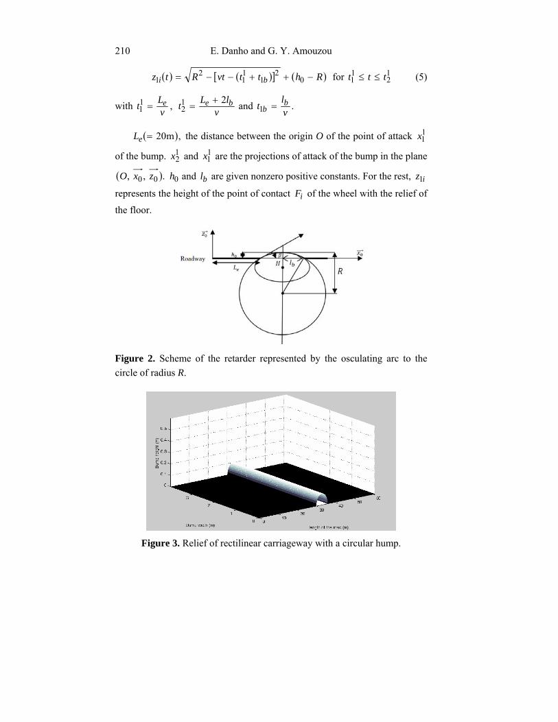
The relief of the floor. There are several types of floor models. In the case of a roadway that has a plurality of irregular locations, the floor can be modeled by a spectral density (PSD) [17-22]. In the case where the obstacle is isolated, the floor can be defined by a trigonometric function [4, 23], by a piecewise function [24] or modeled based on the characteristic function of the ellipse [9]. In this paper, the proposed model of terrain is circular as in [6] (Figure 2). Its equation is given by:

( ) ( )[ ] ( )RhlLxRxz be −++−−= 022 (3)

with R, the radius of the osculating circle to the bump that is defined according to the characteristics of the bump by:

.2 0

20

2

hhlR b +

= (4)

The shape of the carriageway which originates from the contact point of the front wheel with the floor is derived from equation (3) by:


( ) [ ( )] ( )RhttvtRtz bi −++−−= 02

111

21 for 1

211 ttt ≤≤ (5)

with ,11 v

Lt e= vlLt be 21

2+

= and .1 vlt b

b =

( ),m20=eL the distance between the origin O of the point of attack 11x

of the bump. 12x and 1

1x are the projections of attack of the bump in the plane

( ).,, 00 zxO 0h and bl are given nonzero positive constants. For the rest, iz1

represents the height of the point of contact iF of the wheel with the relief of

the floor.

Figure 2. Scheme of the retarder represented by the osculating arc to the circle of radius R.

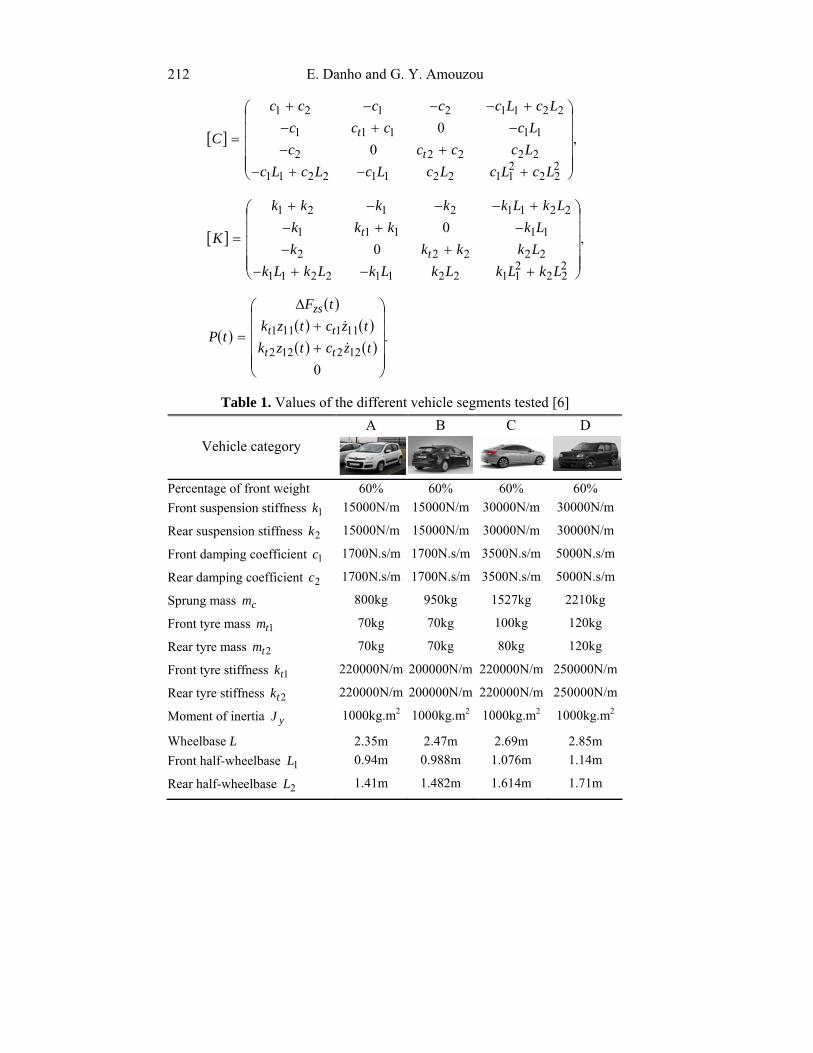
Figure 3. Relief of rectilinear carriageway with a circular hump.


2.2. Equations of motion

The equations of motion presented in this subsection are those from [9] with ( )tFzsΔ the extra effort specified in Section 3. The equations of the

motion around the equilibrium position are as follows:

( ) ( )

( ) ( ) ( )⎪⎩

⎪⎨⎧

Δ=ζ−ζ+ζ+ζ−ζ−ζ+

ζ−ζ+ζ+ζ−ζ−ζ+ζ

θθ

θθ

,222111

222111

tFLcLc

LkLkm

zszz

zzzb (6.a)

( ) ( )

( ) ( )⎪⎩

⎪⎨⎧

=ζ−θ−ζ+−ζ+

ζ−ζ−ζ−−ζ+ζ θ

,01111111

111111111

Lczc

Lkzkm

zt

ztt (6.b)

( ) ( )

( ) ( )⎪⎩

⎪⎨⎧

=ζ+ζ+ζ+−ζ+

ζ−ζ−ζ−−ζ+ζ

θ

θ

,02221222

222122222

Lczc

Lkzkm

zt

ztt (6.c)

( ) ( )

( ) ( )⎪⎩

⎪⎨⎧

=ζ−ζ+ζ+ζ−ζ−ζ−

ζ−ζ+ζ+ζ−ζ−ζ−ζ

θθ

θθθ

.022221111

22221111

LLcLLc

LLkLLkJ

zz

zzy (6.d)

These equations can be presented for better convenience in the following matrix form:

[ ] [ ] [ ] ( )[ ]tPKCM sss =ζ+ζ+ζ (7)

with [ ] 44×∈ RM the matrix of symmetric inertia, defined as positive .sζ∀

[ ] 44×∈ RC is the damping matrix, [ ] 44×∈ RK represents the stiffness

matrix and ( )[ ] 14×∈ RtP the vector of the forces applied to the system.

{ }θζζζζ∈ζ ;;; 21zs represents the vector of parameters about their

equilibrium positions. The structures of [ ],M [ ],C [ ]K and ( )tP are as

follows:

[ ] ,

000000000000

2

1

⎟⎟⎟⎟⎟

⎠

⎞

⎜⎜⎜⎜⎜

⎝

⎛

=

y

t

t

b

Jm

mm

M


[ ] ,0

0

222

21122112211

22222

11111

22112121

⎟⎟⎟⎟⎟

⎠

⎞

⎜⎜⎜⎜⎜

⎝

⎛

+−+−+−

−+−+−−−+

=

LcLcLcLcLcLcLccccLcccc

LcLccccc

Ct

t

[ ] ,0

0

222

21122112211

22222

11111

22112121

⎟⎟⎟⎟⎟

⎠

⎞

⎜⎜⎜⎜⎜

⎝

⎛

+−+−+−

−+−+−−−+

=

LkLkLkLkLkLkLkkkkLkkkk

LkLkkkkk

Kt

t

( )

( )( ) ( )( ) ( )

.

0122122

111111

⎟⎟⎟⎟⎟

⎠

⎞

⎜⎜⎜⎜⎜

⎝

⎛

++

Δ

=tzctzktzctzk

tF

tPtt

tt

zs

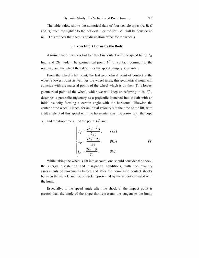
Table 1. Values of the different vehicle segments tested [6]

Vehicle category A

B C

D

Percentage of front weight 60% 60% 60% 60% Front suspension stiffness 1k 15000N/m 15000N/m 30000N/m 30000N/m

Rear suspension stiffness 2k 15000N/m 15000N/m 30000N/m 30000N/m

Front damping coefficient 1c 1700N.s/m 1700N.s/m 3500N.s/m 5000N.s/m

Rear damping coefficient 2c 1700N.s/m 1700N.s/m 3500N.s/m 5000N.s/m

Sprung mass cm 800kg 950kg 1527kg 2210kg

Front tyre mass 1tm 70kg 70kg 100kg 120kg

Rear tyre mass 2tm 70kg 70kg 80kg 120kg

Front tyre stiffness 1tk 220000N/m 200000N/m 220000N/m 250000N/m

Rear tyre stiffness 2tk 220000N/m 200000N/m 220000N/m 250000N/m

Moment of inertia yJ 1000kg.m2 1000kg.m2 1000kg.m2 1000kg.m2

Wheelbase L 2.35m 2.47m 2.69m 2.85m Front half-wheelbase 1L 0.94m 0.988m 1.076m 1.14m

Rear half-wheelbase 2L 1.41m 1.482m 1.614m 1.71m


The table below shows the numerical data of four vehicle types (A, B, C and D) from the lighter to the heaviest. For the rest, tic will be considered

null. This reflects that there is no dissipation effect for the wheels.

3. Extra Effort Borne by the Body

Assume that the wheels fail to lift off in contact with the speed hump 0h

high and bl2 wide. The geometrical point ∗iF of contact, common to the

roadway and the wheel then describes the speed bump type retarder.

From the wheel’s lift point, the last geometrical point of contact is the wheel’s lowest point as well. As the wheel turns, this geometrical point will coincide with the material points of the wheel which is up then. This lowest

geometrical point of the wheel, which we will keep on referring to as ,∗iF

describes a parabolic trajectory as a projectile launched into the air with an initial velocity forming a certain angle with the horizontal, likewise the center of the wheel. Hence, for an initial velocity v at the time of the lift, with a tilt angle β of this speed with the horizontal axis, the arrow ,fz the cope

px and the drop time pt of the point ∗iF are:

⎪⎪⎪

⎩

⎪⎪⎪

⎨

⎧

β=

β=

β=

)c.8(.sin2

)b.8(,2sin

)a.8(,2sin

0

0

20

22

gvt

gvx

gvz

p

p

f

(8)

While taking the wheel’s lift into account, one should consider the shock, the energy distribution and dissipation conditions, with the quantity assessments of movements before and after the non-elastic contact shocks between the vehicle and the obstacle represented by the asperity equated with the hump.

Especially, if the speed angle after the shock at the impact point is greater than the angle of the slope that represents the tangent to the hump


profile curve at that point, there will be a lift of the wheel. This will also depend on the tyre grip to the ground in that point and the intensity of the collision speed at that point, the state of the soil, the geometry of the retarder and the tyre tread and the dissipated or distributed energies.

Nevertheless, we can estimate a maximum speed and a maximum collision angle below which it is reasonably possible to consider that the lift does not occur.

To estimate the reasonable security area of non-lift, we assume that the

motion of ∗iF follows a parabolical trajectory at the most to the “limit” of lift

and non-lift which maximum height is 0h and the maximum drop distance is

.2 bl

Therefore, after we replaced fz and px by, respectively, 0h and bl2 in

(8.a) and (8.b) draw βsin2v from (8.b), and inject it in (8.a). We then get

the maximum angle maxβ that the velocity vector makes with the horizontal

axis of the roadway for which the wheels do not lift. Of course, beyond that angle, no conclusion can be drawn, since the wheels could lift or not. This angle is:

.2arctan 0max ⎟

⎠⎞

⎜⎝⎛=β

blh

(9)

Once maxβ is determined, then by equation (8.b), the maximum speed maxv

below which it can reasonably be said that the wheels do not lift is determined and its value is

.2arctan2sin

2

21

00

max⎪⎭

⎪⎬

⎫

⎪⎩

⎪⎨

⎧

⎥⎦⎤

⎢⎣⎡

⎟⎠⎞

⎜⎝⎛

=

b

b

lh

glv (10)

Beyond this speed, no conclusion can be drawn. The analyses must be supplemented by energetic studies. However, the numerical results are


subsequently used to estimate, for each geometry and each vehicle type, the speed range susceptible of being considered as thresholds for the actual lift.

In addition, we model ( )2 1 0, ,F F xξ = the angle that the longitudinal

axis of the vehicle forms with the flat part of the pavement by

.arctan21⎟⎠⎞

⎜⎝⎛

+=ξ LL

zni (11)

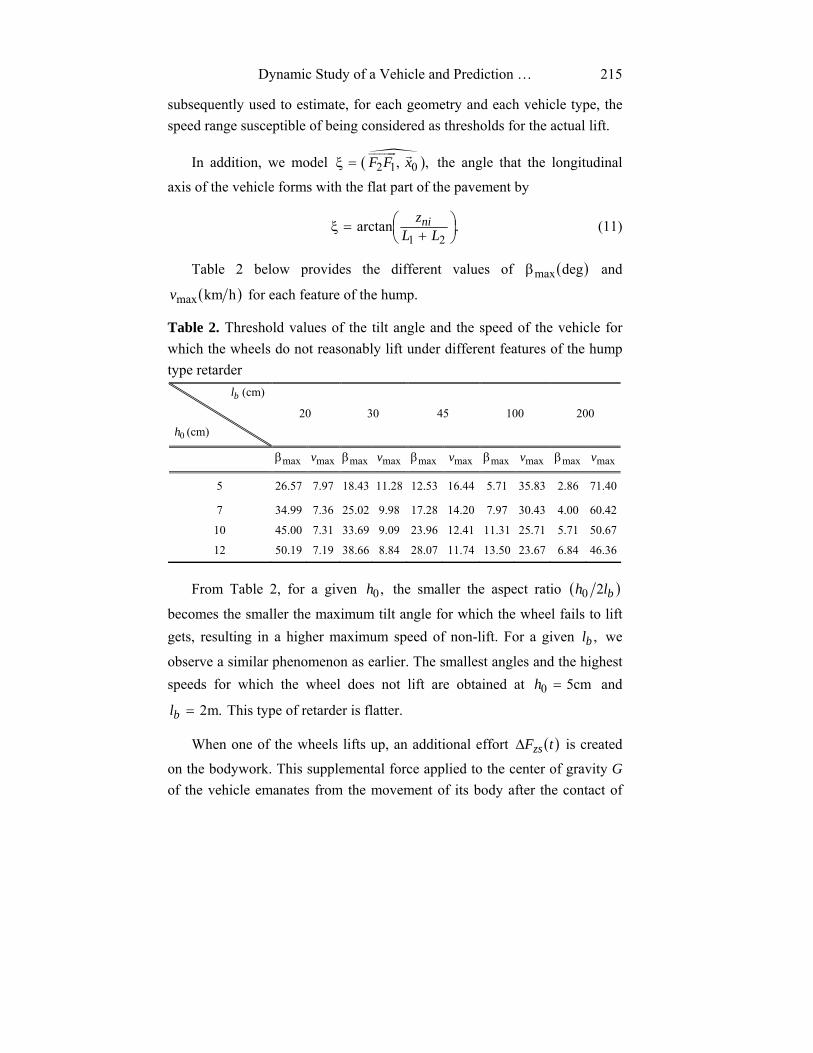
Table 2 below provides the different values of ( )degmaxβ and

( )hkmmaxv for each feature of the hump.

Table 2. Threshold values of the tilt angle and the speed of the vehicle for which the wheels do not reasonably lift under different features of the hump type retarder bl (cm)

0h (cm)

20 30 45 100 200

maxβ maxv maxβ maxv maxβ maxv maxβ maxv maxβ maxv

5 26.57 7.97 18.43 11.28 12.53 16.44 5.71 35.83 2.86 71.40

7 34.99 7.36 25.02 9.98 17.28 14.20 7.97 30.43 4.00 60.42

10 45.00 7.31 33.69 9.09 23.96 12.41 11.31 25.71 5.71 50.67

12 50.19 7.19 38.66 8.84 28.07 11.74 13.50 23.67 6.84 46.36

From Table 2, for a given ,0h the smaller the aspect ratio ( )blh 20

becomes the smaller the maximum tilt angle for which the wheel fails to lift gets, resulting in a higher maximum speed of non-lift. For a given ,bl we

observe a similar phenomenon as earlier. The smallest angles and the highest speeds for which the wheel does not lift are obtained at cm50 =h and

.m2=bl This type of retarder is flatter.

When one of the wheels lifts up, an additional effort ( )tFzsΔ is created

on the bodywork. This supplemental force applied to the center of gravity G of the vehicle emanates from the movement of its body after the contact of


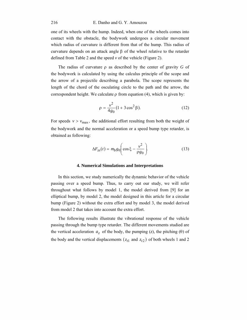
one of its wheels with the hump. Indeed, when one of the wheels comes into contact with the obstacle, the bodywork undergoes a circular movement which radius of curvature is different from that of the hump. This radius of curvature depends on an attack angle β of the wheel relative to the retarder defined from Table 2 and the speed v of the vehicle (Figure 2).

The radius of curvature ρ as described by the center of gravity G of the bodywork is calculated by using the calculus principle of the scope and the arrow of a projectile describing a parabola. The scope represents the length of the chord of the osculating circle to the path and the arrow, the correspondent height. We calculate ρ from equation (4), which is given by:

( ).cos3142

0

2β+=ρ g

v (12)

For speeds ,maxvv > the additional effort resulting from both the weight of

the bodywork and the normal acceleration or a speed bump type retarder, is obtained as following:

( ) .cos0

20 ⎟⎟

⎠

⎞⎜⎜⎝

⎛ρ

−ξ=Δ gvgmtF bzs (13)

4. Numerical Simulations and Interpretations

In this section, we study numerically the dynamic behavior of the vehicle passing over a speed bump. Thus, to carry out our study, we will refer throughout what follows by model 1, the model derived from [9] for an elliptical bump, by model 2, the model designed in this article for a circular bump (Figure 2) without the extra effort and by model 3, the model derived from model 2 that takes into account the extra effort.

The following results illustrate the vibrational response of the vehicle passing through the bump type retarder. The different movements studied are the vertical acceleration za of the body, the pumping (z), the pitching (θ) of

the body and the vertical displacements ( )21 and tt zz of both wheels 1 and 2


around their respective equilibrium position. In a first step, we compare the vertical accelerations of the body of model 3 with the works carried out in [6] (model 4). Then we compare the generalized coordinates for models 1 and 2 with those for models 2 and 3 for the vehicle A, model 3 is used to compare the vibrational behavior of vehicle bodies A, B, C and D. Finally, the behavior of the vehicle type B, for 0h set and type D for bl set, are studied

from model 3.

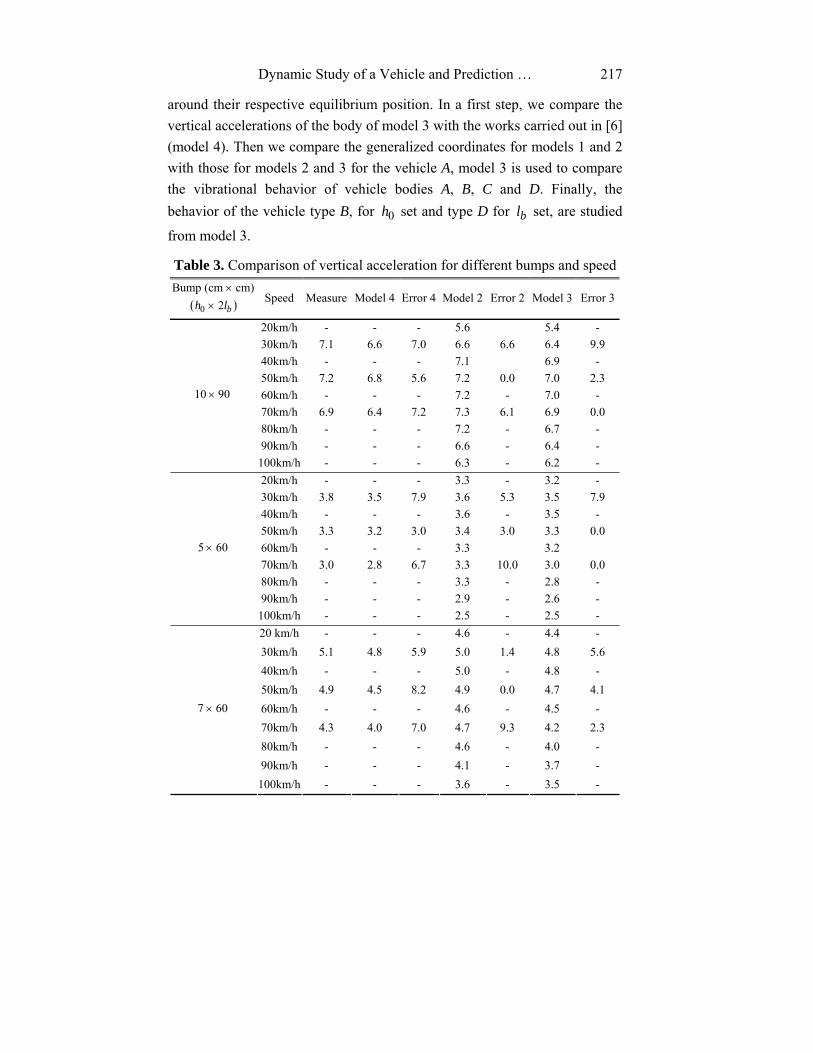
Table 3. Comparison of vertical acceleration for different bumps and speed Bump (cm × cm)

( )blh 20 × Speed Measure Model 4 Error 4 Model 2 Error 2 Model 3 Error 3

20km/h - - - 5.6 5.4 - 30km/h 7.1 6.6 7.0 6.6 6.6 6.4 9.9 40km/h - - - 7.1 6.9 - 50km/h 7.2 6.8 5.6 7.2 0.0 7.0 2.3 60km/h - - - 7.2 - 7.0 - 70km/h 6.9 6.4 7.2 7.3 6.1 6.9 0.0 80km/h - - - 7.2 - 6.7 - 90km/h - - - 6.6 - 6.4 -

9010 ×

100km/h - - - 6.3 - 6.2 - 20km/h - - - 3.3 - 3.2 - 30km/h 3.8 3.5 7.9 3.6 5.3 3.5 7.9 40km/h - - - 3.6 - 3.5 - 50km/h 3.3 3.2 3.0 3.4 3.0 3.3 0.0 60km/h - - - 3.3 3.2 70km/h 3.0 2.8 6.7 3.3 10.0 3.0 0.0 80km/h - - - 3.3 - 2.8 - 90km/h - - - 2.9 - 2.6 -

605 ×

100km/h - - - 2.5 - 2.5 - 20 km/h - - - 4.6 - 4.4 - 30km/h 5.1 4.8 5.9 5.0 1.4 4.8 5.6 40km/h - - - 5.0 - 4.8 - 50km/h 4.9 4.5 8.2 4.9 0.0 4.7 4.1 60km/h - - - 4.6 - 4.5 - 70km/h 4.3 4.0 7.0 4.7 9.3 4.2 2.3 80km/h - - - 4.6 - 4.0 - 90km/h - - - 4.1 - 3.7 -

607 ×

100km/h - - - 3.6 - 3.5 -


4.1. Comparison of the vertical acceleration of the vehicle C for different bumps and speeds (experimental validation)

The vertical acceleration, which reflects the discomfort of the driver and passengers is estimated and compared with experimental results in order to validate our model. Table 3 compares the vertical acceleration from models 2 and 3 with that of model 4 and measures.

From the results presented in this table, the relative errors calculated from model 2 (error 2) are significantly better than those calculated from model 4 (error 4) for the three characteristics of the retarder when speeds are below 70km/h. However, for the characteristics ( )cm602;cm50 == blh and

( )cm602;cm70 == blh of the bump at =v 70km/h, errors reach 10% for

model 2 against 7% for model 4. Errors calculated based on model 3, which takes into account the extra effort, are better than those calculated from Danho et al. model 2 when the speed exceeds a threshold that depends on the geometry of the bump. When the hump has a dimension of ( ),9010 × the

threshold is in the vicinity of 60km/h. By contrast, for a bump dimension of ( ),605 × the threshold is around 40km/h, while for a size ( ),607 × the speed

limit is still around 60km/h. Finally, we note that the higher the height of the bump increases, the higher the value of the threshold speed at which model 3 must be used rather than model 2 increases. In contrast, the larger the width of the bump, the lower the value of the threshold speed. In general, we observe an increase in the threshold speed with the appearance ratio of the bump .20 blh

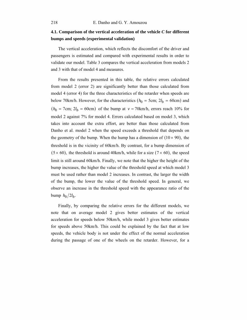
Finally, by comparing the relative errors for the different models, we note that on average model 2 gives better estimates of the vertical acceleration for speeds below 50km/h, while model 3 gives better estimates for speeds above 50km/h. This could be explained by the fact that at low speeds, the vehicle body is not under the effect of the normal acceleration during the passage of one of the wheels on the retarder. However, for a


slightly higher speed, this should be taken into account. Speed of 50km/h could be a threshold speed limit for both models (2 and 3) when the aspect ratio of the bump blh 20 is about .101 This threshold speed exceeds 50km/h

when 10120 >blh and it is lower than 50km/h when .10120 <blh

4.2. Compared study of the behavior of a type A vehicle by models 1 and 2

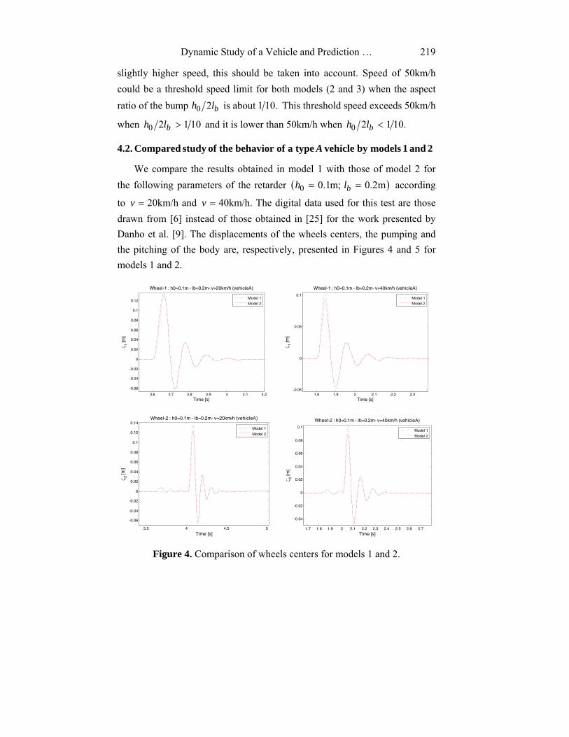
We compare the results obtained in model 1 with those of model 2 for the following parameters of the retarder ( )m2.0;m1.00 == blh according

to =v 20km/h and =v 40km/h. The digital data used for this test are those drawn from [6] instead of those obtained in [25] for the work presented by Danho et al. [9]. The displacements of the wheels centers, the pumping and the pitching of the body are, respectively, presented in Figures 4 and 5 for models 1 and 2.

3.6 3.7 3.8 3.9 4 4.1 4.2

-0.06

-0.04

-0.02

0

0.02

0.04

0.06

0.08

0.1

0.12

Time [s]

ζ 1 [m

]

Wheel-1 : h0=0.1m - lb=0.2m- v=20km/h (vehicleA)

Model 1

Model 2

1.8 1.9 2 2.1 2.2 2.3

-0.05

0

0.05

0.1

Time [s]

ζ 1 [m

]Wheel-1 : h0=0.1m - lb=0.2m- v=40km/h (vehicleA)

Model 1

Model 2

3.5 4 4.5 5

-0.06

-0.04

-0.02

0

0.02

0.04

0.06

0.08

0.1

0.12

0.14

Time [s]

ζ 2 [m

]


Model 1

Model 2

1.7 1.8 1.9 2 2.1 2.2 2.3 2.4 2.5 2.6 2.7

-0.04

-0.02

0

0.02

0.04

0.06

0.08

0.1

Time [s]

ζ 2 [m

]


Model 1

Model 2

Figure 4. Comparison of wheels centers for models 1 and 2.


3.5 4 4.5 5 5.5 6 6.5 7

-5

0

5

10

15

x 10-3

Time [s]

ζ z [m

]

Pumping : h0=0.1m - lb=0.2m- v=20km/h (vehicleA)

Model 1

Model 2

1.5 2 2.5 3 3.5 4 4.5

-5

0

5

10

15x 10

-3

Time [s]

ζ z [m

]


Model 1

Model 2

3.5 4 4.5 5 5.5 6 6.5

-0.6

-0.4

-0.2

0

0.2

0.4

0.6

0.8

1

Time [s]

ζ θ [d

eg]

Pitching : h0=0.1m - lb=0.2m- v=20km/h (vehicleA)

Model 1

Model 2

1.5 2 2.5 3 3.5 4

-0.4

-0.3

-0.2

-0.1

0

0.1

0.2

0.3

Time [s]

ζ θ [d

eg]


Model 1

Model 2

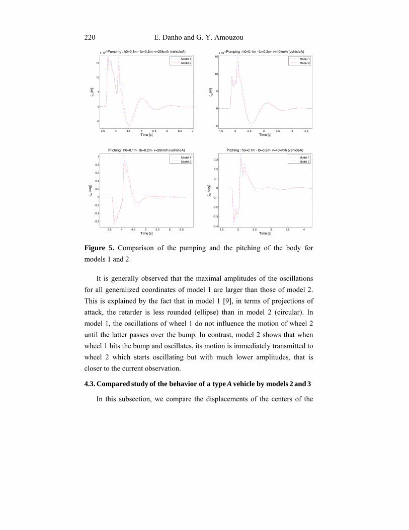
Figure 5. Comparison of the pumping and the pitching of the body for models 1 and 2.

It is generally observed that the maximal amplitudes of the oscillations for all generalized coordinates of model 1 are larger than those of model 2. This is explained by the fact that in model 1 [9], in terms of projections of attack, the retarder is less rounded (ellipse) than in model 2 (circular). In model 1, the oscillations of wheel 1 do not influence the motion of wheel 2 until the latter passes over the bump. In contrast, model 2 shows that when wheel 1 hits the bump and oscillates, its motion is immediately transmitted to wheel 2 which starts oscillating but with much lower amplitudes, that is closer to the current observation.

4.3. Compared study of the behavior of a type A vehicle by models 2 and 3

In this subsection, we compare the displacements of the centers of the


front and rear wheels as well as the pumping and the pitching of the body of a type A vehicle for models 2 and 3 (Figures 6 and 7).

2.4 2.6 2.8 3 3.2 3.4 3.6 3.8 4-0.04

-0.02

0

0.02

0.04

0.06

0.08

0.1

0.12

0.14

Time [s]

ζ 1 [m

]


Model 2

Model 3

1.4 1.5 1.6 1.7 1.8 1.9 2 2.1

-0.06

-0.04

-0.02

0

0.02

0.04

0.06

0.08

0.1

0.12

Time [s]

ζ 1 [m

]


Model 2

Model 3

2.8 3 3.2 3.4 3.6 3.8 4 4.2

-0.02

0

0.02

0.04

0.06

0.08

0.1

0.12

Time [s]

ζ 2 [m

]


Model 2

Model 3

1.3 1.4 1.5 1.6 1.7 1.8 1.9 2 2.1 2.2 2.3

-0.06

-0.04

-0.02

0

0.02

0.04

0.06

0.08

0.1

0.12

Time [s]

ζ 2 [m

]


Model 2

Model 3

Figure 6. Comparison of wheels displacements for models 2 and 3.

We observe that the curves of the vertical displacements of the wheels centers for models 2 and 3 are almost identical (Figure 6). The unsprung mass is not hence influenced by the inclusion of the extra effort. Indeed, this force acts on the sprung mass (the body) so that the vehicle sways a little more for model 2 than for model 3. Pumping amplitudes for model 3 are much larger than those of model 2 and decrease with speed (Figure 7).


2 3 4 5 6 7 8

-0.01

0

0.01

0.02

0.03

0.04

Time [s]

ζ z [m

]


Model 2

Model 3

1.5 2 2.5 3 3.5 4 4.5 5

-0.01

-0.005

0

0.005

0.01

0.015

0.02

0.025

0.03

0.035

Time [s]

ζ z [m

]


Model 2

Model 3

2.5 3 3.5 4 4.5 5 5.5

-1

-0.8

-0.6

-0.4

-0.2

0

0.2

0.4

0.6

0.8

1

Time [s]

ζ θ [d

eg]


Model 2

Model 3

1 1.5 2 2.5 3 3.5 4 4.5 5 5.5

-0.5

-0.4

-0.3

-0.2

-0.1

0

0.1

0.2

0.3

0.4

Time [s]

ζ θ [d

eg]


Model 2

Model 3

Figure 7. Comparison of the body movement for models 2 and 3.

4.4. Vehicle behavior for the four types of vehicle

In this paragraph, we compare the vibrational motion of the body and the wheels for four different categories (A, B, C and D) of vehicles for =v 15km/h and 30km/h (Figures 8 and 9). It is generally observed that the

oscillations experienced by the different vehicles increase with the speed. Furthermore, there is a phase shift between oscillations from one vehicle to another. This reflects the dissimilarity of the vehicles front wheelbases. Indeed, the front wheelbase increases from vehicle A to vehicle D. Thus, the larger it is, the sooner the vehicle is disrupted. Moreover, we note, considering the oscillation resulting from the first contact of the wheel with the bump, that the lighter the vehicle, the greater the amplitude.


4.8 5 5.2 5.4 5.6 5.8 6 6.2 6.4

0

0.02

0.04

0.06

0.08

0.1

Time [s]

ζ 1 [m

]

Wheel-1 : h0=0.1m - lb=0.45m- v=15km/h

Type AType B

Type CType D

2.3 2.4 2.5 2.6 2.7 2.8 2.9 3 3.1 3.2

-0.04

-0.02

0

0.02

0.04

0.06

0.08

0.1

0.12

Time [s]

ζ 1 [m

]

Wheel-1 : h0=0.1m - lb=0.45m- v=30km/h

Type AType B

Type CType D

5 5.5 6 6.5 7

-0.02

0

0.02

0.04

0.06

0.08

0.1

Time [s]

ζ 2 [m

]

Wheel-2 : h0=0.1m - lb=0.45m- v=15km/h

Type AType B

Type CType D

2.4 2.5 2.6 2.7 2.8 2.9 3 3.1 3.2 3.3

-0.04

-0.02

0

0.02

0.04

0.06

0.08

0.1

0.12

Time [s]

ζ 2 [m

]

Wheel-2 : h0=0.1m - lb=0.45m- v=30km/h

Type AType B

Type CType D

Figure 8. Comparison of wheels vertical displacements for four vehicles types.


4.5 5 5.5 6 6.5 7 7.5 8 8.5

-0.01

0

0.01

0.02

0.03

0.04

0.05

0.06

0.07

Time [s]

ζ z [m

]

Pumping : h0=0.1m - lb=0.45m- v=15km/h

Type AType B

Type CType D

2.5 3 3.5 4 4.5 5 5.5

-0.01

0

0.01

0.02

0.03

0.04

0.05

Time [s]

ζ z [m

]

Pumping : h0=0.1m - lb=0.45m- v=30km/h

Type AType B

Type CType D

4.5 5 5.5 6 6.5 7

-1.5

-1

-0.5

0

0.5

1

1.5

2

Time [s]

ζ θ [d

eg]

Pitching : h0=0.1m - lb=0.45m- v=15km/h

Type AType B

Type CType D

2.5 3 3.5 4 4.5

-1

-0.5

0

0.5

1

1.5

Time [s]

ζ θ [d

eg]

Pitching : h0=0.1m - lb=0.45m- v=30km/h

Type AType B

Type CType D

Figure 9. Comparison of the pumping and the pitching of the body for four types of vehicles.

4.5. Influence of the geometry of the retarder on the vehicle behavior

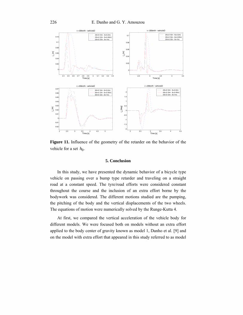
In this paragraph, we investigate the influence of the relief of the retarder on the dynamic behavior of two vehicles (B and D) (Figures 10 and 11). We note that, conformably to the predictions obtained in our first study [9], the amplitudes of the oscillations of the different motions increase when increasing the bump height at fixed-width ((0.05m; 0.45m), (0.1m; 0.45m) and (0.12m; 0.45m)), i.e., when the aspect ratio of the bump increases. In addition, when the bump is spread at fixed height ((0.12m; 0.2m), (0.12m; 0.45m) and (0.12m; 1m)), the path traveled by wheel 1 to the summit becomes lengthier. Thus, the position of the center of gravity remains high for longer. The maximum amplitude of the pumping and pitching is reached


when wheel 1 is at the top of the hump and the minimum amplitude is achieved when wheel 2 reaches the top of the hump (Figure 11). Moreover, the pumping and the pitching minimal amplitudes decrease with the width of the hump at fixed height, i.e., the lower the aspect ratio of the bump, the less discomfort the passenger felt. The crushing of the body is then maximal.

2.4 2.5 2.6 2.7 2.8 2.9 3

-0.05

0

0.05

0.1

0.15

Time [s]

ζ 1 [m

]

v =30km/h - vehicleB

(h0=0.05m - lb=0.45m)

(h0=0.1m - lb=0.45m)(h0=0.12m - lb=0.45m)

2.4 2.5 2.6 2.7 2.8 2.9 3 3.1 3.2 3.3 3.4

-0.06

-0.04

-0.02

0

0.02

0.04

0.06

0.08

0.1

0.12

0.14

Time [s]

ζ 2 [m

]


(h0=0.05m - lb=0.45m)

(h0=0.1m - lb=0.45m)(h0=0.12m - lb=0.45m)

2.5 3 3.5 4 4.5 5 5.5 6

-0.02

-0.01

0

0.01

0.02

0.03

0.04

0.05

0.06

Time [s]

ζ z [m

]


(h0=0.05m - lb=0.45m)

(h0=0.1m - lb=0.45m)(h0=0.12m - lb=0.45m)

2.5 3 3.5 4 4.5 5 5.5 6

-1

-0.8

-0.6

-0.4

-0.2

0

0.2

0.4

0.6

0.8

Time [s]

ζ θ [d

eg]


(h0=0.05m - lb=0.45m)

(h0=0.1m - lb=0.45m)(h0=0.12m - lb=0.45m)

Figure 10. Influence of the geometry of the retarder on the vehicle behavior for a set .lb


2.4 2.5 2.6 2.7 2.8 2.9 3 3.1 3.2 3.3 3.4

0

0.02

0.04

0.06

0.08

0.1

0.12

Time [s]

ζ 1 [m

]

v =30km/h - vehicleD

(h0=0.12m - lb=0.2m)

(h0=0.12m - lb=0.45m)(h0=0.12m - lb=1m)

2.5 3 3.5 4 4.5

0

0.02

0.04

0.06

0.08

0.1

Time [s]

ζ 2 [m

]


(h0=0.12m - lb=0.2m)

(h0=0.12m - lb=0.45m)(h0=0.12m - lb=1m)

2 2.5 3 3.5 4 4.5 5

-0.02

-0.01

0

0.01

0.02

0.03

0.04

0.05

0.06

0.07

Time [s]

ζ z [m

]


(h0=0.12m - lb=0.2m)

(h0=0.12m - lb=0.45m)(h0=0.12m - lb=1m)

2 2.5 3 3.5 4 4.5

-2

-1.5

-1

-0.5

0

0.5

1

1.5

2

Time [s]

ζ θ [d

eg]


(h0=0.12m - lb=0.2m)

(h0=0.12m - lb=0.45m)(h0=0.12m - lb=1m)

Figure 11. Influence of the geometry of the retarder on the behavior of the vehicle for a set .0h

5. Conclusion

In this study, we have presented the dynamic behavior of a bicycle type vehicle on passing over a bump type retarder and traveling on a straight road at a constant speed. The tyre/road efforts were considered constant throughout the course and the inclusion of an extra effort borne by the bodywork was considered. The different motions studied are the pumping, the pitching of the body and the vertical displacements of the two wheels. The equations of motion were numerically solved by the Runge-Kutta 4.

At first, we compared the vertical acceleration of the vehicle body for different models. We were focused both on models without an extra effort applied to the body center of gravity known as model 1, Danho et al. [9] and on the model with extra effort that appeared in this study referred to as model


2. We compared the conclusions reached by these models with those proposed by Garcia-Pozuelo et al. [6] in model 4 and with experimental measures to validate these results. The generalized coordinates for model 1 and those for models 2 and 3 for a given vehicle were compared, as well. Next, we carried out a comparative study of the vibrational behavior of the body for four types of vehicles. Finally, the influence of the geometry of the retarder on the vehicle behavior has been investigated. Simulations performed show that the predicted estimates on the body vertical acceleration are overall better than for speeds above 50km/h when we take into account the load transfer type extra effort at the level of the body center of gravity. In contrast, for low speeds, i.e., less than 50km/h, the body does not take off enough and therefore is not influenced by a normal acceleration. At this level, estimates of vertical acceleration are thus best when models that disregard this new effort are used. Furthermore, the more the height of the bump increases, the more the threshold speed value at which model 3 must be used rather than model 2 rises. On the other hand, the more the width of the bump increases, the more the threshold speed value decreases. Generally, the threshold speed increases with the aspect ratio blh 20 of the body. For

,10120 >blh the threshold speed is above 50km/h and it is less than

50km/h when .10120 <blh The speed of 50km/h could be a threshold

speed limit for models 2 and 3 when the aspect ratio of the bump blh 20 is

about .101 We also notice that the oscillations of the different vehicles

increase with the speed and with a phase shift from one vehicle to another due to the difference of wheelbase between vehicles. Furthermore, the amplitude of the first oscillations increases with the vehicle mass. The analysis of the influence of the retarder geometry on two types of vehicles revealed that identically to Danho et al.’s work [9], the amplitudes of the oscillations of the different movements increase with the bump aspect ratio. Finally, the maximum amplitudes of the body motion are reached when the front wheel is on top of the hump whereas the minimum amplitudes are obtained when the rear wheel reaches the top of the bump. The lower the aspect ratio of the bump, the less the discomfort felt by the passengers.


References

[1] C. E. T. E. De l’Ouest, Surélévations de chaussée: outils de modération des vitesses, Décembre 2010.

[2] E. Khorshid and M. Alfares, A numerical study on the optimal geometric design of speed control humps, Eng. Optim. 36(1) (2004), 77-100.

[3] D. E. Clark, All-way stops versus speed humps: which is more effective at slowing traffic speeds? ITE Annual Meeting Compendium, 2000.

[4] T. A. O. Salau, A. O. Adeyefa and S. A. Oke, Vehicle speed control using road bumps, Transport 19(3) (2004), 130-136.

[5] S. Aslan, O. Karcioglu, Y. Katirci, H. Kandiş, N. Ezirmik and O. Bilir, Speed bump-induced spinal column injury, The American Journal of Emergency Medicine 23(4) (2005), 563-564.

[6] D. Garcia-Pozuelo, A. Gauchia, E. Olmeda and V. Diaz, Bump modeling and vehicle vertical dynamics prediction, Advances in Mechanical Engineering 2014 (2014), Article ID 736576, 10 pp.

[7] M. Pau and S. Angius, Do speed bumps really decrease traffic speed? An Italian experience, Accident Analysis and Prevention 33(5) (2001), 585-597.

[8] S. Aslan, O. Karcioglu, Y. Katirci, H. Kandiş, N. Ezirmik, and O. Bilir, Speed bump-induced spinal column injury, The American Journal of Emergency Medicine 23(4) (2005), 563-564.

[9] E. Danho, G. Y. Amouzou, N. R. Djué, J. M. Zokagoa, K. K. S. Yanga and N. Coulibaly, Dynamic behavior of a vehicle on a pavement with series of speed bumps type checks, Far East J. Appl. Math. 82(2) (2013), 101-122.

[10] W. F. Milliken and D. L. Milliken, Race car vehicle dynamics, SAE Int., Warrendale, PA, US, 1995, pp. 473-480.

[11] B. Badji, Caractérisation du comportement non linéaire en dynamique du véhicule, Thèse de Doctorat (Ph.D.), Université de Technologie de Belfort-Montbeliard, 2009.

[12] D. Lechner, Analyse du comportement dynamique des véhicules routiers légers: développement d’une méthodologie appliquée à la sécurité primaire, Thèse de Doctorat (Ph.D.), Ecole Centrale de Lyon, France, 2002.

[13] E. Velenis, P. Tsiotras, C. Canudas-De-Wit and M. Sorine, Dynamic tyre friction models for combined longitudinal and lateral vehicle motion, Vehicle System Dynamics 43(1) (2005), 3-29.


[14] M. Sharifi and B. Shahriari, Pareto optimization of vehicle suspension vibration for a nonlinear half-car model using a multi-objective genetic algorithm, Res. J. Recent Sci. 1(8) (2012), 17-22.

[15] J. J. Martinez-Molina, J. C. Avila-Vilchis and C. Canudas-de-Wit, A new bicycle vehicle model with dynamic contact friction, IFAC Symposium on “Advances in Automotive Control”, University of Salerno, Italy, April 19-23, 2004.

[16] V. Harth, M. Fayet, L. Maiffredy and C. Renou, A modelling approach to tire-obstacle interaction, Multibody System Dynamics 11(1) (2004), 23-39.

[17] B. R. Davis and A. G. Thompson, Power spectral density of road profiles, Vehicle System Dynamics 35(6) (2001), 409-415.

[18] ISO-8608, Mechanical vibration-road surface profiles-reporting of measured data, 1995.

[19] M. Bouazara, Étude et analyse de la suspension active et semi active des véhicules routiers, Thèse de Doctorat (Ph.D.), Québec/Université Laval/164p, 1997.

[20] J. D. Robson, Road surface description and vehicle response, International Journal of Vehicle Design 1 (1979), 25-35.

[21] C. J. Dodds and J. D. Robson, The description of road surface roughness, J. Sound Vibration 31(2) (1973), 175-183.

[22] O. Kropáč and P. Múčka, Effect of obstacles on roads with different waviness values on the vehicle response, Vehicle System Dynamics 46(3) (2008), 155-178.

[23] D. Sekulić, V. Dedović and S. Rusov, Effect of shock vibrations due to speed control humps to the health of city bus drivers, Scientific Research and Essays 7(5) (2012), 573-585.

[24] G. Lombaert, G. Degrande and D. Clouteau, Numerical modelling of free field traffic-induced vibrations, Soil Dynamics and Earthquake Engineering 19(7) (2000), 473-488.

[25] E. Esmailzadeh and N. Jalili, Vehicle-passenger-structure interaction of uniform bridges traversed by moving vehicles, J. Sound Vibration 260(4) (2003), 611-635.

dynamic study of a vehicle and prediction of its …

Documents