dynamic stochastic models for decision making under time constraints

File: 480J 116701 . By:DS . Date:17:09:97 . Time:09:31 LOP8M. V8.0. Page 01:01Codes: 6387 Signs: 4743 . Length: 60 pic 11 pts, 257 mm

Journal of Mathematical Psychology � MP1167

journal of mathematical psychology 41, 260�274 (1997)

Dynamic Stochastic Models for DecisionMaking under Time Constraints

Adele Diederich

C.v. Ossietzky Universita� t, Oldenburg, Germany

This paper introduces the multiattribute dynamic decision model(MADD) to describe both the dynamic and the stochastic nature ofdecision making. MADD is based on information processing modelsdeveloped by Diederich. It belongs to the class of sequentialcomparison models and generalizes and extends the so-called decisionfield theory (DFT) of Busemeyer and Townsend. Describing thedecision maker's choice behavior for multiattribute choice alternativesin an uncertain environment by a stochastic process, the Ornstein�Uhlenbeck process, MADD predicts choice probabilities and meanchoice response times when the decision maker has to respond withina given time limit. This paper outlines the prediction of two differentversions of the model in detail. ] 1997 Academic Press

1. INTRODUCTION

Investigating decision making under time constraintshas become increasingly popular over the last decades.(Recently, an entire book was devoted to this subject,Svenson and Maule, 1993.) Two theoretical approaches canbe distinguished among the predominantly experimentallyguided research efforts:

(a) According to one approach, the decision makerpossesses a collection of different decision strategies andchooses one depending on the choice situation. Theoriesdiffer with respect to situation�person determinants forselecting a strategy. The cost�benefit approach (Beach 6Mitchell, 1978; Payne, Bettman, 6 Johnson, 1988) assumesthat decision strategies can be distinguished in terms of theiraccuracy and cognitive effort. The selection of a decisionstrategy is seen as a compromise between maximizingaccuracy and minimizing effort. Under time constraints, thedecision maker is forced to select a strategy that is less timeconsuming but also less accurate. Janis and Mann (1977)assume that emotional factors and stress factors influencethe selection of a decision strategy. Time constraintsinducing stress lead to the adoption of less effective decision

strategies. For a review of other studies and findings seeEdland and Svenson (1993). I call these models decisionrule (strategy) selection models. Test of the cost�benefitapproaches usually involve choices among two or morealternatives.

(b) According to the other approach, the decisionmaker considers features of choice alternatives sequentiallyover time. Each feature comparison results in a value, whichis integrated with the other values, producing a preferencestate at each moment in time. The preference moves ina random walk manner until a preset decision criterion(or decision boundary), characteristic for each choicealternative, is reached. At that point the process stops anda decision is made. These models are called sequentialcomparison models (Albert, Aschenbrenner, 6 Schmalhofer,1988; Aschenbrenner, Albert, 6 Schmalhofer, 1984;Busemeyer, 1985; Busemeyer 6 Townsend, 1992, 1993;Diederich, 1995b; Wallsten 6 Barton, 1982, forprobabilistic inference). The main difference among thesemodels is how information about the choice alternatives isselected, evaluated, and integrated with the evaluations.Within these approaches, setting the decision maker undertime pressure changes the decision maker's criterion ratherthan changing her or his strategies. The criterion is anincreasing function of the time available for a decision. Testsof these models usually involve binary choices.

Sequential comparison models explicitly model the timeit takes to reach a decision and, therefore, they naturallyyield predictions for decision making under time con-straints.

In the following, I present a dynamic stochastic decisionmodel for binary multiattribute decision problems, calledmultiattribute dynamic decision model (MADD). MADDis a sequential comparison model and it extends andgeneralizes the so-called decision field theory (DFT) byBusemeyer and Townsend (1992, 1993) which applies tounidimensional choice alternatives.

First, I describe the model according to its assumptionsabout information selection, evaluation, and integration, aswell as about how the process terminates. Then, I present amathematical development of the model, followed by

article no. MP971167

2600022-2496�97 �25.00

Copyright � 1997 by Academic PressAll rights of reproduction in any form reserved.

Correspondence and reprint requests should be addressed to AdeleDiederich, C.v. Ossietzky Universita� t, Institut fu� r Kognitionsforschung,FB 5, Psychologie, A6, D-26111 Oldenburg, Germany. E-mail: diederich�psychologie.uni-oldenburg.de.

File: 480J 116702 . By:SD . Date:05:09:97 . Time:08:54 LOP8M. V8.0. Page 01:01Codes: 6257 Signs: 5265 . Length: 56 pic 0 pts, 236 mm

specific assumptions about the composition of the delibera-tion process. In this paper I particularly focus on MADD'spredictions with respect to decision making under timeconstraints.

2. MULTIATTRIBUTE DYNAMIC DECISION MODEL

Choice alternatives in multiattribute decision problemsare usually characterized by attributes and by specific valuesfor each attribute. These values are mapped on a scalespecified in the particular research area (for example, utility,Keeny and Raiffa, 1976; attractiveness, Aschenbrenner,Albert, 6 Schmalhofer, 1984; Montgomery 6 Svenson,1976; Svenson, 1979). Instead, MADD assumes that thedecision maker uses attributes as memory retrieval cues forconcrete ideas and aspects about the choice objects. Thedecision maker tries to anticipate and evaluate all possibleconsequences produced by choosing either of the alter-natives. The anticipated consequences are retrieved from acomplex associative memory process and it takes time toretrieve, compare and integrate the comparisons. Thedeliberation process might be accompanied by conflict anddoubts. Obviously it is not possible to describe or predictthis deliberation process in any detail. Rather, the goal ofthe model presented below is to understand the maincognitive mechanisms that guide the deliberation processthat is involved in decisions made under uncertainty.

2.1. Information Selection

When confronted with a choice problem the decisionmaker draws the information about the alternatives fromhis or her memory. The possible consequences connectedwith choosing either of the alternatives are learned fromexperience and the decision maker remembers them more orless well. The decision maker considers attributes the alter-natives may or may not have in common. Assume theattribute that comes first to the decision maker's mind willbe processed first. This attribute might be the most impor-tant or the most salient one for the decision maker (seeAschenbrenner et al., 1984; Wallsten 6 Barton, 1982). Thedecision maker may reconsider attributes several times.

2.2. Evaluation and Integration

A preference state is activated as soon as the decisionmaker is confronted with a decision problem and startsthinking about an attribute. The process is modelled asa continuous-time stochastic process. The variable, t,represents the amount of time that has elapsed since thedecision maker has been confronted with the decisionproblem. At each point in time, the decision maker has anew preference state, denoted by Xt . Positive values, Xt>0,indicate a momentary preference for alternative A, say,

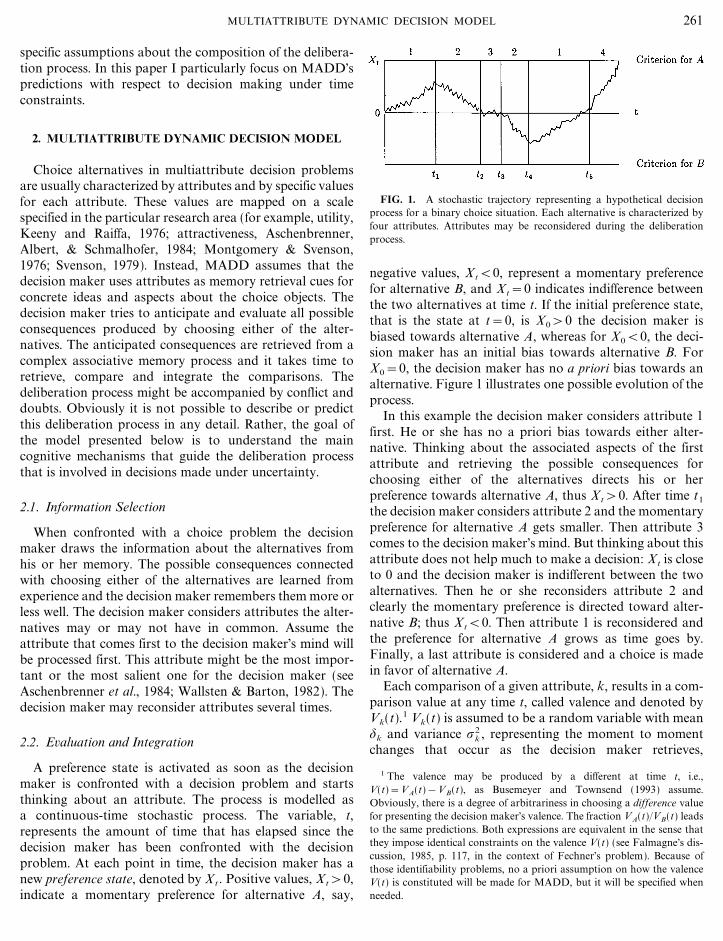
FIG. 1. A stochastic trajectory representing a hypothetical decisionprocess for a binary choice situation. Each alternative is characterized byfour attributes. Attributes may be reconsidered during the deliberationprocess.

negative values, Xt<0, represent a momentary preferencefor alternative B, and Xt=0 indicates indifference betweenthe two alternatives at time t. If the initial preference state,that is the state at t=0, is X0>0 the decision maker isbiased towards alternative A, whereas for X0<0, the deci-sion maker has an initial bias towards alternative B. ForX0=0, the decision maker has no a priori bias towards analternative. Figure 1 illustrates one possible evolution of theprocess.

In this example the decision maker considers attribute 1first. He or she has no a priori bias towards either alter-native. Thinking about the associated aspects of the firstattribute and retrieving the possible consequences forchoosing either of the alternatives directs his or herpreference towards alternative A, thus Xt>0. After time t1

the decision maker considers attribute 2 and the momentarypreference for alternative A gets smaller. Then attribute 3comes to the decision maker's mind. But thinking about thisattribute does not help much to make a decision: Xt is closeto 0 and the decision maker is indifferent between the twoalternatives. Then he or she reconsiders attribute 2 andclearly the momentary preference is directed toward alter-native B; thus Xt<0. Then attribute 1 is reconsidered andthe preference for alternative A grows as time goes by.Finally, a last attribute is considered and a choice is madein favor of alternative A.

Each comparison of a given attribute, k, results in a com-parison value at any time t, called valence and denoted byVk(t).1 Vk(t) is assumed to be a random variable with mean$k and variance _2

k , representing the moment to momentchanges that occur as the decision maker retrieves,

261MULTIATTRIBUTE DYNAMIC DECISION MODEL

1 The valence may be produced by a different at time t, i.e.,V(t)=VA(t)&VB(t), as Busemeyer and Townsend (1993) assume.Obviously, there is a degree of arbitrariness in choosing a difference valuefor presenting the decision maker's valence. The fraction VA(t)�VB(t) leadsto the same predictions. Both expressions are equivalent in the sense thatthey impose identical constraints on the valence V(t) (see Falmagne's dis-cussion, 1985, p. 117, in the context of Fechner's problem). Because ofthose identifiability problems, no a priori assumption on how the valenceV(t) is constituted will be made for MADD, but it will be specified whenneeded.


evaluates, and compares the values of the attributes, andconsiders possible consequences for choosing either of thealternatives. The valence Vk(t) at time t is integrated withthe previous preference state Xt , resulting in a newpreference state Xt+{ at time t+{, where { is a very smallamount of time. The new preference state Xt+{ is defined as

Xt+{=(1&#k{)Xt+{Vk (t). (1)

(1&#k{) weighs the previous preference state with respectto attribute k and { weighs the new valence value producinga new preference updated continuously over time.

2.3. Choice

It is assumed that the deliberation process continues untila preset decision criterion % is reached and a choice is made.That is, the preference state has to reach a value that is equalto or more extreme than the value of % before a decision canbe made. In this example, the decision maker chooses alter-native A as soon as Xt>%; alternative B is chosen as soonas &Xt>%.

The criterion is set by the decision maker when con-fronted with the choice task. It may depend on personalcharacteristics and�or on task and situation characteristics.For example, for an important decision, the decision makersets a high %, allowing him or her to accumulate moreevidence prior to choice. The criterion may also depend onthe available time for making a decision. That is, % isassumed to be smaller with, than without, time constraints.The criterion is assumed to be fixed within a choice situationbut may vary across choice situations.2

Note, that the preference state at any point in time is notobservable and not necessarily open to introspection and,therefore, the hypothetical deliberation process is notdirectly observable. Nevertheless, some properties of themodel seem obvious: the preference for alternative A and Bmay change during the deliberation process; the strength ofpreference may depend on the attribute; the order ofattributes the decision maker is thinking of may be crucialfor his or her decision; setting the decision maker under timepressure may reverse a decision. In order to elaborate thesefeatures of the model we now turn to its formal development.

3. MATHEMATICAL DEVELOPMENT OF MADD

The decision process representing the decision maker'spreference for alternatives A or B at any time t is describedby a continuous-time, continuous-state stochastic process,[Xt : t�0], Xt for short, with two absorbing boundaries,% and &%. The space state, S, in which the values x of therandom variable Xt lie, is assumed to consist of different

degrees of preference, called the preference states. Inparticular, I assume such a stochastic process (diffusionprocess) for each attribute k considered by the decisionmaker.

Each process I consider here is characterized by two coef-ficients, a drift coefficient +k(x)=$k&#kx and a diffusioncoefficient _2

k(x)=_2k .3 The drift coefficient determines the

direction and velocity of the process, the diffusion coefficientindicates the variance of the increments of the process.4

Here, $k represents the mean valence resulting from thecomparison between the alternatives A and B with respectto attribute k. Assuming the valence to be produced by thedifference of valences for A and B, then, without loss ofgenerality, $k>0 indicates a preference for alternative Awith respect to attribute k, say, and $k<0 indicates apreference for alternative B with respect to attribute k.Assuming instead the valence to be produced by the ratio ofthe valences for A and B, then $k>1 indicates a preferencefor alternative A, and $k<1 indicates a preference for alter-native B with respect to attribute k. The second part of thedrift coefficient, &#kx, indicates that the drift varies propor-tionally to the value of the process.5

The parameter #k which I call the conflict parameteraccounts for various conflict situations. #k>0 indicates anavoidance�avoidance conflict situation. That is, the weightof the previous preference state becomes smaller (see Eq. 1)and the increments of the process get increasingly smaller asthe distance from the starting position, i.e., from the initialpreference state at time t=0, becomes larger. This impliesthat it takes longer to reach a preset criterion. #k<0indicates an approach�approach conflict situation. That is,the weight of the previous preference state becomes largerand the increments of the process get increasingly larger asthe distance from the initial preference state increases andtherefore the process more quickly reaches a preset decisioncriterion. #k=0 indicates no conflict.6 With #k refering to aconflict with respect to attribute k, three different conflictsituations, i.e., approach�approach; avoidance�avoidance;and approach�avoidance, in the spirit of Lewin (1931,1951) and Miller (1944), can be accounted for; _2 accountsfor the moment-to-moment variability of evaluating thepossible outcomes.

262 ADELE DIEDERICH

2 Compare speed�accuracy trade-off.

3 A diffusion process with these specific drift and diffusion coefficients iscalled an Ornstein�Uhlenbeck process.

4 The increment of the process in the small time interval (t, t+{] isXt+{&Xt . The drift coefficient for a diffusion process, also calledinfinitesimal first moment or infinitesimal mean, is in general defined as+(x, t)=lim{ � 0 E[X(t+{)&X(t) | X(t)=x)]�{. The diffusion coefficient,also called infinitesimal second moment or infinitesimal variance, is ingeneral defined as _2(x, t)=lim{ � 0 E[X(t+{)&X(t) | X(t)=x)]�{.

5 In physics and biology this quantity reflects a restoring force directedto the origin, i.e., a force that pulls the process (particle) back to the origin.The force is larger as the distance from the origin increases.

6 Note, that with #=0 the Ornstein�Uhlenbeck process reduces to aWiener process with drift.


Note, while the diffusion coefficient is independent of thestate of preference, the drift changes with location x, i.e., theprocess does not have independent increments. Further, theprocess is time-homogeneous with respect to each singleattribute the decision maker considers.

The standard way to determine the choice probabilityand the mean choice response time for diffusion processmodels is to solve a partial differential equation, theKolmogorov backward equation. Unfortunately, no closedform solution is known for the Ornstein�Uhlenbeckprocess with absorbing boundaries (Ricciardi, 1977, p. 128;Bhattacharya 6 Waymire, 1990, p. 389). Therefore, abirth�death chain, a discrete-time discrete-state stochasticprocess, for which solutions exist, is used to approximatethe Ornstein�Uhlenbeck diffusion process, which is acontinuous-time, continuous-state stochastic process. Thederivations for this procedure can be found in Appendix A.

3.1. Choice Probability and Mean Choice Response Time

Next the probability to choose an alternative and the timeit takes to decide, both interpreted as preference strength,have to be determined. That is, the probability that the pro-cess eventually reaches one of the boundaries of the process(the criterion to decide for one alternative) for the first time,the first passage probability, has to be calculated. Moreover,the time taken by the process to go to one of the boundariesfor the first time, the first passage time, has to be deter-mined. The decision criteria or boundaries of the process areabsorbing states7 of the process, since once the decisionprocess reaches a criterion a decision is made and theprocess is absorbed. The transition probability densityp(t ; x, y) of the diffusion process is approximated by trans-ition probabilities p (n)

ij of the birth�death chain the trans-ition probability matrix P for that chain has to be deter-mined.

The state space of the process, S, is defined as the set ofstates of preference for the decision process. Assume that thepreference changes by very small steps of size 2 (see alsoAppendix A). Then, the total number of preference statescan be expressed as a function of the step size 2 and thecriterion % by setting %=l2. Consequently S equals

S=[0, \2, \22, \ } } } \(l&1) 2, \l2]

and the cardinality of S is 2 } l+1#m or equivalently,m=2 } %�2+1. The process is bounded by l2 and &l2,two absorbing states for deciding either for alternative A foralternative B, respectively. For convenience these states arenumbered from 1 to m, in order of magnitude.

First, the equations for one part of the decision processare developed, i.e., for thinking about just one attribute.

This case is identical to the unidimensional decisionproblem, for which Busemeyer and Townsend (1992, 1993)developed their model. Then I will generalize the model formultiattribute decision problems.

With +(x)=$&#x and _2(x)=_2 the transitionprobabilities for the process with respect to one attributetake the following form (for convenience I drop the index kindicating attribute k for a while):

pi, j={12 \1&

($&# } i2)_

- {+ , for j&i=&1

(2)12 \1+

($&# } i2)_

- {+ , for j&i=+1

1& pi, i&1& pi, i+1 , for j=1

0, otherwise,

for i, j = 1, 2, ..., m, and with p11 = 1 and pmm = 1.($&#i2)�_ has to be within the limits \1�- { to produce aprobability matrix. Note that the transition probabilitiesdepend on the state in which the process is located.

Presenting the transition matrix P=&pij& for the twoalternative choice process in its canonical form yields

P=_P1

R0Q&

1 m 2 3 } } } m&2 m&1

1 1 0 0 0 } } } 0 0

m 0 1 0 0 } } } 0 0

2 p21 0 p22 p23 } } } 0 0

= 3 0 0 p32 p33 } } } 0 0 ,

4 0 0 0 p43 } } } 0 0

b b b b b } } } b b

m&3 0 0 0 0 } } } pm&3, m&2 0

m&2 0 0 0 0 } } } pm&2, m&2 pm&2, m&1

m&1 0 pm&1, m 0 0 } } } pm&1, m&2 pm&1, m&1

(3)

with P1 being a 2_2 matrix with two absorbing states, onefor each choice alternative. Q, an (m&2)_(m&2) matrix,contains the transition probabilities pij stated above. R, an(m&2)_2 matrix, contains the transition probabilitiesfrom the transient8 to the absorbing states.

Next consider the starting position of the process. At timet=0 the process is set in motion either by starting it at afixed state sj , sj=( j&1&(m&1)�2) 2, j=1, ..., m, called


7 A state is said to be a absorbing state if and only if pii=1.

8 A state i is said to be transient if and only if, starting from state i, thereis a positive probability that the process may not eventually return to thisstate.

www

wwwwwwwwwwwwwwwwwwww


the initial state, or by randomly locating it in the state spaceaccording to a probability distribution Z of S, called theinitial distribution. In the former case, Z is the distributionconcentrated at the state sj0 , i.e., zj=1 if j= j0 , zj=0 ifj{ j0 . In the latter case, the probability is zj that at timet=0 the process will be found in state j, where 0�zj�1 and�j zj=1. Therefore the initial distribution Z is an (m&r)vector containing the probability distribution over thetransient states. For convenience it is assumed here that theprocess starts at a fixed state. Here the initial distribution Zis an (m&2) vector containing the initial probability dis-tribution over the transient states. Depending on whetherthe person's initial preference state is biased towards analternative (X0>0 or X0<0) or is unbiased (X0=0), the Zvector contains 1 on position j>(m&1)�2 or on positionj<(m&1)�2 or on position j=(m&1)�2, respectively, andzeros otherwise.

The equations for the mean choice time and choice prob-ability are derived by using standard methods developed inMarkov chain theory (e.g., Bhat, 1984; Bhattacharya 6Waymire, 1990).

Let Ts be the set of transient states and Tcs be the set of

recurrent9 states. Further, let f (n)ij be the probability that,

starting from transient state i, the process enters theabsorbing state j in n steps. Since a transition from anabsorbing state to a transient one is not possible, thenumber of steps for a first passage transition from i to j canbe considered as proportional to the time needed. DefiningTij to represent this random variable, we may write f (n)

ij asits distribution given by

Pr(Tij=n)= f (n)ij , i # Ts , j # Tc

s ,

and let

fij= :�

n=1

f (n)ij

be the probability of eventual passage to j. Let F(n) be thematrix with elements f (n)

ij and let F be the matrix withelements fij . Then

F(n)=Qn&1R, n=1, 2, ..., � (4)

and

F= :�

n=1

F(n)=(I&Q)&1 R, (5)

where Q and R are defined earlier and I is the identitymatrix (see, e.g., Bhat, 1984, p. 79). The probability of

choosing alternative A at time t, t=n{, starting from ainitial preference state z, equals according to Eq. (4)

Pr[T=t & choose A]=Z$Qn&1RA , n=1, 2, ..., �, (6)

where Z and Q are defined earlier. RA is an (m&2)_1vector of the matrix R(m&2)_2 , containing the transientprobabilities for alternative A, i.e.,

Z$QRA=|0 } } } z } } } 0|

p22 p23 0 } } } 0 0 p21

p32 p33 p34 } } } 0 0 00 p43 p44 } } } 0 0 0

_ b b b } } } b b b .0 0 0 } } } pm&3, m&2 0 00 0 0 } } } pm&2, m&2 pm&2, m&1 00 0 0 } } } pm&1, m&2 pm&1, m&1 0

The probability of choosing A is according to Eq. (5)

Pr[choose A]=Z$ :�

n=1

Qn&1 RA=Z$(I&Q)&1 RA . (7)

The r th moment for the distribution of times to choosealternative A is therefore

E[T r | choose A]={rZ$ �n nrQn&1RA

Z$(I&Q)&1 RA, n=1, 2, ..., �.

(8)

In particular, the mean time equals

E[T | choose A]={Z$(I&Q)&1 RA

Z$(I&Q)&1 RA. (9)

The choice probability and the mean choice response timeof choosing alternative B can be determined accordingly byreplacing the vector RA by the vector RB .

So far, I have developed the equations for thinking aboutjust one attribute. Five parameters are required for thissituation: $, the mean valence for alternatives A and B withrespect to a given attribute; #, the conflict parameter, toaccount for various conflict situations; _2, the diffusion coef-ficient, that accounts for momentary fluctuation of evalu-ating possible consequences; %, the criterion or absorbingboundary for the decision process; z, the starting position ofthe process, that accounts for a bias towards an alternative.2 is chosen sufficiently small to approximate the diffusionprocess, and {=22�_2 is given by determining 2 and _.

In the multiattribute decision problem a stochastic dif-ference equation is defined for each attribute k the decision

264 ADELE DIEDERICH

9 A state i is said to be recurrent if and only if, starting from state i, even-tual return to this state is certain.


maker considers. Therefore, for each attribute k a driftcoefficient and a diffusion coefficient,

+k(x)=$k&#k } x, (10)

_2k(x)=_2

k , (11)

respectively, has to be determined. $k is the mean valence foralternative A and B with respect to attribute k; #k deter-mines the conflict with respect to attribute k; _2

k is the diffu-sion coefficients for each attribute k. That is, each additionalattribute adds three new parameters to the five parametersmentioned above.

The question pursued in the next section is how thedeliberation process across attributes can be modeled giventhe developments for a single attribute.

4. MODES OF ATTRIBUTE SELECTION

The general assumption is that the processing ofattributes characterizing two alternatives in a choice situa-tion can be described by a diffusion process with a specificdrift rate and a diffusion coefficient. Given that, in general,the alternatives possess several attributes, the followingquestions arise: First, how are these attributes combined todetermine the choice? Second, which additional assump-tions about the order of processing of the attributes have tobe made? I suggested earlier that the decision maker mayconsider order of salience, beginning with the most salientone. Figure 1 clearly presumes serial processing with aknown order of attributes. This is similar to Wallsten andBarton's (1982) approach, which assumed that the order ofthe attributes the decision maker considers is naturallygiven, or to the Aschenbrenner et al. (1984) model assumingthat the importance of an attribute can be determined byranking them prior to the decision making process. In real-life situations, the order in which attributes are consideredmay be induced by emphasizing or naming certainattributes first, as is typically done in sales situation, adver-tisements, or political speeches, for example.

Figure 1 also presumes that the amount of time the deci-sion maker devotes to each attribute is preset. This assump-tion may be reasonable if the decision maker is instructed(e.g., by a sales person or an experimenter) to think aboutthe attributes in a certain order for given amounts of time.Alternatively, the amount of time spent on thinking aboutan attribute may be related to the salience of that attribute.In any case, when the order of the attributes the decisionmaker considers is preset and the time he or she spendsthinking about each attribute is preset, the probability tochoose an alternative and the expected time to choose thatalternative can easily be determined. I have developedvarious versions of the MADD model that differ withrespect to the assumptions about the order of attributes the

decision maker considers and the amount of time the deci-sion maker spends thinking about each (Diederich, 1996).Let Tf and Tu refer to the situation where the amount oftime spent on an attribute is preset or fixed and is not presetor is unspecified, respectively. Further, let Of and Ou refer tothe situation where the order of considered attributes ispreset or fixed and not preset or unspecified, respectively.Table 1 shows four versions of MADD, where, e.g.,MADD�TfOf refers to the model where both the amount oftime spent thinking about each attribute and the processingorder of the attributes are assumed to be preset.

A fifth version, labeled MADD�pp, that does not fitexactly in the above scheme does not make explicit assump-tions about processing order or processing time for eachattribute but rather assumes probabilities for switchingfrom one attribute to another.

I present two of the versions, MADD�Tf Of andMADD�pp next. They take two extreme positions withrespect to the assumptions made about processing orderand processing time. The exposition is limited to thesetwo versions because of space and, moreover, it is hopedthat these two extreme versions articulate the range ofpossibilities most clearly.

For simplicity, I limit the number of attributes thatcharacterize the alternatives to three. An extension tochoice alternatives with more than three attributes isstraightforward.

4.1. MADD�Tf Of : Preset Amount of Time, PresetOrder of Attributes

MADD�Tf Of describes situations in which the decisionmaker considers attributes in preset order and for presetperiods of time. That is, attribute order, e.g., 1 � 2 � 3, isgiven, as well as the points in time, t1 and t2 , when the nextattribute is considered, e.g., prescribed by the experimenter,and, therefore, they are not free parameters of the model.No further assumptions are made about how this order andthe switching times come about.

Three drift coefficients and three diffusion coefficientshave to be determined according to Eq. (10) and Eq. (11).With these coefficients the transition probabilities giveneach attribute can be calculated according to Eq. (2). The

TABLE 1

Four Versions of MADD

Preset order

Preset time Yes No

Yes MADD�Tf Of MADD�Tf Ou

No MADD�Tu Of MADD�Tu Ou



transition probabilities can be expressed as transitionmatrices (Eq. (3)) for each attribute by labeling the sub-matrices R1 , R2 , R3 and Q1 , Q2 , Q3 for attributes 1, 2,and 3, respectively. The starting position for the preferenceprocess is determined by the vector Z. The deliberation pro-cess regarding the first attribute evolves until time t1 whenthe next attribute comes into consideration. That means, theprobability of choosing alternative A, say, before time t1 ,starting from the initial preference state z is, based onEq. (6),

Pr[T<t1 & choose A]=Z$ :n1

i=1

Q i&1A RA1

, (12)

with n1=t1 �{ (n1 is restricted to an integer). Then the deci-sion maker considers the next attribute, 2. The deliberationprocess for that attribute starts from the preference statevector where the prior process ended, i.e., from Z$Qn1

1 . Thedecision maker thinks about attribute 2 and its attachedconsequences until time t2 . The probability of choosingalternative A after t1 and before time t2 is, therefore,

Pr[t1�T<t1 & choose A]

=Z$Qn11 :

n2

i=n1+1

Q i&(n1+1)2 RA2

, (13)

with n2=t2 �{ (n2 is restricted to an integer). The delibera-tion process for the last attribute considered starts from thepreference state vector in which the second process ended,i.e., from Z$Qn1

1 Qn2&n12 and ends when a criterion for

choosing either of the alternatives is reached. The probabil-ity of choosing alternative A when starting to think aboutattribute 3 at time t2 and continuing until the criterion isreached is, therefore,

Pr[t2�T & choose A]

=Z$Qn11 Qn2&n1

2 :�

i=n2+1

Q i&(n2+1)3 RA3

. (14)

The probability of choosing alternative A is determined byadding the single parts of the process. Therefore, when con-sidering three attributes, the choice probability for A is

Pr[choose A]

=Z$ :n1

i=1

Q i&11 RA1

+Z$Qn11 :

n2

i=n1+1

Q i&(n1+1)2 RA2

+Z$Qn11 Qn2&n1

2 :�

i=n2+1

Q i&(n2+1)3 RA3

. (15)

A term must be added for each additional attribute thedecision maker takes into consideration. Successive stagesof the process start with the final preference state of the pre-vious stage. Note that Z$Qn1

1 and Z$Qn11 Qn2&n1

2 are defectiveinitial distributions. Further note that the stochastic processis time homogeneous within each time interval [0, T1),[t1 , t2), and [t2 , �) but nonhomogeneous across [0, �)(see Diederich, 1992, 1995). Assuming the same drift anddiffusion parameters for each attribute results in the sametransition matrix for all attributes. This equivalence can beexpressed by dropping the indices specific for each attributein Eq. (15), reducing it to Eq. (7). In other words, con-sidering several attributes all with the same parameters isequivalent to considering any one of them alone.

The mean response time for choosing alternative A is,according to Eq. (8) and Eq. (15),

E[T | choose A]

={ _Z$ :n1

i=1

iQ i&11 RA1

+Z$Qn11 :

n2

i=n1+1

iQ i&(n1+1)2 RA2

+Z$Qn11 Qn2&n1

2 :�

i=n2+1

iQ i&(n2+1)3 RA3&<Pr[choose A].

(16)

The probability and the mean response time for choosingalternative B can be determined accordingly.

MADD�Tf Of has the following parameters: z, thestarting position for the process; $1 , $2 , $3 , the meanvalences for alternative A and B with respect to the givenattributes 1, 2, 3; #1 , #2 , and #3 , the conflict parameters foreach attribute; _2

1 , _22 , _2

3 , the diffusion coefficient for eachattribute; and the criterion % to decide for one alternative.Each additional attribute adds three new parameters.However, for many decision situations, the conflictparameters may be assumed to be the same for allattributes, in particular when the conflict is anapproach�approach or avoidance�avoidance situationrather than an approach�avoidance situation. Moreover,the diffusion coefficients may be assumed to be the same forall attributes when the uncertainty about the possible conse-quences is assumed to be the same for all consideredattributes. Thus, for K attributes, the minimum number ofattributes is K+4.

4.2. MADD�pp

Now I consider the version of the model where neither thespecific order nor the amount of time the decision makerthinks about each attribute are fixed, i.e., MADD�pp. Amajor distinction between this version and MADD�Tf Of isthat now temporal additivity over the processing of theattributes is not assumed. Further, the strict assumption ofa single-pass serial system is given up.

266 ADELE DIEDERICH


FIG. 2. A transition state diagram for three attributes.

The decision maker is allowed to consider the attributesin any order and to reconsider them many times. Recon-sideration was not excluded in MADD�Tf Of . However,each time another attribute, new or old, came into con-sideration a new starting preference state vector for thatattribute had to be determined. The processes were con-nected in series and each starting preference state vectordepended on all the preceding attributes already considered.

In MADD�pp, the amount of time spent thinking aboutan attribute and the frequency of considering it maybe a function of its salience. One way to incorporatethese assumptions into the model is to assign constantprobabilities (weights) for staying with one attribute and forswitching to another attribute.10 Note, that the salience maybe defined in the model by the weights rij , and in some casescan be measured by the estimates of the weights from thedata. Denote the probability of remaining with attribute ias rii , i=1, 2, 3, and the probability of switching fromattribute i to attribute j as rij , j=1, 2, 3, i{ j. Withrii=1&rij&rik , k=1, 2, 3, k{i, j, increasing the prob-ability of staying within an attribute simultaneously tendsto decrease the probabilities of switching to the others.Furthermore, note that increasing rij , the frequency ofreconsidering attributes, i.e., increasing the frequency ofswitching back and forth between attributes, may turn astrictly serial information process into a pseudo-parallelinformation process. Figure 2 presents a state transitiondiagram with three attributes, 1, 2, 3.

The next step is to determine the choice probability andchoice response time for this version of the model. As before,for each attribute a matrix with transition probabilities

according to Eq. (2) has to be created. The transitionprobabilities for the transient preference states must beweighted by the parameters rii . As a consequence, theresulting matrices are no longer transition matrices since therows do not add up to 1. The problem is remedied by con-sidering the probabilities of switching attention from oneattribute to another without changing preference states.Define P*(1) , P*(2) , and P*(3) , as the defective preference statetransition matrices for the attributes 1, 2, and 3, respec-tively. That is, for m preference states

P*(i)=

1 2 3 } } } m&2 m&1 m1 1 0 0 } } } 0 0 0

2 rii p21 rii p22 rii p23 } } } 0 0 0

3 0 rii p32 rii p33 } } } 0 0 0

b b b b } } } b b bm&2 0 0 0 } } } rii pm&2, m&2 rii pm&2, m&1 0

m&1 0 0 0 } } } rii pm&1, m&2 rii pm&1, m&1 rii pm&1, m

m 0 0 0 } } } 0 0 1(17)

with i=1, 2, 3 for attributes 1, 2, 3. Next the matrix contain-ing the probabilities rij for switching from attribute i toattribute j as

1 2 3 } } } m&2 m&1 m1 0 0 0 } } } 0 0 0

2 0 rij 0 } } } 0 0 0

3 0 0 rij } } } 0 0 0

rij= b b b b } } } b b b . (18)

m&2 0 0 0 } } } rij 0 0

m&1 0 0 0 } } } 0 rij 0

m 0 0 0 } } } 0 0 0

With these matrices the matrix

P*(1) r12 r13

} r21 P*(2) r23 } (19)

r31 r32 P*(3)

is constructed which is again a transition matrix of size(3 } m)_(3 } m). The matrix above can be represented inthe canonical form according to Eq. (3). Now P1 is a(3 } 2)_(3 } 2) submatrix with ones in the diagonal, thetransition probabilities for the absorbing states; Ris a (3 } m&3 } 2)_(3 } 2) matrix with the weighted trans-ition probabilities from the transient to the absorbing states.


10 Versions MADD�TuOf and MADD�TuOu assume that the longer anattribute is considered the more likely the process is to switch to the nextone to account for the decrease in the rate of information extracted fromone attribute (Diederich, 1996).


Q is a (3 } m&3 } 2)_(3 } m&3 } 2) matrix containing theweighted transition probabilities for the transient states andthe switching probabilities.

The probability of choosing alternative A is according toEq. (7),

Pr[choose A]=Z$(I&Q)&1 RA ,

and the mean time for choosing A is according to Eq. (8),

E[T | choose A]={Z$(I&Q)&2 RA

Pr[choose A].

Z is a 3(m&2) vector containing the starting position forthe deliberation process. For example, assuming the sameprobability of being considered first for all three attributes,Z contains 1

3 on three positions according to the initial statefor the three attributes with respect to both alternatives.

MADD�pp has the following parameters: Z, the vectorwith the starting positions for the process; $1 , $2 , $3 , themean valences for alternative A and B with respect to thegiven attributes 1, 2, 3; the conflict parameters #1 , #2 , and #3

for each attribute; _21 , _2

2 , _23 , the diffusion coefficients for

each attribute; the criterion % to decide for one alternative.These parameters are exactly the same as for MADD�Tf Of .Additional parameters for this version are the switchingprobabilities (or weights), r. In case of three attributes,six new parameters r12 , r13 , r21 , r23 , r31 , r32 have to beestimated. With a number K of attributes there will beK(K&1) additional r-parameters. To reduce the number ofparameters the conflict parameters, as well as the diffusioncoefficients, may be assumed to be the same for all attributesfor many choice situations (see above). Moreover, theswitching probabilities r may be functionally related.

5. PREDICTIONS OF MADD: CHANGE OF PREFERENCEAS A FUNCTION OF TIME LIMITS

MADD makes several parameter-free predictions aboutthe relationship between choice probabilities and choiceresponse times for choosing among two alternatives. Inparticular, it predicts an inverse relation between choiceprobabilities and choice response times. That is, if theprobability for choosing A over B, Pr(AB), is greater orequal to 0.5, then as Pr(AB) increases the mean choiceresponse time for choosing A over B decreases. Moreover,MADD predicts increasing choice response times with anincreasing number of attributes. Further, it predicts longermean response times for adverse choice situations comparedto desirous ones (avoidance�avoidance conflicts comparedto approach�approach conflicts; see Diederich, 1996). Thispaper focuses on another aspect of the model, the change ofpreference as a function of time limits. The parametric

predictions of these aspects are outlined for the two versionspresented in the previous section.

Two alternatives A and B with three attributes, 1, 2, 3, areused throughout the examples described below. Theparameters belonging to an attribute are indicated by sub-scripts 1, 2, and 3, respectively. For simplicity, severalparameters are set to simple values. In particular, the con-flict parameters are set to #1=#2=#3=0, i.e., no conflict,the diffusion coefficients are assumed to be _2

1=_22=_2

3=1,and the stepsize is 2=1.11 The criterion is assumed to be anincreasing function of the time available for a decision (seeabove). It is determined in terms of the matrix size m, i.e.,%=(m&1)�2. That is, decreasing the available time to makea decision decreases the decision maker's criterion and,therefore, in terms of the model, decreases the size of thematrix. For the predictions below, the size of the matrix wasalways an odd number to avoid an a priori bias towardseither of the alternatives. The probability is plotted as afunction of the matrix size. I present several examples forMADD�pp and MADD�Tf Of that differ systematically inthe remaining parameters. All computations for the predic-tions were carried out using the matrix language GAUSS.

5.1. MADD�pp: Same Salience Parameters rij forall Attributes

Assume that two of the three attributes favor alternativeA, say, and one attribute favors alternative B, i.e., of thethree mean valences $1 , $2 , and $3 , two of them have signsdifferent from the third one. Without loss of generality, letus assume that $1 and $2 are positive and favor alternativeA, and $3 is negative and favors alternative B. Specially,let $1=0.3, $2=0.1, and $3=&0.2. Moreover, let theparameters rij be the same for all attributes, i.e., none of theattributes gets a special weight. Now we assume that weknow that the decision maker considers the attribute thatfavors alternative B first, i.e., with probability 1 the processstarts with a drift directed to the criterion for alternative B.The left panel of Fig. 3 shows this result for different rij .

At the beginning of the decision task, the decision makerfocuses attention on the attribute that favors alternative B($3<0). Therefore, his or her preference is directed towardthat alternative: Then he or she considers those attributesthat are in favor of alternative A ($1 , $2>0) and preferencegradually drifts towards this alternative. As time on thedecision problem increases the decision maker reverses hisor her initial preference for alternative B to a preference foralternative A since overall there is more evidence to decidefor alternative A.12

268 ADELE DIEDERICH

11 Note that for approximating a diffusion process by a birth�deathchain 2 is chosen sufficiently small (R1). However, for the followingpredictions it is not important to carry them out in real time.

12 By preference reversal is meant here a crossing of the P=0.5 line.


FIG. 3. Change of preference over time when the decision maker focuses her attention at the beginning of the decision problem on the attribute thatfavors alternative B, ($3<0). Pr(AB) states the probability for choosing A over B. m indicates the size of the transition matrix for each attribute. Thecriterion, %, %=(m&1)�2 is assumed to be an increasing function of the time limit. Different lines indicate different rij . For the left panel the valenceparameters are $1=0.3, $2=0.1, $3=&0.2. For the right panel the parameters are $1=0.3, $2=0.2, $=&0.4.

Increasing rij increases the frequency with which the deci-sion maker switches from one attribute to the next. Com-paring, e.g., the line with rij=0.04 and the line with rij=0.10in Fig. 3, left panel, shows that the decision maker reverseshis or her preference sooner when rij is larger because he orshe spends less time considering the attribute that favorsalternative B before tending to switch to those attributesthat favor alternative A. Thus, decision makers under timepressure may choose differently than those not underpressure since they have not enough time to consider allrelevant attributes. Moreover, setting a time limit may evencause the decision maker to concentrate on one attribute (orfewer attributes than available in real life situations). Theright panel of Fig. 3 shows the predictions of MADD�pp fora different set of parameters, i.e., $1=0.3, $2=2, and$3=&0.4. The rij are indicated in the figure. Note that thelines of the right panel of Fig. 3 are flatter than those of theleft one due to different overall evidence for alternative A.That is, the sum of the valence values is smaller for theexample shown in the right panel (0.1) than for that oneshown in the left panel (0.2).

5.2. MADD�pp: Different Salience Parameters rij forthe Attributes

For this example let the mean valence parameters be$1=0.5, $2=0.4, favoring alternative A, and $3=&0.3,favoring alternative B. Now assume that the attribute infavor of alternative B gets a higher weight by increasing theprobability to switch to that attribute, i.e., r13 , r23>r12 ,r21 , r31 , r32 . Moreover, assume that the decision makerconsiders any of the attributes first; i.e., he or she starts withprobability 1

3 of reflecting on any of the three attri-butes. Figure 4 shows the predictions for this situation with

r12=r21=r31=r32=0.02 and r13=r23 , ranging from 0.06to 0.09.

At the beginning of the decision situation, the decisionmaker's preference tends to be directed towards alternativeA since the values of two attributes speak for choosing A.But these attributes are less salient than the attribute thatfavors alternative B; i.e., as time goes by, the decision makerhas switched more often to the more salient attribute andhas spent more time reflecting on it than on the remainingattributes. Increasing the parameters for switching back toa more salient attribute, in this example r13 and r23 , reversesthe preference sooner.

FIG. 4. Change in preference over time when the attribute in favor ofalternative B gets higher salience. Different curves indicate different ri, 3 ,i=1.2. For the uppermost curve r13=r23=0.06, for the lowest curver13=r23=0.09, r12 , r21 , r31 , r32 equal 0.02 in all cases.



FIG. 5. Change in preference over time when the attribute in favor ofalternative B gets higher salience. Different curves indicates different r withi=1, 2, 3 and j=1, 2.

Figure 5 shows the predictions for a different set ofparameters, i.e., $1=0.3, $2=0.1, and $3=&0.2. Again, thedecision maker starts with probability 1

3 of reflecting on anyof the three attributes first. Attribute 3 gets a higher weightthan attributes 1 and 2. Different lines result from differentassumed weights as indicated in the figure.

5.3. MADD�Tf Of , Example 1

Now assume that the attributes are processed accordingto MADD�Tf Of; i.e., the processing order and processingtime for each attribute are preset. Let the mean valencevalues be $1=0.5, $2=0.4, and $3=&0.3. The decisionmaker first considers an attribute that is in favor of alter-native A; then he or she considers the attribute favoring B;finally he or she considers the remaining attribute, favor-ing A. Therefore, the order of attributes could, for example,be 1 � 3 � 2. Consider, first, the situation where no time

FIG. 7. Change of preference over time depending on the processing order of attributes and the amount of time spent thinking of each attribute. Dif-ferent curves represent different amounts of time spent thinking about the first and second attribute (see text). Pr(AB) states the probability for choosingA over B; m indicates the size of the transition matrix for each attribute. The criterion, %, %=(m&1)�2 is assumed to be an increasing function of thetime limit.

FIG. 6. A stochastic trajectory representing a hypothetical decisionprocess with two alternatives characterized by three attributes. The deci-sion maker presumably starts thinking about an attribute favoring alter-native A, then considers an attribute that favors B, and finally thinks aboutan attribute that favors A again.

constraints are imposed: At the beginning of the decisionprocess, the decision maker tends to prefer alternative Asince $ is larger than 0 for the first attribute. After a certainamount of time he or she switches to the next attribute. Thisattribute favors alternative B and the decision maker'spreference state is directed towards that alternative. Finally,he or she contemplates the third attribute, favoring alter-native A and decides for this alternative. Figure 6 illustratesthis process.

Now assume that the decision maker is set under timepressure. Remember that the criterion is assumed to be anincreasing function of the time limit. With a short time limitthe decision maker has a small criterion and the decision ismore likely to be reached from considering the first attributeonly and, therefore, he or she will prefer alternative A. Withincreased time, the decision criterion is raised and the deci-sion maker likely will consider also the second attribute andthe preference will tend to alternative B. The left panel ofFig. 7 shows the possible change of preference as a functionof time for the parameters indicated above. Different curvesrepresent different time limits to consider attribute 3 with

270 ADELE DIEDERICH


FIG. 8. A stochastic trajectory representing a hypothetical decisionprocess with two alternatives characterized by three attributes. The deci-sion maker starts thinking about an attribute favoring alternative B andthe two different attributes that both favor alternative A.

$3=&0.3. For the lowest curve the time spent thinkingabout attribute 3 is six times as long as that spent onthinking about the first attribute. For the uppermost curvethe deliberation time for attribute 3 is three times as long asthat for the first attribute.

The right panel of Fig. 7 represents the predictions for adifferent set of valence parameters $1=0.1, $2=0.3, and$3=&0.2. The assumed processing order is 1 � 3 � 2.

The depth and shift of the dips of the curves depend onthe amount of time spent on attribute 3 ($3<0). The longerthe decision maker reflects on it the more likely it is todecide for alternative B.

5.4. MADD�Tf Of , Example 2

Now consider a different processing order of attributes.Let the decision maker start thinking about attribute 3 with$3=&0.3. She tends to prefer alternative B. Then theremaining attributes are considered, both favoring alter-native A. The preference for alternative B gets smaller,increasing the preference for alternative A. Figure 8 showsthis hypothesized process.

FIG. 9. Change of preference over time depending on the processing order of attributes and the amount of time spent thinking of each attribute. Dif-ferent curves represent different amounts of time spent thinking about the first and second attribute (see text); m indicates the size of the transition matrixfor each attribute. The criterion %=(m&1)�2 is assumed to be an increasing function of the time limit.

As before, assume that the decision maker has to decidewithin a time limit. With a short deadline he or she has onlyenough time to think about the first attribute, here 3, andthe preference tends towards alternative B. With more timeavailable the next attribute can be considered and thepreference is gradually shifted to alternative A. The leftpanel of Fig. 9 demonstrates the predictions of the model forthe parameters $1=0.5, $2=0.4, and $3=&0.3. Differentcurves indicate different amounts of time the decision makerdevotes to considering attribute 3. The time spent thinkingabout attribute 3 is four times as long for the upper one asfor the lower one.

The right panel of Fig. 9 represents the predictions for adifferent set of valence parameters, i.e., $1=0.2, $2=0.3,and $3=&0.1. The assumed processing order is 3 � 2 � 1.

5.5. Discussion

Note an important difference between Busemeyer andTownsend's decision field theory and the multiattributeextension developed here. In DFT a change in preference asa function of time can only occur by letting the decisionmaker have an initial preference for one alternative (X0 {0)and, simultaneously, a higher valence for the other alter-native. For example, let the initial state of preference bedirected to alternative B (X0<0), and the mean valence bein favor of alternative A ($>A). Under a short time limit,the decision maker will more frequently decide for the initialpreferred alternative B, but the probability to choose alter-native A grows as a function of time. For MADD no biastowards an alternative has to be assumed to predict thiseffect.

Note that MADD�pp and MADD�Tf Of differ withrespect to the predicted relation between preference andtime. MADD�pp always predicts a monotonic relationshipbetween these quantities, whereas MADD�Tf Of does



not. The reason for this is as follows. Switching back andforth, as assumed in MADD�pp, averages the valences, so tospeak. It seems that the sign of the sum of all valencesadjusted by the weights determines the direction of the func-tion. Depending on the assumed processing order and signof the mean valence of the attributes MADD�Tf Of isalso able to predict a nonmonotonic relationship betweenpreference and time.

If one starts with an attribute that has an advantage foralternative B, say and all the remaining subsequently con-sidered attributes favor alternative A, the relationshipbetween choice probability and choice time is monotonic asseen in Fig. 9. On the other hand, if the sign of the meanvalence alternates (e.g., +&+ or &+&) the predictedrelationship is nonmonotonic as in Fig. 7.

Both versions, however, predict that with increasing timeavailable to make a decision, the probability of choosing aparticular alternative converges to one.

6. SUMMARY AND DISCUSSION

A dynamic stochastic decision model for multiattributealternatives, presented in a binary choice task, wasdescribed and developed mathematically. It is called multi-attribute dynamic decision model (MADD) and it belongsto the class of cognitive processing models for decisionmaking, in particular, to the sequential comparisonapproach. The deliberation process to decide for either ofthe two alternatives is modelled as an Ornstein�Uhlenbeckprocess with two absorbing boundaries, approximated by abirth�death chain. MADD makes quantitative predictionsfor both the choice probability and the distribution ofchoice response times. In particular, the choice probabilityand the mean choice response time for choosing an alter-native are specified by determining the first passage prob-ability and the first passage time of the process. Thecapability of predicting decision time is an importantfeature that many other decision models do not possess.Some models, e.g., decision rule selection models considertime pressure as an important variable but do not have amechanism to predict real time performance.

Two different versions of the model, MADD�pp andMADD�Tf Of with specific assumptions on how to combineseveral attributes under consideration into a whole delibera-tion process, were proposed and their predictions withrespect to decision making under time constraints were out-lined in several examples. In MADD�Tf Of a preset amountof time and a preset order for considering attributes is given,while MADD�pp allows switching between attributes with acertain probability. Time limits were assumed to be func-tionally related to the decision criterion. Both versions differwith respect to the functional relation between choiceprobability and time limit. MADD�pp always predicts amonotonic relationship between these quantities whereas

for MADD�Tf Of a nonmonotonicity can be obtaineddepending on the order and sign of the mean valence of theattributes. Unlike decision field theory (DFT) (Busemeyer6 Townsend, 1993) MADD does not need to assume an apriori bias towards one alternative to predict a change ofpreference (from above p=0.5 to below p=0.5 for any ofthe alternatives) as a function of time limits.

Several experiments testing the predictions of the modelare under way (see also Diederich, 1996).

7. APPENDIX

7.1. Approximation of a Discussion Process by aBirth�Death Chain

Some of the following derivations are close to the presen-tation in Bhattacharya and Waymire (1990, p. 233f,pp. 386�389). First, I describe the discrete stochastic processthat is used to approximate the continuous process in detail.

Imagine a simple random walk that never skips states inits evolution, i.e., a Markov chain with state spaceS=[0, 1, ..., ] for which transitions from state n can onlymove to state n+1 or to state n&1 or stay in the same state.Markov chains with this property are called birth�deathchains. The state space can be seen as the size of a popula-tion, the increase of the size by one as birth and the decreaseby one as death. The transition probabilities pij of goingfrom i to j for the birth�death chain are

pij={:i ,;i ,1&:i&;i ,0,

if j=i&1if j=i+1if j=iotherwise.

The transition probabilities may depend on the state inwhich the process is located.

Now we decrease the step size and increase the frequencyfor the discrete-time, discrete-state birth�death chain toapproximate a diffusion process Xt with drift coefficient+(x) and diffusion coefficient _2(x).

Suppose there are two real-valued functions +(x) and_2(x) on (&�, �) that are continuously differentiableand that _" exists and is continuous, and that _2(x)>0for all x. Also assume that +(x) and _2(x) are bounded.Consider now a birth�death chain with state space S=[0, \2, \22, . . .] with step size 2>0 and having transitionprobabilities pij of going from i2 to j2 in one step given by

pi, i&1=: (2)i :=

_2(i2) {222 &

+(i2) {22

pi, i+1=; (2)i :=

_2(i2) {222 +

+(i2) {22

pii=1&_2(i2) {

22 =1&: (2)i &; (2)

i ,

272 ADELE DIEDERICH


where { is given by

{=22

supx _2(x)

and is the actual time in between two successive transitions.With the conditions imposed on +(x) and _2(x) a suf-ficiently small 2 guarantees the nonnegativity of the transi-tion probabilities pii , pi, i&1 , pi, i+1. (See Bhattacharya 6Waymire, 1990, p. 386.)

Given that the process is at x=i2, the mean displacementin a single step of size 2 in time { is

2;(2)i +(&2) : (2)

i =+(i2) {=+(x) {. (20)

Therefore, the instantaneous rate of mean displacementper unit time, when the process is at x, is +(x). The meansquared displacement in a single step of size 2 in time { is

22; (2)i +(&2)2 : (2)

i =_2(i2) {=_2(x) {. (21)

That is, the instantaneous rate of mean squared displace-ment per unit time, when the process is at x, is _2(x).

Hence, the transition probabilities pi, i&1 and pi, i+1 canbe written as functions of the drift and diffusion coefficient+(x) and _2(x), respectively. With 22={_2(x)

pi, i&1=12 \1&

+(x)_(x)

- {+ , (22)

pi, i+1=12 \1+

+(x)_(x)

- {+ . (23)

Thus, the birth�death chain with transition probabilitiespij approximates the diffusion process with drift coefficient+(x) and diffusion coefficient _2(x) as 2 � 0. (See the con-vergence theorem, e.g., Bhattacharya 6 Waymire, 1990,p. 387; Karlin 6 Taylor, 1981, p. 169). To see how a differen-tial equation can be expressed by a difference equation letp(n)

ij be the n-step transition probabilities going from i to j.By definition p (n)

ij =�k # S pikpn&1ik , n=2, 3, . . . and S is the

state space. Therefore, with pii=1&; (2)i &: (2)

i , we get forthe birth�death process,

p (n+1)ij =piip (n)

ij + pi, i+1p (n)i+1, j+ pi, i&1p (n)

i&1, j

p (n+1)ij =(1&; (2)

i &: (2)i ) p (n)

ij +; (2)i p (n)

i+1, i+: (2)i p (n)

i&1, i

or

p (n+1)ij & p (n)

ij =; (2)i ( p (n)

i+1, j& p (n)ij )&: (2)

i ( p (n)ij & p (n)

i&1, j)

=+(i2) {

22(( p (n)

i+1, j& p (n)ij )+( p (n)

ij & p (n)i&1, j))

+12

_2(i2) {22 ( p (n)

i+1, j&2p (n)ij + p (n)

i&1, j),

With t=n{ and states x= i2 and y= j2 and 2 � 0,defining as approximate density

p(2)(n{ ; i2, j2) :=p (n)

ij

2,

we get

p(2)((n+1) { ; i2, j2)& p(2)(n{ ; i2, j2)

=+(i2)( p(2)(n{ ; (i+1) 2, j2)

& p(2)(n{ ; (i&1) 2, j2)) {�22

+ 12_

2(i2)( p(2)(n{; (i+1) 2, j2)&2p(2)(n{ ; i2, j2)

+ p(2)(n{ ; (i&1) 2, j2)) {�22

which is the difference equation version of the partial dif-ferential equation

��t

p(t ; x, y)=+(x)�

�xp(t ; x, y)+

12

_2(x)�2

�x2 p(t ; x, y),

for t>0, &�<x, y<�. That is, the transition probabilitydensity p(t ; x, y) can be computed approximately by deter-mining the n-step transition probabilities p(n)

ij . This can bedone by constructing a transition probability matrix andraising it to the n th power. A transition probability matrix isa square matrix P=&pij & with pij�0 for all i and j and�j # S pij=1 for all i.

For the Ornstein�Uhlenbeck diffusion process thecharacteristic coefficients are the drift coefficient +(x)=$&#x and the diffusion coefficient _2(x)=_2 which can beinserted into Eq. (22) and Eq. (23).

ACKNOWLEDGMENTS

This research was supported by Deutsche ForschungsgemeinschaftGrant No. Di 506�2-1 and Grant No. Di 506�2-2. I thank Bill Batchelderand Tom Wallsten for very helpful comments on an earlier version of thispaper.

REFERENCES

Albert, D., Aschenbrenner, K. M., 6 Schmalhofer, F. (1988). Cognitivechoice processes and the attitude-behavior relation. In A. Upmeyer(Ed.), Attitudes and behavioral decisions, pp. 61�99. Berlin: Springer-Verlag.

Aschenbrenner, K. M., Albert, D., 6 Schmalhofer, F. (1984). Stochasticchoice heuristics. Acta Psychologica, 56, 153�166.

Bhat, U. N. (1984). Elements of applied stochastic processes. New York:Wiley.

Bhattacharya, R. N., 6 Waymire, E. C. (1990). Stochastic processes withapplications. New York: Wiley.

Beach, L. R., 6 Mitchell, T. R. (1978). A contingency model for selectionof decision strategies. Academy of Management Review, 3, 439�449.



Bettman, J. R., Johnson, E. J., 6 Payne, J. W. (1990). A comparisonanalysis of cognitive effort in choice. Organizational Behavior andHuman Decision Processes, 45, 111�139.

Busemeyer, J. R. (1985). Decision making under uncertainty: A com-parison of simple scalability, fixed sample, and sequential samplingmodels. Journal of Experimental Psychology, 11, 538�564.

Busemeyer, J. R., 6 Townsend, J. T. (1992). Fundamental derivations fromdecision field theory. Mathematical Social Sciences, 23, 255�282.

Busemeyer, J. R., 6 Townsend, J. T. (1993). Decision field theory:A dynamic-cognitive approach to decision-making in an uncertainenvironment. Psychological Review, 100, 432�459.

Diederich, A. (1992). Intersensory facilitation: Race, superposition, and dif-fusion models for reaction time to multiple stimuli. Frankfurt: Peter Lang.

Diederich, A. (1994). A diffusion model for intersensory facilitation ofreaction time. In G. H. Fischer 6 D. Laming (Eds.), Contributions tomathematical psychology, psychometrics, and methodology, pp. 207�220.New York, Springer-Verlag.

Diederich, A. (1995a). Intersensory facilitation of reaction time: Evaluationof counter and diffusion coactivation models. Journal of MathematicalPsychology, 39, 197�215.

Diederich, A. (1995b). A dynamic model for multi-attributive decisionproblems. In J.-P. Caverni, M. Bar-Hillel, F. H. Barron, 6 H. Jungermann(Eds.), Contributions to decision making I, pp. 175�191. Amsterdam:Elsevier Science.

Diederich, A. (1996). Multiattribute dynamic decision model: A dynamicstochastic approach for multiattribute binary choice tasks. Habilita-tionsschrift.

Edland, A., 6 Svenson, O. (1993). Judgment and decision making undertime pressure. Studies and findings. In O. Svenson 6 A. J. Maule (Eds.),

Time pressure and stress in human judgment and decision making,pp. 27�39. New York: Plenum.

Keeny, R. L., 6 Raiffa, H. (1976). Decisions with multiple objectives:Preferences and value tradeoffs. New York: Wiley.

Lewin, K. (1931). Die psychologische Situation bei Lohn und Strafe. Leipzig.Reprinted, Darmstadt: Wissenschaftliche Buchgesellschaft, 1964.

Lewin, K. (1951). Selected theoretical papers. In D. Cartwright (Ed.), Fieldtheory in social science. New York: Harper.

Miller, N. E. (1944). Experimental studies of conflict. In J. McV. Hunt(Ed.), Personality and the behavior disorders, Vol. 1, pp. 431�465.New York: Ronald Press.

Montgomery, H., 6 Svenson, O. (1976). On decision rules and informationprocessing strategies for choices among multiattribute alternatives.Scandinavian Journal of Psychology, 17, 283�291.

Payne, J. W., Bettman, J. R., 6 Johnson, E. J. (1988). Adaptive strategyselection in decision making. Journal of Experimental Psychology:Learning, Memory, and Cognition, 14, 534�552.

Ricciardi, L. M. (1977). Lecture notes in biomathematics. Berlin: Springer-Verlag.

Svenson, O. (1979). Process descriptions of decision making. Organiza-tional Behavior and Human Performance, 23, 86�112.

Svenson, O., 6 Maule, A. J. (Eds.) (1993). Time pressure and stress inhuman judgment and decision making. New York: Plenum Press.

Wallsten, T. S., 6 Barton, C. (1982). Processing probabilistic multidimen-sional information for decisions. Journal of Experimental Psychology,Learning, Memory, and Cognition, 8, 361�384.

Received March 6, 1997

274 ADELE DIEDERICH

dynamic stochastic models for decision making under time constraints

Documents