dynamic risk management - efrag.org dynamic risk management how do banks manage interest rate risk?...

DYNAMIC RISK MANAGEMENTHow do banks manageinterest rate risk?

Findings fromEFRAG’s 2016 outreach

JANUARY 2017

FOREWORD

EFRAG has undertaken this outreach in order to help the IASB to make progress in its project on Dynamic risk management, commonly referred to as macro hedge accounting. This outreach demonstrates that banks apply different methods to manage their interest rate margin, and may also have different objectives. The objective of some banks is stabilise the interest rate margin while for others the objective is twofold: stabilisation and optimisation. The borderline between these two objectives can be difficult to draw. Management of the interest rate margin is a dynamic process that involves frequent adjustment as market interest rates change and commercial activities develop.

Many commentators believe that the existing IFRS requirements do not enable banks to reflect these activities in their financial statements in the optimum way. IAS 39’s hedge accounting requirements address hedge accounting from a static perspective and this is to some extent also true for IFRS 9. While IFRS 9 has made important steps in improving the relationship between hedge accounting and actual risk management practices (including some dynamic risk management practices), this Standard does not offer a comprehensive solution for reporting dynamic risk management activities.

EFRAG expects that, in order to be successful, any future comprehensive solution should be developed taking into consideration the issues that led to the EU “carve-out” from IAS 39 and the nature of the additional flexibility provided by the carve-out. The IASB issued an initial Discussion Paper on Dynamic Risk Management in 2014. EFRAG expects the IASB to continue working on the project in 2017 and beyond, with the next due process step being a second Discussion Paper.

EFRAG hopes that the outreach undertaken, the results of which are reported in this paper, will make a useful contribution to the debate and will help to shape ideas for a comprehensive solution for reporting dynamic risk management activities.

EFRAG is conscious that a future solution for dynamic risk management should be available for several industries, not only for the banking industry. However, because of the complexity of the issue this outreach has focused on banks only and is to be seen as a first step before broadening the scope.

3

TABLEOF CONTENTS

FOREWORD 3EXECUTIVE SUMMARY 6 PURPOSE OF THE OUTREACH 6

HISTORY OF THE PROJECT 6

BACKGROUND 6

FINDINGS OF THE OUTREACH 7

HOW BANKS DISTINGUISH NET INTEREST INCOME BY DIFFERENT PROFIT SOURCE 8

BACKGROUND 9 HOW DO BANKS MANAGE INTEREST RATE RISK? 9

LIMITATIONS OF THE CURRENT ACCOUNTING REQUIREMENTS 10

INTEREST RATE RISK 12

INTEREST RATE RISK MANAGEMENT 14

Structural balances and interest risk management 14

Reason for modelling the structural balances 15

The stabilisation effect on net interest income 16

Accounting aspects of modelling structural balances 20

The extent of the stabilisation effect 21

Views from regulators 24

FINDINGS FROM THE OUTREACH 26 PURPOSE AND NATURE OF RISK MANAGEMENT ACTIVITIES 26

Participating banks 26

Purpose of the risk management activities 26

Indicators used to monitor the interest risk 27

MODELLING CORE DEMAND DEPOSITS 28

Introduction 28

Factors for core / non-core part determination 29

Non-core part maturity 30

Core demand deposits volumes 31

Core demand deposits modelled maturities 31

Consideration of contractual rates of demand deposits 34

Interactions between liquidity risk and interest rate risk management 36

MODELLING EQUITY 37

Introduction 37

Banks with implicit modelling of the maturity of equity 38

Banks which did not model the maturity of equity 39

NET INTEREST MARGIN BROKEN DOWN BY PROFIT SOURCE 39

Breakdown of net interest margin 39

Maturity transformation 40

4

CONCLUSION 42

APPENDIX 43 BRIDGING THE GAP BETWEEN INTEREST RATE RISK MANAGEMENT

AND ACCOUNTING 43

What happens with hedging derivatives upon prepayment of a loan? 43

Stabilisation and optimisation 44

Modelling of equity 45

LIQUIDITY RISK 45

How is liquidity risk related to interest rate risk? 45

Summary of regulatory requirements for liquidity risk in relation

to deposit balances 45

HEDGE ACCOUNTING FOR NET POSITIONS UNDER IFRS 9: A SOLUTION? 47

GLOSSARY 48

5

6

PURPOSE OF THE OUTREACH EFRAG conducted a targeted outreach as part of our ongoing efforts to support the development of a new, high quality macro-hedge accounting solution by the IASB. The outreach was a fact finding exercise focused on gaining a better understanding of banks’ practices for modelling structural balances 1 (equity and demand deposits) in connection with their management of interest rate risk.

HISTORY OF THE PROJECT The IASB began its deliberations on the Accounting for Macro Hedging project in September 2010. The drivers for initiating the project were the difficulties associated with applying existing hedge accounting requirements to a dynamically managed portfolio with continuous or frequent changes in the risk positions that are being hedged. In effect, open portfolios are forced into closed portfolios for hedge accounting purposes. These constraints make it difficult to reflect dynamic risk management in financial statements. In addition, the existing portfolio hedge accounting requirements in IAS 39 Financial Instruments: Recognition and Measurement are limited to interest rate risk only. For these reasons, the IASB decided to consider a new accounting model for dynamic risk management.

BACKGROUND

The traditional business model of some banks can be described as collecting deposits and using these funds to provide longer term loans to customers. Banks assess the interest and maturity profile of their assets and determine how their equity and liability balances are financing these activities. In addition, determination of client behaviour in relation to deposits is used to assess the amount and time for which financing from deposits remains available.

Techniques used to determine the availability of financing rely on the use of average interest rates. This results in a smoothing effect, which is used to remove volatility from the net interest margin.

In adverse scenarios, banks may be confronted with liquidity shortfalls, affecting the availability of financing and thus indirectly affecting the net interest margin. To limit such scenarios, regulation requires the use of liquidity buffers.

EXECUTIVESUMMARY

1 Words in italic can be found in the glossary.

7

FINDINGS OF THE OUTREACHPURPOSE AND NATURE OF INTEREST RATE RISK MANAGEMENT ACTIVITIES

The purpose of interest rate risk management was generally described as stabilising net interest income, i.e. reduction of volatility of the interest margin. However, banks also take action to optimise net interest income (which involves taking a position that the bank expects will be profitable). Thus, the purpose of interest rate management can generally be described as managing net interest income. That purpose remained the same over time and did not depend on the overall structure of the balance sheet.

Interest rate risk management is generally undertaken for the full banking book, including positions from structural balances.

Structural balances include demand deposits and equity. They do not have cash flows with exact amount and timing. This makes it harder for them to be included in the interest rate risk management in a straightforward way. As a result, their behaviour has to be modelled.

Some, but not all banks in the outreach took into account the liquidity risk profile of deposits when modelling these for interest rate risk management purposes.

IDENTIFICATION OF HOW BANKS MODEL STRUCTURAL BALANCES

MODELLING CORE DEMAND DEPOSITS

All but one of the banks in the outreach that modelled demand deposits distinguished between a core part and a non-core part. Some banks did not model core demand deposits because of their particular business model or because of regulatory constraints.

In determining which demand deposits could be considered as core, one bank explicitly mentioned the following features: i) being non-maturing, i.e. repayable on demand; ii) staying with the bank for the foreseeable future; and iii) priced at a rate that was uncorrelated to a change in market rates.

Factors that were considered in modelling core demand deposits were: product and client type, geographical location, transactional nature of the accounts, sensitivity of the volume to changes in market interest rate, absolute volume of deposits being held, number of products held within the bank and political factors. Banks assigned maturities that ranged between 3 and 15 years to their core demand deposits.

Most of the banks determined the volume of core demand deposits in respect of existing balances, i.e. they considered only amounts of deposits which were actually on the balance sheet. However, when determining how long core demand deposits would remain on the balance sheet, many banks also considered that the withdrawals of deposits by existing clients would be replaced with deposits being added by new clients.

8

For banks that included replacements of existing core demand deposits, management identified the drivers including the following in modelling maturity: (i) appetite for income volatility, (ii) asset-driven management decisions, (iii) stabilisation of net interest income over the interest-cycle, (iv) own risk management strategy and the bank’s risk appetite, or (v) a trade-off between stabilisation and the risk that balances migrate to other products. For banks which did not consider such replacements, the outflow statistics of existing customers determined the maturity.

Of those banks that provided information on the maturity assigned to the non-core part of deposits, some assigned an overnight or one-month maturity to them, while others used a range of maturities from overnight to a medium-term period.

MODELLING EQUITY

More than half of the banks modelled the maturity of equity. Of those that did, the main objective for assigning maturities to modelled equity was to stabilise and/or reduce volatility in net interest income.

Practices in defining modelled equity differed between banks. Some banks considered that equity was partly invested in non-interest-bearing assets (for example real estate, equity investments or intangible assets), in addition to investments in interest-bearing assets. The inclusion of non-interest-bearing assets. in the modelling allowed banks to assign a long-term economic income to their shareholders.

In addition to this, some banks saw modelled equity as being broader than IFRS equity and integrated other liabilities in their modelling of equity (for example loan loss provisions or tax liabilities).

Other banks defined equity as the difference between interest-bearing assets and interest-bearing liabilities. Still others used IFRS accounting equity as a starting point but adapted that to fit their situation.

Some banks modelled equity implicitly, meaning that they considered equity to be available for long-term funding and investing on this basis would stabilise net interest income.

HOW BANKS DISTINGUISH NET INTEREST INCOME BY DIFFERENT PROFIT SOURCE

Most of the banks interviewed had information available on different components of the interest rate margin. The definitions and the way the information about interest margins were aggregated differed between entities. Also, banks did not disclose the same information about their interest rate margin. Some banks considered information about interest rate margins to be commercially sensitive while others gave detailed information about their margins in their financial statements.

9

BACKGROUND

HOW DO BANKS MANAGE INTEREST RATE RISK?

This paper reflects the targeted outreach EFRAG has undertaken relating to how banks deal with structural balances in their interest rate risk management. To clarify this further one should keep in mind the traditional business model of banks; to intermediate and transform deposits and other funding sources and lend that to those with funding needs.

The business model of some banks can be described as collecting deposits and using these funds to provide longer term loans to customers, i.e. banks transform short-term funding instruments into longer-term financing instruments for their customers. Those banks earn a spread on the difference between the long-term interest rates and the short-term interest rates for deposits: the interest rate margin.

However, the savings structure in some European countries differs from the above situation and banks in those countries are more funded through financial markets. For example, mortgage loans are partly financed by the issuing of covered-bonds2 type liabilities which are being held mainly by institutional investors. Those banks use matched funding and lock in a margin by using derivative contracts to reduce or eliminate market risks due to mismatches between their funding and their lending.

Both types of banks are incurring liabilities in order to finance assets which is described as the transformation function of banks. However, both types of banks use very different techniques to earn their interest margin.

However, earning that margin is not without risk as interest rates on both the asset and the liability side may not behave as initially expected. When not actively managed, such changes create undesired volatility in the interest rate margin. Additionally, where deposits are at call, deposit holders may withdraw their money immediately resulting in a liquidity shortfall for the bank.

To manage these risks, banks undertake practices known as ‘modelling’:

a. They analyse the behaviour of deposit holders to determine what part of the deposits is expected to remain with the bank for a longer term (i.e. the core part), and what part of the deposits is expected to be withdrawn very soon (i.e. the non-core part).

b. For deposits which contractually are not entitled to receive interest at all, the interest profile of these deposits can be considered as paying a fixed rate of zero per cent. Similarly, when the interest paid to the deposit holders does not change when the market interest rate changes, the interest can also be considered as being of a fixed nature.

c. Next to those fixed-rate deposits banks also consider deposits with variable interest rates. Banks use risk management techniques to determine how long the partial balances of the core part of the deposits will remain with the bank. By the same techniques an average interest rate is related to those partial balances.

2 EFRAG acknowledges that deposits are not the main funding source of banks in all countries.

10

Banks look at equity in a similar way. Equity earns no interest, so it can be assumed to pay a fixed rate of zero per cent. As equity is used to invest in assets, its’ usage can be considered to be ‘blocked’ for the duration of the assets it funds.

The purpose of these internal management techniques is to ‘match’ the time for which the entity expects to hold its various assets duration with the time that the core part of the deposits are assumed to stay with the bank. A similar exercise is done with equity, where part of the equity is ‘matched’ with the contractual maturity of assets. This exercise is done for the whole balance sheet and is known as duration matching.

By undertaking this exercise, the bank achieves two purposes. It both closes the contractual duration mismatch between its assets and liabilities/equity and stabilises the interest margin. The stabilisation effect comes from the fact that the balances of the deposits and equity pay an interest rate based on the same tenor as the assets that they are assumed to fund, permitting the entity to close the interest rate margin with interest derivatives. Consequently, changes in market interest rates affect both sides of the balance sheet in an equal way, leading to a stable result for each particular term (or tenor).

LIMITATIONS OF THE CURRENT ACCOUNTINGREQUIREMENTS

The current hedge accounting requirements do not fully accommodate the way a bank manages interest rate risk. Particular challenges are:

a) The use of open portfolios, i.e. portfolios where eligible hedged items are being added and/or removed on a continuous basis, instead of closed portfolios. This continuous process reflects the dynamic nature of risk management;

b) The fact that interest rate risk is managed using net positions instead of gross positions; and

c) The difficulties of designating particular items as part of a hedge accounting relationship, such as the structural balances discussed in this paper.

While IFRS 9 has accommodated some of the above issues (for example permitting rebalancing or allowing net positions as hedged items subject to specific conditions) a comprehensive solution for dynamic risk management is still lacking.

11

The IASB Discussion Paper Accounting for Dynamic Risk Management: a Portfolio Revaluation Approach to Macro Hedging issued in April 2014 described the following limitations to current hedge accounting requirements:

Current IFRS accounting requirements can result in the measurement and/or recognition of exposures in a manner that differs from a risk management view. For example:

a) exposure to interest rate risk arises from loans, deposits and interest rate derivatives, however, under current requirements, many loans and deposits are accounted for at amortised cost while interest rate derivatives are required to be accounted for at fair value through profit or loss. […] Consequently, risk management using derivatives may result in volatility in profit or loss even if the purpose of risk management is to reduce the risk faced by the entity.

b) loan commitments (at a fixed interest rate) […] are not usually recognised for accounting purposes at the time that an entity enters into a contract. From a risk management perspective, however, such contracts expose entities to interest rate risk and price risk respectively and risk managers would include those risks when determining their net open risk positions for dynamic risk management purposes. In contrast, the derivatives transacted to mitigate those risks are recognised immediately for accounting purposes and are measured at fair value through profit or loss leading to profit or loss volatility even if those transactions actually reduce those risks.

The current hedge accounting requirements […] are designed primarily for the hedging of static exposures. This is because in order to apply hedge accounting it is necessary to identify specific hedged item(s) and hedging instrument(s) and link them via designation in individual hedging relationships. This represents a challenge in a dynamic risk management environment.

IFRS includes specific requirements for those entities that manage interest rate risk from financial assets or financial liabilities on a portfolio basis. […] This allows some hedged items to be included on a behaviouralised basis (for example, prepayable fixed interest rate mortgages) rather than on a contractual cash flow basis and thus accommodates some aspects of dynamic risk management. However, those requirements have some shortcomings. Notably, they are limited to interest rate risk and are tailored to a situation that, in effect, means that they have primarily been used by banks. However, many banks have found these particular hedge accounting requirements difficult to apply in practice and believe that they do not provide useful information about their risk management activities in their financial statements.

Consequently proxy hedging (i.e. the use of designations of hedging relationships that do not exactly represent an entity’s actual risk management) is often used by entities to translate their economical hedging into the accounting framework. Proxy hedging is for example used because the designation for hedge accounting purposes is on a gross position basis, while risk management generally manages interest rate risk on a net position basis.

12

INTEREST RATE RISK

Before addressing how banks manage interest rate risk using structural balances, we explain first how interest rate risk has been defined in this paper.

Interest rate risk could be defined as the risk that net interest income (interest margin) is adversely affected by changes in market interest rates. The main components of interest rate risk are (i) repricing risk, (ii) yield-curve risk; (iii) basis risk; and (iv) option risk.

Repricing risk is the risk that the amount of net interest income will change due to changes in interest rates because of differences in timing between changes of the interest rate from assets on the one hand and liabilities on the other hand. For example:

In the baseline scenario, the assets provide a return of 3.00%, while the liabilities are paid an interest expense of 0.50%. This results in a net interest margin of 2.50%. When market interest rates rise and assets reprice before liabilities (column 2), the resulting interest margin will increase; while the opposite occurs when liabilities reprice before assets (column 3). In contrast, when market interest rates decline and assets reprice before liabilities (column 4), the resulting interest margin will decline and vice versa (column 5).

Yield-curve risk occurs when changes in the interest yield curve do not move in parallel. For example, in a situation where a bank has a strategy to borrow money in the short term to lend it out for the long term and long term interest rates decline while short term interest rates increase, the resulting net interest income is lowered.

Baseline New yield curve

Asset 10 year 3.00% 1.50%

Liability - on demand 0.50% 0.75%

Net interest margin 2.50% 0.75%

Baseline Market rates change to

Asset 3.00% 4.00% 3.00% 2.00% 3.00%

Liability 0.50% 0.50% 1.00% 0.50% 0.00%

Net interest margin 2.50% 3.50% 2.00% 1.50% 3.00%

13

Basis risk occurs when different benchmarks with the same repricing horizon do not move in parallel. For example, when benchmark A, in this example used to price assets, decreases from 3% to 2.5% but benchmark B, in this example used to price liabilities, only decreases from 0,5% to 0.25%, the interest margin will decline.

Option risk occurs when cash flows change because of embedded options in the assets or the liabilities. For example, the asset referred to below is a 10-year mortgage loan without any prepayment penalty fee. Because of declining market interest rates, the client prepays the initial loan and takes a new loan for a lower rate. The impact on the net interest margin is as follows:.

Baseline New yield curve

Asset 6-month benchmark A 1.00% 0.50%

Liability - 6-month benchmark B 0.50% 0.25%


Baseline New rate

Asset (e.g. mortgage) 10 years 3.00% 1.50%

Liability - on demand 0.50% 0.50%


14

3 With an open position a bank can also earn on changes in interest rates if their evolution eventually reflects the bank’s original expectations. For example, if a bank expects short-term interest rates to decrease and this expectation materialises the bank profits from the declining rates on the short term liabilities while the rates of the longer-term fixed interest rate assets do not change.

INTEREST RATE RISK MANAGEMENT

The main aim of a bank’s interest risk management is to stabilise (and/or optimise) net interest income over a particular time horizon. Interest income arises from lending activities and interest expense is incurred in funding activities. Assets and liabilities relating to these lending and funding activities are held in the banking book. This contrasts with short-term trading activities, where the resulting assets and liabilities are held in the trading book. This paper does not address the dividing line between interest rate risk management activities in banking and trading books.

Management of bank’s net interest income is the result of (i) actions to stabilise net interest income and (ii) actions to achieve additional interest income.

(i) The main objective of interest rate risk management in the banking book is to stabilise the net interest income, i.e. to make the interest margin (i.e. interest income minus interest expenses) less exposed to changes in interest rates. This can be achieved by having assets and funding sources with the same interest profile (i.e. the same maturity and interest rate basis). Example of this would be funding assets with a 5-year maturity and fixed interest rate with a 5-year fixed rate liabilities or funding 3-month variable rate assets using 3-month variable rate liabilities. In practice however, a near-perfect offset is almost impossible to achieve solely by lending/investing in assets and issuing liabilities with the same interest profile. To manage the resulting interest rate risk from the positions on the balance sheet, banks use different strategies.

(ii) All risk management activities do not reduce risk. Within limits set, internally or by regulation, banks often apply strategies to increase the net interest income. This involves keeping some interest positions ‘open’, i.e. exposed to the effects of changes in interest rates. A common approach is to rely on the slope of the interest yield curve, which is often positive (i.e. upward sloping). When this applies, additional profit is achieved by using short-term funding which bears lower short-term interest rates and investing in longer-term assets with higher fixed interest rates.3

STRUCTURAL BALANCES AND INTEREST RISK MANAGEMENT

This paper discusses structural balances in the context of EFRAG’s response to the IASB project Dynamic Risk Management: a Portfolio Revaluation Approach to Macro Hedging. This paper focuses on the main types of structural balance, being:

a) deposits repayable on demand (demand deposits); and

b) equity.

15

Demand deposits are contractually repayable on request of the deposit holders (on demand). However, in practice, clients keep these balances with the banks for a longer period. The client4 interest rate is often well below interbank rates (especially for many current accounts). For certain demand deposits (savings accounts, some current accounts) the rate may change at the bank’s discretion without any direct link to market rates (i.e. they have a so called managed or administrated rate).

Equity is a funding source with no contractual maturity. Equity therefore represents a perpetual interest-free source of funding. Equity can be considered as economically similar to the portion of demand deposits that have a zero rate or a rate that is insensitive to changes in market rates and can be viewed as perpetual, in behavioural terms. However, EFRAG acknowledges that shareholders’ expectations of return may vary over time.

REASON FOR MODELLING THE STRUCTURAL BALANCES

Banks model the behaviour of their structural balances because of the relationship between this source of funding and the assets in which the funds are invested. Part of the bank’s net interest margin is the difference between the interest income on the assets and the interest expense on structural balances which is less volatile compared with the asset returns. As a result, the volatility of this part of the interest margin is driven by fluctuation in the interest earned from the assets.

If banks were to assume that structural balances have zero maturity, they would be forced to invest the corresponding funds in very short-term assets in order to have a closed interest position (i.e. funding sources with zero maturity would be offset by very short-term assets which would minimise the mismatch, i.e. the interest rate risk). In reality banks have assets with long(er) duration, hence they need to rely on liabilities with a similar duration profile. Although (many) deposits are contractually repayable on demand, the behavioural aspects of deposits permit a bank to assign a longer term duration to them and an interest rate that corresponds with that longer duration.

Because short-term interest rates can be volatile and investing in short terms assets is, therefore, likely to result in a volatile interest margin; investing on a longer term basis may stabilise the margin.

When modelling, banks assign longer-term maturities to structural balances based on the expected behaviour of these balances. This enables structural balances to be invested on a longer term basis. This in turn reduces the volatility of the net interest margin as longer-term rates are generally less volatile than short-term rates. For example, if a five-year maturity is assigned to the structural balance then the bank can invest them in five-year fixed interest assets (the interest rate risk position is closed due to the offsetting effect between the maturity of assets and the modelled maturity of the structural balances).

4 Client rate means an interest rate assigned to the client. Interest rates related to demand deposits are generally not fixed in a separate contract, but are described in the general banking conditions which people are requested to accept when becoming client of a particular bank. Updates of these general banking conditions (including changes in interest rates being applied) are communicated to clients when changes occur.

16

Chart 1

Modelling identifies the period over which:

a) the structural balances are expected to mature; and

b) the time the liability contractual interest rate remains fixed (or well below the return on the assets).

THE STABILISATION EFFECT ON NET INTEREST INCOME

The stabilisation effect on net interest income resulting from modelling is usually achieved by using moving average interest rates. Moving averages, compared to spot interest rates, smooth the volatility of interest rates by averaging the changes over a number of periods.

Using average rates instead of spot rates does not reflect the market as the spot rate fluctuates continuously while an average, by definition, shows only incremental changes over time. However, the averages used by banks are based on actual spot rates.

Chart 1 below illustrates how this would work for 10-year moving averages. It uses historical data capturing an interest rate cycle. The calculation is based on averaging 10-year spot rates using yearly data. Since 10 years of history is needed the actual chart starts from year 10. Chart 1 also shows the short-term rates over this period in order to illustrate the smoothing effect of using moving average long-term rates.

17

Chart 2 illustrates the effect of moving average rates (averages of quarterly data) and short-term rates based on historical time series for EUR interest rates.5

Chart 2

Abbreviations used:

Eonia: Euro Overnight Index Average: an effective overnight rate computed as a weighted average of all overnight unsecured (i.e. not supported by collateral) lending transactions in the interbank market, initiated within the euro area by the contributing panel banks;Euribor: Euro Interbank Offered Rate: is the rate at which interbank term deposits are being offered by one bank to another within the EMU zone;MA: moving average; andO/N: overnight.

Chart 2 shows that moving average rates which capture longer term history (5 and 10 years) are less volatile than the spot rates. However, despite the long-term period captured on the charts the rates are not ‘stable’ and fluctuate around a long-term average.

5 For tenors over 1 year interest rate swaps rates (against 6M Euribor) were used. Where data before 1 January 1999 were necessary the swap rates for German mark were used (e.g. the first point for 10-year moving average rates at Q1 2000 is based on averaging end of quarterly rates between Q2 1990 – Q1 2000).

18

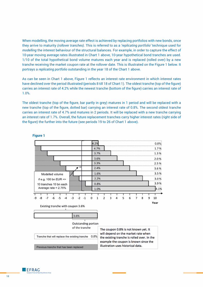
When modelling, the moving average rate effect is achieved by replacing portfolios with new bonds, once they arrive to maturity (rollover tranches). This is referred to as a ‘replicating portfolio’ technique used for modelling the interest behaviour of the structural balances. For example, in order to capture the effect of 10-year moving average rates illustrated in Chart 1 above, 10-year hypothetical bond tranches are used. 1/10 of the total hypothetical bond volume matures each year and is replaced (rolled over) by a new tranche receiving the market coupon rate at the rollover date. This is illustrated on the Figure 1 below. It portrays a replicating portfolio outstanding in the year 18 of the Chart 1 above.

As can be seen in Chart 1 above, Figure 1 reflects an interest rate environment in which interest rates have declined over the period illustrated (periods 8 till 18 of Chart 1). The oldest tranche (top of the figure) carries an interest rate of 4.2% while the newest tranche (bottom of the figure) carries an interest rate of 1.0%.

The oldest tranche (top of the figure, bar partly in grey) matures in 1 period and will be replaced with a new tranche (top of the figure, dotted bar) carrying an interest rate of 0.8%. The second oldest tranche carries an interest rate of 4.7% and matures in 2 periods. It will be replaced with a new tranche carrying an interest rate of 1.7%. Overall, the future replacement tranches carry higher interest rates (right side of the figure) the further into the future (see periods 19 to 26 of Chart 1 above).

Figure 1

19

The average rate for the current period becomes 2.75%. That percentage is derived from the average of each existing tranche in the current period. I.e. 4.2% + 4.7% + 3.7% + 3.6% + 3.3% +2.4% +1.6% +2.2% +0.8% +1.0%.

When modelling, banks use several rollover frequencies (daily, monthly, quarterly, yearly) but generally do not go beyond a one-year frequency. This influences the number of tranches needed to cover the total modelled volume. For example, if monthly rollover frequencies are used then 120 tranches are necessary to cover the total volume of the portfolio replicated on 10-year moving average basis (i.e. 12 tranches each year covering the 10-year period).

In practice, banks allocate all interest bearing items - both assets and liabilities - into time buckets in which they track any open interest rate risk position. When applying this technique to structural balances banks need to define at what moment in time – portion of – the structural balance falls due in order to close the interest position with the assets. That is, a portion of the structural balance is “locked” for a time period necessary to fund the corresponding assets. In order to determine the moment in time at which the portion of the structural balance falls due, behavioural estimates of deposits and/or the duration and interest profile of the assets are used.

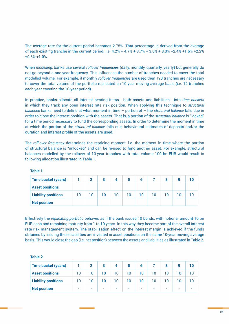
The roll-over frequency determines the repricing moment, i.e. the moment in time where the portion of structural balance is “unlocked” and can be re-used to fund another asset. For example, structural balances modelled by the rollover of 10-year tranches with total volume 100 bn EUR would result in following allocation illustrated in Table 1.

Effectively the replicating portfolio behaves as if the bank issued 10 bonds, with notional amount 10 bn EUR each and remaining maturity from 1 to 10 years. In this way they become part of the overall interest rate risk management system. The stabilisation effect on the interest margin is achieved if the funds obtained by issuing these liabilities are invested in asset positions on the same 10-year moving average basis. This would close the gap (i.e. net position) between the assets and liabilities as illustrated in Table 2.

Time bucket (years) 1 2 3 4 5 6 7 8 9 10

Asset positions

Liability positions 10 10 10 10 10 10 10 10 10 10

Net position

Table 1


Asset positions 10 10 10 10 10 10 10 10 10 10


Net position - - - - - - - - - -

Table 2

20

Table 3

Investing in assets on the basis of the replicating portfolio stabilises the interest margin. If the rates on structural balances were zero the interest margin would be exactly at the level of the moving average rates illustrated in the charts above.

If no modelling was used and contractual duration of deposits was used instead it would imply that all deposits are allocated to the shortest-term time bucket and thus treated as overnight deposits. This would require a bank, in order to fill the duration gap between assets and liabilities, to invest in assets on a very short-term basis. The net interest margin would be volatile (if the interest rates on structural balances were zero the volatility would correspond to the variability of short-term rates which can be seen on the Charts 1 and 2 above).

Thus, modelling of structural balances generally results in a stabilising effect. However, in recent banking history, situations have occurred when extremely high overnight interest rates were set by monetary authorities. In such exceptional cases, the use of longer duration assets issued at lower rates would lead to significant losses.

ACCOUNTING ASPECTS OF MODELLING STRUCTURAL BALANCES

If funds from structural balances are invested in assets that are measured at amortised cost, reported profit or loss includes interest income and interest expense. The accounting does not create any additional volatility in the interest margin.

In practice, however, there might be a mismatch between the expected maturity of banking book assets and liabilities. To achieve the desired matching, derivative contracts may be used for interest rate risk management purposes. For example, in case of a duration mismatch, the bank may need to swap variable interest rates for fixed interest rates by using interest rate swaps. The overall outcome would be a replicating portfolio where the fixed interest cash inflows are achieved as a synthetic effect of the variable interest rate assets and the swaps.

This is illustrated in Table 3 below in which funds from structural balances replicated by a 10-year roll-over portfolio are invested only in variable rate financial assets.6 As illustrated in Table 3 this results in all the assets being concentrated in the shortest time bucket while liability positions of modelled structural balances are spread evenly over all of the time buckets. The positions are not closed and the margin would not be stabilised.


Asset positions 100 - - - - - - - - -


Net position 90 10 10 10 10 10 10 10 10 10

6 The extreme case of a bank investing structural balances only in variable interest rates assets is used to provide a simpler explanation. In reality portfolios of banks are a mix of fixed and variable rate assets. Therefore, the need to use derivatives in order to build up a replicating portfolio would relate only to the volume in which in which structural balances are invested in variable interest rate assets. It has to be noted that, in interest rate risk management by banks, interest derivatives are not only used in connection with structural balances

21

The stabilisation effect is achieved using a portfolio of interest rate swaps which receive a fixed and pay variable interest rate. The variable cash flows from the swaps offset variable interest cash flows from the financial assets leading to overall fixed interest cash flows. Such a portfolio of interest rate swaps is also built up on the 10-year rollover basis. This closes the gaps in all the time buckets and the interest margin is stabilised. This is illustrated in Table 4.

One could argue that an accounting issue arises when a bank uses derivatives in its management of interest rate risk. Derivatives are measured by default at fair value through profit or loss, in contrast to most of the financial assets in the banking book. The overall effect is that profit or loss is volatile despite achieving stabilisation of the interest margin in terms of cash flows. However, this accounting mismatch is only one part of the problem. Banks do not hedge the interest income on the assets, rather the hedges are used to stabilise the net interest margin, thus taking into account the interest expenses from the liability side (i.e. structural balances). Current hedge accounting does not deal with structural balances in the way described as being used for risk management by an entity.

THE EXTENT OF THE STABILISATION EFFECT

For modelling purposes, structural balances are usually split into core and non-core parts.

Non-core structural balances are the portion that, based on the bank’s modelling, is subject to greater uncertainty and is not predicted to remain available over the modelling period. For example, the bank’s modelling might predict that the related portion of demand deposits will be withdrawn or equity reduced by future losses.

Core structural balances are the portion that, based on the bank’s modelling, is stable and predicted to remain available over the modelling period. In the case of demand deposits, the core part is that which is not expected to be withdrawn and is not subject to changes in interest rates during the modelled period. In the case of equity (which is not interest sensitive), the core part is the total less the volatile volume captured by the non-core part.

Table 4


Asset positions 10 10 10 10 10 10 10 10 10 10


Net position - - - - - - - - - -

22

Figure 2

The replicating portfolio relates to the core part7 of the structural balances. As can be seen in Figure 2, the maturities of the roll-over tranches form a triangle within which balances are expected to be reasonably stable in terms of:

a) clients; and

b) the client rate does not change8.

This is illustrated in Figure 2:

Abbreviations used in the above figure

CDD: Core Demand Deposits

The extent of stabilisation should be understood as the difference between the modelled moving average rate and the short term rate. Charts 1 and 2 above provide an example of the extent of the reduced volatility: this can be seen by comparing the movement in the long-term moving average with short-term interest rates.

7 If certain stability is identified for the non-core part banks may build separate shorter-term, e.g. up to 2 years, replicating portfolios also for this part.8 The client rate of some types of savings or similar accounts may change to reflect the movements in the market rate. But this does not happen in a way

fully correlated with specific money market rate (which should be used for modelling if this was the case). For example, the client rate movements may correlate with moving averages of shorter-term rates (e.g. 2 years) in which case they are considered stable within the horizon of the 2-year moving average replicating portfolio triangle

23

Often the balances may not reprice and not mature even beyond the period modelled in the replicating portfolio. This is typical of the core part of equity. For demand deposits, the expected duration is increased, if the bank takes into consideration replacements of the withdrawn balances by new money deposited in the same product. From this perspective, certain balances may be extremely long-term (even perpetual).

To the extent that the structural balances are expected to be stable beyond the modelled time horizon the overall interest margin of the bank retains some volatility. This is displayed on Chart 3 below which uses an extreme case of structural balances that are expected to remain into perpetuity. In such a scenario the fund from these structural balances that could, in theory, be invested in perpetual rate-assets (which are assumed to have an interest rate of 3.0% in the chart). This strategy would fully stabilise the interest margin. However, the structural balances are modelled and invested on 10-year moving average basis.

Chart 3 uses data from Chart 1. It focuses on the differences between the theoretical perpetual interest rate of 3.0% and the rate that would be achieved under alternative strategies. The line labelled ‘Short-term rate volatility removed’ illustrates how much of the short-term rates volatility would be removed if structural balances were invested in 3% rate perpetual assets. The line ‘Residual 10-year MA rate volatility retained’ shows the residual volatility if the funds from structural balances are invested on a 10-year moving average basis rather than in perpetual rate assets.

Chart 3

24

Investing based on an objective of achieving the long-term moving average rate stabilises the interest rate margin significantly compared to investing on a short-term basis, but the margin still retains some volatility. However, this residual volatility is not considered as risk for interest rate risk management purposes.9

Modelling practices applied by banks differ. If the actual behaviour differs from the modelling of the structural balances, the stabilisation effect is only partially achieved (i.e. the period over which the maturity is modelled is shorter or longer than the actual period over which the structural balances behave as a fixed rate funding source).

As risk management is a dynamic process, the differences resulting from actual behaviour compared to expected behaviour, will be addressed through adjusting the interest rate position of the entity.

VIEWS FROM REGULATORS

Banking supervision authorities ask banks to apply caution in their stabilisation strategies for demand deposits and equity.

The European Banking Authority (EBA)10 refers to opportunity costs arising from stabilising the margin by stating: “Clearly, the downside of locking in a margin under a scenario of falling rates is that the institution will be less able to benefit from the additional margin potentially available under a rising rates scenario.” Similarly, in respect of equity EBA says: “In deciding the investment term assumptions for equity capital, institutions should avoid taking income stabilisation positions that significantly reduce their capability to adjust to significant changes in the underlying economic and business environment.” EBA also refers to a possibility of earlier than expected repricing of the liabilities: “Therefore, although an institution may be able to demonstrate to itself that the balances will remain (at substantially unchanged rates) for a very long period, it will nonetheless wish to ensure that the benefits of locking in returns to match the expected repricing profile outweigh the risks that the balances may decay/reprice more quickly than anticipated, potentially resulting in the locked-in return on assets being less than the repriced cost of funding them.”

9 For the treasury unit of the bank which is in charge of interest rate risk management, the risk exists up to the modelled time horizon (10-year in the example) but not beyond it. From this perspective the interest risk position would be closed (if structural balances were invested in assets with the same moving average rate interest rate profile – 10-year rollover investment strategy in the example). However, the total interest income of the bank would be subject to the residual volatility resulting from changes in the moving average rates (10-year moving average assets vs. fixed rate on the liability/equity in the example). This volatility would stay with the business units of the bank (e.g. a branch collecting the deposits) rather than with the treasury unit.

An internal fund transfer pricing mechanism is used for this purposes. The business unit sells the funds received from a demand deposit, via an internal loan, to the treasury unit. The business unit records interest income e.g. on a 10-year moving average basis resulting from the internal loan. Compared to zero interest rate paid on the demand deposit this would result in the interest margin of the business unit moving in correlation with the 10-year moving average rate.

10 Guidelines on the management of interest rate risk arising from non-trading activities issued by EBA on 22 May 2015

25

In addition, EBA points out that the stabilisation may result in risk calculated on an economic value-basis: “…the key issues are the prudence of the assumptions made, and whether an appropriate balance is being struck between earnings stabilisation and economic value risk arising.”11 The Basel Committee12 also points to the resulting compromise between the stabilisation and economic value risk in respect of non-maturity deposits by stating: “The maturity profile chosen will therefore be a compromise between protection of earnings for an extended period and increased risk to economic value that could materialise on a shock event (e.g. a deposit run on non-maturity deposits, failure of the bank).” while for equity it says: “…banks determine their own strategies for managing the earnings volatility that arises from it using techniques similar to those for non-maturity deposits.”

11 Economic value metrics are a present value-based measure. The result highly depends on how maturity of structural balances is treated. ‘Economic value of equity’ indicator does not ascribe maturity to equity (i.e. equity is not modelled as also required for the standardised regulatory calculations). Therefore, the risk arises when equity funds longer-term assets despite the stabilisation effect of such strategy on the net interest income. The economic value risk would be further enhanced if demand deposits funding longer-term assets were not included in the measure on modelled basis. However, if the economic value metrics reflected structural balances on modelled basis (both equity and demand deposits, as applied by some banks in their internal economic-value-based metrics) this would significantly reduce if not remove the contradictions between the earnings- and economic value-based metrics.

12 Standards: Interest rate risk in the banking book issued by Basel Committee on Banking Supervision in April 2016.

26

FINDINGS FROMTHE OUTREACH

PURPOSE AND NATURE OF RISK MANAGEMENT ACTIVITIES

PARTICIPATING BANKS

Fifteen banks participated in the outreach, of which fourteen were commercial banks. One bank was involved in specialised activities. The banks came from different jurisdictions within Europe (within the euro-zone and beyond). All except one of the banks participating in the outreach invested mainly in fixed interest rates assets. For confidentiality reasons the names of the participating banks are not published.

Except one bank not collecting deposits, banks held a weighted average of 43,5% of client deposits on their balance sheet, however this weighted average represented a range between 67% and 28% of client deposits being held.

PURPOSE OF THE RISK MANAGEMENT ACTIVITIES

The purpose of interest rate risk management was generally described as stabilising net interest income. However, some of the banks have indicated that once the net interest income has been stabilised and once all the regulatory requirements have been fulfilled, “optimisation” of the net interest margin could occur.

Optimisation was generally understood as leaving interest rate risk positions “open”. One bank indicated that the optimisation of net interest income was done on the product level (business pricing, product volumes, business strategy, etc.) and that it was not done within the interest rate risk management.

All banks indicated that the purpose of their risk management activities remained the same over time and did not depend on the overall structure of the balance sheet.

All of the banks had asset and liability management (ALM) and asset and liability committees (ALCO) at group level where the main decisions were taken. All the banks had internal processes and policies that defined how and when to perform the monitoring of the net interest margin.

Balance sheet total 15 banks in millions EUR

Client deposits 14 banks in million EUR

Weighted average of client deposits 14 banks

15.161.174 6.369.864 43.5%

27

INDICATORS USED TO MONITOR THE INTEREST RISK

Banks used and combined a wide range of quantitative and qualitative tools to evaluate the extent of success/failure of their interest rate risk management activities and strategies. Quantitative limits were used for sensitivities, value at risk, stress tests, scenario analyses and ratios on economic capital. The main indicators used by the banks to monitor the net interest margin were the following:

a) Value-based indicators

(i) Economic Value of Equity13; (ii) Value at Risk14; and(iii) Present value of interest rate gaps15.

b) Earnings indicators

(i) Annual earnings at risk16; or similarly(ii) Sensitivity of the net interest margin17.

Most of the banks usually made risk management decisions based on the net interest rate risk arising from a combination of financial assets and financial liabilities. They often used a sensitivity analysis with a maturity (duration) time band approach.

STRUCTURAL BALANCES MANAGEMENTThe overarching objective of modelling structural balances for the banks participating in the outreach was to stabilise net interest income.

All the banks integrated their interest rate risk management of structural balances into their overall interest rate risk management in the banking book. If banks applied optimisation strategies of net interest income this was applied at the level of the total banking book rather than with a specific a focus on structural balances.

Two banks provided additional background on specific aspects of their structural balances management.

One bank allocated the structural balances (core part of demand deposits and equity) in a separate book which was part of the banking book. This separate book for structural balances was invested in long-term maturity assets and the rest was transferred to the other part of the banking book through long-term internal funding. However, even when the banking book consisted of separate books the overall position was managed.

13 Economic Value of Equity is a cash-flow calculation comparing the present value of expected cash flows of liabilities and assets.14 Value at Risk measures the potential loss in value of generally a portfolio of financial assets over a defined period for a given confidence interval.15 An interest rate gap report assigns interest cash flows of both assets and liabilities to the time buckets at which they are expected to occur, allowing to calculate the present value of the (net) interest cash flows and thus the exposure of the bank to interest rate risk. 16 Annual earnings at risk measures the sensitivity of net interest income for a one-year period. It is calculated as the difference between the estimated income using the current yield curve and the lowest estimated income following an increase or decrease in interest rates of x basis points.17 Interest rate sensitivity measures how much the net interest margin will fluctuate as a result of change in the market interest rate environment.

28

Another bank explained that it used a risk tolerance range (e.g. +/- 1 year) around the modelled maturity of structural balances when determining the possible investment range of these balances. The asset and liability committee decided about the current target maturity for investments within this range.

Items constituting structural balances were predominantly demand deposits and equity (including non-financial items by some banks). Their modelling as described by the banks is discussed below.

In addition, one bank mentioned that structural balances could arise from administrated rate products for the part of the contractual rate which does not track market rates. Another source could be term deposits with a notice period because, unless the notice has not been exercised, the maturity could not be defined. For another bank structural risk arose also from its credit cards portfolio where the balances are regularly fully repaid and thus no interest was charged. They effectively behaved as revolving non-interest bearing assets.

MODELLING CORE DEMAND DEPOSITS

INTRODUCTION

All but one of the banks that model demand deposits distinguished between:

a) the core part; and

b) the non-core.

However, one bank modelled all demand deposits as one homogenous group. Another bank did not use such a bright line split for larger customers which were modelled as one group. For other customers the split was applied.

One bank provided the following three-level internal categorisation of demand deposits in order to identify the core part:

a) non-maturing deposits – i.e. repayable on demand;

b) staying with the bank for the foreseeable future; and

c) not priced to reference rate or index (i.e. index such as central bank rate).

These features were aimed at identifying the part of demand deposits which will be available to the bank for the longer-term during which the contractual rate does not change or the change is uncorrelated to market rates. As a result, the core demand deposits were considered as a fixed rate liability over the term during which the contractual rate does not change or the change is uncorrelated to market rates. This categorisation was not explicitly mentioned by other banks but the three of the features could be observed in their modelling practices.

29

One bank also mentioned, that in order to be available for modelling, the product should also be individually priced.

FACTORS FOR CORE / NON-CORE PART DETERMINATION

The models used by the participating banks were based on long-term historical time series showing the level of volatilities and seasonality of the volumes. The banks used several factors to determine the core and non-core parts. They are stated in the order of frequency mentioned by banks:

a) product and client type was used by all except one of the banks. In this respect balances on retail current accounts were generally more stable than on savings accounts and on current accounts of small and medium-sized entities, municipalities and corporates. One bank no longer considered product as the determining factor and focused on customer type;

b) country;

c) usage for transactional purposes, e.g. payment accounts tend to be more stable;

d) sensitivity of the volume of deposits to levels of market interest rates - accounts which do not react to (i.e. are not withdrawn due to) changes in the market interest rates tend to be more stable. Sensitive accounts are those that may be withdrawn when interest rates increase. These deposit accounts may be excluded from the core part or modelled with a shorter duration;

e) deposit accounts with smaller amounts tend to be more stable (i.e. have higher core part) than deposit accounts with high amounts;

f) numbers of products held by a customer balances with customers holding multiple products tend to be more stable; and

g) political factors.

Some of these factors are interrelated, e.g. whether the account is transactional depends to a large extent on the product type. Savings accounts are generally less suitable for transactional purposes. Further, savings account products tend to be more sensitive to the market interest rates (i.e. are more likely to be withdrawn when interest rate increase) compared to current accounts used for transactional purposes.

30

The one bank which did not distinguish between the core and non-core part of demand deposits was focused only on the product type. This bank treated each product differently for modelling purposes, depending on its client interest rate characteristics.

Banks generally observed that, in the current low interest rate environment, demand deposits have been increasing in overall volume but the increase is mainly in the non-core part. In this respect one bank specifically noted that those accounts which paid no interest but would pay if interest rates increased were excluded from the core part and assessed separately with a dedicated replicating portfolio. Another bank stated that the increase in balances after the global financial crisis in 2008 was considered as unstable and largely unavailable for modelling purposes.

One bank did not identify sensitivity of the core/non-core part to the current low rates environment which was due to the fact that they focused on demand deposits balances at the client rather than product level. They observed a substitution between fixed rate (such as current accounts) and variable rates demand deposit accounts. In the low interest rate environment, balances tended to move into variable rate accounts but remained stable at overall client level. This behavioural trend was confirmed by another bank at which the level of interest rates was a driver only for changes in volumes of particular products used by a client. One bank did not record migration to the non-core part of demand deposits in the current low rates environment.

One bank noted that for new products, the lack of historical trend data and related uncertainty about future behaviour would be considered in the modelling.

Models used by the banks were generally dynamic, i.e. the proportion of core and non-core part could change based on evolution of the applicable factors. One bank referred to its model as a model not based on probability factors, i.e. which was not sensitive to interest rates and the core volume was determined in absolute terms requiring a management decision to change the core deposit amount.

NON-CORE PART MATURITY

The participating banks took different approaches to assigning what maturities to the non-core part of their demand deposits. Seven banks were specific in this respect.

Three banks treated the non-core part as having overnight maturity. This is despite the fact, as noted by one bank, these balances were exposed to changes in interest rate. Two banks assigned one-month maturity to their non-core demand deposits, while one of these banks also a distinguished a seasonal part for current accounts which was modelled with a three-month maturity.

Two banks modelled the maturity of the non-core part on product-by-product basis, starting with overnight maturity up-to longer maturities if the balances were considered to be available over this horizon (e.g. 2 years). For one of these banks balances which were available for a longer period but were not stable enough to be considered core deposits, were treated as a separate layer and modelled over a short term horizon. For example, balances collected due to low rates environment fell under this treatment.

31

CORE DEMAND DEPOSITS VOLUMES

Most of the banks analysed the volumes of core demand deposits in respect of existing balances, i.e. they did not consider future growth. One bank considered growth over a 3-year period (in line with forecasting/budgeting horizon which was reflected in the net interest income sensitivity indicator used for risk management purposes).

Once the volume had been determined banks considered withdrawals/outflows of the balances, i.e. the liquidity factor. Banks differed in respect of whether and how they consider replacement of withdrawn balances by new deposits (also referred to as replenishment of new balances, drawdowns and fill-ups).

Eight banks took such replacements into consideration. One of these banks noted they also modelled how long it took on average by existing customers to withdraw balances and this was one of the factors when determining duration of the core part. The reason for this being that hedging (stabilisation of net interest income) after the time the customer was expected to leave the bank may be problematic. Another bank which used the static approach mentioned that from a replacement perspective the balances were perpetual as they had never recorded a decrease in the core part. However, they did not consider that perpetual horizon in the actual maturity modelling.

Three banks focussed only on run-off/outflow of balances of existing customers, i.e. how much of these balances that were expected to remain after specific time period.

One bank used a combination of these approaches. It considered new production over a 3-year period (in line with the 3-year period over which they also considered growth of balances) and run-off of those balances thereafter.

One bank applied a cap (of up to 90%) to the proportion of its non-volatile deposits that is modelled. The reason for excluding the 10% portion is to take account of seasonality and risk of migration to different products. Management might vary the percentage in order to capture higher migration risk in a very low interest rate environment.

CORE DEMAND DEPOSITS MODELLED MATURITIES

Banks determine the maturity of demand deposits used for interest rate risk purposes (i.e. about the modelled maturity, such as determining the length and number of bond tranches in the replicating portfolio). The volume of the core demand deposits and time horizon of their availability (on an un-repriced basis) put limits on what maturities banks could assign to the deposits.

For banks which took into consideration new production of core demand deposits (which extended the availability horizon theoretically into perpetuity) the modelled maturity could be significantly shorter than the expected one. In this respect one bank noted that for example for private customers, core demand deposits were very stable and therefore the outflow (liquidity) profile was not a limiting factor in assigning the maturity. However, this might not be true for corporate customers.

32

Banks which considered replacements of existing core demand deposits by balances coming from new customers generally referred to the final maturity being determined based on a management decision. They mentioned following drivers:

a) appetite for income volatility;

b) asset-driven management decision;

c) stabilisation of net interest income over interest cycle;

d) own risk management strategy and bank’s risk appetite; or

e) trade-off between stabilisation and a risk that balances may migrate to different products over a long-term horizon which was subject to several additional constraints which are detailed below.

One bank did not distinguish between the core and non-core part. The modelled maturity was a combination of contractual client interest rate behaviour and expected withdrawals given the market rates environment.

For three banks which focussed on withdrawals of balances from existing customers it was the run-off / outflow profile statistics which determined the maturity.

Regarding the asset-driven management decision referred to above, two banks assigned the maturities with the aim of achieving a natural offset against the assets without using derivatives. For example, if a large volume of mortgage loans with a 10-year fixed rate was available to cover the core demand deposit balances, a 10-year maturity would be assigned to those balances. One of these banks noted that a longer time horizon was more effective stabilising the net interest income. For another bank the availability of assets to achieve natural offsets was an important consideration but, this bank also considered other factors such as the unfavourability of investing over the long term in the current low interest rate environment.

Certain elements of the asset-driven (or derivative-driven) decision were mentioned by two other banks. For one of these banks, a possibility of achieving natural offset with assets was a factor that might restrict them in some markets when assigning a maturity which might be well below the modelled run-off profile. For example, if in a specific market, no long-term swaps existed and most of the loans had short-term interest rates, the bank would limit the modelled maturity to 2-years as a result of these market conditions. Similarly, another bank mentioned that the existence of liquid interest rate swaps with respective maturities might be a limiting factor in some less developed markets.

33

One bank considered several factors in the management decision about the tenor of the modelled rates as mentioned above. Some of the modelled rates can be understood as asset-driven. These were focused on finding capacities to accommodate the modelled maturity:

a) market capacity to achieve a hedge through natural offset with assets or through derivatives. E.g. in some market there may be no fixed rates assets or derivatives, or a liquid market may not exist at all.

b) amortised cost accounting in order to achieve a natural hedge without fair value accounting. Use of the held-to-maturity portfolio in IAS 39 did not provide a solution because of the taint-ing rule, i.e. the restriction that financial assets in this portfolio had to be held until maturity. The classification of financial assets under the held to collect business model in IFRS 9 not applying tainting rules would improve this situation.

c) capacity to classify the assets as available-for-sale (AFS) if there is not derivative market, revaluation of AFS assets through other comprehensive income causes volatility in regulatory capital; and

d) credit risk from a risk-weighted assets perspective when investing in sovereign bonds.

Five banks noted that their decision to stabilise net interest income was not linked at all to maturities of assets (or derivatives).

Some banks were specific in mentioning the actual ranges of assigned maturities. One bank mentioned maturities between 10 and 15 years, another bank between 3 and 6 years. One bank specified 10-year maturity in respect of their zero rate demand deposits. Another bank applied 10-year cap to maturities on non-interest bearing demand deposits which could be further reduced by a set of capacity constraints discussed above.

Two banks provided the information in relation to their replicating portfolios whose maturities ranged from 1 to 15 years and for the other bank from 1 month to 10 years (in order to capture different interest stability of demand deposits ranging from money market-linked products to corporates to zero rate current accounts).

More information was provided by banks in respect of frequency of the rollover tranches on the replicating portfolios. Monthly tranches were used by eight banks, with one of these banks using also quarterly tranches in some cases. One bank used yearly tranches and one bank daily tranches.

34

Modelled maturity of demand deposits is addressed by regulators which impose limits in this respect18. Banks generally considered them in their modelling. One bank specifically stated that there would be no point in running two different models for regulatory and internal purposes. But they also stated that the existing requirements did not restrict them in assigning the maturities.

CONSIDERATION OF CONTRACTUAL RATES OF DEMAND DEPOSITS

Core demand deposits are generally considered to be of a fixed-rate nature. The volume or demand deposits which is stable from outflow perspective would not be available as core volume if the contractual rate changes (i.e. they re-price) in correlation with market rates. Put in other words, demand deposits are not available as core beyond their re-pricing time horizon.

All the banks that modelled core demand deposits used the premise that they had a contractual interest of a fixed-rate nature, i.e. the variable rate part was excluded. In that respect they mentioned the following:

a) Products were split into a part which tracked the market rate and the core part which did not. The banks also noted that interest rates on demand deposits were generally close to zero. One of the banks said that their model was based on the premise that the accounts did not pay a contractual rate or the rate changed very slowly. There had been a product in its portfolio which tracked money market rates and had been subject to a separate treatment but was no longer offered;

b) The large majority of core demand deposits behaved as fixed rate, i.e. the interest rate attributed to these demand deposits did not change even when market interest rates changed and the remaining volatility of the contractual rate was not a concern;

c) If products had a changing interest rate, the interest rate behaviour was modelled and the products were treated as partly fixed and partly variable;

d) Deposit rate elasticity was considered – for example if 60% of market rate movement was passed to customers then 40% behaved as non-interest bearing deposits and was available for modelling on a long-term basis. One bank applied this approach specifically to demand deposits with managed (i.e. administrated) rates and the passed rate (60%) was modelled on a very short-term basis with 1-month or 3-month, exceptionally 6-month tenors;

e) Core demand deposits contractual rates were generally very stable and often zero for current accounts. If contractual rates were correlated with market rates for certain demand deposits, those deposits would not be considered as core for the full maturity profile but would instead be allocated into time buckets according to the modelled repricing profile; and

18 Guidelines on the management of interest rate risk arising from non-trading activities issued by EBA on 22 May 2015 require that the assumed behavioural repricing date for customer balances (liabilities) without specific repricing dates should be constrained to a maximum average of 5 years (computed as the average of the assumed repricing dates of different accounts including both stable and the volatile portion). This requirement is relevant for calculation of economic value of equity indicator that result from calculating the outcome of the standard shock, as referred to in Article 98(5) of Directive 2013/36/EU (sudden and unexpected change in interest rates of 200 basis points).

Standards: Interest rate risk in the banking book issued by Basel Committee on Banking Supervision in April 2016 require that banks disclose, for reporting to a competent authority, the measured change in economic value of equity under prescribed interest shock scenarios. In this respect supervisors could mandate the banks, or the banks may adopt, a standardised framework. In respect of non-maturity deposits, the standardised approach distinguishes between retail/transactional accounts, retail/non-transactional and wholesale deposits and imposes caps on proportion of core deposits 90%, 70% and 50% respectively and caps on average maturity of core deposits 5, 4.5 and 4 years respectively. In addition to the required disclosures banks are encouraged to make voluntary disclosures on internal measures of interest rate risk in the banking book.

35

f) Core volume was related only to non-interest bearing deposits. If contractual rate changed but in a way not clearly linked to market reference rate, the interest rate behaviour was modelled. The bank applying this approach treated the fixed rate demand deposits separately from the demand deposits with an interest rate correlated to market rates. This bank also stated that changes in the contractual rate beyond the modelled interest rate component did not belong to interest rate risk in the banking book but were considered as commercial or margin com-pression risk which was a business risk.

One bank applied an approach based on modelling of different future interest market rate scenarios for interest sensitive demand deposits. The model determined what would be the expected contractual interest rate in each scenario. This reflected past behaviour and current pricing strategies. The expected repricing profile was the outcome of such modelling.

Similarly, another bank determined the distribution of expected client interest rates paths. For each product they built a replicating portfolio that best fit the rates behaviour (using the mean of those paths, the best fit to achieve a stable product margin). The outcome might be a basket rate such as 50% 3-month rate + 50% 5-year rate (rates from 1 month to 10 years were available in that respect). Another bank used a similar approach (best fit, constant margin) for the core part of their savings demand deposits based on historical analysis of client rates behaviour considering also withdrawals of the balances. It resulted in a basket rate maturity assigned to the deposits combining a short and long-term rate.

Banks not modelling demand deposits

Two banks did not model demand deposits. One of them was a specialised bank whose business model did not involve collecting demand deposits.

The other bank used demand deposits to fund its short term lending or liquidity reserves in central banks. There were two main reasons for that:

a) It created liquidity risk to use deposit contracts to finance long-term funding; and

b) The local supervisor considered all deposit contracts to be overnight funding when calculating capital requirements for the interest rate risk in the banking book.

The latter reason implied that any maturity mismatch (according to the regulatory approach) would give rise to an extra capital requirement. The bank acknowledged that demand deposits could be used as a funding source for shorter durations based on prudent modelling. However, the extra return created by using demand deposits instead of wholesale funding, did not generate sufficient returns to compensate for the extra capital requirements. At the margin, the bank modelled some demand deposits, other than transaction accounts, and used them as funding for lending exposures with 3-month duration and interest rate fixing.

36

INTERACTIONS BETWEEN LIQUIDITY RISK AND INTEREST RATE RISK MANAGEMENT

Generally, banks leveraged their liquidity risk management systems focused on outflows of funds in order to obtain the data relevant for interest risk modelling of demand deposits. In this respect banks stated:

a) There was an interaction with liquidity risk in a way that higher risk of outflow would result in shorter-term maturities;

b) The models used for liquidity risk purposes were similar but not identical. For example, 3-month term deposits might have a long-term maturity in the liquidity model, but not for interest rate risk purposes. Core volume may also differ;

c) Modelling for liquidity (outflow profile) risk was also the main input for interest rate risk management (two banks). One of these banks stated that for zero rate demand deposits the modelled maturity for liquidity risk purposes was the same as used for interest rate risk management;

d) Interest rate modelling takes into account liquidity modelling; and

e) Analysis carried out for liquidity coverage purposes was leveraged for the interest rate risk management purposes (such as breakdown into transactional and non-transactional accounts, analysis of stable balances). However, banks also noted that liquidity risk was asymmetrical (risk results from earlier outflows than expected). On the other hand, management of interest rate risk in the banking book took a symmetrical perspective (risk arises from both shorter and longer interest rate exposures), considered contractual interest rate behaviour and was based on a going concern framework.

Four banks referred to their liquidity risk modelling as being separate. However, one of these banks also noted that the models can be partly the same. The differences arose for example for savings accounts which had partly a variable rate. Another bank stated that the liquidity view was part of the behavioural analysis of customers and from that perspective there was an interaction with the interest risk modelling.

37

MODELLING EQUITY

INTRODUCTION

Eight of the participating banks modelled the maturity of equity.

Three banks considered non-financial items in defining maturity of equity, i.e. they considered that equity was partly invested in non-interest bearing assets which were expected to have the same maturity as equity (for example real estate, equity investments or intangible assets). By doing so, shareholders were assigned a long-term economic income from their investment. Two of those banks also integrated liabilities in their definition of equity such as loan loss provisions and tax liabilities. Many of these items were expected to have the same maturity as equity. For other non-financial items (e.g. tax liabilities, litigation provisions) the expected settlement horizon was taken into account in their modelling. One bank included those non-financial items which had historical funding aspect mentioning goodwill as the main example, excluding sundry assets and liabilities which resulted from accrual accounting.

One of these three banks further divided the non-financial items and equity into stable core part whose maturity was modelled and non-core part which was put into overnight time bucket. The amount of the modelled equity was increased in relation to earned profits but this always required a management decision. Their amount of equity was based more on national GAAP than IFRS, where the main difference was in respect of revaluation items in OCI due to which such equity had more ‘paid-in’ or ‘cash’ character. Another bank considered the volatility part through the 90% cap applied on the modelled part (the same approach as they applied for demand deposits).

Three banks modelled accounting equity net of non-interest bearing items, i.e. such equity was the difference between interest-bearing assets and interest-bearing liabilities. Two of them further noted that in modelling, they excluded the liquid part which would not be available for a long time. One of them specified that the liquid part included items such as dividends and taxes to which maturities were assigned based on the expected pay-out horizon. One bank netted the equity against goodwill and property assets. A targeted duration was specified for investments of such an equity and the actual duration could deviate within limits in which staff in charge of investing the equity could operate. Average duration was two to five years depending on currency.

One bank noted that the amount of modelled equity was similar to IFRS accounting equity and they also considered future equity inflows and outflows in respect of acquisition activities but not for future earnings or dividends.

For another bank the amount of modelled equity was driven by IFRS accounting equity but this bank did not model the full amount. They also specified the modelled maturity term as being 10 years by using rollover tranches on quarterly basis.

Other banks modelling equity confirmed that they used replicating portfolio based on rollover tranches. Six of them specified that they used monthly tranches in this respect with one of them using also quarterly tranches in some cases.

38

The dominant factor for assigning the maturities to the modelled equity was a management decision with the main objective being to stabilise net interest income volatility. The banks which specified their basis for this decision stated:

a) The main objective was to smooth net interest income volatility;

b) Maturity was in line with risk appetite with the aim of through-the-cycle stabilisation of net interest income;

c) Long-term horizon over which they want to stabilise net interest income; and

d) Trade-off between stabilising the net interest income and locking in the margin for too long would result in over-stabilising.

Generally, it was not observed that the management decision about modelled maturity of equity was driven by the maturity of existing assets in order to achieve a natural offset. Two banks explicitly confirmed this. However, one bank noted that the assigned maturity could also be explained by the existence of long-term fixed rate loans in order to achieve a natural hedge.

All the banks that modelled equity confirmed that the approach used was generally very consistent overtime and that changes to the approach were rare.

Three banks confirmed that hybrid capital instruments classified as equity with debt-like cash flows (such as cumulative preference shares, instruments with discretionary fixed coupon and, hybrid Tier 1 capital instruments) would be treated as liabilities. However, one bank noted that the accounting classification as equity mattered. From the perspective of profit or loss volatility, the fixed nature of dividends was irrelevant since they were treated as distributions of earnings and instruments such as perpetual preference shares were included in the modelled equity.

BANKS WITH IMPLICIT MODELLING OF THE MATURITY OF EQUITY

Three banks modelled equity implicitly. In other words, they treated equity as being available for funding the duration of the assets it was invested in. However, they did not include such implicitly modelled maturity in computation of their risk metrics which was in line with regulatory requirements19 and kept the resulting open position within the required regulatory limits.

19 Guidelines on the management of interest rate risk arising from non-trading activities issued by EBA on 22 May 2015 require that equity capital should be excluded from liabilities, i.e. that it should not be modelled. This requirement is relevant for calculation of economic value of equity indicator that results from calculating the outcome of the standard shock, as referred to in Article 98(5) of Directive 2013/36/EU (sudden and unexpected change in interest rates of 200 basis points).

Standards: Interest rate risk in the banking book issued by Basel Committee on Banking Supervision in April 2016 require that banks disclose, for reporting to a competent authority, the measured change in economic value of equity under prescribed interest shock scenarios. In this respect banks should exclude their own equity from the computation of the exposure levels. In addition to the required disclosures banks are encouraged to make voluntary disclosures on internal measures of interest rate risk in the banking book (i.e. here the equity can be modelled).

39

In this respect, one of these three banks further specified that the duration of equity was not modelled since it considered equity to be perpetual. Instead equity was implicitly considered by treating the cost of equity as an interest expense in calculating the net interest margin of interest-bearing assets which were being funded with equity. However, the fact that equity was a long-term funding source was recognised in their mortgage subsidiary where equity was used for financing loans with a 3-year fixed rate. The allocation of equity to 3-year lending was done within the risk limits of the bank. The internal risk limits considered that the 3-year lending financed by equity was an open position. The same applied for the regulatory treatment; i.e. the regulator also considered the position to be an open interest rate position.

Another bank used a separate book for capital and its investments over a longer-term horizon. Average maturity of these investments was between 3 and 4 years.

BANKS WHICH DID NOT MODEL THE MATURITY OF EQUITY

Two banks did not model equity including other non-financial items for interest rate risk management purposes. One of these banks specified that this decision was based on regulatory requirements.

One bank did not model equity but included non-financial assets and non-financial liabilities in their interest rate risk management. The maturities were assigned based on assumptions used for internal performance management.

NET INTEREST MARGIN BROKEN DOWN BY PROFIT SOURCE

BREAKDOWN OF NET INTEREST MARGIN

Most participating banks had internal information about the different components of the net interest margin; which they used for management purposes. The granularity of the components differed between banks:

a) Some banks knew their commercial margins at individual loan level and/or for their current accounts and at a higher level of aggregation such as per business line, per product line, per geographical area, per individual bank in the group, or per profit centre;

b) One bank indicated they tracked separately the hedging result of interest rate risk;

c) Some tracked their asset and liability management result or treasury result separately. Of those that did, one bank indicated to have information available on the open position per underlying risk factor such as currency basis risk, credit risk or interest rate risk; and

d) Some banks had information available about the net interest income derived from structural balances, some did not.

40

Some banks did not have a breakdown of the net interest income available at consolidated level. Reasons provided for this were:

a) It was not considered in the asset and liability management, which had only one purpose of stabilising the net interest income; and

b) A detailed split was not considered to be useful information. Those banks used a breakdown at more aggregated level.

MATURITY TRANSFORMATION

In simple terms, banks have a maturity transformation function, i.e. they collect on average short-term liabilities and lend the money out to the economy to – on average – longer term assets. In doing so they earn a premium for the risk taken. In theory, the net interest margin is thus composed of three elements:

a) The margin earned on assets;

b) The margin earned on liabilities; and

c) The transformation margin.

However, in the outreach the transformation margin was described differently by different banks:

a) Earnings made when in particular time buckets the amount of interest bearing assets is higher than the amount of interest bearing liabilities, the interest income from the surplus of interest bearing assets is considered as the transformation margin; or

b) The product of the open position (unhedged interest rate risk position) times the movement in relevant market parameters (such as the market interest rate at that moment). As both factors were unknown at the beginning of the period, the transformation result was not forecastable.

Commercial sensitivity of the breakdown

Some banks were not in favour of disclosing components of the net interest margin as these were considered to be commercially sensitive. Some of these banks also noted that disclosing these data would provide competitors with insight into (i) how products are structured and (ii) under which interest rate scenario the bank is vulnerable given its products and the swap positions it has entered into to cover the interest rate risk related to those products. Hence competitors would be in a position to build a strategy creating products to outcompete the bank in the worst possible interest rate market environment.

41

Need for clear definitions

Transformation: Banks cautioned against providing comparability based on certain terminology as some of these terms were used differently by different banks. For example, some banks had a different interpretation on what ‘transformation’ meant. It was questioned whether assigning non-maturing liabilities to interest-bearing financial assets could be considered as transformation, or whether it was something else.

Optimisation: Also it was not clear whether or not transformation equalled optimisation (in contrast to stabilisation). If part of the core demand deposits was assigned to the interest-bearing financial assets would this be considered as optimisation?

42

Modelling of structural balances for interest rate risk management purposes is an established business practice within the banking industry. From a risk management perspective, modelling in the banking book is generally carried out in order to manage net interest income. Such managing consists of two components, a stabilisation component and an optimisation component. The use of the words ‘stabilisation’ and ‘optimisation’ are understood differently between risk management practitioners and accounting practitioners.

A more neutral way to describe the business practice of banks could start from the definition of interest rate risk. One could say that banks estimate the size of expected – contractual and allocated – interest cash flows and the future moment in time at which these are expected to occur. When portions of structural balances are expected to stay on the balance sheet for a defined period, a rate is allocated to that portion which can be an average rate and/or a rate that corresponds to the duration of the portion. Those estimations are continuously monitored and re-assessed in a dynamic process.

The reason for modelling of structural balances relates their interaction with the bank’s assets. Modelled longer-term maturity of structural balances enables the bank to invest in long-term fixed-rate assets which stabilises interest margin. Without modelling, structural balances would be treated as having zero maturity. This would encourage banks to invest in very short-term assets whose rates are generally very volatile and would reduce the finance available for longer term assets. As identified in the outreach, banks apply different modelling practices. Generally, they distinguish between a stable (“core”) part which is modelled on a longer-term basis and a more volatile (“non-core”) part. When modelling the period over which core demand deposits will remain available, some banks consider that withdrawn balances are replaced by new deposits. These banks tend to assign the maturity to demand deposits based on management assumptions about the future. Other banks focus only existing customers and the modelled maturity is largely influenced by withdrawal statistics of demand deposits.

As regards equity, modelling can be explicit or implicit by assuming that equity will be available for long-term funding. The assigned duration to equity is generally based on a management decision. Practices differ on what banks determine to be equity for interest rate risk management and those internal definitions may include other non-financial items.

Most banks had information available on the components of the net interest margin but this was used for internal management purposes. Some banks were reluctant to disclose this information as it was considered to be commercially sensitive.

CONCLUSION

43

APPENDIX

BRIDGING THE GAP BETWEEN INTEREST RATE RISK MANAGEMENT AND ACCOUNTING

WHAT HAPPENS WITH HEDGING DERIVATIVES UPON PREPAYMENT OF A LOAN?

Banks hedge their net interest rate positions and mostly use interest rate swaps for doing so. For example, a 10-year interest bearing loan will be hedged with an interest rate swap with a same tenor. However, if such a loan is prepaid by the client, the original purpose of the interest rate swap no longer applies (such that the derivative becomes ‘idle’20).

The prepayment changes the interest rate position and the liquidity position. In order to respect the internal risk limits set by management, the entity will need to review the changes in risk and take necessary steps to make sure that the entity stays within limits. Generally, there will be no need for the entity to cancel the interest rate swap to continue honouring the risk limits set. In those cases, normal business practice is not to cancel the interest rate swap because of the costs involved. Instead the interest rate position created by the idle derivative is typically kept on the banks’ books until maturity. If the prepayment, on a stand-alone basis is significant, it may force the entity to close the risk position or cancel the swap.

When on occurrence of the prepayment, a break-up fee is paid by the customer, that fee is recognised in profit or loss. However, if the idle derivative is kept on the banks’ books until maturity, the one-off income from the break-up fee is spread over the remaining life of the idle derivative.

The business practice of keeping idle derivatives on the balance sheet reflects the fact that for internal risk management purposes, interest rate risk is fungible. In other words, the financial instrument, asset21 or liability generating the risk is not the main issue; the size of the risk, its nature (variable or fixed), currency and time of occurrence (i.e. repricing moment) are the key issues. Banks aim to manage the risk regardless of its source. So interest rate risk management would take these idle derivatives into account when managing the interest rate position of the bank on an ongoing basis. For example, the risk position of the idle derivative would be neutralised with an opposite position from a newly acquired derivative.

Such idle derivatives are typically re-used for new positions. Banks may hold numbers of idle derivatives for various (remaining) maturities enabling them to reuse these as soon as a new matching interest position opens on the balance sheet.

Managing interest rate risk is a dynamic process and the interest rate swap with an original tenor of 10 years described above, might fulfil successive roles of risk-mitigating and being idle over its lifetime.

20 The word ‘idle’ is meant as a neutral expression, in order to avoid the dichotomy between stabilisation and optimisation. From a risk management point of view, the risk position of the derivative will be neutralised for example by use of a new derivative position.

21 It should be noted that credit risk (i.e. the risk of non-payment by a client) is a different risk type than interest rate risk and is being managed separately.

44

STABILISATION AND OPTIMISATION

As mentioned elsewhere in this paper, the use of the words ‘stabilisation’ and ‘optimisation’ are understood differently between risk management practitioners and accounting practitioners. Because each practitioner assesses the words with in mind their own professional framework it leads to different conclusions and hence misunderstandings.

The accounting practitioner will keep in mind the purpose of hedge accounting. Hedge accounting is an exception to the normal recognition and measurement requirements and ensures that any gain or loss arising on a hedging instrument is recognised in profit or loss in the same period as the item that is being hedged. In other words, applying hedge accounting results in the matched timing of recognition of gains and losses in profit or loss. Generally, there are two ways in which hedge accounting achieves this matching:

a) changes in the fair value of the hedging instruments are recognised in profit or loss at the same time that a recognised asset or liability that is being hedged is adjusted for movements in the hedged risk with an adjustment also recognised in profit or loss in the same period. This is referred to as fair value hedge accounting; or

b) changes in the fair value of the hedging instruments are recognised initially in other compre-hensive income and reclassified from equity to profit or loss when the hedged item affects profit or loss. This is known a cash flow hedge accounting.

A third and final category of hedge accounting is hedging a net investment in a foreign operation and is accounted similarly to a cash flow hedge.

Effectiveness testing is used to compare the expected offset with the offset that actually happened.

Taking into account the above, from an accounting practitioner’s view, when after prepayment of a loan, the related hedging derivative is not derecognised the idle derivative has no hedge accounting purpose anymore.

The risk management practitioner will look at the size of the risk, its nature, currency and time of occurrence. Back testing will be applied to compare the expected occurrence of risk with the real occurrence. When after the prepayment of a loan, the related hedging derivative is not derecognised, the size, nature and expected occurrence of the risk change and these changes are fully embedded in the management of the overall risk position, for example by using a new derivative to neutralise the risk position created by the now idle derivative.

What can be learnt from taking these two perspectives is that in defining a dynamic risk management solution that provides decision-useful information for users of financial statements the objective of the project will have to be clearly defined. More importantly, it will be crucial to determine whether the objective can be achieved by a hedge accounting solution alone or whether a broader solution is necessary.

45

MODELLING OF EQUITY

Concerns could be raised that the modelling of equity leads to hedging equity. However, what is actually being hedged is a net position of interest income and expenses resulting from the financial assets and their funding instruments, including equity.

LIQUIDITY RISK

HOW IS LIQUIDITY RISK RELATED TO INTEREST RATE RISK?

As described above, when banks model deposit balances they generally differentiate between a stable core part and an unstable non-core part. Such behavioural estimates are valid during normal business cycles, but are not necessarily valid in a stressed environment which is the focus of liquidity risk management.

One could thus argue that management of liquidity risk has a different purpose than management of interest rate risk based on expected maturities and interest fixing periods. A perfect liquidity risk hedge focuses on aligning the shortest of contractual and expected maturity of liabilities with the usage of those funds. For deposits, that would normally mean that deposits are used for overnight lending or for the financing of highly liquid assets. However, as has been shown in this paper, such usage of deposits does not stabilise net interest rate margins.

SUMMARY OF REGULATORY REQUIREMENTS FOR LIQUIDITY RISK IN RELATIONTO DEPOSIT BALANCES

In essence, the traditional business model of some banks can be described as collecting deposits on the liability side and using these funds to provide longer term loans on the asset side.

Collecting deposits implies that customers ‘park’ money at a bank in exchange for an interest rate and with the expectation that they can withdraw the full nominal amount at a later time of their choice. This implies that the relationship between the bank and the customer is to a large extent built on the trust of the customer that its money will be returned.

In stressed conditions (for example a financial crisis) that trust may (partly or entirely) disappear, leading to situations where customers withdraw their money immediately from the bank (i.e. a bank-run). However, the bank generally will have used a large part of the deposits to provide long-term loans to other customers. Hence, when customers withdraw their deposits in big numbers, the bank faces a liquidity problem.

46

Regulatory requirements have been sharpened since the financial crisis in order to enable banks to withstand such liquidity stress. Liquidity regulation now requires banks to have sufficient assets to deal with a stress scenario lasting for one month, i.e. banks are required to build a buffer of assets which can be easily turned into cash to pay out deposit holders when needed. Because such sales of assets happen in a stress scenario (i.e. fire sales), the assets need to be of high quality in order to minimise the expected lower selling price in stressed conditions compared to the carrying amount.In order to assess how much a bank needs to hold of such high-quality liquid assets, regulation estimates how much money deposit holders will withdraw in a stress scenario. Based on experience from past financial crises, regulation assigns expected outflows or withdrawal percentages to a bank’s funding sources, including (different kinds of) deposits.

In addition to the short-term liquidity requirements described above, regulation imposes also a longer-term (12 months) liquidity requirement creating incentives for banks to fund their activities with more stable sources on an ongoing basis. Deposits recognised as ‘stable’ play an important role, similar to regulatory capital, in contrast to other short-term liabilities. In other words, the more regulatory capital and stable deposits a bank is holding, the higher is its ability to withstand stress scenarios.

47

A net position may be an eligible hedged item within IFRS 9 if the hedge is a fair value hedge. In case of a cash flow hedge the eligibility of the net position is subject to be a hedge of foreign currency risk and the designation of the net position specifies the reporting period in which the forecast transactions are expected to affect profit or loss, as well as their nature and volume.

Notwithstanding this improved flexibility in hedge accounting, IFRS 9 requirements are not fit to deal with practices of stabilising the net interest margin of banks. Reasons for this are:

a) IFRS 9 deals with closed portfolios of hedged items, while the risk management of interest rate risk is done on open portfolios (i.e. where new positions are being added and existing positions being removed in a continuous way); and

b) IFRS 9 does not resolve the issues that lead to the EU carve-out of IAS 39. As an interim solution, IFRS 9 paragraph 6.1.3 has carried over the requirements from IAS 39 for fair value hedges of interest rate exposures of a portfolio of financial assets or financial liabilities.

Important to consider within the context of this outreach is also that the requirements for measuring demand deposits remain unchanged, even when being relocated to IFRS 13 Fair value measurement, i.e. the fair value of a financial liability with a demand feature cannot be less than the amount payable on demand, discounted from the first date that the amount could be required to be repaid.

Consequently, demand deposits do not qualify for fair value hedge accounting for any time period beyond the shortest period in which the holder can demand payment.

Also, IFRS 9, paragraphs B6.3.21 an B6.3.22 state that ‘If a component of the cash flows of a financial or a non-financial item is designated as the hedged item, that component must be less than or equal to the total cash flows of the entire item… For example, in the case of a financial liability whose effective interest rate is below LIBOR, an entity cannot designate:

a) A component of the liability equal to interest at LIBOR (plus the principal amount in case of a fair value hedge); and

b) A negative residual component.’

The latter requirements prevent hedge accounting for a benchmark component in case the deposits are paying zero interest or a rate close to that which is below the benchmark component.

HEDGE ACCOUNTING FOR NET POSITIONS UNDER IFRS 9:A SOLUTION?

48

GLOSSARY

Banking book: all financial instruments of a bank that are not held for trading purposes.

Core and non-core demand deposits: it is common for depositors to maintain demand deposit accounts with banks for significant periods of time. Knowing this sticky nature of customer behaviour, banks usually identify a part of the demand deposit portfolio that is likely to stay on the balance sheet for the longer term. These are known as core demand deposits. The amount of the deposits that is expected to be withdrawn very soon is described as the non-core demand deposits.

Covered-bonds: are debt securities created from public sector loans or mortgage loans where the security is backed by a separate group of loans (for example: Danish Mortgage bonds, Swedish Mortgage bonds, Pfandbriefe, Cédulas Hipotecarias, …)

Duration: is the weighted average maturity of a bond, where the present values of cash flows are used as weights. Modified duration measures the change in market value of a bond resulting from a small change in interest rates.

Elasticity: price elasticity is a measure used in economics to show the responsiveness of the quantity demanded of a good or service to a change in its price. In this paper it is to be considered as the change in the amount of core demand deposits as a reaction of a change in market interest rates.

Interest rate risk: is the risk that the amount of net interest income which can be obtained at unchanged market interest rates is not attained because of an adverse change in those market interest rates.

Fungible: when two or more things can be mutually substituted.

Open portfolio: a portfolio where on a continuous basis items are being added and existing items are being removed (for example because of prepayment in a loan portfolio).

Optimisation: taking actions (or refraining from taking actions) leading to an interest rate position that the bank expects to be favourable.

Replication portfolio: a deemed portfolio that has the same characteristics as the original portfolio its behaviour it is intended to mimic.

Retail: in the financial services industry, the definition of retail clients usually includes individuals, families and small businesses.

Roll-over portfolio: a technique whereby a portfolio is divided into tranches, each with different starting and ending point and each with a particular interest rate. At the moment one tranche matures, it is ‘rolled-over’ in a new tranche with a different interest rate.

Sensitivity analysis: a risk management technique that measures the valuation change for risk exposures (for example, interest rate exposures). For instance, banks apply sensitivity analysis to measure value changes in assets (loans and securities), liabilities (deposits) and derivatives that would materialise if the benchmark interest rate yield curve shifts by 10 basis points (= 0.1%).

49

Stabilisation: taking actions to reduce of volatility of the interest margin.

Structural balances: in this paper refer to amounts of core demand deposits and equity balances that are being managed for interest rate risk purposes.

Tenor: represents the time to maturity of a bond.

Time-bucket: a period of time (e.g. 3 months, from 1 April 20XX to 30 June 20XX) used in analysing interest rate risk management. Assigning cash flows to the time bucket, allows to determine the interest rate position of the bank.

Transformation margin: the margin earned by a bank as a result of transforming short-term funding instruments into longer-term financing instruments.

Yield curve: represents a line that plots the interest rates, at a set point in time, of bonds having equal credit quality but differing maturity dates.

www.efrag.org

Connect with EFRAG on Linkedin

EFRAGSquare de Meeûs 35B-1000 BrusselsT +32 (0)2 210 44 00

EFRAG receives financial support of the European Union - DG Financial Stability, Financial Services and Capital Markets Union. The contents of this document is the sole responsibility of EFRAG and can under no circumstances be regarded as reflecting the position of the European Union.

dynamic risk management - efrag.org dynamic risk management how do banks manage interest rate risk?...

Documents