dynamic redeployment to reduce lost demand in vehicle

Dynamic Redeployment to Reduce Lost Demand in Vehicle Sharing Systems

Supriyo Ghosha, Pradeep Varakanthama, Yossiri Adulyasakb, Patrick Jailletc

aSchool of Information Systems, Singapore Management University, Singapore 178902bSingapore-MIT Alliance for Research and Technology (SMART), Massachusetts Institute of Technology

cDepartment of Electrical Engineering and Computer Science, Massachussets Institute of Technology

Abstract

Vehicle-sharing (ex: bike sharing, car sharing) is widely adopted in many cities of the world due to concerns associatedwith extensive private vehicle usage, which has led to increased carbon emissions, traffic congestion and usage of non-renewable resources. In vehicle-sharing systems, base stations are strategically placed throughout a city and each ofthe base stations contain a pre-determined number of vehicles at the beginning of each day. Due to the stochastic andindividualistic movement of customers, typically, there is either congestion (more than required) or starvation (fewerthan required) of vehicles at certain base stations. As demonstrated in our experimental results, this happens oftenand can cause a significant loss in demand. We propose to dynamically redeploy idle vehicles using carriers so as tominimize lost demand or alternatively maximize revenue of the vehicle sharing company. To that end, we contributean optimization formulation to jointly address the redeployment (of vehicles) and routing (of carriers) problems andprovide two approaches that rely on decomposability and abstraction of problem domains to reduce the computationtime significantly. Finally, we demonstrate the utility of our approaches on two real world data sets of bike-sharingcompanies.

Keywords: Assignment, Artificial Intelligence, Large-scale Optimization, OR in Bike-Sharing, Lagrangian DualDecomposition

1. Introduction

Shared Transportation Systems (STS) offer the bestalternatives to deal with serious concerns of privatetransportation such as increased carbon emissions, traf-fic congestion and usage of non-renewable resources.STS have the ability to provide healthier living andgreener environments while delivering fast movementfor customers. Popular examples of STS are bike shar-ing (ex: Capital Bikeshare in Washington DC, Hubwayin Boston, Bixi in Montreal, Velib in Paris, Wuhan andHangzhou Public Bicycle in Hangzhou) and car sharingsystems (ex: Car2go in Seattle, Zipcar in Pittsburgh),which are installed in many major cities around theworld. While we focus on bike-sharing systems in thispaper, our model, methodology and evaluation general-ize to other vehicle-sharing systems.

Bike sharing systems are widely adopted with 747 ac-tive systems and a fleet of over 772,000 bicycles and 235

Email addresses: [email protected](Supriyo Ghosh), [email protected] ( PradeepVarakantham ), [email protected] (Yossiri Adulyasak),[email protected] ( Patrick Jaillet )

systems are in planning or under construction 1, in ma-jor cities around the world. Figure 1 provides a quickview of the different bike sharing systems around theworld.

A bike-sharing system typically has a few hundredbase stations scattered throughout a city. At the be-ginning of the day, each station is stocked with a pre-determined number of bikes. Users with a membershipcard can pickup and return bikes from any designatedstation, each of which has a finite number of docks. Atthe end of the work day, carrier vehicles (ex: trucks) areused to move bikes around so as to return to the con-figuration at the beginning of the day or to some otherpre-determined configuration.

Due to the individual movement of customers accord-ing to their needs, there is often congestion (more thanrequired) or starvation (fewer than required) of bikes onaggregate at certain base stations. Figure 2 provides thenumber of instances when stations become empty or full

1Meddin, R. and DeMaio, P., The bike-sharing world map. URLhttp://www.bikesharingworld.com/

Preprint submitted to European Journal of Operational Research December 23, 2014

Figure 1: Visualization of the BSS worldwide

during the day (aggregated over month) for a leadingbike-sharing company which performs redeployment ofbikes to stations only once at the end of the day. A fullstation can be considered as being indicative of conges-tion and an empty station can be considered as being in-dicative of starvation. At a minimum, there are around100 cases of empty stations and 100 cases of full sta-tions per day and at a maximum there are about 750cases of empty stations and 330 cases of full stationsper day. This serves as the motivation for this paper,where we employ dynamic redeployment during the dayto better match demand with supply.

As demonstrated in Fricker and Gast (2012) and ourexperimental results, this (particularly starvation) canresult in a significant loss in customer demand. Suchloss in demand can have two undesirable outcomes: (a)loss in revenue; (b) increase in carbon emissions, aspeople can resort to fuel burning modes of transport. So,there is a practical need to minimize the lost demand andour approach is to dynamically redeploy bikes with thehelp of carriers (typically medium to large sized trucks).However, because carriers incur a cost in executing agiven redeployment strategy, we have to consider thetrade-off between our original problem of minimizinglost demand (alternatively maximizing revenue) and theconsequent problem of minimizing cost incurred by car-riers. We refer to the joint problem as the Dynamic Re-deployment and Routing Problem (DRRP).

Minor variations of DRRP are applicable to more

general shared transportation systems, empty vehicleredistribution in Personal Rapid Transit (PRT) (Lees-Miller et al. 2010) and dynamic redeployment of emer-gency vehicles (Yue et al. 2012, Saisubramanian et al.2015).

Given the practical benefits of bike sharing systemsand the challenging nature of setting up such systems tooperate efficiently, there have been a wide variety of re-search papers addressing the problem of lost demandand other issues pertinent to it. We have referred tothese papers in the related work section. The key dis-tinction from existing research is that we consider thedynamic redeployment of bikes in conjunction with therouting problem for carriers. Furthermore, we also pro-vide novel approaches that employ aggregation of basestations and decomposability in DRRP optimization tosolve demand loss problem for real world bike-sharingsystems.

Figure 2: Number of empty/full instances of stations in CapitalBike-Share Company

DRRP is NP-Hard and therefore, we focus on devel-oping principled approximation methods. To that end,here are our key contributions:(1) A mixed integer and linear optimization formulationto maximize profit for the vehicle sharing company bytrading off between two conflicting goals of:• computing the optimal re-deployment strategy

(i.e., how many vehicles have to be picked ordropped from each base station and when) forshared vehicles; and• computing the optimal routing policy (i.e., what is

the order of base stations according to which rede-ployment happens) for each of the carriers.

(2) A method to decompose the overall optimization for-mulation into two components – one which computes

2

re-deployment strategy for vehicles and one which com-putes routing policies for carriers.(3) An abstraction mechanism that clusters the nearbybase stations to reduce the size of decision problem andfurther improve scalability.Extensive computational results on real-world datasetsof two bike-sharing companies, namely Capital Bike-share (Washington, DC) and Hubway (Boston, MA)demonstrate that our techniques improve revenue andoperational efficiency of vehicle-sharing systems.

2. Motivation: Reducing Lost Demand in Bike Shar-ing Systems

In this section, we formally describe the specifics ofa bike sharing system. A bike sharing system can becompactly described using the following tuple:⟨

S,V,C#,C∗,d#,0,d∗,0, {σ0v},F,R,P

⟩S represents the set of base stations and each stations ∈ S has a fixed capacity (number of docks) denotedby C#

s . V represents the set of carrier vehicles that canbe employed to redeploy bikes and each carriers v ∈ Vhas a fixed capacity (number of bikes) denoted by C∗v .

Distribution of bikes at a base station, s at any time tis given by d#,t

s . Hence, initial distribution at any sta-tion s (provided as input) is denoted by d#,0

s . Similarly,total number of bikes present in a carrier v at any time tis given by d∗,tv while the initial allotment of bikes d∗,0v

is provided as input. σ0v(s) captures the initial distribu-

tion of a carrier and is set to 1 if carrier v is stationed atstation s initially. For ease of notation in the optimiza-tion formulation, we use the generic σt

v(s) and set it to0, if t > 0.F t,ks,s′ represents the expected demand at time step t

going out from station s and reaching station s′ after ktime steps. For instance, to compute a redeployment androuting strategy for Mondays, this would be computedby averaging demand over all the Mondays. Rt,k

s,s′ rep-resents the revenue obtained by the company if a bike ishired at time t from station s and returned at station s′

after k time steps. Ps,s′ represents the penalty for anycarrier vehicle to travel from s to s′.

Given the flow of bikes between different stations, thegoal is to redeploy the bikes by routing the carrier ve-hicles so as to maximize the overall profit2 of the bike

2We do not directly minimize lost demand, because that can resultin a significant cost due to carrier vehicles. Profit provide the correcttradeoff between minimizing lost demand (maximizing revenue) andreducing cost due to carriers.

sharing company. As indicated earlier, we refer to thisas the Dynamic Redeployment and Routing Problem(DRRP).

Example 2.1. In Figure 3, we provide an example tobetter explain a DRRP. For the ease of explanation, wetake 3 stations and movement of bikes between the sta-tions is shown over 3 time-steps. An oval represents astation at a time step. The leftmost oval at the top isstation 1 at time step 1, the oval in the middle column atthe top is station 1 at time step 2 and so on. The numberinside the oval represents the number of bikes present inthe station at that time step. The numbers in the squarebox on top of each oval represent the actual demandin that station at that time-step. Numbers on each arcshow the actual flow of bikes on that edge. Blue ellipseon the top of an oval represents the lost demand at thatstation due to the unavailability of bikes. For this spe-cific example the total loss in demands is four as shownin Figure 3a. However, if we redeploy the idle bikesefficiently with the help of a carrier (route shown by thedotted line in the Figure 3b), then there is no lost de-mand.

DRRP is a generalization of Static Bicycle Reposi-tioning Problem [SBRP] (Schuijbroek et al. 2013) (re-deployment at the end of day), which in turn can be re-duced from the well known NP-Complete problem of3-set partitioning (3PP). Due to this relation, it can beeasily shown that DRRP is at least NP-Complete.

3. Optimization Model For Solving DRRP

We employ a data driven approach3 to solve DRRP.That is to say, we compute redeployment and routingstrategies for a given training data set of demand val-ues and evaluate the performance of the computed re-deployment and routing strategies on a testing data set.Specifically, we provide a Mixed Integer Linear Prob-lem (MILP) formulation for solving DRRP with ex-pected demand values, F that are obtained from thetraining data set. For ease of understanding, the decisionand intermediate variables employed in the formulationare provided in Table 1.

We have access to flow of bikes in F. One of our goalsis to compute a redeployment of bikes and it shouldbe noted that because of redeployment, the number ofbikes at a station will be different to what was observedin the training dataset. Hence, flow of bikes between

3Details of the data driven approach are provided in the discussionsub-section and experimental results section.

3

5

7

9

4

5

6 4

6

7

1

1

2

2

2

1

22

2

2

T=1 T=2T=3

6

5

10

6

6

2

2(3)

2(3)

7 2

2

3

1

18

7

2

2

8

5

7

9

4

5

64

7

1

1

2

2

2

1

2

2

2

2

3

1

T=1T=2

T=3

2

1

3

9

5

3

3

2

7

1

8

7

6

8

7

6

6

2

0

0

Figure 3: Synthetic model explaining the need of dynamic redeployment: (a) Without redeployment (Lost Demand = 4) (b) With redeploy-ment(Dotted line represent the redeployment policy, Lost Demand = 0)

Category Variable Definition

Decision

y+,ts,v

Number of bikes pickedfrom s by carrier v at timet

y−,ts,vNumber of bikes droppedat s by carrier v at time t

zts,s′,v

Set to 1 if carrier v has tomove from s to s′ at timet)

Interme-diate xt,ks,s′

Number of bikes movingfrom s at time t to s′ at t+k

d#,ts

Number of bikes present instation s at time-step t

d∗,tvNumber of bikes present incarrier v at time t

Table 1: Decision and Intermediate Variables

station s and s′ at time step t for k time steps suggestedby our MILP will be different from the observed flowof bikes in the data, i.e., F t,k

s,s′ . This is in the case wherenumber of bikes at station s is lower than the demand.To represent this, we introduce a proxy variable, xt,ks,s

for F t,ks,s′ that is set based on F and the number of bikes

available in the source station after redeployment. x isincluded in the objective to ensure most of the expecteddemand is satisfied. For this reason, x is only an inter-mediate variable that is proxy to expected demand, F.

To represent the tradeoff between lost demand (orequivalently revenue from bike jobs) and cost of usingcarrier vehicles accurately, we employ the dollar valueof both quantities and combine them into overall profit.This objective is represented in Equation 1 of the MILPin SOLVEDRRP(). We have the following flow preser-vation, movement and capacity constraints for bikes,stations and carriers:

miny+,y−,z

−∑

t,k,s,s′

Rt,ks,s′ · xt,ks,s′ +

∑t,v,s,s′

Ps,s′ · zts,s′,v (1)

s.t. d#,ts +∑k,s

xt−k,ks,s −∑k,s′

xt,ks,s′+∑v

(y−,ts,v − y+,ts,v ) = d#,t+1s , ∀t, s (2)

xt,ks,s′ ≤ d#,ts ·

F t,ks,s′∑k,s F

t,ks,s

, ∀t, k, s, s′ (3)

d∗,tv +∑s∈S

[(y+,ts,v − y−,ts,v )] = d∗,t+1v , ∀t, v (4)

∑k∈S

zts,k,v −∑k∈S

zt−1k,s,v = σtv(s), ∀t, s, v (5)

∑j∈S,v∈V

zts,j,v ≤ 1, ∀t, s (6)

y+,ts,v + y−,ts,v ≤ C∗v ·∑i

zts,i,v, ∀t, s, v (7)

0 ≤ xt,ks,s′ ≤ Ft,ks,s′ , 0 ≤ d

#,ts ≤ C#

s , 0 ≤ y+,ts,v , y−,ts,v ≤ C∗v

(8)

0 ≤ d∗,tv ≤ C∗v , zti,j,v ∈ {0, 1} (9)

Table 2: SOLVEDRRP()

1. Flow of bikes in and out of stations is preserved:Constraints (2) enforce this flow preservation byensuring equivalence of the number of bikes at sta-tion, s at time, t + 1 (i.e., d#,t+1

s ) to the sum ofbikes at station, s at time, t (i.e., d#,t

s ) and netnumber of bikes arriving at station s after time stept (i.e.,

∑k,s x

t−k,ks,s −

∑k,s′ x

t,ks,s′ ), minus the net

number of bikes picked up from station s by all

4

carriers v (i.e.,∑

v

[y−,ts,v − y+,t

s,v

]).

2. Flow of bikes between any two stations followsthe transition dynamics observed in the data: As asubset of arrival customers can be served if numberof bikes present in the station is less than arrivaldemand, constraints (3) ensure that flow of bikesbetween any two station s and s′ should be lessthan the product of number of bikes present in thesource station s (i.e. d#,t

s ) and the transition proba-bility that a bike will move from s to s′ (accordingto customer demand (i.e. F t,k

s,s′/∑

k,s Ft,ks,s )).

3. Flow of bikes in and out of carriers is preserved:Constraints (4) enforce this flow is preserved byensuring equivalence of the number of bikes in acarrier, v at time step t+1 (i.e., d∗,t+1

v ) to the sumof bikes in carrier, v at time step t (i.e., d∗,tv ) andthe net number bikes added at time step t to carrierv (i.e.,

∑s∈S

[y+,ts,v − y−,ts,v ]).

4. Flow of carriers in and out of stations is preserved:Since σt

v = 0 for all t > 0, constraints (5) ensurethat flow out of a station (i.e.,

∑k∈S z

ts,k,v) , s for

a carrier v at time t is equivalent to flow into thestation s at time t − 1 (i.e.,

∑k∈S z

tk,s,v)4. For

t = 0, since p0v is given as input, this constraintswill ensure carrier flow moves appropriately out ofthe initial locations.

5. More than one carrier cannot be in one station atany time step: Constraints (6) ensure this by re-stricting the maximum carrier flow in a station (i.e.,∑

k∈S zts,k,v) as one.

6. Carrier can only pick up or drop off bikes from astation if they are at that station: This is enforcedusing Constraints (7), where in, for each carrier v,the number of vehicles picked up or dropped off ata time is bounded by whether the station is visitedat that time step. Also, the maximum number ofbikes that can be redeployed at that time step isC∗v .

7. Station capacity is not exceeded when redeployingbikes: Constraints (8) ensure that the number ofbikes at a station, s is lower than the number ofdocks available at that station (i.e., C#

s ).8. Carrier vehicle capacity is not exceeded when re-

deploying bikes: Constraints (9) ensure that thenumber of bikes dropped off or picked up from anystation at every time step and in aggregation are al-ways less than the capacity of the vehicle (i.e.,C∗v ).

4Note that this constraint does not preclude a carrier from stayingin the same station

miny+,y−,z

−∑

t,k,s,s′


∑t,v,s,s′

Ps,s′ · zts,s′,v (10)

s.t. d#,ts +∑k,s


xt,ks,s′+

m.(t+1)∑t=m.(t)

∑v

(y−,ts,v − y+,ts,v ) = d#,t+1s , ∀t, s (11)


F t,ks,s′∑k,s F

t,ks,s

, ∀t, k, s, s′ (12)

d∗,tv +∑s∈S

[(y+,ts,v − y−,ts,v )] = d∗,t+1v , ∀t, v (13)

∑k∈S

zts,k,v −∑k∈S

zt−1k,s,v = σtv(s), ∀t, s, v (14)

∑j∈S,v∈V

zts,j,v ≤ 1, ∀t, s (15)

y+,ts,v + y−,ts,v ≤ C∗v ·∑i

zts,i,v, ∀t, s, v (16)

0 ≤ xt,ks,s′ ≤ Ft,ks,s′ , 0 ≤ d

#,ts ≤ C#

s , 0 ≤ y+,ts,v , y−,ts,v ≤ C∗v

(17)

0 ≤ d∗,tv ≤ C∗v , zti,j,v ∈ {0, 1} (18)

Table 3: SOLVEDRRPDIFFTIMESCALES()

3.1. DiscussionWhile the formulation presented in Table 2 captures

most aspects of bike flow dynamics in real world, thereare few assumptions and boundary conditions:

• For ease of understanding and providing the intu-itions, the MILP in Table 2 assumes that the timescale for movement of bikes and trucks is the same.That is to say, we assume that each carrier will re-deploy bikes from at most one station in each timestep. In practice, a carrier can redeploy bikes frommultiple stations in each time-step. Therefore, wehave a general formulation that has bikes and car-riers operating on different time scales. Except forthe two different time scales where a carrier is as-sumed to travel m stations at each time step (i.e.,t = m · t), Table 3 provides the new MILP that isexactly similar in structure to the MILP in Table 2.Therefore, the enhancements provided with respectto decomposition and abstraction are applicable insimilar ways.

• Since we maximize revenue, which is a multipleof x, we can identify boundary cases where bikes

5

are not issued at certain time steps even though de-mand is present. Such cases can arise to save bikesfor a later time step when it is possible to get higherrevenue. Since, we have a data driven approachwhere we evaluate on a test data set (that is dif-ferent from training data set), accounting for realdynamics in training data set is not always neces-sary, more so, when accounting for exact dynamicsincreases the complexity of strategy computationsignificantly. This is demonstrated in our exper-imental results, where even with approximate dy-namics, we are able to provide significant improve-ments over current practice.

To capture real dynamics we would have to intro-duce new set of constraints (19) that ensure totaloutflow of bikes from a station s at time t shouldbe equal to the minimum of total arrival demandand the number of bikes present at source station.But constraints (19) are quadratic in nature and dueto this our MILP becomes a higher order conic pro-gram.∑

k,s′

xt,ks,s′ = min(d#,ts ,

∑k,s′

F t,ks,s′) ∀t, s (19)

Apart from being quadratic, as mentioned in Shuet al. (2013), constraints (19) can only be the suf-ficient condition to handle real dynamic of BSS, ifstations have unlimited bike docking capacity. Be-cause of these difficulties, we focus on represent-ing bike flow dynamics approximately.

• Given the non-trivial nature of problems even withexpected demand values, considering variance indemand while computing routing and redeploy-ment strategies is left for future work. It shouldhowever be noted that we evaluated our strategiescomputed from expected demand values on dif-ferent demand scenarios and we show a signifi-cant improvement in performance across key per-formance indicators.

4. Decomposition Approach for Solving DRRP

We now provide a decomposition approach to ex-ploit the minimal dependency that exists in the MILPof SOLVEDRRP() between the routing problem (how tomove carrier vehicles between base stations to pick upor drop off bikes) and the redeployment problem (howmany bikes and from where to pick up and drop offbikes). The following observation highlights this mini-mal dependency:

Observation 1. In the MILP of Table 2:

• y+ and y− variables capture the solution for theredeployment problem.

• z variables capture the solution for the routingproblem.

These sets of variables only interact due to con-straints (7). In all other constraints of the optimizationproblem, the routing and redeployment are completelyindependent.

In order to exploit Observation 1, we use the well knownLagrangian Dual Decomposition (Fisher 1985, Gordonet al. 2012) technique. While this is a general purposeapproach, its scalability, usability and utility depend sig-nificantly on the following contributions relevant to thespecific problem:

1. Identifying the right constraints to be dualized5:If the right constraints are not dualized, then theunderlying Lagrangian based optimization may notbe decomposable or it may take significantly moretime than the centralized MILP to find the desiredsolution.

2. Extraction of primal solution from infeasibledual solution6: In most mixed integer programs,solution generated from solving the dual decom-posed slaves can be infeasible and hence the over-all approach can potentially lead to slower conver-gence and bad solutions.

As demonstrated in the rest of the section, we are ableto get the dual solution correctly and are also able toextract a primal solution from the dual solution (irre-spective of its feasibility in the primal space).

In order to get a sense of the overall flow, the pseudocode for LDD is provided in Algorithm 1. We first iden-tify the decomposition of the optimization problem intoa master problem and slaves (SOLVEREDEPLOY() andSOLVEROUTING()). As highlighted in observation 1,only constraints (7) contain a dependency between rout-ing and redeployment problems. Thus, we dualize con-straints (7) using the price variables, αs,t,v and obtain

5So that resulting subproblems are easy to solve and the upperbound derived from the LDD approach is tight

6So that we can derive a valid lower bound (heuristic solution)during LDD process

6

Algorithm 1: SolveLDD(drrp)Initialize: α0, it← 0 ;repeat

o1, x, y−, y+ ← SOLVEREDEPLOY(αit, drrp)o2, z← SOLVEROUTING(αit, drrp)αit+1s,t,v ←[αits,t,v + γ · (y+,t

s,v + y−,ts,v − C∗v ·∑

i zts,i,v)

]+

p, xp, y−p , y

+p ← EXTRACTPRIMAL (Z, drrp);

it← it+ 1;until

[p− (o1 + o2)

]≤ δ;

return p, xp, y+p , y−p , z

the Lagrangian as follows:

L(α) = minz,y+,y−

[−∑

t,k,s,s′


∑t,v,s,s′

Ps,s′ · zts,s′,v

+∑s,t,v

αs,t,v · (y+,ts,v + y−,ts,v − C∗v ·∑i

zts,i,v)]

(20)

= miny+,y−

[−∑

t,k,s,s′


∑s,t,v

αs,t,v ·(y+,ts,v + y−,ts,v

)]+min

z

[ ∑t,v,s,s′

Ps,s′ · zts,s′,v −∑s,t,v

αs,t,v · C∗v ·∑i

zts,i,v

](21)

In Equation 21, the first two terms correspond to theredeployment problem and the second two terms cor-respond to the routing problem. Thus, we have a nicedecomposition of the dual problem into two slaves forDRRP by dualizing constraints 7. More specifically, theslave optimizations corresponding to the redeploymentand routing problems are given in Table 4 and Table 5respectively.

miny+,y−

−∑

t,k,s,s′


∑s,t,v

αs,t,v · (y+,ts,v + y−,ts,v )

s.t. Constraints 2, 3, 4 & 8 hold

Table 4: SOLVEREDEPLOY()

From Equation 21, given an α, the dual value corre-sponding to the original problem is obtained by addingup the solution values from the two slaves. It shouldbe noted that the decomposition is only for L(α) andto obtain the final solution for the original optimizationproblem provided in Table 2, we have to solve the fol-lowing optimization problem at the master in order to

minz

∑t,v,s,s′



zts,i,v

s.t. Constraints 5, 6 & 9 hold

Table 5: SOLVEROUTING()

reduce violation of the dualized constraint:

maxαL(α) (22)

This master optimization problem is solved iterativelyusing sub-gradient descent on price variables, α:

αk+1s,t,v =

[αks,t,v + γ · (y+,ts,v + y−,ts,v − C∗v ·

∑i

zts,i,v)]+

(23)

where []+ notation indicates that if the value withinsquare brackets is less than 0, then we consider it aszero and if it is positive, we take that value as is. This isso, because we have dualized a less than equal to con-straint and a value of less than zero indicates there isno violation of the constraint. γ corresponds to the stepsize. The value within parenthesis () is computed fromthe solutions of the two slaves.

In order to determine convergence of the algorithmand also understand the progress towards computing theoptimal solution 7, we need the best primal solution inconjunction with the dual solution. Therefore, extract-ing the best primal solution after each iteration of so-lutions from slaves is critical. This is also challengingbecause the solution obtained from slaves may not al-ways be feasible for the original problem in Table 2.

Observation 2. The infeasibility in the dual solutionarises because routes of the carriers (computed by rout-ing slave) may not be consistent with redeployment ofbikes (computed by redeployment slave). However, so-lution of the routing slave is always feasible and can befixed in the optimization problem of Table 2 to obtain afeasible primal solution.

Let Zts,v =

∑s′ z

ts,s′,v . We extract the primal solution

by solving the optimization formulation provided in Ta-ble 6. Essentially we solve the redeployment slave withan additional set of constraints (24), which ensure thatredeployment in a station is possible if a carrier vehi-cle is present there. More specifically, constraints (24)

7The gap between dual and primal solution which is known asduality gap, is the measurement of solution quality derived from LDD.We reach an optimal solution if the duality gap becomes zero.

7

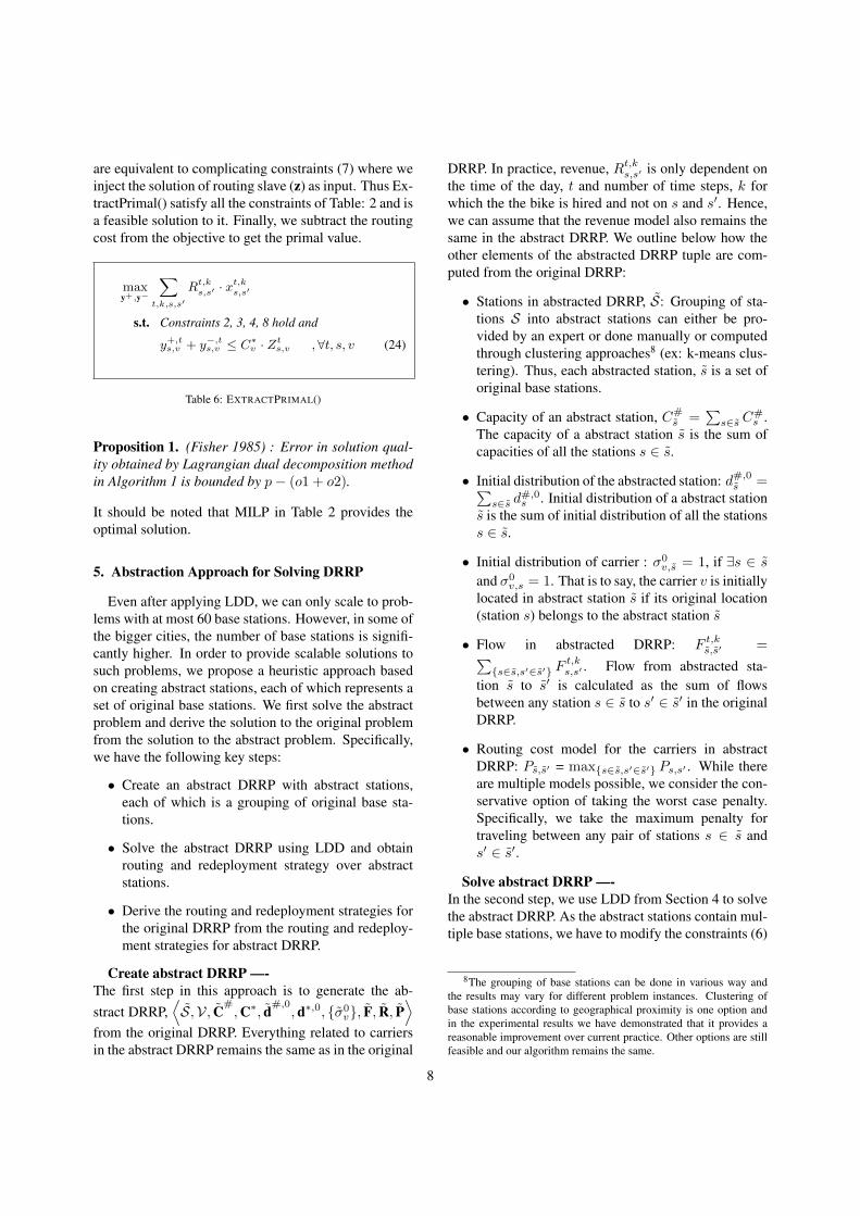
are equivalent to complicating constraints (7) where weinject the solution of routing slave (z) as input. Thus Ex-tractPrimal() satisfy all the constraints of Table: 2 and isa feasible solution to it. Finally, we subtract the routingcost from the objective to get the primal value.

maxy+,y−

∑t,k,s,s′

Rt,ks,s′ · xt,ks,s′

s.t. Constraints 2, 3, 4, 8 hold and

y+,ts,v + y−,ts,v ≤ C∗v · Zts,v ,∀t, s, v (24)

Table 6: EXTRACTPRIMAL()

Proposition 1. (Fisher 1985) : Error in solution qual-ity obtained by Lagrangian dual decomposition methodin Algorithm 1 is bounded by p− (o1 + o2).

It should be noted that MILP in Table 2 provides theoptimal solution.

5. Abstraction Approach for Solving DRRP

Even after applying LDD, we can only scale to prob-lems with at most 60 base stations. However, in some ofthe bigger cities, the number of base stations is signifi-cantly higher. In order to provide scalable solutions tosuch problems, we propose a heuristic approach basedon creating abstract stations, each of which represents aset of original base stations. We first solve the abstractproblem and derive the solution to the original problemfrom the solution to the abstract problem. Specifically,we have the following key steps:

• Create an abstract DRRP with abstract stations,each of which is a grouping of original base sta-tions.

• Solve the abstract DRRP using LDD and obtainrouting and redeployment strategy over abstractstations.

• Derive the routing and redeployment strategies forthe original DRRP from the routing and redeploy-ment strategies for abstract DRRP.

Create abstract DRRP —-The first step in this approach is to generate the ab-stract DRRP,

⟨S,V, C#

,C∗, d#,0

,d∗,0, {σ0v}, F, R, P

⟩from the original DRRP. Everything related to carriersin the abstract DRRP remains the same as in the original

DRRP. In practice, revenue, Rt,ks,s′ is only dependent on

the time of the day, t and number of time steps, k forwhich the the bike is hired and not on s and s′. Hence,we can assume that the revenue model also remains thesame in the abstract DRRP. We outline below how theother elements of the abstracted DRRP tuple are com-puted from the original DRRP:

• Stations in abstracted DRRP, S: Grouping of sta-tions S into abstract stations can either be pro-vided by an expert or done manually or computedthrough clustering approaches8 (ex: k-means clus-tering). Thus, each abstracted station, s is a set oforiginal base stations.

• Capacity of an abstract station, C#s =

∑s∈s C

#s .

The capacity of a abstract station s is the sum ofcapacities of all the stations s ∈ s.

• Initial distribution of the abstracted station: d#,0s =∑

s∈s d#,0s . Initial distribution of a abstract station

s is the sum of initial distribution of all the stationss ∈ s.

• Initial distribution of carrier : σ0v,s = 1, if ∃s ∈ s

and σ0v,s = 1. That is to say, the carrier v is initially

located in abstract station s if its original location(station s) belongs to the abstract station s

• Flow in abstracted DRRP: F t,ks,s′ =∑

{s∈s,s′∈s′} Ft,ks,s′ . Flow from abstracted sta-

tion s to s′ is calculated as the sum of flowsbetween any station s ∈ s to s′ ∈ s′ in the originalDRRP.

• Routing cost model for the carriers in abstractDRRP: Ps,s′ = max{s∈s,s′∈s′} Ps,s′ . While thereare multiple models possible, we consider the con-servative option of taking the worst case penalty.Specifically, we take the maximum penalty fortraveling between any pair of stations s ∈ s ands′ ∈ s′.

Solve abstract DRRP —-In the second step, we use LDD from Section 4 to solvethe abstract DRRP. As the abstract stations contain mul-tiple base stations, we have to modify the constraints (6)

8The grouping of base stations can be done in various way andthe results may vary for different problem instances. Clustering ofbase stations according to geographical proximity is one option andin the experimental results we have demonstrated that it provides areasonable improvement over current practice. Other options are stillfeasible and our algorithm remains the same.

8

to allow multiple carriers in an abstract station. Table:7provides the modified version of the routing slave tosolve the abstracted DRRP. The modified set of Con-straints (25) ensure that at any time step maximum |s|number of carriers can visit in abstract station s. How-ever, the redeployment slave and master function remainsame. There are two key outputs from LDD: (a) Rede-ployment strategy, y for moving bikes between abstractstations; and (b) Routing strategy, z for moving betweenabstract stations, s at different time steps.

minz

∑t,v,s,s′



zts,i,v

s.t. Constraints 5 & 9 hold∑j∈S,v∈V

zts,j,v ≤ |s|, ∀t, s (25)

Table 7: SOLVEABSTRACTEDROUTING()

Derive Strategies for Original DRRP —-In the third step, we retrieve the solution of DRRP fromabstract station level solution. z is the routing strat-egy obtained by solving the abstract problem, where inzts,v =

∑s′ z

ts,s′,v = 1 entails carrier v is present in

abstract state s at time step t. Table 8 provides the opti-mization model to retrieve the solution for DRRP withthe assumption of carrier travels one station in each timestep. We solve the global MIP SolveDRRP() providedin Table2 with an additional set of constraints (26) thatensure a carrier can only be present in a base station atany time step if the station belongs to the abstract stationwhere the carrier is located in the abstract DRRP solu-tion. It also enforces that the decision variable zts,s′,vcan only be 1 if s ∈ s, s′ ∈ s′ and zts,s′,v = 1. In theMILP of RetrieveDRRP(), we explicitly set the decisionvariables zts,s′,v to 0 if s ∈ s, s′ ∈ s′ and zts,s′,v = 0.Thus RetrieveDRRP() becomes an easier optimizationproblem than SolveDRRP().

maxy+,y−,z

∑t,k,s,s′

Rt,ks,s′ · x

t,ks,s′ −

∑t,v,s,s′

Ps,s′ · zts,s′,v

s.t. Constraints 2- 9 hold and∑s∈s,s′∈s′

zts,s′,v = zts,s′,v ∀s, s′, t, v (26)

Table 8: RETRIEVEDRRP()

5.1. Discussion

As we are abstracting the base stations based on theirrelative distance, all the base stations within an abstractstation are located nearby. So, in reality it is possiblefor a carrier to visit all the base stations of an abstractstation within one time-step. This would be the opti-mization problem provided in Table 3. Abstract versionof this problem can be solved directly using the LDDfrom Section 4. However, the mechanism to retrievethe DRRP solution from abstract station level solutionchanges and is outlined here.

5.1.1. Base station level redeployment solutionWe first compute redeployment strategy, y at the level

of base stations for each carrier over the entire horizonand then compute the routing strategy within each ab-stract station. The optimization problem of Table 9 em-ploys the constants, Z to obtain a base station level re-deployment strategy, y. If s is an original station ands is an abstract station, then let Zt

s = 1, if s ∈ s and∑v z

ts,v = 1. Thus we explicitly specify that redeploy-

ment in a base station s is possible only if it belongs toan abstract station s, where a carrier is present in the ab-stract solution. Our objective function specified in (27)is to maximize the overall revenue of the agency thatimplies maximum number of customers are served. In-tuitively we have the following set of constraints:

1. Flow preservation of bikes in and out of stations:Constraints (28) enforce this by ensuring equiva-lence of the number of bikes at station, s at time,t+ 1 (i.e., d#,t+1

s ) to the sum of bikes at station, sat time, t (i.e., d#,t

s ) and net number of bikes arriv-ing at station s after time step t (i.e.,

∑k,s x

t−k,ks,s −∑

k,s′ xt,ks,s′ ), minus the net number of bikes picked

up from station s (i.e.,[y−,ts − y+,t

s

]).

2. Flow of bikes between any two stations followsthe transition dynamics observed in the data: Con-straints (29) ensure that flow of bikes between anytwo station s and s′ should be less than the productof number of bikes present in the source station sand the transition probability that a bike will movefrom s to s′.

3. Redeployment from/to a station is possible if a car-rier is present in that stations: Constraints (30) en-sure that redeployment from/to a station s is possi-ble only if it belongs to an abstract station where acarrier is present in that time-step (i.e., Zt

s = 1).4. Total bikes redeployed from the base stations of an

abstract station is preserved: Constraints (31) en-sure that total bikes picked up or dropped off by

9

the carrier vehicle v, from all base stations in anabstract station s (i.e.,

∑s∈s|zt

s,v=1[y+,ts −y−,ts ]) is

equal to the number of bikes picked up or droppedoff by the carrier v at time t in the abstractionstation level redeployment strategy (i.e., d∗,t+1

v −d∗,tv ).

5. Station capacity is not violated during redeploy-ment: Constraints (32) limit the number of bikespresent in a station s to be less than its capacity(i.e., C#

s ).

maxy+,y−

∑t,s,s,s′

Rt,ks,s′ · xt,ks,s′ (27)

s.t. d#,ts +∑k,s


xt,ks,s′

+ y−,ts − y+,ts = d#,t+1s ,∀t, s (28)


F t,ks,s′∑k,s F

t,ks,s

, ∀t, k, s, s′ (29)

y+,ts + y−,ts ≤ C∗v · Zts ,∀t, s (30)∑s∈s|zts,v=1

[y+,ts − y−,ts ] = d∗,t+1v − d∗,tv , ∀t, s

(31)

0 ≤ xt,ks,s′ ≤ Ft,ks,s′ , y

+,ts , y−,ts ≤ C∗v , d#,ts ≤ C#

s

(32)

Table 9: GETSTATIONREDEPLOY(v,Z, d∗v)

5.1.2. Base station level routing solutionThough the exact redeployment policy is already

known to us, it is important to find the exact routingpolicy of the carriers within each abstract station. Ourgoal is to find the best route within the abstract stationthat should obey the redeployment policy known to usand visit each station only once. We need to considertwo types of route (a) The best route within the abstractstation (i.e. intra-abstract station route) (b) The short-est route among the abstract stations (i.e. inter-abstractstation route).

Given the base station level redeployment strategy, Y(= y), we now compute the best route within the sta-tions of an abstract station, s, while visiting each basestation once and satisfying the redeployment numbersfrom each station, Y. This problem can be solved lo-cally for each abstract station, s, where carrier v is re-deploying at time step t. Thus, if we have |T | time-step

and |V| carriers, we can solve |T | · |V| subproblems sep-arately to get the intra-abstract station routing.

To figure out the initial location, we find a stationwithin the abstract state which is nearest to the stationfrom where the carrier has exited in the previous time-step. Since the position of carriers are known at firsttime step, we can always obtain the starting location.Furthermore, this incremental method will also mini-mize the inter-abstract station routing.

Table 10 provides the optimization problem to solveeach subproblem of the intra-abstract station routing.The objective ( delineated in 33) is to minimize the rout-ing cost of the carrier. The constraints are defined asfollows:

1. Flow of bikes in and out of a carrier is preserved:Constraints (34) enforce this by ensuring the equiv-alence between number of bikes present in the car-rier at time t + 1 to the sum of bikes present inthe carrier at time t and number of bikes pickedup from a station s at that time step (i.e., Y +

s −Y −s |

∑s′ z

ts,s′ = 1).

2. Each station is visited only once: Constraints (35)restrict that each base station where a redeploy-ment is required (i.e. Y +

s /Ys > 0) is visited onlyonce.

3. Flow preservation of carrier in and out of a sta-tion: Constraints (36) ensure that the flow in to astation s (i.e.,

∑s′ z

t−1s′,s ) and flow out from that

station at time t (i.e.,∑

s′ zts,s′ ) are equal. σ0 rep-

resent the initial location of the carrier so that thecarrier moves appropriately from the initial loca-tion.

4. Capacity of the carrier vehicle is not exceeded dur-ing redeployment: Constraints (37) ensure that thenumber of bikes picked up or dropped off by thecarrier in aggregate does not exceed the capacityof the carrier (i.e. C∗v ).

Example 5.1. Figure 4 provides an example to illus-trate the abstraction method where a carrier can coverall stations within an abstract station in one time step.Solid circles represent the base stations and big circlesrepresent the abstract stations. We consider a problemwith 13 base stations and grouped them into threeabstract stations (with 5 stations in abstract station1 and 4 stations each in abstract stations 2 and 3).Initial location of a carrier is indicated with a circleover the solid circle. Figure 4a depicts the optimalabstract station level routing solution (by solving theLDD based global MIP on the abstract DRRP) for thecarrier. Figure 4b depicts the base station level routing

10

minz

∑t,s,s′

Ps,s′ · zts,s′ (33)

s.t. d∗,t +∑s

(Y +s − Y −s ) ·

∑s′

zts,s′

= d∗,t+1 , ∀t ∈ T (34)∑t,s′

zts,s′ = 1 , ∀s ∈ s|(Y +s + Y −s ) > 0 (35)

∑s′

zts,s′ −∑s

zt−1s,s = σt(s) , ∀t ∈ T , s ∈ s

(36)

0 ≤ d∗,t ≤ C∗v , zts,s′ ∈ {0, 1} (37)

Table 10: GETINTRAROUTING(s,Y)

policy within the abstract station 1 at initial time step.It also shows the route from the exit station of abstractstation 1 to its nearest station in abstract station 2. Bythis incremental process we find the base station levelrouting policy for the carriers. Figure 4c, 4d depictsthe base station level routing policy within abstractstation 2 and 3 respectively.

6. Experimental Settings

In this section, we evaluate our approaches with re-spect to run-time, profit, revenue for company and lostdemand on real world9 and synthetic data sets . Thesedata sets contain the following data: (1) Customertrip history records that provide information aboutsuccessful bike booking. We predict the actual demandfrom this trip history. (2) Total number of activedocks in each station (i.e. station capacity) and initialdistribution of bikes in the station at the beginning ofa day. (3) Geographical location of the stations. Fromthe longitude and latitude information of stations, wecalculate the relative distance between two stations. (4)Revenue model of the agency10. (5) Overestimation (toconsider the worst case) of the cost of fuel for carriers11.

9Data is from two leading bike sharing companies in US: Cap-italBikeShare [http://capitalbikeshare.com/system-data] and Hubway[http://hubwaydatachallenge.org/trip-history-data]

10Typically, first 30 minutes for subscription rides is free. Afterthat money is charged. In our model, to ensure consistency, we canrepresent revenue for first 30 minutes as the subscription fees dividedby the average number or rides.

11Mileage results are shown in Table 2 of Fishman et al.(2014) and http://www.globalpetrolprices.com/diesel prices/#USA,

We generated our synthetic data set as follows: (a)We take a subset of the stations from the real world dataset (b) Customer demands, station capacity, geographi-cal location of stations and initial distribution are drawnfrom the real world data for those specific stations. (b)We take the same revenue and cost model discussed ear-lier from real datasets. We employ synthetic data sets toprimarily illustrate the performance benefits providedby LDD over basic MILP based solution. This is be-cause both LDD and MILP are unable to solve problemsat the scale of the real world data sets.

To the best of our knowledge, there is no other ap-proach that addresses this problem nor does there existan approach that can easily be adapted to solve our prob-lem. Hence we compare our approaches against currentpractice of redeploying at the end of the day (in whichuser activities during the rebalancing period are negli-gible) with respect to: (a) overall revenue generated forthe agency; and (b) lost demand.

6.1. Simulating Flow of BikesIn this section we describe the simulation model (that

represents the flow of bikes in the real world) employedto determine how bikes flow between base stations.F t,ks,s′ denotes the outgoing demand from station s to s′ at

time t and d#,ts is the number of bikes present is station

s at time t. The flow of bikes is determined based on thefollowing two cases: (a) If total outflow from a base sta-tion (demand) is less than the number of bikes present inthe base station, then all the customers are served. (b) Iftotal outflow from a a station is higher than the numberof bikes present in the base station, then actual flow (de-

noted as xt,ks,s′ ) depends on the relative ratioF t,k

s,s′∑s′,k F t,k

s,s′.

xt,ks,s′ =

F t,ks,s′ if

∑k,s′ F

t,ks,s′ ≤ d#,t

sF t,k

s,s′∑k,s F t,k

s,s

· d#,ts Otherwise

We calculate the number of bikes present in a station attime t + 1 (see eqn: 38)as the sum of left out bikes attime t and net incoming bikes in that time-step.

d#,t+1s = d#,t

s +[∑

k,s


xt,ks,s′

](38)

So, in each time-step we determines the actual flow ofbikes and then with that information we generate thedistribution of bikes in the next time-step.

shows that diesel price is 1.01 USD per liter, but we overestimate it as1.5 USD to include the cost for extra resource (ex: petrol) consump-tion.

11

T=1 T=2T=0

Abstract_station 1Abstract_station 2 Abstract_station 3

(a)

T=0 T=1 T=2

Abstract_station 1Abstract_station 2

Abstract_station 3

(b)

T=0T=1 T=2

Abstract_station 1Abstract_station 2

Abstract_station 3

(c)

T=0T=1 T=2

Abstract_station 2Abstract_station 3Abstract_station 1

(d)

Figure 4: Routing solution in Abstracted DRRP: (a) Abstract station level routing solution (b) Routing solution within abstract station 1 (c) Routingsolution within abstract station 2 (d) Routing solution within abstract station 3

6.2. Benchmark Approach: Current PracticeAs indicated earlier, currently, the bike sharing sys-

tems redeploy bikes only at the end of the day. We com-pare our approaches against this current practice of notredeploying bikes during the day. Using the simulationmodel described in Section 6.1, we compute the flow ofbikes when no redeployment is done and use that flowinformation to calculate the revenue and lost demand.

Since, we use the simulation approach of Section 6.1to also evaluate the redeployment strategy computedby our decomposition and abstraction approaches, thecomparison against current practice is fair.

7. Experimental Results

We have three sets of results12 on the synthetic dataset. Firstly, we compare the runtime performance ofLDD (SOLVELDD()) with the global MILP (SOLVE-DRRP()) in Figure 5b. X-axis denotes the scale of theproblem where we varied the number of stations from5 to 50. Y-axis denotes the total time taken in secondson a logarithmic scale. Except on small scale problems(ex: 5-10 stations), LDD outperforms global MILP withrespect to runtime. More specifically, global MILP was

12All the linear optimization models were solved using the commer-cial optimization software CPLEX incorporating within python codeon a 3.2 GHz Intel Core i5 machine with 4GB DDR3 RAM

unable to finish within a cut-off time of 6 hours for anyproblem with more than 20 stations, while LDD wasable to solve problems with 50 stations in an hour.

In the second set of results we demonstrate the con-vergence of LDD. LDD can achieve the optimal solutionif the duality gap i.e. the gap between primal and dualsolution becomes zero. Figure 5a shows that the dualitygap for a 20 station problem is only 1%. Figure 5c,5ddepict the duality gap for real world data set of Hubway(with 95 base stations and grouped in 25 abstract sta-tions) and CapitalBikeShare (with 305 base stations andgrouped into 50 abstract stations) respectively. For bothof these larger problems we are able to get a solutionwith duality gap of less than 0.5 %.

Finally, we demonstrate the performance of abstrac-tion in comparison with optimal on a problem with 30base stations. We grouped those 30 base stations into8 abstract stations. Then we run the LDD based opti-mization on both the base station and abstraction stationproblems. Table 11 shows the effect of abstraction onthe generated revenue and execution time based on fiverandom instances of customer demand. Although, thereis only a reduction of 0.2% on average from optimal, itgives a significant computational gain.

Capital-Bikeshare Results ——The majority of our results are provided on the Capital-BikeShare dataset. The data set has 305 active stationsand we consider 50 abstract stations (obtained through

12

Figure 5: (a) Duality gap in synthetic dataset with 20 station (b) Runtime: LDD vs Global MILP (c) Duality gap in Hubway dataset (d) Duality gapin CapitalBikeshare dataset

WithAbstraction

WithoutAbstraction

Instance Revenue Runtime(sec) Revenue Runtime

(sec)1 23580 51 23640 38402 23627 106 23678 35403 23610 57 23727 31204 23613 49 23645 31505 23519 45 23590 3119

Table 11: Effect of Abstraction

k-means clustering). The planning horizon is 38 ( 30minute intervals during the working hours from 5AM-12AM).

We now provide the performance comparison be-tween our approaches and current practice (i.e., no re-deployment during the day) with respect to lost demandand revenue generated for the bike-sharing company.We generate the overall mean demand as well as thedemand for individual weekdays from historical data oftrips. We compute the results for the entire time hori-

zon (from 5 AM to 12 AM) and also for one of the peakduration (from 5 AM to 12 PM). We consider the triphistory data of four quarters of 2013 and for each quar-ter we have done the same set of experiments. Table12shows the percentage gain in revenue and the percent-age reduction in lost demand in comparison with currentpractice for the first quarter. With respect to both rev-enue gain and lost demand, our approach (abstraction +LDD + MILP) was able to outperform current practiceduring the peak time as well as during the day. We re-duce the lost demand in all the cases by at least 15%,a significant improvement over current practice. As ex-pected, for all of those instances, the percentage revenuegain in the peak hours is much higher because most ofthe lost demands occurs in the peak hours.

Table13 shows the percentage gain in revenue and thepercentage reduction in lost demand in comparison withcurrent practice for the second quarter. Our approachis able to reduce the lost demand in all the cases by atleast 10%, while the revenue is improved by an averageof 3%.

Table14 shows the comparison with current practice

13

Whole day(5am-12am)

Peak period(5am-12pm)

Revenuegain

Lostdemand

reduction

Revenuegain

Lostdemand

reductionMean 2.11 % 23.4 % 2.92 % 17.16 %Mon 1.33 % 23.18 % 6.57 % 35.11 %Tue 1.91 % 26.33 % 6.63 % 35.37 %Wed 2.19 % 29.26 % 8.13 % 39.68 %Thu 2.5 % 30.66 % 7.63 % 38.5 %Fri 2.43 % 31.27 % 7.22 % 37.46 %Sat 1.34 % 15.1 % 1.08 % 22.91 %Sun 1.01 % 15.44 % 0.49 % 14.63 %

Table 12: Revenue and lost demand comparison (Dataset: Capital-Bikeshare, 1st quarter of 2013)

Whole day(5am-12am)


Revenuegain

Lostdemand

reduction

Revenuegain

Lostdemand


Table 13: Revenue and lost demand comparison (Dataset: Capital-Bikeshare, 2nd quarter of 2013)

for the third quarter (busiest quarter in the year). For thisquarter, our approach is able to reduce the lost demandin all the cases by at least 22%, while the revenue isimproved by at least 3%.

Table15 shows the percentage gain in revenue and thepercentage reduction in lost demand in comparison withcurrent practice for the last quarter. For this data set,our approach reduces the lost demand by at least 10%over current practice. For all of those quarters, the per-centage revenue gain in the peak hours is almost doublebecause most of the lost demands occur in these time-period.

The next set of results demonstrate the sensitivityof our approach with respect to small variations in de-mand. We created a set of 10 demands for each of theweekdays from the underlying poisson distribution withmean calculated from the real world data set. For indi-vidual demand instances, we calculate the revenue andlost demand by applying our redeployment policy and

Whole day(5am-12am)


Revenuegain

Lostdemand

reduction

Revenuegain

Lostdemand


Table 14: Revenue and lost demand comparison (Dataset: Capital-Bikeshare, 3rd quarter of 2013)

Whole day(5am-12am)


Revenuegain

Lostdemand

reduction

Revenuegain

Lostdemand


Table 15: Revenue and lost demand comparison (Dataset: Capital-Bikeshare, 4th quarter of 2013)

compare it with the current practice. Figure 6 show themean and deviation of the revenue and lost demand forthe first quarter. Even considering the variance, Fig-ure 6a depict that the revenue generated by followingour redeployment strategy for each of the weekdays isstill better (albeit by a small amount) than current prac-tice. Figure 6b demonstrate that we are able to sig-nificantly reduce the lost demand on all the cases. Itis interesting to note that the gain in weekdays (Mon-Fri) is significantly high because of a consistent patternin customer demand. While in weekends, the demandmay vary abruptly and the performance gain for all re-alization of demand is poor.

Figure 7 shows the mean and deviation of the revenueand lost call for the second quarter. Figure 7a depictsthat the revenue generated by following our redeploy-ment strategy for each of the weekdays is better thancurrent practice. More interestingly, Figure 7b showsthat we are able to significantly reduce the lost demand

14

Figure 6: Sensitivity analysis [Dataset: CapitalBikeShare, 1st quarter of 2013]: (a) Revenue comparison (b) Lost demand comparison

Figure 7: Sensitivity analysis [Dataset: CapitalBikeShare, 2nd quarter of 2013]: (a) Revenue comparison (b) Lost demand comparison

on all the instances.Finally, we provide the mean and deviation of the rev-

enue and lost call for the third and fourth quarter in Fig-ure 8,9 respectively. Even considering the variance, Fig-ure 8a,9a depict that the revenue generated by followingour redeployment strategy for each of the weekdays isstill better than current practice. Figure 8b,9b demon-strate that we are able to significantly reduce the lostdemand on all the cases.

Hubway Results ——Now we present the results on the real world dataset ofHubway. Hubway BSS comprises with 95 active sta-tions and we group them into 25 abstract stations. Wetake two quarters (2nd and 3rd quarter of 2012) of triphistory data into our consideration. Similar to the pre-vious data set, we generate the overall mean demand aswell as the demand for individual weekdays from his-torical data of trips.

We produce two sets of results with this data set. Ta-ble 16 provide the comparison results (on revenue andlost demand) for the third quarter. Our approach is able

to gain an excess 5% in revenue on average while thelost demand is reduced by a minimum of 40 %.

WithoutRede-

ployment

WithRede-

ploymentGain(%)

Reve-nue

Lostde-

mand

Reve-nue

Lostde-

mand

Reve-nue

Lostde-

mandMean 5867 341 6342 92 8.10 73.02Mon 6122 312 6363 179 3.94 42.63Tue 5701 308 6039 121 5.93 60.71Wed 6025 258 6293 107 4.45 58.53Thu 6029 351 6385 159 5.90 54.70Fri 5567 251 5916 57 6.27 77.29Sat 6726 93 6874 28 2.20 69.89Sun 6447 100 6650 26 3.15 74.00

Table 16: Revenue and lost demand comparison (Hubway, Dataset:3-rd quarter of 2012 )

15

Figure 8: Sensitivity analysis [Dataset: CapitalBikeShare, 3rd quarter of 2013]: (a) Revenue comparison (b) Lost demand comparison

Figure 9: Sensitivity analysis [Dataset: CapitalBikeShare, 4th quarter of 2013]: (a) Revenue comparison (b) Lost demand comparison

In Table 17, we provide the percentage gain in rev-enue and the percentage reduction in lost demand incomparison with current practice for the second quar-ter of Hubway Dataset. In this scenario, our approach isable to gain an excess 3% in revenue on average whilethe lost demand is reduced by a minimum of 30 %.

Lastly, to visualize the effect of redeployment wedraw the correlation between actual demand and serveddemand over the planning horizon. Since we aim to re-duce the lost customer demand, it is better if most ofthe points are near to line of equality or identity line.Figure 10b illustrates the correlation between actual de-mand and demand served by following our redeploy-ment model. Comparatively, with redeployment thereare many more points closer to the identity line thanwith current practice (shown in Figure: 10a).

8. Related Work

Given the practical benefits of bike sharing systems,they have been studied extensively in the literature. We

WithoutRede-

ployment

WithRede-

ploymentGain(%)

Reve-nue

Lostde-

mand

Reve-nue

Lostde-

mand

Reve-nue

Lostde-

mandMean 4213 152 4317 106 2.46 30.26Mon 4339 95 4488 30 3.43 68.42Tue 4607 98 4751 33 3.12 66.32Wed 3514 150 3743 40 6.51 73.33Thu 4420 97 4504 61 1.90 37.11Fri 4480 75 4549 42 1.54 44Sat 4679 92 4792 43 2.41 53.26Sun 4086 105 4232 41 3.57 60.95

Table 17: Revenue and lost demand comparison (Hubway, Dataset:2-nd quarter of 2012 )

focus on three threads of research that are of relevance

16

0

0.5

1

1.5

2

2.5

3

3.5

4

0 0.5 1 1.5 2 2.5 3 3.5 4

Ser

ved

Dem

and

Actual Demand

0

0.5

1

1.5

2

2.5

3

3.5

4

0 0.5 1 1.5 2 2.5 3 3.5 4

Ser

ved

Dem

and

Actual Demand

Figure 10: Correlation of demand and supply: (a) Without redeployment (b) With dynamic redeployment

to this paper. First thread of papers focus on the prob-lem of finding routes at the end of the day for a fixed setof carriers to achieve the desired configuration of bikesacross the base stations. Schuijbroek et al. (2013) pro-pose a scalable approximate solution for this problem byabstracting base stations into mega stations and solvedit using a clustered vehicle routing (CluVRP) approach.Benchimol et al. (2011) present an approximate solution(inspired by the solution of C-delivery TSP) to solve thestatic re-balancing and routing problem by consideringa single carrier vehicle. Raviv and Kolka (2013), Ravivet al. (2013) have provided scalable exact and approxi-mate approaches to this routing problem by employinginsights from inventory management. They introduce aset of MILP formulations that solve the static bicyclerepositioning problem (SBRP). They penalize the ob-jective function for unavailability of bikes or open docksand thus find an static redeployment model for the car-riers to rearrange the inventory. Raidl et al. (2013) pro-vide an approximate solution of SBRP by using vari-able neighbourhood search based heuristics. All the pa-pers in this thread assume there is only one fixed rede-ployment of bikes that happens at the end of the day.However, as described in Fricker and Gast (2012) andas demonstrated in our experimental results section, notperforming redeployment during the day can result in asignificant loss in demand. In contrast, our approachesdiffer from this thread of research as we consider dy-namic redeployment during the day.

The second thread of research focuses on the place-ment of base stations and on performing dynamic re-deployment of bikes during the day. Kumar and Bier-laire (2012) develop a linear regression model to un-derstand the correlation between stations location andcustomers location by analyzing the customers demo-graphic and personal information. In addition, Martinezet al. (2012) provide an MILP formulation to optimally

locate the stations, and solve it using branch and boundalgorithm. Lin and Yang (2011), Lin et al. (2013) pro-pose a decision support model to design and managethe public bicycle sharing (PBS) system. They providea formal model to meet the service level requirementof PBS with the help of well known constraints frominventory or logistic management. Unfortunately, theflow in PBS depends on the stochastic demand or invol-untary movement of customers and this static solutioncan significantly falter. Shu et al. (2013, 2010) predictthe stochastic demand from user trip data of Singaporemetro system using poisson distribution and provide anoptimization model that suggests the best location ofthe stations and a dynamic redeployment model to mini-mize the number of unsatisfied customer. However, theyassume that redeployment of bikes from one station toanother is always possible without considering the rout-ing of carriers, which is a major cost driver for the bike-sharing company. Chemla et al. (2013) solve the staticre-balancing problem by considering a single carrierand provide a branch and cut algorithm that can solvea large scale problem with more than hundred stations.Contardo et al. (2012) propose a dynamic redeploymentmodel to deal with unmet demand in rush hours. Theyprovide a myopic redeployment policy by consideringthe current demand. They employed Dantzig-Wolfe andBenders decomposition techniques to make the decisionproblem faster. Though due to the complex structure ofthe problem there was a significant gap between theirsolution and its lower bound. As can be observed fromthe data, customer demand of bikes varies over timestochastically and hence a myopic redeployment pol-icy can significantly falter as it does not consider thefuture demand. Our approaches differ from this threadof research as we consider dynamic redeployment androuting of carriers together and consider the multi-stepexpected demand in determining the dynamic redeploy-

17

ment policy.The third thread of research which is complemen-

tary to the work presented in this paper is on demandprediction and analysis. We have already highlightedthe assumption that demand follows poisson distribu-tion employed by Shu et al. (2013, 2010). Nair andMiller-Hooks (2011), Nair et al. (2013) provide a ser-vice level analysis of the Bike Sharing System using adual-bounded joint-chance constraints where they pre-dict the near future demands for a short period and makesure that all the system wide demands should be servedwith a certain probability. While, this may not be ap-plicable for a large system with a small set of carri-ers, the insights generated are practical and useful indemand prediction. Leurent (2012) report the bike shar-ing system as a dual markovian waiting system to pre-dict the actual demand. Froehlich et al. (2008), Lathiaet al. (2012) predict the temporal user demand in termsof available bicycles or normalized available bicycle(NAB) in a station at a certain time step. Given its gen-erality and can be employed over an entire horizon, wealso employ the demand prediction model employed byShu et al. (2013, 2010) and assume that demand fol-lows a poisson distribution. However, the parameter, λthat governs the poisson distribution is learned from realdata.

9. Conclusion

In this paper we address the dynamic redeploy prob-lem in shared transportation systems. Our approachbased on the Lagrangian Dual Decomposition and anabstraction based mechanism, addresses two key chal-lenges (a) Provide an near-optimal policy for the dy-namic redeployment of idle vehicles in conjunction withthe routing solution for carriers (b) Provide a scalablesolution for the real-world large scale problems. Theempirical results on multiple real and synthetic data setsshown that our dynamic redeployment approach is notonly able to achieve the original goal of reducing lostdemand, but is also able to improve revenue for the bikesharing company, by using their existing resources. Infuture this work can be extended with a robust optimiza-tion technique which can account for all the realizationof different demand scenarios.

Acknowledgments

The research described in this paper was funded inpart by the Singapore National Research Foundation

(NRF) through the Singapore-MIT Alliance for Re-search and Technology (SMART) Center for FutureMobility (FM).

References

C. Fricker, N. Gast, Incentives and redistribution in homoge-neous bike-sharing systems with stations of finite ca-pacity, EURO Journal on Transportation and Logistics(2012) 1–31.

J. D. Lees-Miller, J. C. Hammersley, R. E. Wilson, Theoreti-cal maximum capacity as benchmark for empty vehicleredistribution in personal rapid transit, TransportationResearch Record: Journal of the Transportation Re-search Board 2146 (1) (2010) 76–83.

Y. Yue, L. Marla, R. Krishnan, An Efficient Simulation-BasedApproach to Ambulance Fleet Allocation and DynamicRedeployment., in: AAAI, 2012.

S. Saisubramanian, P. Varakantham, L. H. Chuin, Risk basedOptimization for Improving Emergency Medical sys-tems., in: AAAI, 2015.

J. Schuijbroek, R. Hampshire, W.-J. van Hoeve, Inventory re-balancing and vehicle routing in bike sharing systems,Working Paper, Carnegie Mellon University .

J. Shu, M. C. Chou, Q. Liu, C.-P. Teo, I.-L. Wang, Modelsfor effective deployment and redistribution of bicycleswithin public bicycle-sharing systems, Operations Re-search 61 (6) (2013) 1346–1359.

M. L. Fisher, An applications oriented guide to Lagrangianrelaxation, Interfaces 15 (2) (1985) 10–21.

G. J. Gordon, P. Varakantham, W. Yeoh, H. C. Lau, A. S.Aravamudhan, S.-F. Cheng, Lagrangian relaxation forlarge-scale multi-agent planning, in: Web Intelligenceand Intelligent Agent Technology (WI-IAT), 2012IEEE/WIC/ACM International Conferences on, vol. 2,IEEE, 494–501, 2012.

E. Fishman, S. Washington, N. L. Haworth, Bike share’s im-pact on car use: evidence from the United States, GreatBritain, and Australia, in: Proceedings of the 93rd An-nual Meeting of the Transportation Research Board,2014.

M. Benchimol, P. Benchimol, B. Chappert, A. De La Taille,F. Laroche, F. Meunier, L. Robinet, Balancing thestations of a self service bike hire system, RAIRO-Operations Research 45 (01) (2011) 37–61.

T. Raviv, O. Kolka, Optimal inventory management of a bike-sharing station, IIE Transactions 45 (10) (2013) 1077–1093.

T. Raviv, M. Tzur, I. A. Forma, Static repositioning in abike-sharing system: models and solution approaches,EURO Journal on Transportation and Logistics 2 (3)(2013) 187–229.

18

G. R. Raidl, B. Hu, M. Rainer-Harbach, P. Papazek, Balanc-ing bicycle sharing systems: Improving a VNS by effi-ciently determining optimal loading operations (2013)130–143.

V. P. Kumar, M. Bierlaire, Optimizing locations fora vehicle sharing system, in: Swiss Trans-port Research Conference. http://www. strc.ch/conferences/2012/Kumar Bierlaire. pdf, 2012.

L. M. Martinez, L. Caetano, T. Eiro, F. Cruz, An optimisa-tion algorithm to establish the location of stations of amixed fleet biking system: an application to the cityof Lisbon, Procedia-Social and Behavioral Sciences 54(2012) 513–524.

J.-R. Lin, T.-H. Yang, Strategic design of public bicycle shar-ing systems with service level constraints, Transporta-tion research part E: logistics and transportation review47 (2) (2011) 284–294.

J.-R. Lin, T.-H. Yang, Y.-C. Chang, A hub location inven-tory model for bicycle sharing system design: Formula-tion and solution, Computers & Industrial Engineering65 (1) (2013) 77–86.

J. Shu, M. Chou, Q. Liu, C.-P. Teo, I.-L. Wang, Bicycle-sharing system: deployment, utilization and the valueof re-distribution, National University of Singapore-NUS Business School, Singapore .

D. Chemla, F. Meunier, R. Wolfler Calvo, Bike sharing sys-tems: Solving the static rebalancing problem, DiscreteOptimization 10 (2) (2013) 120–146.

C. Contardo, C. Morency, L.-M. Rousseau, Balancing a dy-namic public bike-sharing system, vol. 4, CIRRELT,2012.

R. Nair, E. Miller-Hooks, Fleet management for vehicle shar-ing operations, Transportation Science 45 (4) (2011)524–540.

R. Nair, E. Miller-Hooks, R. C. Hampshire, A. Busic, Large-Scale Vehicle Sharing Systems: Analysis of Velib’, In-ternational Journal of Sustainable Transportation 7 (1)(2013) 85–106.

F. Leurent, Modelling a vehicle-sharing station as a dual wait-ing system: stochastic framework and stationary analy-sis .

J. Froehlich, J. Neumann, N. Oliver, Measuring the pulse ofthe city through shared bicycle programs, Proc. of Ur-banSense08 (2008) 16–20.

N. Lathia, S. Ahmed, L. Capra, Measuring the impact of open-ing the London shared bicycle scheme to casual users,Transportation research part C: emerging technologies22 (2012) 88–102.

19

dynamic redeployment to reduce lost demand in vehicle

Documents