dynamic programming - university of minnesota · dynamic programming the dependencies between...

Dynamic Programming

Ananth Grama, Anshul Gupta, George Karypis, and Vipin Kumar

To accompany the text “Introduction to Parallel Computing”,Addison Wesley, 2003.

Topic Overview

• Overview of Serial Dynamic Programming

• Serial Monadic DP Formulations

• Nonserial Monadic DP Formulations

• Serial Polyadic DP Formulations

• Nonserial Polyadic DP Formulations

– Typeset by FoilTEX – 1

Overview of Serial Dynamic Programming

• Dynamic programming (DP) is used to solve a wide varietyof discrete optimization problems such as scheduling, string-editing, packaging, and inventory management.

• Break problems into subproblems and combine their solutionsinto solutions to larger problems.

• In contrast to divide-and-conquer, there may be relationshipsacross subproblems.


Dynamic Programming: Example

• Consider the problem of finding a shortest path between a pairof vertices in an acyclic graph.

• An edge connecting node i to node j has cost c(i, j).

• The graph contains n nodes numbered 0, 1, . . . , n − 1, and hasan edge from node i to node j only if i < j. Node 0 is sourceand node n − 1 is the destination.

• Let f(x) be the cost of the shortest path from node 0 to nodex.

f(x) =

{

0 x = 0min

0≤j<x{f(j) + c(j, x)} 1 ≤ x ≤ n − 1


Dynamic Programming: Examplec(0,1)

c(2,3)c(1,2)

c(1,3)

c(2,4)c(0,2)

c(3,4)1 3

2

40

A graph for which the shortest path between nodes 0 and 4 is tobe computed.

f(4) = min{f(3) + c(3, 4), f(2) + c(2, 4)}.


Dynamic Programming

• The solution to a DP problem is typically expressed as aminimum (or maximum) of possible alternate solutions.

• If r represents the cost of a solution composed of subproblemsx1, x2, . . ., xl, then r can be written as

r = g(f(x1), f(x2), . . . , f(xl)).

Here, g is the composition function.

• If the optimal solution to each problem is determined bycomposing optimal solutions to the subproblems and selectingthe minimum (or maximum), the formulation is said to be a DPformulation.


Dynamic Programming: Example

Composition of solutions into a term

Minimization of terms

PSfrag replacements

f(x1)

f(x2)

f(x3)

f(x4)

f(x5)

f(x6)

f(x7)

r1 = g(f(x1), f(x3))

r2 = g(f(x4), f(x5))

r3 = g(f(x2), f(x6), f(x7))

f(x8) = min{r1, r2, r3}

The computation and composition of subproblem solutions tosolve problem f(x8).


Dynamic Programming

• The recursive DP equation is also called the functional equationor optimization equation.

• In the equation for the shortest path problem the compositionfunction is f(j) + c(j, x). This contains a single recursive term(f(j)). Such a formulation is called monadic.

• If the RHS has multiple recursive terms, the DP formulation iscalled polyadic.


Dynamic Programming

• The dependencies between subproblems can be expressed asa graph.

• If the graph can be levelized (i.e., solutions to problems ata level depend only on solutions to problems at the previouslevel), the formulation is called serial, else it is called non-serial.

• Based on these two criteria, we can classify DP formulationsinto four categories – serial-monadic, serial-polyadic, non-serial-monadic, non-serial-polyadic.

• This classification is useful since it identifies concurrency anddependencies that guide parallel formulations.


Serial Monadic DP Formulations

• It is difficult to derive canonical parallel formulations for theentire class of formulations.

• For this reason, we select two representative examples, theshortest-path problem for a multistage graph and the 0/1knapsack problem.

• We derive parallel formulations for these problems and identifycommon principles guiding design within the class.


Shortest-Path Problem

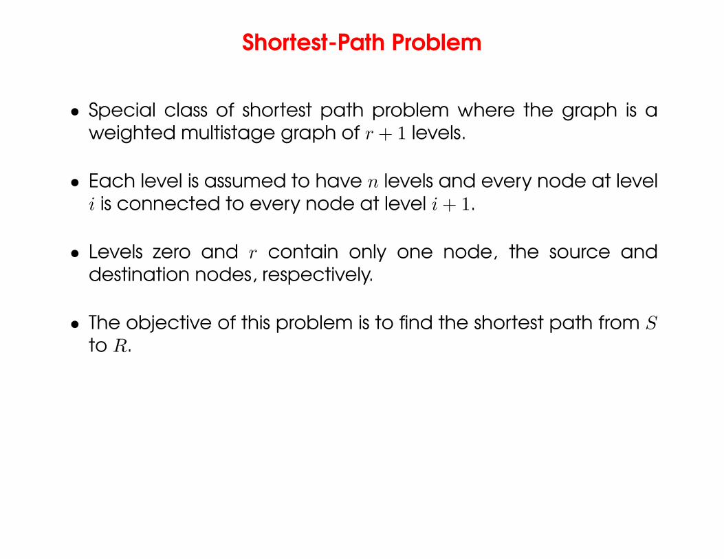
• Special class of shortest path problem where the graph is aweighted multistage graph of r + 1 levels.

• Each level is assumed to have n levels and every node at leveli is connected to every node at level i + 1.

• Levels zero and r contain only one node, the source anddestination nodes, respectively.

• The objective of this problem is to find the shortest path from Sto R.


Shortest-Path Problem

PSfrag replacements

S

c0S,0

c0S,2

c0S,n−1

c10,0

c1n−1,n−1

c20,0

c2n−1,n−1

cr−10,R

cr−1n−1,R

R

v10

v11

v12

v1n−1

v20

v2n−1

v30

v3n−1

vr−10

vr−1n−1

An example of a serial monadic DP formulation for finding the shortest path ina graph whose nodes can be organized into levels.


Shortest Path Problem

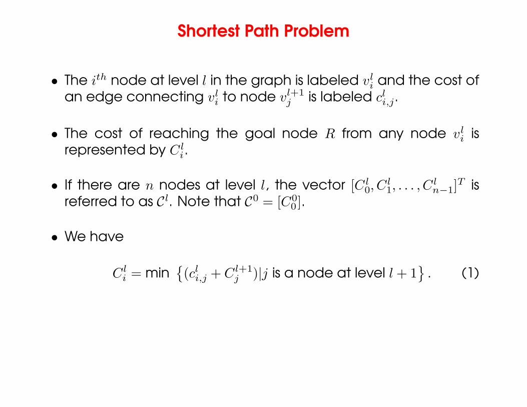
• The ith node at level l in the graph is labeled vli and the cost of

an edge connecting vli to node vl+1

j is labeled cli,j.

• The cost of reaching the goal node R from any node vli is

represented by C li.

• If there are n nodes at level l, the vector [C l0, C

l1, . . . , C

ln−1]

T isreferred to as Cl. Note that C0 = [C0

0 ].

• We have

Cli = min

{

(cli,j + Cl+1

j )|j is a node at level l + 1}

. (1)



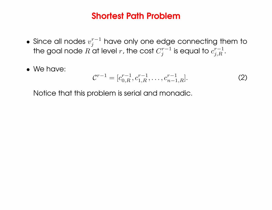
• Since all nodes vr−1j have only one edge connecting them to

the goal node R at level r, the cost Cr−1j is equal to cr−1

j,R .

• We have:Cr−1 = [cr−1

0,R , cr−11,R , . . . , cr−1

n−1,R]. (2)

Notice that this problem is serial and monadic.



The cost of reaching the goal node R from any node at level l(0 < l < r − 1) is

Cl0 = min{(cl

0,0 + Cl+10 ), (cl

0,1 + Cl+11 ), . . . , (cl

0,n−1 + Cl+1n−1)},

Cl1 = min{(cl

1,0 + Cl+10 ), (cl

1,1 + Cl+11 ), . . . , (cl

1,n−1 + Cl+1n−1)},

...

Cln−1 = min{(cl

n−1,0 + Cl+10 ), (cl

n−1,1 + Cl+11 ), . . . , (cl

n−1,n−1 + Cl+1n−1)}.



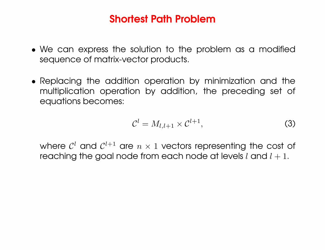
• We can express the solution to the problem as a modifiedsequence of matrix-vector products.

• Replacing the addition operation by minimization and themultiplication operation by addition, the preceding set ofequations becomes:

Cl = Ml,l+1 × Cl+1, (3)

where Cl and Cl+1 are n × 1 vectors representing the cost ofreaching the goal node from each node at levels l and l + 1.



• Matrix Ml,l+1 is an n×n matrix in which entry (i, j) stores the costof the edge connecting node i at level l to node j at level l+1.

•

Ml,l+1 =

cl0,0 cl

0,1 . . . cl0,n−1

cl1,0 cl

1,1 . . . cl1,n−1... ... ...

cln−1,0 cl

n−1,1 . . . cln−1,n−1

.

• The shortest path problem has been formulated as a sequenceof r matrix-vector products.


Parallel Shortest Path

• We can parallelize this algorithm using the parallel algorithmsfor the matrix-vector product.

• Θ(n) processing elements can compute each vector C l in timeΘ(n) and solve the entire problem in time Θ(rn).

• In many instances of this problem, the matrix M may be sparse.For such problems, it is highly desirable to use sparse matrixtechniques.


0/1 Knapsack Problem

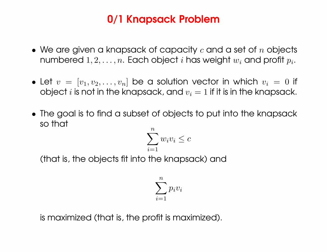
• We are given a knapsack of capacity c and a set of n objectsnumbered 1, 2, . . . , n. Each object i has weight wi and profit pi.

• Let v = [v1, v2, . . . , vn] be a solution vector in which vi = 0 ifobject i is not in the knapsack, and vi = 1 if it is in the knapsack.

• The goal is to find a subset of objects to put into the knapsackso that

n∑

i=1

wivi ≤ c

(that is, the objects fit into the knapsack) and

n∑

i=1

pivi

is maximized (that is, the profit is maximized).



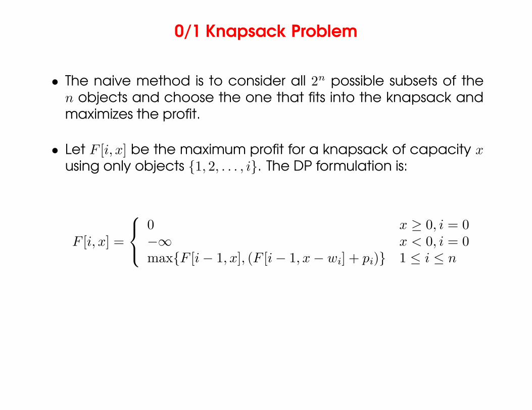
• The naive method is to consider all 2n possible subsets of then objects and choose the one that fits into the knapsack andmaximizes the profit.

• Let F [i, x] be the maximum profit for a knapsack of capacity xusing only objects {1, 2, . . . , i}. The DP formulation is:

F [i, x] =

0 x ≥ 0, i = 0−∞ x < 0, i = 0max{F [i − 1, x], (F [i − 1, x − wi] + pi)} 1 ≤ i ≤ n



• Construct a table F of size n × c in row-major order.

• Filling an entry in a row requires two entries from the previousrow: one from the same column and one from the columnoffset by the weight of the object corresponding to the row.

• Computing each entry takes constant time; the sequential runtime of this algorithm is Θ(nc).

• The formulation is serial-monadic.



1

2

1Weights

Processors

PSfrag replacements

P0

i

n

j cc − 1

Table F

Pj−wi−1 Pj−1 Pc−2 Pc−1

j − wi

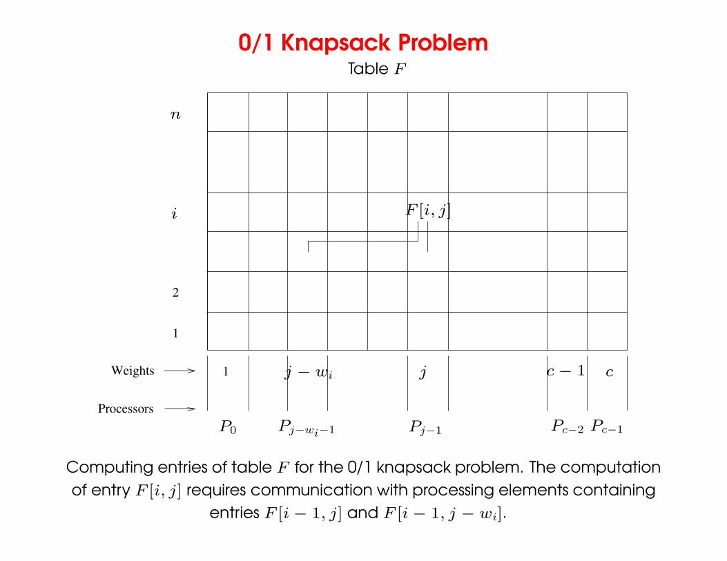
F [i, j]

Computing entries of table F for the 0/1 knapsack problem. The computationof entry F [i, j] requires communication with processing elements containing

entries F [i − 1, j] and F [i − 1, j − wi].



• Using c processors in a PRAM, we can derive a simple parallelalgorithm that runs in O(n) time by partitioning the columnsacross processors.

• In a distributed memory machine, in the jth iteration, forcomputing F [j, r] at processing element Pr−1, F [j − 1, r] isavailable locally but F [j − 1, r − wj] must fetched.

• The communication operation is a circular shift and the time isgiven by (ts+tw) log c. The total time is therefore tc+(ts+tw) log c.

• Across all n iterations (rows), the parallel time is O(n log c). Notethat this is not cost optimal.



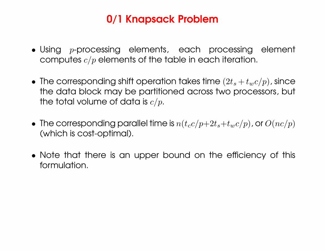
• Using p-processing elements, each processing elementcomputes c/p elements of the table in each iteration.

• The corresponding shift operation takes time (2ts + twc/p), sincethe data block may be partitioned across two processors, butthe total volume of data is c/p.

• The corresponding parallel time is n(tcc/p+2ts+twc/p), or O(nc/p)(which is cost-optimal).

• Note that there is an upper bound on the efficiency of thisformulation.


Nonserial Monadic DP Formulations:Longest-Common-Subsequence

• Given a sequence A = 〈a1, a2, . . . , an〉, a subsequence of A canbe formed by deleting some entries from A.

• Given two sequences A = 〈a1, a2, . . . , an〉 and B =〈b1, b2, . . . , bm〉, find the longest sequence that is a subsequenceof both A and B.

• If A = 〈c, a, d, b, r, z〉 and B = 〈a, s, b, z〉, the longest commonsubsequence of A and B is 〈a, b, z〉.


Longest-Common-Subsequence Problem

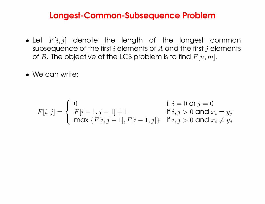
• Let F [i, j] denote the length of the longest commonsubsequence of the first i elements of A and the first j elementsof B. The objective of the LCS problem is to find F [n, m].

• We can write:

F [i, j] =

0 if i = 0 or j = 0F [i − 1, j − 1] + 1 if i, j > 0 and xi = yj

max {F [i, j − 1], F [i − 1, j]} if i, j > 0 and xi 6= yj



• The algorithm computes the two-dimensional F table in a row-or column-major fashion. The complexity is Θ(nm).

• Treating nodes along a diagonal as belonging to one level,each node depends on two subproblems at the precedinglevel and one subproblem two levels prior.

• This DP formulation is nonserial monadic.



(b)(a)

1

2

n

0 0 0 0 0

0

0

0

0

0

0 1 2 m

PSfrag replacements

P0 P1 Pn−1

(a) Computing entries of table F for thelongest-common-subsequence problem. Computationproceeds along the dotted diagonal lines. (b) Mapping

elements of the table to processing elements.


Longest-Common-Subsequence: Example

Consider the LCS of two amino-acid sequences H E A G A W GH E E and P A W H E A E. For the interested reader, the names

of the corresponding amino-acids are A: Alanine, E: Glutamicacid, G: Glycine, H: Histidine, P: Proline, and W: Tryptophan.

H E A G A W G H E E

0 0 0 0 0 0 0 0 0 0 0

P

A

W

0 0 0 0 0 0 0 0 0 0 0

0 0 0 1 1 1 1 1 1 1 1

0 0 0 1 1 1 2 2 2 2 2

H 0 1 1 1 1 1 2 2 3 3 3

E 0 1 2 2 2 2 2 2 3 4 4

A 0 1 2 3 4 43 3 3 3 3

E 0 1 2 3 4 53 3 3 3 3

The F table for computing the LCS of the sequences. The LCS is AW H E E.


Parallel Longest-Common-Subsequence

• Table entries are computed in a diagonal sweep from the top-left to the bottom-right corner.

• Using n processors in a PRAM, each entry in a diagonal can becomputed in constant time.

• For two sequences of length n, there are 2n − 1 diagonals.

• The parallel run time is Θ(n) and the algorithm is cost-optimal.


Parallel Longest-Common-Subsequence

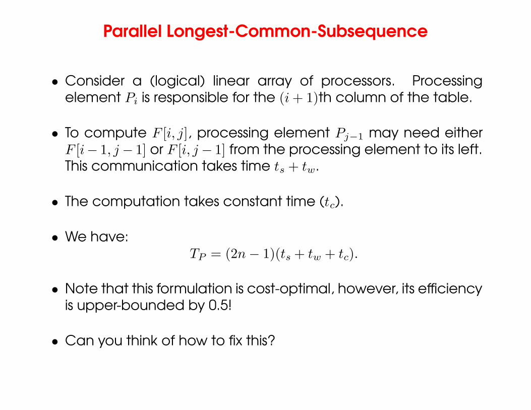
• Consider a (logical) linear array of processors. Processingelement Pi is responsible for the (i + 1)th column of the table.

• To compute F [i, j], processing element Pj−1 may need eitherF [i− 1, j − 1] or F [i, j − 1] from the processing element to its left.This communication takes time ts + tw.

• The computation takes constant time (tc).

• We have:TP = (2n − 1)(ts + tw + tc).

• Note that this formulation is cost-optimal, however, its efficiencyis upper-bounded by 0.5!

• Can you think of how to fix this?


Serial Polyadic DP Formulation: Floyd’s All-PairsShortest Path

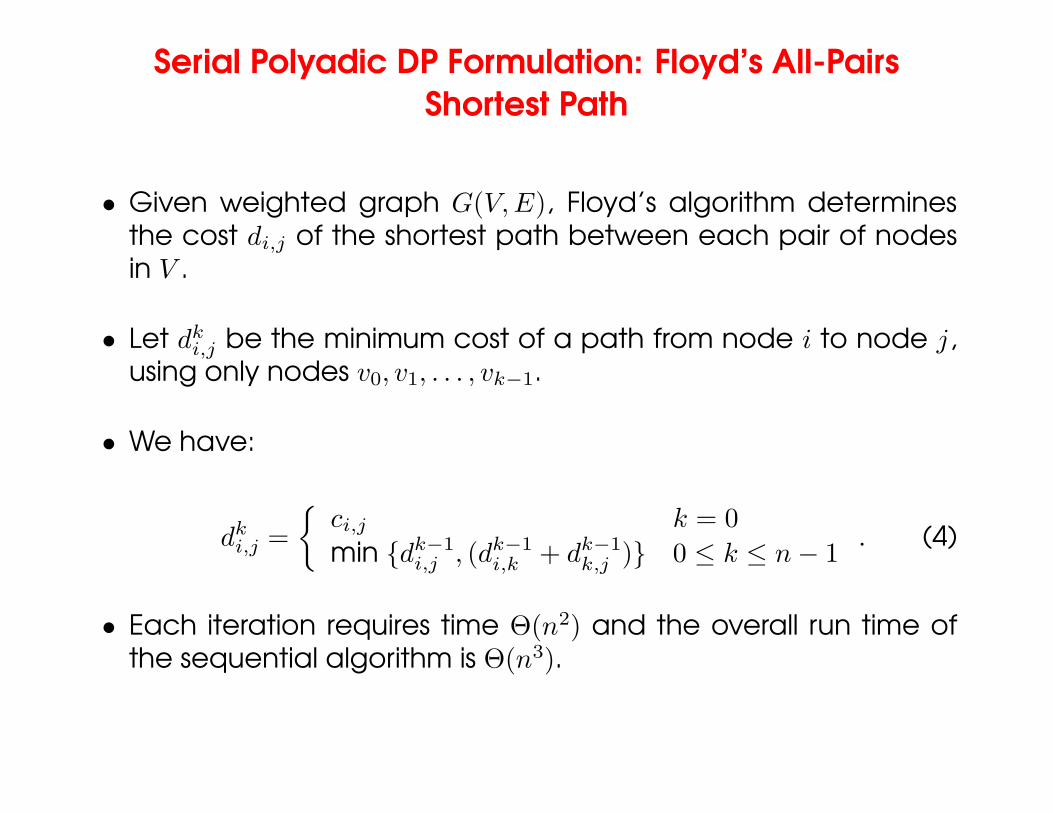
• Given weighted graph G(V, E), Floyd’s algorithm determinesthe cost di,j of the shortest path between each pair of nodesin V .

• Let dki,j be the minimum cost of a path from node i to node j,

using only nodes v0, v1, . . . , vk−1.

• We have:

dki,j =

{

ci,j k = 0

min {dk−1i,j , (dk−1

i,k + dk−1k,j )} 0 ≤ k ≤ n − 1

. (4)

• Each iteration requires time Θ(n2) and the overall run time ofthe sequential algorithm is Θ(n3).


Serial Polyadic DP Formulation: Floyd’s All-PairsShortest Path

• A PRAM formulation of this algorithm uses n2 processors in alogical 2D mesh. Processor Pi,j computes the value of dk

i,j fork = 1, 2, . . . , n in constant time.

• The parallel runtime is Θ(n) and it is cost-optimal.

• The algorithm can easily be adapted to practical architectures,as discussed in our treatment of Graph Algorithms.


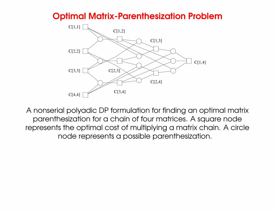
Nonserial Polyadic DP Formulation: OptimalMatrix-Parenthesization Problem

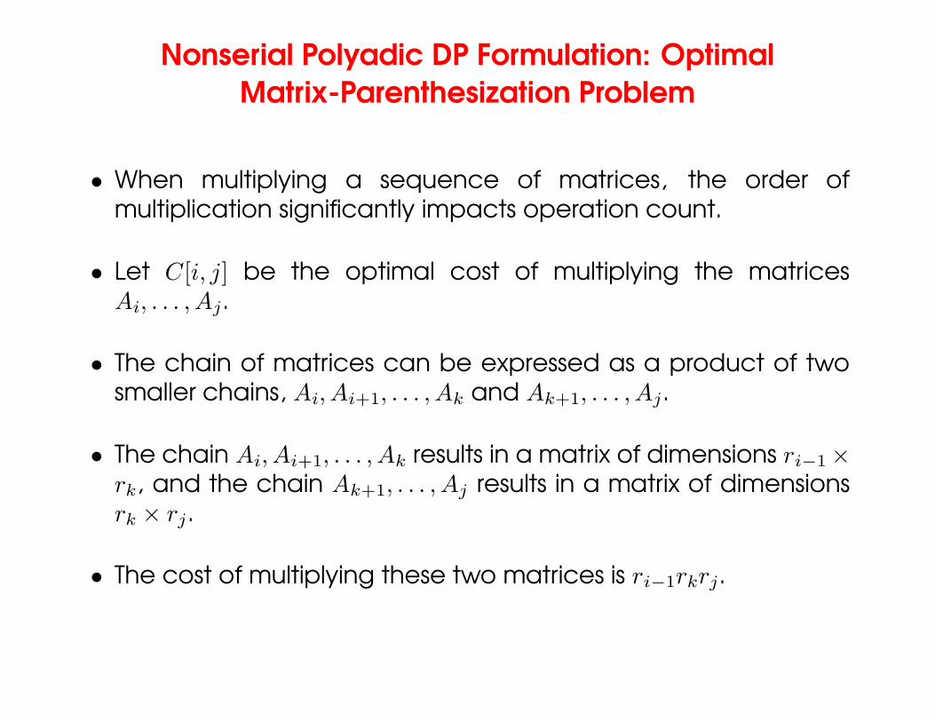
• When multiplying a sequence of matrices, the order ofmultiplication significantly impacts operation count.

• Let C[i, j] be the optimal cost of multiplying the matricesAi, . . . , Aj.

• The chain of matrices can be expressed as a product of twosmaller chains, Ai, Ai+1, . . . , Ak and Ak+1, . . . , Aj.

• The chain Ai, Ai+1, . . . , Ak results in a matrix of dimensions ri−1 ×rk, and the chain Ak+1, . . . , Aj results in a matrix of dimensionsrk × rj.

• The cost of multiplying these two matrices is ri−1rkrj.


Optimal Matrix-Parenthesization Problem

• We have:

C[i, j] =

{

mini≤k<j

{C[i, k] + C[k + 1, j] + ri−1rkrj} 1 ≤ i < j ≤ n

0 j = i, 0 < i ≤ n(5)



C[4,4]

C[3,3]

C[2,2]

C[1,1]C[1,2]

C[2,3]

C[3,4]

C[2,4]

C[1,3]

C[1,4]

A nonserial polyadic DP formulation for finding an optimal matrixparenthesization for a chain of four matrices. A square node

represents the optimal cost of multiplying a matrix chain. A circlenode represents a possible parenthesization.



• The goal of finding C[1, n] is accomplished in a bottom-upfashion.

• Visualize this by thinking of filling in the C table diagonally.Entries in diagonal l corresponds to the cost of multiplyingmatrix chains of length l + 1.

• The value of C[i, j] is computed as min{C[i, k] + C[k + 1, j] +ri−1rkrj}, where k can take values from i to j − 1.

• Computing C[i, j] requires that we evaluate (j − i) terms andselect their minimum.

• The computation of each term takes time tc, and thecomputation of C[i, j] takes time (j−i)tc. Each entry in diagonall can be computed in time ltc.



• The algorithm computes (n− 1) chains of length two. This takestime (n − 1)tc; computing (n − 2) chains of length three takestime (n − 2)2tc. In the final step, the algorithm computes onechain of length n in time (n − 1)tc.

• It follows that the serial time is Θ(n3).



Diagonal 1

Diagonal 2

Diagonal 7

Diagonal 6

Diagonal 0

(1,8)

(2,8)

(3,8)

(4,8)

(5,8)

(8,8)

(1,7)

(2,7)

(3,7)

(4,7)

(5,7)

(6,6)

(5,6)

(4,6)

(3,6)

(2,6)

(1,6)

(2,5)

(3,5)

(4,5)

(5,5)

(4,4)

(3,4)

(2,4)

(1,4)(1,3)

(2,3)(2,2)

(3,3)

(1,5)

(7,8)(7,7)

(6,7) (6,8)

(1,1) (1,2)

PSfrag replacements

P0 P1 P2 P3 P4 P5 P6 P7

The diagonal order of computation for the optimalmatrix-parenthesization problem.


Parallel Optimal Matrix-Parenthesization Problem

• Consider a logical ring of processors. In step l, each processorcomputes a single element belonging to the lth diagonal.

• On computing the assigned value of the element in table C,each processor sends its value to all other processors using anall-to-all broadcast.

• The next value can then be computed locally.

• The total time required to compute the entries along diagonall is ltc + ts log n + tw(n − 1).

• The corresponding parallel time is given by:

TP =n−1∑

l=1

(ltc + ts log n + tw(n − 1)),

=(n − 1)(n)

2tc + ts(n − 1) log n + tw(n − 1)2.


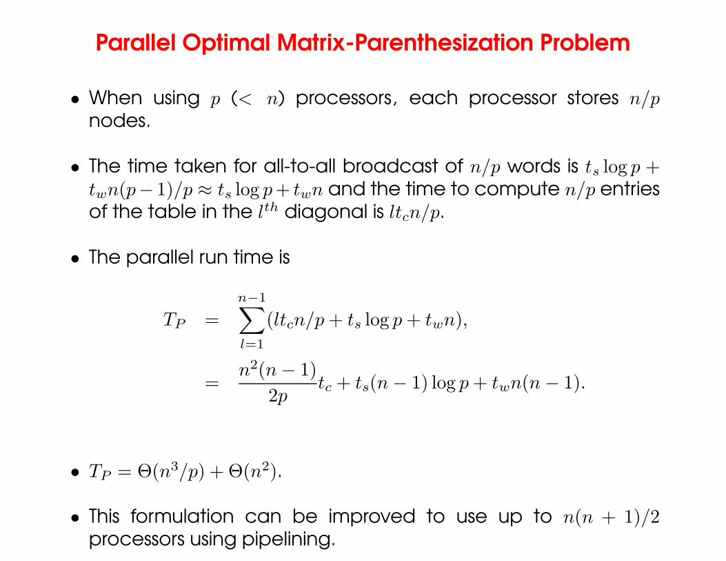
Parallel Optimal Matrix-Parenthesization Problem

• When using p (< n) processors, each processor stores n/pnodes.

• The time taken for all-to-all broadcast of n/p words is ts log p +twn(p− 1)/p ≈ ts log p+ twn and the time to compute n/p entriesof the table in the lth diagonal is ltcn/p.

• The parallel run time is

TP =

n−1∑

l=1

(ltcn/p + ts log p + twn),

=n2(n − 1)

2ptc + ts(n − 1) log p + twn(n − 1).

• TP = Θ(n3/p) + Θ(n2).

• This formulation can be improved to use up to n(n + 1)/2processors using pipelining.


Discussion of Parallel Dynamic ProgrammingAlgorithms

• By representing computation as a graph, we identify threesources of parallelism: parallelism within nodes, parallelismacross nodes at a level, and pipelining nodes across multiplelevels. The first two are available in serial formulations and thethird one in non-serial formulations.

• Data locality is critical for performance. Different DPformulations, by the very nature of the problem instance, havedifferent degrees of locality.


dynamic programming - university of minnesota · dynamic programming the dependencies between...

Documents