dynamic program analysis and optimization under dynamorio
TRANSCRIPT

THE UNIVERSITY OF MANCHESTER
Dynamic Program Analysis andOptimization under DynamoRIO
A THESIS
SUBMITTED TO THE UNIVERSITY OF MANCHESTER
FOR THE DEGREE OF
MASTER OFPHILOSOPHY (MPHIL )
IN THE FACULTY OF ENGINEERING AND PHYSICAL SCIENCES
Author:
Naweiluo ZHOU
Supervisors:
Prof. John GURD
Prof. Alasdair
RAWSTHORNE
School of Computer Science
2014

Contents
Abstract 10
Declaration 12
Copyright 14
Acknowledgements 16
Glossary 17
1 Introduction 22
1.1 Contribution . . . . . . . . . . . . . . . . . . . . . . . . . . . . . . . 24
1.2 Thesis Structure . . . . . . . . . . . . . . . . . . . . . . . . . . . . . 25
2 Background 27
2.1 Introduction . . . . . . . . . . . . . . . . . . . . . . . . . . . . . . . 27
2.2 Terminology . . . . . . . . . . . . . . . . . . . . . . . . . . . . . . . 28
2.3 Profiling Techniques . . . . . . . . . . . . . . . . . . . . . . . . . . 28
2.4 Data Flow and Control Flow Analysis . . . . . . . . . . . . . . . . . 29
2.5 Optimization Techniques . . . . . . . . . . . . . . . . . . . . . . . . 31
2.5.1 Introduction . . . . . . . . . . . . . . . . . . . . . . . . . . . 31
2.5.2 Software Prediction . . . . . . . . . . . . . . . . . . . . . . . 31
2.5.3 Optimization Algorithms in Software . . . . . . . . . . . . . 32
2.5.4 Hardware Prediction . . . . . . . . . . . . . . . . . . . . . . 34
2.5.5 Code Reuse in Hardware . . . . . . . . . . . . . . . . . . . . 35
2.6 Static Optimizers . . . . . . . . . . . . . . . . . . . . . . . . . . . . 36
2.6.1 Introduction . . . . . . . . . . . . . . . . . . . . . . . . . . . 36
2.6.2 MAO . . . . . . . . . . . . . . . . . . . . . . . . . . . . . . 37
2.6.3 Superoptimizer . . . . . . . . . . . . . . . . . . . . . . . . . 38
3

4 CONTENTS
2.6.4 Peephole Optimizer . . . . . . . . . . . . . . . . . . . . . . . 39
2.6.5 Summary . . . . . . . . . . . . . . . . . . . . . . . . . . . . 40
2.7 Dynamic Optimizer . . . . . . . . . . . . . . . . . . . . . . . . . . . 41
2.7.1 Introduction . . . . . . . . . . . . . . . . . . . . . . . . . . . 41
2.7.2 Dynamo . . . . . . . . . . . . . . . . . . . . . . . . . . . . . 43
2.7.3 DynamoRIO . . . . . . . . . . . . . . . . . . . . . . . . . . 44
2.7.4 Mojo . . . . . . . . . . . . . . . . . . . . . . . . . . . . . . 48
2.7.5 Wiggins/Redstone . . . . . . . . . . . . . . . . . . . . . . . 49
2.7.6 Java Virtual Machine and JIT compiler . . . . . . . . . . . . 49
2.7.7 Pin and its JIT compiler . . . . . . . . . . . . . . . . . . . . 51
2.7.8 HDTrans . . . . . . . . . . . . . . . . . . . . . . . . . . . . 52
2.7.9 Summary . . . . . . . . . . . . . . . . . . . . . . . . . . . . 55
2.8 Chapter Summary . . . . . . . . . . . . . . . . . . . . . . . . . . . . 56
3 Dynamic Code Analysis and Optimization 59
3.1 Introduction . . . . . . . . . . . . . . . . . . . . . . . . . . . . . . . 59
3.2 Methodology . . . . . . . . . . . . . . . . . . . . . . . . . . . . . . 59
3.2.1 Evaluation Test Case: SPEC CPU2006 . . . . . . . . . . . . 60
3.2.2 Configuration . . . . . . . . . . . . . . . . . . . . . . . . . . 62
3.3 Base Performance of DynamoRIO . . . . . . . . . . . . . . . . . . . 62
3.4 Experiment 1—Removal of Redundant Instructions . . . . . .. . . . 66
3.5 Experiment 2—Strength Reduction . . . . . . . . . . . . . . . . . . .70
3.6 Experiment 3—Instruction Alignment . . . . . . . . . . . . . . . .. 72
3.6.1 Analysis of Rationales fornopOptimization . . . . . . . . . . 77
3.6.2 Memory References Simulator . . . . . . . . . . . . . . . . . 78
3.6.3 Branch Target Prediction Simulator . . . . . . . . . . . . . . 79
3.6.4 Cache Simulator . . . . . . . . . . . . . . . . . . . . . . . . 81
3.7 Experiment 4—Persistent Code . . . . . . . . . . . . . . . . . . . . . 83
3.8 Experiment 5—Glacial Address Propagation . . . . . . . . . . .. . . 84
3.8.1 Constant Addresses Analysis . . . . . . . . . . . . . . . . . . 85
3.8.2 Instrumentation Optimization . . . . . . . . . . . . . . . . . 90
3.9 Chapter Summary . . . . . . . . . . . . . . . . . . . . . . . . . . . . 92
4 Conclusion and Discussion 95
4.1 Introduction . . . . . . . . . . . . . . . . . . . . . . . . . . . . . . . 95
4.2 Conclusion and Discussion . . . . . . . . . . . . . . . . . . . . . . . 95

CONTENTS 5
4.3 Future Work . . . . . . . . . . . . . . . . . . . . . . . . . . . . . . . 97
4.3.1 Integration of Static and Dynamic Optimization . . . . .. . . 97
4.3.2 Glacial Addresses Optimization and Multiple Threading . . . 97
4.3.3 Memory Management . . . . . . . . . . . . . . . . . . . . . 98
4.3.4 Possible Application Analysis . . . . . . . . . . . . . . . . . 99
4.3.5 Energy Consumption Management . . . . . . . . . . . . . . . 99
Bibliography 101

List of Figures
1.1 The working layer of virtual systems . . . . . . . . . . . . . . . . .. 23
2.1 Value prediction . . . . . . . . . . . . . . . . . . . . . . . . . . . . . 34
2.2 Instruction reuse in a typical processor . . . . . . . . . . . . .. . . . 35
2.3 Structure of the peephole optimizer . . . . . . . . . . . . . . . . .. . 40
2.4 How Dynamo works . . . . . . . . . . . . . . . . . . . . . . . . . . 44
2.5 Basic infrastructure of DynamoRIO . . . . . . . . . . . . . . . . . .46
2.6 The deployment of DynamoRIO and its client . . . . . . . . . . . .. 47
2.7 Basic structure of Mojo . . . . . . . . . . . . . . . . . . . . . . . . 48
2.8 How JVM works . . . . . . . . . . . . . . . . . . . . . . . . . . . . 50
2.9 The basic architecture of Pin . . . . . . . . . . . . . . . . . . . . . . 52
2.10 Benchmarks performance of Pin and DynamoRIO . . . . . . . . .. . 53
2.11 An example of source instructions . . . . . . . . . . . . . . . . . .. 54
2.12 An example of translated instructions . . . . . . . . . . . . . .. . . 54
3.1 Simple benchmark performance for all workloads . . . . . . .. . . . 65
3.2 Simple benchmark performance of test and reference workload . . . . 66
3.3 Redundanttestinstruction . . . . . . . . . . . . . . . . . . . . . . . 67
3.4 DynamoRIO routine for instrumenting in a trace. . . . . . . .. . . . 69
3.5 Benchmark performance on thetestremoverandempty . . . . . . . 70
3.6 Equivalent instructions . . . . . . . . . . . . . . . . . . . . . . . . . 71
3.7 Benchmark performance foradd2leaclient andempty client . . . . . 72
3.8 Benchmark performance fluctuation when removingnop . . . . . . . 74
3.9 A trace example . . . . . . . . . . . . . . . . . . . . . . . . . . . . . 75
3.10 Performance fluctuation of each trace . . . . . . . . . . . . . . .. . 76
3.11 A DynamoRIO function call for insertingnop . . . . . . . . . . . . . 77
3.12 The DynamoRIO calls to determine memory references . . .. . . . . 79
3.13 The DynamoRIO branch instrumentation function calls .. . . . . . . 80
6

LIST OF FIGURES 7
3.14 Thread initialisation and termination routines . . . . .. . . . . . . . 82
3.15 DynamoRIO calls to enable data to be saved in persistentcache . . . . 83
3.16 Persistent code performance comparison . . . . . . . . . . . .. . . . 84
3.17 The way for labelling stage levels . . . . . . . . . . . . . . . . . .. 87
3.18 Codes to obtain the register value under DynamoRIO . . . .. . . . . 88
3.19 Codes to obtain the execution frequency of each block . .. . . . . . 88
3.20 Stage information oflibquantum andmcf . . . . . . . . . . . . . . . 89
3.21 The DynamoRIO function to generate a client thread . . . .. . . . . 91
3.22 Multi-threading procedure . . . . . . . . . . . . . . . . . . . . . . .92
4.1 The infrastructure of the optimization system . . . . . . . .. . . . . 98

List of Tables
3.1 SPEC CPU2006 packages . . . . . . . . . . . . . . . . . . . . . . . 62
3.2 Default DynamoRIO client details . . . . . . . . . . . . . . . . . . .63
3.3a Time spent on each test workload benchmark . . . . . . . . . . .. . 67
3.3b Time spent on each train workload benchmark . . . . . . . . . .. . . 68
3.3c Time spent on each reference workload benchmark . . . . . .. . . . 69
3.4 Total number oftestinstructions detected and deleted . . . . . . . . . 70
3.5 Total number ofadd in the traces of benchmarks . . . . . . . . . . . . 72
3.6 Equivalent tonop instructions in DynamoRIO . . . . . . . . . . . . . 73
3.7 An example of indirect address candidates . . . . . . . . . . . .. . 85
3.8 An example of substitution instructions . . . . . . . . . . . . .. . . 86
3.9 Stage information oflibquantum andmcf . . . . . . . . . . . . . . . 89
3.10 Average glacial address number in each stage level . . . .. . . . . . 89
3.11 Sum of glacial addresses in each stage level of the program . . . . . . 90
3.12 A list of all the implemented clients . . . . . . . . . . . . . . . .. . 93
8


Abstract
A thesis submitted for the degree of Master of Philosophy
Title: Dynamic Program Analysis and Optimization under DynamoRIO
By Naweiluo Zhou, The University of Manchester, 5th February 2014
The thesis presents five experiments using DynamoRIO to analyse and optimize ma-
chine codes at runtime in various ways and observe the effectof each optimisation
using the SPEC CPU2006 benchmarks as test case codes.
Software often stays unchanged for periods measured in years, while new CPU
chips are introduced every 18 months or so. In addition, it isoften not realized how
modern CPU chips adjust their behaviour, and their performance, in response to dy-
namic conditions arising in the software that is running. Dynamic optimization is
carried out while a program runs. It calls on the knowledge ofruntime behaviour of
the program, which causes high runtime overhead.
Programs can show performance gain by applying removal of redundant instruc-
tions, strength reduction, instruction alignment and persistent code. Strength reduction
replaces expensive instructions with cheap counterparts.The code layout in the mem-
ory could affect the cache miss rate and the branch mis-prediction rate of the proces-
sor, which affect program performance. An optimized program could be recorded as
persistent cache, then loaded directly in the subsequent calls. One dynamic program
analysis method, glacial address propagation, is also presented. The values of glacial
indirect addresses change slowly, making each value act as aconstant address for a pe-
riod, thus enabling a cascade of optimizations. To accelerate information processing,
profile information is processed by multiple threads in parallel.
Therefore, programs can be made to run more quickly using a variety of optimiza-
tion carried out at runtime, aided by observation of controlflow, data flow, and memory
access patterns of programs. Future work could perform static optimization before dy-
namic optimization. The hardware power consumption will betaken into account.
10

Declaration
No portion of the work referred to in this thesis has been submitted in support of an
application for another degree or qualification of this or any other university or other
institute of learning.
12


Copyright
i The author of this thesis (including any appendices and/orschedules to this thesis)
owns certain copyright or related rights in it (the “Copyright”) and she has given
The University of Manchester certain rights to use such Copyright, including for
administrative purposes.
ii Copies of this thesis, either in full or in extracts and whether in hard or electronic
copy, may be madeonly in accordance with the Copyright, Designs and Patents
Act 1988 (as amended) and regulations issued under it or, where appropriate, in
accordance with licensing agreements which the Universityhas from time to time.
This page must form part of any such copies made.
iii The ownership of certain Copyright, patents, designs, trade marks and other intel-
lectual property (the “Intellectual Property”) and any reproductions of copyright
works in the thesis, for example graphs and tables (”Reproductions”), which may
be described in this thesis, may not be owned by the author andmay be owned by
third parties. Such Intellectual Property and Reproductions cannot and must not
be made available for use without the prior written permission of the owner of the
relevant Intellectual Property and/or Reproductions.
iv Further information on the conditions under which disclosure, publication and
commercialisation of this thesis, the Copyright and any Intellectual Property and/or
Reproductions described in it may take place is available inthe University IP Policy
(see http://documents.manchester.ac.uk/DocuInfo.aspx?DocID=487), in any rele-
vant Thesis restriction declarations deposited in the University Library, Them Uni-
versity Library’s regulations1 and in The University’s policy on Presentation of
Theses.
1 See http://www.manchester.ac.uk/library/aboutus/regulations
14


Acknowledgements
The two years spent in Manchester is one of my most joyful, peaceful periods in life.
I must express my appreciation to all the people who have helped me. I shall and will
remember all the kindness.
I would like to take this chance to especially thank my supervisor Prof. John Gurd.
He advised me on the experiments and support me to fix and complete the thesis. He
also offers great help on my future career.
I also would like to express my gratitude to my supervisor Prof. Alasdair Raw-
sthorne who leaded me to the research area in program analysis and optimization.
I have to express my gratitude to Dr. Barry Cheetham who has helped me for the
last two years. I would like to thank him for his constructiveadvice on my research as
well as my future career.
16

Glossary
Symbols | L
Symbols
Boolean Test
test if two instructions’ minterms of the Boolean argumentsmatch. 38
Constant propagation
analyse a variable whose value is a constant. 30
DynamoRIO basic block
a sequence of instructions ending with a control transfer instruction. 45
DynamoRIO trace
a piece of hot code constructed by modified NET algorithm. 32,45
DynamoRIO
a runtime code manipulation system. 44
Mojo fragment
a piece of code with additional control transfer instructions in Mojo. 48
Mojo path
consists of multiple basic blocks. 48
Probabilistic Test
test if the output results match the original program. 38
SPEC CPU2006
a benchmark suite. 60
address profile
memory addresses references. 29
17

18 Glossary
application thread
works in DynamoRIO’s code cache. 90
basic block cache
DynamoRIO’s code cache. 45
benchmark
a computer program that performs set operations. 61
binary translation
translate one type of executable to another. 41
client thread
run natively. 90
client
perform runtime code manipulation. 46
code cache
a part of memory space allocated by an optimizer. 28
context switch
DynamoRIO saves and restores the general-purpose registers, the condition codes
(eflags register) and any operating system dependent state.45
context
information of integer registers, flag registers, instruction pointers and the pro-
gram stacks. 36
control flow profile
information of program execution path. 29
dynamic optimization
performs optimization during program execution. 27
equivalence tests
test if two instructions perform the same function. 38
fragment
another expression of trace. 28

Glossary 19
glacial address propagation
label the indirect addresses with useful properties. 85
glacial variables
slowly change variables. 30
hot
the wordhot in this thesis means frequently-executed. 23
instrumentation
a technology for inserting extra codes into a program. 51
just-in-time compilation
compile a machine-independent program for a processor. 41
offline profiling
performed before the program executes. 29
online profiling
records the information during program execution. 29
path
another expression of trace. 28
profile
information of the distribution of call sites, parameter values, the execution times
of each basic block of the program,etc. 29
reference workload
simulate the function of the real application. 61
stage level
a stage level is a basic block labelled with useful properties. 86
stage
a set of basic blocks, a stage ends with a special control transfer instruction. 86
static optimization
optimizes the program during compile time. 27
test workload
a simple version of reference workload. 61
20 Glossary
trace cache
DynamoRIO’s code cache. 45
trace
a trace in a dynamic optimizer is a piece of code which is frequently executed.
28
traditional basic block
a sequence of instructions with a single entry and single exit. 36
traditional trace
a large sequence of instructions. 36
train workload
takes more time to finish than the test workload. 61
transparent optimization
take binary executable and re-optimize it. 41
value profile
information of the specific values. 29
L
LSD
Loop Stream Detector. 38

Chapter 1Introduction
21

Chapter 1
Introduction
Program optimization is ubiquitous, as it improves programperformance though either
reducing the program size or accelerating program execution. Programs run faster on
newer generation CPU silicon. Production software, though, often stays unchanged for
periods measured in years, while new CPU chips are introduced every 18 months or
so. In addition, it is often not realized how modern CPU chipsadjust their behaviour,
and their performance, in response to dynamic conditions arising in the program that is
running. For example, a modern CPU chip will adjust the orderof instructions issued,
the memory references it carries out, and the order in which it fetches instructions
depending on the exact pattern of execution in recent history, since it uses its own
observation of that history to attempt to run future instructions more speedily.
A compiler takes the high-level input source program and outputs the equivalent
but low-level sequences of instructions which are usually machine codes. Compilation
mainly includes five phases [3]: lexical analysis, syntax analysis, intermediate code
generation, code optimization and code generation. Code optimization carried out
during compile time is called static optimization (detailsare given in Section 2.6) and
no online information is available. In contrast, Dynamic optimization (details are given
in Section 2.7) is performed as the program runs, enabling itto call on knowledge about
the runtime behaviour of the program.
Modern software applications heavily make use of shared libraries, dynamic class
loading, virtual functions, plugins, dynamically-generated code, and other dynamic
mechanisms. Optimization decisions really need to be deferred until all the relevant in-
formation is available. Dynamic code optimization shows its advantage over static op-
timization in four respects (the detail will be covered in Chapter 2). First and foremost,
22

23
it makes the program work more efficiently compared with static optimization. Sec-
ondly, dynamic optimization makes use of prediction of runtime program behaviour, as
runtime profile information is available. Thirdly, modern software [7] is being shipped
as a collection of DLLs (Dynamically Linked Libraries), making it difficult for a static
compiler to analyse the whole program [11]. Finally, dynamic code manipulation sys-
tems can solve hardware compatibility problems for cross-platform application-level
virtualization (e.g.Apple Rosetta1).
However, dynamic optimization suffers from its own problems. The most signif-
icant disadvantage is that it slows down program execution due to collection of the
runtime information (e.g. hot2 region analysis, memory usage analysis). A number of
runtime systems, such as Dynamo [15], DynamoRIO [13] and Wiggins/Redstone [18],
have been developed in order to perform runtime code optimization and also confine
overhead to a low level.
The most well-known and widely-used code manipulation system is the Java Vir-
tual Machine.3 Figure 1.1 gives a view of where these runtime code manipulation
systems (known as virtual systems) reside in a compilation and execution procedure.
The left of the figure shows the system without the virtual system. The right of the
figure shows the system with the virtual system. The details of all these systems are
presented in Chapter 2.
Figure 1.1: The working layer of virtual systems. The left side is the traditional view;the right side is the virtual system view
The thesis focuses on dynamic program analysis and optimization, as dynamic op-
timization is able to adapt its optimization approaches to match the runtime behaviour
1 Apple Rosetta, http://www.apple.com/asia/rosetta/, accessed on 30/05/2012.2 The wordhot in this thesis means frequently-executed.3 JVM, available from http://docs.oracle.com/javase/specs/jvms/se7/html/jvms-1.html, accessed on
17/04/2012.
24 CHAPTER 1. INTRODUCTION
of the program. DynamoRIO, an open-source software, is the runtime code manipu-
lation system employed in this thesis to perform program analysis and optimization.
Firstly, its input is the binary stream, making the platformlanguage-independent. Plus
in some cases, source codes of the program are not available,hence code optimization
cannot rely on the compiler. Secondly, DyanmoRIO is flexible, as it is able to perform
optimizations which tailor the program to the actual processor it is running on. In other
words, DynamoRIO can efficiently make use of underlying hardware mechanisms.
Thirdly, DynamoRIO provides a good user interface for manipulating the runtime pro-
gram. Additionally, DynamoRIO can tackle the machine code directly, such as branch
inlining and instruction replacement,etc. The compiler usually performs optimization
on intermediate representation codes which is generally considered to be easier than
optimization on machine code. However, it is an open question whether recompila-
tion in order to perform the optimization is more time-consuming or performing the
optimization on the machine code directly causes more overhead.
1.1 Contribution
This thesis investigates runtime code analysis and optimization methodologies. Strength
reduction (Section 3.5) has been applied in DynamoRIO in a previous publication [44],
but this thesis expands and presents the method in detail. Three methods in this thesis
are modifications of existing work. This includes redundantinstruction detection (Sec-
tion 3.4), instruction alignment optimization (Section 3.6) and glacial address propa-
gation (Section 3.8). There are some publications that showsimilar research on redun-
dant instruction detection as well as instruction alignment, but none of them apply the
above schemes in the runtime environment under DynamoRIO asin this thesis. Glacial
address propagation is a modification of glacial variable analysis [4]. This algorithm
aims to discover the potential slowly changing addresses during program execution.
As glacial indirect addresses are changed slowly and could be considered to be a con-
stant address for a period, these indirect addresses are candidates for code replacement
aiming for code optimization.
The experimental results in the thesis demonstrate that some benchmarks gain per-
formance at a single digit percentage level through dynamicprogram optimization. A
dynamic program analysis method, glacial address propagation, shows the potential
candidates in a program which may enable a cascade of code optimization.

1.2. THESIS STRUCTURE 25
1.2 Thesis Structure
The thesis investigates and explores runtime program analysis and optimization method-
ologies. The runtime code manipulation system, DynamoRIO,which supports code
transformation on any part of programs, is exploited as a development tool to inves-
tigate the design space for optimizers between the current state of the art in static
and dynamic languages. DynamoRIO provides interfaces (details are given in Sec-
tion 2.7.3) which enable development of program analysers to observe and potentially
manipulate every single instruction prior to its execution. Although there is runtime
profile overhead, the overall execution time of the application can be decreased in cer-
tain cases.
This thesis first describes background techniques and technologies in Chapter 2.
Then it presents the five experiments on program analysis andoptimization in Chap-
ter 3. The experiments incorporate redundant instruction detection and removing (Sec-
tion 3.4), strength reduction optimization (Section 3.5),instruction alignment (Sec-
tion 3.6), persistent cache (Section 3.7) and glacial address propagation (Section 3.8).
Discussion of the experimental results and potential future work are presented in Chap-
ter 4.

Chapter 2Background
26

Chapter 2
Background
2.1 Introduction
The performance of a program is essentially determined by its size and running time.
Program optimization is ubiquitous, as it improves programperformance though ei-
ther reducing the program size or accelerating program execution. Static optimization,
which is employed in almost all compilers, optimizes the program during compile time
to produce better performance of codes.Dynamic optimization, which is found for ex-
ample in a Java Just-In-Time compiler, performs optimization during program execu-
tion, enabling the discovery of runtime information which is not available at compile
time. Feeding back such information could enable the compiler to make better de-
cisions in its optimization algorithms, but an alternativeway of searching for code
optimization is from dynamic optimizers. Such an optimizerdoes not perform com-
plex lexical analysis and syntax analysis, as the compiler does [3], rather it performs
optimization on the machine code (e.g.assembly level or binary level).
This chapter briefly reviews the background techniques and technologies for code
analysis and optimization to help better understand Chapter 3. The chapter is organised
as follows. It first reviews program analysis methods, as program analysis provides
necessary information for the choice of program optimizations. Profiling techniques
(Section 2.3) and data flow/control flow analysis (Section 2.4) are two program anal-
ysis techniques. Section 2.5 gives optimization techniques. These are the algorithms
contributing to an optimizer, a compiler’s basic working procedure or the basic code
optimization algorithms guiding complex algorithm design. The two next sections
(Section 2.6 and Section 2.7) review optimization technologies in the working proce-
dure of some optimizers. Section 2.6 reviews three static optimizers. In Section 2.7
27

28 CHAPTER 2. BACKGROUND
seven well-known dynamic optimizers are reviewed to help gain a better understanding
of how a runtime system works on code optimization.
2.2 Terminology
This section explains some critical terminology used in this chapter and the rest of the
thesis.
Dynamic optimizers share a common and important characteristic, that is building
traces. Atraceis a piece of code which is frequently executed. This piece ofcode may
contain some repeated codes (due to code inlining) occupying a continuous space in
the memory/cache, thus enabling faster code execution in the processor. As building a
trace needs runtime program information, a traditional compiler is unable to construct a
trace. The term trace is also expressed aspathor fragmentin some optimizers, however
they all refer to a sequence of instructions with a large amount of code reuse, although
the details may differ slightly. To build traces, prediction algorithms are required in
order to know which branch will be executed next. A good prediction algorithm could
significantly improve program performance. A dynamic optimizer and the underlying
hardware could both provide branch prediction. Section 2.5and Section 2.5.4 will
explain the difference between the two.
Based on its static characteristics, a compiler can offer various optimization algo-
rithms to the whole program. An example is the well-known algorithm known as loop
inlining. A dynamic optimizer can provide the same optimization algorithms as a com-
piler, however, as a dynamic optimizer has more runtime program information, it can
also use this to choose to only apply optimization algorithms to certain regions of a
program and skip others. This can avoid time being wasted on optimizing infrequently
executed instructions. In dynamic optimizers, optimized traces are typically placed in
a code cache. Acode cacheis a part of memory space allocated by an optimizer. Code
that executes from the code cache is like executing natively. In different dynamic opti-
mizers, the code cache is also called by different names, such as fragment cache, trace
cache, path cache and basic block cache.
2.3 Profiling Techniques
Program profiling collects the specified offline or online information of the program.
This information can be called by a programmer or another program to influence the

2.4. DATA FLOW AND CONTROL FLOW ANALYSIS 29
optimization strategy to make the program run faster [34]. The profile information
refers to the distribution of call sites, parameter values,the execution times of each
basic block of the program and so on. As modern CPUs are becoming more and more
complex [34], programmers have little knowledge to understand how their program
interacts with such complicated hardware. Program profiling is thus an important step
for program optimization.
Offline profilingis performed before the program executes. The statistics are gath-
ered when the program runs one or more times. In contrast, anonline profiling tool
records the information during program execution. Hardware can provide profiling
information directly. For example, Intel processors have hardware performance coun-
ters [1] which can gather detailed profile information such as cycles executed, data
cache misses, data cache lines allocated, branches mis-prediction, instruction costet
al. Program Counter Sampling [13] can be exploited to analyse where time is spent in
execution of a program.
Different types of optimization require different types ofprofile information. Three
types of profile [23] are often used, namely control flow profile, value profile and ad-
dress profile.Control flow profilerecords the program execution path, which can help
determine the execution frequencies of certain paths of a program. Value profileob-
tains information about the specific values of operands as well as their frequency of oc-
currence.Address profilecollects the memory addresses references, which can be used
to apply data layout and placement transformations for improving the performance of
the memory hierarchy.
Profile-guided optimization [36] is widely applied in the compiler and the opti-
mizer as discussed in Section 2.7. Data flow and control flow analysis, described in the
next section, are also ways to collect profile information.
2.4 Data Flow and Control Flow Analysis
Data flow and control flow analysis help to profile useful information for program op-
timization; these are usually performed on programs written in a high-level language.
Some optimizations can be achieved by knowing various pieces of information ob-
tained from inspecting the whole program; for instance, expression analysis for global
redundancy elimination. Live variable analysis is helpfulfor global register allocation,
dead variable elimination and uninitialized variable detection. Some statements may
30 CHAPTER 2. BACKGROUND
cause redundant re-computation of values. If such re-computation can be safely elim-
inated, the program may execute faster. It is also helpful todivide the program into
blocks and analyse the control transfer information among the blocks. This helps the
programmer to understand the program execution direction.One way of doing con-
trol flow analysis [46] is to note down the starting address ofeach block. The above
analyses are known as data flow analysis and control flow analysis.
Constant propagation[43] is a well-known global data flow analysis whose goal
is to discover a value that is constant during all its possible executions and propagate
the constant value as far as possible through the program. The constant propagation
technique serves several purposes for program optimization:
• Codes that are never executed can be deleted, for instance unreachable expres-
sions or branches, which simplifies the program.
• It can reduce the number of memory accesses. Variables whosevalues stay con-
stant during their execution period can be replaced by constants.
• It avoids unnecessary computation by replacing an expression which holds a set
result (a constant) every time it is used.
While a program executes, some data values change sufficiently slowly that they can
be identified as “glacial variables”. Such glacial variables can be worthy of generating
special-case code in which each value is treated as a constant for a period, thus enabling
a cascade of optimizations [4]. These glacial variables arediscovered through online
data flow and control flow analysis. Such analysis is a modification of constant prop-
agation analysis. It is composed of two parts. The first part is called global recursion
level analysis, which labels the stage level of the loop and identifies their execution
frequency. The outer loop is Stage 0 and inner loop is Stage n (n=1,2,3...). The second
part is glacial variable propagation, which measures how frequently the value of the
variable changes. The stage level (e.g.Stage 0, Stage 1...) is captured for the variable
modified in a loop as well as the final value of variable exitingthe loop. This is an
interesting approach to optimization which is investigated further in Section 3.8.
2.5. OPTIMIZATION TECHNIQUES 31
2.5 Optimization Techniques
2.5.1 Introduction
The rationales [3] behind code optimization consist of detecting patterns in the pro-
gram and replacing the patterns by more efficient constructs. The replacement strate-
gies can be machine-dependent or machine-independent. This thesis mainly takes ac-
count of machine-independent strategies. This section focuses on optimization tech-
niques that either are contributing to optimizers’ basic working procedures or as the
basic concepts to guide more complex user-designed optimization algorithms to im-
plement in optimizers. Software and hardware optimizationmethods are reviewed.
A variety of software and hardware prediction mechanisms (Section 2.5.2 and Sec-
tion 2.5.4) are surveyed, as prediction mechanisms play an important role for code
optimization. Section 2.5.3 and Section 2.5.5 discuss optimization algorithms on a
program and underlying hardware mechanisms for code reuse to speed up program
execution.
Optimization techniques reviewed in this section are the common and basic opti-
mization strategies. Section 2.6 and Section 2.7 focus on program optimizers work.
2.5.2 Software Prediction
Dynamic optimizers usually incorporate software prediction algorithms to improve
program performance. Prediction algorithms provide useful information for building
traces as well as selecting appropriate regions for code optimization.
Dynamo (see Section 2.7.2), which is a dynamic optimizer, exploits a simple scheme
for trace prediction: Most Recently Executed Tail (MRET). Dynamo starts a counter
associated with a trace head. A backward taken branch (likely to be a loop head) or
an exit branch from a previously hot trace is a candidate for atrace head. A counter
keeps recording until it exceeds a threshold. When the counter reaches a threshold, the
trace head is recorded. This simple scheme only records the trace head, as it is likely
that, when an instruction or basic block becomes hot, its following instructions are also
hot. Therefore, instead of profiling the rest of branch instructions, Dynamo predicts
the tail of instructions following the hot trace head. This saves the storage space for the
counter, as counters are only maintained for the potential loop head. MRET is called
Next Executing Tail (NET) in later publications [19]. DynamoRIO, another dynamic
optimizer (Section 2.7.3), utilises NET with a small changeto control the overhead. In

32 CHAPTER 2. BACKGROUND
NET, it considers all backward branches as a trace head, DynamoRIO ignores back-
ward indirect branches so that the number of trace heads is reduced. More trace heads
may lead to larger numbers of tiny traces, which is undesirable.
Dynamic optimizers implement trace-based selection algorithms for hot-spot de-
tection and construction. However, trace-selection algorithms suffer from two prob-
lems: trace separation and excessive code duplication [24]. Trace separation occurs
when associated paths1 are selected to be separate traces and these traces may be
placed far apart from each other. This means there is always adelay when calling
or identifying the next execution trace as well as the delay for control jumps between
traces. The second problem stems from common parts of related traces; isolating these
traces leads to code duplication. Davidet al. [24] give two prediction algorithms to
solve the above problems: region-selection algorithms which are Last-Executed Itera-
tion algorithm (LEI) and trace-combination algorithm.
LEI is similar to NET but surpasses NET when identifying cyclic paths2 of exe-
cution. As in NET, LEI first searches whether the target branch is in the code cache.
Working from the code cache is more efficient than working by emulation (more de-
tails are given in Section 2.7.3). If the target branch is in the code cache, control is
transferred to the code cache, otherwise it is retrieved from the branch historic buffer.
A hashtable is provided to make the retrieval more efficient.Only a cyclic path is se-
lected from the historic buffer. The branches in the buffer are removed when selected
to form a trace. Trace-combination is an extension of trace selection, it simply rejoins
certain frequently-executed traces to prevent excessive code duplication. This oper-
ation requires space for caching traces before combinationwhich causes a memory
overhead even if only a compact representation of each traceis stored.
2.5.3 Optimization Algorithms in Software
Optimization Methods for Array References
Compilers apply two approaches [3] that permit array references as operands:
• The reference to the array will not change until the code generation phase. It is
in the code generation phase that the offset of an array and its base address are
generated. And then an indexing operation is performed.
1 Path in Section 2.5.2 is not the terminology that is used in dynamic optimizers, but the literalmeaning.
2 A cyclic pathis simply a path that ends with a branch to its beginning.

2.5. OPTIMIZATION TECHNIQUES 33
• The array references are expanded into three-address statements that do the off-
set calculation. The three-address statement is typicallyof the general form
A:=B op C. Where A, B and C can be a programmer-defined name (a constant
or compiler-generated temporary name) and op stands for anyoperator (such
as an arithmetic operator). This approach is widely appliedfor optimization of
array reference in loops to improve locality of reference inmemory.E.g, assum-
ing a two-dimensional 10x20 array A, A[i,j] is in locationaddr(A)+20(i-1)+j-1
which is equal to(addr(A)-21)+20i+j. The machine code to reference A[i,j] will
compute20i+j in an index register. The three-address statement to evaluate the
element of an A[i,j] into a temporary T would look like this:
code to evaluate i into temporary T1
T2:=20*T1
code to evaluate j into temporary T3
T4:=T2+T3
T:=(addr(A)-21)+[T4]
Usually there is a base register for storing the starting address of the array, so the
compiler can determine the starting addresses at the beginning of the program.
The offset is calculated either by the final compilation phase (code generation
phase) or by the loader.
The details of optimization for array references are beyondthe scope of the thesis;
more information can be found in [3].
Inner Loop
It is generally accepted that most of the running time is spent in a small part of a
program: for example, 90% of the time is used by 10% of the program. So the “inner
loop”, the most-frequently executed part, is the first target for code optimization.
The running time of a program may decrease when the length of an inner loop is
shortened, even when the number of instructions outside theloop increases. Induction
variable elimination can reduce the number of arguments in aloop by merging vari-
ables. Choosing cheaper operations, for instance substituting multiplications by addi-
tions, can improve the performance. This optimization is called strength reduction. On
top of that, loop unrolling [3] and loop jamming [3] can sometimes be utilized to make
the loop execute more quickly.
34 CHAPTER 2. BACKGROUND
2.5.4 Hardware Prediction
Branch Prediction
Hardware provides schemes [14, 33] to perform branch prediction. The simplest strat-
egy is the so-called one-bit branch prediction buffer [29].The buffer is a small memory
indexed by the least significant bits of the branch instruction address. It incorporates
a bit specifying whether the branch is recently taken or not:1 is for taken, 0 is for
not-taken. The bit will be inverted if the branch predictionturns out to be wrong. For
example, bit=1 indicates that the associated branch is predicted to be taken when next
executed. A slightly more complicated but more reliable branch prediction uses two
bits for branch prediction. The value is between 0 and 3. Prediction must fail twice
in succession before it is changed. Bits are incremented when branch is predicted as
taken otherwise stays as 0 or decremented. Only 2 and 3 indicate that branch will be
taken in the next round execution. Compared with 1-bit prediction, two-bit prediction
can avoid the constant mis-prediction when a branch is takenand not-taken alternately.
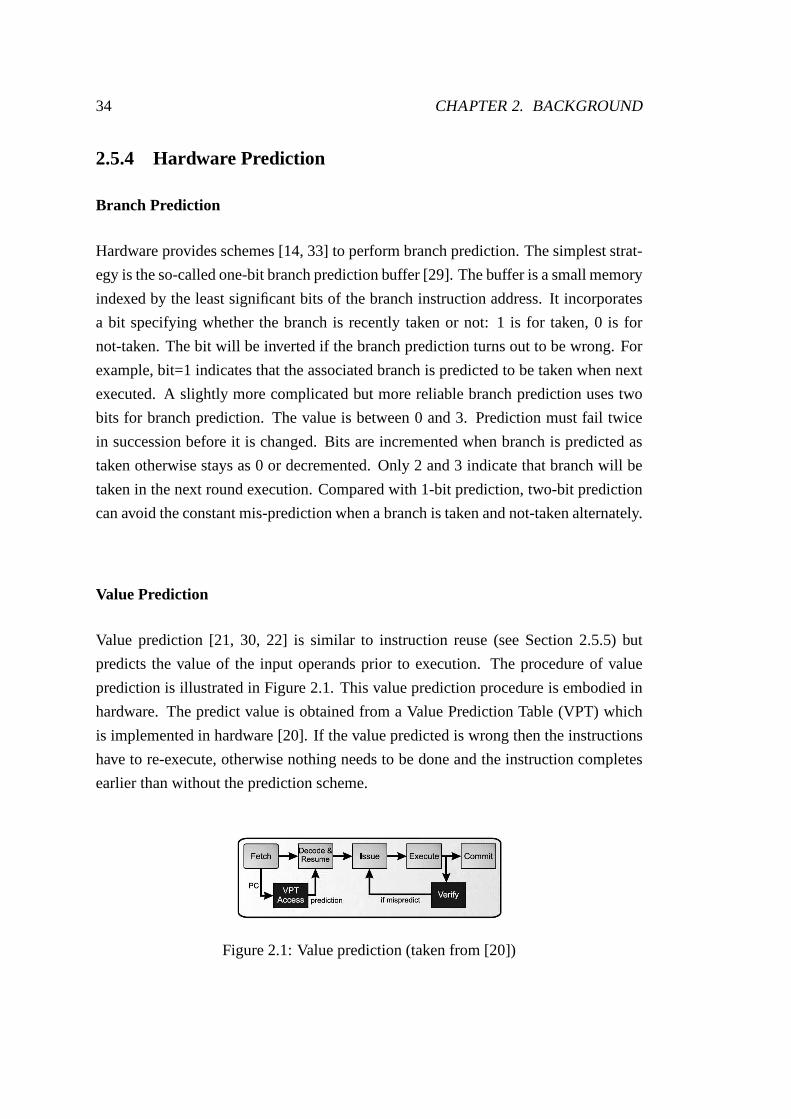
Value Prediction
Value prediction [21, 30, 22] is similar to instruction reuse (see Section 2.5.5) but
predicts the value of the input operands prior to execution.The procedure of value
prediction is illustrated in Figure 2.1. This value prediction procedure is embodied in
hardware. The predict value is obtained from a Value Prediction Table (VPT) which
is implemented in hardware [20]. If the value predicted is wrong then the instructions
have to re-execute, otherwise nothing needs to be done and the instruction completes
earlier than without the prediction scheme.
Figure 2.1: Value prediction (taken from [20])

2.5. OPTIMIZATION TECHNIQUES 35
2.5.5 Code Reuse in Hardware
Instruction Reuse
Some parts of the code are executed repeatedly during the lifetime of a program execu-
tion. Capitalizing on this, the results of previous operations, which can be instructions,
basic blocks or traces, are cached so that they can be used again the next time they are
detected [20]. According to Avinashet al. [37], there are three sources of instruction
repeatability, as follows:
• The repetition of the input data being processed by a given program. Programs
that manipulate texts can encounter the same characters (e.g. words, spaces)
during execution.
• The repetition of loops and functions (methods). The instructions in a given loop
are constantly repeated even though the processed data is different each time.
• There are data structures that have repeated access to theirelements which leads
to a repeated process.
The instruction reuse procedure in a typical processor is demonstrated in Fig-
ure 2.2. The main principle behind instruction reuse [20] isthat when an instruction
with the same operands is repeated numerous times during program execution, the re-
sult of this instruction is fetched from a memory place instead of executing it via a
function unit. As demonstrated in Figure 2.2, the first time an instruction runs, its re-
sult is cached in the Reuse Buffer (RB). The entries in the RB are indexed by Program
Counter (PC). The next time the identical PC value is detected, the result is fetched
from the RB. This procedure is done prior to fetching the actual instructions from
memory. Before the commit phase, there is a reuse test to check if reuse is valid.
Figure 2.2: Instruction reuse in a typical processor (takenfrom [20])
The advantage [20] of instruction reuse is obvious. Instruction results cached in the
RB, which could incur large delays, can be executed quickly,for instance multiplica-
tion and division. The reused instructions actually employtwo pipelines as their path

36 CHAPTER 2. BACKGROUND
instead of one pipeline on the processor, as illustrated in Figure 2.2. Due to instruction
reuse, there are fewer accesses to the registers and memory.These effects potentially
increase the number of instructions that can be executed concurrently, which leads to
a reduction in execution time for a program.
Reuse also can be applied to more-than-one instructions at atime, as described
below.
Basic Block Reuse
A traditional basic blockis composed of a sequence of instructions with a single entry
and single exit [20]. An entry point is a any instruction after a branch, subroutine call
or return target. The exit point is a branch instruction or a return. Basic block reuse is
similar to instruction reuse. The boundaries of the basic blocks are identified on the fly
during the program execution. The information of basic blocks is cached in the Block
History Buffer (BHB). Each basic block occupies one entry ofthe BHB. Every entry
incorporates the information of register references, input and output context, PC, a bit
indicating whether it is reused or not and the address of the following basic block.
Trace Reuse
A trace in this section is a traditional concept of trace. Different from the trace de-
scribed in Section 2.2, atraditional traceis a larger sequence of instructions than that
of a basic block. A reused trace is determined dynamically during program execution.
Each time the first instruction of a reused trace is executed,the context of the trace is
fetched from a special buffer and reconstructed. This procedure can avoid the execu-
tion of the trace on the processor. Thecontext[15] here refers to information of integer
registers, flag registers, instruction pointers and the program stacks.
2.6 Static Optimizers
2.6.1 Introduction
A traditional compiler, for languages such as C, C++, even VHDL or Verilog, com-
piles programs once, producing a binary program that produces correct results under
all inputs. Code optimization in such a compiler depends on the static analysis carried
out at compile-time, often at an optimization level selected by the user. Static com-
pilers employ some very sophisticated analyses [3] but are unable to optimize around

2.6. STATIC OPTIMIZERS 37
variables whose values may change during program execution. Static optimization is
performed ahead of execution, making runtime profile information unavailable.
However, static optimization shows a significant advantageover dynamic optimiza-
tion. It is not concerned about the overhead caused by optimization operations. All the
optimization operations are carried out before program execution, and the optimization
overhead will not have negative effect on the code executionspeed. For applications
with little amount of code reuse or short execution, static optimization works well.
In the following three sections, three important static optimizers, MAO, Super-
optimizer and peephole optimizer are reviewed. Introduction to some background
technologies and techniques for static optimizers helps tounderstand the underlying
working mechanism differences between static and dynamic optimizers. However, dy-
namic optimizers may also utilise the same techniques or algorithms that are employed
in static optimizers. Chapter 3 utilises some techniques from MAO. Some background
on MAO is important for better understanding the dynamic optimization algorithms
used in Chapter 3. Since static optimization is not the main concern of this thesis, only
three static optimizers are reviewed here.
2.6.2 MAO
MAO [25] is an extensible micro-architecture optimizer, seeking to address the prob-
lem of undocumented and puzzling performance cliffs of the X86/84 processors. MAO
is a thin wrapper around an assembler infrastructure, GNU assembler (gas). The as-
sembler accepts an input assembly file and converts it into anintermediate representa-
tion (IR). The optimization is performed on the IR and the results are output as IR into
another assembly file. Code optimization in MAO is fully static.
MAO cooperates with the GNU assembler (gas); the input is parsed with gas’s ta-
ble driven encoder which encodes each input instruction into a single Cstruct type.
Such encoded instruction sequences become a part of MAO’s IR. Although MAO only
performs static optimization, it can be integrated into a dynamic code generator eas-
ily because all the intermediate instructions are represented by a single C structure.
MAO provides several types of optimization for IR, such as alignment optimization,
experimental optimization and scheduling optimization [25].
In [25], the authors use a novel method of simply inserting orremovingnopinstruc-
tions, which makes the program gain performance improvement in some cases. The
paper states the rationales behind how performance is improved. These are described
as follows:
38 CHAPTER 2. BACKGROUND
• The Intel platform comprises a Loop Stream Detector (LSD), which can bypass
instruction fetching and decoding under certain circumstances. The loop must
execute at least 64 iterations, cannot span more than four 16-byte decoding line
and may not incorporate certain branches (more details are in the Intel manual
[2]). The requirements may vary for different CPU vendors. When a loop meets
the requirements to invoke LSD by inserting a certain numberof nops, LSD can
boost the program performance.
• The branch predictor in some Intel platforms is indexed by 5 PC steps which are
instruction fetching, decoding, execution, memory accessand writeback. Two
short backward branches whose target addresses are close toeach other may
share the same branch predictor information (the same entryin a branch predic-
tion table). Insertingnopsmay potentially make the PC value reach 5 so that the
two backward branches may hit separate branch predictor spots. By appropri-
ately paddingnops, the correct branch prediction rate increases leading to saving
of CPU cycles.
• Moreover, it is helpful to insert a random number ofnopsin a program. The idea
behind this is that codes get shifted around to expose micro-architectural cliffs
via inserting instructions. For example, this may result from removing unknown
alias constraints in the branch predictor.
This is another interesting approach to program optimization which is further in-
vestigated in Section 3.6.
2.6.3 Superoptimizer
Superoptimizer [32] is a static code optimization system. It takes a program writ-
ten in machine language as the input source and detects the shortest program which
computes the same function as the source program through exhaustive search over all
possible programs. In the first step, the op-codes of instruction sequences are stored in
a table, the superoptimizer searches the table and generates all the possible combina-
tions of the op-codes. The superoptimizer needs to determine whether the generated
instructions perform the same function as the source program. This is achieved by
equivalence tests. Two algorithms, referred to asBoolean TestandProbabilistic Test,
are utilised to fulfil the equivalence test. In Boolean Test,the input arguments are
changed to be the boolean-logic arguments at the beginning of a Boolean test. Two
2.6. STATIC OPTIMIZERS 39
instructions are considered to be equivalent when their minterms of the Boolean ar-
guments match. A minterm here is a special product of literals, in which each input
variable appears exactly once. Boolean Test is a time-consuming procedure, so Henry
Massalin [32] introduces a second method, Probabilistic Test, to achieve the same goal
but execute faster. The basic idea is that of running the selected programs (the ones
obtained from the first step) and testing their outputs to seeif the results match the
original program. The theory of Boolean Test and Probabilistic Test is out of the range
of this thesis, more details can be found in Section 2.6.3. Massalin claims that only
a few programs can pass such a test, and these successful programs will be inspected
by a subsequent Boolean test again to compare their equivalence. Probabilistic Test
largely reduces the memory requirements, as only a few boolean operations are left
after the Probabilistic Test. To further decrease the search time, the superoptimizer fil-
ters the instruction sets that are not optimal by either Boolean Test or setting the rules
manually. For example, by spotting the equivalent instruction sets and adding the new
rule manually, so that the superoptimizer can replace the equivalent counterparts with
a single instruction.
The limitation of superoptimizer is obvious. The exhaustive search grows facto-
rially with the number of generated instructions. Another concern for superoptimizer
is the use of pointers. One needs to take all the memory locations into account, as a
pointer can point to anywhere in the memory. More information on the limitation of
superoptimizer can be found in Section 2.6.4.
2.6.4 Peephole Optimizer
A peephole optimizer [8] is similar to a superoptimizer. It typically operates by re-
placing one sequence of instructions with another faster-executed counterpart in an
automatic way. A simple example is shown below:
mov r1,r2;mov r2,r1;
Replaced by: mov r1,r2;
If the value in registerr1 is already copied tor2, then the following instructionmov
r2,r1 is unnecessary.
Code replacement rules in the superoptimizer largely depend on the human writing
pattern match rules, which require expertise as well as time. A peephole optimizer
is automatic. It is structured in three main parts: a harvester, an enumerator and an

40 CHAPTER 2. BACKGROUND
optimization database. Figure 2.3 shows how the optimizer works.
Figure 2.3: Structure of the peephole optimizer (taken from[8])
The harvester extracts sets of instructions from the training program which are the
instructions targeted to be optimized. This component is designed to train the opti-
mizer so that each later real program instruction can be retrieved from a database to
obtain its cheaper counterpart. The canonicalizer reducesthe number of instructions
by eliminating the registers and immediate operands that are only renaming of others.
For instance, the argumentmov r1 r0may have multiple versions when applying to
different registers. A fingerprint is an index to a hashtablewhere each bucket of the
hashtable holds the target instructions. The Fingerprinter executes the instruction se-
quence on test machine states and calculates the hash of the results. This component
performs the equivalence test for the source instruction and the target instruction. The
enumerator exhaustively enumerates all the candidate instructions out of the input pro-
gram. The fingerprint of the instruction is computed and compared with those in the
Fingerprint Hashtable. Once the matched counterpart is detected from the hashtable,
an equivalence test is performed. The equivalence test is achieved through execution
test and boolean test. Execution test is simply running the two sequences over a set
of testvectors and observing if the same results are yielded. The optimized instruction
stream, if it can pass the equivalence test, is passed to the Optimization Database. The
database is indexed by the original instruction sequences and the live registers.
2.6.5 Summary
Three static optimizers have been reviewed. Their code optimization is performed
before program execution. In a compiler, optimization is performed during the com-
pilation procedure. Code optimization depends on the static analyses carried out at

2.7. DYNAMIC OPTIMIZER 41
compile-time. Static optimization lacks online information about the program be-
haviour which limits the optimization approach and makes itnot as flexible as dynamic
optimization. But static optimization shows a significant advantage over dynamic op-
timization, in that it does not need to account for any overhead caused by performing
optimization during program execution.
MAO seeks to address the problem of undocumented and puzzling performance
cliffs of X86/84 processors. It converts the input assemblyprogram into an interme-
diate instruction representation (IR) which makes it easy to integrate with a dynamic
code generator. MAO provides several types of optimizationfor IR, such as alignment
optimization, experimental optimization and scheduling optimization. A Superopti-
mizer takes a program written in machine language as the input source to detect the
shortest program through exhaustive search over all possible programs. The detection
and replacement processes largely rely on hand-written rules. A peephole Optimizer
is similar to a Superoptimizer. It typically replaces one sequence of instructions by
another faster-executed counterpart in an automatic way.
In studying these static optimizers, some methods that might help dynamic opti-
mization have been identified. These will be further investigated in Chapter 3. The
next section reviews the technology of dynamic optimizers in order to complete the
necessary background.
2.7 Dynamic Optimizer
2.7.1 Introduction
Dynamic optimization refers to code optimization performed while the program is
executing. A dynamic optimizer seeks to generate efficient codes for high-performance
as well as reducing the optimization overhead. This trade-off, between the runtime
optimization overhead and the performance benefit, is a big challenge for dynamic
optimization systems [40].
Dynamic optimizers fall into three general categories [24]based on their primary
functions: transparent optimization, just-in-time compilationand binary translation.
A transparent optimizer takes a binary executable for a target processor and re-optimizes
it. A just-in-time compiler takes a machine-independent program and compiles it for
a target processor. A binary translator takes an incompatible executable for a certain
processor as input and translates it to be one that is compatible with a target processor.
42 CHAPTER 2. BACKGROUND
The rationale behind a dynamic optimizer is to effectively detect frequently exe-
cuted instructions in the input program and perform optimization on them appropri-
ately. A dynamic optimizer, such as the Just-In-Time optimizer residing in the Java
Virtual Machine, operates at run-time and therefore can call on knowledge of run-
time behaviour to influence its optimization operations. This technique enables the
performance of object-oriented languages, such as Java andC#, to approach that of
statically compiled languages. A dynamic optimizer may take advantage of the current
behaviour of the running software to produce a specialized version of code running
faster than a simple version generated without this knowledge.
Dynamic optimization includes five significant advantages.Firstly, it can make the
program work more efficiently, compared with static optimization, in certain cases. It
makes use of online profile information, such as the distribution of call sites, parameter
values, register usage, memory usageet al. Secondly, dynamic optimization improves
the prediction of runtime program behaviour as online profile information is available
to the optimizer. Dynamic optimization can make use of the runtime information and
give an instant response to changes in order to achieve better program performance.
Details are discussed in the following sections. Thirdly, modern software is being
shipped as a collection of DLLs (Dynamically Linked Libraries) [7], so it is hard for
a static compiler to analyse the whole program. Dynamic optimization is performed
while the program is running and enables analysis of the whole program on the fly.
Fourthly, some software vendors are hesitant to ship highlystatic optimized codes
because they are hard to debug [10]. Lastly, as dynamic compilation is a way to solve
the problem for cross-platform application-level virtualization (e.g. Apple Rosetta3,
Strata [35], binary translation [9]), dynamic optimization is widely applied in such
technologies.
The requirements for dynamic optimization are becoming more and more practical.
The software needs runtime binding of the DLL (Dynamically Linked Libraries). In a
network device (e.g.a cellphone), codes are downloaded and linked on the fly, and this
process cannot rely on static compilation.
Based on the above background, dynamic optimizers are widespread. They typi-
cally share some common characteristics:
• Transparency–An application executing via a dynamic optimizer does not realize
the existence of the optimization system. For instance, thedynamic optimizer
3 Apple Rosetta, http://www.apple.com/asia/rosetta/, accessed on 30/05/2012.

2.7. DYNAMIC OPTIMIZER 43
does not occupy the same memory allocation routines or input/output buffers as
that of the application.
• Universal–The dynamic optimizer is capable of operating onall kinds of appli-
cations.
• Overhead–Time overhead, caused by optimization performedduring program
execution, slows down the program. This overhead includes the program anal-
ysis and machine state analysis. This overhead needs to be offset before any
performance improvement is seen.
These characteristics are better explained by reviewing seven different dynamic op-
timizers, namely, Dynamo, DynamoRIO, Mojo, Wiggins/Redstone, Java Virtual Ma-
chine, Pin and HDtrans, in the following sections. By introducing several dynamic
optimizers, it is possible to better understand their working mechanisms and the simi-
larities among each dynamic optimizer as well as their differences compared to static
optimizers.
2.7.2 Dynamo
Dynamo [6, 7] is considered to be the ancestor of the dynamic optimizer, and is also the
origin of DynamoRIO (Section 2.7.3). It is developed by HP laboratory and performs
optimizations on the native user-mode executable at runtime.
Figure 2.4 demonstrates how Dynamo works. The input programis user-mode ex-
ecutable. Dynamo is a trace-based optimization system, whose traces are formed by
a binary interpreter. A trace is simply a sequence of hot instructions as described in
Section 2.2. Software interpretation is much slower than direct execution on the pro-
cessor, hence Dynamo only interprets the instruction stream until a trace is identified.
Traces are placed in the fragment cache and execute natively.
Dynamo starts by interpreting the native instruction sequence until it reaches a
taken branch. If the target address of the branch is already present in the fragment
cache, Dynamo will be suspended. As a result, the optimized fragments in the frag-
ment cache will be executed directly by the processor. Otherwise, when the branch
is not detected in the fragment cache, a counter associated with the target address is
incremented when the branch is a backward-taken branch or a fragment cache exit
branch. These two types of branch are considered to be the start of a new trace. When
the value of the counter exceeds a certain threshold (usually a preset one), the inter-
preter will jump into code generation mode. It is in this modethat the trace is recorded.
44 CHAPTER 2. BACKGROUND
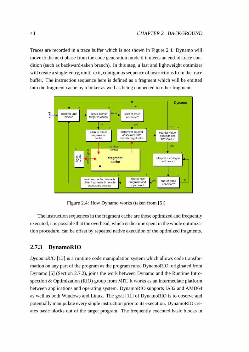
Traces are recorded in a trace buffer which is not shown in Figure 2.4. Dynamo will
move to the next phase from the code generation mode if it meets an end-of-trace con-
dition (such as backward-taken branch). In this step, a fastand lightweight optimizer
will create a single-entry, multi-exit, contiguous sequence of instructions from the trace
buffer. The instruction sequence here is defined as a fragment which will be emitted
into the fragment cache by a linker as well as being connectedto other fragments.
Figure 2.4: How Dynamo works (taken from [6])
The instruction sequences in the fragment cache are those optimized and frequently
executed, it is possible that the overhead, which is the timespent in the whole optimiza-
tion procedure, can be offset by repeated native execution of the optimized fragments.
2.7.3 DynamoRIO
DynamoRIO[13] is a runtime code manipulation system which allows codetransfor-
mation on any part of the program as the program runs. DynamoRIO, originated from
Dynamo [6] (Section 2.7.2), joins the work between Dynamo and the Runtime Intro-
spection & Optimization (RIO) group from MIT. It works as an intermediate platform
between applications and operating system. DynamoRIO supports IA32 and AMD64
as well as both Windows and Linux. The goal [11] of DynamoRIO is to observe and
potentially manipulate every single instruction prior to its execution. DynamoRIO cre-
ates basic blocks out of the target program. The frequently executed basic blocks in

2.7. DYNAMIC OPTIMIZER 45
sequence are stitched together to be a trace. Basic blocks and traces are placed in a
basic block cacheand atrace cache, respectively. Codes running from these caches
behave as if running natively.
The basic infrastructure of DynamoRIO is presented in Figure 2.5. DynamoRIO
considers a sequence of instructions ending with a single control transfer instruction
as a basic block. The basic block of DynamoRIO is different from the traditional basic
block described in Section 2.5.5; its entry and exit points are either a subroutine call, a
return or a branch instruction. A basic block of DynamoRIO usually contains around
6 or 7 instructions, but some basic blocks can reach over 50 instructions. The default
maximum basic block size is 1024. DynamoRIO copies the basicblocks into a basic
block cache from which the instructions can be executed natively. The basic block
cache is a part of memory space. The processor fetches a cacheline from the opti-
mized version of instructions out of the basic block cache. If DynamoRIO detects that
the next target basic block is present in the basic block cache and at the same time can
be targeted by the current executing basic block through a direct branch, DynamoRIO
will link the two blocks together directly. This procedure avoids a time-consuming
and storage-consuming context switch. Acontext switchrefers to the procedure that
saves and restores the general-purpose registers, the condition codes (eflags register)
and any operating system dependent state. Context [15] incorporates the integer reg-
isters, the flag registers, the instruction pointers and theprogram stacks. A context
switch is required when a cache miss occurs and control needsto be transferred back
to DynamoRIO to obtain the required instructions.
Linking direct branches is simple because a direct branch has a unique target. How-
ever an indirect branch incorporates multiple possible targets. DynamoRIO provides
an indirect branch lookup hashtable for referencing the addresses of indirect branches.
The address in the lookup table is not the actual address of the indirect branches, but
one that has already been translated into the basic block cache address. To further im-
prove efficiency and obtain better code layout in the code cache (see Section 2.2), Dy-
namoRIO additionally provides a trace cache. The trace cache occupies a part of cache
space (the physical cache). A trace in the trace cache may have multiple exit points
but it has only one entry point. When a basic block ends with anindirect branch, Dy-
namoRIO retrieves the trace cache before referring to the indirect branch lookup table.
This procedure is much faster than searching the indirect branch lookup table directly.
In DynamoRIO, the data structure of each basic block is a linked list and each instruc-
tion occupies one of its nodes. A basic block is passed as a pointer to a trace. The data
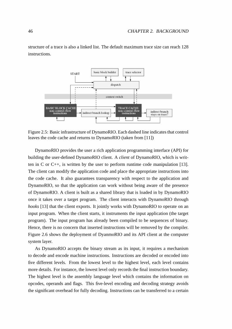
46 CHAPTER 2. BACKGROUND
structure of a trace is also a linked list. The default maximum trace size can reach 128
instructions.
Figure 2.5: Basic infrastructure of DynamoRIO. Each dashedline indicates that controlleaves the code cache and returns to DynamoRIO (taken from [11])
DynamoRIO provides the user a rich application programminginterface (API) for
building the user-defined DynamoRIO client. Aclient of DynamoRIO, which is writ-
ten in C or C++, is written by the user to perform runtime code manipulation [13].
The client can modify the application code and place the appropriate instructions into
the code cache. It also guarantees transparency with respect to the application and
DynamoRIO, so that the application can work without being aware of the presence
of DynamoRIO. A client is built as a shared library that is loaded in by DynamoRIO
once it takes over a target program. The client interacts with DynamoRIO through
hooks[13] that the client exports. It jointly works with DynamoRIO to operate on an
input program. When the client starts, it instruments the input application (the target
program). The input program has already been compiled to be sequences of binary.
Hence, there is no concern that inserted instructions will be removed by the compiler.
Figure 2.6 shows the deployment of DyanmoRIO and its API client at the computer
system layer.
As DynamoRIO accepts the binary stream as its input, it requires a mechanism
to decode and encode machine instructions. Instructions are decoded or encoded into
five different levels. From the lowest level to the highest level, each level contains
more details. For instance, the lowest level only records the final instruction boundary.
The highest level is the assembly language level which contains the information on
opcodes, operands and flags. This five-level encoding and decoding strategy avoids
the significant overhead for fully decoding. Instructions can be transferred to a certain

2.7. DYNAMIC OPTIMIZER 47
Hardware platform
Operating system
DynamoRIO
Running Application
Client
Figure 2.6: The deployment of DynamoRIO and its client (taken from [13])
instruction representative level as needed.
It can be seen that Dynamo and DynamoRIO share some common characteristics.
They both attempt to identify the frequently-executed instruction sequences (traces)
and place them in a code cache. However, DynamoRIO incorporates two code caches,
which are a basic block cache and a trace cache, whereas Dynamo only contains one
code cache which is a fragment cache where the frequently-executed instructions re-
side. The basic block cache in DynamoRIO contains the rest ofthe instruction se-
quence which is used to simplify the code discovery avoidingconstant instructions
transferring between IR and the original input codes. In contrast, Dynamo does not
build basic blocks. Instead it simply suspends the fragmentcache and transfers con-
trol back to the operating system and makes the instructionsexecute in a normal
way. DynamoRIO also contains an indirect branch lookup table for addressing indirect
branches. These additional constituents further improve the performance of the pro-
gram if the additional time overhead of building them can be ignored. In fact, Derek L.
Bruening [13] claims that the majority of direct runtime overhead comes from handling
indirect branches. Even when an indirect branch is inlined into a trace, a comparison
is still needed to ensure that the dynamic branch stays in thetrace. This is achieved
by inserting a check to compare the actual target of the branch with the target that will
keep it on the trace. If the check fails, the trace is exited.
The application of DynamoRIO is not restricted to code optimization. Google
uses DynamoRIO together with Dr Memory to detect memory bugs, such as memory
leaks or shadow memory [12]. DynamoRIO has also been exploited to monitor system
security [28]. For instance, suspicious and malicious applications can be terminated
by DynamoRIO. Zhaoet al. [46] propose an application making use of DynamoRIO
to present the detailed execution profile (DEP). DynamoRIO also shows significant
performance on efficiently analysing interactions betweenthreads to determine thread
48 CHAPTER 2. BACKGROUND
correlation and detect true and false sharing [45]. Other applications of DynamoRIO
can be found on the official web site of DynamoRIO.4
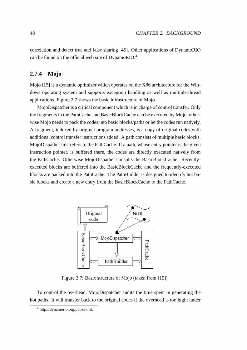
2.7.4 Mojo
Mojo [15] is a dynamic optimizer which operates on the X86 architecture for the Win-
dows operating system and supports exception handling as well as multiple-thread
applications. Figure 2.7 shows the basic infrastructure ofMojo.
MojoDispatcher is a critical component which is in charge ofcontrol transfer. Only
the fragments in the PathCache and BasicBlockCache can be executed by Mojo, other-
wise Mojo needs to pack the codes into basic blocks/paths or let the codes run natively.
A fragment, indexed by original program addresses, is a copyof original codes with
additional control transfer instructions added. A path consists of multiple basic blocks.
MojoDispather first refers to the PathCache. If a path, whoseentry pointer is the given
instruction pointer, is buffered there, the codes are directly executed natively from
the PathCache. Otherwise MojoDispather consults the BasicBlockCache. Recently-
executed blocks are buffered into the BasicBlockCache and the frequently-executed
blocks are packed into the PathCache. The PathBuilder is designed to identify hot ba-
sic blocks and create a new entry from the BasicBlockCache tothe PathCache.
Figure 2.7: Basic structure of Mojo (taken from [15])
To control the overhead, MojoDispatcher audits the time spent in generating the
hot paths. It will transfer back to the original codes if the overhead is too high; under
4 http://dynamorio.org/pubs.html.
2.7. DYNAMIC OPTIMIZER 49
such a condition the codes will run natively. NtDLL is the dynamic linked library of
the Windows system that can be utilised by multiple processes. When control returns
to the application asynchronously, execution re-enters the user-mode through NtDLL.
NtDLL will not return control back to the application until the machine state is set up.
Mojo works well on some small applications and two SPEC CPU 20005 bench-
marks (mcf andcompress95). Similar to DynamoRIO, Mojo also tries to find the hot
instructions and execute them from the fast code cache (called PathCache in Mojo).
But Mojo does not care about the direct branches or indirect branch it encounters, it
plants basic blocks from recently executed instruction sequences and further forms the
path out of hot basic blocks.
2.7.5 Wiggins/Redstone
Wiggins/Redstone [18] is an experimental dynamic optimizer, which makes use of
hardware sampling together with software instrumentationto dynamically collect hot
path/trace information.
Depending on a hardware PC sampler, Wiggins/Redstone identifies hot instruc-
tions. These frequently-executed instructions are copiedto a side buffer6 and form
traces continuously. Wiggins/Redstone continues to identify the hot traces from the
buffer and further optimize them.
Wiggins/Redstone is also a trace-based optimizer like Dynamo and DynamoRIO,
but it relies on hardware to determine which instructions need to be placed in the code
cache.
2.7.6 Java Virtual Machine and JIT compiler
Java Virtual Machine (JVM)7 is software which provides an environment/platform in
which Java bytecodes run. JVM is responsible for interpreting bytecodes and translat-
ing them where necessary into operating system calls.
The latest JVM usually offers Just-In-Time compilation in multiple execution modes
[40]. These systems exploit interpreters or baseline compilers as the first execution
mode [40]. A sampling profiler is employed in this mode to snoop the hot spots. When
5 SPEC CPU2000 is an early published benchmark suite, the later version is SPEC CPU2006 asdescribed in Section 3.2.1.
6 A side buffer in Wiggins/Redstone is equivalent to a code cache.7 JVM, available from http://docs.oracle.com/javase/specs/jvms/se7/html/jvms-1.html, accessed on
17/04/2012.

50 CHAPTER 2. BACKGROUND
the frequently executed spots are detected, the system switches to the next mode which
utilises an optimizing compiler for higher performance. Inthis mode, the recompila-
tion controller determines which spots needed to be recompiled. Based on the informa-
tion obtained from a sampling profiler (a sampling profiler only in charge of detecting
the hot spots and incrementing a hotness counter associatedwith each spot), the con-
troller also decides the optimization level the codes should adapt to. The threshold of
the hotness count matters a lot. The detailed profile information (such as the distribu-
tion of call sites and parameter values) is collected by an instrumenting profiler to feed
back to the recompilation controller. Figure 2.8 shows where the JVM resides and its
working environment.
Java Runtime Environment
Java API class JVM
Operating System
Hardware
Figure 2.8: How JVM works
The Just-In-Time compiler from IBM cooperates with the JVM to improve the
performance of Java applications at run time. IBM’s JVM runswith JIT enabled by
default. IBM’s JIT compiler works in five stages:8 inlining, local optimization, control
flow optimizations, global optimizations and native code generation. A JIT compiler
often incorporates a Mix Mode Interpreter (MMI) [40]. The traditional JIT compiler
employs a method-based optimizing compiler, but it shows its limitation when tack-
ling programs with largely flat profiles.9 A trace-based JIT compiler [26] has been
developed which demonstrates the benefits by forming largerscopes than a method-
based compiler, even in cold spots of a program. This compiler aims to identify the hot
spots and optimize them. In contrast to this technology, a Region-Based Compilation
Technique designed for a JIT compiler [41] attempts to identify the rarely-executed
portions of a program and remove them from the original code so that the compiler
only concerns itself with optimization of the frequently executed portions. A region
8 Available from http://publib.boulder.ibm.com/infocenter/iseries/v5r3/index.jsp?topic=%2Frzaha%2Fjit.htm,accessed on 25/05/2012.
9 Flat profile refers to a profile with a large number of methods that are almost equally important.

2.7. DYNAMIC OPTIMIZER 51
here refers to a compilation unit which results from collecting codes from executed
methods but excludes all rarely executed portions of the methods [41].
The differences between DynamoRIO and the IBM JIT compiler are as follows:
• DynamoRIO creates two types of fragments which are basic blocks and traces. A
basic block is single entry and single exit and a trace is single entry and multiple
exits. A region of JIT compiler only has single-entry and single-exit block (for
a Region-based compiler).
• The JIT compiler does not take into account whether a branch is direct or indirect
as DynamoRIO does.
2.7.7 Pin and its JIT compiler
Pin is an instrumentation tool for program analysis such as profiling, performance
evaluation and bug detection [31].Instrumentationis a technology for inserting extra
codes into a program to observe its behaviour: data races, memory system behaviour
and parallelizable loops. Pin provides instrumentation byinserting and optimizing
codes through the JIT compiler. Figure 2.9 shows the basic architecture of Pin. Fig-
ure 2.10 gives a performance comparison between Pin and DynamoRIO. Pin uses a
way for linking indirect branches that is very similar to that of DynamoRIO. However
Pin exhibits three differences from DynamoRIO [31]:
• In DynamoRIO, the whole chain of predicted indirect branches is generated at
once. In contrast, Pin is more flexible, the chain can be modified while the
program is running.
• Pin utilises a local hashtable whereas dynamoRIO creates a global hashtable.
Luk et al. [31] claim that a local hashtable is able to perform at higher perfor-
mance than a global one.
• Pin uses function cloning [17] to accelerate the indirect branches:returns. A
copy of the function is inserted at the call site when it is called. This function
can be cloned to multiple call sites.
The main goal of Pin is not to improve the performance of the application, but to
analyse the program behaviour. Pin involves a JIT compiler so that it demonstrates
some advantages compared with other instrumentation tools. The code cache of Pin is
not used to store the frequently-executed traces, as is the one in DynamoRIO, but to
keep the compiled codes from its JIT compiler.

52 CHAPTER 2. BACKGROUND
Figure 2.9: The basic architecture of Pin (taken from [31])
2.7.8 HDTrans
HDTrans [38, 39], a simple High-performance Dynamic Translator, was initially de-
signed as a supervisor-mode translator for virtual machinesimulation. The source
basic blocks are translated into the corresponding target basic blocks (traces) by HD-
Trans and are stored in a directory called BBdirectory. It isworth to noting that no
attempt is made to optimize target codes except for trace linearization in this translator.
The translation procedure mainly includes translation of unconditional direct branches
(trace linearization), conditional branches, indirect branches andreturn instructions.
They are summarized in the following paragraphs, respectively.
Translation proceeds straight through conditional branches orcall instructions, and
continues until reaching one of the following three types ofinstructions. These in-
structions are an indirect branch, an unconditionaljmp whose destination has been
previously translated or whose destination is statically unknown. If a directjmpwhose
destination has not been previously translated is encountered, thejmp is elided, a di-
rectory entry is added to BBdirectory for the destination and continue translating at
the destination instruction. In the case of acall instruction, the HDTrans proceeds by
translating the instructions past thecall instruction rather than translating the destina-
tion of call. If the destination ofcall is translated, ajmp is inserted into the basic block,
otherwise performing a translation of acall instruction . This scheme is demonstrated
in Figure 2.11 and Figure 2.12. The syntax of the assembly instructions in the two

2.7. DYNAMIC OPTIMIZER 53
figures is AT&T10. $desthas not been translated. As shown in Figure 2.12 thatjmp
is elided and translation continues frommov $30,%ecxinstead of the instructions fol-
lowed directly (these instructions afterjmpare omitted in the picture). The fifth line of
the original instructions (call $proc) is the call instruction whose destination has been
translated, therefore ajmp is performed. The sixth line in Figure 2.11 is copied directly
to the translated codes asadd $4,espis the following instruction ofcall $procand HD-
Trans chooses not to insert the destination instructions ofcall beforeadd $4,esp; this
last instruction is therefore not reachable
(a) Pin
(b) Pin Versus DynamoRIO
Figure 2.10: Benchmarks performance of Pin and DynamoRIO. The pic-tures are from the DynamoRIO tutorial at CGO2012, availablefrom:https://code.google.com/p/dynamorio/downloads/list.
10 There are two common assembly language syntaxes which are Intel and AT&T.
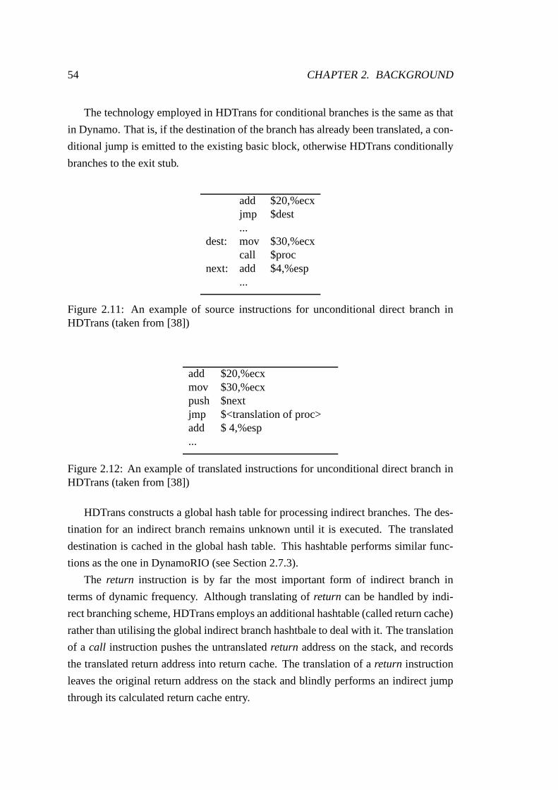
54 CHAPTER 2. BACKGROUND
The technology employed in HDTrans for conditional branches is the same as that
in Dynamo. That is, if the destination of the branch has already been translated, a con-
ditional jump is emitted to the existing basic block, otherwise HDTrans conditionally
branches to the exit stub.
add $20,%ecxjmp $dest...
dest: mov $30,%ecxcall $proc
next: add $4,%esp...
Figure 2.11: An example of source instructions for unconditional direct branch inHDTrans (taken from [38])
add $20,%ecxmov $30,%ecxpush $nextjmp $<translation of proc>add $ 4,%esp...
Figure 2.12: An example of translated instructions for unconditional direct branch inHDTrans (taken from [38])
HDTrans constructs a global hash table for processing indirect branches. The des-
tination for an indirect branch remains unknown until it is executed. The translated
destination is cached in the global hash table. This hashtable performs similar func-
tions as the one in DynamoRIO (see Section 2.7.3).
The return instruction is by far the most important form of indirect branch in
terms of dynamic frequency. Although translating ofreturn can be handled by indi-
rect branching scheme, HDTrans employs an additional hashtable (called return cache)
rather than utilising the global indirect branch hashtbaleto deal with it. The translation
of a call instruction pushes the untranslatedreturn address on the stack, and records
the translated return address into return cache. The translation of areturn instruction
leaves the original return address on the stack and blindly performs an indirect jump
through its calculated return cache entry.

2.7. DYNAMIC OPTIMIZER 55
HDTrans works mainly as a translator, however it embodies dynamic optimization
technology in its infrastructure. HDTrans employs a globalhash table for retrieving
the destination of the indirect branches instead of a trace cache for caching the most-
frequently executed basic blocks. Compared with DynamoRIO, this global hash table
can avoid excessive instruction duplication as well as reducing register pressure and
cache pressure.
2.7.9 Summary
Seven specific runtime optimizers have been surveyed. The dynamic optimizers re-
viewed tend to snoop the frequently executed regions of the program and store them
in some form of code cache. Executing the hot code natively inthe code cache may
accelerate application execution. Dynamic optimizers exploit runtime profile infor-
mation to perform branch prediction and to construct the frequently-executed frag-
ments. DynamoRIO reconstructs the hot basic blocks into traces and executes them
in a trace cache. To overcome the time-consuming procedure for processing indirect
branches, DynamoRIO includes an indirect branch lookup hash table. It will retrieve
the hash table prior to the execution in the basic block cachewhen there is a trace cache
miss. Dynamo performs similar functions as DynamoRIO but only provides one code
cache and lacks an indirect branch hash table. Mojo introduces a basic block cache
for buffering only recently executed blocks. Wiggins/Redstone is an experimental dy-
namic optimizer, which relies on the hardware to speculate which traces are suitable to
reside in the trace cache. The JIT compiler of JVM is a conventional optimizer. It is a
complex system and is developed into different versions which exploit different infras-
tructures. The JIT optimizer combines static and dynamic optimization methods. JIT
compilers fall into two main categories: trace-based compilers and method-based com-
pilers. Pin is developed as a programming analysis tool but it incorporates a structure
based on DynamoRIO for code optimization. The optimizationrationales behind Pin
are similar to DyanmoRIO, however it has been demonstrated that DynamoRIO de-
livers a more significant performance improvement than Pin.HDTrans works mainly
as a translator, however it embodies dynamic optimization technology in its infras-
tructure. HDTrans employs a global hash table for retrieving the destination of the
indirect branches instead of a trace cache for caching the most-frequently executed
basic blocks. Compared with DynamoRIO, this global hash table can avoid excessive
instruction duplication as well as reducing register pressure and cache pressure.

56 CHAPTER 2. BACKGROUND
A dynamic optimizer involves much work on tackling indirectbranches. The desti-
nation of an indirect branch remains unknown until it executes. It is a time-consuming
procedure to process an indirect branch. Therefore the dynamic optimizer employs
prediction algorithms for indirect branches. A dynamic optimizer relies on an impor-
tant principle, which is that a small portion of code occupies the majority of the appli-
cation’s execution time so the performance can benefit from the reuse of instructions
residing in the fragment cache.
2.8 Chapter Summary
This chapter has reviewed relevant background techniques and technologies. It has first
introduced the program analysis methods which are necessary procedures to provide
useful information to guide program optimization. Next, ithas surveyed the method-
ologies for optimization techniques which include software optimization algorithms
and hardware optimization mechanisms. Lastly, it has inspected the basic working
procedures of three important static optimizers and seven dynamic optimizers.
Traditional compilers compile programs once, producing a binary program that
generates correct results under all inputs. Their code optimization depends on static
analyses carried out at compile-time, often at an optimization level selected by the user.
Such optimization technology suffers from inflexibility. Dynamic optimization can
make use of information about the program behaviour while the program runs, thus its
optimization methodology is more flexible than that of static optimization. However,
the overhead caused by runtime optimization operations andsystem initialization must
be offset before any performance improvement is seen. Therefore, static optimization
and dynamic optimization are usually employed in such a way as to supplement each
other.
Profiling techniques and program analysis play an importantrole for analysing and
collecting useful program information to support the choice of program optimization
strategies. Data flow and control flow analysis gains knowledge of the data changes
and control transfers of the whole program. Hence they are widely applied in the com-
piler for program optimization or exploited for programmers to better understand the
program behaviour. A dynamic optimizer needs to generate efficient code to obtain
high performance and reduce the time spent on system initialization and optimization
overhead. This trade-off, between the profile overhead and the performance benefits,

2.8. CHAPTER SUMMARY 57
is a crucial issue for dynamic optimizers [40]. Dynamic optimization requires infor-
mation from the runtime profile to make more accurate prediction and construct the
traces (except that Dynamo does not depend on the runtime profile for trace selection).
The dynamic optimizers tend to exploit a code cache for storing frequently-executed
instruction sequences. The codes run in the code cache can accelerate the execution of
the program.
Comparing the pros and cons of all the optimizers that have been reviewed in this
chapter, DynamoRIO shows significant advantages. Hence, the work described later
in this thesis has used DynamoRIO as the code manipulation system to perform run-
time code analysis and optimization on five carefully selected experiments which are
presented in detail in the next chapter. A static optimization algorithm viewed in Sec-
tion 2.6.2 is revisited in a dynamic context in the next chapter. Also, a modified pro-
gram analysis method from Section 2.4 is presented in the next chapter. Chapter 4 then
summaries the experimental results and discusses future work.
Chapter 3Dynamic Code Analysis and
Optimization
58

Chapter 3
Dynamic Code Analysis and
Optimization
3.1 Introduction
This thesis investigates runtime code manipulation to discover the possible optimiza-
tion strategy and speed up program execution. This chapter presents five experiments
on program analysis and program optimization. Some of theseexperiments, such as
redundanttest instructions removal and instruction alignment, have beencarried out
in static contexts in previous publications but not in a dynamic environment. Some
of these experiments, such as strength reduction and glacial address propagation, are
modifications of previous publications. An overview of the experimental methodology
is presented first in Section 3.2. The chapter then evaluatesthe base performance of
DynamoRIO to gain a brief view of how efficiently it works on code optimization (Sec-
tion 3.3). Next it analyses redundant instruction detection (Section 3.4) and strength
reduction (Section 3.5). Section 3.6 studies runtime instruction alignment analysis
and optimization. Following that, Section 3.7 explains themethod of persistent cache.
Finally, glacial address propagation is investigated and presented in Section 3.8.
3.2 Methodology
Dynamic code optimization introduces a significant runtimeoverhead; this overhead is
expected to be offset by a large amount of efficient code reuse. Therefore, optimization
on the ”cold” regions of a program is not necessary. Code optimization in this chap-
ter is performed on the frequently-executed program regions. Code manipulation and
59

60 CHAPTER 3. DYNAMIC CODE ANALYSIS AND OPTIMIZATION
optimization is performed by the runtime code manipulationsystem DynamoRIO. The
performance of DynamoRIO for dynamic code optimization is evaluated by the exe-
cution time of programs from the SPEC CPU2006 benchmark suite. More details of
SPEC CPU2006 are in Section 3.2.1. The test workload (short-time run) and reference
workload (long-time run) of SPEC CPU2006 are employed for testing effectiveness of
optimization technology. The user defined DynamoRIO clients manipulate the appli-
cation through the interface provided by DynamoRIO. As described in Section 2.7.3,
the user defined clients work together with DynamoRIO to analyse and optimize the
program as it runs. The outcomes (program execution time) are compared with re-
sults of running benchmarks natively (without DynamoRIO).Details of how results
are presented are given in Section 3.3. Running the test workload, few clients demon-
strate performance improvement, as DynamoRIO needs time tobuild the basic blocks,
the traces and the indirect branch hashtable and performingother profiling operations.
This runtime overhead has not yet been offset by performanceimprovement. However,
running the reference workload, more of the benchmarks demonstrate performance
gain because the overhead caused by DynamoRIO is better offset. To guarantee the
performance stability and credibility, the benchmarks areeach tested three times and
the presented results give the average time of the three tests. In Section 3.6, a small
testing program is used for the performance measurement with its error 0.05s. SPEC
CPU2006 is used to measure the performance of computer processor, memory archi-
tecture and compilers. So performance may vary for different hardware and compilers.
3.2.1 Evaluation Test Case: SPEC CPU2006
This section reviews the benchmark suiteSPEC CPU20061, which is widely employed
in academia and industry for evaluating performance of optimization and other tech-
nology. SPEC CPU2006 programs simulate well the behaviour of many kinds of real
applications and are often used as an initial stage to evaluate code optimization meth-
ods or algorithms. A good optimization strategy will lead toperformance gain for
SPEC CPU2006 programs.
SPEC stands for Standard Performance Evaluation Corporation. SPEC is a non-
profit organization, which takes building the standard benchmarks for computer system
as a goal. This organization covers a wide-range of members:computer hardware
vendors, software companies, universities, research organizations, systems integrators,
1 SPEC CPU2006, available from http://www.spec.org/cpu2006/, accessed on 25/05/2012.

3.2. METHODOLOGY 61
publishers and consultants.
SPEC CPU2006 is a benchmark suite that is exploited in this thesis to test the
performance of the dynamic optimization technologies. A software benchmarkis a
computer program that performs set operations, so running the same benchmark on
different platforms allows comparison to be made. SPEC CPU2006 provides a compar-
ative measure of compute-intensive performance across thewidest practical range of
hardware using workloads developed from real end-user applications. SPEC CPU2006
measures the performance of computer processors, memory architecture and compil-
ers. It incorporates INT2006 suite and CFP2006 suite which measure the compute-
intensive integer and compute-intensive floating point performance, respectively.
SPEC CPU2006 also offers three types of workloads, known astest, train andref-
erence, for each benchmark. Thetest workloaddefines a short-run program which is
often used for debugging. This type of workload is a simplified version of the corre-
sponding reference workload, which can usually finish executing in several seconds.
The train workload version takes more time to finish than the test counterpart. The
reference workloadis designed to simulate the function of the real applicationor soft-
ware. Time spent on reference workload is usually more than 10 minutes.
The benchmark packages utilised in this thesis are400.perlbench, 401.bzip2,
403.gcc, 429.mcf, 445.gobmk, 456.hmmer, 458.sjeng, 462.libquantum, 464.h264ref,
471.omnetpp, 473.astarand483.xalancbmk. The primary component of400.perl-
bench is the Open Source spam checking software SpamAssassin. SpamAssassin is
used to score a couple of known corpora of both spam and non-spam, as well as a
sampling of mail generated from a set of random components.401.bzip2simulates
the procedure of file compression and decompression.403.gccsimulates an optimiz-
ing compiler.429.mcf is designed for simulating single-depot vehicle scheduling for
mass public transportation.445.gobmkis designed to play Go and executes a set of
commands to analyse Go positions. The purpose of456.hmmeris to search a gene se-
quence database.458.sjengis designed to simulate chess playing.462.libquantum is
a library for the simulation of a quantum computer.464.h264refis a reference imple-
mentation of the latest state-of-the-art video compression standard.471.omnetppper-
forms discrete event simulation of a large Ethernet network. 473.astaris derived from
a portable 2D path-finding library that is used in computer game’s AI. 483.xalancbmk
is a modified version of Xalan-C++, an XSLT processor writtenin a portable subset of
C++. Table 3.1 summaries all the benchmark packages and introduces the short name
for each package which will be used to refer to it in the remainder of the thesis.

62 CHAPTER 3. DYNAMIC CODE ANALYSIS AND OPTIMIZATION
name short name functionality
400.perlbench perlbench spam checking401.bzip2 bzip2 simulate compression and decompression403.gcc gcc simulate an optimizing C compiler429.mcf mcf simulate single-depot vehicle scheduling445.gobmk gobmk play and execute commands to analyse Go positions456.hmmer hmmer search a gene sequence databases458.sjeng sjeng simulate chess playing462.libquantum libquantum simulate a quantum computer464.h264ref h264ref reference implementation of the video compression standard471.omnetpp omnetpp simulate discrete event of a large network473.astar astar a portable 2D path-finding library483.xalancbm xalancbm a modified version of Xalan-C++
Table 3.1: SPEC CPU2006 packages
3.2.2 Configuration
The performance of the dynamic optimization and analysis strategies in this thesis are
tested by the popular benchmark suites SPEC CPU2006. The performance testing is
carried out on a Pentium(R) dual-core CPU E5700. The operating system version is
Fedora 16 (32 bits). The compiler version is GCC 4.6.3 20120306 (Red Hat 4.6.3-2).
3.3 Base Performance of DynamoRIO
The goal of this section is to demonstrate DynamoRIO’s base performance on runtime
program analysis and optimization. In this section, the application is controlled by
the default user defined clients provided with DynamoRIO. The user clients and Dy-
namoRIO cooperate to analyse and optimize the program as it executes. The default
user clients presented in this thesis include:empty.c, bbsize.c, bbcount.c, inc2add.c
andinline.c. They either perform code optimization or runtime program analysis. To
be more exact,empty.c makes DynamoRIO do basic operations.bbsize.candbb-
count.c are two simple program analysis clients, which are used to observe the size
information of the basic block and how many basic blocks are executed. In2add.c
is a program optimization client, which may speed up programexecution on certain
Intel cores.inline.c is an instrumentation client to perform code inlining whichinlines
entire callees into traces. The functionality of each client is listed in Table 3.2, which
also introduces short client names that will be used in the remainder of the thesis.
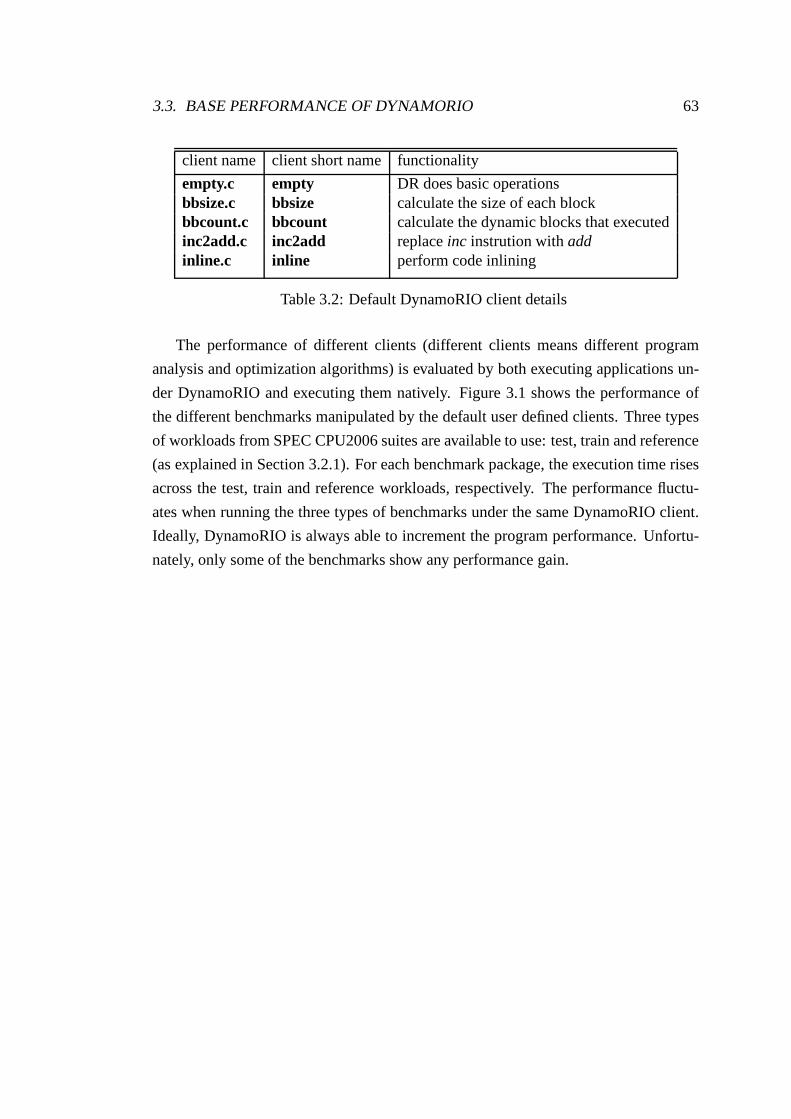
3.3. BASE PERFORMANCE OF DYNAMORIO 63
client name client short name functionality
empty.c empty DR does basic operationsbbsize.c bbsize calculate the size of each blockbbcount.c bbcount calculate the dynamic blocks that executedinc2add.c inc2add replaceinc instrution withaddinline.c inline perform code inlining
Table 3.2: Default DynamoRIO client details
The performance of different clients (different clients means different program
analysis and optimization algorithms) is evaluated by bothexecuting applications un-
der DynamoRIO and executing them natively. Figure 3.1 showsthe performance of
the different benchmarks manipulated by the default user defined clients. Three types
of workloads from SPEC CPU2006 suites are available to use: test, train and reference
(as explained in Section 3.2.1). For each benchmark package, the execution time rises
across the test, train and reference workloads, respectively. The performance fluctu-
ates when running the three types of benchmarks under the same DynamoRIO client.
Ideally, DynamoRIO is always able to increment the program performance. Unfortu-
nately, only some of the benchmarks show any performance gain.
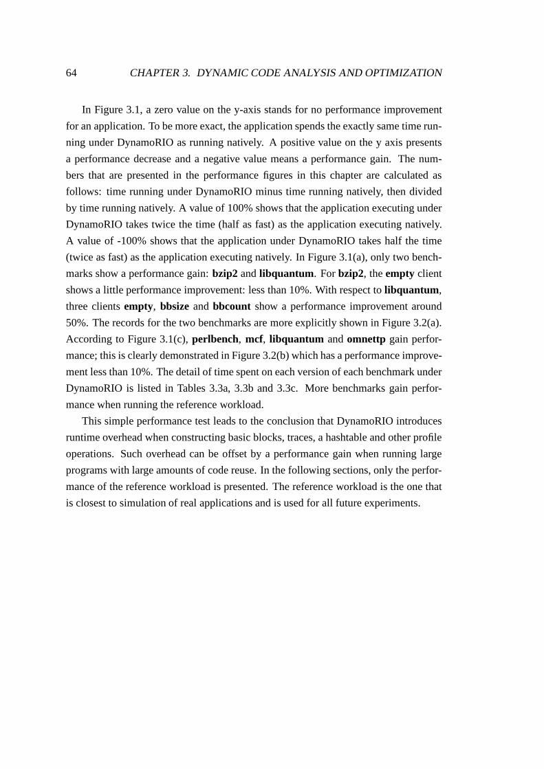
64 CHAPTER 3. DYNAMIC CODE ANALYSIS AND OPTIMIZATION
In Figure 3.1, a zero value on the y-axis stands for no performance improvement
for an application. To be more exact, the application spendsthe exactly same time run-
ning under DynamoRIO as running natively. A positive value on the y axis presents
a performance decrease and a negative value means a performance gain. The num-
bers that are presented in the performance figures in this chapter are calculated as
follows: time running under DynamoRIO minus time running natively, then divided
by time running natively. A value of 100% shows that the application executing under
DynamoRIO takes twice the time (half as fast) as the application executing natively.
A value of -100% shows that the application under DynamoRIO takes half the time
(twice as fast) as the application executing natively. In Figure 3.1(a), only two bench-
marks show a performance gain:bzip2 andlibquantum . Forbzip2, theempty client
shows a little performance improvement: less than 10%. Withrespect tolibquantum ,
three clientsempty, bbsize andbbcount show a performance improvement around
50%. The records for the two benchmarks are more explicitly shown in Figure 3.2(a).
According to Figure 3.1(c),perlbench, mcf, libquantum andomnettp gain perfor-
mance; this is clearly demonstrated in Figure 3.2(b) which has a performance improve-
ment less than 10%. The detail of time spent on each version ofeach benchmark under
DynamoRIO is listed in Tables 3.3a, 3.3b and 3.3c. More benchmarks gain perfor-
mance when running the reference workload.
This simple performance test leads to the conclusion that DynamoRIO introduces
runtime overhead when constructing basic blocks, traces, ahashtable and other profile
operations. Such overhead can be offset by a performance gain when running large
programs with large amounts of code reuse. In the following sections, only the perfor-
mance of the reference workload is presented. The referenceworkload is the one that
is closest to simulation of real applications and is used forall future experiments.

3.3. BASE PERFORMANCE OF DYNAMORIO 65
perlbench bzip2 gcc mcf gobmk hmmer sjeng libquantum h264ref omnetpp astar xalancbmk−200%
0
200%
400%
600%
800%
1000%
1200%
1400%
1600%
1800%
time
sp
en
t ru
nn
ing
on
Dyn
am
oR
IO v
eru
s n
ativ
e tim
e
test workload of benchmarks
empty
bbsize
bbcount
inc2add
inline
(a)
perlbench bzip2 gcc mcf gobmk hmmer sjeng libquantum h264ref omnetpp astar xalancbmk0
50%
100%
150%
200%
250%
300%
350%
400%
450%
500%
time
sp
en
t ru
nn
ing
on
Dyn
am
oR
IO v
eru
s n
ativ
e tim
e
train workload of benchmarks
emptybbsizebbcountinc2addinline
(b)
perlbench bzip2 gcc mcf gobmk hmmer sjeng libquantum h264ref omnetpp astar xalancbmk−20%
0
20%
40%
60%
80%
100%
120%
140%
time
sp
en
t ru
nn
ing
on
Dyn
am
oR
IO v
eru
s n
ativ
e tim
e
reference workload of benchmarks
empty
bbsize
bbcount
inc2add
inline
(c)
Figure 3.1: Simple benchmark performance for test, train and reference workloads

66 CHAPTER 3. DYNAMIC CODE ANALYSIS AND OPTIMIZATION
bzip2 libquantum−100%
−50%
0
50%
100%
150%
200%
250%
300%
time
sp
en
t ru
nn
ing
on
Dyn
am
oR
IO v
eru
s n
ativ
e tim
e
test workload of benchmarks
emptybbsizebbcountinc2addinline
(a)
perlbench mcf libquantum omnetpp−20%
0
20%
40%
60%
80%
100%
120%
time
sp
en
t ru
nn
ing
on
Dyn
am
oR
IO v
eru
s n
ativ
e tim
e
reference workload of benchmarks
emptybbsizebbcountinc2addinline
(b)
Figure 3.2: Simple benchmark performance of test and reference workload
3.4 Experiment 1—Removal of Redundant Instructions
The input code stream for DynamoRIO is a binary stream which is generated by the
compiler (e.g. gcc). The compiler cannot remove all redundant instructions through
static analysis due to lacking online information about program behaviour. Hence the
compiler often generates some redundant instructions. Theruntime code manipula-
tion system is able to observe the online program behaviour and make better use of
hardware configurations to learn new optimization algorithms. One of the significant

3.4. EXPERIMENT 1—REMOVAL OF REDUNDANT INSTRUCTIONS 67
benchmarks native empty bbsize bbcount inc2add inline
perlbench 3.7s 14.8s 17.6s 22.4s 16.5s 23.7sbzip2 11.3s 11.08s 11.8s 16.5s 12.2s 12sgcc 1.32s 5.05s 5.75s 7.95s 5.92s 8.52smcf 2.57 2.75 2.78 3.49 2.83 2.78gobmk 20.2 31.9s 31.6s 41.5s 31.3s 35.9shmmer 3.56s 3.95s 3.97s 4.82s 3.96s 3.95ssjeng 4.64s 6.57s 6.3s 10.5 6.29s 6.85slibquantum 0.0617s 0.282s 0.21s 0.286s 0.205s 0.228sh264ref 20.6s 27.7s 27.7s 39.9s 27.8s 26.2somnetpp 0.546s 1.13s 1.13s 1.87s 1.08s 1.31sastar 10.4s 11.1s 11.1s 13.6s 11.1s 11sxalancbm 0.104s 1.07s 1.32s 1.8s 1.19s 1.81s
Table 3.3a: Time spent on each test workload benchmark with and without Dy-namoRIO
redundant instructions istest, such as the instruction sequence shown in Figure 3.3.
add $0x00000004 %edi -> %edi ;test %edi %edi;
Figure 3.3: Redundanttestinstruction
The add instruction has already set the condition codes, so the following test is
redundant and can be removed. This type of optimization is employed in the static
optimizer developed by Hundt, Ret al. [25] to perform some kinds of static optimiza-
tion. MAO (reviewed in Section 2.6.2) findstestinstructions where both operands are
the same registers and wheretesthas a previous instruction. Then it traverses upward,
bypassingmovinstructions. If it finds asub, and, add, or, xor, or sbbinstruction using
the same register astest, it knows the test was redundant.
MAO does not incur any extra runtime consumption for optimizing the code, but
this matters to DyanmoRIO. The code fragments in DynamoRIO are represented as
linked lists which may not occupy a continuous space even in the same fragment.
Traversing a linked list causes too much overhead and this overhead must be offset by
the performance improvement via reducing redundant instructions. Based on the above
reasons, the first step is to traverse the linked list backward for only one position after
a test instruction is identified. Only redundant instructions residing in the traces (the
definition of trace is reviewed in Section 2.7.3 of Chapter 2)are removed. By doing

68 CHAPTER 3. DYNAMIC CODE ANALYSIS AND OPTIMIZATION
benchmarks native empty bbsize bbcount inc2add inline
perlbench 25s 41.9s 42.3s 76.8s 42.2s 43sbzip2 58.1s 62.5 63s 86.6s 63.8s 62.8sgcc 1.15s 3.99s 4.56s 6.24s 4.35s 6.52smcf 19.5s 20.4s 20.2s 23.3s 20.5s 19.8sgobmk 108s 160s 162s 217s 161s 181shmmer 60s 60.3s 60.4s 68.9s 60.4s 60.4ssjeng 141s 184s 183s 314s 183s 186slibquantum 2.55s 2.6s 2.6s 4.63s 2.66s 2.65sh264ref 118s 159s 159s 227s 159s 148somnetpp 73.1s 96.8s 97.3s 171s 97.3s 98.5sastar 131s 134s 133s 160s 133s 132sxalancbm 77.3s 128s 130s 216s 129s 158s
Table 3.3b: Time spent on each train workload benchmark withand without Dy-namoRIO
this, benchmarklibquantum obtains a 3% performance improvement.
Inspired by this result, a deep retrieval algorithm has beendeveloped to better iden-
tify redundant instructions. This algorithm has been implemented in thetestremover
client. When a suitabletest instruction is detected, the client traverses upward the
whole trace, bypassingmov instructions. However, there are significant numbers of
control transfer instructions residing in the traces whichcan be the original application
instructions or extra profiling instructions. Control transfer instructions may lead the
program to jump to other basic blocks and it is hard to tell whether the condition set
by testwill affect other branches or not. So, when it hits a control transfer instruction,
the algorithm terminates backward searching and continuesto detect the next possible
testinstruction.
Figure 3.4 shows the DynamoRIO routine (a hook function) that is called when a
trace is created and it works as an interface to support instrumentation for each trace.
This routine a function declaration in the program.dr_emit_flags_tis one of the in-
ternal enumeration types defined by the DynamoRIO function libraries; it controls the
behaviour of basic blocks and traces. (more detail can be found from DynamoRIO
header file reference.2 void *tag is the beginning address of each trace. Thevoid
*drcontextparameter here is the thread local machine context used by DynamoRIO. A
client treats*drcontextas an opaque pointer and passes it around for use when calling
API routines [13]. instrlist_t *trace is a trace which is a linked list. The parameter
2 DynamoRIO document, available from http://dynamorio.org/ ,accessed on 25/08/2012.

3.4. EXPERIMENT 1—REMOVAL OF REDUNDANT INSTRUCTIONS 69
benchmarks native empty bbsize bbcount inc2add inline
perlbench 637s 635s 639s 1240s 637s 629sbzip2 815s 841s 841s 1160s 836s 840sgcc 506s 618s 622s 941s 624s 658smcf 484s 495s 469s 547s 454s 468sgobmk 579s 577s 801s 1090s 800s 870shmmer 608s 608s 611s 694s 611s 611ssjeng 680s 679s 885s 1530s 887s 931slibquantum 1330s 1320s 1270s 1400s 1270s 1290sh264ref 872s 872s 1090s 1490s 1090s 1140somnetpp 617s 601s 652s 884s 667s 669sastar 691s 699s 702s 822s 698s 625sxalancbm 405s 502s 500s 899s 504s 533s%
Table 3.3c: Time spent on each reference workload benchmarkwith and without Dy-namoRIO
translatingindicates whether this callback is for trace creation (false) or is for fault ad-
dress recreation (true). Whentranslatingis set to be true, DynamoRIO needs to map
codes back to application instructions.
static dr_emit_flags_tevent_trace(void *drcontext, void *tag, instrlist_t *trace, bool translating);
Figure 3.4: DynamoRIO routine for instrumenting in a trace.
Table 3.4 gives the total number oftest instructions detected in all the traces and
the total number of redundanttestinstructions deleted by thetestremoverclient. Fig-
ure 3.5 shows the resulting benchmark performance when removing test from the
traces alongside theempty client both compared with the benchmark performance
running natively. Theempty client of DynamoRIO does not perform additional instru-
mentation for collecting profile information and does not perform additional program
optimization. This client only enables DynamoRIO to finish its basic operations, such
as building basic blocks, traces, hash table andetc. Performance comparison under
empty client with DynamoRIO’s other clients clarifies performance gains or loses ob-
tained by the designed optimization or analysis algorithm.For instance, better per-
formance thanempty client but worse than native execution shows that a program’s
performance is improved but still not enough to offset the overhead caused by Dy-
namoRIO’s initialization. Where appropriate the following experiments in this chapter

70 CHAPTER 3. DYNAMIC CODE ANALYSIS AND OPTIMIZATION
also compare performance of the new clients with DynamoRIO’sempty client as well
as native execution,
benchmarks redundanttest testdetected redundant rate
perlbench 102 11792 0.86%bzip2 36 237 15.18%gcc 470 97276 0.48%mcf 6 270 2.22%gobmk 105 13975 0.75%hmmer 18 694 2.59%sjeng 11 562 1.96%libquantum 1 113 0.88%h264ref 56 6042 0.93%omnetpp 37 1920 1.93%astar 8 504 1.59%xalancbm 13 2789 0.47%
Table 3.4: Total number oftestinstructions detected and deleted bytestremoverclientin the traces of the SPEC CPU2006 benchmarks
perlbench bzip2 gcc mcf gobmk hmmer sjeng libquantum h264ref omnetpp astar xalancbmk−5%
0
5%
10%
15%
20%
25%
30%
35%
40%
time
sp
en
t ru
nn
ing
on
clie
nt
veru
s n
ativ
e t
ime
performance of testremover client
empty client
testremover client
Figure 3.5: Benchmark performance on thetestremoverclient andempty client
3.5 Experiment 2—Strength Reduction
Strength reduction refers to the strategy of substituting an expensive instruction with
its cheaper counterpart. In some cases, X86 instructionlea (load effective address)

3.5. EXPERIMENT 2—STRENGTH REDUCTION 71
performs the same function asadd. For example, the instructions in Figure 3.6 are
equivalent.
add reg, reg, update;lea reg,[reg+update];
Figure 3.6: Equivalent instructions. The two instructionsboth increase the value in regby the same amount:update.
This section presents a replacement algorithm usinglea to substituteadd if lea
updates the register in the above format.lea does not change eflags (the arithmetic
flags) and doing away with the need to save and restore eflags significantly reduces
the overhead due to a context switch [44]. However,lea andadd both only require
one CPU cycle so their execution speed is the same on the processor butlea executes
faster thanadd under DynamoRIO. This could be further extended to any runtime
code manipulation system that needs a context switch. Recall that a context switch is a
procedure of storing and calling the machine states. More details of context switch are
reviewed in Section 2.7.3. The replacement operation is merely applied in the traces,
since the program spends most of its time on them. A further analysis needs to be
done to determine if the eflags variation betweenlea andadd is acceptable for each
trace. To be more specific, when a suitableadd is observed, the algorithm continues
to check subsequent instructions within the trace. If the following instructions need
to read the eflags or an exit control transfer instruction is hit, add is not allowed to
be replaced bylea. In addition,add has two source operands (reg and updateare
two separate operands) butlea has only one ([reg+update] is one operand). Because
of this, the operands merge (merge two operands into one) here for lea needs to be
carefully handled.
The above strength reduction algorithm has been implemented in the add2lea
client, which improves the performance of benchmarkslibquantum andmcf by 3.8%
and 7.6%, respectively. Table 3.5 gives the total number ofadd instructions that reside
in all the traces and the total number ofadd instructions that are replaced bylea by
theadd2leaclient. More detail of the performance results is shown in Figure 3.7. One
thing that needs to be taken into account is that benchmarkgccfails during the testing.
A verified reason for this at the time of writing remains unknown.
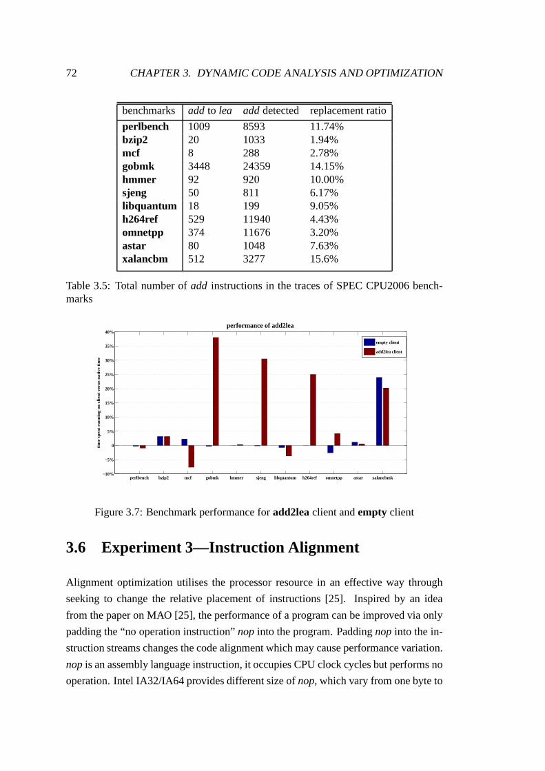
72 CHAPTER 3. DYNAMIC CODE ANALYSIS AND OPTIMIZATION
benchmarks add to lea adddetected replacement ratio
perlbench 1009 8593 11.74%bzip2 20 1033 1.94%mcf 8 288 2.78%gobmk 3448 24359 14.15%hmmer 92 920 10.00%sjeng 50 811 6.17%libquantum 18 199 9.05%h264ref 529 11940 4.43%omnetpp 374 11676 3.20%astar 80 1048 7.63%xalancbm 512 3277 15.6%
Table 3.5: Total number ofadd instructions in the traces of SPEC CPU2006 bench-marks
perlbench bzip2 mcf gobmk hmmer sjeng libquantum h264ref omnetpp astar xalancbmk−10%
−5%
0
5%
10%
15%
20%
25%
30%
35%
40%
time
sp
en
t ru
nn
ing
on
clie
nt ve
rus
na
tive
tim
e
performance of add2lea
empty client
add2lea client
Figure 3.7: Benchmark performance foradd2leaclient andempty client
3.6 Experiment 3—Instruction Alignment
Alignment optimization utilises the processor resource inan effective way through
seeking to change the relative placement of instructions [25]. Inspired by an idea
from the paper on MAO [25], the performance of a program can beimproved via only
padding the “no operation instruction”nop into the program. Paddingnop into the in-
struction streams changes the code alignment which may cause performance variation.
nopis an assembly language instruction, it occupies CPU clock cycles but performs no
operation. Intel IA32/IA64 provides different size ofnop, which vary from one byte to

3.6. EXPERIMENT 3—INSTRUCTION ALIGNMENT 73
nine bytes. In C/C++, an instruction can be considered as anopoperation when it does
not affect the program output. For instance,i+1 or “;” can become anopoperation.
In DynamoRIO, the instructions listed in Table 3.6 are also considered to benop. Dy-
namoRIO also provides several choices for the size of onenop, in this thesis one byte
is selected.
xchg reg,reg;mov reg,reg;lea reg, (reg);
Table 3.6: Equivalent tonop instructions in DynamoRIO
In static optimization, a compiler may remove or generatenopswhen compiling
the source files into the executable. A static compiler inserts alignment instructions
roughly based on the underlying micro-achitecture [25]. For example, insertingnop
to avoid a pipeline hazard and to align a branch target to an 8-byte or 16-byte cache
line. The problem of the alignment strategy is that a compiler just paddingnop into
the branch based on a rough idea about the underlying hardware [25]. In a dynamic
optimizer, more information about underlying hardware maybe available. To inves-
tigate the dynamic situation, firstly a simple clientnopremovehas been designed to
simply delete all thenopsin traces. Other infrequently-executed regions of the pro-
gram are ignored. By doing this operation, it receives 4% and1% performance gain on
benchmarkmcf andlibquantum , respectively. The benchmark performance is shown
in Figure 3.8. DynamoRIO only deletesnop on the fly, after benchmarks finish exe-
cution, the “deleted”nopstill exists in the original code stream. DynamoRIO will not
make changes to the original code, as it makes a copy of all thecodes in the basic block
cache.
In order to test how insertingnop can affect program performance, a small loop-
intensive testing program has been written. This program costs around 2 minutes to
execute. The time error is 0.05 seconds. DynamoRIO automatically builds 15 traces
for this program. Each trace contains no more than 11 instructions. An example of
a trace from this program is shown in Figure 3.9. It is worth noting that, Figure 3.9
is addressed to show the structure of a trace only. This traceis an intermediate code
sequence generated directly by DynamoRIO itself, which canbe a sequence of instru-
mentation codes. It is worth noting that the focus of the picture is to present how a trace
is composed of rather than its actual functionality. This trace has multiple exits. The

74 CHAPTER 3. DYNAMIC CODE ANALYSIS AND OPTIMIZATION
perlbench bzip2 gcc mcf gobmk hmmer sjeng libquantum h264ref omnetpp astar xalancbm−5%
0
5%
10%
15%
20%
25%
30%
35%
40%
tim
e s
pe
nt
run
nin
g o
n c
lie
nt
ve
rus n
ative
tim
e
performance of nopremove
empty client
nopremove client
Figure 3.8: Benchmark performance fluctuation when removing nop instructions inthe hot regions
rightmost column shows the instructions comprising the trace. The instructions are
presented in AT&T format. The middle column is the binary code corresponding to
each assembly instruction.0x416563f8is the beginning address of the trace. The left
column indicates the address increase. The clientnopoptimizer has been implemented
to dynamically insertnopsinto the program. Different numbers ofnopsare inserted
into different positions (in the beginning, in the middle and the second last position) of
each trace. The reasons of such a choice will be stated later in this section. Through
investigating the performance it is observed that the appropriate number ofnopsto pad
into each trace is between 5 and 16. The performance variation whennopsare inserted
into different traces is demonstrated in Figure 3.10. The ordinals in the x dimension
stand for the trace label. For example, 1 represents Trace 1 and 15 represents Trace
15. The performance running under thenopoptimizer client is compared with the
performance under DynamoRIO’sempty client as well as program execution natively.
Theempty client only does limited optimization performed by DynamoRIO itself (for
more detail see Section 3.4). The performance of theempty client always stays on a
level of +6%. Thenopoptimizer VS empty client bars are performance comparison
betweennopoptimizer client andempty client (this is a client comparison, rather than
against native as used everywhere else).
The performance of the program is presented in Figure 3.10 only when anopis in-
serted at the beginning, in the middle and at the second last position of each trace. As
the last instruction of a trace is always a control transfer instruction,nopsinserted after
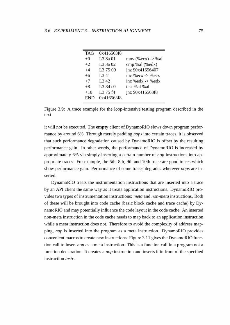
3.6. EXPERIMENT 3—INSTRUCTION ALIGNMENT 75
TAG 0x416563f8+0 L3 8a 01 mov (%ecx) -> %al+2 L3 3a 02 cmp %al (%edx)+4 L3 75 09 jnz $0x41656407+6 L3 41 inc %ecx -> %ecx+7 L3 42 inc %edx -> %edx+8 L3 84 c0 test %al %al+10 L3 75 f4 jnz $0x416563f8END 0x416563f8
Figure 3.9: A trace example for the loop-intensive testing program described in thetext
it will not be executed. Theempty client of DynamoRIO slows down program perfor-
mance by around 6%. Through merely paddingnopsinto certain traces, it is observed
that such performance degradation caused by DynamoRIO is offset by the resulting
performance gain. In other words, the performance of DynamoRIO is increased by
approximately 6% via simply inserting a certain number ofnop instructions into ap-
propriate traces. For example, the 5th, 8th, 9th and 10th trace are good traces which
show performance gain. Performance of some traces degradeswherevernopsare in-
serted.
DynamoRIO treats the instrumentation instructions that are inserted into a trace
by an API client the same way as it treats application instructions. DynamoRIO pro-
vides two types of instrumentation instructions:metaandnon-metainstructions. Both
of these will be brought into code cache (basic block cache and trace cache) by Dy-
namoRIO and may potentially influence the code layout in the code cache. An inserted
non-meta instruction in the code cache needs to map back to anapplication instruction
while a meta instruction does not. Therefore to avoid the complexity of address map-
ping, nop is inserted into the program as a meta instruction. DynamoRIO provides
convenient macros to create new instructions. Figure 3.11 gives the DynamoRIO func-
tion call to insertnopas a meta instruction. This is a function call in a program nota
function declaration. It creates anop instruction and inserts it in front of the specified
instructioninstr.

76 CHAPTER 3. DYNAMIC CODE ANALYSIS AND OPTIMIZATION
1 2 3 4 5 6 7 8 9 10 11 12 13 14 15−10%
−5%
−0
5%
10%
15%
20%
25%
time
imap
ct
nop inserting at the front of each trace
each traceempty clientnopoptimizer VS empty client
(a)
1 2 3 4 5 6 7 8 9 10 11 12 13 14 15−10%
−5%
−0
5%
10%
15%
20%
25%
time
imap
ct
nop inserting in the third position of each trace
each traceempty clientnopoptimizer VS empty client
(b)
1 2 3 4 5 6 7 8 9 10 11 12 13 14 15−10%
−5%
−0
5%
10%
15%
20%
25%
time
impa
ct
nop inserting in the second last position of each trace
each trace
empty client
nopoptimizer VS empty client
(c)
Figure 3.10: Performance fluctuation whennopsare padded into different positionsof each trace compared with running the program natively andrunning under Dy-namoRIO’s empty client
3.6. EXPERIMENT 3—INSTRUCTION ALIGNMENT 77
instrlist_meta_preinsert(trace,instr,INSTR_CREATE_nop(drcontext));
Figure 3.11: A DynamoRIO function call for insertingnopas a meta instruction
3.6.1 Analysis of Rationales fornop Optimization
According to previous research [25], the identified and speculative rationales thatnop
can make an effect on program performance are summarized as follows:
• Intel core micro-architecture (core i3, core i5 and core i7)[2] comprises a Loop
Stream Detector (LSD), which can detect small loops in the program and lock
them in a double buffer (which resides in CPU). This double buffer is able to
hold two 16-byte chunks of data. LSD can bypass instruction fetching, decoding
or reading under certain circumstances. This takes advantage of avoiding repeat-
edly decoding the same instructions and making the same branch predictions. If
a loop contains no more than 18 instructions (excluding thecall instruction ),
executes at least 64 iterations, does not span over four 16-byte decoding lines
(requires only up to 4 decoder fetches of 16 bytes) and incorporates at most 4
taken branches, then the loop may be locked in the instruction queue and there-
fore more quickly available when the loop is used again. The requirements may
vary for different vendors. Paddingnopsmay lead a loop to meet the require-
ments for invoking LSD. Many calculation intensive loops, searches and soft-
ware string moves match the above characteristics, which can be easily affected
by noppadding.
• Insertingnopmay change the branch prediction of the processor. Several condi-
tional branches may be mapped to the same entry of the branch prediction pattern
table. Each entry in this table gives the information of taken or not taken. There
is a high possibility that several branches may share the same branch prediction
entry which cause the prediction outcomes to interfere witheach other. Suppos-
ing branch a and branch b share the same entry in the pattern table, branch a
is always not taken and branch b is always taken. In the worst case, the taken
and not-taken branches are executed alternately. Thereby the taken branch is
predicted based on the outcome of the fall-through branch and vice versa. By
insertingnops, the odds of such interference among branches may be reduced.

78 CHAPTER 3. DYNAMIC CODE ANALYSIS AND OPTIMIZATION
• x86/64 Core-2 decodes instructions in 16-byte chunks. Aligning a loop at a 16-
byte chunk results in decoding of one line instead of two.
• Paddingnopsmay affect data dependences in the pipeline.
As a consequence of the above, it may be helpful to insert pseudo-random num-
bers ofnop instructions into a program. The idea [25] behind this (inserting random
number ofnops) is that codes get shifted around to expose micro-architectural cliffs
via inserting instructions. This may result from removing unknown alias constraints
or limitations in the branch predictor, however this is a speculative reason which needs
to be further investigated. Also it is still not clear that how many numbers ofnops
to layout are able to make best use of the underlying processor architecture, thus en-
abling program optimization. In the following sections, the maximum number ofnops
inserted are 15 occupying 15 bytes. As stated above, processors tends to organize in-
structions into 16-byte chunks, therefore inserting less than 16-bytenopsmay trigger
its optimization mechanism and speed up program.
However, paddingnopcan also cause performance degradation which in fact hap-
pens with a high possibility. Insertingnopsin a program brings more instructions in the
program and a larger instruction cache footprint. This may degrade program perfor-
mance, but it is expected that this degradation can be covered by any performance gain
due to above reasons. According to the above reasons, the nop_optimizer approach is
highly hardware-dependent. Performance will certainly bedifferent when running the
nopoptimizer client on a different platform.
Through testing the small specified program, an overview hasbeen obtained of how
paddingnopsinto the frequently-executed regions in the program can make changes to
its performance. In following sections, this idea is applied to programs from the SPEC
CPU2006 benchmark suite. In order to find out the appropriatetraces for insertingnop,
three instrumentation clients have been investigated to collect the online profile infor-
mation, namely:MemoryReference, BranchTarget andCacheSimulator. However,
no performance results are presented for the first two clients. MemoryReferenceand
BranchTarget do not work efficiently to collect the required expected profile informa-
tion, due to limitations in DynamoRIO.
3.6.2 Memory References Simulator
Memory reference in this section is an address for instructions only. It includes direct
addresses and indirect addresses. A direct address specifies an address by a constant

3.6. EXPERIMENT 3—INSTRUCTION ALIGNMENT 79
value. An indirect address specifies an address by either a register or a combination
of registers and constant values. TheMememoryReferenceclient collects informa-
tion about memory references for each trace. The information, such as memory write
reference and memory read reference, is collected before and after paddingnop. The
idea is that, when the total number of memory references varies, this means thatnops
influence memory accesses. As the number of memory references can be profiled for
each trace, and this makes it possible to select traces that are significantly affected by
insertingnops.
Figure 3.12 gives the DynamoRIO function calls that are utilised to determine if
an instruction is a memory reference (memory read or memory write). instr in the
brackets here represents an instruction which is a pointer in DynamoRIO. However, no
memory reference change is detected after insertingnopinto the traces. This operation
is constrained by DynamoRIO itself. DynamoRIO only considers instructions whose
operand is a memory access address as a memory reference. Sincenophas no operand,
it is not considered as a memory reference by DynamoRIO even thoughnopstill needs
to be stored in the memory.
instr_reads_memory(instr);instr_writes_memory(instr);
Figure 3.12: The DynamoRIO calls to determine memory references. The two instruc-tions are function calls not function declaration.
3.6.3 Branch Target Prediction Simulator
Apart from memory access, branch prediction is the main factor for slowing down
the processor in the case of misprediction. DynamoRIO simply utilises a hardware
branch prediction mechanism known as Branch Target Buffer to perform the branch
prediction and inlines a frequently taken branch into the trace. Branch prediction has
been reviewed in Section 2.5.4 (for more information on Branch Target Buffer, refer to
Intel manual [2]).
As discussed before, paddingnopinto codes containing branches may influence the
branch predictor of the Intel platform. The idea in this section is to collect the branch
target addresses3 before paddingnop and the branch target addresses after padding
3 The target address of a branch where the branch will jump to.

80 CHAPTER 3. DYNAMIC CODE ANALYSIS AND OPTIMIZATION
nop. Several branch instrumentation routines that are provided by DynamoRIO can
be exploited to investigate whether or not the branch targetpredictions are affected by
paddingnopprior to the control transfer instructions. DyanmoRIO provides four types
of branch instrumentation function calls which are listed in Figure 3.13.
dr_insert_call_instrumentation();dr_insert_ubr_instrumentation();dr_insert_mbr_instrumentation();dr_insert_cbr_instrumentation();
Figure 3.13: The DynamoRIO branch instrumentation function calls
These routines insert a clean call4 prior to the control transfer instructions and pass
the instruction PC and target PC as well as the taken or not taken information for
conditional branches to the callee (a user-defined function). The first routine is used
for passing two arguments: address of call instruction and target address of call. The
second routine is used for passing two arguments: address ofbranch instruction and
target address of branch instruction. The third routine is used for passing address of
branch instruction and target address of branch. The last routine is used for passing
three arguments: address of branch instruction, target address of branch instruction
and taken or fall-through information. In theBranchTarget client, a thread event
from DynamoRIO is invoked to dump target addresses, branch target addresses and
the information of whether branches are taken or not to a log file for later inspection.
There are also two global counters set for the total branch hits and branch misses of
the program.
However, the branch target addresses that DynamoRIO can obtain are the instruc-
tion addresses, not the code cache addresses. The instruction addresses will not be
changed due to inserting a meta or non-meta instruction, although it is achievable to
insert a non-meta instruction and make it execute together with the application in-
structions, so that the code cache addresses can be collected. But the code cache ad-
dress of an application branch jump target remains unknown due to a constraint of
DynamoRIO. DynamoRIO links and unlinks the target dynamically to point to differ-
ent fragments. Also the layout of code cache will be disturbed by inserting meta and
4 A clean call in this section inserts into a trace prior to where meta-instruction(s) to save state fora call, switch to this thread’s DynamoRIO stack, set up the passed-in parameters, make a call to callee,clean up the parameters, and then restore the saved state.

3.6. EXPERIMENT 3—INSTRUCTION ALIGNMENT 81
non-meta instructions. As a consequence of the above reasons, this branch target pre-
diction client does not detect any branch mis-prediction rate change nor the instruction
address changes after paddingnop into the traces.
3.6.4 Cache Simulator
Th CacheSimulatorclient simulates the behaviour of a hardware cache. In this section
the cache simulator is limited to be a fully associative instruction cache. The most
commonly-used cache line replacement algorithms FIFO (First In First Out) and LRU
(Least Recently Used) are employed. The FIFO cache line contains two parts, namely
a tag and a valid bit. A tag in this cache simulator is specifiedas a dynamic address of
an instruction in the trace cache. An LRU cache line containsone more segment which
is a counter or timer. This local counter in the cache line is updated by a global counter
every time a cache access happened. To be more specific, the global counter increases
every time a cache access happens. When a cache hit happens, the local counter of a hit
cache line is replaced by the global counter. When a cache miss happens, DynamoRIO
creates a new cache line and sets the value of its local counter to be the value of the
current global counter. In this way, it can be guaranteed that the least recently used
cache line can be swapped out of the cache block when cache is full but a new cache
line will not be swapped out immediately
As in the previous experiment,nopsare padded only in the traces. They are inserted
in front of the control transfer instructions, which may potentially change the target
addresses of the control transfer instructions and cause the cache lines to change. The
cache hit and cache miss for each trace and the whole program are recorded to find out
whether the program’s performance is affected by insertingnopand to decide which
trace is an appropriate trace for insertingnop.
Two global counters are used to record the cache misses and cache hits for the
whole program and export them in the standard output stream of DynamoRIO. Two
local counters are also set to record the cache misses and cache hits for each trace. The
information for each trace is dumped into a log file for later inspection. A thread is
generated every time a trace finishes execution, to record the cache misses and hits of
each trace. The thread exports the results into a log file every time a trace finishes ex-
ecution. The thread is initialised and terminated by the routines shown in Figure 3.14.
The thread initialisation and termination routines are hook functions.
The experiment results for theCacheSimulator client show the following. The

82 CHAPTER 3. DYNAMIC CODE ANALYSIS AND OPTIMIZATION
void event_thread_init(void *drcontext);void event_threead_exit(void *drcontext);
Figure 3.14: Thread initialisation and termination routines
FIFO cache line replacement algorithm causes frequent cache misses. The cache sim-
ulator becomes busy when the program starts to run for a whileand reaches its size
limit. The old cache lines are swapped out frequently, especially when insertingnops
into each trace, asnopsalso occupy the cache line. Insertingnopsin each trace of the
benchmarks greatly increases the whole cache miss rate. Forexample, before inserting
nops, libquantum has 5% cache miss rate, but after inserting 15nops(the reasons for
the choice of the numbers are stated in Section 3.6.1) in front of every control transfer
instruction in each trace, the cache miss rate rises to be 46%. However, the cache miss
rate decreases in certain traces after insertingnops. The cache simulator helps to de-
cide the good traces in which to insertnop, which are the ones that cause fewer cache
misses.nopsare padded in front of every control transfer of the selectedtrace instruc-
tions. By doing this,libquantum shows 2% performance improvement. Paddingnops
does not have any obvious effect on the performance ofgccor perlbench.
The LRU cache replacement algorithm does not cause as much cache miss rate
as FIFO does. Traces are the frequently-executed codes thatare linked together to
achieve better performance. So, in each trace, the instructions executed are very likely
to be called soon and will not be swapped out of the cache. Padding nopsinto each
trace in front of every control transfer instruction actually decreases the cache miss
rate, however this may be caused by the size of the simulated cache. The good traces
detected under LRU are almost the same as the good traces detected under FIFO, which
show lower cache miss rate after paddingnops.
The disadvantage of theCacheSimulatorclient is that it requires a large amount
of time to finish. This may be not acceptable to apply for a realapplication, as real
applications tend to be larger than the benchmark suite. However, this strategy is
approachable and currently the only way that DynamoRIO can be employed to detect
the effect ofnop. The reason that the performance oflibquantum is affected maybe
due to its CPU-intensive operations. CPU-intensive programs are more likely to be
affected by the optimization algorithms targeting the processor, either by making better
use of the superscalar or branch prediction or LSD of the processor.

3.7. EXPERIMENT 4—PERSISTENT CODE 83
3.7 Experiment 4—Persistent Code
Dynamic code optimization works well for long-running applications with a significant
amount of code reuse. But, for short-running applications or long-running applications
with little code-reuse, it is not a good idea to apply online optimization because the
time speed-up cannot offset the runtime overhead. In such cases, the optimized ver-
sion of the application can be stored on disk and reloaded directly the next time the
application is called. Thereby, subsequent executions of the application can be much
faster with little instrumentation overhead. This sectiononly investigates techniques
on persistent codes and presents a simple clientpersistcodeto show performance of
the persistent code.
To achieve persistent code in the context of DynamoRIO, the user needs to set
DynamoRIO’s runtime flags-persist and-persist_dir. The-persist flag enables per-
sisting of the code caches by storing to the disk, while-persist_dir sets the directory
where the persistent code expected to be stored. By default in DynamoRIO, codes
are not persistent. It is required to backup the state of the code cache the first time
the application executes and restore it when the application executes again under Dy-
namoRIO. The function calls provided by DyanmoRIO that enables users to cache the
different types of data in the persistent file are shown in Figure 3.15.
dr_register_persist_ro();dr_register_persist_rx();dr_register_persist_rw();dr_register_persist_patch();
Figure 3.15: DynamoRIO calls to enable 4 types of data to be saved in persistent cache
The first function enables the client to store read-only data, the second one enables
the client to add executable code, the third one enables the client to tackle the writable
data and the last one to patch the codes. Only the optimized basic blocks can be stored
to the disk and reloaded directly by DynamoRIO.
The code optimization strategies are applied to the basic blocks due to the limita-
tion of DynamoRIO. DynamoRIO only enables persistent code for basic blocks. The
return value of the basic block event is set to be: DR_EMIT_PERSISTABLE, instead
of DR_EMIT_DEFAULT to inform DynamoRIO that the basic blockneeds to be per-
sistent. There is not too much investigation of persistent code optimization in this sec-
tion, because the system consumes a large amount of time to backup the environment

84 CHAPTER 3. DYNAMIC CODE ANALYSIS AND OPTIMIZATION
parameters and application codes as well as the profile codes. The approach, persistent
cache, is found more adequate and widely used for static optimization rather than ap-
plying in a dynamic environment. Figure 3.16 shows the performance of the persistent
code. The blue columns (the left-hand ones) represent the application running at the
initial step and the red columns (the right-hand ones) represent the application being
reloaded and run a subsequent call. The system shows a slighttime decrease in a sub-
sequent run. Conclusion appears to be that the cost of reinstalling the persistent code
without any optimization is almost the same as the original cost for instrumentation to
make persistent code.
Perlbench bzip2 gcc mcf gobmk hmmer sjeng libquantum h264ref omnetpp astar xalancbmk0
50%
100%
150%
200%
250%
300%
350%
400%
450%
500%
time
spen
t run
ning
on
clie
nt v
erus
nat
ive
time
performance of persistent cache
inital step
second call
Figure 3.16: Persistent code performance comparison between that of the initial stepand that of the second call. Persistent code is constructed in the initial step and isreloaded to execute under DynamoRIO in the second call
3.8 Experiment 5—Glacial Address Propagation
Some variables, whose values change sufficiently slowly in execution of the program,
are qualified to be worth generating special case code, in which the value is treated as
a constant for a period, thus enabling a cascade of optimization. Such variables are
called glacial variables [4]. This type of analysis is a modification the constant prop-
agation optimization algorithm. Background information on glacial variable analysis
and constant propagation analysis is reviewed in Section 2.4. Since glacial variable
analysis largely relies on runtime profile information, this makes it impossible for a
static compiler to perform during compile time. In spite of the promise of existing

3.8. EXPERIMENT 5—GLACIAL ADDRESS PROPAGATION 85
work, glacial variable analysis has not been widely exploited, since it has been diffi-
cult to imagine a mechanism whereby the information about glacial values, necessarily
obtained at runtime, is fed back to a compiler. In this section, the main goal of glacial
variable propagation is to detect the potential glacial variables in a program, and dis-
cover the opportunity for runtime code optimization; therefore the program execution
time is temporarily ignored. DynamoRIO has no notion of variables other than ad-
dresses, however indirect addresses are variables at the assembly language level. The
goal of glacial address propagationin this section is to label the indirect addresses
with useful properties to aid selection of cost-effective and value-specific optimiza-
tion. TheGlacialVariable client has been designed and implemented to perform this
analysis.
3.8.1 Constant Addresses Analysis
Constant propagation is usually employed in a compiler and is easy to perform at the
high-level language or IR level. A constant address enablesthe processor to make bet-
ter use of the instruction pipeline and branch prediction. Table 3.7 shows an example
of two potential indirect address candidates which could bereplaced by address con-
stants, and Table 3.8 shows the substitution of the candidate instructions. The assembly
language instructions here are presented in Intel format. For the two instructions in Ta-
ble 3.7, their operands contain indirect addresses which could be replaced by constant
addresses. To be more exact, the operanddword ptr [eax+0x50] gives the content
at the address computed by taking the content in registereax plus 0x50. Therefore
the computed address (assuming the computed address is 0x06) can be replaced by a
constant address0x06. The operandedi is an indirect address whose content is an ad-
dress, therefore the registeredi could be replaced by the constant address0x4ce74008
(assuming the address stored in the register is 0x4ce74008). The values of the con-
stant addresses are based on the previous instructions executed. For example, if the
value in the registeredi stays the same as0x4ce74008, then the register operand can
be replaced with the constant value0x4ce74008.
mov ecx, dword ptr [eax+0x50];jmp [edi];
Table 3.7: An example of indirect address candidates
86 CHAPTER 3. DYNAMIC CODE ANALYSIS AND OPTIMIZATION
mov ecx,[0x06];jmp 0x4ce74008;
Table 3.8: An example of substitution instructions for the instructions in Table 3.7
Analysis of glacial addresses is a modification of the glacial variable analysis (see
Section 2.4 for more details) proposed by Autreyet al. [4]. Instead of analysing
variables, memory addresses are taken into account, as variables are expressed as ad-
dresses at the assembly language level. The same as in [4], the analysis is divided into
the following two steps:
• distinguish a program into different special parts based onsome conditions. In
this section, such a special part is addressed as astage. Within a stage, it is com-
posed of several basic blocks. A basic block with a stage is called astage level.
• analyse the change frequency of the indirect memory addresses in each labelled
stage level (basic blocks) of its corresponding stage.
To be more exact, the whole program is distinguished into many stages. Within
a stage the basic blocks are numbered as stage levels starting at stage level 0 when
each time a new stage begins. One basic block is one stage level. Recall that each
basic block in DynamoRIO is a sequence of instructions ending with a control transfer
instruction. A basic block could be executed multiple timescontiguously but is only
regarded to be one stage level. It is worth noting that a stagecan also repeat multiple
times. Figure 3.17 shows how a stage is constructed. A basic block ending with an
indirect call (call via a register) or direct call (call via aprocedure name) is a possible
candidate of Stage Level 0. The clientGlacialVariable continues to label its subse-
quent executed basic blocks until meeting a basic block ending with return instruction
or a control transfer instruction excluding direct call andindirect call instruction. A
basic block with areturn instruction or a control transfer instruction (excluding call
instruction) is the last Stage Level n-15. For example, a basic block ending with a call
instruction is labelled to be Stage Level 0; the next executed basic block is labelled to
be Stage Level 1 if it ends with a call instruction too; if the next basic block ends with a
return instruction then this basic block will be Stage Level 2 and the client will start to
label a new stage. The client repeats the above procedure on the subsequent executed
blocks until the program finishes execution. TheGlacialVariable client is only set
5 As stage level begins with zero, n-1 is used as the last stage level.
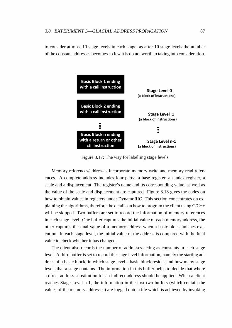
3.8. EXPERIMENT 5—GLACIAL ADDRESS PROPAGATION 87
to consider at most 10 stage levels in each stage, as after 10 stage levels the number
of the constant addresses becomes so few it is do not worth to taking into consideration.
Basic Block 1 ending
with a call instruction
Basic Block 2 ending
with a call instruction
Basic Block n ending
with a return or other
cti instruction
Stage Level 0 (a block of instructions)
Stage Level 1 (a block of instructions)
Stage Level n-1 (a block of instructions)
Figure 3.17: The way for labelling stage levels
Memory references/addresses incorporate memory write andmemory read refer-
ences. A complete address includes four parts: a base register, an index register, a
scale and a displacement. The register’s name and its corresponding value, as well as
the value of the scale and displacement are captured. Figure3.18 gives the codes on
how to obtain values in registers under DynamoRIO. This section concentrates on ex-
plaining the algorithms, therefore the details on how to program the client using C/C++
will be skipped. Two buffers are set to record the information of memory references
in each stage level. One buffer captures the initial value ofeach memory address, the
other captures the final value of a memory address when a basicblock finishes exe-
cution. In each stage level, the initial value of the addressis compared with the final
value to check whether it has changed.
The client also records the number of addresses acting as constants in each stage
level. A third buffer is set to record the stage level information, namely the starting ad-
dress of a basic block, in which stage level a basic block resides and how many stage
levels that a stage contains. The information in this bufferhelps to decide that where
a direct address substitution for an indirect address should be applied. When a client
reaches Stage Level n-1, the information in the first two buffers (which contain the
values of the memory addresses) are logged onto a file which isachieved by invoking

88 CHAPTER 3. DYNAMIC CODE ANALYSIS AND OPTIMIZATION
a thread for writing. When logging is finished, the two buffers are emptied and are
ready for recording the newly coming information. The information in the third buffer
is also processed and emptied every time a stage finishes execution. Moreover, a global
counter is set for each basic block to capture its repeated execution times. More fre-
quently executed basic blocks are better candidates for performing glacial addresses
replacement with constant addresses in the future work. Theinserted counter instruc-
tion cannot be only simply presented in the formatATOMIC_INC(counter),6 as simply
increasing the counter when the client sees a block will onlymake the client capture
the number of a specific basic block rather than its executionfrequency, therefore fre-
quency counter here will stay at one. As the client inserts instructions into each basic
block before its execution, this type of counter can only record the static number of the
basic blocks in a program rather than the dynamic number of times they are executed.
The way to capture the execution frequency of each block is toforce the frequency
counter to execute together with the application instructions. Figure 3.19 shows how.
The variablefreq_counteris the frequency counter.
dr_get_tls_field(dr_get_current_drcontext());dr_mcontext_t mc=sizeof(mc),DR_MC_ALL,;dr_get_mcontext(dr_get_current_drcontext(), &mc);base_reg_value=reg_get_value(temp_base,&mc);index_reg_value=reg_get_value(temp_index,&mc);
Figure 3.18: Codes to obtain the register value under DynamoRIO
instrlist_meta_preinsert(bb, instr,INSTR_CREATE_inc(drcontext, OPND_CREATE_ABSMEM((byte *)&(BufOne->freq_counter), OPSZ_4)));
Figure 3.19: Codes to obtain the execution frequency of eachblock under DynamoRIO
The results needed are the starting address of each basic block, the different num-
ber of stage levels that stages contain in a program, the address value information of
each stage level and the execution frequency of each basic block. Only results from
6 ATOMIC_INC increases the value of a variable by one; this is asafer way than counter++, as thevariable area will be locked while it increases thereby avoiding any concurrency problem.
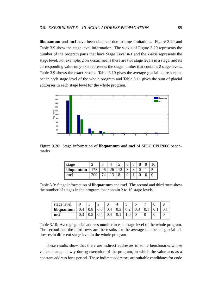
3.8. EXPERIMENT 5—GLACIAL ADDRESS PROPAGATION 89
libquantum and mcf have been obtained due to time limitations. Figure 3.20 and
Table 3.9 show the stage level information. The y-axis of Figure 3.20 represents the
number of the program parts that have Stage Level n-1 and the x-axis represents the
stage level. For example, 2 on x-axis means there are two stage levels in a stage, and its
corresponding value on y-axis represents the stage number that contains 2 stage levels.
Table 3.9 shows the exact results. Table 3.10 gives the average glacial address num-
ber in each stage level of the whole program and Table 3.11 gives the sum of glacial
addresses in each stage level for the whole program.
2 3 4 5 6 7 8 9 100
20
40
60
80
100
120
140
160
180
200
stag
e am
ount
libquantum
mcf
Figure 3.20: Stage information oflibquantum andmcf of SPEC CPU2006 bench-marks
stage 2 3 4 5 6 7 8 9 10libquantum 173 96 26 12 3 3 0 1 5mcf 200 74 13 8 0 1 0 0 0
Table 3.9: Stage information oflibquantum andmcf. The second and third rows showthe number of stages in the program that contain 2 to 10 stage levels
stage level 0 1 2 3 4 5 6 7 8 9libquantum 0.4 0.8 0.6 0.4 0.3 0.2 0.3 0.1 0.1 0.1mcf 0.3 0.5 0.4 0.4 0.1 1.0 0 0 0 0
Table 3.10: Average glacial address number in each stage level of the whole program.The second and the third rows are the results for the average number of glacial ad-dresses in different stage level in the whole program
These results show that there are indirect addresses in somebenchmarks whose
values change slowly during execution of the program, in which the value acts as a
constant address for a period. These indirect addresses aresuitable candidates for code

90 CHAPTER 3. DYNAMIC CODE ANALYSIS AND OPTIMIZATION
stage level 0 1 2 3 4 5 6 7 8 9libquantum 124 253 86 23 8 3 3 1 1 1mcf 77 141 37 9 1 1 0 0 0 0
Table 3.11: Sum of glacial addresses in each stage level of the program. The secondand the third rows are the results for the sum of the glacial addresses from Stage Level0 to Stage Level 9 of the whole program
replacement, which could enable a cascade of program optimization. For instance, ac-
cording to Table 3.10, the average number of glacial addresscandidates is 0.5 at Stage
Level One formcf. This means that the whole number of glacial address candidates on
Stage Level One can be significant in a program, as there are a large number of stages
in a program which incorporate a Stage Level One. As detecting glacial addresses in
a program is a dynamic procedure, a compiler is not able to perform such operations
due to lack of the online profile information.
3.8.2 Instrumentation Optimization
To accelerate the instrumentation speed, multiple threadsare generated by theGlacial-
Variable client to process the information in the buffers. There are two types of thread
under DynamoRIO: application thread and client thread. Anapplication threadworks
in DynamoRIO’s code cache. Aclient threadruns natively and does not execute its
code from the code cache. The application threads fill in the buffer with the target
profile information. The client threads process the profile information in the way de-
scribed in Section 3.8.1. Two sets of buffers are created. Each buffer set contains
two buffers: one for capturing the initial value of addresses and the other for captur-
ing the final value of the addresses. When the application under examination starts
execution, all the buffers are initialized and two clients threads are generated. The
application thread begins to fill in one set of the buffers. When this set of buffers is
full, the associated client thread begins to process them. Each client thread is bound to
one set of buffers. The client thread communicates with the application thread using
two associated semaphores, or to be more exact, the threads require a mutex to access
their associated buffer set. The application thread obtains the mutex for one associ-
ated buffer set and begins to fill in the profile information. While one stage finishes
execution, the application thread informs the appropriateclient thread that the buffer is
ready. The client thread then processes the set of buffers and meanwhile the applica-
tion thread fills in the profile information to the other available buffer set. Figure 3.21
3.8. EXPERIMENT 5—GLACIAL ADDRESS PROPAGATION 91
shows how to generate a client thread under DynamoRIO. The client thread will ter-
minate automatically when returning from the function or the whole program finishes
execution. The ways to generate and handle the client threads are similar to those of
POSIX threads.7
bool dr_create_client_thread(void (*func)(void *param), void *arg);
Figure 3.21: The DynamoRIO function8to generate a client thread
A signal (mutex) is triggered while the application thread finishes filling the pro-
file information of one block. To be more exact, the buffer only records the profile
information for one stage level. The signal handler performs two tasks. First the signal
handler signals the client thread to start processing the ready buffer by acquiring its
associated mutex. Next it switches to the next empty buffer set, returning when it has
successfully acquired one mutex. The buffer sets are switched by simply triggering a
signal (mutex). Figure 3.22 shows the multi-threading procedure.
7 POSIX thread manual: http://www.cs.nmsu.edu/ jcook/Tools/pthreads/pthreads.html.8 This instruction in this picture is a function declaration.

92 CHAPTER 3. DYNAMIC CODE ANALYSIS AND OPTIMIZATION
Due to time limitations, the performance improvement on benchmarks through pro-
cessing buffers by generating multiple threads have not been tested. This is reserved
for future work.
Initial final Initial final
Client
Thread1 App
Threads Client
Thread2
Buffer Set 1 Buffer Set 2
process process
input
Figure 3.22: Multi-threading procedure. Each client thread is bound to one bufferset. One buffer set contains two buffers. Client threads andapplications require theassociated mutex to access a buffer set
3.9 Chapter Summary
This chapter has presented some techniques for dynamic program analysis and op-
timization. Dynamic code analysis and optimization are performed as the program
executes. DynamoRIO is the platform used to perform runtimecode manipulation. By
defualt, any changes that are caused by runtime instrumentation do not reside in the
program when execution terminates. DynamoRIO works as an intermediate platform
between the application and the operating system. It introduces a large amount of run-
time overhead. The overhead can be offset by the performancegain of the program
when there is a large amount of code reuse. The runtime instrumentation is performed
by user-defined clients, which work together with DynamoRIOto perform the on-
line code analysis and optimization. DynamoRIO provides interfaces for user-defined
clients, so that the clients can take control and manipulatethe application instructions.
The SPEC CPU2006 benchmark suite is employed for testing theeffectiveness of the

3.9. CHAPTER SUMMARY 93
optimization techniques.
client name functionality
testremover remove redundanttestinstructionsadd2lea replaceaddwith lea where possiblenopremover removenopsnopoptimizer insertnopsCacheSimulator simulate cache miss and cache hitMemoryReference simulate memory reference changeBranchTarget simulate branch prediction changepersistcode perform persistent codeGlacialVariable: analyse the glacial variables in a program
Table 3.12: A list of all the implemented clients and their functionality
The clients that have been implemented and described in thischapter are summa-
rized in Table 3.12. Some of these clients have achieved the goals of dynamically re-
moving redundant instructions; strength reduction; instruction realignments; and anal-
ysis of the glacial addresses as the potential candidates for optimization. The imple-
mentation of clients under DynamoRIO has demonstrated the potential for dynamic
program optimization. However, this has not been always possible. Where it has been
possible, the performance results have been presented. Where not possible, an expla-
nation of the reasons has been given. For the program analysis only, results have been
presented to show the potential for code optimization in a program. The overall con-
clusion is that it is difficult to find performance gains that are large enough to offset the
cost of the dynamic analysis and code manipulation required. However, the results also
show that programs can in certain circumstances be made to run more quickly using
a variety of higher-level optimizations carried out at runtime, aided by observation of
control flow, data flow, and memory access patterns of applications as they run. There
is also a possibility to accelerate the program analysis by multi-threaded processing.
The next chapter turns to conclusions and discussion. It discusses the advantages
and disadvantages of the approaches presented in this chapter and evaluates the exper-
imental results. Future work is also proposed.

Chapter 4Conclusion and Discussion
94
Chapter 4
Conclusion and Discussion
4.1 Introduction
This chapter presents a summary of the thesis and its experimental results discussion,
which are covered in Section 4.2. Possible future work is proposed in Section 4.3.
4.2 Conclusion and Discussion
The thesis has presented some techniques for dynamic program analysis and optimiza-
tion. Five experiments have been carried out on a runtime code manipulation system
DynamoRIO. DynamoRIO works an intermediate platform between applications and
the operating system. DynamoRIO introduces a large amount of runtime overhead,
but this overhead can be offset by the performance gain of a program when there is a
large amount of code reuse. The runtime instrumentation is performed by user-defined
clients, which work together with DynamoRIO to perform online code analysis and
optimization. DynamoRIO provides interfaces for user-defined clients, so that such
clients can take control and manipulate the application instructions. Five experiments
are presented in the thesis. Some experiments have demonstrated program perfor-
mance improvement by runtime optimization. Where program improvement has not
been possible, an explanation has been given. The results for program analysis are also
presented to show the potential for other kinds of code optimization in a program.
In Section 3.4, removal of redundant instructions has been used in a static envi-
ronment in a previous publication. This thesis applies thisalgorithm in a dynamic
context. This has demonstrated performance improvement onsome benchmarks. Re-
dundant instruction identification and deletion is performed after the compiler applies
95

96 CHAPTER 4. CONCLUSION AND DISCUSSION
optimization on the program. Hence the performance of the developed method depends
on the compiler. The performance will differ when a different compiler is utilised.
Strength reduction, presented in Section 3.5, is an algorithm that could be utilised
on the runtime system which needs storing and restoring eflags during its context
switch. This approach could accelerate the program execution, however maybe a more
important usage of this method is to accelerate the online profile analysis when using
a runtime profile analysis tool. Benchmarkgcc fails during the testing. The reason
maybe thatgcc is more sensitive to flag fluctuation, there may be some trivial changes
of flags that leads the whole benchmark to crash. A verified reason for this at the time
of writing remains unknown.
Instruction alignment presented in Section 3.6 is a good example for architecture-
specific optimization that is better performed dynamically, tailoring the program to the
actual processor on which it is running on. This method has also been applied else-
where in a static context, but the thesis has shown that it maybe more worthwhile to
employ instruction alignment in a dynamic context to adjustthe layout of programs by
inserting or deletingnopsbased on their runtime behaviour. Therefore, three simula-
tors (memory reference simulator, branch target simulatorand cache simulator) have
been built to collect profile information of how program performance are affected by
insertingnops. However two simulators do not work well due to constraints in Dy-
namoRIO.
There is no deep investigation of persistent codes in Section 3.7, again constrained
by DynamoRIO itself. DyanmoRIO could only make the basic blocks persistent. A
large application is also not available for packing them as persistent codes. The results
show that the time of executing the persistent codes in the subsequent calls are slightly
shorter than the time of executing the code initially. This is because the subsequent
code is loaded directly without rebuilding basic blocks. The experiment in this thesis
is limited to enable persistent codes without any optimization algorithms applied in
them. Therefore, there is only a slight time difference between the initial execution
and a subsequent call. The benchmarks with little code reuseshow that there is execu-
tion time degradation in the following calls; however, it may be better to apply static
optimization on this type of program as building the persistent cache and restoring it
for the subsequent calls is also a time-consuming procedure.
Glacial address propagation, presented in Section 3.8, shows that there are indirect
addresses in programs whose values change sufficiently slowly in execution of the
program that it is worth generating special case codes, in which the address values are

4.3. FUTURE WORK 97
treated as constants for a period, thus enabling a cascade ofoptimization. However
the main focus of the approach in the thesis is on identification of the potential targets.
The large amount of runtime overhead caused by profiling and code replacement are
big obstacles that need to be overcome in future work.
The techniques presented in this thesis aim to optimize the program performance at
runtime. Since running a program faster can also be used to reduce the energy demand
of hardware, the presented optimization strategies can be applied as a way to optimize
hardware power consumption. Optimization of a program is a continuous procedure,
even when hardware is upgraded, yet the optimization strategies can improve the pro-
gram performance at a similar rate based on the new hardware.
4.3 Future Work
4.3.1 Integration of Static and Dynamic Optimization
The peephole optimizer developed by Sorav Bansal [8] is an outstanding static opti-
mizer, which optimizes the program offline. This static optimizer can automatically de-
tect and replace one sequence of instructions by another equivalent but faster sequence
of instructions. The peephole optimization could be performed before dynamic opti-
mization. The output from the peephole optimizer can be dumped into DynamoRIO
for further optimization.
DynamoRIO constructs the basic fragments, hashtable and other instrumentation
operations every time when importing a program even if the same program as before
is executed. When running a program with a large amount of code reuse, this overhead
can be offset by the performance gain. However, for a programwith little code reuse
or short execution time, the overhead caused by DynamoRIO initiation may not be
overcome by the program performance gain. To decrease this overhead, such a pro-
gram can be optimized in the initial execution and be constructed as persistent code
in a database. The optimized program will be loaded directlyfrom the database in the
subsequent calls. Figure 4.1 shows the possible infrastructure of the system described
above.
4.3.2 Glacial Addresses Optimization and Multiple Threading
Chapter 3 has presented the results for potential glacial indirect address candidates for
replacement with constant addresses. This work could be further extended to utilise

98 CHAPTER 4. CONCLUSION AND DISCUSSION
Figure 4.1: The infrastructure of the optimization system
such profile information to perform code replacement, thus enabling a cascade of op-
timization. This algorithm requires a large amount of time for profiling. In order to
reduce the online profiling overhead, multiple threads can be generated to process in-
formation. In Chapter 3, although parallel program analysis is implemented, no results
are presented to show its effectiveness on performance improvement which could be
completed in the proposed future work.
DynamoRIO provides a way to generate multiple client threads as well as synchro-
nisation primitives, such as mutex. However, at the time of writing, DynamoRIO does
not contain the functionality for conditional signals likethose in POSIX threads.1
More precisely, a thread cannot give a signal to another waiting thread when it fin-
ishes its job. The waiting thread has to keep checking its satisfied conditions all the
time. When the conditions are met, the waiting thread beginsto process or collect in-
formation. Threads will be suspended again when their working conditions cannot be
satisfied.
4.3.3 Memory Management
This thesis does not take memory management into account, asit only run one bench-
mark at a time. Memory control will not play an important roleuntil large applications
run or several applications run simultaneously. Memory expansion becomes a seri-
ous problem in the above situations. For instance, it can cause more cache misses
which reduce the benefits that come from code optimization. Also, in order to main-
tain execution of both application instructions and DyanmoRIO’s profile instructions,
1 POSIX thread manual: http://www.cs.nmsu.edu/ jcook/Tools/pthreads/pthreads.html.

4.3. FUTURE WORK 99
the memory requirement becomes much higher than for the original application alone.
Memory intensity analysis cannot only benefit the program performance but also
bring profits to the energy consumption of the computer system. Energy consumption
has been discussed in Section 4.3.5 and is widely felt to be critical for future systems.
Therefore memory usage management will be a promising area to be addressed in the
future work.
4.3.4 Possible Application Analysis
The thesis only covers performance analysis on benchmark suite SPEC CPU2006.
Industry is more interested in optimization approaches which can demonstrate per-
formance gain on real world, widely used applications. In order to achieve this, it
is possible to install the optimization system proposed in Section 4.3.1 in the operat-
ing system and make it work as a background application, therefore the optimization
system can automatically accelerate program execution andcontrol the application’s
memory expansion properly.
4.3.5 Energy Consumption Management
Power consumption and energy efficiency is becoming an increasingly important con-
cern for computer systems, especially for large computer systems and embedded sys-
tems [5]. Dynamic program optimization could lead to the acceleration of code genera-
tion and execution, which speed up program execution. Program optimization can also
lead to a fall in energy demand of the hardware. Software constitutes a major compo-
nent of systems and impacts the system power consumption. For instance, the choice
of algorithms, the layout of instruction sequences, the process of translating the high-
level codes into machine instructions and so on so forth, these procedures determine
the energy cost of software [42]. Limited by time, no investigation has been carried
out on the energy consumption fluctuation of the system due tosoftware optimization.
This could be carried out in future work.
To restrict control the energy demand to a low level, optimization on the program
is required not only to accelerate the program execution butalso to manage memory
intensity, cache intensity and CPU intensity. Evaluation tools are also needed in the
future research for estimating the power consumption of thehardware.
Energy consumption is a combined effect of various hardwarecomponents. There
are a few papers [27, 16] into energy estimation on analysingthe high-level input code

100 CHAPTER 4. CONCLUSION AND DISCUSSION
with the aid of information about hardware parameters, suchas the supply voltage, data
cache hit latency, memory access latencyet al. It is an open question how these energy
hints from program level can be exploited to benefit program optimization methodol-
ogy to reduce power consumption for hardware issues.

Bibliography
[1] IA-32 Intel architecture software developer’s manual,vol. 1-3. Order number
245470, 245471, 245472.
[2] Intel 64 and IA-32 Architectures Optimization Reference Manual.
[3] A. V. Aho and J. D.Ullman.Principles of Compiler Design. Addision-Wesley
Publication, 1977.
[4] T. Autrey and M. Wolfe. Initial results for glacial variable analysis.International
Journal of Parallel Programming, 26(1):43–64, Feb. 1998.
[5] W. Baek and T. M. Chilimbi. Green: a framework for supporting energy-
conscious programming using controlled approximation.ACM SIGPLAN No-
tices, 45(6):198–209, June 2010.
[6] V. Bala, E. Duesterwald, and S. Banerjia. Transparent dynamic optimization: The
design and implementation of dynamo. Technical report, HP Laborotory, 1999.
[7] V. Bala, E. Duesterwald, and S. Banerjia. Dynamo: a transparent dynamic opti-
mization system. InProceedings ACM SIGPLAN 2000 Conference on Program-
ming Language Design and Implementation, PLDI ’00, pages 1–12, New York,
NY, USA, 2000. ACM.
[8] S. Bansal and A. Aiken. Automatic generation of peepholesuperoptimizers. In
Proceedings 12th International Conference on Architectural Support for Pro-
gramming Languages and Operating Systems, ASPLOS-XII, pages 394–403,
New York, NY, USA, 2006. ACM.
[9] S. Bansal and A. Aiken. Binary translation using peephole superoptimizers. In
Proceedings 8th USENIX Conference on Operating Systems Design and Imple-
mentation, OSDI’08, pages 177–192, Berkeley, CA, USA, 2008. USENIX Asso-
ciation.
101

102 BIBLIOGRAPHY
[10] D. Bruening, E. Duesterwald, and S. Amarasinghe. Design and implementation
of a dynamic optimization framework for windows. In4th ACM Workshop on
Feedback-Directed and Dynamic Optimization (FDDO-4), 2000.
[11] D. Bruening, T. Garnett, and S. Amarasinghe. An infrastructure for adaptive
dynamic optimization. InInternational Symposium on Code Generation and Op-
timization, 2003. CGO 2003., pages 265 – 275, march 2003.
[12] D. Bruening and Q. Zhao. Practical memory checking withdr. memory. InPro-
ceedings 2011 9th Annual IEEE/ACM International Symposiumon Code Gener-
ation and Optimization (CGO), pages 213 –223, April 2011.
[13] D. L. Bruening. Eficient, Transparent, and Comprehensive Runtime Code Ma-
nipulation. PhD thesis, Massachusetts Institute of Technology, 2004.
[14] B. Calder and D. Grunwald. Fast accurate instruction fetch and branch prediction.
In 21st Annual International Symposium on Computer Architecture, pages 2–11.
ACM, 1994.
[15] W.-K. Chen, S. Lerner, R. Chaiken, and D. M. Gillies. Mojo: A dynamic op-
timization system. InProceedings ACM Workshop on Feedback-directed and
Dynamic Optimization (FDDO-3). ACM, 2000.
[16] M. Cohen, H. S. Zhu, S. E. Emgin, and Y. D. Liu. Energy types. In Object-
Oriented Programming, Systems, Languages, and Applications (OOPSLA’12),
2012.
[17] K. D. Cooper, M. W. Hall, and K. Kennedy. A methodology for procedure
cloning. Computer Languages, 19(2):105–117, Apr. 1993.
[18] R. G. D. Deaver and N. Rubin. Wiggins/restone: An on-line program specializer.
In Proceedings Hot Chips 11, August, 1999.
[19] E. Duesterwald and V. Bala. Software profiling for hot path prediction: less is
more.ACM SIGPLAN Notices, 35(11):202–211, Nov. 2000.
[20] A. C. S. B. Fl. and L. Carro.Dynamic Reconfigurable Architectures and Trans-
parent Optimization Techniques. Springer, 2010.

BIBLIOGRAPHY 103
[21] F. Gabbay and F. Gabbay. Speculative execution based onvalue prediction. Tech-
nical report, EE Department TR 1080, Technion - Israel Institue of Technology,
1996.
[22] F. Gabbay and A. Mendelson. Using value prediction to increase the power
of speculative execution hardware.ACM Transactions on Computer Systems,
16(3):234–270, Aug. 1998.
[23] R. Gupta, E. Mehofer, and Y. Zhang. Profile-guided compiler optimizations. In
Y. N. Srikant and P. Shankar, editors,The Compiler Design Handbook, pages
143–174. CRC Press, 2002.
[24] D. Hiniker, K. Hazelwood, and M. Smith. Improving region selection in dy-
namic optimization systems. InProceedings 38th Annual IEEE/ACM Interna-
tional Symposium on Microarchitecture, 2005. MICRO-38., pages 11 pp. –154,
Nov. 2005.
[25] R. Hundt, E. Raman, M. Thuresson, and N. Vachharajani. Mao - an extensi-
ble micro-architectural optimizer. In2011 9th Annual IEEE/ACM International
Symposium on Code Generation and Optimization (CGO), pages 1 –10, April
2011.
[26] H. Inoue, H. Hayashizaki, P. Wu, and T. Nakatani. A trace-based java jit compiler
retrofitted from a method-based compiler. InProceedings 9th Annual IEEE/ACM
International Symposium on Code Generation and Optimization, CGO ’11, pages
246–256, Washington, DC, USA, 2011. IEEE Computer Society.
[27] I. Kadayif, M. Kandemir, N. Vijaykrishnan, M. Irwin, and A. Sivasubramaniam.
Eac: a compiler framework for high-level energy estimationand optimization. In
Proceedings Design, Automation and Test in Europe Conference and Exhibition,
2002, pages 436 –442, 2002.
[28] V. Kiriansky, D. Bruening, and S. P. Amarasinghe. Secure execution via program
shepherding. InProceedings 11th USENIX Security Symposium, pages 191–206,
Berkeley, CA, USA, 2002. USENIX Association.
[29] J. L.Hennessy and D. A.Patterson.Computer Architecture-A Quantitative Ap-
proach. Elesevier,Inc, 2007.

104 BIBLIOGRAPHY
[30] M. H. Lipasti, C. B. Wilkerson, and J. P. Shen. Value locality and load value
prediction.ACM SIGPLAN Notices, 31(9):138–147, Sept. 1996.
[31] C.-K. Luk, R. Cohn, R. Muth, H. Patil, A. Klauser, G. Lowney, S. Wallace, V. J.
Reddi, and K. Hazelwood. Pin: building customized program analysis tools with
dynamic instrumentation. InProceedings 2005 ACM SIGPLAN Conference on
Programming Language Design and Implementation, PLDI ’05, pages 190–200,
New York, NY, USA, 2005. ACM Press.
[32] H. Massalin. Superoptimizer: a look at the smallest program. InProceedings 2nd
International Conference on Architectual Support for Programming Languages
and Operating Systems, ASPLOS II, pages 122–126, Los Alamitos, CA, USA,
1987. IEEE Computer Society Press.
[33] M. C. Merten, A. R. Trick, C. N. George, J. C. Gyllenhaal,and W.-m. W. Hwu.
A hardware-driven profiling scheme for identifying programhot spots to support
runtime optimization. InProceedings 26th Annual International Symposium on
Computer Architecture, ISCA ’99, pages 136–147, Washington, DC, USA, 1999.
IEEE Computer Society.
[34] N. Nethercote.Dynamic Binary Analysis and Instrumentation. PhD thesis, Com-
puter Laboratory, University of Cambridge, United Kingdom, Nov. 2004.
[35] K. Scott and J. Davidson. Strata: A software dynamic translation infrastructure.
Technical report, Charlottesville, VA, USA, 2001.
[36] J. Smith and R. Nair.Virtual Machines: Versatile Platforms for Systems and
Processes (The Morgan Kaufmann Series in Computer Architecture and Design).
Morgan Kaufmann Publishers Inc., San Francisco, CA, USA, 2005.
[37] A. Sodani and G. S. Sohi. An empirical analysis of instruction repetition.ACM
SIGOPS Operating System Review, 32(5):35–45, Oct. 1998.
[38] S. Sridhar, J. S. Shapiro, and P. P. Bungale. Hdtrans: a low-overhead dynamic
translator. ACM SIGARCH Computer Architecture News, 35(1):135–140, Mar.
2007.
[39] S. Sridhar, J. S. Shapiro, E. Northup, and P. P. Bungale.Hdtrans: an open source,
low-level dynamic instrumentation system. InProceedings 2nd International
BIBLIOGRAPHY 105
Conference on Virtual Execution Environments, VEE ’06, pages 175–185, New
York, NY, USA, 2006. ACM Press.
[40] T. Suganuma, T. Yasue, M. Kawahito, H. Komatsu, and T. Nakatani. Design and
evaluation of dynamic optimizations for a Java just-in-time compiler.ACM Trans-
actions on Programming Languages and Systems, 27(4):732–785, July 2005.
[41] T. Suganuma, T. Yasue, and T. Nakatani. A region-based compilation technique
for a Java just-in-time compiler.ACM SIGPLAN Notices, 38(5):312–323, May
2003.
[42] V. Tiwari, S. Malik, A. Wolfe, and M. T.-C. Lee. Instruction level power analysis
and optimization of software. InProceedings 9th International Conference on
VLSI Design: VLSI in Mobile Communication, VLSID ’96, page 326, Washing-
ton, DC, USA, 1996. IEEE Computer Society.
[43] M. N. Wegman and F. K. Zadeck. Constant propagation withcondi-
tional branches.ACM Transactions on Programming Languages and Systems
(TOPLAS), 13(2):181–210, Apr. 1991.
[44] Q. Zhao, I. Cutcutache, and W.-F. Wong. PiPA: pipelinedprofiling and analysis
on multi-core systems. InProceedings 6th Annual IEEE/ACM International Sym-
posium on Code Generation and Optimization, CGO ’08, pages 185–194, New
York, NY, USA, 2008. ACM Press.
[45] Q. Zhao, D. Koh, S. Raza, D. Bruening, W.-F. Wong, and S. Amarasinghe. Dy-
namic cache contention detection in multi-threaded applications.ACM SIGPLAN
Notices, 46(7):27–38, Mar. 2011.
[46] Q. Zhao, J. E. Sim, W. fai Wong, and L. Rudolph. DEP: detailed execution
profile. In Proceedings 15th International Conference on Parallel Architectures
and Compilation Techniques In PACT’06, pages 154–163. ACM Press, 2006.