dynamic pricing to improve supply chain...
TRANSCRIPT
Dynamic Pricing to improve Dynamic Pricing to improve Supply Chain PerformanceSupply Chain Performance
David Simchi-LeviM.I.T.
November 2000

Presentation OutlinePresentation Outline
• The Direct-to-Consumer Model– Motivation– Opportunities suggested by DTC
• Flexible Pricing Strategies• Future Research Directions

Characteristics of the Industrial PartnerCharacteristics of the Industrial Partner
• Make-to-stock environment• Annual revenue in 1998 was about $180 billion• Annual spending on supply is more than $70
billion• Huge product variety and a large number of
parts• Inventory levels of parts and unsold finished
goods is about $40 billion

RetailersDistribution
CenterManufacturer
Consumers
Direct to Consumer (DTC)Direct to Consumer (DTC)
The Impact of the DTC ModelThe Impact of the DTC Model
• Valuable Information for the Manufacturer – e.g., accurate consumer demand data

Traditional Supply ChainTraditional Supply Chain
Ord
er S
ize
Time
Source: Tom Mc Guffry, Electronic Commerce and Value Chain Management, 1998
CustomerDemand
CustomerDemand
Retailer OrdersRetailer OrdersDistributor OrdersDistributor Orders
Production PlanProduction Plan

The Dynamics of the Supply ChainThe Dynamics of the Supply Chain
Ord
er S
ize
Time
Source: Tom Mc Guffry, Electronic Commerce and Value Chain Management, 1998
CustomerDemand
CustomerDemand
Production PlanProduction Plan
We Conclude:We Conclude:
• Order Variability is amplified up the supply chain; upstream echelons face higher variability.
• What you see is not what they face.
In Traditional Supply Chains….
ConsequencesConsequences……..
• Increased safety stock
• Reduced service level
• Inefficient allocation of resources
• Increased transportation costs
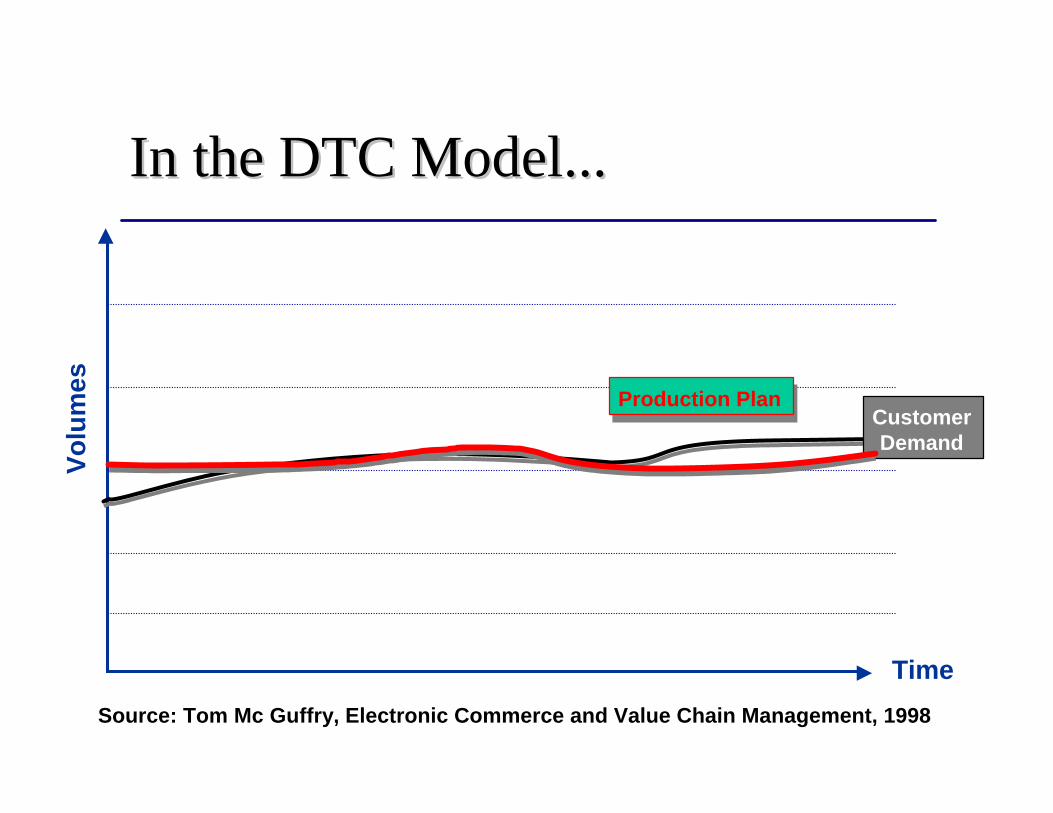
In the DTC Model...In the DTC Model...
Vo
lum
es
Time
Source: Tom Mc Guffry, Electronic Commerce and Value Chain Management, 1998
CustomerDemand
CustomerDemand
Production PlanProduction Plan

The Impact of the DTC ModelThe Impact of the DTC Model
• Valuable Information for the Manufacturer – e.g., accurate consumer demand data
• Product variety for the Consumer – e.g., allows for an assemble-to-order strategy

From MakeFrom Make--toto--Stock Model….Stock Model….
Suppliers Assembly Configuration

….to Assemble….to Assemble--toto--Order ModelOrder Model
Suppliers Assembly Configuration
A new Supply Chain ParadigmA new Supply Chain Paradigm
• A shift from a Push System...– Production decisions are based on forecast
• …to a Push-Pull System– Parts inventory is replenished based on
forecasts– Assembly is based on accurate customer
demand

The Impact of the DTC ModelThe Impact of the DTC Model
• Valuable information for the Manufacturer – e.g., accurate consumer demand data
• Product variety for the Consumer – e.g., allows for an assemble-to-order strategy
• Flexibility– e.g., price and promotions

Revenue ManagementRevenue Management
• “Allocating the right type of capacity to the right kind of customer at the right price so as to maximize revenue or yield”
• Traditional Industries: – Airlines– Hotels– Rental Car Agencies– Retail Industry
FOR EXAMPLE…
• McGill, J. and G. van Ryzin (1999), Revenue Management: Research Overview and Prospects. Transportation Science, 33, 2, pp. 233-256.

Traditional RequirementsTraditional Requirements
• Perishable inventory• Limited capacity• Ability to segment markets• Product sold in advance• Fluctuating demand
• Weatherford, L. and S. Bodily (1992), A Taxonomy and Research Overview of Perishable-Asset Revenue Management: Yield Management, Overbooking, and Pricing. Operations Research 40, 5, pp. 831-844.
FOR EXAMPLE…

Dynamic Pricing in ManufacturingDynamic Pricing in Manufacturing
• Non-perishable inventory• Production schedule needs to be determined• Production has capacity limitations• Demand and prices over time are bi-directional• Lost sales
FOR EXAMPLE…
• Federgruen, A. and A. Heching (1999), Combined Pricing and Inventory Control under Uncertainty. Operations Research, 47, 3,pp. 454-475.– Stochastic demand, allows for backlogging but not lost sales

Flexible Pricing in ManufacturingFlexible Pricing in Manufacturing
• Goals: – To extend the application of dynamic pricing and
revenue management to non-traditional areas• Manufacturing industry with non-perishable products• Capacity allocation is the allocation of a perishable resource
(i.e., build or no build decisions)
– To integrate pricing, production and distribution decisions within the supply chain
• “Allocate product to the right customer at the right price and at the right time”

Model FeaturesModel Features
• Determines “when” and “how much” to sell
• Capacity limitations on production• Incorporates lost sales• Known, time-dependent demand curves
Model AssumptionsModel Assumptions
• Deterministic model• Single product of discrete units• T periods• Periodically varying parameters:
– Production Capacity: Qt
– Holding Cost: ht per unit– Production Cost: kt per unit – Upper and lower bounds on price– Concave Revenue Function: Rt(Dt)
• Dt: the units of satisfied demand at period t• Example: Demand is a linear function of price

Revenue CurveRevenue Curve
Satisfied Demand
Revenue
• Revenue curve incorporates lost sales or limits on demand and remains concave with respect to satisfied demand
Price
CustomerDemand

The Pricing Problem: Problem PPThe Pricing Problem: Problem PP
Maximize Profit f(D) = ? 1<t<T (Rt(Dt) - ht It - kt Xt )Subject to:
(1) Beginning Inventory: I0 = 0(2) Inventory Balance: It = It-1 + Xt - Dt , t = 1,2,…,T(3) Production Capacity: Xt ? Qt, t = 1,2,…,T(4) Integrality: It , Xt, Dt, integer ? 0, t = 1,2,…,T
At each period t,– Xt is the units of product produced– It is the end of period inventory– Dt is the satisfied demand (sales)

When does flexible pricing When does flexible pricing matter?matter?• Computational analysis performed to
answer the following questions:– How much does flexible pricing affect profit?– When does flexible pricing have the most impact
on profit?– What other impacts does flexible pricing have?– How many prices in a horizon are needed to
obtain significant profit benefit?

Profit BenefitProfit Benefit
• Define profit potential due to flexible pricing to be:
• Profit potential is the percentage of profit to be gained from dynamic prices
1??PriceConstant h Profit witPrices Dynamich Profit wit
PotentialProfit
Computational DetailsComputational Details
• Demand curves obtained from an Industrial Partner
• Curves are aggregated over a number of products
• 10 period problem• Varied capacity, demand, or both

Managerial InsightsManagerial Insights
• Flexible pricing has the most impact on profit when:– Capacity is tightly constrained– Variability in capacity or demand
exists

Impact of Changes in CapacityImpact of Changes in Capacity• As capacity becomes more constrained, the benefit of flexible pricing increases• As the variability in capacity increases, the benefit of flexible pricing increases
Effect of Capacity Changes on Flexible Pricing Benefit when Demand is Constant
0%
5%
10%
15%
20%
25%
30%
0 0.1 0.2 0.3 0.4 0.5 0.6
Coefficient of Variation (Cap/Dem*)
% B
enef
it E(Cap/Dem*) = 0.5E(Cap/Dem*) = 0.75E(Cap/Dem*) = 1.0
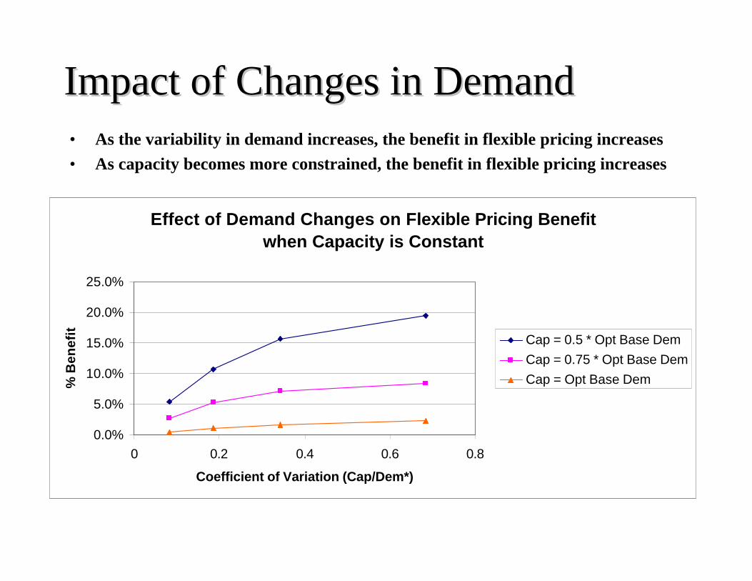
Impact of Changes in DemandImpact of Changes in Demand• As the variability in demand increases, the benefit in flexible pricing increases• As capacity becomes more constrained, the benefit in flexible pricing increases
Effect of Demand Changes on Flexible Pricing Benefit when Capacity is Constant
0.0%
5.0%
10.0%
15.0%
20.0%
25.0%
0 0.2 0.4 0.6 0.8
Coefficient of Variation (Cap/Dem*)
% B
enef
it
Cap = 0.5 * Opt Base DemCap = 0.75 * Opt Base DemCap = Opt Base Dem

Other Potential ImpactsOther Potential Impacts
• Reduction of variability in sales or production schedule
• Increase in average sales• Reduction of inventory• Reduction in average (or weighted
average) price

Impact on Variability of SalesImpact on Variability of Sales• When demand is variable and capacity is constant, flexible pricing
reduces the variability in sales compared to fixed pricing policies.
Effect of Pricing Policy on Variability of Sales when Capacity is Constant
0
0.1
0.2
0.3
0.4
0.5
0.6
0 0.05 0.1 0.15 0.2 0.25 0.3 0.35 0.4
Coefficient of Variation (Uncapacitated Demand)
Coe
ffic
ien
t of
Var
iati
on
(S
ati
sfie
d D
eman
d)
Flex Pricing: Cap = .75 Base D*
Fix Pricing: Cap = .75 Base D*
Flex Pricing: Cap = 1.0 Base Dem*
Fix Pricing: Cap = 1.0 Base Dem*

Impact on Production ScheduleImpact on Production Schedule• When demand is variable and capacity is constant, flexible pricing often results in
a smoother production schedule than that obtained using fixed pricing policies.
Effect of Pricing Policy on Variability of Production Schedule when Capacity is Constant
0
0.05
0.1
0.15
0.2
0.25
0.3
0.35
0.4
0 0.05 0.1 0.15 0.2 0.25 0.3 0.35 0.4
Coefficient of Variation (Uncapacitated Demand)
Co
effi
cien
t o
f V
aria
tio
n
(Pro
du
ctio
n) Flex Pricing: Cap = .75 Base D*
Fix Pricing: Cap = .75 Base D*
Flex Pricing: Cap = 1.0 Base Dem*
Fix Pricing: Cap = 1.0 Base Dem*

Impact on Average SalesImpact on Average Sales• Flexible pricing policies increase average sales compared to fixed
pricing policies.
Effect of Pricing Policy on Average Saleswhen Capacity is Constant
6000
7000
8000
9000
10000
11000
12000
0 0.05 0.1 0.15 0.2 0.25 0.3 0.35 0.4
Coefficient of Variation (Uncapacitated Demand)
Ave
rag
e S
atis
fied
Dem
and
Flex Pricing: Cap = .75 Base D*
Fix Pricing: Cap = .75 Base D*
Flex Pricing: Cap = 1.0 Base Dem*
Fix Pricing: Cap = 1.0 Base Dem*
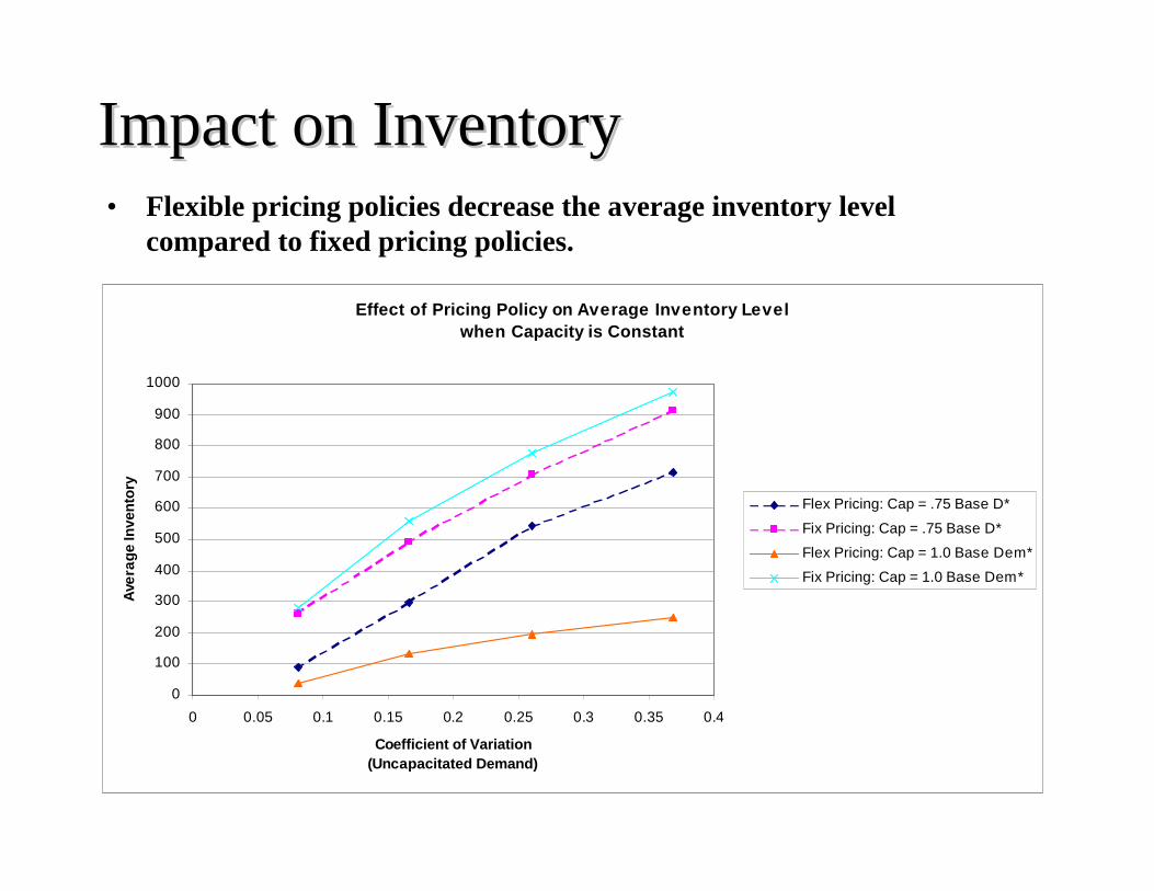
Impact on InventoryImpact on Inventory• Flexible pricing policies decrease the average inventory level
compared to fixed pricing policies.
Effect of Pricing Policy on Average Inventory Levelwhen Capacity is Constant
0
100
200
300
400
500
600
700
800
900
1000
0 0.05 0.1 0.15 0.2 0.25 0.3 0.35 0.4
Coefficient of Variation (Uncapacitated Demand)
Ave
rage
Inve
ntor
y
Flex Pricing: Cap = .75 Base D*
Fix Pricing: Cap = .75 Base D*
Flex Pricing: Cap = 1.0 Base Dem*
Fix Pricing: Cap = 1.0 Base Dem*

Impact on PriceImpact on Price• Flexible pricing policies decrease the weighted average price
compared to fixed pricing policies.
Effect of Pricing Policy on Weighted Average Price when Capacity is Constant
14000
15000
16000
17000
18000
19000
20000
0 0.05 0.1 0.15 0.2 0.25 0.3 0.35 0.4
Coefficient of Variation (Uncapacitated Demand)
We
igh
ted
Ave
rag
e (P
rice
)
Flex Pricing: Cap = .75 Base Dem*
Fix Pricing: Cap = .75 Base Dem*
Flex Pricing: Cap = 1.0 Base Dem*
Fix Pricing: Cap = 1.0 Base Dem*
Number of PricesNumber of Prices
• How many prices in a horizon are needed to obtain significant profit benefit?
• 12 periods analyzed– Considered 1, 2, 3, 4, 6, and 12 prices
• Test cases:– Varied capacity over the horizon, fixed demand curves– E(Capacity) = 0.50 * Optimal Uncapacitated Demand – For all patterns shown,
Coefficient of Variation (Capacity) = 0.25

Number of PricesNumber of Prices• Usually 1 price every 3 periods gives ? 75% of the potential profit increase• Less is sometimes more
Percentage of Potential Profit Increase due to Number of Prices
0.00%
20.00%
40.00%
60.00%
80.00%
100.00%
0 2 4 6 8 10 12
Number of Prices (out of 12)
% o
f Po
ten
tial
Pro
fit
Incr
ease
Pattern 1Pattern 2Pattern 3Pattern 4Pattern 5

Number of PricesNumber of Prices• Number of prices needed varies depending on the pattern of variability• The potential profit benefit varies depending on the pattern of variability
Increase in Profit due to Flexible Pricing Policies
0.0%
2.0%
4.0%
6.0%
8.0%
10.0%
12.0%
0 2 4 6 8 10 12
Num Price Changes (out of 12)
Pro
fit In
crea
se o
ver
Fix
ed
Pri
cing
Pattern 1
Pattern 2
Pattern 3
Pattern 4
Pattern 5
Multiple ProductsMultiple Products
• Deterministic multi-product model• Multiple products share common production capacity• Finite time horizon• Each product uses the same amount of the resource per
unit production• Time varying, product dependent parameters
– Production and inventory costs– Demand curves
Multiple Products: Computational ResultsMultiple Products: Computational Results
• 12 period horizon• Demand curves based on typical products• Demand Scenarios:
– Seasonality (car): low demand at beginning, increases in middle, decreases at end of horizon
– Decreasing Mean (laptop): demand steadily decreases from beginning to end of horizon
• Each product experiences the same seasonality effect

Profit Potential with Multiple ProductsProfit Potential with Multiple Products• The percentage of profit potential often decreases as the number of products
increases
Profit Potential with Multiple Products
0.0%
2.0%
4.0%
6.0%
8.0%
10.0%
12.0%
14.0%
16.0%
1 2 3 6 12 18
Number of Products
Pro
fit P
oten
tial
Seasonality (car)
DecMean (laptop)
Seasonality (car), high var
Future Research DirectionsFuture Research Directions
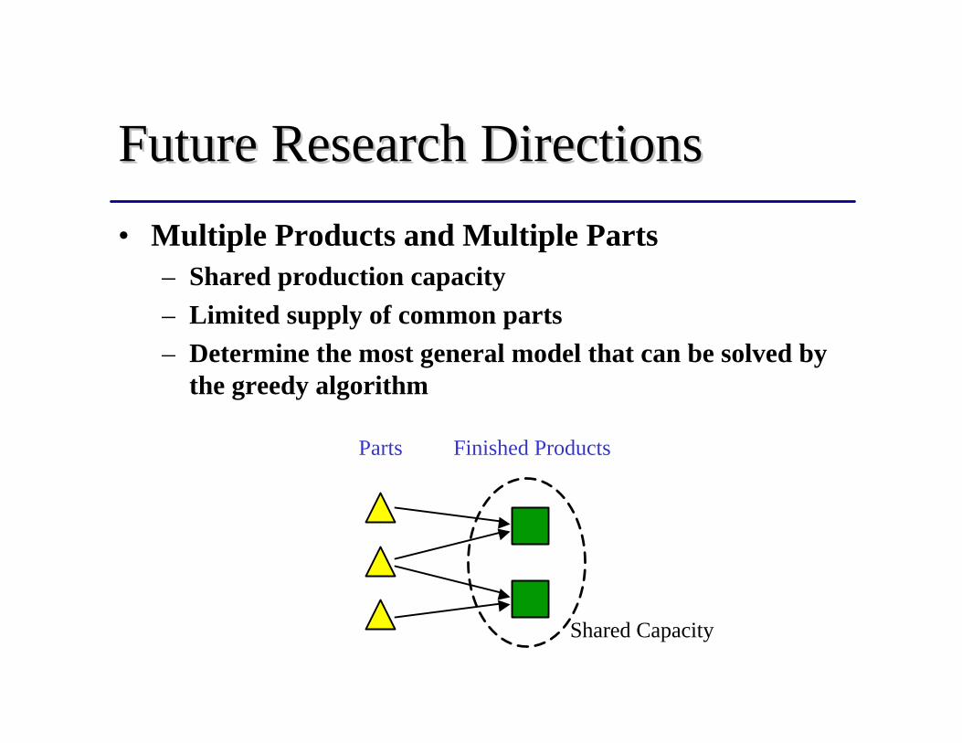
• Multiple Products and Multiple Parts– Shared production capacity– Limited supply of common parts– Determine the most general model that can be solved by
the greedy algorithm
Parts Finished Products
Shared Capacity
Future Research DirectionsFuture Research Directions
• Realistic Demand:– Stochastic Demand
• Computational analysis
– Demand Diversions• Price changes in one product influence customers to
divert from or to other products
• Production Set-up cost– Consecutive policy is optimal– DP that incorporates the MAA

Multiple Products, Part IIMultiple Products, Part II
• Stochastic Demand• Assumptions:
– Single period, n products– Production cost and salvage value– Products share limited production capacity– Demand for each product j is an r.v. with a known
cumulative probability distribution, FjP,D, which is
independent of the other products
• Goal: Set prices and production for all products to maximize expected profit
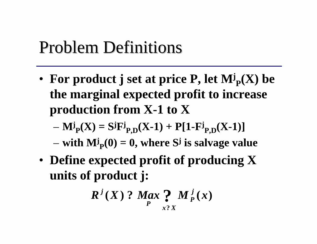
Problem DefinitionsProblem Definitions
• For product j set at price P, let MjP(X) be
the marginal expected profit to increase production from X-1 to X– Mj
P(X) = SjFjP,D(X-1) + P[1-Fj
P,D(X-1)]– with Mj
P(0) = 0, where Sj is salvage value
• Define expected profit of producing X units of product j:
??
?Xx
jPP
j xMMaxXR )()(

Problem FormulationProblem Formulation
• Problem PPE:– Max– Subject to
• Result:– If Rj(X) is a concave function of X for all j, then
problem PPE can be solved by MAA– Otherwise, PPE can be solved by a DP.
???
??nj
jjjjE XkXRXF1
))(()(
? ?j
j QX
njX j ,...,2,1,0 ?? integer
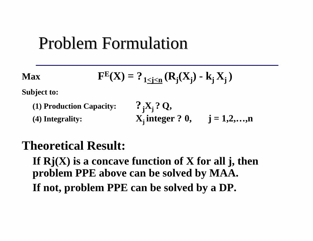
Problem FormulationProblem Formulation
Max FE(X) = ? 1<j<n (Rj(Xj) - kj Xj )Subject to:
(1) Production Capacity: ? jXj ? Q, (4) Integrality: Xj integer ? 0, j = 1,2,…,n
Theoretical Result:If Rj(X) is a concave function of X for all j, then problem PPE above can be solved by MAA.If not, problem PPE can be solved by a DP.
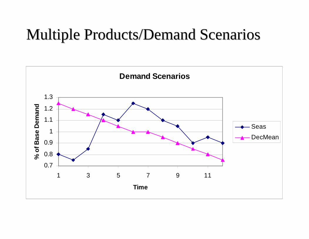
Multiple Products/Demand ScenariosMultiple Products/Demand Scenarios
Demand Scenarios
0.7
0.8
0.9
1
1.1
1.2
1.3
1 3 5 7 9 11
Time
% o
f Bas
e D
eman
d
Seas
DecMean