dynamic phasor based frequency scanning for grid-connected

Dynamic phasor based frequency scanning for grid-connected powerelectronic systems

M K DAS* and A M KULKARNI

Department of Electrical Engineering, Indian Institute of Technology Bombay, Mumbai 400076, India

e-mail: [email protected]; [email protected]

MS received 13 June 2015; revised 1 December 2016; accepted 31 January 2017; published online 11 October 2017

Abstract. Frequency scanning is a method of obtaining the frequency response of a system by injecting a

small-amplitude wide-band signal as an input in a time domain simulation of the system. This is an alternative to

analytical derivation of small-signal models, especially for complex grid-connected power electronic systems

(PESs). These models are required for the study of adverse interaction of PES with lightly damped oscillatory

modes in a power system. The use of the frequency scans for conventional small-signal stability analysis is

predicated upon the time-invariance of the underlying model. Since PES are generally time-periodic, time-

invariance may be achieved in some transformed variables. Although the DQ transformation is suitable in many

situations, it is not so for systems with low-order harmonics, individual-phase schemes, unbalanced or single-

phase systems, and PES with negative-sequence controllers. This paper proposes the use of dynamic phasor

variables in such situations since the underlying model in these variables is time-invariant. The procedure for

dynamic phasor based scanning is, however, intricate because wide-band signal injection results in the simul-

taneous presence of harmonic dynamic phasor components. The paper outlines this procedure and presents

illustrative case studies of Thyristor Controlled Series Compensator (TCSC) and STATCOM. For the TCSC, a

comparison of the frequency response obtained from the scanning method and the one obtained from an

approximate analytical dynamic phasor model is also presented.

Keywords. Frequency scanning; harmonic stability; impedance-based analysis; dynamic phasors; power-

electronics-based power system.

1. Introduction

Power electronic systems (PES) are increasingly being

deployed in power systems in the form of HVDC systems,

FACTS controllers and grid-interfaces for renewable

energy sources. These devices facilitate flexible operation

and control of power systems. Power electronic converters

generate harmonics and use fast-acting controllers, because

of which there is potential for adverse interactions with the

lightly damped oscillatory modes of the power system.

Adverse interactions can be manifested as harmonic mag-

nification [1], unstable torsional oscillations [2], or net-

work-controller mode instabilities [3].

Therefore, it is important to develop modelling and

analytical tools for the study of these adverse interactions in

grid-connected PES. One of the ways to analyse such

problems is the use of time-domain electro-magnetic tran-

sient simulations. Such simulations use detailed models of

PES. A large number of simulations are required for the

study of aspects like the effect of parameter variations and

the study of different contingencies. This is time-consum-

ing and the inferences may be case specific.

Analysis of the linearized state-space model of the

system can give a better insight into the effect of system

parameters. Tools like eigen-value analysis and Nyquist

criterion are useful for this purpose, but are applicable

only for Linear Time Invariant (LTI) systems. Dynamic

models for many PES may be developed by neglecting

harmonics and applying a time-variant DQ transformation

to the phase variables [4]. Alternative formulations based

on Dynamic Phasors [5] and Poincare-mapping based

discrete time models [6] have also been proposed. The

derivation of analytical models is tedious when the con-

verter, controllers and synchronization schemes have to be

represented accurately. An additional step of linearization

is also required, since most models are non-linear. Generic

models may not always be available, as many control

schemes of PES are not standardized. Modelling of

switching action in case of thyristor-based circuits is

complicated by the fact that turn-off instants are deter-

mined by the current through the devices. Therefore, rig-

orous analytical model development in a realistic situation

is often impractical.*For correspondence

1717

Sadhana Vol. 42, No. 10, October 2017, pp. 1717–1740 � Indian Academy of Sciences

DOI 10.1007/s12046-017-0701-1

http://crossmark.crossref.org/dialog/?doi=10.1007/s12046-017-0701-1&domain=pdf

http://crossmark.crossref.org/dialog/?doi=10.1007/s12046-017-0701-1&domain=pdf

Frequency scanning is a pragmatic alternative, which

involves the use of a time-domain simulation program to

numerically obtain the small-signal frequency response of a

system [7]. In this technique, a small-amplitude, wide-band

periodic signal is injected as an input in the time-domain

simulation of the system. The small-signal frequency

response of the system is obtained in the periodic steady

state, by computing the frequency components of the input

signal and the output variables. Examples of inputs and

outputs are current and voltage (to obtain the response of

the impedance), and generator speed and electrical torque

(to obtain synchronizing/damping torques). With this

approach, there are no restrictions on the extent of detail in

the system model. A user need not have the complete

details of the underlying model – the model is probed/

observed only at available inputs/outputs. Moreover, man-

ufacturers often provide highly accurate black-box simu-

lation models to their clients, and it is impossible to know

the details of the controllers. In such situations, a simula-

tion-based frequency scan is the only option.

The frequency response/transfer function concept is well

understood for systems. For such systems, further use of the

frequency response for stability analysis is also straight-

forward [8–11]. While small-signal injection ensures the

extraction of a linearized model, the time-invariance

property depends on the system model and the variables

used. Frequency scans obtained using variables in which

the model is time-variant are problematic, as they are dif-

ficult to interpret and utilize. For such systems, the fre-

quency response at one frequency may be distorted because

of the interference due to an injection at another frequency.

Fortunately, most PES are time-periodic systems.

Therefore, time-invariance may be achieved in some

transformed variables. Although the DQ transformation is

suitable when switching harmonics in the frequency range

of interest are negligible (e.g., a PWM-switched STAT-

COM analysed for low-frequency transients), this may not

be so for systems with low-order harmonics, systems using

individual-phase [12] or sequence-based controllers [13],

unbalanced systems [14] and single-phase systems. In such

situations, the use of dynamic phasor variables may yield

the desired time-invariance. Therefore they are the most

general variables for frequency scanning of PES. Dynamic

phasor based models are of infinite order (corresponding to

an infinite number of harmonic phasors), but a reduced

order is usually adequate for most applications.

The main contribution of this paper is to propose the use

of dynamic phasor variable based frequency scanning and

to present in detail, the methodology to obtain the same

using wide-band signal injection. Using the examples of

STATCOM and Thyristor Controlled Series Compensator

(TCSC), it is shown that for systems with negative-se-

quence controllers and low order harmonics, this scanning

yields a smooth frequency response that is independent of

the frequency content of the multi-sine input. This indicates

the underlying time-invariance of a dynamic phasor model.

For a TCSC, the frequency response obtained from a fre-

quency scan is compared with the one obtained from an

approximate analytical dynamic phasor model [5]. The

paper also presents the use of dynamic phasor model of

PES obtained by frequency scanning for grid interaction

studies.

The paper is organized as follows. In section 2, we

describe the existing techniques for frequency scanning

using phase, sequence and DQ variables and their limita-

tions. Section 3 describes the concept of Dynamic Phasors.

Section 4 presents the methodology for obtaining fre-

quency scans in these variables. Section 5 presents case

studies that illustrate the frequency responses of STAT-

COM and TCSC obtained using this method. Grid inter-

action studies using dynamic phasor models are described

in section 6.

2. The frequency scanning technique

In a time-domain simulation of a PES, a small-amplitude

voltage or current may be injected in order to get the fre-

quency response of admittance or impedance, respectively,

as shown in figure 1(a) and 1(b). This injection is super-

imposed upon the existing sources, which are required to

set up the equilibrium conditions around which the

response is obtained.

The injection of a sinusoidal voltage or current may be

done one frequency at a time. Each simulation has to be

carried out for a sufficient duration so that the natural

transients die out and the steady state is reached. This can

be time-consuming. Therefore, instead of obtaining the

steady state response for each frequency separately, a multi-

sine injection signal of the following form is generally

used:

uðtÞ ¼ aXN

l¼lo

sinð2pfd l t þ dlÞ: ð1Þ

All the frequency components of u(t) are multiples of fd.

Therefore, u(t) is periodic with a time period Td ¼ 1fd. Since

(a) (b)

Figure 1. Voltage- and current injection based frequency

scanning.

1718 M K Das and A M Kulkarni

fd is the interval between successive frequency components

of u(t), it indicates the resolution of the scan.

Since PES along with their controllers are generally non-

linear systems, the amplitude of u(t) must be small so that

the small signal frequency response of the linearized sys-

tem is obtained. Although ‘a’ itself could be chosen to be

very small, it may introduce errors due to finite precision.

Moreover, the remnant natural response of the system,

which never truly becomes zero in a finite duration, may

also become significant compared to the steady state

response due to u(t). This may cause distortions in the

frequency scan. Clearly, there is a trade-off among the

magnitude of a, duration of the scan and the accuracy of the

frequency response. For a given a, one can reduce the

overall amplitude of u by choosing dl to have a quadratic

dependence on l, as in the Schroeder multi-sine [15]:

dl ¼ �ðl � loÞðl � lo þ 1ÞðN � lo þ 1Þ p: ð2Þ

After the natural transients have (practically) died down, a

window of period Td is stored, and a Fast Fourier Trans-

form (FFT) [16] of both the input and output signals is done

in order to obtain the frequency response.

2.1 Scanning with phase/sequence variables

For three-phase systems, one may obtain the frequency

response by phase-wise injection (one phase at a time).

Alternatively, one may obtain the response in the sequence

variables, which are defined by the following

transformation.

xa

xb

xc

264

375 ¼

ffiffiffi1

3

r 1 1 1

e�j2p3 ej2p3 1

e�j4p3 ej4p

3 1

264

375

xþ

x�

xo

264

375: ð3Þ

The scheme for sequence-based scanning is shown in

figure 2. Sequence- or phase-based scanning is suitable for

passive time-invariant systems like capacitor/filter banks

and transmission lines.

Illustrative example: Sequence impedance model of a

distributed parameter transmission line. Consider a 500 kV

transmission line that is connected to voltage sources at

either end, with a 100 MVAr shunt reactor connected at its

midpoint—see figure 3. The transmission line is repre-

sented by the frequency-dependent phase model given in

PSCAD [17]. The tower configuration ‘Tower:3LVert’ of

PSCAD is used. The frequency responses of the network

impedances obtained by frequency scanning using

sequence variables are shown in figure 4. The multi-sine

parameters are a ¼ 1 kV and fd ¼ 1 Hz. The frequency

scanning range is from 1 Hz to 350 Hz. The given network

has a parallel resonance at 250 Hz. Non-zero coupling

terms in the frequency responses are present since the

Figure 2. Frequency Scanning based on sequence variables. Note that three scans are required, with different phase shifts.

Figure 3. The transmission network under consideration.

Dynamic phasor based frequency scanning 1719

conductors are placed in an unsymmetrical fashion on the

tower leading to sequence coupling.

2.2 Limitations of phase/sequence variable based

scans

Phase/sequence-based frequency scanning cannot be directly

used for PES that are time-variant when expressed in terms of

phase or sequence variables. As an example, consider a

±200 MVAr, STATCOM equipped with ‘Type-I’ con-

troller [4] as shown in figure 5. In the figure, the variables

shown with lower case subscripts ‘d’ and ‘q’ refer to the local

rotating frame, the reference for which is obtained by a PLL

tracking the STATCOM bus voltage v; ‘h’ is the output gen-erated by this PLL; vDC is the dc link voltage, whereas i rep-

resents the current. S�a, S�

b and S�c represent the modulating

signals used for PWM pulse generation.

The STATCOM is connected to a 500 kV, 50 Hz three-

phase voltage source through a 500 kV/25 kV converter

transformer. The STATCOM uses sine-triangle PWM to

generate firing pulses, with a carrier frequency of 1650 Hz.

For obtaining the frequency scan, a multi-sine voltage

signal, DvðtÞ, is injected as shown in figure 6(a), with

a ¼ 0:7 kV. The frequency scanning range is from 1 to

150 Hz with fd ¼ 1 Hz. The complete system is simulated

using PSCAD-EMTDC [17].

The frequency response of positive sequence admittance is

shown in figure 6(b). A distortion is seen in the frequency

range 1–100 Hz. This distortion can be explained as follows.

The model of a STATCOM in phase or sequence variables is

time-variant, involving multiplicative switching func-

tions [18], which have fundamental and harmonic compo-

nents. The injection of a positive sequence voltage at a

frequency x will cause negative and positive sequence cur-

rents at x� 2xo and x, respectively, due to the fundamental

component of the switching function. Moreover, if x\2xo,

then one would effectively have two positive sequence com-

ponents atx and 2xo � x due to sequence flipping [19]. The

latter can interferewith an additional positive sequenceoutput,

which will be present if there is a multi-sine injection com-

ponent at 2xo � x.This is also illustrated in figure 7 for the STATCOM, for a

single frequency injection at 20 Hz in positive sequence volt-

age. The 20 Hz signal causes positive sequence current com-

ponents at 20 and 80 Hz (�80 Hz in negative sequence) and no

negative sequence current in the positive frequency range.

Similarly, the injection of a negative sequence voltage at

a frequency x will cause positive and negative sequence

Figure 4. Frequency response of the transmission network.

Figure 5. STATCOM type-I controller [4].


currents at xþ 2xo and x, respectively, due to the fun-

damental component of the switching function. This is

illustrated in figure 8, for a single frequency injection of

negative sequence voltage at 20 Hz. In this case, there are

no additional frequency components in the positive and

negative sequence currents. A negative sequence scan,

therefore, does not have ‘interference’ (see figure 6(c)).

Distortions seen in frequency response of the positive

sequence admittance can be circumvented by limiting the

frequencies in a single scan (e.g. independent scans are

done from 0 to x0, x0 to 2x0 and so on) as shown in

figure 6(b). Although this gets rid of the interference, the

theoretical implications of the use of such scans for stability

analysis is unclear.

(a) (b)

(c)

Full scan, 1–150 Hz

, –

Figure 6. (a) Frequency scanning scheme for a STATCOM, (b) frequency response of positive sequence admittance and (c) frequencyresponse of negative sequence admittance.

(a) (b) (c)

Figure 7. Frequencies seen in the positive and negative sequence current when a positive sequence sinusoidal signal is injected at a

single frequency, 20 Hz.


2.3 Scanning with DQ variables

If switching is done in a balanced fashion and switching

harmonics are low, then the model of devices like a

STATCOM are time-invariant in DQ variables [4]. The DQ

transformation is defined as follows:

xa

xb

xc

264

375 ¼

ffiffiffi2

3

rcosðcÞ sinðcÞ 1ffiffiffi

2p

cos c� 2p3

� �sin c� 2p

3

� �1ffiffiffi2

p

cos c� 4p3

� �sin c� 4p

3

� �1ffiffiffi2

p

266666664

377777775

xD

xQ

xo

264

375

ð4Þ

c = xot, where xo is the operating frequency. The scheme of

DQ based injection [8] is shown in figure 9. Frequency

scanning set-up in PSCAD [17] is shown in figure 10 (Note

that any EMTP like software can be used for this purpose).

From PSCAD simulation, time-domain response of both

voltage and current in DQ variables are obtained. FFT oper-

ation in MATLAB [20] is used to extract frequency compo-

nents from these voltage and current responses.

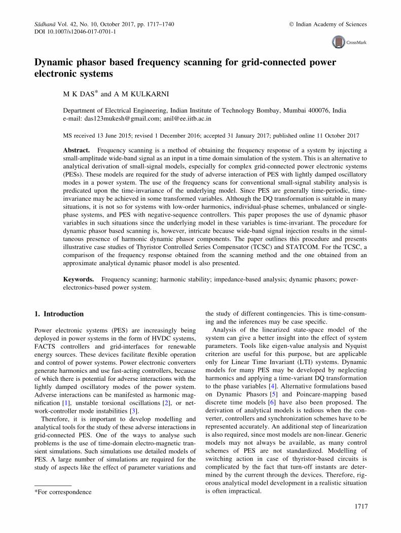
The frequency response of the DQ admittance model of the

STATCOM considered earlier is shown in figure 11. There is

no interference seen in the frequency scans due to the time-

invariance of the underlying model in the DQ variables. DQ-

based models are also time-invariant for balanced passive

systems and for balanced rotational machines [2].

2.4 Relationship between DQ model and sequence

model

The DQ admittance model is in the form of a matrix

transfer function as shown below:

(a) (b) (c)

Figure 8. Frequencies seen in the positive and negative sequence current when a negative sequence sinusoidal signal is injected at a

single frequency, 20 Hz.

Figure 9. Scheme based on DQ components. Three independent frequency scans are done: (1) by applying the multi-sine signal u(t) at

the point A keeping B and C at zero, (2) by applying u(t) at B, keeping A and C at zero and (3) by applying u(t) at C, keeping A and B at

zero.


Figure 10. Frequency scanning set-up in PSCAD.


IDðjxÞIQðjxÞ

� �¼

YDDðjxÞ YDQðjxÞYQDðjxÞ YQQðjxÞ

� �

|fflfflfflfflfflfflfflfflfflfflfflfflfflfflfflfflfflffl{zfflfflfflfflfflfflfflfflfflfflfflfflfflfflfflfflfflffl}YDQ

VDðjxÞVQðjxÞ

� �:

ð5Þ

Using (a) ejh ¼ cos hþ j sin h and (b) the frequency shift

property of the frequency response: XðjxÞ $ xðtÞ implies

Xðjx� jxoÞ $ ejxotxðtÞ, the DQ variables and sequence

variables can be related to each other in the frequency

domain by the following equation:

XDðjxÞXQðjxÞ

� �¼ 1ffiffiffi

2p

1 1

j � j

� �Xþðjxþ jxoÞX�ðjx� jxoÞ

� �: ð6Þ

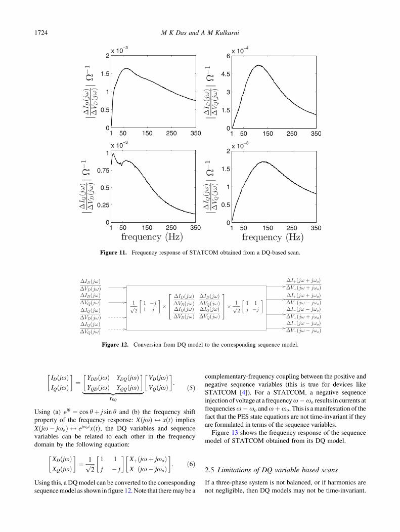
Using this, a DQmodel can be converted to the corresponding

sequencemodel as shown infigure 12.Note that theremaybe a

complementary-frequency coupling between the positive and

negative sequence variables (this is true for devices like

STATCOM [4]). For a STATCOM, a negative sequence

injection of voltage at a frequencyx� xo results in currents at

frequenciesx� xo andxþ xo. This is amanifestation of the

fact that the PES state equations are not time-invariant if they

are formulated in terms of the sequence variables.

Figure 13 shows the frequency response of the sequence

model of STATCOM obtained from its DQ model.

2.5 Limitations of DQ variable based scans

If a three-phase system is not balanced, or if harmonics are

not negligible, then DQ models may not be time-invariant.

Figure 11. Frequency response of STATCOM obtained from a DQ-based scan.

Figure 12. Conversion from DQ model to the corresponding sequence model.


In such cases, distortions in the frequency response may

result. This is illustrated using two examples.

2.5a Twelve-pulse STATCOM: PES like 12-pulse con-

verters and TCSC have significant lower order switching

harmonics. For a 12-pulse STATCOM, a significant

switching harmonic is present at 600 Hz (in the DQ

frame with fundamental frequency of 50 Hz). Thus a

sinusoidal injection at a frequency f will cause additional

components at 600� f . This is illustrated in figure 14, for

a single frequency injection of D-channel voltage at

340 Hz. Consequently, a scan using a multi-sine signal

having frequencies from 1 to 350 Hz will cause addi-

tional components at the sum and difference frequencies

(i.e. 250–600 Hz and 600–950 Hz). These additional

components between 250 and 600 Hz interact with the

frequency components between 250 and 350 Hz of the

wide-band signal and causes interference in the fre-

quency scan.

2.5b STATCOM with negative sequence controller: A

conventional STATCOM controller may be modified by

Figure 13. Frequency response of the sequence model of STATCOM obtained from its DQ-based scan.

(a) (b)

Figure 14. Twelve-pulse STATCOM: frequencies seen in the D-component of the current when the inject voltage DvD is a sinusoidal

signal at a single frequency, 20 Hz.


separating out the positive and negative sequence com-

ponents, and having separate controller channels to con-

trol these components individually [13]. This is a useful

feature for preventing unbalanced over-currents during

faults. The transient positive and negative sequence

components may be extracted by using notch-filters [21]

or time-delays [22]. The structure of the controller is

shown in figure 15, where the subscripts ‘?’ and ‘-’ refer

to the positive and negative sequence variables. The

implementation of the controller using positive and neg-

ative sequence components will lead to a time-variant

model in the DQ variables. Therefore, distortions are

expected in the DQ based frequency scans.

The frequency responses obtained from the DQ based fre-

quency scans (1–350 Hz) of a 12-pulse STATCOM and a

PWM-switched STATCOM that uses a sequence based

controller are shown in figure 16. The responses are not as

smooth as those in figure 11. As expected, there is a sig-

nificant distortion in the case of the 12-pulse STATCOM

above 250 Hz.

3. Dynamic phasors [5]

The kth Fourier coefficient or ‘‘Dynamic Phasor’’ hxik cor-

responding to a signal xðsÞ is defined as follows.

hxikðtÞ ¼1

T

Z t

t�T

xðsÞe�jkxosds ð7Þ

xðsÞ can then be represented in terms of complex Fourier

coefficients over a window length ‘T’ as follows:

xðsÞ ¼X1

k¼�1hxikðtÞejkx0s s 2 ½t � T ; tÞ ð8Þ

where xo ¼ 2pT. Usually, xo corresponds to the nominal

supply frequency in rad/s.

The important properties of dynamic phasors are as

follows.

(1) Derivative of the dynamic phasor is given by the

following equation.

Figure 15. STATCOM with a sequence based controller [21].

(a) (b)

Figure 16. Frequency response of (a) 12-pulse STATCOM and (b) STATCOM with a sequence-based controller, obtained from a DQ-

based scan.


dhxik

dt¼ dx

dt

�

k

�jkx0hxik: ð9Þ

This may be re-written as follows, by separating out the real

and imaginary terms.

dhxirek

dt¼ dx

dt

� re

k

þkx0hxiimk

dhxiimk

dt¼ dx

dt

� im

k

�kx0hxirek

ð10Þ

(2) The dynamic phasor of the product of two signals uðsÞand vðsÞ can be obtained by the discrete convolution of the

corresponding dynamic phasors as follows:

huvik ¼X1

l¼�1huik�lhvil ð11Þ

(3) If xðsÞ is real, then hxi�l ¼ hxi�lFor time-periodic systems, dynamic phasors are constant

in the steady state. The dynamic model of a system in

dynamic phasor variables, hxik, can be obtained from the

original model, which is in terms x, using (9) [5]. Equa-

tion (11) is useful if multiplicative switching functions

which are time-periodic in steady state are present in the

original model. The presence of these multiplicative terms

causes coupling between the dynamic phasors correspond-

ing to different k. The dynamic phasor models of time-

periodic PES are time-invariant and lend themselves easily

to conventional stability analysis [14].

3.1 Example of a dynamic phasor model

Consider a time-periodic system (with period T ¼ 2pxsÞ rep-

resented by the equation:

dxðtÞdt

¼ ð�10þ xs cosðxstÞÞxðtÞ: ð12Þ

The solution of this equation is given below,

xðtÞ ¼ eð�10tþsinðxstÞÞxð0Þ: ð13Þ

This solution can be checked by putting x(t) in Eq. (12).

The dynamic phasor model of the system given in (12) is

obtained using (9) as follows:

dhxik

dt¼ �ð10þ jkxsÞhxik þ xs

X1

l¼�1hcosðxstÞilhxðtÞik�l

¼ �ð10þ jkxsÞhxik þ xshcosðxstÞi1hxðtÞik�1

þ xshcosðxstÞi�1hxðtÞikþ1:

ð14Þ

There is a coupling between hxik, hxik�1 and hxikþ1. This

results in an infinite-dimensional state-space model. In

practice, a limited number of dynamic phasors are consid-

ered to model the system and the number of dynamic phasors

depends on the bandwidth of transient of interest. Consid-

ering real and imaginary parts of dynamic phasors as state-

variables, the state-space model is obtained as given in (15).

_hXi ¼ AhXi ð15Þ

where hXi is the state vector that consists of dc and real and

imaginary parts of dynamic phasors. The value of

hcosðxstÞi1 and hcosðxstÞi�1 are constant which results in

constant state matrix ‘A’. Hence, the developed dynamic

phasor model is time-invariant.

The solution of the dynamic phasor model is

hXiðtÞ ¼ eAðt�t0ÞhXiðt0Þ ð16Þ

where hXiðt0Þ is the value of all dynamic phasor compo-

nents at t ¼ t0.

3.1a Reconstruction of signal x(t) using dynamic pha-

sors: Reconstruction of x(t) using its dynamic phasors is

possible using following delayed reconstruction formula [23]:

xðsÞ ¼X1

k¼�1hxikðtÞejkx0s where s ¼ t� �; 0\�\T:

ð17Þ

Now we reconstruct x(t) from its dynamic phasors and the

accuracy of reconstruction is checked with the exact solu-

tion of x(t) as given in (13). Three different values of � ¼ T,

T/2 and T/4 are used. For initial condition, t0 ¼ T is con-

sidered and hXiðTÞ is numerically evaluated from the actual

response of x(t) using (7): hxi0ðTÞ ¼ 1:1796, hxire1 ðTÞ ¼

0:0087, hxiim1 ðTÞ ¼ �0:5512, hxire

2 ðTÞ ¼ �0:1344,

hxiim2 ðTÞ ¼ �0:0177, hxire

3 ðTÞ ¼ �0:0042, hxiim3 ðTÞ ¼

0:0126 and so on.

3.1b Case 1: k ¼ �1 and 0: The dynamic phasor model is

obtained considering fundamental and DC dynamic phasor

(other dynamic phasors are neglected) using (14) as

follows:

d

dt

hxi0hxire

1

hxiim1

2

64

3

75 ¼�10 xs 0

0:5xs �10 xs

0 �xs �10

2

64

3

75hxi0hxire

1

hxiim1

2

64

3

75: ð18Þ

Eigen-values of this system are �10 and �10� j222:14.The solution of the dynamic phasors is obtained using (16).

Signal x(t) is reconstructed using (17) with different values

of � and shown in figure 17. There is an error in the

reconstructed signal and the exact signal. Note that for � ¼T ; T=2 and T / 4, the reconstructed signal is obtained from

t ¼ 0, t ¼ T=2 and 3T4, respectively.

Case 2: k ¼ �3;�2;�1 and 0 The dynamic phasor model

is given below:


The eigen-values of the above system are �10� j313:67,�10� j643:45, �10� j849:28 and �10. Similarly signal is

reconstructed using dynamic phasors and shown in fig-

ure 18. There is a close match between the reconstructed

signal and exact solution of x(t) for � ¼ T=2 and T/ 4.

Similarly, the eigen-values obtained by considering

dynamic phasors of k ¼ 5; 4; 3; 2; 1 and 0 are

�10� j314:16, �10� j628:33, �10� j941:99,�10� j1271:8, �10� j1477:6 and �10.

Remarks

1. Reconstruction with � ¼ T gives inaccurate results even

if many dynamic phasors are considered.

2. With �\T , the reconstruction becomes more accurate as

k is increased.

3. The low-frequency eigen-values of the dynamic phasor

model seem to converge as k is increased.

4. The dynamic phasor model shows that the system is

stable. This is consistent with the actual system

response.

4. Dynamic phasor based frequency scanningprocedure

In the extraction of the frequency response in the dynamic

phasor variables we encounter several issues that are not

encountered in phase/sequence or DQ based scanning.

These issues are discussed here.

(1) Theoretically, there are infinite dynamic phasors

(k ¼ �1 to 1) for a signal injected or observed in the

time-domain simulation of the system. For practical sys-

tems, consideration of a limited number of dynamic phasors

is usually adequate for stability analysis.

For a single-phase system, even if a few phasors are

considered, say (k ¼ 0; 1), then the admittance is in the

form of a matrix transfer function as follows:

hDIi0ðjxÞhDIire

1 ðjxÞhDIiim

1 ðjxÞ

2

64

3

75 ¼G11 G12 G13

G21 G22 G23

G31 G32 G33

2

64

3

75hDVi0ðjxÞhDVire

1 ðjxÞhDViim

1 ðjxÞ

2

64

3

75:

ð20Þ

Notation: hDIire1 ðjxÞ is the frequency domain representa-

tion of hDiire1 , which is the real part of the dynamic phasor

of DiðtÞ. hDIiim1 ðjxÞ is the frequency domain representation

of hDiiim1 , which is the imaginary part of the dynamic

phasor of DiðtÞ. Note that both hDiire1 and hDiiim

1 are real

signals, whereas hDIire1 ðjxÞ and hDIiim

1 ðjxÞ are complex

numbers.

Since the time-domain simulation model is generally not

in dynamic phasor variables, we have to use a discrete-time

approximation of (7) to evaluate hDiik and hDvik from DiðtÞ

Figure 17. Plot of time domain signal, x(t) for exact and dynamic

phasor (k ¼ 1 and 0) solutions.

0 0.02 0.04 0.06 0.08 0.1 0.12 0.150

0.5

1

1.5

2

2.5

Figure 18. Plot of time domain signal x(t) for exact and dynamic

phasor (k ¼ 3; 2; 1 and 0) solutions (responses with � ¼ T=2 and

T / 4 completely overlapped with the actual response).

d

dt

hxi0hxire

1

hxiim1

hxire2

hxiim2

hxire3

hxiim3

2

666666666664

3

777777777775

¼

�10 xs 0 0 0 0 0

0:5xs �10 xs 0:5xs 0 0 0

0 �xs �10 0 0:5xs 0 0

0 0:5xs 0 �10 2xs 0:5xs 0

0 0 0:5xs �2xs �10 0 0:5xs

0 0 0 0:5xs 0 �10 3xs

0 0 0 0 0:5xs �3xs �10

2

666666666664

3

777777777775

hxi0hxire

1

hxiim1

hxire2

hxiim2

hxire3

hxiim3

2

666666666664

3

777777777775

: ð19Þ


and DvðtÞ, respectively. FFT algorithm is then used to

obtain hDIirek ðjxÞ, hDIiim

k ðjxÞ, hDVirek ðjxÞ and hDViim

k ðjxÞ.(2) It is not possible to exclusively inject one dynamic

phasor at a time. If the input signal isuðtÞ ¼ ejxit , then in terms

of dynamic phasor variables, it implies a simultaneous injec-

tion of hui0 at the frequency xi, hui1 ¼ huire1 þ jhuiim

1 at

xi � xo, hui2 ¼ huire2 þ jhuiim

2 at xi � 2xo, and so on.

If the underlying system is time-invariant in the dynamic

phasor variables, then the dynamic phasor of the output

signal y(t) will contain these frequencies as well. Moreover,

one can attribute all the output dynamic phasors at the

frequency xi to the input hui0, the dynamic phasors at the

frequency xi � xo to the input hui1 and so on.

In other words, an injection of u(t) at the frequencyxi will

yield the following frequency responses in the steady state:

hYi0ðsÞhUi0ðsÞ

;hYi1ðsÞhUi0ðsÞ

;hYi2ðsÞhUi0ðsÞ

; :::: at s ¼ jxi

hYi0ðsÞhUi1ðsÞ

;hYi1ðsÞhUi1ðsÞ

;hYi2ðsÞhUi1ðsÞ

; :::: at s ¼ jðxi � x0Þ

hYi0ðsÞhUi2ðsÞ

;hYi1ðsÞhUi2ðsÞ

;hYi2ðsÞhUi2ðsÞ

; :::: at s ¼ jðxi � 2x0Þ

::::

::::

hYi0ðsÞhUinðsÞ

;hYi1ðsÞhUinðsÞ

;hYi2ðsÞhUinðsÞ

; :::: at s ¼jðxi � nx0Þ:

Similarly, for the input uðtÞ ¼ e�jxi t,

hYi0ðsÞhUi0ðsÞ

;hYi1ðsÞhUi0ðsÞ

;hYi2ðsÞhUi0ðsÞ

; :::: at s ¼� jxi

hYi0ðsÞhUi1ðsÞ

;hYi1ðsÞhUi1ðsÞ

;hYi2ðsÞhUi1ðsÞ

; :::: at s ¼� jðxi þ x0Þ

hYi0ðsÞhUi2ðsÞ

;hYi1ðsÞhUi2ðsÞ

;hYi2ðsÞhUi2ðsÞ

; :::: at s ¼� jðxi þ 2x0Þ

::::

::::

hYi0ðsÞhUinðsÞ

;hYi1ðsÞhUinðsÞ

;hYi2ðsÞhUinðsÞ

; :::: at s ¼� jðxi þ nx0Þ:

Note that for k 6¼ 0,

hUikðsÞ ¼hUirek ðsÞ þ jhUiim

k ðsÞhYikðsÞ ¼hYire

k ðsÞ þ jhYiimk ðsÞ:

Since the real and imaginary components of input and

output dynamic phasors are real signals

hUirek ðjxiÞ ¼ hUire

k�ð�jxiÞ; hUiim

k ðjxiÞ ¼ hUiimk

�ð�jxiÞhYire

k ðjxiÞ ¼ hYirek�ð�jxiÞ; hYiim

k ðjxiÞ ¼ hYiimk

�ð�jxiÞ

where ‘�’ represents the complex conjugate operation. To

obtain the frequency responses of individual real and

imaginary components, we can use the following

relationships.

If M ¼ hYikðjxÞhUimðjxÞ

and N ¼ hYikð�jxÞhUimð�jxÞ then

hYirek ðjxÞ

hYiimk ðjxÞ

" #¼

1 j

1 �j

� ��1M jM

N� �jN�

� � hUirem ðjxÞ

hUiimm ðjxÞ

" #:

ð21Þ

Although the analysis presented so far uses complex input

signals ejxi t and e�jxit, actual injection is in terms of real

sinusoidal and cosinusoidal (i.e., phase shifted by p2) signals,

from which we can obtain the required responses, using the

well known relationships between these functions.

(3) If all components of the matrix transfer function

corresponding to the dynamic phasors from k ¼ 0 to n in a

frequency range 0–xmax are desired, then xi of the input

signal has to be varied from 0 to (xmax þ nx0).

(4) If a multi-sine signal is injected, then it is important to

avoid overlap of frequencies in order to correctly identify all

transfer functions. Therefore, to obtain the frequency response

from, say, 0 to 3xo, we need to carry out three scans: (i) from0

toxo, (ii) fromxo to 2xo and (iii) from 2xo to 3xo. For three-

phase systems, the injection will have to be done one phase or

one sequence component at a time. It is not possible to obtain

the frequency response at the exact multiples of the funda-

mental frequency, as dynamic phasor components at these

frequencies cannot be recovered (they are zero). Therefore,

one may infer these by interpolation.

The complete procedure for scanning based on dynamic

phasor variables is depicted in figure 19.

Complexities involved in the dynamic phasor based fre-

quency scanning as illustrated using the example of a 12-pulse

STATCOM. A sinusoidal signal uðtÞ ¼ sinð2 p 20 tÞ at a sin-gle frequency of 20 Hz is injected in the phase ‘a’ of the

STATCOM (no injection in phase ‘b’ and ‘c’). The frequency

components present in the dynamic phasor components of

input voltage are shown in figure 20. As expected, the 20-Hz

component is present in hDVai0, 30 and 70 Hz components are

present hDVai1, 80 and 120 Hz are present in hDVai2 and 130and 170 Hz are present in hDVai3.

The dynamic phasors extracted using output currents are

shown in figure 20. In hDIai0, the frequency component at

20 Hz is generated due to the input hDVai0 and 80 and

120 Hz components are generated due to hDVai2. Similarly,

the presence of different frequency components present in

the other current dynamic phasors can be explained.

5. Examples of dynamic phasor based scanning

5.1 TCSC

Consider a TCSC connected to a 50 Hz current source as

shown in figure 21(a). The parameters of the TCSC are as


follows [24]: L ¼ 12:4 mH, C ¼ 82 lF, and the rms value

of the current source is 1 kA. The TCSC operates at a

firing delay angle of 63�. The firing pulses are generated

with respect to the positive zero crossing of the line

current.

To obtain the frequency scan, a multi-sine current Di is

injected as shown in figure 21(a). Note that the simulation

includes the switching action of the thyristors and the firing

angle synchronization with the line current. The multi-sine

parameters are a = 0.001 kA and fd = 1 Hz. The frequency

scanning range is from 1 to 200 Hz.

Figure 19. Frequency scanning technique using dynamic phasor variables.

cFigure 20. Frequencies seen in the dynamic phasor components

of the voltage of phase ‘a’ when a sinusoidal voltage uðtÞ ¼sinð2 p 20 tÞ which contains a single frequency, 20 Hz, is injected

in phase ‘a’ of a 12-pulse STATCOM.


(a) (b)

(c) (d)

(e) (f)

(g) (h)

(i) (j)


The frequency response of the TCSC using different

multi-sine signals is shown in figure 21. Multi-sine-1

uses Schroeder’s multi-sine signal—see Eq. (2). Multi-

sine-2 is generated by minimizing the overall magni-

tude of u(t) (1) in the selected frequency range using a

genetic algorithm based optimization tool in

MATLAB [20]. The resulting frequency response

shows distortions from 100 Hz to 200 Hz as shown in

figure 21. The switching harmonic at 300 Hz (in the

DQ frame) multiplicatively interacts with the frequency

components between 100 and 200 Hz of the wide-band

signal, to cause additional interfering components

between 100 and 200 Hz. This is also illustrated in

figure 22, for a single frequency injection at 20 Hz in

the input D-channel. The 20-Hz signal interacts with

the 300-Hz switching harmonic to cause components at

280 Hz and 320 Hz. If two independent scans are

carried out (0–150 Hz and 150–200 Hz), then the

additional components in each scan fall outside the

interval of that scan, and are easy to identify and

discard. This results in a smoother overall scan, as

shown in figure 21. The scans have significant differ-

ences in the higher frequency range, which is

indicative of the time-invariance of the system in the

DQ variables due to the low order harmonics.

In the following sub-section, we obtain the dynamic

phasor scans using the procedure presented in the previous

section, and also compare them with those obtained using

an approximate analytical model.

5.1a Approximate analytical model of a TCSC: The state

equations representing TCSC (for one phase) are given by

the following equations:

Ldi

dt¼ qvc

Cdvc

dt¼ iL � i

ð22Þ

where iL represents the line current; vc and i denote the

voltage across the capacitor and the current through the

inductor, respectively; ‘q’ is the switching function which

depends on the thyristor states i.e., if a thyristor is on,

q ¼ 1, and q ¼ 0 when a thyristor is off.

Using (9) and (10), the equations given in (22) are

rewritten in terms of the dynamic phasors. The equations

for the kth dynamic phasor are as follows:

(a) (b)

Figure 21. (a) Frequency scanning set-up for a TCSC and (b) frequency response of TCSC obtained by DQ based scanning (Quiescent

delay angle, a0 ¼ 156o).

(a) (b)

Figure 22. TCSC: frequencies seen in the D-component of the voltage when the inject current, DiD is a sinusoidal signal at a single

frequency, 20 Hz.


Ldhiire

k

dt¼ kx0hiiim

k þ hqvcirek

Ldhiiim

k

dt¼ �kx0hiire

k þ hqvciimk

Cdhvcire

k

dt¼ kx0hvciim

k þ hiLirek � hiire

k

Cdhvciim

k

dt¼ �kx0hvcire

k þ hiLiimk � hiiim

k :

ð23Þ

The term hqvcik creates a coupling between dynamic pha-

sors corresponding to different values of k as a result of

(11).

Since the turn-off instants of the thyristors are dependent

on the circuit conditions, switching function ‘q’ may be

obtained by iteratively solving transcendental equa-

tions [25], which makes the model complicated. In [5]

and [25], it is assumed that the peak of the actual inductor

current is symmetrical about its fundamental component,

and k is restricted to 1, 3 and 5. Since low-frequency

transients are of interest, the differential equations corre-

sponding to hiik are converted to algebraic equations by

replacing the derivative of hiik with zero. This results in an

approximate low-frequency model having six states per

phase for a constant firing angle delay. This model is lin-

earized and the frequency responses may be obtained

analytically.

5.1b Comparison of the frequency responses: The

dynamic phasor based impedance obtained from the

Figure 23. Frequency response of TCSC (dynamic phasor based) for one phase obtained analytically and by frequency scanning.


analytical model and the one obtained from the simula-

tion based scan is shown in figure 23. Only a few transfer

function components are shown. At low frequencies both

the responses are identical but are significantly different

at high frequencies. This is expected, as the analytical

model is an approximate one and is valid only at low

frequencies. Note that the dynamic phasor scans are

much smoother compared to the DQ based scan shown in

figure 21.

5.2 STATCOM

Dynamic phasor based scanning of the 12-pulse STAT-

COM and the PWM-switched STATCOM with a sequence

controller (considered in section 2) is carried out. The

multi-sine parameters are same as used earlier in the DQ

based scan.

The frequency response of some of the elements of

admittance matrix (in terms of sequence components of the

dynamic phasors) is shown in figures 24 and 25. The

responses are smooth, indicating the time invariance

property of the underlying model in dynamic phasor

variables.

Table 1 presents different systems encountered in prac-

tice and the nature of various models. A time-domain signal

x(t) and its kth dynamic phasor hxikðtÞ are related in fre-

quency domain as follows: hXikðsÞ ¼ 1T

ð1�e�sT Þs

Xðs þ jkxoÞ.

6. Grid interaction studies using dynamic phasorfrequency scans

Small-signal instabilities may occur due to adverse inter-

actions between a grid and a connected PES. The main use

of frequency scanning is the study of such adverse inter-

actions. For this, the complete system is represented as the

combination of two independent systems as shown in fig-

ure 26, while the closed-loop frequency response of the

system may be obtained as shown in figure 26. The closed-

loop transfer function is ZeqðjxÞ ¼ ðZGRIDðjxÞ�1þYPESðjxÞÞ�1

. ZGRIDðjxÞ and YPESðjxÞ are the impedance

and admittance matrices of the grid and PES respectively1,

the latter being obtained using frequency scanning, while

the former may be obtained using an analytical model or by

frequency scanning. Closed-loop Nyquist Criterion may be

used to check the stability of this closed-loop system pro-

vided both the model of Grid and PES are LTI.

In both DQ and Dynamic Phasor based analyses, ZGRID

and YPES are matrix transfer functions. Therefore, the

generalized Nyquist Criterion (GNC) is used to check the

stability of the closed-loop feedback system.

Figure 24. Frequency response obtained from a dynamic phasor based scan of a 12-pulse STATCOM.

1For devices like TCSC, the dual form is used with ZPES and YGRID.


Figure 25. Frequency response obtained from a dynamic phasor based scan of a PWM-switched STATCOM with a sequence based

controller.

Table 1. Inter-convertibility among phase/sequence, DQ and dynamic phasor model for different type of systems (NA: not-applicable).

System Example

Phase/

sequence

model

DQ

model

Dynamic phasor

model in phase/

sequence variables Remark

No switching elements

Three-phase balanced system Balanced inductor and

capacitor banks,

transmission lines

LTI

(diagonal)

LTI LTI (block

diagonal)

Models are completely inter-

convertible

Three-phase unbalanced system Unbalanced inductor

and capacitor

banks,transmission

line

LTI

(sequence

coupling)

Not

LTI

LTI (block

diagonal)

Phase model and dynamic

phasor model are inter-

convertible

Single-phase Single pahse inductor,

capacitor,

transmission line

LTI NA LTI (block

diagonal)

Phase model and dynamic

phasor model are inter-

convertible

With switching elements

Single-phase converter Single phase rectifier,

inverter

Not LTI NA LTI

Balanced three- phase converter

with negligible harmonics in

switching function

PWM switched

STATCOM

Not LTI LTI LTI DQ to phase model (at

complementary

frequencies) is possible

Balanced three-phase converter

with significant harmonics in

switching function

12-pulse STATCOM,

TCSC, HVDC

Not LTI Not

LTI

LTI Number of harmonic

dynamic phasors to be

considered requires further

analysisUnbalanced three-phase

converter

STATCOM with

sequence based

controller

Not LTI Not

LTI

LTI


6.1 Generalized Nyquist criterion [26]

If ZGRIDðjxÞ and YPESðjxÞ are stable systems, the closed-

loop system is stable provided there is no encirclement of

the contour of DðjxÞ ¼ detðI þ ZGRIDðjxÞYPESðjxÞÞ aroundthe origin of complex plane as x traverses from �1 to 1.

The transfer functions obtained from a Dynamic Phasor

model are equivalent to ‘harmonic transfer functions’ of

time-periodic systems. According to the property of har-

monic transfer functions [27], the contour of DðjxÞ repeatsitself at every x0, where x0 is the fundamental frequency.

Therefore, in dynamic phasor based analysis, it is adequate

to evaluate the contour of DðjxÞ from �x0=2 to þx0=2 to

obtain the required encirclement information.

6.2 Case studies

In this section, we check the ability of the frequency scan

models of PES obtained using dynamic phasor variables for

accurate prediction of stability using the GNC.

6.2a STATCOM-network interaction: Figure 27 shows a

400 kV, 50 Hz, �200 MVA STATCOM connected at the

mid-point of a 500 km transmission system. The STATCOM

is equipped with the Delay Signal Cancellation (DSC) based

positive and negative sequence controllers [22], and uses

sinusoidal PWM technique with a carrier frequency of

1050 Hz. The STATCOM operates in the constant reac-

tive current control mode. Controller data are given in

Appendix I.

The frequency responses of the STATCOMand the network

are independently obtained by frequency scanning, and GNC is

used to check the stability of the combined system. Both

stable and unstable operating points are obtained by changing

the proportional gain ofDCvoltage controller fromKp ¼ 0:5 to

Kp ¼ 4:0 pu/pu. This can be seen from the response of the

STATCOM terminal voltage shown in figure 28.

For dynamic phasor based frequency scanning, a multi-

sine input of magnitude 0.25 kV, with a frequency resolu-

tion of 0.1 Hz is used. The frequency response in dynamic

phasor variables is obtained from 0.1 Hz to 25 Hz (see the

discussion on GNC in the previous section) and harmonics

up to k ¼ 8 are considered. Consistent results from GNC

are obtained for k[ 7 (see figures 29 and 30). The Nyquist

contour obtained for the stable case is shown in fig-

ure 30(a). Net encirclement is zero. According to GNC, the

system is stable, which is consistent with the time-domain

simulation of the combined system.

Similarly for the unstable case, the Nyquist contour is

shown in figure 30(b). There are two clock-wise encir-

clements (N ¼ 2). Therefore, the closed-loop system is

unstable according to GNC, which is consistent with the

results of the time-domain simulation of the combined system.

6.2b Network mode instability in a TCSC compensated

system: Figure 31 shows the single line diagram of a

series compensated transmission line. The TCSC control is

of individual-phase type, with a reactance controller and an

auxiliary SSR damping controller (SSDC) [28]. For the

control of the TCSC reactance, an individual phase control

(IPC) scheme is used; the phase a controller is shown in

figure 32(a). A quarter cycle delay based method is used to

extract the in-phase and quadrature vector components of

current and voltage of an individual phase, as shown in

figure 32(b) and 32(c). The Phase Locked Loop (PLL) for

phase a shown in figure 32(d) locks on to the phase a line

current by driving its quadrature component to zero.

The TCSC controller is equipped with a SSR damping

controller (SSDC) which is used to modulate the firing angle

order generated by the reactance controller. The structure of a

typical SSDC is shown in figure 33. It consists of a gain block,

a lowpass filter, awashout block and a compensator. The input

to the SSDC is line current magnitude.2

Figure 26. PES connected to grid.

Figure 27. STATCOM-connected network.

Figure 28. Response of r.m.s value of STATCOM line voltage.

2Instantaneous current magnitude is computed as follows:

I ¼ffiffiffiffiffiffiffiffiffiffiffiffiffiffiffiffiffiffiffiffiffiffii2a þ i2b þ i2c

p:


(a) (b)

Figure 29. Nyquist contour with dynamic phasor based model (k=7) of STATCOM: (a) stable and (b) unstable.

(a) (b)

Figure 30. Nyquist contour with dynamic phasor based model (k=8) of STATCOM: (a) stable and (b) unstable.

Figure 31. TCSC-compensated electrical network.


The magnitude of multi-sine used for frequency scanning

of the TCSC is 80 mA with a gap of 0.1 Hz. The dynamic

phasor scan is obtained from 0.1 Hz to 30 Hz. Harmonics

up to k ¼ 6 is considered.

(a)

(d)

(b) (c)

Figure 32. (a) TCSC controller, (b) extraction of vector components for line current, (c) extraction of vector components for TCSC

capacitor voltage and (d) PLL for phase a.

Figure 33. SSDC structure.

(a) (b)

Figure 34. Nyquist contour with dynamic phasor based model of TCSC: (a) Stable and (b) unstable.


Stable and unstable cases are obtained by changing the

gain of the controller from Kd ¼ 0:05 to Kd ¼ 0:06 rad/pu

as shown in figure 35.

For the stable case, the Nyquist contour based on

Dynamic phasor model is shown in figure 34(a). Since

there is no encirclement, the closed loop system is stable.

For the unstable case, the Nyquist contour plot shown in

figure 34(b), has encirclements around the origin. This

indicates closed loop system is unstable. Thus, the model

accurately predicts the stability behavior of the system.

7. Discussion

Dynamic phasor based frequency scanning is the most

general technique for PES, with no constraints or assump-

tions on the nature of the controllers or switching fre-

quency, as long as the systems are time-periodic. The scans

are smooth due to the time-invariance of the underlying

model in the dynamic phasor variables, which facilitates its

use for further analysis. This technique has a few disad-

vantages, which are discussed here.

Dynamic phasor based scanning requires a larger number

of time domain simulations as compared to phase/sequence

or DQ based scanning. The number of simulations increases

if the frequency scanning range is increased or if the

transfer functions corresponding to a larger number of

dynamic phasor components (k) are included.

The use of the frequency responses of the dynamic

phasor variables for small-signal stability studies is unam-

biguous because the underlying system is time-invariant.

The responses are generally smooth, but are in the form of a

matrix transfer function (Multi-Input, Multi-Output -

MIMO), whose dimension is determined by the number of

harmonic components (k) which are considered.

8. Conclusion

In this paper we propose and present the methodology of

dynamic phasor based frequency scanning. Since most PES

are time-periodic, they result in a time-invariant model

when expressed in terms of dynamic phasor variables.

Unlike phase/sequence or DQ variables based scanning, the

frequency scans in terms of dynamic phasors are smooth

even for systems with low-order switching harmonics (like

12-pulse systems, TCSC) or with negative sequence con-

trollers, due to the time-invariance property. These aspects

are brought out in the paper through illustrative examples

of TCSC and STATCOM. In the case of a TCSC, we also

compare the frequency responses obtained by scanning

with those obtained using an approximate analytical

dynamic phasor model. The frequency responses match at

lower frequencies, where the approximations are valid.

Further use of the scans of time-periodic power elec-

tronic systems for stability analysis is facilitated by the

time-invariance property of the underlying model in

dynamic phasor variables. For dynamic interaction studies,

the frequency responses of a PES obtained using dynamic-

phasor scanning can be combined with analytically or

numerically derived frequency responses (in dynamic

phasor variables) of the network to which it is connected.

Stability of the combined system is evaluated using the

Generalized Nyquist criterion. Grid interaction studies

using GNC give accurate result if a sufficient number of

dynamic phasors are considered. Additional investigations

are required to obtain the guidelines for the approximate

choice of the number of dynamic phasors (k) in a general

situation.

The use of frequency scan models for eigen-value anal-

ysis and parametric sensitivity analysis also is a subject for

future research.

Acknowledgements

The authors wish to thank the Department of Electronics

and Information Technology, Government of India, for

financial support to carry out this work, under the project

‘Simulation Centre for Power Electronics and Power

Systems’.

Appendix I. STATCOM with a negative sequencecontroller

See Tables 2 and 3.

Figure 35. Response of rms value of phase-a of the line current.

Table 2. Positive sequence real and reactive power controller

parameters.

Parameters vdc controller iqþ controller idþ controller

Kp 0.5 pu/pu 0.19 pu/pu 0.19 pu/pu

Ki 0.2 pu/pu-s 5.46 pu/pu-s 5.46 pu/pu-s


References

[1] Ainsworth J D 1967 Harmonic instability between controlled

static converters and ac networks. Proc. IEE 114(7):

949–957

[2] Padiyar K R 1999 Analysis of subsynchronous resonance in

power systems. Norwell, MA: Kluwer

[3] Irwin G D, Jindal A K and Isaacs A L 2011 Sub-synchronous

control interactions between type 3 wind turbines and series

compensated ac transmission systems. In: Proc. IEEE PES

General Meeting, San Diego, CA, pp. 1–6

[4] Schauder C and Mehta H 1993 Vector analysis and control of

advanced static VAR compensators. IEE Proc. C 140(4):

299–306

[5] Mattavelli P Verghese G C and Stankovic A M 1997 Phasor

dynamics of thyristor-controlled series capacitor systems.

IEEE Trans. Power Syst. 12(3): 1259–1269

[6] Jalali S G, Lasseter R H and Dobson I 1994 Dynamic

response of a thyristor controlled switched capacitor. IEEE

Trans. Power Delivery 9(3): 1609–1615

[7] Jiang X and Gole A M 1995 A frequency scanning method

for identification of harmonic instabilities in HVDC systems.

IEEE Trans. Power Delivery 10(4): 1875–1881

[8] Das M K, Kulkarni A M and Gole A M 2012 A screening

technique for anticipating network instabilities in AC-DC

systems using sequence impedances obtained by frequency

scanning. In: 10th IET International Conference on AC and

DC Power Transmission (ACDC 2012), Birmingham, UK,

pp. 1–6

[9] Wang X, Blaabjerg F and Wu W 2014 Modeling and analysis

of harmonic stability in an ac power-electronics-based power

system. IEEE Trans. Power Electron. 29(12): 6421–6432

[10] Sanchez S, Bergna G, Berne E, Egrot P, Vannier J -C and

Molinas M 2013 Frequency scanning of power electronic-

based smart grids: the modular multilevel converter appli-

cation. In: 4th IEEE International Symposium on Power

Electronics for Distributed Generation Systems (PEDG),

Rogers, AR, USA, pp. 1–8

[11] Sun J 2011 Impedance-based stability criterion for grid-

connected inverters. IEEE Trans. Power Electron. 26(11):

3075–3078

[12] Fazeli S M, Ping H W, Rahim N B and Ooi B T 2013

Individual-phase decoupled PQ control of three phase volt-

age source converter. IET Gener. Transm. Distrib. 7(11):

1219–1228

[13] Hochgraf C and Lasseter R H 1998 STATCOM controls for

operation with unbalanced voltages. IEEE Trans. Power

Delivery 13(2): 538–544

[14] Chudasama M C 2012 Application of dynamic phasor

models for the analysis of power systems with phase

imbalance. Ph.D. dissertation, Dept. of Elect. Eng., Indian

Institute of Technology, Bombay, India

[15] Pintelon R and Schoukens J 2001 System identification: a

frequency domain approach. Piscataway, NJ: IEEE Press

[16] Oppenheim A V and Schafer R W 1989 Discrete-time signal

processing. NJ: Prentice-Hall

[17] PSCAD/EMTDC Users guide 2010 Manitoba HVDC

Research Centre. Winnipeg, Canada

[18] Padiyar K R and Kulkarni A M 1997 Design of reactive

current and voltage controller of static condenser. Int.

J. Electr. Power Energy Syst. 19(6): 397–410

[19] Mohaddes M, Gole A M and Elez S 2001 Steady state fre-

quency response of STATCOM. IEEE Trans. Power Deliv.

16(1): 18–23

[20] Mathworks. Inc., MATLAB Users guide, 2010

[21] Yazdani A and Iravani R 2006 A unified dynamic model and

control for the voltage-sourced converter under unbalanced

grid conditions. IEEE Trans. Power Deliv. 21(3): 1620–1629

[22] Jiang Y and Ekstrom A 1997 Applying PWM to control over

currents at unbalanced faults of force- commutated VSCs

used as static var compensators. IEEE Trans. Power Deliv.

12(1): 273–278

[23] Salunkhe K and Kulkarni A M 2015 Reconstruction of

transient waveforms from phasors sampled at the funda-

mental frequency. Eindhoven: IEEE PowerTech, pp. 1–6

[24] Del Rosso A D, Caizares C A and Doa V M 2003 A study of

TCSC controller design for power system stability

improvement. IEEE Trans. Power Syst. 18(4): 1487–1496

[25] Dermiray T H 2008 Simulation of power system dynamics

using dynamic phasor models. Ph.D. dissertation, Dept. Inf.

Technol. Elect. Eng., Swiss Federal Institute of Technology,

Zurich, Switzerland

[26] MacFarlane A G J and Postlethwaite I 1997 The generalized

Nyquist stability criterion and multivariable root loci. Int.

J. Control 25(1): 81–127

[27] Wereley N 1991 Analysis and control of linear periodically

time varying systems. Ph.D. dissertation, Dept. Aero. Astro.,

Mass. Inst. Technol., Cambridge, MA

[28] Joshi S R and Kulkarni A M 2009 Analysis of SSR perfor-

mance of TCSC control schemes using a modular high

bandwidth discrete-time dynamic model. IEEE Trans. Power

Syst. 24(2): 840–848

Table 3. Negative sequence current controller parameters.

Parameters iq� controller id� controller

Kp 0.19 pu/pu 0.19 pu/pu

Ki 5.16 pu/pu-s 5.46 pu/pu-s


dynamic phasor based frequency scanning for grid-connected

Documents