- 1 -

Dynamic Optimization of Ecosystem Services:

A Comparative Analysis of Non-Spatial and Spatially-Explicit Models1

Seong Do Yun Graduate Research Assistant, Purdue University | yun16@purdue.edu

Benjamin M. Gramig Associate Professor, Purdue University | bgramig@purdue.edu

Selected Paper prepared for presentation at the Agricultural & Applied

Economics Association’s 2014 AAEA Annual Meeting,

Minneapolis, MN, July 27-29, 2013.

Copyright 2014 by Seong Do Yun and Benjamin M. Gramig. All rights

reserved. Readers may make verbatim copies of this document for non-

commercial purposes by any means, provided that this copyright notice

appears on all such copies.

1 The project was supported by Agriculture and Food Research Initiative competitive grant no. 2010-65615-20672

from the USDA National Institute of Food and Agriculture.

- 2 -

Abstract

This study develops and solves a stochastic, multi-year, discrete space-time model that

allows the comparative analysis between non-spatial and spatially explicit models. The solution

to this model implies the Stochastic Space-Time Natural Enemy-adjusted Economic Threshold

(SST-NEET) to guide the choice of the optimal level of a pest that warrants management

intervention. Using numerical simulation experiments over a generated synthetic geography, we

derive three major conclusions. First, a unified framework for optimal control of a biological

invasion must consider the simultaneous complexities of stochasticity, space, time and spatial

spillovers. Second, the suggested SST-NEET is the most generalized version of the spatially

explicit NEET model that can be simply reduced to a spatially homogenous or non-spatial model

by giving conditions of each model assumed. Finally, accounting for spatial environmental

heterogeneity and spatial spillovers are important factors to consider when making pest control

decisions. Considering the fact that the initial distributions of pests and natural enemies are

determined by the distribution of their habitat, conservation policies that increase spatial

heterogeneity and spatial spillovers can be an effective way to use pest control ecosystem

services to manage a biological invasion. An application to biological control of the soybean

aphid using the natural enemy ladybird beetles is developed using field measurements in Newton

County, Indiana, USA. After empirical parameterization of the equations of motion in a predator-

prey system, the optimal economic threshold (aphids/plant) for using pesticides to control aphids

is derived under three different forms of spatial heterogeneity. For a given set of input and output

prices, the optimal economic threshold is derived numerically for three different forms of spatial

heterogeneity.

Key words: Economic threshold, Stochastic Space-Time optimization, Natural Enemy,

Ecosystem Services, Biological Invasion, Conservation Practices, Soybean Aphid

JEL codes: Q56, C61

- 3 -

I. Introduction

Much of the economic research on biological invasion and its management is devoted to

developing an optimal control model of pest densities that can be solved for a population level

that is economically efficient or meets an environmental objective at least cost (Perrings et al.,

2000; Pimentel, 2002). The notable modeling advances in the economics literature are to take

into account the spatial dimension of this management problem and uncertainty associated with

the biological invasion process. As Wilen (2007) mentioned, the biophysical process of invasion

is a spatial-dynamic process that evolves over space and time. Henceforth, the inclusion of the

spatial process is essential to economic modeling of ecological phenomena (Ando and Baylis,

2012; Bockstael, 1996). Though earlier spatially explicit models were based upon Partial

Differential Equations (PDEs) with continuous space and time domains (e.g. Brock and

Xepapadeas, 2004; Smith et al. 2009), more recent studies have modeled similar problems using

a discrete space domain (e.g. Zhang et al., 2010; Epanchin-Niell and Wilen, 2012). Uncertainty

is another ubiquitous feature of management of invasive species (Olson and Roy, 2002;

Refsgaard et al. 2007). Analysis of expected impacts by quantifying uncertainty with

probabilistic dispersions is a general way of handling uncertainty (e.g. Helpern et al. 2006; Liu et

al. 2009).

The existing economic models make a compelling case for the importance of each

component (space, time, uncertainty) of biological invasion. By including either space or

uncertainty together with time in a conventional dynamic optimization model, the results lead to

spatially and temporarily meaningful conclusions compared to a time-only model. Yet, the

crucial essence of bio-invasion is the simultaneous complexity of spatial-time dynamics with

- 4 -

uncertainty. Given this simultaneity, models without this level of simultaneous complexity do

not reflect the true stochastic space-time processes, and thus do not allow researchers to compare

results in a nested modeling framework capable of isolating the individual and cumulative effects

of increasing levels of spatial complexity. A nested modeling framework that can handle

multiple forms of complexity is therefore required to be able to execute a simulation-based study

capable of comparing different levels of spatial complexity and their effect on optimal

management choices over space and time.

The pest management necessitated by a biological invasion frames the economic problem

as one of optimal control of pest densities. Economically sustainable and environmentally sound

pest control in agro-ecosystems has become an important issue (Millennium Ecosystem

Assessment Board, 2005). According to Pimentel et al. (2005), $13.5 billion in losses occur from

crop pests annually and total annual pest control expenses are approximately $120 billion in the

US. The most prevalent means of pest control in modern agriculture is the use of pesticides.

However, pesticides remain a source of much debate about environmental pollution and food

safety issues. An alternative method of pest control relies on natural enemies to control crop

pests and requires farmers to provide habitat for these beneficial insects on their land. Habitat

management is a form of conservation biological control that aims to create a suitable ecological

infrastructure within the agricultural landscape to provide needed habitat resources and functions

(Landis et al., 2000). Non-crop habits for natural enemies such as hedgerows and woodlots in

agricultural landscape typically support a higher degree of insect biodiversity that provides

natural pest control than do crop fields (Bianchi et al., 2006). The Natural Resource

Conservation Services (NRCS, USDA) adopts two types of conservation practice (CP) adjacent

to crop fields to provide a more non-crop habitat to take advantages of biodiversity; low diversity

- 5 -

filter strips containing cool season grasses (NRCS CP-21) and moderate diversity wildlife

buffers containing both native warm season grasses and flowering plants (NRCS CP-33). The

increased grassland patches in agricultural landscapes are expected to provide water quality

enhancement and to support climate regulation with carbon sequestration.

Despite of well recognized benefits from providing a non-crop habitat in agricultural

landscape, modelling an optimal control problem of biological invaders (pests) through

ecosystem services requires an additional components to the previous three components (space,

time and uncertainty). In non-crop habitat modelling, spatial influence of ecosystem services are

important and the influences itself is not homogeneous over spatial domain (crop fields, non-crop

habitat, and natural areas). Furthermore, control variables (spraying pesticides or installation of

CPs) are defined in discrete spatial units and this defines the optimal control problem to an

integer programming model. A few economic modelling studies suggested a discrete space-time

dynamics models (for example, Ding et al., 2007; Epanchin-Niell and Wilen, 2012; Zhang et al.,

2010). Yet, their spatial domains are assumed as homogenous characteristics and control

variables are defined as a strip-type patch, which is installed on a side of spatial units rather than

a spatial unit itself2. Even though these models are very useful to fisheries or to animal disease

control, we need a different type of general optimal control problem to model an ecosystem

services.

This study develops and solves a stochastic, multi-year, discrete space-time optimal

control model that allows the comparative analysis between non-spatial and spatially explicit

models. The suggested model, named Stochastic Space-Time Natural Enemy-adjusted Economic

Threshold (SST-NEET), is designed to include a prey-predator system between a biological

2 In our CP examples, the optimal locations of CP can be a strip-type control variable. The unit of spraying is,

however, spatial unit itself, i.e., each crop field.

- 6 -

invader pest and its natural enemies, and an economic agent’s behavioral optimization of

spraying decision. Since the model is defined as a generalized form of heterogeneous spatial

components, we can reduce the suggested model to non-spatial model or to homogeneous spatial

models by giving additional conditions. This study adopt Soybean Aphid (SBA) (Aphis glycines

Matsumura), which is an invasive exotic species that originated in Asia, as a numerical example

of the suggested model. It was first observed in Wisconsin in 2000 and has spread across the

Midwestern Us, the Great Plains, and southern Canada (Venette and Ragsdale, 2003). SBA is

reported as one of the key driver of spraying pesticides and a relatively new threat to soybean

production and its equilibrium with the soybean agro-ecosystem has not yet been established

(Smith and Pike, 2002). SBA suppression by pesticides and ecosystem services is relatively well

studied in non-spatial and in spatially explicit models (e.g. Bianchi and van der Werf, 2003;

Zhang et al. 2010; Zhang and Swinton, 2009 and 2012). By applying simulation studies, we

derive SST-NEET from non-spatial, homogeneous and heterogeneous domain for SBA. The

results show supporting evidences that providing non-crop habitats, CPs, can enhance pest

control (SBA in the example) functionality of ecosystem services by increasing heterogeneity of

landscape composition in agricultural crop fields.

II. Related Literature

The economic models of biological invasion and its management are majorly studied in

fisheries and animal diseases as main topics in bioeconomics through the tradition of optimal

control theory. The suggested model in this study is characterized into an optimal control model

- 7 -

either, but it develops a unified framework of the three major components: prey-predator (a pest

and its natural enemies) system, uncertainty and discrete spatial process. Among much literature,

we majorly review the previous studies on these three components.

An inclusion of prey-predator system into optimal control model starts from

understanding of a textbook type of Lotka-Volterra prey-predator system, which can be extended

more complicated from of prey-predator system in the current literature. One of the earlier

literature, Goh et al. (1974) studies an optimal usage of pesticides to achieve maximum

performance index, e.g., health over simple Lotka-Volterra system. After sharing the concept of

biological invasion, much of literature starts applying prey-predator systems into invasive

species examples. Fenichel et al. (2010) scrutinize the indirect control of alewives (invasive

species and prey) through salmon (predator) in Lake Michigan to maximize the discounted social

net benefits. Their results with steady-state achieving phase diagrams show that ecological

interaction such as prey-predator system can be an indirect control means for invasive species

control. In more general sense of ecological system, Horan et al. (2011) describes the role of

institution on socioeconomic-ecological system trade-off through Lotka-Volterra type prey-

predator system in a lake fishery example. Zhang and Swinton (2009) adopt prey (SBA) –

predator (lady beetles) system to achieve a farmer’s maximum profit from spraying decision.

An optimal control model with uncertainty can be dealt with a stochastic programming

model by figuring out a probability distribution. By assigning a probability of an event, the

objective function is optimized to the expected values rather than deterministic values. In much

of literature, environmental disturbances can accelerate or slow the spread of invasive species.

Especially, weather event are an important factor in the dispersal and spread of invasive species

(Olson and Roy, 2002). And this spatial dispersion can be applied any type of biophysical

- 8 -

process. Mahul and Gohin (1999) set up the transition probability of foot and mouth disease

status for livestock in Brittany region, France. Ding et al. (2007) use a spatial stochastic spread

of raccoon rabies. Bianchi et al. (2003) and Zhang et al. (2010) apply various kernel distributions

to simulate spatial dispersion of natural enemies (lady beetles). Epanchin-Neill and Wilen (2012)

give the uniform dispersion probability to four neighbor cells to describe spatial spread of pests’

invasion. Sanchirico and Wilen (1999) figure out many different types of population distribution

over space in bioeconomics examples. In the literature on renewable resources, stochastic terms

are used to assign spatial heterogeneity of costs over space (Costello and Polasky, 2008; Liu et

al., 2009). Because of the characteristic of stochastic disturbances, numerical experiments and

simulations are generally required to solve an optimal control programming with stochastic terms.

Since time domain only optimal control models can be easily extended to spatially

continuous domain problem, the optimal control theories over continuous spatial units have been

widely studied. By extending Pontryagins’ Maximum Principle and by applying Hamilton-

Jacobi-Bellman (HJB) equations, an optimal control problem with continuous spatial domain is a

generalized case of a time domain only program with PDEs. In terms of spatial effects, PDEs are

usually defined as spatial diffusion (or spatial spillover) equations. Brock and Xepapadeas (2004,

2008) adopts the diffusion equation to optimal control theory and suggest an analytical solutions.

Wilen (2007) explains the basic concepts of spatial-dynamics process through bio-invasion

example and he summarizes well about the major application studies. In renewable resource

research, Sanchirico and Wilen (2005) propose a spatially explicit model of bioeconomic system

using differentiable spatial policy equations. For the case of Smith et al. (2009), they adopt PDE

of spatial diffusion equation and then, transform it to difference equation. Even though

continuous spatial domain programs are useful in many biological invasion analyses, we

- 9 -

encounter many discrete spatial domain problems from data collecting units (e.g., grid cell data

from remote sensing) or control variable defined by areal units (e.g., spray decisions). With these

discrete spatial domain, we often need a discrete optimal control programs that is solved by the

IP rather than HJB. Many of studies assume homogeneous grid cell geographies and define

spatial spillovers of biological invasion or disease spread from one cell to its neighbors (Bianchi

and van der Werf, 2003; Billionnet, 2013; Ding et al., 2007; Epanchin-Niell and Wilen, 2012,

Zhang et al. 2010).

Much of the literature in biological invasion, optimal control theory has been developed

to include spatially explicit, stochastic and discrete dynamics programs. In spite of the

remarkable progresses, there has less understanding about how to deal with areal control

decisions and about how to implement comparison studies between non-spatial and spatially

explicit models. Besides, recently, a few researches mention an importance of spatial

heterogeneity explicitly (Costello and Polasky, 2008; Brock and Xepapadeas, 2010). To perform

comparison studies between non-spatial and spatially explicit models of biological invasion, we

need a generalized modeling framework including stochastic space-time dynamics. To deal with

areal control decision variables, an optimal control program with discrete spatial domain needs to

be set up and thus, we require considering the IP technique to solve it numerically.

III. Non-Spatial and Spatially-Explicit Models of Pest Control

This study proposes and solves a stochastic, multi-year, discrete space-time optimal

control model over heterogeneous spatial domain named SST-NEET. The model includes a prey-

- 10 -

predator system between a biological invader pest and its natural enemies, and an economic

agent’s behavioral optimization of spraying decision. To help the development of a general form

of model, we use SBA example which is well studied in non-spatial and spatial optimal control

models by the previous literature. Even though the suggested model highly depends on SBA

example itself, the general modeling rules in this study has no restriction to apply to the other

biological invasion problems.

3.1. Economic Threshold and Natural-Enemy adjusted Economic Threshold

There are two important concepts in integrated crop pest management for understanding

pest and yield loss relationships. The economic injury level (EIL) is the lowest population of

pests that will cause economic damage, i.e., yield loss that equals the cost of control. The

concept, Economic Threshold (ET), is the population density at which control action should be

determined (initiated) to prevent an increasing pest population (injury) from reaching the EIL

(Stern et al., 1959). ET is a practical or an operational rule rather than theoretical. It differs by

the different EIL, measurement methods, or economic agent’s experiences. For SBA, the North

Central Soybean Research Program (NCSRP) recommends to spray pesticides if the average of

SBA densities passes 250 aphids per plant over 20-30 sample plants covering 80% of the field.

The ET 250 aphids per plant is the most generally accepted number for SBA. Ragsdale et al.

(2007) develop EIL and ET under the field condition and derive the 273 ± 38 aphids per plant,

which supports NCRSP’s ET. McCarville et al. (2011) perform cage condition experiments and

they have the supporting results to 250 aphids per plant either.

- 11 -

The ET is calculated from the data relationship between SBA and yield losses. Zhang and

Swinton (2009) point out that bioeconomic modeling has the advantages of quantitatively

describing biological processes, interaction and predicting the response of management decisions.

By suggesting an intra-seasonal dynamic bioeconomic optimization model that explicitly

integrates the population dynamics of ambient natural enemies into pest management decision

making, they suggest the Natural Enemy-adjusted Economic Threshold (NEET) concepts. If we

assume that a single farmer wants to maximize profit from soybean production for a single

soybean season. Then, the control variable, timing of spraying ( ) can be determined by the

following optimization problem.

[ ∑ ( )

] ( )

Subject to:

( ) and ,

( )

( )

The objective function presents profit from soybean: revenue (soybean price soybean harvest

) minus total cost of controlling Soybean Aphid (∑ ( ) ). The state variable denotes

the yield potential at time which captures changes in yield potential as a result of plant damage

due to pest injury, presents population density of Soybean Aphid at the time period , and

indicates population of Natural Enemies at the time period . Zhang and Swinton (2009)

originally state that 140 aphids per plants as a break-even NEET. But, they perform additional

- 12 -

analysis in Zhang and Swinton (2012) by changing conditions given to Zhang and Swinton

(2009). They show that NEET can vary with wide range by the different market conditions and

exogenously determined parameters.

The ET and the NEET of SBA are relatively studied well by non-spatial and spatially

explicit models. Table 1 shows the comparison of the ET and NEET models in the previous

literature.

- Table 1 about here –

The presented models in Table 1 are based on a single growing season without stochastic

considerations. The ET in Ragsdale et al. (2007) and McCarville et al. (2011) are the EIL-based

ET for a single growing season. They have no concept of space or stochasticity. Zhang and

Swinton (2009, 2012) adopt the NEET approach but both do not include space or stochasticity

either. Zhang et al. (2010) do not mention NEET explicitly. They, however, include the

equations of natural enemies’ population explicitly. Their purpose of study is to show the

importance of landscape composition to suppress SBA by natural enemies. They divide the

synthetic grid cell geography into monoculture soybean fields and non-crop habitats. The initial

distributions of natural enemies are given as the fixed constants and then, they simulate the

natural enemies’ spatial spillover through a deterministic dispersion function. Conceptually, they

assume a geographical heterogeneity, but they suppose deterministic and homogeneous spatial

dynamics of population density of SBA and natural enemies. In this study, we suggest a

generalized model that includes all disregarded factors in the models in Table 1. By giving some

restrictions, the proposed heterogeneous space model can be reduced to a non-spatial or

- 13 -

homogeneous space model. This makes the comparison analyses between non-spatial and

spatially explicit models enable.

3.2. Major Complexity Components of Biological Invasion Model

As stated in the previous section, a biological invasion generally accompanies

simultaneous complexities (stochastic process and space-time dynamics). Under the complex

biological invasion process, a deterministic time domain only optimization problem such as ET

and NEET oversimplify the reality. The much of the previous literature include parts of

complexity components. It is, however, important to note that all these components happens

simultaneously in reality. If considering our SBA example, we can derive the following four

critical modeling components for complexities. We need to note that all components are related

to the other components and they work simultaneously.

First, this is a multi-year problem rather than a single year problem. Table 2 shows the

period of soybean reproductive stages, planted area and production, and SBA arrival date in

Indiana State for the 10 years (2002 to 2011).

- Table 2 about here –

Soybean producers encounter different SBA status year by year. Some years are aphid year

while the other years are non-aphid year. Even though SBA observed at the same data in the year

2003 and 2004, the year 2003 was an aphid year whereas the year 2004 was not. These yearly

fluctuation of SBA level and soybean production is mainly caused by environmental disturbance

- 14 -

such as weather events, which is the main source of stochastic process either. Henceforth, a

single year optimization limits an economic agent as a myopic rationality.

Second, spatial heterogeneity should be considered. In many cases, the natural habitats

for biological invaders and their natural enemies are different. In our SBA example, the main

habitats for SBA is mainly soybean fields where is their main food source. Natural enemies,

however, are living in natural areas (wooded areas, prairie, and stream corridors) or grass

plantings before moving into soybean fields to chase prey. Because of this reason, much of SBA

studies say that landscape composition is an important determinant of distribution of pests and

their natural enemies (Bianchi et al., 2006; Gardiner et al., 2009; Meehan et al. 2012). In terms of

modelling, spatial heterogeneity means each spatial unit has different spatial dispersion of

biological invaders and natural enemies. Unfortunately, this characteristic usually generates the

high dimensionality issue so called the curse of dimensionality, in optimal control model.

Third, stochastic process plays an important role in pests control problem. Environmental

disturbance and weather fluctuation have a serious impact on biophysical process and on spatial

dispersion of pests and natural enemies. During a winter, SBA stays at the northern part of the

US where the natural habits for their hosts, buckthorn (Rhamnus). SBA arrivals in the

Midwestern US begin when the temperature reaches the optimal breeding level, 20°-30°C, and

aphids are transported through westerlies. Depending upon when temperature goes up and how

many SBA are delivered by westerlies, aphid and non-aphid years are determined as shown in

Table 2. The appearance of natural enemies is another stochastic process. Lady beetles seek their

foods and change their locations continuously. Since their natural habitats are mainly non-crop

fields, their initial appearance in the crop fields for beginning of a growing season are randomly

distributed. In a deterministic model, these two stochastic components are given as different

- 15 -

initial population density levels of SBA and natural enemies (Bianchi et al., 2006; Zhang et al.,

2010; Zhang and Swinton, 2009). For a stochastic optimal control model, these are represented

by point processes (Cressie and Wikle, 2011).

Finally, spatial spillover takes account into spatial externalities. One of key characteristic

of biological invasion is spatial spread or dispersion. At once pests or diseases occurring at a

certain spatial unit, they spread out to its neighbor spatial units through ecosystem network. Each

unit is a node of whole ecosystem network. And a biological invasion proceeds along the nodes

of spatial network following by biophysical process or landscape composition. This dispersion

can be represented by spatial stochastic processes such as Zhang et al. (2010) or by dispersion

parameters like Zhang and Swinton (2009). In the case of SBA, its spatial dispersion is

determined by the initial arrivals rather than its movement. SBA itself has a short life cycle less

than 15 days for breeding period and its life boundary is generally limited to a very narrow

boundary around a soybean plant where it arrives initially. Its natural enemies, however, have

relatively wide spatial spread. A representative natural enemy, a lady beetle has about 2.5 km life

boundary (Gardiner et al. 2009; Koh et al. 2013). Thus, all locations in the spatial domain

surrounding non-crop habitats such as prairie remnants, large tracts of core prairie, and

restoration grasslands are nodes on a grid where crops or habitat for natural enemies can be

grown. Individual nodes are part of a network, such that a specific node may act as a bridge

connecting several patches of habitat for natural enemies. To deal with such spatial externalities,

we need to consider the public net benefits from making spatially explicit landscape composition

at the regional scale given economic constraints and predator(natural enemies) - prey(SBA)

dynamics. Individual producer’s model cannot take account into this spatial spillover effects.

- 16 -

3.3. A Stochastic Space-Time NEET Model

Considering the simultaneous complexities stated in the previous section, the suggested

stochastic, multi-year, discrete space-time optimal control model over heterogeneous spatial

domain is modelling the dynamics of a social planner’s crop profit maximization problem with

prey (SBA) – predator (natural enemies) system and spatial spillovers as shown in Figure 1.

- Figure 1 about here –

Figure 1 is a conceptual extension of NEET model suggested by Zhang and Swinton (2009, p.

1317.) which is based on a single farmer’s a single season time domain only model. Figure 1

describes the optimal timing of spraying at a soybean field during -th growing season, where

the time steps are the reproductive stages, from R1 to R5, of the soybean plants3. Thus, the

sequential decision process undertaken determines the timing of spraying for SBA over the

course of the growing season. If we aggregate this decision process for all soybean fields

( ) and multi-year ( ), then this process describes a social planner’s multi-

year optimization process.

Figure 1 includes interaction between spraying and prey (SBA: ) – predator (natural

enemies: ) population dynamics, where natural enemies prey upon SBA which feeds on

soybean affecting yield ( ). The main habitats for natural enemies are natural areas or non-crop

fields. Thus, if there is more natural areas within a given boundaries (2.5 km determined by the

3 Soybean growth stages are mainly classified as two stages: Vegetation and Reproduction stage. Zhang and

Swinton’s (2009) model, equation (1) assumes that SBA damages are limited to Reproductive stage from R1 to R5.

Detailed soybean growth stage is described at Purdue Soybean Station (http://www.agry.purdue.edu/ext/soybean/).

- 17 -

average life boundary of lady beetles) of -th soybean field, the soybean field have a more

chance to take abundance of natural enemies. This reflects the spatial heterogeneity from the

landscape composition and the spatial spillover of natural enemies. Before the reproductive stage

( ), the initial arrivals of SBA to a soybean field are determined by temperature, westerlies and

other environmental disturbances. Since the length of affects to the population dynamics of

SBA either, daily arrivals of SBA and the length of determines the abundance of SBA at .

Thus, and are represented by stochastic processes. The initial appearance of natural

enemies at a soybean field highly depends on their chance to find their food source at there. Thus,

the initial appearance of natural enemies is represented a random event at , i.e., . After

taking the initial populations, both of SBA and its natural enemies follow the given prey -

predator system.

Based upon the given optimization process in Figure 1, we suggest a SST-NEET model

as shown in Equation (2).

∑[∑ ( ∑ ( )

)

]

( )

Subject to:

( ) ,T

( )

( )

(

)

( ) and ∑ (

)

( )

- 18 -

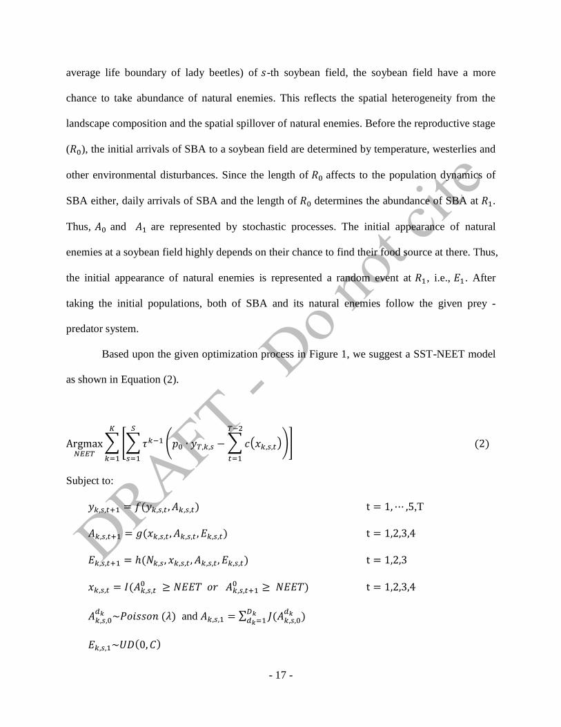
As an extension of Equation (1), Equation (2) is represented by a multi-year stochastic space-

time optimization model with heterogamous spatial domain. The state variables, potential yield

( ), SBA population density ( ), natural enemies density ( ) and , have the

subscript of a year ( ), a reproductive stage ( harvest) for a year and

a soybean field ( ). The objective function is now reflecting yearly discounting factor

( ). In natural enemies equation ( ( )), natural area proportion ( ) 4 is included to reflect

spatial spillover caused by the landscape composition. The initial distribution of natural enemies’

population density ( ) is assumed to follow the Discrete Uniform distribution whereas the

initial distribution of SBA population density ( ) is supposed to follow the Poisson

distribution. The distribution is determined by considering characteristic of random events5.

Before getting into prey - predator system, initial arrivals of SBA has an additional complex

stochastic process for period. If the first arrival of SBA happens at day 1 for -th year (

), then it starts breeding the next generation through reproduction function ( ). The same

processes are repeating a day before stage ( ). Thus, the initial distribution of SBA density at

is determined by the summation of all daily arrivals and their reproduced populations for

period. For the reproductive stages from to , both natural enemies’ and SBAs’

population density are described by the given prey - predator system not by a daily based process.

Equation (2) has two different variable definitions from Equation (1). The first is that

spraying decision is not a control variable but it is defined as a state variable through a

behavioral equation ( ), which is an indicator function. The addition of this behavioral equation

4 Natural area proportion ( ) does not vary within a growing season. Thus, it does not contain a reproductive

stage subscript ( ). 5 As discussed at the previous section, the initial appearance of natural enemies depends on their food sources and

thus, it is given as a pure random process for each soybean field. In the case of SBA, their initial arrivals are majorly

determined by westerlies and temperature. This is an exemplary case of Poisson point process.

- 19 -

is given by reflecting the reality of the limited information of SBA population density. Under

Zhang and Swinton’s (2009) assumption of Equation (1), the producer can observe complete

dynamics of population density of SBA with/without spraying for a whole growing season and

can choose the optimal spraying timing. Thus, the producer only cares spraying decisions which

support the maximum profit. In reality, however, producers can spray out chemical insecticides

when the scouting density or the expected density without spraying is more than NEET. The

suggested model in Equation (2) forces the producer spray when population density of SBA at

the beginning of a reproductive stage ( ) reaches to the NEET or when population density of

SBA without spraying at the end of a reproductive stage ( ) passes to the NEET. Thus,

Equation (2) gives a more realistic restriction of incomplete information of SBA density to a

producer than Equation (1) does.

The other difference in Equation (2) from Equation (1) is that the control variable of

Equation (2) is defined as NEET rather than spraying decision ( ). By changing the control

variable, we solve the NEET to maximize the profit that allows implementing comparison of

NEET from non-spatial and spatially explicit models by conditioning on Equation (2). Table 3

summarizes conditions and the derived models from Equation (2).

- Table 3 about here –

Spatial heterogeneity in pest control models can be spatially varying population densities of pests

or natural enemies, land composition, control costs and etc. In this study, the spatially varying

initial population density of SBA and its natural enemies are adopted to allow the comparisons of

the parallel studies. Since land composition is reflected into natural area proportion ( ),

- 20 -

geographical heterogeneity is considered as the same way in Bianchi and van der Werf (2003)

and Zhang et al. (2010). If we assume there is no spatially varying initial population density of

SBA and its natural enemies ( and ), Equation (2) is reduced to a homogenous spatial

model. Non-spatial models do not allow any spatial spillovers or spatial heterogeneity over

optimization process. Under the same homogeneous conditions from the homogeneous space

model, we can give a restriction as the spatial spillover parameter, which is a parameter of

natural area proportion ( ) in Equation (3), is equal to zero ( ) to derive non-spatial

model. Since the comparable study to the spatially explicit models (heterogeneous and

homogenous space models) maximize the profit/ha (Zhang and Swinton, 2009 and 2012), we set

up the objective function as per ha profit rather than total profit. For the comparison studies in

the next section, we calculate the average of total profit over total harvested areas from the two

spatially explicit models. By applying the same stochastic processes of the initial distribution of

SBA and its natural enemies, Equation (2) provides a way to compare the NEETs from non-

spatial and spatially explicit models.

IV. Numerical Experiments

It is rarely feasible to collect reliable size of sample to cover whole population of

optimization process of pest management or other types of biological invasion. Especially, SST-

NEET model proposed in this study requires a very long term samples which cover all study

regions to perform data based approaches by considering many different random events. To

overcome this difficulty, one of generally accepted solution is a simulation based approach. By

- 21 -

generating a representative virtual environment through computer, we can repeat the numerical

experiments with thousands of different simulations to support general conclusions. Based upon

the similar scenarios adopted in the previous studies, we perform numerical experiments of

optimization process for the suggested SST-NEET model.

4.1. Synthetic Geography

Regular grid cells are very general setup in biological invasion literature (Bianchi and

van der Werf (2003); Ding et al., 2007; Epanchin-Niell and Wilen (2012); Zhang et al., 2010). In

SBA studies, Bianchi and van der Werf (2003) create 16 ha (400m × 400m) with total 1,600 grid

cells of 10m × 10m cell). Among those, they assign 1%, 4% and 16% of total cells as squares-

shaped non-crop habitat with different fragmentation level of landscape composition. The other

cells are defined as homogenous soybean fields. Based upon the same geography in Bianchi and

van der Werf (2003), Zhang et al. (2010) extend the size to 1600 ha (4,000m × 4,000m) with

total 640,000 grid cells of 5m × 5m cells). By applying 10% natural area proportion, they use

6,400 cells as non-crop habitats with squares, strips and archipelago type landscape compositions.

The different shapes are given to each simulation separately. Even though studies are valuable to

test natural enemies’ role to suppress SBA over heterogeneous landscape composition, their

landscape composition may be too oversimplified to represent a real landscape. i.e., a combined

composition of all squares, strips and archipelago type are more realistic. The shape and

combinations of non-crop habitats can affect to spatial spillover of natural enemies population as

well. Considering the above disregarding factor, we generate a synthetic geography by using the

base concept in Zhang et al. (2010) as shown in Figure 2.

- 22 -

- Figure 2 about here –

We generate 1,600 ha area (4,000m × 4,000m) and each cell is given as 1 ha (10m × 10m) for

calculation simplicity. Similar to Zhang et al. (2010), about 10% (159 cells) are given as natural

areas but different shape of non-crop habitats are assigned over one landscape: one forest

(squares type: 81 cells), one river (strips type: 56 cells) and four hedgerows (archipelago type:

36 cells with four 9cells). And the other 1,441 (90%) cells are given as soybean monoculture

fields. Since each non-crop habitat can be a part of a large natural or semi-natural areas

connected to the outside of coordinates in Figure 2, we assign the natural area proportion ( )

of each soybean field by using a distance decay function. From the 2011 crop data layer (CDL)

of Newton County6 in IN, the soybean fields directly connected to natural areas are given as 48%

(the 90% of quartile of natural area proportion from the CDL), and the other soybean fields are

assigned a distance decayed values up to 0% over ten different distance intervals between 0 and

1,000m.

4.2. Numerical Model Specification

To demonstrate a feasibility of the suggested model of Equation (2), we specify a

numerical model of SBA example over the synthetic geography in Figure 2. This example is a

stochastic space-time extension of Zhang and Swinton (2009, 2012) and the results are

comparable to the parallel studies stated in Table 3. A social planer’s profit maximization from

soybean production can be given as:

6 For parameter estimation in the section 4.2., the field data collected from Newton County, IN is used. Data details

are in the next section.

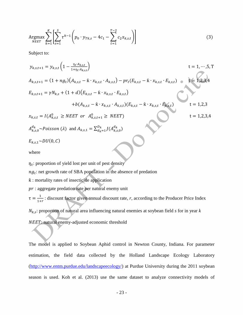
- 23 -

∑[∑ ( ∑

)

]

( )

Subject to:

(

)

( )( ) ( )

( )( )

( )( )

(

)

( ) and ∑ (

)

( )

where

: proportion of yield lost per unit of pest density

: net growth rate of SBA population in the absence of predation

: mortality rates of insecticide application

: aggregate predation rate per natural enemy unit

: discount factor given annual discount rate, r, according to the Producer Price Index

: proportion of natural area influencing natural enemies at soybean field s for in year k

: natural enemy-adjusted economic threshold

The model is applied to Soybean Aphid control in Newton County, Indiana. For parameter

estimation, the field data collected by the Holland Landscape Ecology Laboratory

(http://www.entm.purdue.edu/landscapeecology/) at Purdue University during the 2011 soybean

season is used. Koh et al. (2013) use the same dataset to analyze connectivity models of

- 24 -

conservation biological control agents. The summary of parameters is shown in Table 4 and

details explanations follows.

- Table 4 about here –

4.2.1. Prices and Costs

To get price and cost parameters in the optimization problem (3), we need to specify the

initial year. This is because all of the price parameters will be discounted to the initial time

period at the rate . Considering the fact that the field data was collected in 2011, prices for the

year 2011 are assumed to apply to the entire time horizon. The discount rate used is from the

Producer Price Index (PPI) from the Bureau of Labor Statistics7. From Table 2, it is clear that the

soybean reproductive stage ends around the beginning of September for each year. Thus, the 12

months unadjusted September PPI based on the September 2010-2011 period of 6.9% is used for

the parameter. Thus, the discrete discounting factor is given as =1/(1+0.069). The USDA

National Agricultural Statistic Services (NASS) reported soybean price ( ) in Newton County,

Indiana in 2011 was $0.4643/kg (=$12.50/bu).

As Song et al. (2006) mentioned, the spraying costs sensitively varies over region and

season. To derive constant spraying cost in the study area, we have reviewed several available

price source and chosen the average level of cost combination. The cost of spraying to control

SBA is consisted of two parts: a scouting cost ( ) and a spraying cost ( ). We assume that the

scouting happens at the beginning of each reproductive stages. Thus, there are total four times

7 Producer Price Index (PPI) is released as monthly base by the Bureau of Labor Statistics. http://www.bls.gov/ppi/

- 25 -

scouting and this is a fixed cost. On the other hand, spraying cost is a variable costs depending

on how many times spraying is implemented. Spraying cost consists of pesticides costs and

treatment costs. From the various sources, the total spraying costs are calculated as Table 5.

- Table 5 about here –

The spraying cost in Table 5, $21.89/ha(=$8.87/ac), is similar to the mid-range control cost of

$22.94 (=$9.29/ac) by Ragsdale et al. (2007) while it is lower than $24.69/ha (=$10/ac) by

Zhang and Swinton (2009).

4.2.2. Potential Yield

We follow the same function of potential yield equation ( ) and adopt the estimates of

the proportion of yield lost per unit of pest density ( ) in Zhang and Swinton (2009). They use

the rectangular hyperbolic model and get the estimates by the nonlinear least squares. Among

their estimates, has the negative value (-0.001) and they replace it as zero from the

assumption of non-compensation rule. This setup, however, may be unrealistic because it means

zero pest injury for R2 stage. To give a more realistic assumption, we use the value of

for . Since the R1 stage has only four-day median length in Table 2, we assume that

of the pest injury level continues to the R2 stage.

4.2.3. Population Dynamics of SBA

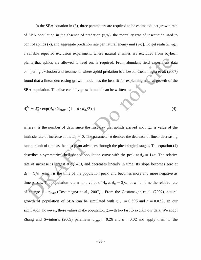
- 26 -

In the SBA equation in (3), three parameters are required to be estimated: net growth rate

of SBA population in the absence of predation ( ), the mortality rate of insecticide used to

control aphids ( ), and aggregate predation rate per natural enemy unit ( ). To get realistic ,

a reliable repeated exclusion experiment, where natural enemies are excluded from soybean

plants that aphids are allowed to feed on, is required. From abundant field experiment data

comparing exclusion and treatments where aphid predation is allowed, Costamagna et al. (2007)

found that a linear decreasing growth model has the best fit for explaining natural growth of the

SBA population. The discrete daily growth model can be written as:

( ( ( ))) (4)

where is the number of days since the first day that aphids arrived and is value of the

intrinsic rate of increase at the . The parameter denotes the decrease of linear decreasing

rate per unit of time as the host plant advances through the phenological stages. The equation (4)

describes a symmetrical bell-shaped population curve with the peak at . The relative

rate of increase is largest at , and decreases linearly in time. Its slope becomes zero at

, which is the time of the population peak, and becomes more and more negative as

time passes. The population returns to a value of at , at which time the relative rate

of change is (Costamagna et al., 2007). From the Costamagna et al. (2007), natural

growth of population of SBA can be simulated with and . In our

simulation, however, these values make population growth too fast to explain our data. We adopt

Zhang and Swinton’s (2009) parameter, and and apply them to the

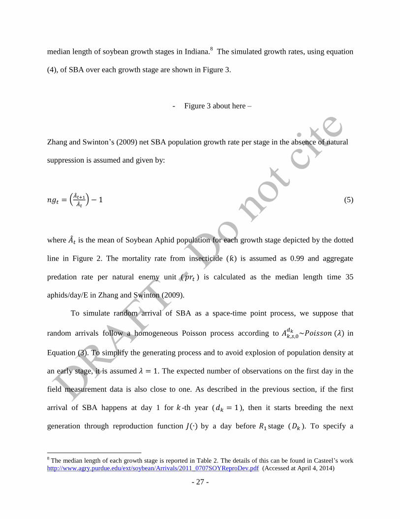
- 27 -

median length of soybean growth stages in Indiana.8 The simulated growth rates, using equation

(4), of SBA over each growth stage are shown in Figure 3.

- Figure 3 about here –

Zhang and Swinton’s (2009) net SBA population growth rate per stage in the absence of natural

suppression is assumed and given by:

(

) (5)

where is the mean of Soybean Aphid population for each growth stage depicted by the dotted

line in Figure 2. The mortality rate from insecticide ( ) is assumed as 0.99 and aggregate

predation rate per natural enemy unit ( ) is calculated as the median length time 35

aphids/day/E in Zhang and Swinton (2009).

To simulate random arrival of SBA as a space-time point process, we suppose that

random arrivals follow a homogeneous Poisson process according to ( ) in

Equation (3). To simplify the generating process and to avoid explosion of population density at

an early stage, it is assumed . The expected number of observations on the first day in the

field measurement data is also close to one. As described in the previous section, if the first

arrival of SBA happens at day 1 for -th year ( ), then it starts breeding the next

generation through reproduction function ( ) by a day before stage ( ). To specify a

8 The median length of each growth stage is reported in Table 2. The details of this can be found in Casteel’s work

http://www.agry.purdue.edu/ext/soybean/Arrivals/2011_0707SOYReproDev.pdf (Accessed at April 4, 2014)

- 28 -

function , we use Equation (4) but the equation is now defined as daily SBA population density

with predation and spraying. Since the field measurement data was collected with predation by

natural enemies and spraying, we can estimate equation (4) as a population dynamics equation of

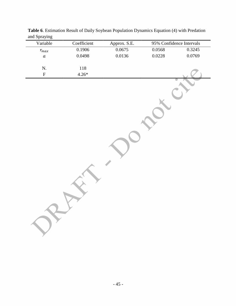
SBA with predation and spraying. Because of inclusion of predation and spraying, we can reduce

dynamics of natural enemies and spraying in this stage. Nonlinear least squares estimation of

equation (4) yields the results in Table 6.

- Table 6 about here –

For simulation of the initial distribution of SBA, random Poisson process in Equation (3) is

implemented first for all soybean fields at each year. The estimated parameters from Table 6 are

used in growth equation (4) to simulate each day and the cumulative summation over time before

stage is calculated.

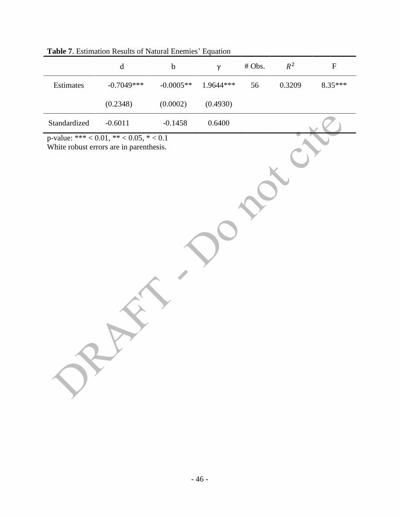
4.2.4. Population Dynamics of Natural Enemies

Population dynamics of natural ermines in Equation (3) are modeled using the well-

known Lotka-Volterra prey-predator equation that was adopted previously by Zhang and

Swinton (2009). To estimate the net decline rate ( ), the reproduction rate ( ) and spatial

spillover parameter ( ) on abundance of natural enemies, we set up a descriptive relationship of

Equation (6) similar to Zhang and Swinton (2009).

(6)

- 29 -

where . Because of data limitation, we use only and stage field

measurement data and give an assumption that the estimates of (6) is universal for all

reproductive stages. By using White error correction, the Least Squares estimation results are

shown in Table 7.

- Table 7 about here –

To simulate the initial appearance of natural enemies ( ), the discrete uniform

distribution is assumed. We setup for the simulations of the initial appearance of natural

enemies.

4.3. Solution Method

Dynamic optimization generally can be solved by Hamilton-Jacobi-Bellman (HJB)

equation. The dynamic problem in (3), however, includes discrete variables: the positive integer

of NEET and the binary decision to spray. Thus, gradient-based approaches are not suitable for

this type of problem. The discrete representation of spatial domain adds an additional

computation issues as well. The optimal control models combined with discrete domains and

variables are called integer programming and the solution paths can be found through dynamic

programming or discrete numerical boundary value solution techniques. Among those, Zhang

and Swinton (2009, 2012) used a numerical calculation based on a set of optimal control paths

which finds the solutions after calculating all of the possible combinations of control variables.

- 30 -

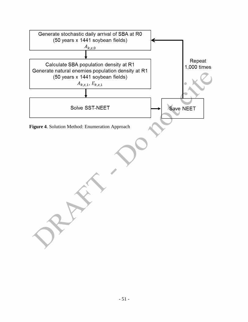
We adopt this enumeration approach to solve our optimization problem in (4). Figure 4 shows

the process used to find solutions.

- Figure 4 about here –

We are solving infinite time horizon optimal control solution in Equation (4). By applying for the

methods in Epanchin-Niell and Wilen (2012), we redefine the infinite time horizon as the finite

time domain. We choose large enough so that the decision rules and equilibrium values

are not sensitive to changes of . Thus, Equation (4) become a finite year optimal control model.

In the simulation, at first, we generate stochastic daily arrival of SBA at stages which

contains 50 years times 1,441 soybean fields’ random number generation. Using the initial

distribution equation of SBA, we calculate SBA population density at . From the discrete

uniform distribution, we generate the initial distribution of natural enemies’ density at , which

includes 50 years times 1,441 soybean fields’ random number generation as well. After these two

stochastic processes, we solve SST-NEET in Equation (4) by increasing the NEET from 1 to 500

and save the optimal NEET number. To support many different initial distribution scenarios, we

repeat the same process 1,000 times. By giving the restrictions in Table 3, we find 1,000 scenario

NEET solutions for homogeneous space and non-spatial models either to perform comparison

analysis.

For the SST-NEET model, there are in total 36,025,000,000 calculations (=1,000

scenarios × 50 years × 1,441 soybean fields × 500 NEET). Through HASEN-A cluster of Rosen

Center for Advanced Computing at Purdue, 96 cores (2.3 GHz) take approximately 33 hours and

21 minutes. In a general integer programming, researchers often encounter intractable dimension

- 31 -

problem so called the curse of dimensionality. If this problem comes out, then the enumeration

approach is not applicable anymore. For this case, the solver, Solving Constraint Integer

Programs (SCIP) provides a feasible way (Achterberg, 2009).

V. Results

We implement non-spatial, homogeneous space and heterogeneous space optimal control

model of Equation (3) with the same 1,000 initial arrival scenarios of SBA and natural enemies.

The derive SST-NEET results are shown in Figure 5.

- Figure 5 about here –

Two spatially explicit models (Heterogeneous space and Homogeneous space) are maximizing

the total profit while non-spatial model are maximizing total profit / ha. To make them

comparable, we calculate the average total profit over total harvest areas for 50 years in the

spatially explicit model. In Figure 5, the maximum values of profits for each initial distribution

scenario are drawn as a line by increasing SST-NEET from 0 to 500. The median values of profit

following by increased NEET are the blue line and 95% confidence intervals of the median are

the two black lines. The optimum SST-NEET is represented by the red vertical line. Form the

simulations, the optimum of spatially heterogeneous SST-NEET shows the highest value (40

aphids/plant). The optima from spatially explicit models are higher than the optimum of non-

spatial SST-NEET.

- 32 -

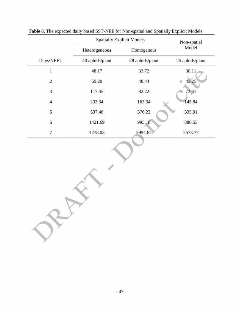
The SST-NEET in this study and NEET in Zhang and Swinton (2009, 2012) are based on

the reproductive stage whereas the ET in Ragsdale at al. (2007) is based on the daily growth

stage. Thus, these are not directly comparable to each other. From Table 2, we use the median

length of each reproductive stage in Equation (3). Thus, if we apply the results of Table 6 into

Equation (4) backwardly, we can derive the daily based SST-NEET that is possibly comparable

to the ET. Since spraying decisions are available on to and the behavioral equation of

spraying in Equation (3) is decided by

, the maximum lead

times are five days. For example of stage with 10 days the median length, the agent waits to

spray until will exceed the NEET value if is less than the NEET. Besides, the agent

will spray if she expects that of one of any day in will pass the NEET without spraying.

Thus, the maximum lead times are the median length of the longest mid-time among to ,

i.e., five days. Table 8 shows the daily based expected SST-NEET for each models.

- Table 8 about here –

The five-day lead times SST-NEET in Table 8 from non-spatial model can be compared to

Ragsdale et al. (2008). We apply the higher soybean price, $0.4643/kg (=$12.50/bu) than

$5.50/bu, $6.00/bu, or $6.50/bu in Ragsdale et al. (2008) while the the cost of control ($21.89/ha)

in this study is lower than the middle level of costs of control ($24.51/ha) in Ragsdale et al.

(2008). In the concept of EIL and ET, the higher soybean price leads the lower ET while the

lower cost of control derives the higher ET. Considering this trend, the calculated daily expected

SST-NEET for non-spatial model in Table 8 can be seen as a congruent value from the Ragsdale

- 33 -

et al. (2008). From the almost doubled soybean price, 336 aphids/plant is higher than 273±38

aphids/plant but it is still less than two times standard deviation ranges in Ragsdale et al. (2008).

From Table 8, we can see that spatially explicit models deter spraying decision because

of the higher SST-NEET of two models than the SST-NEET of non-spatial model. Even more

interestingly, the heterogeneous SST-NEET has 537 aphids/plant that is much higher than 376

aphids/plant in the homogeneous SST-NEET. Up to five days lead time, the homogeneous SST-

NEET shows the similar level to the non-spatial SST-NEET. If we consider the expected initial

distributions of SBA and natural enemies are the same in heterogeneous and homogeneous

models in enough size of different scenarios, this means that increasing heterogeneity over space

bring the more effective suppression of pests by ecosystem services. Since the initial

distributions of SBA and natural enemies are determined by the environmental disturbance, a

feasible way of taking the more advantage of ecosystem services is increasing spatial spillover

effects. In terms of policy means, this conclusion supports the fact that CP policies can be an

effective way by using the ecosystem services on pest control.

VI. Conclusion and Future Steps

This study develops and solves a stochastic, multi-year, discrete space-time optimal

control model that allows the comparative analysis between non-spatial and spatially explicit

models. The suggested model, named Stochastic Space-Time Natural Enemy-adjusted Economic

Threshold (SST-NEET), is designed to include a prey-predator system between a biological

invader pest and its natural enemies, and an economic agent’s behavioral optimization of

- 34 -

spraying decision. By suggesting a unified framework for handling simultaneous complexities in

optimal control models of biological invasion, this study finds the following three conclusions

through numerical simulation experiments with the field collected data.

First, the optimal control model of biological invasion needs to be considered

simultaneous complexities in the unified framework. There have been much of the previous

studies including some parts of stochastic, space and time dynamics. Even though their

approaches are successful to show one or more of components are important in the biological

invasion process, the crucial aspect of biological invasion is that multi-year stochastic space time

dynamics happens simultaneously. To avoid oversimplifying bias, this study suggests the model

that is possible to include major four complexity components in a unified model.

Second, the suggested SST-NEET is the most generalized version of the spatially explicit

NEET model. The SST-NEET can be simply reduced to spatially homogenous or non-spatial

model by giving conditions of each model assumed. Through the numerical simulation

experiments, we show that this unified framework is working well to implement comparison

analysis.

Finally, accounting for spatial heterogeneity and spatial spillovers are important factors to

consider when making pest control decisions. The numerical experiments show that the spatially

heterogeneity deters the SST-NEET notably from the spatially homogenous or non-spatial SST-

NEET. Considering the fact that the initial distribution of pests and natural enemies are

determined by the environmental disturbance, the increasing spatial spillovers can be an effective

way to use ecosystem services to manage biological invasion. This means that installation CP

makes agroecosystem services more effective and net benefit from CP installation can be higher

- 35 -

than spray. Thus, installation of CPs can be an economically better way to control Soybean

Aphid instead of spraying.

Since this study is still ongoing process, a general process to rigorously test validity of

the suggested model is still underway. The following future steps for analysis are planned:

including CP installation scenarios on the SST-NEET simulation; and implementing an extensive

sensitivity analysis of simulation parameters; and performing economically meaningful scenario

analysis.

Acknowledgements

This publication was made possible by USDA-NIFA, AFRI 2009 (EPA-G2008-STAR-K1)

Enhancing Ecosystem Services from Agricultural Lands: Management, Quantification, and

Developing Decision Support Tools. Its contents are solely the responsibility of the grantee and

do not necessarily represent the official views of the USEPA or USDA. Further, neither USEPA

nor USDA endorses the purchase of any commercial products or services mentioned in the

publication.

- 36 -

References

Achterberg, T. (2009). SCIP: Solving Constraint Integer Programs. Mathematical Programming

Computation. 1. 1-41.

Ando, W. A. and K. Baylis. (2012). Spatial Environmental and Natural Resource Economics. In

Fischer, M. M. and Nijkamp P. (eds.). 1029-1048. Handbook of Regional Science.

Springer. Germany: Hiedelberg.

Bianchi, F. J. J. A., C. J. H. Booij, and T. Tscharntke. (2006). Sustainable Pest Regulation in

Agricultural Landscapes: A Review on Landscape Composition, Biodiversity and Natural

Pest Control. Proceedings of the Royal Society of London Series B – Biological Sciences.

273. 1715-1726.

Bianchi, F. J. J. A. and W. van der Werf . (2003). The Effect of the Area and Configuration of

Hibernation Sites on the Control of Aphids by Coccinella septempunctata (Coleoptera:

Coccinellidae) in Agricultural Landscapes: A Simulation Study. Environmental

Entomology. 32(6). 1290-1304.

Billionnet, A. (2013). Mathematical Optimization Ideas for Biodiversity Conservation. European

Journal of Operational Research. 231. 514-534.

Bockstael, N. E. (1996). Modeling Economics and Ecology: The Importance of a Spatial

Perspective. American Journal of Agricultural Economics. 78. 1168-1180.

Brock, W. and A. Xepapadeas. (2004). Spatial Analysis: Development of Descriptive and

Normative Methods with Applications to Economic –Ecological Modelling. University of

Wisconsin, Department of Economics SSRI Working Paper #2004-17.

Brock, W. and A. Xepapadeas. (2008). Diffusion-induced Instability and Pattern Formulation in

Infinite Horizon Recursive Optimal Control. Journal of Economic Dynamics and Control.

32(9). 2745-2787.

Brock, W. and A. Xepapadeas. (2010). Pattern Formation, Spatial Externalities and Regulation in

Coupled Economic-Ecological Systems. Journal of Environmental Economics and

Management. 59. 149-164.

Costamagna, A. C. and W. van der Werf, F. J. J. A. Bianchi, and D. A. Landis. (2007). An

exponential growth model with decreasing r captures bottom-up effects on the population

growth of Aphis glycines Matsumura (Hemiptera: Apphididae). Agricultural and Forest

Entomology. 9. 297-305.

- 37 -

Cressie, N. and C. K. Wikle. (2011). Statistics for Spatio-Temporal Data. Wiley.

Ding, W., L. J. Gross, K. Langston, S. Lenhart, and L. A. Real. (2007). Rabies in Raccoons:

Optimal Control for a Discrete Time Model on a Spatial Grid. Journal of Biological

Dynamics. 1(4). 379-393.

Epanchin-Niell, R. S. and J. E. Wilen. (2012). Optimal Spatial Control of Biological Invasion.

Journal of Environmental Economics and Management. 63. 260-270.

Fenichel, E. P., R. D. Horan, and J. R. Bence. (2010). Indirect Management of Invasive Species

through Bio-controls: A Bioeconomic Model of Salmon and Alewife in Lake Michigan.

Resource and Energy Economics. 32. 500-518.

Gardiner, M. M., D. A. Landis, C. Gratton, N. Schmidt, M. O’Neal, E. Muller, J. Chacon, G. E.

Heimpel, and C. D. DiFonzo. (2009). Landscape composition influences patterns of

native and exotic lady beetle abundance. Diversity and Distributions. 15. 554-564.

Goh, B. S., G. Leitmann, and T. L. Vincent. (1974). Optimal Control of a Prey-Predator System.

Mathematical Bioscience. 19. 263-286.

Helpern, B. S., H. M. Regan, H. P. Possingham, and M. A. McCarthy. (2006). Accounting for

Uncertainty in Marine Reserve Design. Ecology Letters. 9(1). 2-11.

Horan, R. D., E. P. Fenichel, K. L. S. Drury, and D. M. Lodge. (2011). Managing Ecological

Thresholds in Coupled Environmental-Human Systems. Proceedings of the National

Academy of Sciences of the United States of America (PNAS). 108(18). 7333-7338.

Koh, I. S., H. I. Rowe, and J. D. Holland. (2013). Graph and circuit theory connectivity models

of conservation biological control agents. Ecological Applications. 23(7). 1154-1573.

Landis, D. A., S. D. Wratten, and G. M. Gurr. (2000). Habitat Management to Conserve Natural

Enemies of Arthropod Pests in Agriculture. Annual Review of Entomology. 45. 175-201.

Liu, S., D. Cook, A. Diggle, A. B. Siddique, H. Hurley, and K. Lowell. (2009). Using Dynamic

Ecological-economic Modeling to Facilitate Deliberative Multicriteria Evaluation

(DMCE) in Quantifying and Communicating Bio-invasion Uncertainty. 18th

World

IMACS / MODSIM Concgress, Cairns, Australia 13-17. July 2009.

Mahul, O. and A. Gohin. (1999). Irreversible Decision Making in Contagious Animal Disease

Control under Uncertainty: An Illustration using FMD in Brittany. European Review of

Agricultural Economics. 26(1). 39-58.

- 38 -

Meehan, T. D., B. P. Werling, D. A. Landis, and C. Gratton. (2012). Pest-suppression potential

of Midwestern landscapes under contrasting bioenergy scenarios. PLos ONE. 7(7).

E41728. 1-7.

Millennium Ecosystem Assessment Board. (2005). Ecosystem and Human Well-being. The

Mullennum Ecosystem Assesment Series. Island Press.

URL: http://www.esajournals.org/doi/abs/10.1890/12-1595.1 (Accessed at 4. 30.2014.)

Olson, L. J. and S. Roy. (2002). The Economics of Controlling a Stochastic Biological Invasion.

American Journal of Agricultural Economics. 84(5). 1311-1316.

Perrings, C., M. Williamson, and S. Dalmazzone. (2000). The Economics of Biological Invasion.

Edward Elgar Publisher. UK: Cheltenham.

Pimentel, D. (2002). Biological Invasions: Economic and Environmental Costs of Alien Plant,

Animal, and Microbe Species. CRC press. US: Boca Raton.

Ragsdale, D. W., B. P. McCornack, R. C. Venette, B. D. Potter, I. V. MacRae, E. W. Hodgson,

M. E. O. O’Neal, K. D. Johnson, R. J. O’Neal, C. D. DiFonzo, T. E. Hunt, P. A. Glogoza,

and E. M. Cullen. (2007). Economic Threshold for Soybean Aphid (Hemiptera:

Aphididae). Journal of Economic Entomology. 100(4). 1258-1267.

Refsgaard, J. C., J. P. van der Sluijs, A. L. Højberg, and P. A. Vanrolleghem. (2007). Uncertainty

in the Environmental Modelling Process – A Framework and Guidance. Environmental

Modelling & Software. 22. 1543-1556.

Sanchirico, J. N. and J. E. Wilen. (1999). Bioeconomics of Spatial Exploitation in a Patchy

Environment. Journal of Environmental Economics and Management. 37. 139-150.

Smith, G. S. and D. Pike. (2002). Soybean pest management strategic plan. U.S. Department of

Agriculture North Central Region Pest Management Center and United Soybean Board.

http://www.ipmcenters.org/pmsp/pdf/RCSoybeanPMSP.pdf (Accessed at 4. 30.2014.)

Smith, M. D., J. N. Sanchirico, and J. E. Wilen. (2009). The Economics of Spatial-dynamic

Process: Application to Renewable Resources. Journal of Environmental Economics and

Management. 57. 104-121.

Song, F., S. M. Swinton, C. D. DiFonzo, M. O’Neal, and D. W. Ragsdale. (2006). Profitability

Analysis of Soybean Aphid Control Treatments in Three North-Central States.

Department of Agricultural Economics Staff Paper. No. 2006-24. Michigan State

University. http://ageconsearch.umn.edu/handle/11489 (Accessed at 4. 30.2014.)

- 39 -

Stern, V. M., R. F. Smith, K. van den Bosch, K. S. Ragen. (1959). The integrated control concept.

Hilgardia. 29. 81-101.

Venette, R. C. and D. W. Ragsdale. (2003). Assessing the invasion by Soybean Aphid

(Homopters: Aphididae): where will it end? Annals of the Entomological Society of

America. 97(2). 219-226.

Zhang, W. and S. M. Swinton. (2009). Incorporating natural enemies in an economic threshold

for dynamically optimal pest management. Ecological Modeling. 220(9). 1315-1324.

Zhang, W. and S. M. Swinton. (2012). Optimal control of soybean aphid in the presence of

natural enemies and the implied value of their ecosystem services. Journal of

Environmental Management. 96(1). 7-16.

Zhang, W., W. van der Werf, and S. M. Swinton. (2010). Spatially Optimal Habitat Management

for Enhancing Natural Control of an Invasive Agricultural Pest: Soybean Aphid.

Resource and Energy Economics. 32(4). 551-565.

- 40 -

Table 1. Comparison of Economic Thresholds

Study Typea

ET/NEET (aphids/plant)

Time Spaceb Stochasticity

Ragsdale et al. (2007) ET 273 ± 38 Single Season Non-Spatial No

McCarville et al. (2011) ET 250 Single Season Non-Spatial No

Zhang and Swinton (2009) NEET 140 Single Season Non-Spatial No

Zhang and Swinton (2012) NEET varies Single Season Non-Spatial No

Zhang et al. (2010) NEET Not stated Single Season Homogeneous No

a If the study includes natural enemies’ equation explicitly, then it is classified to NEET.

b Non-Spatial models do not include spatial analysis. The homogeneous space means that all

crop fields have the same initial distribution of SBA population density, and the non-crop

habitats are given as the fixed initial distribution of natural enemies’ population density.

- 41 -

Table 2. Observed Duration of Soybean Reproductive Stage in Indiana for 10 years, 2002 - 2011

Stagea R1 R2 R3 R4 R5 R6 First

Observed Soybean

Aphidb

Aphid (O)

/ Non-Aphid (X)

Yearb

Planted

Area

(1,000ac)a

Soybean

Production

(1,000 bu)a Median

Duration

4 10 10 10 15 20

begins ends begins ends begins ends begins ends begins ends begins ends

2011 6/27/2011 6/30/2011 7/1/2011 7/10/2011 7/11/2011 7/20/2011 7/21/2011 7/30/2011 7/31/2011 8/14/2011 8/15/2011 9/3/2011 7/29/2011 X 61.6 3004

2010 6/21/2010 6/24/2010 6/25/2010 7/4/2010 7/5/2010 7/14/2010 7/15/2010 7/24/2010 7/25/2010 8/8/2010 8/9/2010 8/28/2010 7/23/2010 X 64.5 3254

2009 6/30/2009 7/3/2009 7/4/2009 7/13/2009 7/14/2009 7/23/2009 7/24/2009 8/2/2009 8/3/2009 8/17/2009 8/18/2009 9/6/2009 6/12/2009 X 67.3 3266.6

2008 6/22/2008 6/25/2008 6/26/2008 7/5/2008 7/6/2008 7/15/2008 7/16/2008 7/25/2008 7/26/2008 8/9/2008 8/10/2008 8/29/2008 6/13/2008 X 66.4 3397.3

2007 6/25/2007 6/28/2007 6/29/2007 7/8/2007 7/9/2007 7/18/2007 7/19/2007 7/28/2007 7/29/2007 8/12/2007 8/13/2007 9/1/2007 5/23/2007 O 56.8 2857.5

2006 7/3/2006 7/6/2006 7/7/2006 7/16/2006 7/17/2006 7/26/2006 7/27/2006 8/5/2006 8/6/2006 8/20/2006 8/21/2006 9/9/2006 6/6/2006 X 76.2 3748.2

2005 6/20/2005 6/23/2005 6/24/2005 7/3/2005 7/4/2005 7/13/2005 7/14/2005 7/23/2005 7/24/2005 8/7/2005 8/8/2005 8/27/2005 5/26/2005 O 72.5 3564.7

2004 6/21/2004 6/24/2004 6/25/2004 7/4/2004 7/5/2004 7/14/2004 7/15/2004 7/24/2004 7/25/2004 8/8/2004 8/9/2004 8/28/2004 6/11/2004 X 73.4 3783.4

2003 7/1/2003 7/4/2003 7/5/2003 7/14/2003 7/15/2003 7/24/2003 7/25/2003 8/3/2003 8/4/2003 8/18/2003 8/19/2003 9/7/2003 6/11/2003 O 76.8 2447.4

2002 6/24/2002 6/27/2002 6/28/2002 7/7/2002 7/8/2002 7/17/2002 7/18/2002 7/27/2002 7/28/2002 8/11/2002 8/12/2002 8/31/2002 6/18/2002 X 77.8 3875.6

a USDA NASS, 2002-2011

b Purdue Entomology Extension weekly online newsletter, http://extension.entm.purdue.edu/pestcrop/

- 42 -

Table 3. Conditions and Various Models from the SST-NEET

Heterogeneous Space

Equation (2) Homogenous Space Non-Spatial Model

SBA

Natural Enemies

Natural Area Spatial Spillover

Parametera ( ) ≠ 0

Spatial Spillover

Parameter ( ) ≠ 0

Spatial Spillover

Parameter ( ) = 0

Maximization Total Profit Total Profit Profit/ha

Parallel ETb

Studies .

Bianchi and van der

Werf (2003) /

Zhang et al. (2010)

Ragsdale et al. (2007) /

Zhang and Swinton

(2009, 2012) a Spatial Spillover Parameter ( ) is in Equation (3).

b ET: Economic Threshold

- 43 -

Table 4. Summary of Parameters

Parameter Value Meaning Source

r 0.069 Producer Price Index (PPI) Bureau of Labor Statistics

$0.4643/kg Initial soybean price USDA NASS

$19.76/ha Scouting cost Table 5 in this study

$21.89/ha Spray cost Table 5 in this study

Proportion of yield lost per unit

of pest density for each stage Zhang and Swinton (2009)

Net growth rate of SBA

population in the absence of

predation

Calculated using

Costamagna et al. (2007) and

Zhang and Swinton (2009)

Aggregate predation rate per

natural enemy unit

Zhang and Swinton (2009):

35 SBAs/day/E

0.99 mortality rate of insecticide Zhang and Swinton (2009)

1.9644 Spatial spillover of E Table 6 in this study

-0.7049 Net decline rate of E Table 6 in this study

-0.0005 Reproduction rate of E Table 6 in this study

1 Intensity of SBA arrival Newton County data

1 Maximum appearance of E Honěk (1989)

- 44 -

Table 5. Total Treatment Costs of SBA Management

Inputs Source Price Application

Rate

Costs for

the acre

Pesticides

(Lambda-

Cyhalothrin)

Makhteshim Agan

of North Americaa

$38.80/gallon $8.00oz/ac $5.99/ha

Treatment Purdue Extensionb $15.90/ha

Spraying $21.89/ha

Scouting Song et al. (2006) $4.94/scout Four times $19.76/ha

a The price can be referred to http://www.cdms.net/LDat/ld0HL020.pdf

b Purdue Extension: Chemical Application 2013 Indiana Farm Custom Rates,

https://www.ces.purdue.edu/extmedia/EC/EC-130-W.pdf

- 45 -

Table 6. Estimation Result of Daily Soybean Population Dynamics Equation (4) with Predation

and Spraying

Variable Coefficient Approx. S.E. 95% Confidence Intervals

0.1906 0.0675 0.0568 0.3245

0.0498 0.0136 0.0228 0.0769

N. 118

F 4.26*

- 46 -

Table 7. Estimation Results of Natural Enemies’ Equation

# Obs. F

Estimates -0.7049*** -0.0005** 1.9644*** 56 0.3209 8.35***

(0.2348) (0.0002) (0.4930)

Standardized -0.6011 -0.1458 0.6400

p-value: *** < 0.01, ** < 0.05, * < 0.1

White robust errors are in parenthesis.

- 47 -

Table 8. The expected daily based SST-NEE for Non-spatial and Spatially Explicit Models

Spatially Explicit Models Non-spatial

Model

Heterogeneous Homogenous

Days/NEET 40 aphids/plant 28 aphids/plant 25 aphids/plant

1 48.17 33.72 30.11

2 69.20 48.44 43.25

3 117.45 82.22 73.41

4 233.34 163.34 145.84

5 537.46 376.22 335.91

6 1421.69 995.18 888.55

7 4278.03 2994.62 2673.77

- 48 -

Figure 1. Dynamics of the Suggested Stochastic Space-Time Optimization Model

Note: This figure is a conceptual extension of Fig. 1 in Zhang and Swinton (2009, p. 1317.).

- 49 -

Figure 2. Synthetic Geography

- 50 -

Figure 3. Natural Growth of Soybean Aphid Population with and

- 51 -

Figure 4. Solution Method: Enumeration Approach

- 52 -

Figure 5. Results of SST-NEET: Non-spatial, Homogeneous Space and Heterogeneous Space