dynamic model of a bicycle with a balancer and its control
TRANSCRIPT

Proceedings, Bicycle and Motorcycle Dynamics 2010Symposium on the Dynamics and Control of Single Track Vehicles,
20–22 October 2010, Delft, The Netherlands
Dynamic Model of a Bicycle with a Balancer and Its Control
L. Keo∗, M. Yamakita∗
∗ Department of Mechanical and Control EngineeringTokyo Institute of Technology
2-12-1 Ookayama, Meguro-Ku, Tokyo 152-8552, Japane-mail: {lychek,yamakita}@ac.ctrl.titech.ac.jp
ABSTRACT
In this paper we present the dynamic model of a bicycle with a balancer and itsbalancing control.A new configuration balancer that it can be use as a balancer or a flywheel by shifting the center ofgravity of the balancer is also presented. This balancer configuration is changed according to thesituation of the bicycle system, which corresponds to the change of the dimension of the system.Stabilizing bicycle with the flywheel has better performance than the balancerbut it cannot controlto shift the bicycle angle to track the desired value, unlike the balancer whichcan do this motion.The balancer is configured as a flywheel, when disturbances to the system are large, and it willswitch to the balancer when we want to shift the bicycle body angle. The simplified model of thebicycle with the balancer is derived from Lagrangian and nonholonomic constraints with respectto translation and rotation relative to the ground plane. The balancing control is derived based onthe output-zeroing controller. Numerical simulation and experimental results are shown to verifythe effectiveness of the proposed control strategy.
Keywords: Bicycle with Balancer Modeling; Balancing Control; Output-Zeroing; Balancer;Flywheel.
1 Introduction
Research on the stabilization of bicycles has been gained momentum over the last decade in a num-ber of robotic laboratories around the world. Modeling and control of bicycles became a populartopic for researchers in the latter half of the last century. The bicycle literatures are comprehen-sively reviewed from a control theory perspective in [1] and in [2], which also describe interestingbicycle-related experiments. A. L. Schwab et al. [3] developed the linearized equations of motionfor a bicycle as a benchmark and it is suitable for research or application.It is well known thatthe balancing control of bicycle with steering at zero or slow linear velocity isvery difficult [4].Thus, we are interested to stabilize the bicycle with the balancer that it can allowus to control thebicycle at zero or slow linear velocity.In this paper, we present the development of a bicycle with a balancer andthe balancing controlin our laboratory. The first generation of the bicycle with balancer (Fig.1) was developed by M.Yamakita in 2005 [5] by using Lagrange dynamic equations and the balancing control used anoutput function which is defined by an angular momentum and the new state function is controlledto zero. We reported the experimental study of automatic control of bicycle with a balancer in [6]and [7]. The cooperation control for stabilization of an autonomous bicycle with both steering andbalancer was presented in [8] and [9]. The results of balancing bicycle with a steering handlebarand a balancer, it was shown that it has better performance than balancing control of a bicycle withonly a balancer. In order to control the bicycle in narrow place, we introduced acrobatic turn via

Figure 1. Bicycle with a balancer system.
wheelie motion that it can allow the bicycle turn on the back wheel at zero linearvelocity as shownin Fig.2 and it is presented in [10]. This system is still in the development of experiment and wewill report the results in the future. In addition to extending those results to balancing the bicycle,
Figure 2. Perform a wheelie on a bicycle with a balancer.
we propose a new balancer configuration [11] for stabilizing of an unmanned bicycle that it showsin Fig.3. In Fig. 3 shows a bicycle experimental setup which has a new balancer configuration onit. This new balancer has two motors, one is a rotating motor which is used to rotatethe balancer.The another motor is a linear motor which is used to shift the center gravity of thebalancer. Withthese configurations, we can use the balancer as a flywheel mode (Fig.4a) or a balancer mode(Fig. 4b). The advantage of the flywheel is to stabilize the bicycle with large region of stability.The advantages of the balancer are to shift the bicycle body from obstacles and to control the bicy-
2

Figure 3. Bicycle with flywheel balancer hardware.
(a) Flywheel mode (b) Balancer mode
Figure 4. Flywheel balancer configurations.
cle to follow the trajectory with high speed. This paper is composed of six sections. In section II,we present a simplified dynamic model of the bicycle with the balancer. In section III, we discusscontrol system design for stabilizing the bicycle. Numerical simulation and experimental resultsare presented in section IV and V, respectively. The conclusions are summarized in section VI.
2 Bicycle with Balancer Dynamics
In this section, we will present a bicycle with a flywheel balancer model based on an invertedpendulum model. A detailed model of a bicycle is complex since the system has many degreesof freedom. The coordinate system used to analyze the bicycle is defined inFig. 5. We considerthe bicycle as a point mass with two wheel contacts with the ground, and we consider the bicycleand the balancer as a two link system where the first link is the bicycle body withsteering and thesecond link is the balancer. We will defineα as the roll angle andβ as the balancer angle. Thebicycle and the balancer parameters are shown in Table I. These parameters were identified froman experimental setup. The height of the balancer to the center of gravity (hb) varies from0m to
3

Table 1. The bicycle with balancer parametersParameter descriptions Par. Value
Bicycle mass m 45kgHeight of the bicycle center of mass h 0.5mMoment inertia of bicycle at COG I 0.81kgm2
Distance between ground and balancerl 0.87mBalancer mass mb 11.72kg
Moment inertia of balancer at COG Ib 0.49kgm2
0.14m and the balancer becomes flywheel whenhb is zero. From [13], we can obtain the bicycle
Flywheel Balancer
Linear Motor
z
α
CG
h
l
β
y
O
x
Figure 5. Coordinate system of the bicycle with the balancer.
with flywheel dynamics model as[
M11 M12
M21 M22
] [
α
β
]
=
[
K1
K2
]
+
[
01
]
τb, (1)
whereτb is the balancer torque input and
M11 = I + Ib +mh2 +mb(h2b + l2 + 2hbl cos(β)),
M12 = M21 = Ib + hbmb(hb + l cosβ),
M22 = Ib + h2bmb,
K1 = hmg sinα+mb(g(l sinα+ hb sin(α+ β))
+hblβ(2α+ β) sinβ),
K2 = hbmb(−lα2 sinβ + g sin(α+ β)).
This gives us a simplified model that we can use to design the controllers for the bicycle stabiliza-tion.
4

3 Balancing Control Algorithm
In this section, we design output-zeroing controller to stabilize the bicycle with flywheel or bal-ancer. The basic idea of output-zeroing controller is that an output function is defined so that therelative degree from input to the output becomes three and the zero dynamic becomes stable. Then,the output-zeroing controller is designed. In this case, a new state is defined then the new outputfunction is easily determined since the angular momentum is integrable for two D.O.F. system.
3.1 Model of two-link system
By projecting the motion of the balancer onY Z plane, the system can be considered as a two-linksystem (Fig.6). In the two-link model, the bicycle body and steering handlebar consist ofthe first
Linear Motor
mb
h
α
hb
m
Passive joint
z
y
β
l
Active joint
Balancer
CG
Figure 6. Two-Link System.
link and the balancer with the linear motor is considered as the second link. Thecontrol torque forthe system is only applied to the second joint of the balancer. We can find the angular momentumL from the first row of equation (1) as
L = M11α+M12β (2)
= (d1 + d3 + 2d2 cosβ) α+ (d3 + d2 cosβ) β,
where
d1 = I +mh2 +mbl2,
d2 = mblhb,
d3 = mbh2b + Ib,
and it can be easily shown that the time derivative ofL just contains a gravity term ofK1 and it iscalculated as
L = e1 sinα+ e2 sin (α+ β), (3)
where
e1 = g(mh+mbl),
e2 = gmbhb.
5

Using the angular momentum expressed in (2), a new functionp is defined to satisfy the following:
L = (d1 + d3 + 2d2 cosβ) p. (4)
From the equation above,p can be determined as
p = α+
∫ β
β0
d3 + d2 cosβ
d1 + d3 + 2d2 cosβdβ − C = α+ w(β), (5)
whereC is an integral constant and is determined asp = 0 when the system is at the uprightposition. UsingL andp, a new coordinate functionq = [p, L, β, β]T can be represented as
p
L
β
β
=
L/H(β)G(p, β)
β0
+
0001
ub, (6)
where
H(β) = d1 + d3 + 2d2 cosβ,
G(p, β) = e1 sin(p− w(β)) + e2 sin(p− w(β) + β).
andub a new input defined asub := β.
3.2 Output-zeroing controller
For the system (6), an output functiony is defined as
y = L+ a1p, (7)
wherea1 ≥ 0 and it is controlled to zero since
y = 0 → p = (−a1/H)p,
this zero dynamics is stable. Since L and p have relative degree of three to the control input, wecan easily determine a control input which attains the dynamics of the output function. By takingthird derivative ofy, we have
y(3) = L(3) + a1p(3), (8)
L =dG
dt=
∂G
∂p
L
H+
∂G
∂ββ, (9)
L(3) =d
dt
(
∂G
∂p
L
H
)
+d
dt
(
∂G
∂β
)
β +∂G
∂βub, (10)
p =G
H−
(∂H/∂β)L
H2β, (11)
p(3) =d
dt
(
G
H
)
−d
dt
(
(∂H/∂β)L
H2
)
β −(∂H/∂β)L
H2ub. (12)
We can determine a control input which attains the dynamics of the output function as
y(3) + a2y + a3y + a4y = 0, (13)
6

andy converges to zero asymptotically ifa2 > 0, a3 > 0, a4 > 0 are design parameters and theyare determined so that the above system is Hurwitz (other robust stabilizing controls ofy can bealso used). By rearranging the equations from (7) to (13) and we can put it in the form
ub =
(
∂G
∂β− a1
(∂H/∂β)L
H2
)
−1(
−d
dt
(
∂G
∂p
L
H
)
−d
dt
(
∂G
∂β
)
β − a1d
dt
(
G
H
)
(14)
+a1d
dt
(
(∂H/∂β)L
H2
)
β − a2y − a3y − a4y
)
,
We can define relationship betweenx := [y, y, y, p] = 0 andx := [α, β, α, β] whena1 is not zeroanda1 is zero. These relationship can be explained that whena1 is not zero thenx = 0 impliesx = 0 locally. However, whena1 is zero, thenx = 0 implies thatα, β, andβ are all zero butβ isnot zero.
4 Numerical Simulation
The simulation is conducted on an Intel Core 2 Duo, 2.2GHz, 2GB RAM computer, and all sim-ulations were performed in MATLAB using a fixed step-size2ms. In order to see the robustnessof the controller and a new proposed balancer, we add some white noises into the dynamic modeland we perform several numerical simulations. The limitation of the control input for the balanceris set to100[Nm]. For simulations to be use more easily and more efficiently it is important that aGraphical User Interface (GUI) should be is well functional. MATLAB has the power of handlinglarge amounts of data and performs necessary calculations and is therefore a good platform fora GUI. We create bicycle graphic user interface as in figure7. The specifications for the most
Figure 7. User interface for a bicycle with a balancer simulator.
important content of the GUI are listed as follows:
• The GUI should handle all necessary preparations before the simulation.Different body ofbicycle profiles, steering and balancer are provided.
7

• Changes to the bicycle with balancer specific parameters, e.g. bicycle total massm, bicyclelength to COGh, distance from ground to the balancerl, horizontal distance from rearwheel contact point to COGc, bicycle wheelbaseb, bicycle head angleη, moment inertia ofthe steering mechanismJs, bicycle initial angle, bicycle initial potion, balancer massmb,balancer length to COGhb, balancer moment inertiaIb, balancer initial angle, ... etc shouldbe possible.
• Selecting modes, balancer, flywheel or flywheel balancer, fix the balancer joint, steeringhandlebar and back wheel.
• Data and parameter values in specific files must be saved, The GUI should also be able tohandle a list of separated data.
The nominal parameters of the bicycle with balancer and range of adjustablevalues are shown inTable1. The parameters of the bicycle were identified from an experimental setup.
4.1 Stabilizing the bicycle with a balancer
0 2 4 6 8 10 12 14 16 18 20
−20
−10
0
10
Time [s]
[Deg
ree]
,[Deg
ree/
s]
Roll Angle αRoll Rate
(a) Roll angleα, Roll rateα
0 2 4 6 8 10 12 14 16 18 20
−100
0
100
200
Time [s]
[Deg
ree]
,[Deg
ree/
s]
Balancer Angle βBalancer Rate
(b) Balancer angleβ, Balancer angular velocityβ
0 2 4 6 8 10 12 14 16 18 20
−50
0
50
Time [s]
Con
trol
Inpu
t τ b
[Nm
]
(c) Balancer torqueτb
Figure 8. Bicycle stabilization with the balancer
In this simulation, the balancer is used to stabilize the bicycle and the height of thecenter gravity ofthe balancer is set tohb = 0.14[m]. The control parameters are set toa1 = 40, a2 = 10, a3 = 15,anda4 = 15. The initial angles of the bicycle and balancer are set toα0 = 5◦ andβ0 = 0◦.Fig.8a shows the roll angleα and roll angular velocityα versust and they converge to the uprightposition in5[s]. The balancer angleβ and the balancer angular velocityβ are shown in Fig.8b.
8

The maximum torque to drive the balancer is55[Nm] and it is shown in Fig.8c. The balancer canstabilize the bicycle within the roll angle8◦. If there are some disturbances that make the bicycleangle larger than8◦, thus the bicycle cannot be controlled by the balancer. The good point ofthebalancer is that we can control the bicycle angle to track the desired value.Fig.9 shows that the
0 5 10 15 20 25 30 35 40
−20
−10
0
10
Time [s]
[Deg
ree]
,[Deg
ree/
s]
Roll Angle αRoll Rate
(a) Roll angleα, Roll angular velocityα
0 5 10 15 20 25 30 35 40−200
−100
0
100
200
300
Time [s]
[Deg
ree]
,[Deg
ree/
s]
Balancer Angle βBalancer Rate
(b) Balancer angleβ, Balancer angular velocityβ
Figure 9. Tracking desired bicycle angle
bicycle angle tracks the desired value. Fig.9a shows the roll angleα and roll angular velocityαversust. Fig.9b shows the balancer angleα and balancer angular velocityα versust. From thesefigures, we can see that from the timet = 15[s] to t = 30[s] the bicycle angle tracks the desiredvalueαd = −3◦ and from the timet = 30[s] to t = 40[s] the bicycle angle track the desired valueαd = 3◦. When the bicycle angle tracks to the desire value, the balancer will shift and hold insome position to keep the bicycle stability.
4.2 Stabilizing the bicycle with a flywheel
In this simulation, the balancer is configured as the flywheel. Thus, the balancer is rotated aroundthe center of gravity and the height of the balancer to the center of gravity iszero(hb = 0). Thecontrol parameters are set toa1 = 0, a2 = 10, a3 = 15, anda4 = 15. The initial angle ofthe bicycle is set toα0 = 10◦. Fig.10a shows the bicycle angleα and angular velocityα versust. It is shown that the bicycle angle is converged to the upright position within 4[s]. Fig.10bshows the flywheel angleβ and angular velocityβ versust. From this figure, we can see that theflywheel angle is not converged to zero, but the flywheel angular velocity is converged to zero. Themaximum torque for the flywheel is85[Nm] that is shown in Fig.10c. When the flywheel angledoes not converge to nearly zero, we cannot control the length of the balancer to the balancer mode.If we control the length of the flywheel to the balancer mode when the positionof the flywheel isnot nearly zero, the balancer will move very fast and the system will become unstable. Thus, wemodified the control parametersa1 = 40, a2 = 10, a3 = 15, a4 = 15 to make the balancer anglemove around zero. Since the parametera1 is not zero, the flywheel angle will slowly converge tozero and it is shown in Fig.11.
9

0 2 4 6 8 10 12 14 16 18 20
−10
0
10
Time [s]
[Deg
ree]
,[Deg
ree/
s]
Roll Angle αRoll Rate
(a) Roll angleα, Roll angular velocityα
0 2 4 6 8 10 12 14 16 18 20
0
200
400
600
800
Time [s]
[Deg
ree]
,[Deg
ree/
s]
Balancer Angle βBalancer Rate
(b) Balancer angleβ, Balancer angular velocityβ
0 2 4 6 8 10 12 14 16 18 20−50
0
50
100
Time [s]
Con
trol
Inpu
t τ b
[Nm
]
(c) Balancer torqueτb
Figure 10. Bicycle stabilization with the flywheel anda1 = 0
0 2 4 6 8 10 12 14 16 18 20−30
−20
−10
0
10
Time [s]
[Deg
ree]
,[Deg
ree/
s]
Roll Angle αRoll Rate
(a) Roll angleα, Roll angular velocityα
0 2 4 6 8 10 12 14 16 18 20−200
0
200
400
Time [s]
[Deg
ree]
,[Deg
ree/
s]
Balancer Angle βBalancer Rate
(b) Balancer angleβ, Balancer angular velocityβ
Figure 11. Bicycle stabilization with the flywheel anda1 = 40
10

4.3 Stabilizing the bicycle with flywheel balancer
Since the flywheel and the balancer have different advantages for stabilizing the bicycle, we usedboth to stabilize the bicycle. The flywheel mode is used when the disturbancesto the system arelarge or the system at startup mode and it will switch to the balancer mode when the system is inthe stabilizable region with it. In this simulation, we used the same parametersa1 = 40, a2 =10, a3 = 15, anda4 = 15 for both flywheel and balancer modes. First, the bicycle system startsup with the flywheel mode and then after some certain of time the system is stable, then we slowlycontrol the position of the balancerhb from 0 to 0.14[m] as shown in figure12c. From the timet = 20[s] the bicycle will track the desired bicycle angle value and it is shown in figure12.
0 5 10 15 20 25 30 35 40−30
−20
−10
0
10
Time [s]
[Deg
ree]
,[Deg
ree/
s]
Roll Angle αRoll Rate
(a) Roll angleα, Roll angular velocityα
0 5 10 15 20 25 30 35 40−200
0
200
400
Time [s]
[Deg
ree]
,[Deg
ree/
s]
Balancer Angle βBalancer Rate
(b) Balancer angleβ, Balancer angular velocityβ
0 5 10 15 20 25 30 35 400
0.05
0.1
0.15
0.2
Time [s]
hb [m
]
(c) Length of balancer to COGhb
Figure 12. Bicycle stabilization with the flywheel balancer
From this figure, we can see that the new balancer configuration works very well with the output-zeroing controller.
5 Experimental Results
In order to see the validity of the proposed method, some experiments using a real system wereconducted. The base system is a commercial available bicycle and we attached a new configurationbalancer which can move in a lateral plane and can keep the balance of the bicycle system as shownin figure3. An inertia measurement unit CROSSBOW IMU 420C is also attached to the bicycle.This sensor detects roll angle and roll angular velocity of the bicycle. Themost important partin this bicycle system is control processor unit that it has embedded mother board PC104 from
11

Advantech model PCM-3350. This system can implement, run XPC target andcommunicationwith the host PC. Beside this mother board, we need I/O interface board to communication withactuator, sensor and control panel box. The sampling rate of the controller is 2[ms]. The details ofbicycle hardware system is shown in figure13. In order to implement the bicycle robot, we make
DI1−10 DO1−20
Output: 12VInput: 24V
5V
Battery 24V
LAN
Host PCXPC Target
RemoteControlUSB
TCP/IP
DC Converter
Angle, Rate, Acc
Crossbow IMU
Com1RS232
M
Back wheel Motor
Brusless DriverDAC4
(Initial,Start,Stop)
(3 Positions Status,Ready)
GPIO
Voltage Devider
ADC1−2Monitoring
Battery
Sensoray 526
MMotor DriverHA6055DAC3
Balancer Motor
Motor Driver M
Encoder Input Chanel 3
Encoder Input Chanel 2Steering Motor
AMC 50A8T
ADC2, Encoder Input Chanel 1
Motor DriverTitech Driver
Switching Motor
M
DAC2
DAC1
Remote ControlPWM Measurement
10 Buttons
20 LEDS
PCM3350
Figure 13. Bicycle hardware system
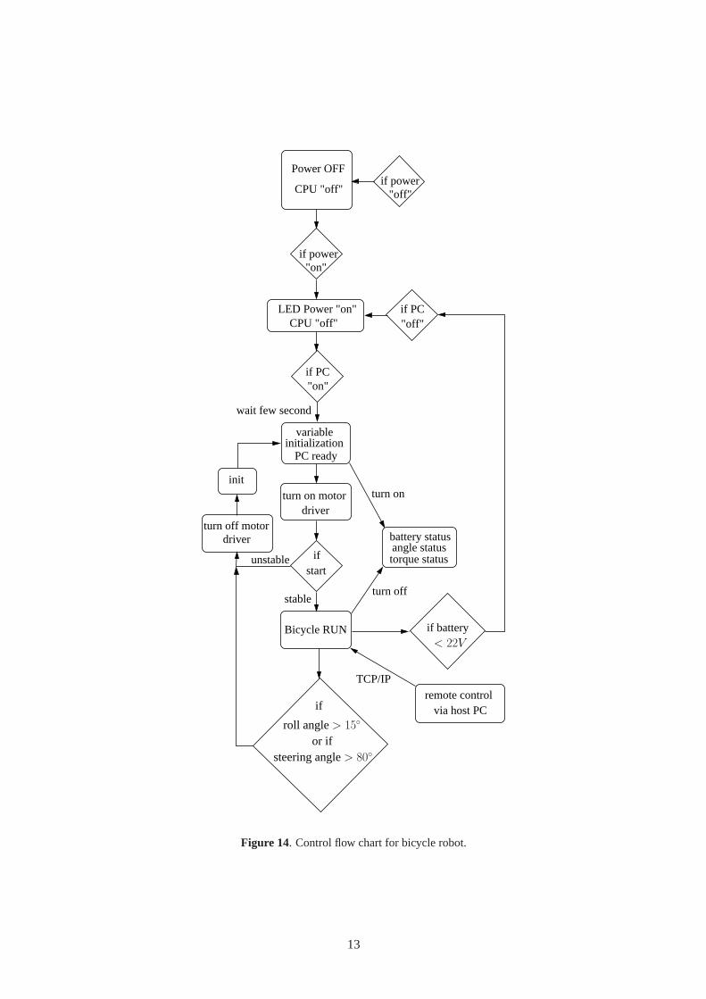
an control flowchart for safety and prevention from the unstable system during the experiment.This flowchart is shown in figure14. The control flowchart for the safety and accident preventionhave been designed to be simple to use. It consists of a power on switch mounted on the panel boxas well as an emergency switch and three switches for enable or disable driver of the motors. Whenturn on pc, the control system will calibrate the sensors. Once the “Ready” light turn on, the usercan simply lift the bicycle and balancer near the upright position. When we push on start button,the bicycle will automatically stabilization at the upright position. In case the bicycle angle islarger than about15◦ or steering angle> 80◦, the control system will automatically switch off thedriver motor. The battery voltage permanently monitor by the control system. Acouple of minutesprior to their being completely discharged, the battery status on the panel will stay turned on thered light. As soon as the batteries reach their minimal voltage, the PC will turn offautomatically.The bicycle robot can be control to move via host PC or via remote control.
5.1 Balancing control of the bicycle robot with balancer
In this experimental study, we perform two different configurations of balancer, first we fix thebalancer length to the COG at maximum lengthhb = 0.14[m] and then we fix the balancer lengthto the COG at the middlehb = 0.07[m]. For the first configuration of the balancer, the controlparameters are setting asa1 = 40, a2 = 15, a3 = 10, a4 = 10. Figure15 shows the roll angleand balancer angle versust. From these results, we can see that the bicycle equilibrium angleis not zero degree that it will make the balancer shift to the reverse side. In the configuration offull length of the balancer, high input torque is required to move the balancer and we need to setthe parametera1 to be large. If we set the parametera1 too large the vibration from the flexible
12
Power OFF
"on"
if PC
if power
"on"
LED Power "on"CPU "off"
CPU "off"if power
"off"
if PC"off"
variable
driverturn on motor
ifstart
wait few second
unstable
driverturn off motor
init
stableturn off
torque status
battery statusangle status
Bicycle RUN
turn on
if battery
remote controlvia host PC
TCP/IP
initializationPC ready
or if
< 22V
if
roll angle> 15◦
steering angle> 80◦
Figure 14. Control flow chart for bicycle robot.
13

0 20 40 60 80 100 120−4
−2
0
2
4
Time [s]
Ang
le [D
egre
e]
(a) Roll angleα
0 20 40 60 80 100 120−40
−20
0
20
40
Time [s]
Ang
le [D
egre
e]
(b) Balancer angleβ
Figure 15. Experimental result of the bicycle stabilization with a balancer mode in full length.
bicycle frame will come out. We need to set an appropriate control parameters depend on thebalancer configuration change. Next the control parameters for the second configuration of thebalancer are setting asa1 = 20, a2 = 12, a3 = 10, a4 = 10. When the length of the balancer toCOG decreased, the parametera1 must be decreased to avoid the vibration from the bicycle frame.The amplitude of the roll angle (Figure16(a)) is also decreased but the balancer moves larger thanthe full length balancer as show in figure16(b).
5.2 Balancing control of the bicycle robot with a flywheel
In this subsection, we use an experimental setup for stabilizing the bicycle withflywheel mode.Figure17 shows the experimental results with the parametersa1 = 38, a2 = 16, a3 = 14 anda4 = 13.
5.3 Field test
In disaster areas, road condition is not so good, because many debris and rubbles are on the roads.Rescue robots need to travel under such condition. To determine how highthe robot can go over,we made this bicycle robot drive on a bumpy road. The bumpy road has bumps from 5 mmto 60 mm high. The bicycle robot could run smoothly. Figure18 shows this test. From theseexperiments, we can see that the bicycle stabilization with flywheel mode worksvery well. Wealso attach the movie of this experimental results.
14

0 10 20 30 40 50 60 70 80 90
−2
−1
0
1
2
Time [s]
Ang
le [D
egre
e]
(a) Roll angleα
0 10 20 30 40 50 60 70 80 90
−40
−20
0
20
40
60
Time [s]
Ang
le [D
egre
e]
(b) Balancer angleβ
Figure 16. Experimental result of the bicycle stabilization with a balancer mode in halflength.
6 Conclusions
The bicycle with balancer model and its balancing control have been presented. A new balancerconfiguration attaches with the bicycle is fully working and we also validated byexperimentalsetup. From the simulation results, the stabilizing bicycle with flywheel has betterperformancethan balancer but it cannot control to shift the bicycle angle to track the desired value, unlikethe balancer which can perform this task. Since the flywheel and the balancer have differentadvantages for stabilizing the bicycle, we used both to stabilize the bicycle. The flywheel is usedwhen the disturbances to the system are large or at startup mode and it will switch to the balancerwhen the system is in the stabilizable region with it. Experimental validation of the stabilizationof the bicycle with the flywheel balancer and the straight running under bumpy road are alsopresented. In the future work, the advantages of balancer mode shouldbe tested in several cases,e.g., turning corners with high speed.
REFERENCES
[1] K. Astrom, R. Klein and A.Lennartsson , “Bicycle Dynamics and Control", IEEE ControlSystem Magazine, 25 (2005), pp. 26-47.
[2] D.J.N. Limebeer and R.S. Sharp , “Bicycles, Motorcycles, and Models,"IEEE Control SystemMagazine, vol. 26, no. 5, pp. 34-61, 2006.
[3] A. L. Schwab, J. P. Meijaard and J. M. Papadopoulos, “Benchmark Results on the LinearizedEquations of Motion of an Uncontrolled Bicycle",KSME International Journal of Mechani-cal Science and Technology, 19 (2005), pp. 292-304.
15

0 10 20 30 40 50 60 70 80−1
−0.5
0
0.5
1
Time [s]
[Deg
ree]
(a) Roll angleα
0 10 20 30 40 50 60 70 80−300
−200
−100
0
100
Time [s]
[Deg
ree]
(b) Balancer angleβ
Figure 17. Bicycle stabilization with the flywheel balancer
[4] R.S. Sharp,“The Stability and Control of Motorcycles,"Journal Mechanical Engineering Sci-ence, vol.13, no. 5, pp.316-329, 1971.
[5] M. Yamakita and A. Utano, “Automatic Control of Bicycle with a Balancer",IEEE/ASME Int.Conf. on Advanced Intelligent Mechatronics., Monterey, California, USA, 2005, pp. 1245-1249.
[6] M. Yamakita, A. Utano and K. Sekiguchi, “Experimental Study of AutomaticControl ofBicycle with Balancer",IEEE/RSJ Int. Conf. on Intelligent Robots and Systems, Beijing,China, 2006, pp. 5606-5611.
[7] A. Murayama and M. Yamakita, “Development of Autonomous Bike Robotwith Balancer",SICE Annual Conference, Kagawa, Japan, 2007, pp. 1048-1052.
[8] L. Keo and M. Yamakita, “Controller Design of an Autonomous Bicycle withBoth Steeringand Balancer Controls,"IEEE Multi-conference on Systems and Control., pp. 1294-1299,2009.
[9] L. Keo and M. Yamakita, “Controlling Balancer and Steering for BicycleStabilization,"IEEE/RSJ Int. Conf. on Intelligent Robots and Systems., pp. 4541-4546, 2009.
[10] A. Okawa, L. Keo and M. Yamakita, “Realization of Acrobatic Turn viaWheelie for a Bi-cycle with a Balancer",Proceeding of IEEE International Conference on Robotics and Au-tomation, Kobe, Japan, 2009 , pp. 2965-2970 .
[11] L. Keo and M. Yamakita, “Control of an Unmanned Electric Bicycle with Flywheel Bal-ancer",Transaction of the Japan Society for Simulation Technology, 2(2010), pp. 32-38.
16

Figure 18. Bicycle test under bumpy road.
[12] J. Yi, D. Song, A. Levandowski and S. Jayasuriya, “Trajectory Tracking and Balance Stabi-lization Control of Autonomous Motorcycle,"Proceeding IEEE Int. conf. on Robotics andAutomation, pp. 2583-2589, 2006.
[13] L. Keo and M. Yamakita, “Dynamic Models of a Bicycle with a Balancer System,"The 26th
annual conference of the Robotics Society of Japan., pp. 43-46, 2008.
[14] L. Keo and M. Yamakita, “Trajectory Control for an Autonomous Bicycle with Balancer,"IEEE/ASME Int. Conf. on Ad. Intel. Mechatronics., pp. 676-681, 2008.
[15] N.H. Getz, “Dynamic Inversion of Nonlinear Maps with Applications to Nonlinear Controland Robotics,"Ph.D dissertation, Department of Electrical Engineering and Computer Sci-ences, University of California at Berkeley, CA, 1995.
[16] N.H. Getz , J.E. Marsden , “Control for an Autonomous Bicycle,"Proceeding IEEE Int. conf.on Robotics and Automation, pp. 1397-1402, 1995.
17