Dynamic Logic for Plan Revision inIntelligent Agents

M. Birna van Riemsdijk

Frank S. de Boer

John-Jules Ch. Meyer

institute of information and computing sciences,utrecht university

technical report UU-CS-2005-013

www.cs.uu.nl

Dynamic Logic for Plan Revision in IntelligentAgents

M. Birna van Riemsdijk1 Frank S. de Boer1,2,3 John-Jules Ch. Meyer1

1 ICS, Utrecht University, The Netherlands2 CWI, Amsterdam, The Netherlands

3 LIACS, Leiden University, The Netherlands

Abstract. In this paper, we present a dynamic logic for a propositionalversion of the agent programming language 3APL. A 3APL agent hasbeliefs and a plan. The execution of a plan changes an agent’s beliefs.Plans can be revised during execution. Due to these plan revision capa-bilities of 3APL agents, plans cannot be analyzed by structural inductionas in for example standard propositional dynamic logic. We propose adynamic logic that is tailored to handle the plan revision aspect of 3APL.For this logic, we give a sound and complete axiomatization.

1 Introduction

An agent is commonly seen as an encapsulated computer system that is situatedin some environment and that is capable of flexible, autonomous action in thatenvironment in order to meet its design objectives [23]. Programming these flex-ible computing entities is not a trivial task. An important line of research in thisarea, is research on cognitive agents. These are agents endowed with high-levelmental attitudes such as beliefs, desires, goals, plans, intentions, norms and obli-gations. Intelligent cognitive agents should be able to reason with these mentalattitudes in order to exhibit the desired flexible problem solving behavior.

The very concept of (cognitive) agents is thus a complex one. It is imper-ative that programmed agents be amenable to precise and formal specificationand verification, at least for some critical applications. This is recognized by(potential) appliers of agent technology such as NASA, which organizes special-ized workshops on the subject of formal specification and verification of agents[16,11].

In this paper, we are concerned with the verification of agents programmedin (a simplified version of) the cognitive agent programming language 3APL4

[12,22,5]. This language is based on theoretical research on cognitive notions[3,4,15,18]. In the latest version [5], a 3APL agent has a set of beliefs, a planand a set of goals. The idea is that an agent tries to fulfill its goals by selectingappropriate plans, depending on its beliefs about the world. Beliefs should thusrepresent the world or environment of the agent; the goals represent the state of

4 3APL is to be pronounced as “triple-a-p-l”.

the world the agent wants to realize and plans are the means to achieve thesegoals.

As explained, cognitive agent programming languages are designed to pro-gram flexible behavior using high-level mental attitudes. In the various lan-guages, these attitudes are handled in different ways. An important aspect of3APL is the way in which plans are dealt with. A plan in 3APL can be executed,resulting in a change of the beliefs of the agent.5 Now, in order to increase thepossible flexibility of agents, 3APL [12] was endowed with a mechanism withwhich the programmer can program agents that can revise their plans duringexecution of the agent. This is a distinguishing feature of 3APL compared toother agent programming languages and architectures [14,17,8,7]. The idea isthat an agent should not blindly execute an adopted plan, but it should be ableto revise it under certain conditions. As this paper focusses on the plan revi-sion aspect of 3APL, we consider a version of the language with only beliefsand plans, i.e., without goals. We will use a propositional and otherwise slightlysimplified variant of the original 3APL language as defined in [12].

In 3APL, the plan revision capabilities can be programmed through planrevision rules. These rules consist of a head and a body, both representing aplan. A plan is basically a sequence of so-called basic actions. These actions canbe executed. The idea is, informally, that an agent can apply a rule if it has a plancorresponding to the head of this rule, resulting in the replacement of this planby the plan in the body of the rule. The introduction of these capabilities nowgives rise to interesting issues concerning the characteristics of plan execution,as will become clear in the sequel. This has implications for reasoning about theresult of plan execution and therefore for the formal verification of 3APL agents,which we are concerned with in this paper.

As for related work, verification of agents programmed in an agent program-ming language has for example been addressed in [2]. This paper addresses modelchecking of the agent programming language AgentSpeak. A sketch of a dynamiclogic to reason about 3APL agents has been given in [22]. This logic however isdesigned to reason about a 3APL interpreter or deliberation language, whereasin this paper we take a different viewpoint and reason about plans. In [13], aprogramming logic (without axiomatization) was given for a fragment of 3APLwithout plan revision rules. Further, the operational semantics of plan revisionrules is similar to that of procedures in procedural programming. In fact, planrevision rules can be viewed as an extension of procedures. Logics and semanticsfor procedural languages are for example studied in De Bakker [6]. Although theoperational semantics of procedures and plan revision rules are similar, tech-niques for reasoning about procedures cannot be used for plan revision rules.This is due to the fact that the introduction of these rules results in the seman-tics of the sequential composition operator no longer being compositional (seesections 3 and 6). This issue has also been considered from a semantic perspectivein [21].

5 A change in the environment is a possible “side effect” of the execution of a plan.

3

The outline of the paper is as follows. After defining (a simplified versionof) 3APL and its semantics (section 2), we propose a dynamic logic for prov-ing properties of 3APL plans in the context of plan revision rules (section 3).As will become clear, this is actually not a logic for general 3APL plans, butthe plans that the logic can deal with are restricted in a certain way. For thislogic, we provide a sound and complete axiomatization (section 4). In section5, we discuss how this logic for restricted 3APL plans can be extended to alogic for non-restricted plans and we discuss some example proofs, using thelogic. Finally, we consider the relation between proving properties of proceduralprograms and proving properties of 3APL agents in section 6. In particular, wecompare procedures with plan revision rules.

To the best of our knowledge, this is the first attempt to design a logicand deductive system for plan revision rules or similar language constructs.6

Considering the semantic difficulties that arise with the introduction of this typeof construct, it is not a priori obvious that it would be possible at all to designa deductive system to reason about these constructs. The main aim of this workwas thus to investigate whether it is possible to define such a system, and inthis way also to get a better theoretical understanding of the construct of planrevision rules. Whether the system presented in this paper is also practicallyuseful to verify 3APL agents, remains to be seen and will be subject to furtherresearch.

2 3APL

2.1 Syntax

Below, we define belief bases and plans. A belief base is a set of propositionalformulas. A plan is a sequence of basic actions and abstract plans. Basic actionscan be executed, resulting in a change to the beliefs of the agent. An abstractplan can, in contrast with basic actions, not be executed directly in the sensethat it updates the belief base of an agent. Abstract plans serve as an abstractionmechanism like procedures in procedural programming. If a plan consists of anabstract plan, this abstract plan could be transformed into basic actions throughthe application of plan revision rules, which will be introduced below.7

In the sequel, a language defined by inclusion shall be the smallest languagecontaining the specified elements.

Definition 1 (belief bases) Assume a propositional language L with typicalformula p and the connectives ∧ and ¬ with the usual meaning. Then the set ofbelief bases Σ with typical element σ is defined to be ℘(L).8

6 Parts of this work have been published in [20].7 Abstract plans could also be modelled as non-executable basic actions.8 ℘(L) denotes the powerset of L.

4

Definition 2 (plans) Assume that a set BasicAction with typical element a isgiven, together with a set AbstractPlan with typical element p.9 Then the set ofplans Plan with typical element π is defined as follows:

– BasicAction ∪ AbstractPlan ⊆ Plan,– if c ∈ (BasicAction ∪ AbstractPlan) and π ∈ Plan then c ;π ∈ Plan.

Basic actions and abstract plans are called atomic plans and are typically de-noted by c. For technical convenience, plans are defined to have a list structure,which means, strictly speaking, that we can only use the sequential compositionoperator to concatenate an atomic plan and a plan, rather than concatenatingtwo arbitrary plans. In the following, we will however also use the sequentialcomposition operator to concatenate arbitrary plans π1 and π2 yielding π1;π2.The operator should in this case be read as a function taking two plans thathave a list structure and yielding a new plan that also has this structure. Theplan π1 will thus be the prefix of the resulting plan.

We use ε to denote the empty plan, which is an empty list. The concatenationof a plan π and the empty list is equal to π, i.e., ε;π and π; ε are identified withπ.

A plan and a belief base can together constitute a so-called configuration.During computation or execution of the agent, the elements in a configurationcan change.

Definition 3 (configuration) Let Σ be the set of belief bases and let Plan bethe set of plans. Then Plan×Σ is the set of configurations of a 3APL agent.

Plan revision rules consist of a head πh and a body πb. Informally, an agent thathas a plan πh, can replace this plan by πb when applying a plan revision rule ofthis form.

Definition 4 (plan revision (PR) rules) The set of PR rules R is defined asfollows: R = πh πb | πh, πb ∈ Plan, πh 6= ε.10

Take for example a plan a; b where a and b are basic actions, and a PR rulea; b c. The agent can then either execute the actions a and b one after theother, or it can apply the PR rule yielding a new plan c, which can in turn beexecuted. A plan p consisting of an abstract plan cannot be executed, but canonly be transformed using a procedure-like PR rule such as p a.

Below, we provide the definition of a 3APL agent. The function T , taking abasic action and a belief base and yielding a new belief base, is used to definehow belief bases are updated when a basic action is executed.9 Note that we use p to denote an element from the propositional language L, as well

as an element from AbstractPlan. It will however be indicated explicitly which kindof element is meant.

10 In [12], PR rules were defined to have a guard, i.e., rules were of the form πh | φ πb.For a rule to be applicable, the guard should then hold. For technical convenienceand because we want to focus on the plan revision aspect of these rules, we howeverleave out the guard in this paper.

5

Definition 5 (3APL agent) A 3APL agent A is a tuple〈Rule, T 〉 where Rule ⊆ R is a finite set of PR rules and T : (BasicAction×Σ) →Σ is a partial function, expressing how belief bases are updated through basicaction execution.

2.2 Semantics

The semantics of a programming language can be defined as a function taking astatement and a state, and yielding the set of states resulting from executing theinitial statement in the initial state. In this way, a statement can be viewed asa transformation function on states. In 3APL, plans can be seen as statementsand belief bases as states on which these plans operate. There are various waysof defining a semantic function and in this paper we are concerned with theso-called operational semantics (see for example De Bakker [6] for details on thissubject).

The operational semantics of a language is usually defined using transitionsystems [?]. A transition system for a programming language consists of a set ofaxioms and derivation rules for deriving transitions for this language. A transi-tion is a transformation of one configuration into another and it corresponds to asingle computation step. Let A = 〈Rule, T 〉 be a 3APL agent and let BasicActionbe a set of basic actions. Below, we give the transition system TransA for oursimplified 3APL language, which is based on the system given in [12]. This tran-sition system is specific to agent A.

There are two kinds of transitions, i.e., transitions describing the executionof basic actions and those describing the application of a plan revision rule. Thetransitions are labelled to denote the kind of transition. A basic action at thehead of a plan can be executed in a configuration if the function T is defined forthis action and the belief base in the configuration. The execution results in achange of belief base as specified through T and the action is removed from theplan.

Definition 6 (action execution) Let a ∈ BasicAction.

T (a, σ) = σ′

〈a;π, σ〉 →exec 〈π, σ′〉

A plan revision rule can be applied in a configuration if the head of the rule isequal to a prefix of the plan in the configuration. The application of the ruleresults in the revision of the plan, such that the prefix equal to the head of therule is replaced by the plan in the body of the rule. A rule a; b c can forexample be applied to the plan a; b; c, yielding the plan c; c. The belief base isnot changed through plan revision.

Definition 7 (rule application) Let ρ : πh πb ∈ Rule.

〈πh;π, σ〉 →app 〈πb;π, σ〉

6

In the sequel, it will be useful to have a function taking a PR rule and a plan,and yielding the plan resulting from the application of the rule to this givenplan. Based on this function, we also define a function taking a set of PR rulesand a plan and yielding the set of rules applicable to this plan.

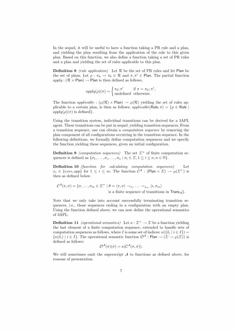
Definition 8 (rule application) Let R be the set of PR rules and let Plan bethe set of plans. Let ρ : πh πb ∈ R and π, π′ ∈ Plan. The partial functionapply : (R× Plan) → Plan is then defined as follows.

apply(ρ)(π) =πb;π′ if π = πh;π′,undefined otherwise.

The function applicable : (℘(R) × Plan) → ℘(R) yielding the set of rules ap-plicable to a certain plan, is then as follows: applicable(Rule, π) = ρ ∈ Rule |apply(ρ)(π) is defined.

Using the transition system, individual transitions can be derived for a 3APLagent. These transitions can be put in sequel, yielding transition sequences. Froma transition sequence, one can obtain a computation sequence by removing theplan component of all configurations occurring in the transition sequence. In thefollowing definitions, we formally define computation sequences and we specifythe function yielding these sequences, given an initial configuration.

Definition 9 (computation sequences) The set Σ+ of finite computation se-quences is defined as σ1, . . . , σi, . . . , σn | σi ∈ Σ, 1 ≤ i ≤ n, n ∈ N.

Definition 10 (function for calculating computation sequences) Letxi ∈ exec, app for 1 ≤ i ≤ m. The function CA : (Plan × Σ) → ℘(Σ+) isthen as defined below.

CA(π, σ) = σ, . . . , σm ∈ Σ+ | θ = 〈π, σ〉 →x1 . . .→xm〈ε, σm〉

is a finite sequence of transitions in TransA.

Note that we only take into account successfully terminating transition se-quences, i.e., those sequences ending in a configuration with an empty plan.Using the function defined above, we can now define the operational semanticsof 3APL.

Definition 11 (operational semantics) Let κ : Σ+ → Σ be a function yieldingthe last element of a finite computation sequence, extended to handle sets ofcomputation sequences as follows, where I is some set of indices: κ(δi | i ∈ I) =κ(δi) | i ∈ I. The operational semantic function OA : Plan → (Σ → ℘(Σ)) isdefined as follows:

OA(π)(σ) = κ(CA(π, σ)).

We will sometimes omit the superscript A to functions as defined above, forreasons of presentation.

7

Example 1 Let A be an agent with PR rules p; a b, p c, where p isan abstract plan and a, b, c are basic actions. Let σa be the belief base resultingfrom the execution of a in σ, i.e., T (a, σ) = σa, let be σab the belief resultingfrom executing first a and then b in σ, etc.

Then CA(p; a)(σ) = (σ, σ, σb), (σ, σ, σc, σca), which is based on the transi-tion sequences 〈p; a, σ〉 →app 〈b, σ〉 →exec 〈ε, σb〉 and 〈p; a, σ〉 →app 〈c; a, σ〉 →exec

〈a, σc〉 →exec 〈ε, σca〉. We thus have that OA(p; a)(σ) = σb, σca. 4

3 Plan Revision Dynamic Logic

In programming language research, an important area is the specification andverification of programs. Program logics are designed to facilitate this process.One such logic is dynamic logic [9,10], with which we are concerned in this paper.In dynamic logic, programs are explicit syntactic constructs in the logic. To beable to discuss the effect of the execution of a program π on the truth of aformula φ, the modal construct [π]φ is used. This construct intuitively statesthat in all states in which π halts, the formula φ holds.

Programs in general are constructed from atomic programs and compositionoperators. An example of a composition operator is the sequential compositionoperator (;), where the program π1;π2 intuitively means that π1 is executed first,followed by the execution of π2. The semantics of such a compound program canin general be determined by the semantics of the parts of which it is composed.This compositionality property allows analysis by structural induction (see also[19]), i.e., analysis of a compound statement by analysis of its parts. Analysis ofthe sequential composition operator by structural induction can in dynamic logicbe expressed by the following formula, which is usually a validity: [π1;π2]φ ↔[π1][π2]φ. For 3APL plans on the contrary, this formula does not always hold.This is due to the presence of PR rules.

We will informally explain this using the 3APL agent of example 1. As ex-plained, the operational semantics of this agent, given initial plan p; a and initialstate σ, is as follows: O(p; a)(σ) = σb, σca. Now compare the result of first “ex-ecuting”11 p in σ and then executing a in the resulting belief base, i.e., comparethe set O(a)(O(p)(σ)). In this case, there is only one successfully terminatingtransition sequence and it ends in σca, i.e., O(a)(O(p)(σ)) = σca. Now, if itwould be the case that σca |= φ but σb 6|= φ, the formula [p; a]φ↔ [p][a]φ wouldnot hold.12

Analysis of plans by structural induction in this way thus does not work for3APL. In order to be able to prove correctness properties of 3APL programshowever, one can perhaps imagine that it is important to have some kind of11 We will use the word “execution” in two ways. Firstly, as in this context, we will use

it to denote the execution of an arbitrary plan in the sense of going through severaltransition of type exec or app, starting in a configuration with this plan and resultingin some final configurations. Secondly, we will use it to refer to the execution of abasic action in the sense of going through a transition of type exec.

12 In particular, the implication would not hold from right to left.

8

induction. As we will show in the sequel, the kind of induction that can beused to reason about 3APL programs, is induction on the number of PR ruleapplications in a transition sequence. We will introduce a dynamic logic for 3APLbased on this idea.

3.1 Syntax

In order to be able to do induction on the number of PR rule applications ina transition sequence, we introduce so-called restricted plans. These are plans,annotated with a natural number13. Informally, if the restriction parameter of aplan is n, the number of rule applications during execution of this plan cannotexceed n.

Definition 12 (restricted plans) Let Plan be the language of plans and letN− = N ∪ −1. Then, the language Planr of restricted plans is defined asπn | π ∈ Plan, n ∈ N−.

Below, we define the language of dynamic logic in which properties of 3APLagents can be expressed. In the logic, one can express properties of restrictedplans. As will become clear in the sequel, one can prove properties of the planof a 3APL agent by proving properties of restricted plans.

Definition 13 (plan revision dynamic logic (PRDL)) Let π n∈ Planr be arestricted plan and let A be a 3APL agent (definition 5). Then the language ofdynamic logic LPRDL with typical element φ is defined as follows:

– L ⊆ LPRDL,– if φ ∈ LPRDL, then [πn]φ ∈ LPRDL,– if φ, φ′ ∈ LPRDL, then ¬φ ∈ LPRDL and φ ∧ φ′ ∈ LPRDL.

3.2 Semantics

In order to define the semantics of PRDL, we first define the semantics of re-stricted plans. As for ordinary plans, we also define an operational semantics forrestricted plans. We do this by defining a function for calculating computationsequences, given an initial restricted plan and a belief base.

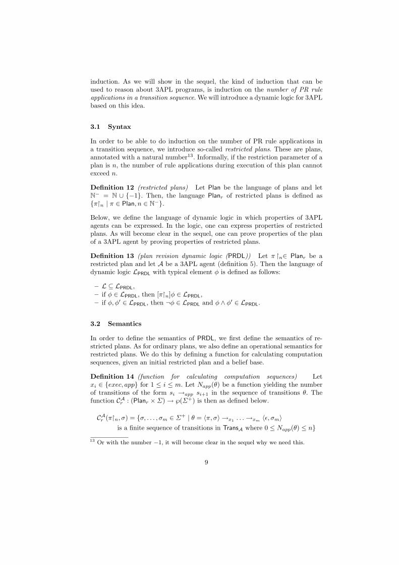
Definition 14 (function for calculating computation sequences) Letxi ∈ exec, app for 1 ≤ i ≤ m. Let Napp(θ) be a function yielding the numberof transitions of the form si →app si+1 in the sequence of transitions θ. Thefunction CAr : (Planr ×Σ) → ℘(Σ+) is then as defined below.

CAr (πn, σ) = σ, . . . , σm ∈ Σ+ | θ = 〈π, σ〉 →x1 . . .→xm〈ε, σm〉

is a finite sequence of transitions in TransA where 0 ≤ Napp(θ) ≤ n

13 Or with the number −1, it will become clear in the sequel why we need this.

9

As one can see in the definition above, the computation sequences CAr (πn, σ)are based on transition sequences starting in configuration 〈π, σ〉. The numberof rule applications in these transition sequences should be between 0 and n, incontrast with the function CA of definition 10, in which there is no restrictionon this number.

Based on the function CAr , we define the operational semantics of restrictedplans by taking the last elements of the computation sequences yielded by CAr .The set of belief bases is empty if the restriction parameter is equal to −1.

Definition 15 (operational semantics) Let κ be as in definition 11. The oper-ational semantic function OA

r : Planr → (Σ → ℘(Σ)) is defined as follows:

OAr (πn)(σ) =

κ(CAr (πn, σ)) if n ≥ 0,∅ if n = −1.

Using the operational semantics of restricted plans, we can now define the se-mantics of plan revision dynamic logic.

Definition 16 (semantics of PRDL) Let p ∈ L be a propositional formula, letφ, φ′ ∈ LPRDL and let |=L be the entailment relation defined for L as usual. Thesemantics |=A of LPRDL is then as defined below.

σ |=A p ⇔ σ |=L pσ |=A [πn]φ⇔ ∀σ′ ∈ OA

r (πn)(σ) : σ′ |=A φσ |=A ¬φ ⇔ σ 6|=A φσ |=A φ ∧ φ′ ⇔ σ |=A φ and σ |=A φ′

As OAr is defined in terms of agent A, so is the semantics of LPRDL. We use

the subscript A to indicate this. Let Rule ⊆ R be a finite set of PR rules. If∀T , σ : σ |=〈Rule,T 〉 φ, we write |=Rule φ.

4 The Axiom System

In order to prove properties of restricted plans, we propose a deductive systemfor PRDL in this section. Rather than proving properties of restricted plans, theaim is however to prove properties of non-restricted 3APL plans. The idea isthat this can be done using the axiom system for restricted plans, by relatingthe semantics of restricted plans to that of non-restricted plans. We will explainand elaborate on this in section 5.

Definition 17 (axiom system (ASRule)) Let BasicAction be a set of basic ac-tions, AbstractPlan be a set of abstract plans and Rule ⊆ R be a finite set ofPR rules. Let a ∈ BasicAction, let p ∈ AbstractPlan, let c ∈ (BasicAction ∪AbstractPlan) and let ρ range over applicable(Rule, c;π). The following are then

10

the axioms of the system ASRule.

(PRDL1) [π−1]φ(PRDL2) [p0]φ(PRDL3) [εn]φ↔ φ with 0 ≤ n(PRDL4) [c;πn]φ↔ [c0][πn]φ ∧

∧ρ[apply(ρ, c;π)n−1]φ with 0 ≤ n

(PL) axioms for propositional logic(PDL) [πn](φ→ φ′) → ([πn]φ→ [πn]φ′)

The following are the rules of the system ASRule.

(GEN)φ

[πn]φ

(MP)φ1, φ1 → φ2

φ2

As the axiom system is relative to a given set of PR rules Rule, we will use thenotation `Rule φ to specify that φ is derivable in the system ASRule above.

We will now explain the PRDL axioms of the system. The other axioms andthe rules are standard for propositional dynamic logic (PDL) [9]. We start byexplaining the most interesting axiom: (PRDL4). We first observe that there aretwo types of transitions that can be derived for a 3APL agent: action executionand rule application (see definitions 6 and 7). Consider a configuration 〈a;π, σ〉where a is a basic action. Then during computation, possible next configurationsare 〈π, σ′〉14 (action execution) and 〈apply(ρ, a;π), σ〉 (rule application) where ρranges over the applicable rules, i.e., applicable(Rule, a;π).15 We can thus analyzethe plan a;π by analyzing π after the execution of a, and the plans resultingfrom applying a rule, i.e., apply(ρ, a;π).16 The execution of an action can berepresented by the number 0 as restriction parameter, yielding the first term ofthe right-hand side of (PRDL4): [a0][πn]φ.17 The second term is a conjunctionof [apply(ρ, c;π)n−1]φ over all applicable rules ρ. The restriction parameter isn−1 as we have “used” one of our n permitted rule applications. The first threeaxioms represent basic properties of restricted plans. (PRDL1) can be used toeliminate the second term on the right-hand side of axiom (PRDL4), if the left-hand side is [c;π0]φ. (PRDL2) can be used to eliminate the first term on theright-hand side of (PRDL4), if c is an abstract plan. As abstract plans can onlybe transformed through rule application, there will be no resulting states if the

14 assuming that T (a, σ) = σ′15 See definition 8 for the definitions of the functions apply and applicable.16 Note that one could say we analyze a plan a; π partly by structural induction, as it

is partly analyzed in terms of a and π.17 In our explanation, we consider the case where c is a basic action, but the axiom

holds also for abstract plans.

11

restriction parameter of the abstract plan is 0, i.e., if no rule applications areallowed. (PRDL3) states that if φ is to hold after execution of the empty plan, itshould hold “now”. It can be used to derive properties of an atomic plan c, byusing axiom (PRDL4) with the plan c; ε.

4.1 Soundness

The axiom system of definition 17 is sound.

Theorem 1 (soundness) Let φ ∈ LPRDL. Let Rule ⊆ R be an arbitrary finiteset of PR rules. Then the axiom system ASRule is sound, i.e.:

`Rule φ ⇒ |=Rule φ.

Proof: We prove soundness of the PRDL axioms of the system ASRule. In thefollowing, let π ∈ Plan be an arbitrary plan and let φ ∈ LPRDL be an arbitraryPRDL formula. Furthermore, A = 〈Rule, T 〉 and |=〈Rule,T 〉 will be abbreviatedby |=Rule.

(PRDL1) To prove: ∀T , σ : σ |=Rule [π −1]φ. Let σ ∈ Σ be an arbitrarybelief base and let T be an arbitrary belief update function. We have thatσ |=Rule [π −1]φ ⇔ ∀σ′ ∈ OA

r (π −1)(σ) : σ′ |=Rule φ by definition 16. Fur-thermore, OA

r (π−1)(σ) = ∅ by definition 15, trivially yielding the desired result.

(PRDL2) Let p ∈ AbstractPlan be an arbitrary abstract plan. Toprove: ∀T , σ : σ |=Rule [p 0]φ. Let σ ∈ Σ be an arbitrary beliefbase and let T be an arbitrary belief update function. We have thatσ |=Rule [p 0]φ ⇔ ∀σ′ ∈ OA

r (p 0)(σ) : σ′ |=Rule φ by definition 16. Further-more, OA

r (p 0)(σ) = ∅ by definition 6, trivially yielding the desired result.

(PRDL3) To prove: ∀T , σ : σ |=Rule [ε n]φ ↔ φ where n ≥ 0, i.e.,∀T , σ : (σ |=Rule [ε n]φ ⇔ σ |=Rule φ). Let σ ∈ Σ be an arbitrary beliefbase and let T be an arbitrary belief update function. By definition 14, we havethat CAr (εn, σ) = σ where n ≥ 0, i.e.:

κ(CAr (εn, σ)) = σ. (4.1)

By definitions 16, 15 and (4.1), we have the following, yielding the desired result.

σ |=Rule [εn]φ⇔ ∀σ′ ∈ OAr (εn)(σ) : σ′ |=Rule φ

⇔ ∀σ′ ∈ κ(CAr (εn, σ)) : σ′ |=Rule φ⇔ σ |=Rule φ

(PRDL4) To prove: ∀T , σ : σ |=〈Rule,T 〉 [c;π n]φ ↔ [c 0][π n]φ ∧

∧ρ[apply(ρ, c;π)n−1]φ, i.e.:

∀T , σ : σ |=〈Rule,T 〉 [c;πn]φ⇔ ∀T , σ : σ |=〈Rule,T 〉 [c0][πn]φ and

∀T , σ : σ |=〈Rule,T 〉∧ρ

[apply(ρ, c;π)n−1]φ.

12

Let σ ∈ Σ be an arbitrary belief base and let T be an arbitrary belief updatefunction. Assume c ∈ BasicAction and furthermore assume that 〈c;π, σ〉 →execute

〈π, σ1〉 is a transition in TransA, i.e., κ(CAr (c0, σ)) = σ1 by definition 14. Letρ range over applicable(Rule, c;π). Now, observe the following by definition 14:

κ(CAr (c;πn, σ)) = κ(CAr (πn, σ1)) ∪⋃ρ

κ(CAr (apply(ρ, c;π)n−1, σ)). (4.2)

If c ∈ AbstractPlan or if a transition of the form 〈c;π, σ〉 →execute 〈π, σ1〉 is notderivable, the first term of the right-hand side of (4.2) is empty.

(⇒) Assume σ |=Rule [c;π n]φ, i.e., by definition 16 ∀σ′ ∈ OAr (c;π n, σ) :

σ′ |=Rule φ, i.e., by definition 15:

∀σ′ ∈ κ(CAr (c;πn, σ)) : σ′ |=Rule φ. (4.3)

To prove: (A) σ |=Rule [c0][πn]φ and (B) σ |=Rule

∧ρ[apply(ρ, c;π)n−1]φ.

(A) If c ∈ AbstractPlan or if a transition of the form 〈c;π, σ〉 →execute 〈π, σ1〉 isnot derivable, the desired result follows immediately from axiom (PRDL2) or ananalogous proposition for non executable basic actions. If c ∈ BasicAction, wehave the following from definitions 16 and 15.

σ |=Rule [c0][πn]φ⇔ ∀σ′ ∈ OAr (c0, σ) : σ′ |=Rule [πn]φ

⇔ ∀σ′ ∈ OAr (c0, σ) : ∀σ′′ ∈ OA

r (πn, σ′) : σ′′ |=Rule φ⇔ ∀σ′ ∈ κ(CAr (c0, σ)) : ∀σ′′ ∈ κ(CAr (πn, σ′)) : σ′′ |=Rule φ⇔ ∀σ′′ ∈ κ(CAr (πn, σ1)) : σ′′ |=Rule φ

(4.4)

From 4.2, we have that κ(CAr (π n, σ1)) ⊆ κ(CAr (c;π n, σ)). From this andassumption (4.3), we can now conclude the desired result (4.4).

(B) Let c ∈ (BasicAction ∪ AbstractPlan) and let ρ ∈ applicable(Rule, c;π). Thenwe want to prove σ |=Rule [apply(ρ, c;π)n−1]φ. From definitions 16 and 15, wehave the following.

σ |=Rule [apply(ρ, c;π)n−1]φ⇔ ∀σ′ ∈ OAr (apply(ρ, c;π)n−1, σ) : σ′ |=Rule φ

⇔ ∀σ′ ∈ κ(CAr (apply(ρ, c;π)n−1, σ)) : σ′ |=Rule φ

(4.5)

From 4.2, we have that κ(CAr (apply(ρ, c;π)n−1, σ)) ⊆ κ(CAr (c;π n, σ)). Fromthis and assumption (4.3), we can now conclude the desired result (4.5).

(⇐) Assume σ |=Rule [c 0][π n]φ and σ |=Rule

∧ρ[apply(ρ, c;π) n−1]φ, i.e.,

∀σ′ ∈ κ(CAr (πn, σ1)) : σ′ |=Rule φ (4.4) and ∀σ′ ∈ κ(CAr (apply(ρ, c;π)n−1, σ)) :σ′ |=Rule φ (4.5).To prove: σ |=Rule [c;π n]φ, i.e., ∀σ′ ∈ κ(CAr (c;π n, σ)) : σ′ |=Rule φ (4.3). Ifc ∈ AbstractPlan or if a transition of the form 〈c;π, σ〉 →execute 〈π, σ1〉 is not

13

derivable, we have that κ(CAr (c;πn, σ)) =⋃

ρ κ(CAr (apply(ρ, c;π)n−1, σ)) (4.2).From this and the assumption, we have the desired result.

If c ∈ BasicAction and a transition of the form 〈c;π, σ〉 →execute 〈π, σ1〉 isderivable, we have (4.2). From this and the assumption, we again have the desiredresult. 2

4.2 Completeness

In order to prove completeness of the axiom system, we first prove proposition1, which says that any formula from LPRDL can be rewritten into an equivalentformula where all restriction parameters are 0. This proposition is proven byinduction on the size of formulas. The size of a formula is defined by means ofthe function size : LPRDL → N3. This function takes a formula from LPRDL andyields a triple 〈x, y, z〉, where x roughly corresponds to the sum of the restrictionparameters occurring in the formula, y roughly corresponds to the sum of thelength of plans in the formula and z is the length of the formula.

Definition 18 (size) Let the following be a lexicographic ordering on tuples〈x, y, z〉 ∈ N3:

〈x1, y1, z1〉 < 〈x2, y2, z2〉 iffx1 < x2 or (x1 = x2 and y1 < y2) or (x1 = x2 and y1 = y2 and z1 < z2).

Let max be a function yielding the maximum of two tuples from N3 and let fand s respectively be functions yielding the first and second element of a tuple.Let l be a function yielding the number of symbols of a syntactic entity and letl(ε) = 0. The function size : LPRDL → N3 is then as defined below.

size(p) = 〈0, 0, l(p)〉

size([πn]φ) =〈n+ f(size(φ)), l(π) + s(size(φ)), l([πn]φ)〉 if n > 0〈f(size(φ)), s(size(φ)), l([πn]φ)〉 otherwise

size(¬φ) = 〈f(size(φ)), s(size(φ)), l(¬φ)〉size(φ ∧ φ′) = 〈f(max(size(φ), size(φ′))), s(max(size(φ), size(φ′))), l(φ ∧ φ′)〉

Note that when calculating the plan length of a formula [π n]φ, i.e., the sec-ond element of the tuple size([πn]φ), the length of π is added to the lengthof the plans in φ in case n > 0. If however n = 0 or n = −1, the lengthof π is not added to the length of the plans in φ and s(size(φ)) is simplyreturned. This definition of the function size results in the fact that a for-mula φ in which all restriction parameters are 0 (or −1), will satisfy size(φ) =〈0, 0, l(φ)〉. Further, this definition gives us that size([c0][πn]φ) is smaller thansize([c;πn]φ), which is needed in the proof of lemma 1, which will be used inthe proof of proposition 1.

Clause (4.7) of lemma 1 specifies that the right-hand side of axiom (PRDL4)is smaller than the left-hand side. This axiom will usually be used by applyingit from left to right to prove a formula such as [πn]φ. Intuitively, the fact that

14

the formula will get “smaller” as specified through the function size, suggestsconvergence of the deduction process.

Lemma 1 Let φ ∈ LPRDL, let c ∈ (BasicAction ∪ AbstractPlan), let ρ rangeover applicable(Rule, c;π) and let n > 0. The following then holds.

size(φ) < size([εn]φ) (4.6)

size([c0][πn]φ ∧∧ρ

[apply(ρ, c;π)n−1]φ) < size([c;πn]φ) (4.7)

size(φ) < size(φ ∧ φ′) (4.8)size(φ′) < size(φ ∧ φ′) (4.9)

Proof: First, we prove (4.6). From definition 18, we have:

size([εn]φ) = 〈n+ f(size(φ)), s(size(φ)), l([εn]φ)〉.

This is bigger than size(φ).Now we prove (4.7). We have the following from definition 18, using that

n > 0:

size([c;πn]φ) = 〈n+ f(size(φ)), l(c;π) + s(size(φ)), l([c;πn]φ)〉,size([c0][πn]φ) = 〈n+ f(size(φ)), l(π) + s(size(φ)), l([c0][πn]φ)〉,size([apply(ρ, c;π)n−1]φ) = 〈(n− 1) + f(size(φ)), l(apply(ρ, c;π))

+s(size(φ)), l([apply(ρ, c;π)n−1]φ)〉.

Let F = [c 0][π n]φ and S = [apply(ρ, c;π) n−1]φ. Then,max(size(F ), size(S)) = size(F ) for any PR rule ρ. Thus, size(F ∧

∧ρ S) =

〈n+f(size(φ)), l(π)+s(size(φ)), l(F ∧∧

ρ S)〉, which is smaller than size([c;πn]φ), yielding the desired result.

Finally, we prove (4.8) and (4.9). First, we show that size(φ) < size(φ∧φ′),which we will refer to by R. We thus have to show:

〈f(size(φ)), s(size(φ)), l(φ)〉 <〈f(max(size(φ), size(φ′))), s(max(size(φ), size(φ′))), l(φ ∧ φ′)〉.

If f(size(φ)) < f(max(size(φ), size(φ′))), we have R. If f(size(φ)) =f(max(size(φ), size(φ′))) and s(size(φ)) < s(max(size(φ), size(φ′))), we againhave R. If s(size(φ)) = s(max(size(φ), size(φ′))), we also have R, becausel(φ) < l(φ ∧ φ′). Covering all cases, this yields the desired result. The sameline of reasoning can be applied to show size(φ′) < size(φ ∧ φ′). 2

Now we can formulate and prove the following proposition.

Proposition 1 Any formula φ ∈ LPRDL can be rewritten into an equivalentformula φPDL where all restriction parameters are 0, i.e.:

∀φ ∈ LPRDL : ∃φPDL ∈ LPRDL : size(φPDL) = 〈0, 0, l(φPDL)〉 and `Rule φ↔ φPDL.

15

Proof: The fact that a formula φ has the property that it can be rewrittenas specified in the proposition, will be denoted by PDL(φ) for reasons that willbecome clear in the sequel. The proof is by induction on size(φ).

– φ ≡ psize(p) = 〈0, 0, l(p)〉 and let pPDL = p, then PDL(p).

– φ ≡ [πn]φ′

If n = −1, we have that [πn]φ′ is equivalent with > (PRDL1). As PDL(>),we also have PDL([πn]φ′) in this case.Let n = 0. We then have that size([πn]φ′) = 〈f(size(φ′)), s(size(φ′)), l([πn]φ′)〉 is greater than size(φ′) = 〈f(size(φ′)), s(size(φ′)), l(φ′)〉. By induc-tion, we then have PDL(φ′), i.e., φ′ can be rewritten into an equivalentformula φ′PDL, such that size(φ′PDL) = 〈0, 0, l(φ′PDL)〉. As size([πn]φ′PDL) =〈0, 0, l([πn]φ′PDL)〉, we have PDL([πn]φ′PDL) and therefore PDL([πn]φ′).Let n > 0. Let π = ε. By lemma 1, we have size(φ′) < size([ε n]φ′).Therefore, by induction, PDL(φ′). As [εn]φ′ is equivalent with φ′ by axiom(PRDL3), we also have PDL([εn]φ′). Now let π = c;π′ and let L = [c;π′n]φ′

and R = [c0][π′n]φ′ ∧∧

ρ[apply(ρ, c;π′)n−1]φ′. By lemma 1, we have that

size(R) < size(L). Therefore, by induction, we have PDL(R). As R and Lare equivalent by axiom (PRDL4), we also have PDL(L), yielding the desiredresult.

– φ ≡ ¬φ′We have that size(¬φ′) = 〈f(size(φ′)), s(size(φ′)), l(¬φ′)〉, which isgreater than size(φ′). By induction, we thus have PDL(φ′) andsize(φ′PDL) = 〈0, 0, l(φ′PDL)〉. Then, size(¬φ′PDL) = 〈0, 0, l(¬φ′PDL)〉 and thusPDL(¬φ′PDL) and therefore PDL(¬φ′).

– φ ≡ φ′ ∧ φ′′By lemma 1, we have size(φ′) < size(φ′ ∧φ′′) and size(φ′′) < size(φ′ ∧φ′′).Therefore, by induction, PDL(φ′) and PDL(φ′′) and therefore size(φ′PDL) =〈0, 0, l(φ′PDL)〉 and size(φ′′PDL) = 〈0, 0, l(φ′′PDL)〉. Then, size(φ′PDL ∧ φ′′PDL) =〈0, 0, l(φ′PDL∧φ′′PDL)〉 and therefore size((φ′∧φ′′)PDL) = 〈0, 0, l((φ′∧φ′′)PDL)〉and we can conclude PDL((φ′ ∧ φ′′)PDL) and thus PDL(φ′ ∧ φ′′).

2

Although structural induction is not possible for plans in general, it is possibleif we only consider action execution, i.e., if the restriction parameter is 0. This isspecified in the following proposition, from which we can conclude that a formulaφ with size(φ) = 〈0, 0, l(φ)〉 satisfies all standard PDL properties.

Proposition 2 (sequential composition) Let Rule ⊆ R be a finite set of PRrules. The following is then derivable in the axiom system ASRule.

`Rule [π1;π20]φ↔ [π10][π20]φ

Proof: If π1 = ε, we have [π20] ↔ [ε0][π20]φ by axiom (PRDL3). Otherwise,let ci ∈ (BasicAction ∪ AbstractPlan) for i ≥ 1, let π1 = c1; . . . ; cn, with n ≥ 1.

16

Through repeated application of axiom (PRDL4), first from left to right and thenfrom right to left (also using axiom (PRDL1) to eliminate the rule applicationpart of the axiom), we derive the desired result.18

[π1;π20]φ↔ [c1; . . . ; cn;π20]φ↔ [c10][c2; . . . ; cn;π20]φ↔ . . .↔ [c10][c20] . . . [cn0][π20]φ↔ [c1; c20][c30] . . . [cn0][π20]φ↔ . . .↔ [c1; . . . ; cn0][π20]φ↔ [π10][π20]φ

2

Theorem 2 (completeness) Let φ ∈ LPRDL and let Rule ⊆ R be a finite set ofPR rules. Then the axiom system ASRule is complete, i.e.:

|=Rule φ ⇒ `Rule φ.

Proof: Let φ ∈ LPRDL. By proposition 1 we have that a formula φPDL exists suchthat `Rule φ↔ φPDL and size(φPDL) = 〈0, 0, l(φPDL)〉 and therefore by soundnessof ASRule also |=Rule φ↔ φPDL. Let φPDL be a formula with these properties.

|=Rule φ⇔ |=Rule φPDL (|=Rule φ↔ φPDL)⇒ `Rule φPDL (completeness of PDL)⇔ `Rule φ (`Rule φ↔ φPDL)

The second step in this proof needs some justification. The general idea is thatall PDL axioms and rules are applicable to a formula φPDL and moreover, theseaxioms and rules are contained in our axiom system ASRule. As PDL is complete,we have |=Rule φPDL ⇒ `Rule φPDL. There are however some subtleties to beconsidered, as our action language is not exactly the same as the action languageof PDL, nor is it a subset (at first sight).

The action language of PDL is built using basic actions, sequential composi-tion, test, non-deterministic choice and iteration. The action language of PRDLis built using basic actions, abstract plans, empty plans and sequential com-position. If we for the moment disregard abstract plans and empty plans, thelanguage PRDL is a subset of the language PDL. If we take the subset of PDLaxioms and rules dealing with formulas in this subset, this axiom system shouldbe complete with respect to these formulas.

The action language of full PRDL however also contains abstract plans andempty plans. The question is, how these should be axiomatized such that weobtain a complete axiomatization. In order to answer this question, we make18 We use the notation φ1 ↔ φ2 ↔ φ3 ↔ . . ., which should be read as a shorthand for

φ1 ↔ φ2 and φ2 ↔ φ3 and . . . This notation will also be used in the sequel.

17

the following observation. In a formula φPDL, abstract and empty plans can onlyoccur with a 0 restriction parameter by definition. Further, the semantics of aformula [p 0]φPDL where p is an abstract plan, is similar to the semantics ofthe fail statement of (an extended version of) PDL. The set of states resultingfrom “execution” of both statements is empty.19 The semantics of a formula[ε0]φPDL is similar to the semantics of the skip statement of PDL. The set ofstates resulting from the execution of both statements in a state σ is σ,20 i.e.,the semantics is the identity relation. The action language of PRDL can thusbe considered to be a subset of the action language of PDL, where p0 and ε0correspond respectively to fail and skip.

Now, fail and skip are not axiomatized in the basic axiom system of PDL.These statements are however defined as 0? and 1? respectively and the teststatement is axiomatized: [ψ?]φ↔ (ψ → φ). We now fill in 0 and 1 for ψ in thisaxiom, which gives us the following.

[0?]φ↔ (0 → φ) ⇔ [0?]φ ⇔ [fail]φ[1?]φ↔ (1 → φ) ⇔ [1?]φ↔ φ ⇔ [skip]φ↔ φ

The statements fail and skip are thus implicitly axiomatized through the ax-iomatization of the test. For our axiom system to be complete for formulas φPDL,it should thus contain the PDL axioms and rules that are applicable to these for-mulas, that is, the axiom for sequential composition, the axioms for fail andskip as stated above, the axiom for distribution of box over implication and therules (MP) and (GEN). The latter three are explicitly contained in ASRule. Theaxiom for sequential composition is derivable in the system ASRule for formulasφPDL, by proposition 2. Axiom (PRDL2) for p 0 corresponds with the axiomfor fail. The axiom for ε0, corresponding with the axiom for skip, is an in-stantiation of axiom (PRDL3). Axiom (PRDL3), i.e., the more general version of[ε0]φ ↔ φ, is needed in the proof of proposition 1, which is used elsewhere inthis completeness proof. 2

We conclude with a remark with respect to axiom (PRDL3). In the proof above,we explained that the semantics of ε0 and skip are equivalent. As it turns out(see proposition 3), [ε0]φ is equivalent with [εn]φ, as can be proven from axiom(PRDL3), which is thus also equivalent with skip.

Proposition 3 (empty plan) Let Rule ⊆ R be a finite set of PR rules. Thefollowing is then derivable in the axiom system ASRule.

`Rule [ε0]φ↔ [εn]φ with 0 ≤ n

19 An abstract plan p cannot be executed directly, it can only be transformed usingPR rules. The restriction parameter is however 0, so no PR rules may be appliedand the set OA

r ([p0]φ)(σ) = ∅ for all A and σ.20 CAr ([ε0]φPDL)(σ) = σ = κ(CAr ([ε0]φPDL)(σ)) = OA

r ([ε0]φPDL)(σ)

18

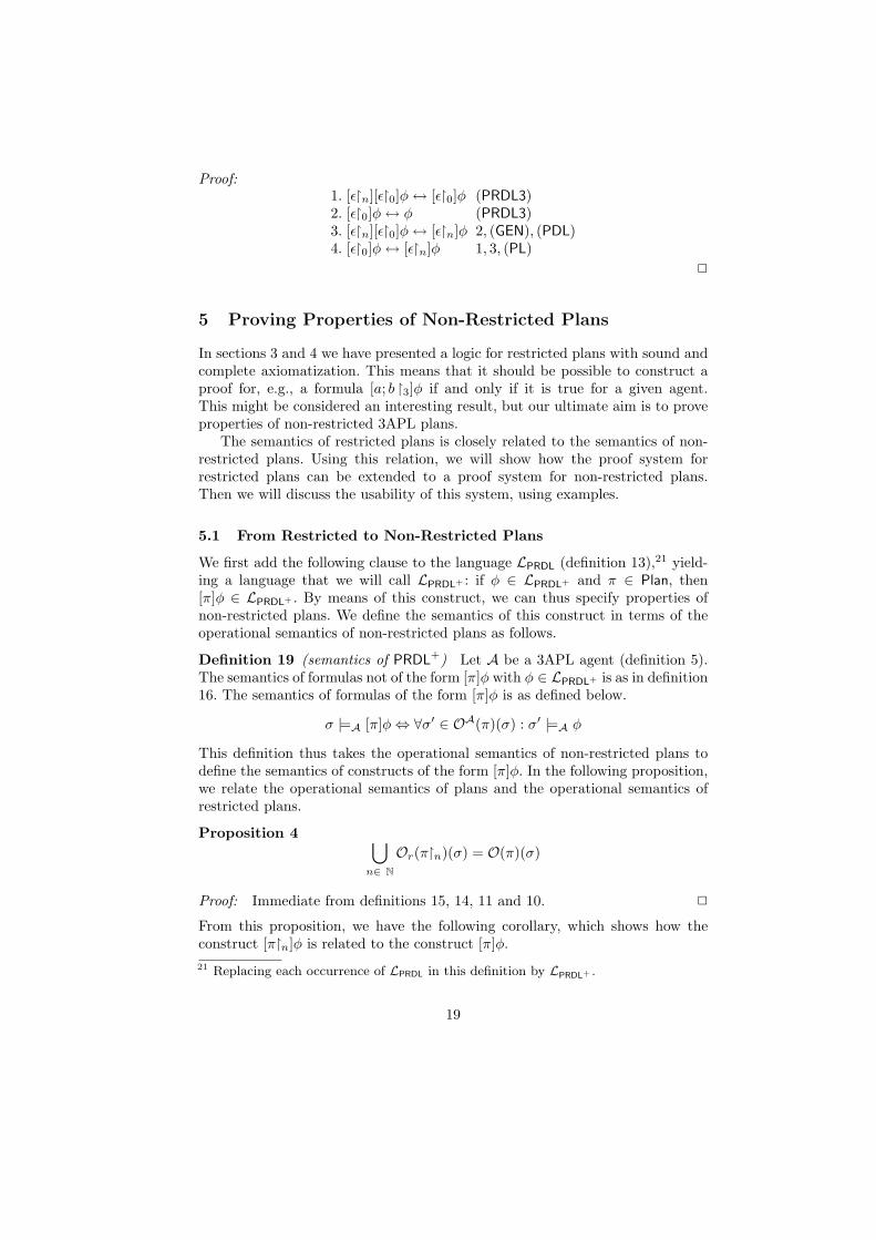
Proof:1. [εn][ε0]φ↔ [ε0]φ (PRDL3)2. [ε0]φ↔ φ (PRDL3)3. [εn][ε0]φ↔ [εn]φ 2, (GEN), (PDL)4. [ε0]φ↔ [εn]φ 1, 3, (PL)

2

5 Proving Properties of Non-Restricted Plans

In sections 3 and 4 we have presented a logic for restricted plans with sound andcomplete axiomatization. This means that it should be possible to construct aproof for, e.g., a formula [a; b 3]φ if and only if it is true for a given agent.This might be considered an interesting result, but our ultimate aim is to proveproperties of non-restricted 3APL plans.

The semantics of restricted plans is closely related to the semantics of non-restricted plans. Using this relation, we will show how the proof system forrestricted plans can be extended to a proof system for non-restricted plans.Then we will discuss the usability of this system, using examples.

5.1 From Restricted to Non-Restricted Plans

We first add the following clause to the language LPRDL (definition 13),21 yield-ing a language that we will call LPRDL+ : if φ ∈ LPRDL+ and π ∈ Plan, then[π]φ ∈ LPRDL+ . By means of this construct, we can thus specify properties ofnon-restricted plans. We define the semantics of this construct in terms of theoperational semantics of non-restricted plans as follows.

Definition 19 (semantics of PRDL+) Let A be a 3APL agent (definition 5).The semantics of formulas not of the form [π]φ with φ ∈ LPRDL+ is as in definition16. The semantics of formulas of the form [π]φ is as defined below.

σ |=A [π]φ⇔ ∀σ′ ∈ OA(π)(σ) : σ′ |=A φ

This definition thus takes the operational semantics of non-restricted plans todefine the semantics of constructs of the form [π]φ. In the following proposition,we relate the operational semantics of plans and the operational semantics ofrestricted plans.

Proposition 4 ⋃n∈ N

Or(πn)(σ) = O(π)(σ)

Proof: Immediate from definitions 15, 14, 11 and 10. 2

From this proposition, we have the following corollary, which shows how theconstruct [πn]φ is related to the construct [π]φ.21 Replacing each occurrence of LPRDL in this definition by LPRDL+ .

19

Corollary 1

∀n ∈ N : σ |=A [πn]φ⇔ ∀σ′ ∈ OA(π)(σ) : σ′ |=A φ⇔ σ |=A [π]φ

Proof: Immediate from proposition 4, definition 16 and definition 19. 2

From this corollary, we can conclude that we can prove a property of the form[π]φ by proving ∀n ∈ N : `Rule [πn]φ, using the system for restricted plans. Thisidea can be captured in a proof rule as follows.

Definition 20 (proof rule for non-restricted plans)

[πn]φ, n ∈ N[π]φ

This rule should be read as having an infinite number of premises, i.e., [π0]φ,[π1]φ, [π2]φ, . . . (see also [10]). Deriving a formula [π]φ using this infinitaryrule thus requires infinitely many premises to have been previously derived.

The rule is sound by corollary 1. The system ASRule for restricted plans(definition 17) taken together with the rule above, is a complete axiom systemfor PRDL+: if [π]φ is true then each of the premises of the rule is true (corollary1) and each of these premises can be proven by completeness of ASRule. Thenotion of a proof in this case is however non-standard, as a proof can be infinite.This completeness result is therefore theoretical, and putting the system to usein this way is obviously problematic.

One way to try to deal with this problem is the following. The idea isthat properties of the form ∀n ∈ N : `Rule [π n]φ can be proven by induc-tion on n, rather than proving [πn]φ for each n. If we can prove [π0]φ and∀n ∈ N : ([πn]φ `Rule [πn+1]φ), we can conclude the desired property. In thenext section we will illustrate how this could be done, using examples. The ex-amples however show that it is not obvious that this kind of induction can beapplied in all cases.

5.2 Examples

Example 2 Let A be an agent with one PR rule, i.e., Rule = a; b cand let T be such that [a0]φ, [b0]φ and [c0]φ. We now want to prove that∀n : [a; bn]φ. We have [a; b0]φ by using that this is equivalent to [a0][b0]φ byproposition 2. The latter formula can be derived by applying (GEN) to [b0]φ.We prove ∀n ∈ N : ([a; bn]φ `Rule [a; bn+1]φ) by taking an arbitrary n andproving that [a; bn]φ `Rule [a; bn+1]φ. Using (PRDL4) and (PRDL3), we havethe following equivalences.

[a; bn]φ↔ [a0][bn]φ ∧ [cn−1]φ↔ [a0][b0][εn]φ ∧ [c0][εn−1]φ↔ [a0][b0]φ ∧ [c0]φ

20

Similarly, we have the following equivalences for [a; bn+1]φ, yielding the desiredresult.

[a; bn+1]φ↔ [a0][bn+1]φ ∧ [cn]φ↔ [a0][b0][εn+1]φ ∧ [c0][εn]φ↔ [a0][b0]φ ∧ [c0]φ

4

Example 3 We will prove a property of a very simple 3APL agent usingaxiom (PRDL4) and induction on the number of PR rule applications. Our agenthas one PR rule: Rule = a a; a. Furthermore, assume that T is defined suchthat [a0]φ. We want to prove the following: ∀n ∈ N : [an]φ. In order to provethe desired result by induction on the number of PR rule applications, we thushave to prove [a0]φ and ∀n ∈ N : [an]φ `Rule [an+1]φ. [a0]φ was given. Letai denote a sequence of a’s of length i, with a0 = ε. The premiss of the secondconjunct can be rewritten using axiom (PRDL4) as follows.

[an]φ↔ [a0]φ ∧ [(a; a)n−1]φ↔ [a0]φ ∧ [a0][an−1]φ ∧ [(a; a; a)n−2]φ↔ [a0]φ ∧ [a0][an−1]φ ∧ [a0][(a; a)n−2]φ ∧ [(a; a; a; a)n−3]φ...↔ [a0]φ ∧ [a0][an−1]φ ∧ . . . ∧ [a0][(an)0]φ ∧ [(a; (an))0]φ

So, in order to prove [an+1]φ, we may assume - among other things - [an]φ,[(a; a) n−1]φ, [(a; a; a) n−2]φ, . . ., [(a; (an)) 0]φ (last conjunct of each line).Equivalently, we may thus assume the following.22∧

i

[(a; (ai))n−i]φ for 0 ≤ i ≤ n (5.1)

The consequent, i.e., [an+1]φ, can be rewritten using axiom (PRDL4) as below.

[an+1]φ↔ [a0]φ ∧ [(a; a)n]φ↔ [a0]φ ∧ [a0][an]φ ∧ [(a; a; a)n−1]φ↔ [a0]φ ∧ [a0][an]φ ∧ [a0][(a; a)n−1]φ ∧ [(a; a; a; a)n−2]φ...↔ [a0]φ ∧ [a0][an]φ ∧ . . . ∧ [a0][(a; (an))0]φ ∧ [(a; a; (an))0]φ

(5.2)As [an+1]φ is equivalent to all of the lines on the righthandside of (5.2), we mayprove any of these lines, in order to prove the desired result. As it turns out, itis easiest to prove the last line. The reason is that in this case, the last conjuncthas a restriction parameter of 0. We can thus use proposition 2 for sequential

22 Note that [a 0][(a0) n]φ ↔ [a 0][ε n]φ and [a 0][ε n]φ ↔ [a 0]φ, using axiom(PRDL3).

21

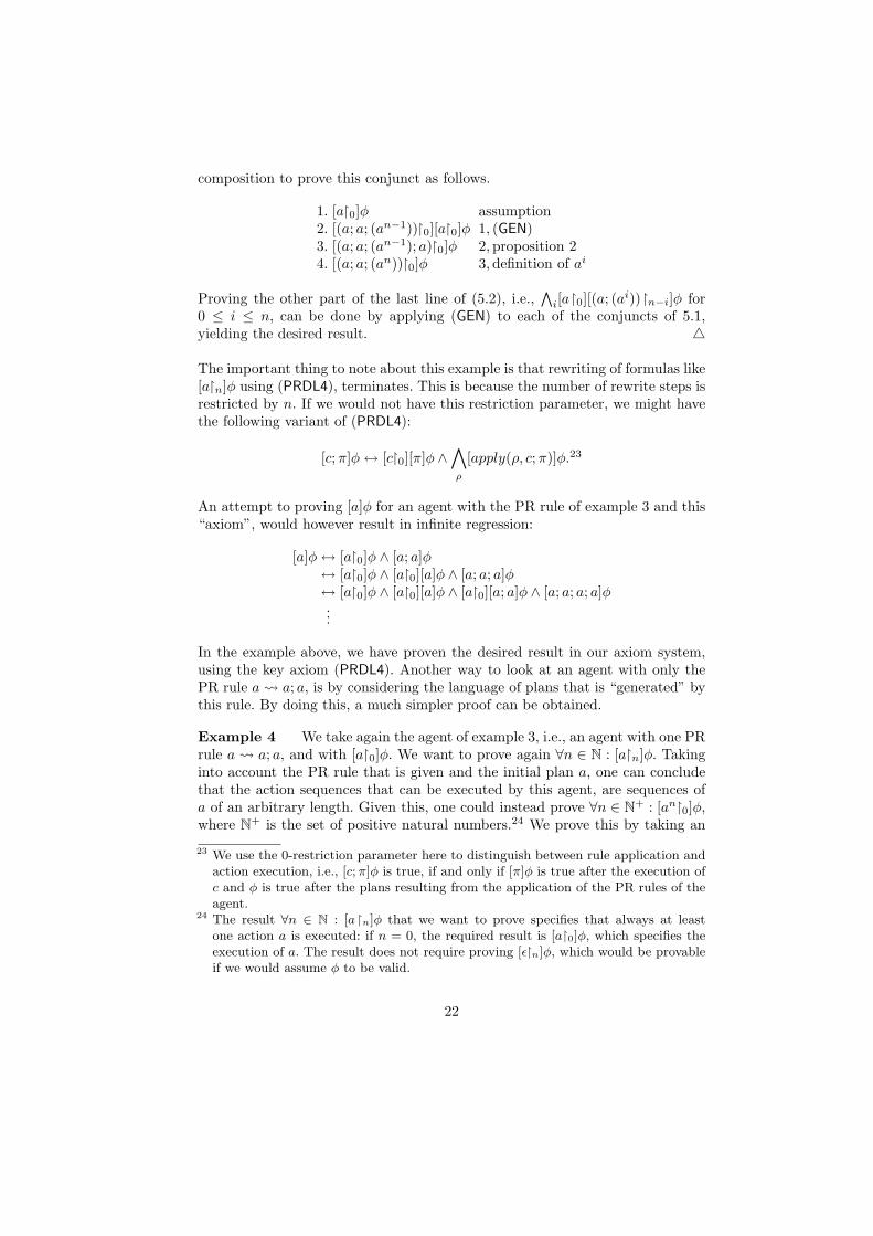
composition to prove this conjunct as follows.

1. [a0]φ assumption2. [(a; a; (an−1))0][a0]φ 1, (GEN)3. [(a; a; (an−1); a)0]φ 2,proposition 24. [(a; a; (an))0]φ 3,definition of ai

Proving the other part of the last line of (5.2), i.e.,∧

i[a0][(a; (ai))n−i]φ for

0 ≤ i ≤ n, can be done by applying (GEN) to each of the conjuncts of 5.1,yielding the desired result. 4

The important thing to note about this example is that rewriting of formulas like[an]φ using (PRDL4), terminates. This is because the number of rewrite steps isrestricted by n. If we would not have this restriction parameter, we might havethe following variant of (PRDL4):

[c;π]φ↔ [c0][π]φ ∧∧ρ

[apply(ρ, c;π)]φ.23

An attempt to proving [a]φ for an agent with the PR rule of example 3 and this“axiom”, would however result in infinite regression:

[a]φ↔ [a0]φ ∧ [a; a]φ↔ [a0]φ ∧ [a0][a]φ ∧ [a; a; a]φ↔ [a0]φ ∧ [a0][a]φ ∧ [a0][a; a]φ ∧ [a; a; a; a]φ...

In the example above, we have proven the desired result in our axiom system,using the key axiom (PRDL4). Another way to look at an agent with only thePR rule a a; a, is by considering the language of plans that is “generated” bythis rule. By doing this, a much simpler proof can be obtained.

Example 4 We take again the agent of example 3, i.e., an agent with one PRrule a a; a, and with [a0]φ. We want to prove again ∀n ∈ N : [an]φ. Takinginto account the PR rule that is given and the initial plan a, one can concludethat the action sequences that can be executed by this agent, are sequences ofa of an arbitrary length. Given this, one could instead prove ∀n ∈ N+ : [an0]φ,where N+ is the set of positive natural numbers.24 We prove this by taking an

23 We use the 0-restriction parameter here to distinguish between rule application andaction execution, i.e., [c; π]φ is true, if and only if [π]φ is true after the execution ofc and φ is true after the plans resulting from the application of the PR rules of theagent.

24 The result ∀n ∈ N : [a n]φ that we want to prove specifies that always at leastone action a is executed: if n = 0, the required result is [a0]φ, which specifies theexecution of a. The result does not require proving [εn]φ, which would be provableif we would assume φ to be valid.

22

arbitrary n and proving [an0]φ for this n.

1. [a0]φ assumption2. [a0][a0]φ 1, GEN3. [a; a0]φ 2, proposition 2

...[an0]φ

4

Obviously, this proof is much shorter than the proof of example 3. It is howeverobtained through meta-reasoning about the PR rules of the agent. In the desiredresult ∀n ∈ N+ : [an 0]φ, the restriction parameter is 0. The application ofPR rules has thus in effect been eliminated from the expression in the objectlanguage.

Meta-reasoning could be done in this simple case: the PR rule actually gener-ates the language of plans that can be represented by the simple regular expres-sion a∗. PR rules in general however do not only generate languages that can berepresented by regular expressions. In particular, rules of the form p π, wherep is an abstract plan, can be compared with parameterless recursive procedures(see also section 6), which can in turn be linked to context-free programs [10,Chapter 9]. Furthermore, PR rules can have the form πh πb, where the head isan arbitrary plan. It is thus not obvious that a meta-argument about the plansgenerated by the agent can be constructed in the general case. Investigationsalong these lines are however not within the scope of this paper and remain forfuture research.

In the next example, we will use proposition 5 below, in the proof of whichwe use the following lemma.

Lemma 2 Let Rule ⊆ R be a finite set of PR rules. The following is thenderivable in the axiom system ASRule.

`Rule [πn]φ→ [π0]φ

Proof: Let ci ∈ (BasicAction ∪ AbstractPlan) for i ≥ 1 and let π = c1; . . . ; cm,with m ≥ 1. Through repeated application of axiom (PRDL4), from left to right,then using (PRDL3) to get rid of [εn] and then using proposition 2 for sequentialcomposition with a 0 restriction parameter, we derive the desired result.

[πn]φ↔ [c1; . . . ; cmn]φ→ [c10][c2; . . . ; cmn]φ→ . . .→ [c10][c20] . . . [cm0][εn]φ→ [c10][c20] . . . [cm0]φ→ [c1; c20][c30] . . . [cm0]φ→ . . .→ [c1; . . . ; cm0]φ→ [π0]φ

23

2

In the following proposition, we will use some notation that we will first explain.The notation (PRDL4)i([π n]φ), with 0 ≤ i ≤ n, denotes the formula thatresults from rewriting [π n]φ using (PRDL4) from left to right, such that allrestriction parameters are either 0 or i. Formulas of the form [εm]φ are replacedby φ, using axiom (PRDL3). In this process, (PRDL4) may only be applied to aformula [πm]φ if m > i.

Take, e.g., the agent of example 3 with a a; a as the only PR rule. Theformula (PRDL4)3([a5]φ) then for example denotes the formula [a0]φ∧ [a0][a0]φ ∧ [a0][a; a3]φ ∧ [a; a; a3]φ, which can be obtained by rewriting the formula[a5]φ as below.

[a5]φ↔ [a0][ε5]φ ∧ [a; a4]φ↔ [a0]φ ∧ [a0][a4]φ ∧ [a; a; a3]φ↔ [a0]φ ∧ [a0][a0][ε4]φ ∧ [a0][a; a3]φ ∧ [a; a; a3]φ↔ [a0]φ ∧ [a0][a0]φ ∧ [a0][a; a3]φ ∧ [a; a; a3]φ

The idea is thus, that formulas of the form [πm]φ are rewritten until formulasare obtained with i as the restriction parameter. A formula [πi]φ may not berewritten.

Any formula [πn]φ can be rewritten into a formula (PRDL4)i([πn]φ) with0 ≤ i ≤ n. An application of (PRDL4) to a formula [πm]φ yields two conjuncts(the second of which is again a conjunction). The first conjunct is smaller inplan size than [πm]φ.25 Each conjunct of the second conjunct is smaller than[π m]φ with respect to the restriction parameter. With each rewrite step, wethus have a decrease either in plan size or in size of the restriction parameter ofeach resulting conjunct. This can thus continue for each conjunct until either theplan size (minus the plan size of φ) is 0 or the non-zero restriction parametersare equal to i.

Another notation that we will use is to0(φ), denoting the formula that resultsfrom replacing all restriction parameters in φ by 0.

Proposition 5 (restriction parameter) Let Rule ⊆ R be a finite set of PRrules. The following is then derivable in the axiom system ASRule.

`Rule [πn]φ→ [πi]φ with − 1 ≤ i ≤ n

Proof: If i = −1, the desired result follows immediately by axiom (PRDL1). Wewill now prove the result for i ≥ 0.

1. [πn]φ↔ (PRDL4)n−i([πn]φ) (PRDL4)2. [πi]φ↔ (PRDL4)0([πi]φ) (PRDL4)3. (PRDL4)n−i([πn]φ) → to0((PRDL4)n−i([πn]φ)) lemma 24. to0((PRDL4)n−i([πn]φ)) ↔ (PRDL4)0([πi]φ) syntactic equality5. (PRDL4)n−i([πn]φ) → (PRDL4)0([πi]φ) 3, 46. [πn]φ→ [πi]φ 1, 2, 5

25 The second element of size(F ), where F denotes the first conjunct, is smaller thanthe second element of size([πm]φ.

24

Step 4 is justified, because both (PRDL4)n−i([πn]φ) and (PRDL4)0([πi]φ) resultfrom the same number of applications of (PRDL4) to [πn]φ and [πi]φ respec-tively. The latter two formulas are syntactically equal, except for the restrictionparameter. The formulas (PRDL4)n−i([π n]φ) and (PRDL4)0([π i]φ) are thusalso syntactically equal,26 except for the restriction parameters, which are n− ior 0 in the first case and 0 in the latter. Setting the restriction parameters ofthe first formula to 0, will thus give us equivalent formulas. 2

Example 5 We now consider an agent with two PR rules: Rule = a a; a, a; a; a b and we assume that [a 0]φ and [b 0]φ. We want to prove∀n ∈ N : [a n]φ. Along similar lines of reasoning as in example 3, i.e., byusing axiom (PRDL4) to rewrite [an]φ, we can conclude that we may again useassumption (5.1) from example 3. We have to prove the following, taking the“last line” of the rewriting of [an+1]φ by (PRDL4).∧

i

[a0][(a; (ai))n−i]φ for 0 ≤ i ≤ n (5.3)∧i

[(b; (ai−2))n−i]φ for 2 ≤ i ≤ n (5.4)

[(a; a; (an))0]φ (5.5)

The formulas (5.3) and (5.5) were proven in the example above, using assumption(5.1). We will prove (5.4) by proving

∧i[(a

i−2)n−i]φ and using (GEN) to derivethe desired formula.

In the proof below, let 3 ≤ i ≤ n and let 0 ≤ r ≤ n in the first line and0 ≤ r ≤ n− 3 in the second line.

1.∧

r[(a; (ar))n−r]φ assumption (5.1)

2.∧

r[(a; (ar))n−r−3]φ 1,proposition 5

3.∧

i[(a; (ai−3))n−i]φ where r = i− 3

4.∧

i[(ai−2)n−i]φ definition of ai

5.∧

i[b0][(ai−2)n−i]φ 4, (GEN)

6.∧

i[b0][(ai−2)n−i]φ↔

∧i[(b; (a

i−2))n−i]φ (PRDL4)7.

∧i[(b; (a

i−2))n−i]φ 5, 6, (MP)

The above proves [(b; (ai−2))n−i]φ for 3 ≤ i ≤ n. If i = 2, we need to prove[bn−2]φ. According to axiom (PRDL4), this is equivalent to proving [b0]φ.27

This was given, so we are done. 4

In section 5.1, we have presented an infinitary axiom system to prove propertiesof non-restricted 3APL plans. As an infinitary axiom system is difficult to use,we have suggested to use induction on the number of PR rule applications, i.e.,on the restriction parameter, in an expression. Some examples have been worked26 That is, modulo swapping of conjuncts.27 By (PRDL4) we have [bn−2]φ ↔ [b0][εn−2]φ and by (PRDL3): [b0][εn−2]φ ↔ [b0

]φ.

25

out to illustrate this approach. As the examples show, it is doable (at least forthe example cases) to use induction on the number of PR rule applications. Itis however a fairly complicated undertaking. Future research will have to showwhether this type of reasoning is amenable to some kind of automation, andwhat the limits of the approach are.

6 PR Rules versus Procedures

As stated in the introduction, the operational semantics of (parameterless) pro-cedures is similar to that of PR rules. The operational semantics of a procedurep ⇐ S where p is the procedure name and the statement S is the body of theprocedure, can be defined by a transition 〈p;S′, σ〉 → 〈S;S′, σ〉, where S′ is astatement. If we compare this semantics to the semantics of PR rules of defi-nition 7, we can see that both are so-called body-replacement semantics: if thehead of a PR rule or the name of a procedure occur at the head of a statementthat is to be executed, the head or the procedure name are replaced by the bodyof the rule or the procedure respectively.

Because of this similarity, one might think that techniques used for reasoningabout procedures can be used to reason about PR rules. This however turns outnot to be the case, due to the non-compositional semantics of the sequentialcomposition operator in 3APL (see introduction of section 3). In this section,we will elaborate on this issue by studying inference rules of Hoare logic forreasoning about procedures (see for example [6,1] for a detailed explanation ofHoare logic). We will also show that reasoning by induction on the number ofPR rule applications and reasoning about procedures using Hoare logic inferencerules, although very different at first sight, actually do have similarities.

6.1 Reasoning about Procedures

Hoare logic is used for reasoning about programs. Inference rules are definedto derive so-called Hoare triples. A Hoare triple is of the form φ1 S φ2and intuitively means that if φ1 holds, φ2 will always hold after the executionof the statement S.28 To reason about non-recursive procedures, the followinginference rule can be defined for a procedure p ⇐ S (for simplicity, we assumewe only have one procedure) with procedure name p and body S.

φ1 S φ2φ1 p φ2

The rule states that if we can prove that φ2 holds after the execution of the bodyS of the procedure (assuming φ1 holds before execution), we can infer that φ2

holds after the procedure call p.

28 The Hoare triple φ1 S φ2 can be characterized in dynamic logic by the formulaφ1 → [S]φ2.

26

If the procedure p⇐ S is recursive, that is, if p is called in S, the rule abovewill still be sound, but a system with only this rule for reasoning about procedurecalls will not be complete (see also [1]). An attempt at proving φ1 p φ2 resultsin an infinite regression. The following rule [1], which is a variant of so-calledScott’s induction rule (see for example [6]), is meant to overcome this difficulty.

Definition 21 (Scott’s induction rule)

φ1 p φ2 ` φ1 S φ2φ1 p φ2

The rule states that if we can prove φ1 S φ2 from the assumption thatφ1 p φ2, we can infer φ1 p φ2. Using this rule for reasoning aboutprocedure calls, a complete proof system can be obtained [1].29

In a proof of a property of a procedural program, the rule above is (often)used in combination with the following rule for sequential composition.

Definition 22 (rule for sequential composition)

φ1 S φ2 φ2 S′ φ3φ1 S;S′ φ3

Consider for example a procedure p ⇐ p and suppose we want to proveφ1 p;S φ3 (p is non-terminating, so we should be able to prove this forany φ1 and φ3). We then have to prove φ1 p φ2 and φ2 S φ3 for someφ2. If we take φ2 = 0, i.e., falsum, the second conjunct follows immediately. Inproving φ1 p 0, which we will refer to as H, we use Scott’s induction ruleand we thus have to prove H from the assumption that H. This is immediate,concluding the proof.

The point of this example is the following. Using Scott’s induction rule, wecan prove properties of a procedure call p. If we want to prove a property of astatement involving the sequential composition of this procedure call and someother statement S, we can use properties proven of the procedure call (obtainedusing Scott’s induction rule) and compose it with properties proven of S bymeans of the rule for sequential composition. In particular, this technique canbe applied to for example a procedure p ⇐ p;S, where an assumption aboutp can be used to prove properties of p;S. Scott’s induction rule for provingproperties of procedure calls is thus most useful if used in combination with therule for sequential composition.

Scott’s induction rule for PR rules A question one might ask, is whether avariant of Scott’s induction rule can be used to reason about PR rules. Assuming

29 Note that this is a proof rule for deriving partial correctness specifications, a Hoaretriple φ1 p φ2 meaning that if p terminates, φ2 will hold after execution of p(provided that p is executed in a state in which φ1 holds). If p does not terminate,anything is derivable for p. The rule cannot be used to prove termination of p.

27

one PR rule πh πb, the following rule could be formulated.

φ1 πh φ2 ` φ1 πb φ2φ1 πh φ2

Assume for the moment that it is possible to use this rule to prove φ1 πh φ2for some PR rule πh πb and properties φ1 and φ2. The question now is,whether the fact that we can prove φ1 πh φ2, will do us any good if we wantto prove properties of more complex plans such as πh;π.

Proving properties of πh;π based on properties proven of πh, would have to bedone using the rule for sequential composition. This rule is however not soundin the context of PR rules. In general, it is not the case that O(π1;π2)(σ) ⊆O(π2)(O(π1)(σ)) (see also the introduction of section 3). Let Σ1 = O(π1)(σ)and Σ2 = O(π2)(Σ1). If φ2 holds in all states in Σ1 (if φ1 holds in σ), thenφ3 will hold in all states in Σ2 by assumption. Let Σ3 = O(π1;π2)(σ) and letσ′ ∈ Σ3, but σ′ 6∈ Σ2. Then we may not conclude that φ3 will hold in σ′ andtherefore the rule is not sound.

The fact that we can prove φ1 πh φ2, will thus not help if we want toprove properties of a plan like πh;π, because we do not have a rule for sequen-tial composition. In particular, the assumption φ1 πh φ2 will not help toprove φ1 πb φ2, even if πb = πh;π. It is thus not clear whether it shouldbe possible in the general case to prove φ1 πb φ2 from the assumptionφ1 πh φ2. Moreover, the rule above is not sound for agents with more thanone PR rule. It is then in general not the case that O(πb)(σ) = O(πh)(σ), ratherO(πb)(σ) ⊆ O(πh)(σ). Therefore, we may not conclude φ1 πh φ2 from aproof of φ1 πb φ2.

6.2 Induction

In section 6.1 we argued that, although the operational semantics of PR rules andprocedure calls are very similar, we cannot use Scott’s induction rule, which isused for reasoning about procedure calls, to reason about PR rules. Our solutionto the issue of reasoning about PR rules as presented in this paper, is to doinduction on the number of PR rule applications. In this section, we will elaborateon why Scott’s induction rule is called an induction rule and by doing this, wewill see that induction on the number of PR rule applications and induction asused in Scott’s induction rule, have strong similarities.

At first sight, it does not look like using Scott’s induction rule involves doinginduction, because we do not see formulas parameterized with natural numbersn and n+ 1. To see why the rule actually is an induction rule, we first rephrasethe rule of definition 21 and adopt notation used by De Bakker [6]. Ω is used todenote a non-terminating statement (similar to the fail statement mentioned inthe proof of theorem 2). The first element of a tuple 〈. . . | . . .〉 is used to indicatethe procedures, in the presence of which the formula of the second element shouldhold.

φ1 Ω φ2 〈 | φ1 p φ2 ` φ1 S φ2〉〈p⇐ S | φ1 p φ2〉

(6.1)

28

The rule above is an instantiation of a more general version of this rule formultiple procedures [6]. The first antecedent is derived from this general rule, butcould be omitted in this form: Ω is a non-terminating statement and thereforethe triple φ1 Ω φ2 is valid for any φ1, φ2. We will however not eliminate itfor the purpose of comparing this rule with reasoning about PR rules.

Now, consider a procedure p ⇐ S and let Sn be defined as follows: S0 = Ωand Sn+1 = S[Sn/p], where S[Sn/p] means that every occurrence of p in Sis replaced by Sn. If for example S = p;S′, then S1 = S0;S′ = Ω;S′, S2 =S1;S′ = (Ω;S′);S′, etc.

Using this substitution construction, we can define the meaning M of aprocedure p ⇐ S in the following way (see Apt [1]): M(p) =

⋃∞n=0M(Sn).

From this, we can conclude that 〈p⇐ S | φ1 p φ2〉 is true iff ∀n : 〈p⇐ Sn |φ1 p φ2〉 is true [1]. Therefore, the induction rule above is equivalent withthe following rule.

φ1 Ω φ2 〈 | φ1 p φ2 ` φ1 S φ2〉∀n : 〈p⇐ Sn | φ1 p φ2〉

(6.2)

The meaning of a procedure call p of a procedure p ⇐ S is equivalent with themeaning of S. More in general, the meaning of a statement S′ in which a callto procedure p ⇐ S occurs, is equivalent with the meaning of the statementS′[S/p], i.e., the statement S′ in which all occurrences of p are replaced with S(see [6]). Therefore, we may replace p with Sn in rule (6.2) and we may replaceoccurrences of p in S with Sn. We have by definition that S[Sn/p] = Sn+1,yielding the following equivalent rule30.

φ1 Ω φ2 ∀n : (φ1 Sn φ2 ` φ1 Sn+1 φ2)∀n : φ1 Sn φ2

(6.3)

This rule, which is equivalent with Scott’s induction rule, demonstrates clearlywhy Scott’s induction rule is called an induction rule. The idea of proving prop-erties of a 3APL agent of the form ∀n : `Rule [πn]φ by induction on n, is thatwe prove [π0]φ and ∀n : ([πn]φ `Rule [πn+1]φ). The similarity between the twoapproaches is thus that induction on respectively the number of procedure callsand PR rule applications is done (implicitly or explicitly).

The important difference however is that the statement S in rule (6.3) cor-responds with the body of a procedure p in the equivalent rule (6.1). The planπ on the other hand does not correspond with the body of a PR rule, but ratherrefers to the initial plan of the agent. Related to this is the fact that rule (6.3) orthe equivalent rule (6.1) can be used in combination with the rule for sequentialcomposition, as explained in section 6.1. In the case of using induction to reasonabout 3APL plans, this is impossible.

Concluding, the general idea of doing induction on the number of PR ruleapplications is less obscure than one might have thought at first sight, because

30 We omit the procedure declaration p ⇐ S, because there are no occurrences of p ineither Sn or Sn+1 by definition.

29

of the similarity with the standard Scott’s induction rule. The way in whichinduction can be used to prove properties of plans or programs, however dif-fers between the two approaches due to the non-compositional semantics of thesequential composition operator in plans, as a result of the presence of PR rules.

7 Conclusion

In this paper, we presented a dynamic logic for reasoning about 3APL agents,tailored to handle the plan revision aspect of the language. As we argued, 3APLplans cannot be analyzed by structural induction, which means that standardpropositional dynamic logic cannot be used to reason about 3APL plans. Instead,we proposed a logic of restricted plans with sound and complete axiomatization.We also showed that this logic can be extended to a logic for non-restrictedplans. This however results in an infinitary axiom system. We suggested thata possible way of dealing with the infinitary nature of the axiom system, isreasoning by induction on the restriction parameter. We showed some examplesof how this could be done. Finally, we discussed the relation between PR rulesand procedures. In particular, we argued that there is a similarity between theuse of Scott’s induction rule for reasoning about procedures, and the use ofinduction on the number of PR rules applications for reasoning about PR rules.

Concluding, being able to do structural induction is usually considered an es-sential property of programs in order to reason about them. As 3APL plans lackthis property, it is not at all obvious that it should be possible to reason aboutthem, especially using a clean logic with sound and complete axiomatization.The fact that we succeeded in providing such a logic, thus at least demonstratesthis possibility. The resulting infinitary axiom system is nevertheless more of the-oretical than practical importance. Future research will have to show whetherreasoning by doing induction on the number of PR rule applications is amenableto some kind of automation, working towards an extension of these results to amore practical setting. Another important line for future research is the investi-gation of the relation between term rewriting systems and PR rules, and betweenPR rules and formal language theory. We hope that those investigations will leadto the definition of interesting subclasses of PR rules that can be analyzed bystructural induction.

References

1. K. R. Apt. Ten years of Hoare’s logic: A survey - part I. ACM Transactions ofProgramming Languages and Systems, 3(4):431–483, 1981.

2. R. H. Bordini, M. Fisher, C. Pardavila, and M. Wooldridge. Model checkingAgentSpeak. In Proceedings of the second international joint conference on au-tonomous agents and multiagent systems (AAMAS’03), pages 409–416, Melbourne,2003.

3. M. E. Bratman. Intention, plans, and practical reason. Harvard University Press,Massachusetts, 1987.

30

4. P. R. Cohen and H. J. Levesque. Intention is choice with commitment. ArtificialIntelligence, 42:213–261, 1990.

5. M. Dastani, M. B. van Riemsdijk, F. Dignum, and J.-J. Ch. Meyer. A programminglanguage for cognitive agents: goal directed 3APL. In Programming multiagentsystems, first international workshop (ProMAS’03), volume 3067 of LNAI, pages111–130. Springer, Berlin, 2004.

6. J. de Bakker. Mathematical Theory of Program Correctness. Series in ComputerScience. Prentice-Hall International, London, 1980.

7. R. Evertsz, M. Fletcher, R. Jones, J. Jarvis, J. Brusey, and S. Dance. Implementingindustrial multi-agent systems using JACK. In Proceedings of the first interna-tional workshop on programming multiagent systems (ProMAS’03), volume 3067of LNAI, pages 18–49. Springer, Berlin, 2004.

8. G. d. Giacomo, Y. Lesperance, and H. Levesque. ConGolog, a Concurrent Pro-gramming Language Based on the Situation Calculus. Artificial Intelligence, 121(1-2):109–169, 2000.

9. D. Harel. First-Order Dynamic Logic. Lectures Notes in Computer Science 68.Springer, Berlin, 1979.

10. D. Harel, D. Kozen, and J. Tiuryn. Dynamic Logic. The MIT Press, Cambridge,Massachusetts and London, England, 2000.

11. M. Hinchey, J. Rash, W. Truszkowski, C. Rouff, and D. Gordon-Spears, editors.Formal Approaches to Agent-Based Systems (Proceedings of FAABS’02), volume2699 of LNAI, Berlin, 2003. Springer.

12. K. V. Hindriks, F. S. de Boer, W. van der Hoek, and J.-J. Ch. Meyer. Agentprogramming in 3APL. Int. J. of Autonomous Agents and Multi-Agent Systems,2(4):357–401, 1999.

13. K. V. Hindriks, F. S. de Boer, W. van der Hoek, and J.-J. Ch. Meyer. A pro-gramming logic for part of the agent language 3APL. In Proceedings of the FirstGoddard Workshop on Formal Approaches to Agent-Based Systems (FAABS’00),2000.

14. A. S. Rao. AgentSpeak(L): BDI agents speak out in a logical computable language.In W. van der Velde and J. Perram, editors, Agents Breaking Away (LNAI 1038),pages 42–55. Springer-Verlag, 1996.

15. A. S. Rao and M. P. Georgeff. Modeling rational agents within a BDI-architecture.In J. Allen, R. Fikes, and E. Sandewall, editors, Proceedings of the Second Inter-national Conference on Principles of Knowledge Representation and Reasoning(KR’91), pages 473–484. Morgan Kaufmann, 1991.

16. J. Rash, C. Rouff, W. Truszkowski, D. Gordon, and M. Hinchey, editors. FormalApproaches to Agent-Based Systems (Proceedings of FAABS’01), volume 1871 ofLNAI, Berlin, 2001. Springer.

17. Y. Shoham. Agent-oriented programming. Artificial Intelligence, 60:51–92, 1993.18. W. van der Hoek, B. van Linder, and J.-J. Ch. Meyer. An integrated modal

approach to rational agents. In M. Wooldridge and A. S. Rao, editors, Foundationsof Rational Agency, Applied Logic Series 14, pages 133–168. Kluwer, Dordrecht,1998.

19. P. van Emde Boas. The connection between modal logic and algorithmic logics.In Mathematical foundations of computer science 1978, volume 64 of LNCS, pages1–15. Springer, Berlin, 1978.

20. M. B. van Riemsdijk, F. S. de Boer, and J.-J. Ch. Meyer. Dynamic logic for planrevision in intelligent agents. In J. A. Leite and P. Torroni, editors, Proceedingsof the fifth international workshop on computational logic in multi-agent systems(CLIMA’04), pages 196–211, 2004. To appear in LNAI 3487.

31

21. M. B. van Riemsdijk, J.-J. Ch. Meyer, and F. S. de Boer. Semantics of planrevision in intelligent agents. In C. Rattray, S. Maharaj, and C. Shankland, editors,Proceedings of the 10th International Conference on Algebraic Methodology AndSoftware Technology (AMAST04), volume 3116 of LNCS, pages 426–442. Springer-Verlag, 2004. Extended version is to appear in special issue of TCS.

22. M. B. van Riemsdijk, W. van der Hoek, and J.-J. Ch. Meyer. Agent program-ming in Dribble: from beliefs to goals using plans. In Proceedings of the secondinternational joint conference on autonomous agents and multiagent systems (AA-MAS’03), pages 393–400, Melbourne, 2003.

23. M. Wooldridge. Agent-based software engineering. IEEE Proceedings SoftwareEngineering, 144(1):26–37, 1997.

32