dynamic law of physical motion and

DYNAMIC LAW OF PHYSICAL MOTION ANDPOTENTIAL-DESCENDING PRINCIPLE

TIAN MA AND SHOUHONG WANG

Abstract. The main objectives of this paper are five-fold. Thefirst is to introduce a general dynamic law for all physical mo-tion systems, based on a new variational principle with constraint-infinitesimals. The second is to postulate the potential-descendingprinciple (PDP). We show that PDP is a more fundamental prin-ciple than the first and second laws in thermodynamics, and givesrise to dynamical equations for non-equilibrium systems. Thethird is to demonstrate that the PDP is the first principle todescribe irreversibility of all thermodynamic systems, with ther-modynamic potential as the basic physical quantity, rather thanentropy. The fourth objective is to examine the problems facedby the Boltzmann equation. We show that the Boltzmann is nota physical law, is created as a mathematical model to obey theentropy-increasing principle (for dilute gases), and consequently isunable to faithfully describe Nature. The fifth objective is to provean orthogonal-decomposition theorem and a theorem on variationwith constraint-infinitesimals, providing the needed mathematicalfoundations of the dynamical law of physical motion.

Contents

1. Introduction 22. Dynamic Law of Physical Motion 82.1. General guiding principles 82.2. Principle of symmetry-breaking 82.3. Dynamic Law of Physical Motion 93. Potential-Descending Principle in Statistical Physics 123.1. Thermodynamic potentials 12

Date: July 5, 2017.Key words and phrases. dynamical law of physical motion, potential-descending

principle, statistical physics, thermodynamics, entropy, irreversible processes Boltz-mann equation, orthogonal-decomposition theorem, variation with constraint-infinitesimals.

The work was supported in part by the US National Science Foundation(NSF), the Office of Naval Research (ONR) and by the Chinese National ScienceFoundation.

1

2 MA AND WANG

3.2. Potential-Descending Principle in Statistical Physics 133.3. Minimum potential principle 143.4. PDP-based mathematical models 153.5. Diffusion and heat conductivity equation 164. Irreversibility in Thermodynamic Systems 165. Problems in Boltzmann Equation 185.1. Boltzmann equation 185.2. Problems in Boltzmann equation 205.3. Conclusions 226. Mathematical Foundations of Dynamic Law 226.1. General orthogonal Decomposition Theorem 226.2. Variations with constrained-infinitesimals 247. Dynamics of Other Physical Motion Systems 267.1. Newtonian laws 267.2. Fluid Dynamics 267.3. Hamiltonian dynamics 287.4. Lagrangian Dynamics 28References 29

1. Introduction

The heart of physics is to seek experimentally verifiable, fundamentallaws and principles of Nature. In this process, physical concepts andtheories are transformed into mathematical models and the predictionsderived from these models can be verified experimentally and conformto reality. In their mathematical form, the physical laws are often canbe expressed as mathematical equations:

physical laws = mathematical equations.

Among most important physical laws are 1) the laws for fundamentalinteractions —- gravity, electromagnetism, weak and strong —- and 2)the laws for motion dynamics. Modern theory of fundamental interac-tions is based on the field theoretical point of view; see among manyothers [4] and their references therein.

The focus of this paper is on dynamical laws of physical motion sys-tems. According to their scales, the physical motion systems include1) classical mechanical systems, describing planetary scale motion, 2)quantum systems for particles in the micro level, 3) fluid mechanics sys-tems, macroscopic description of fluid motion, 4) astrophysical systemsfor astronomical objects, and 5) statistical systems, relating micro-scopic properties of individual particles to the macroscopic properties.

MOTION LAW & POTENTIAL-DESCENDING PRINCIPLE 3

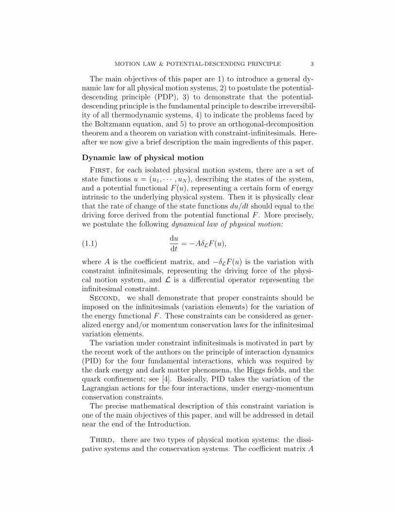
The main objectives of this paper are 1) to introduce a general dy-namic law for all physical motion systems, 2) to postulate the potential-descending principle (PDP), 3) to demonstrate that the potential-descending principle is the fundamental principle to describe irreversibil-ity of all thermodynamic systems, 4) to indicate the problems faced bythe Boltzmann equation, and 5) to prove an orthogonal-decompositiontheorem and a theorem on variation with constraint-infinitesimals. Here-after we now give a brief description the main ingredients of this paper.

Dynamic law of physical motion

First, for each isolated physical motion system, there are a set ofstate functions u = (u1, · · · , uN), describing the states of the system,and a potential functional F (u), representing a certain form of energyintrinsic to the underlying physical system. Then it is physically clearthat the rate of change of the state functions du/dt should equal to thedriving force derived from the potential functional F . More precisely,we postulate the following dynamical law of physical motion:

(1.1)du

dt= −AδLF (u),

where A is the coefficient matrix, and −δLF (u) is the variation withconstraint infinitesimals, representing the driving force of the physi-cal motion system, and L is a differential operator representing theinfinitesimal constraint.

Second, we shall demonstrate that proper constraints should beimposed on the infinitesimals (variation elements) for the variation ofthe energy functional F . These constraints can be considered as gener-alized energy and/or momentum conservation laws for the infinitesimalvariation elements.

The variation under constraint infinitesimals is motivated in part bythe recent work of the authors on the principle of interaction dynamics(PID) for the four fundamental interactions, which was required bythe dark energy and dark matter phenomena, the Higgs fields, and thequark confinement; see [4]. Basically, PID takes the variation of theLagrangian actions for the four interactions, under energy-momentumconservation constraints.

The precise mathematical description of this constraint variation isone of the main objectives of this paper, and will be addressed in detailnear the end of the Introduction.

Third, there are two types of physical motion systems: the dissi-pative systems and the conservation systems. The coefficient matrix A

4 MA AND WANG

is symmetric and positive definite if and only if the system is a dissi-pative system, and A is anti-symmetry if and only if the system is aconservation system.

Fourth, symmetry plays a fundamental role in understanding Na-ture. In [4], we have demonstrated that for the four fundamental inter-actions, the Lagrangian actions are dictated by the general covariance(principle of general relativity), the gauge symmetry and the Lorentzsymmetry; the field equations are then derived using PID as mentionedearlier.

For isolated motion systems, all energy functionals F obey certainsymmetries such as SO(n) (n = 2, 3) symmetry. In searching for lawsof Nature, one inevitably encounters a system consisting of a number ofsubsystems, each of which enjoys its own symmetry principle with itsown symmetry group. To derive the basic law of the coupled system,we have demonstrated in [4] the principle of symmetry-breaking (PSB),which is of fundamental importance for deriving physical laws for bothfundamental interactions and motion dynamics:

Physical systems in different levels obey different laws,which are dictated by their corresponding symmetries.For a system coupling different levels of physical laws,part of these symmetries must be broken.

In view of this principle, for a system coupling different subsystems,the motion equations become

(1.2)du

dt= −AδLF (u) +B(u),

where B(u) represents the symmetry-breaking. As we shall see in Sec-tion 4, all physical motions systems coupling different subsystems aregoverned by the above dynamical law (1.2).

Fifth, the dynamical law given by (1.1) and (1.2) is essentiallyknown for motion system in classical mechanics, quantum mechanicsand astrophysics; see among others [1, 4]. Thanks to the variation withinfinitesimal constraints, the law of fluid motion is now in the form of(1.1) and (1.2). The potential-descending principle given below showsthat non-equilibrium thermodynamical systems are governed by thedynamical law (1.1) and (1.2), as well.

Potential-Descending PrincipleAfter a thorough examination of thermodynamics, we discover that

the Potential-Descending Principle (PDP), which we shall postulatebelow, is a more fundamental principle in statistical principle.


First, for a given thermodynamic system, the order parameters(state functions) u = (u1, · · · , uN), the control parameters λ, and thethermodynamic potential (or potential in short) F are well-definedquantities, fully describing the system. The potential is a functionalof the order parameters, and is used to represent the thermodynamicstate of the system. There are four commonly used thermodynamicpotentials: the internal energy, the Helmholtz free energy, the Gibbsfree energy, and the enthalpy.

We postulate now the potential-descending principle (PDP) as fol-lows; see Principle 3.1 a more complete statement of this principle: Fora non-equilibrium state u(t;u0) of a thermodynamic system with initialstate u(0, u0) = u0,

1) the potential F (u(t;u0);λ) is strictly decreasing astime evolves;

2) the order parameters u(t;u0), as time evolves to in-finity, tends to an equilibrium of the system, whichis a minimal point of the potential F .

Second, we show in Section 3.3 that PDP leads to both the firstand the second laws of thermodynamics. In the classical thermody-namics theory (e.g. [6]), the perception is that potential-decreasingproperty can be derived from the first and second laws. However, inthe derivations, there is a hidden assumption that at the equilibrium,there is a free-variable in each of the conjugate pairs. For example,in the internal energy system, the entropy S and the generalized dis-placement X are free variables. This assumption is mathematicallyequivalent to the potential-descending principle. In other words, thepotential-decreasing property cannot be derived if we treat the firstand second laws as the only fundamental principles of thermodynam-ics. We refer Section 3.3 for details. Therefore we reach the followingconclusion:

the potential-descending principle leads to both the firstand second laws of thermodynamics, and the potential-descending principle is a more fundamental principlethen the first and second laws.

Hereafter we shall also show that PDP provides the first principlefor describing irreversibility.

Third, PDP provides dynamic equations for a non-equilibrium ther-modynamic system, which take exactly the form given by (1.1) or (1.2);see also (3.9) and (3.10).

Irreversibility

6 MA AND WANG

We know that the motion of all statistical physical system (collectionof large number of particles) possesses irreversibility. Classical thermo-dynamics attributes this irreversibility to entropy-increasing principle.We show in this paper, however, that the Potential-Descending Princi-ple (PDP) is the first principle for irreversibility for all thermodynamicsystems. The main reasons are as follows.

First, PDP indeed offers a clear description of the irreversibility ofthermodynamical systems. Consider a non-equilibrium initial state u0

of the thermodynamic system with order parameters u, control param-eters λ and potential F , the PDP amounts to saying that the potentialis decreasing:

d

dtF (u(t;u0);λ) < 0 ∀t > 0.

This shows that the state of the system u(t;u0) will never return to itsinitial state u0 in the future time. This is exactly the irreversibility.

Second, entropy S is a state function, which is the solution of basicthermodynamic equations. Thermodynamic potential is a higher levelphysical quantity than entropy, and consequently, is the correct phys-ical quantity, rather than the entropy, for describing irreversibility forall thermodynamic systems.

Problems in Boltzmann EquationHistorically, great effort has been put on establishing a mathematical

model that can faithfully describe irreversible processes. The Boltz-mann equation is introduced mainly for this purpose with two specificgoals: 1) to derive the entropy-ascending principle, and 2) to make theMaxwell-Boltzmann distribution a steady-state solution.

However, the Boltzmann equation faces many problems. After thor-ough examination of the derivation and properties of the Boltzmannequation, we show that the Boltzmann equation is not a physical law,and consequently is not able to describe faithfully the Nature. Here-after we list briefly the main problems it faced.

First, laws of physics (equations) should not use state functions,which are themselves governed by physical laws, as independent vari-ables. The Boltzmann equation violates this simple physical rule byusing the velocity field as an independent variable.

Second, irreversibility is a common characteristic of all dissipativesystems, and is not a property of entropy. The Boltzmann equationwas aimed to develop a mathematical model using entropy to describeirreversibility. This is an incorrect starting point.


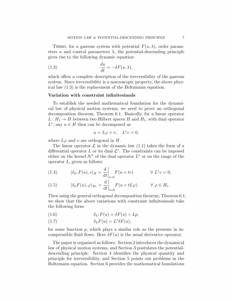
Third, for a gaseous system with potential F (u, λ), order param-eters u and control parameters λ, the potential-descending principlegives rise to the following dynamic equation:

(1.3)du

dt= −δF (u, λ),

which offers a complete description of the irreversibility of the gaseoussystem. Since irreversibility is a macroscopic property, the above phys-ical law (1.3) is the replacement of the Boltzmann equation.

Variation with constraint infinitesimals

To establish the needed mathematical foundation for the dynami-cal law of physical motion systems, we need to prove an orthogonaldecomposition theorem, Theorem 6.1. Basically, for a linear operatorL : H1 → H between two Hilbert spaces H and H1, with dual operatorL∗, any u ∈ H then can be decomposed as

u = Lϕ+ v, L∗v = 0,

where Lϕ and v are orthogonal in H.The linear operator L in the dynamic law (1.1) takes the form of a

differential operator L or its dual L∗. The constraints can be imposedeither on the kernel N ∗ of the dual operator L∗ or on the range of theoperator L, given as follows:

〈δL∗F (u), v〉H =d

dt

∣∣∣∣t=0

F (u+ tv) ∀ L∗v = 0,(1.4)

〈δLF (u), ϕ〉H1 =d

dt

∣∣∣∣t=0

F (u+ tLϕ) ∀ ϕ ∈ H1.(1.5)

Then using the general orthogonal decomposition theorem, Theorem 6.1,we show that the above variations with constraint infinitesimals takethe following form:

δL∗F (u) = δF (u) + Lp,(1.6)

δLF (u) = L∗δF (u),(1.7)

for some function p, which plays a similar role as the pressure in in-compressible fluid flows. Here δF (u) is the usual derivative operator.

The paper is organized as follows. Section 2 introduces the dynamicallaw of physical motion systems, and Section 3 postulates the potential-descending principle. Section 4 identifies the physical quantity andprinciple for irreversibility, and Section 5 points out problems in theBoltzmann equation. Section 6 provides the mathematical foundations

8 MA AND WANG

of the dynamical law of physical motion by proving the orthogonal-decomposition theorem and a theorem on variation with constraint-infinitesimals. Section 7 verifies the dynamical law of physical motionsby examining various important motion dynamical equations.

2. Dynamic Law of Physical Motion

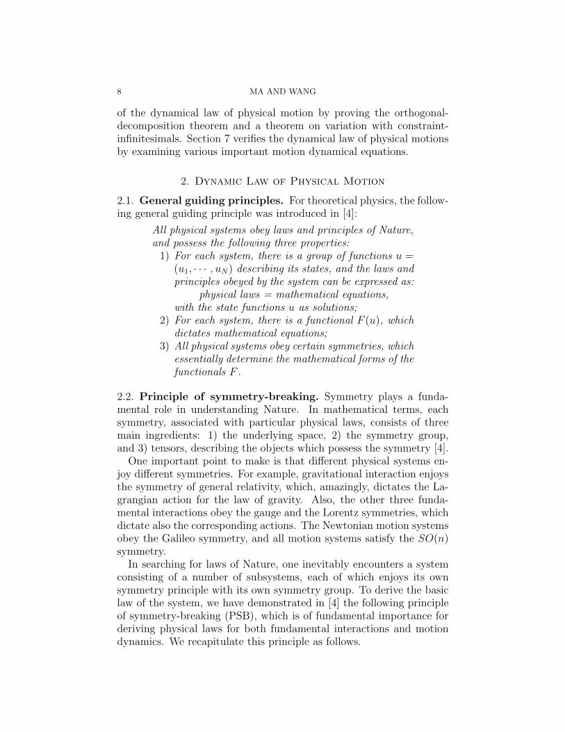
2.1. General guiding principles. For theoretical physics, the follow-ing general guiding principle was introduced in [4]:

All physical systems obey laws and principles of Nature,and possess the following three properties:

1) For each system, there is a group of functions u =(u1, · · · , uN) describing its states, and the laws andprinciples obeyed by the system can be expressed as:

physical laws = mathematical equations,with the state functions u as solutions;

2) For each system, there is a functional F (u), whichdictates mathematical equations;

3) All physical systems obey certain symmetries, whichessentially determine the mathematical forms of thefunctionals F .

2.2. Principle of symmetry-breaking. Symmetry plays a funda-mental role in understanding Nature. In mathematical terms, eachsymmetry, associated with particular physical laws, consists of threemain ingredients: 1) the underlying space, 2) the symmetry group,and 3) tensors, describing the objects which possess the symmetry [4].

One important point to make is that different physical systems en-joy different symmetries. For example, gravitational interaction enjoysthe symmetry of general relativity, which, amazingly, dictates the La-grangian action for the law of gravity. Also, the other three funda-mental interactions obey the gauge and the Lorentz symmetries, whichdictate also the corresponding actions. The Newtonian motion systemsobey the Galileo symmetry, and all motion systems satisfy the SO(n)symmetry.

In searching for laws of Nature, one inevitably encounters a systemconsisting of a number of subsystems, each of which enjoys its ownsymmetry principle with its own symmetry group. To derive the basiclaw of the system, we have demonstrated in [4] the following principleof symmetry-breaking (PSB), which is of fundamental importance forderiving physical laws for both fundamental interactions and motiondynamics. We recapitulate this principle as follows.


Principle 2.1 (PSB). Physical systems in different levels obey differentlaws, which are dictated by corresponding symmetries. For a systemcoupling different levels of physical laws, part of these symmetries mustbe broken:

1) There are several main symmetries- - the SO(n) invariance, theGalileo invariance, the Lorentz invariance, the SU(N) gaugeinvariance, and the general relativistic invariance– which aremutually independent and dictate in part the physical laws indifferent levels of Nature; and

2) for a system coupling several different physical laws, part ofthese symmetries must be broken.

2.3. Dynamic Law of Physical Motion. Theoretical physics stud-ies 1) the laws for the four fundamental interactions (gravity, electro-magnetism, the weak and the strong interactions), and 2) the laws formotion dynamics of physical systems.

According to their scales, physical systems are classified into

(1) classical mechanical systems (planetary scale),(2) quantum systems (micro level),(3) fluid mechanics systems,(4) astrophysical systems, and(5) statistical systems (relating microscopic properties of individual

particles to the macroscopic properties).

The basic laws for describing classical mechanical systems, quantumsystems and astrophysical systems are given in terms of Newtonianlaws, the principle of Lagrangian dynamics and the principle of Hamil-tonian dynamics. We shall see in Section 3 below that statistical phys-ical systems are described by the potential-descending principle. InSection 7, we show that fluid motion satisfies the dynamical law ofphysical motion introduced in the following.

By a careful examination of basic motion laws of different physicalsystems and by the mathematical study in Section 6 below, we discovera general dynamic law, suitable for all physical motion systems in (1)-(5) mentioned above.

To state this general dynamic law, we start with the definition ofconstraint variation. Let H,H1 be two Hilbert spaces, and

(2.1) L : H1 → H, L∗ : H → H∗1

be a pair of dual linear bounded operators. Consider a functionaldefined on H:

(2.2) F : H → R1.

10 MA AND WANG

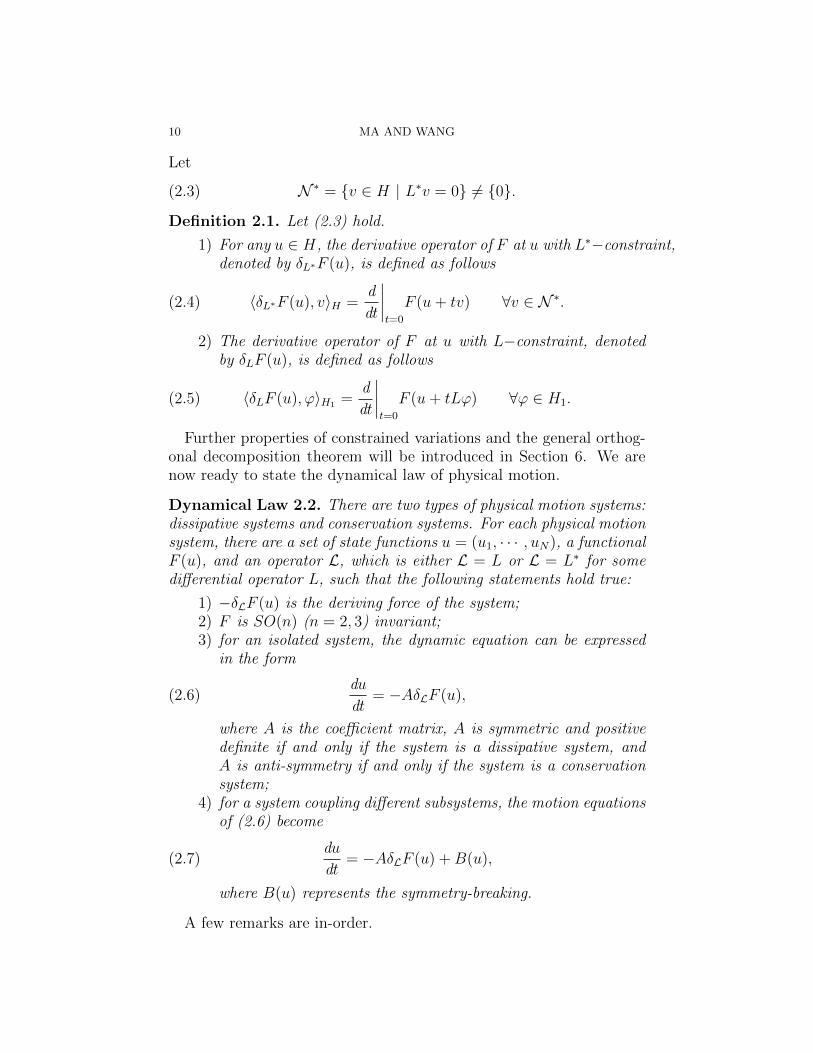
Let

(2.3) N ∗ = v ∈ H | L∗v = 0 6= 0.

Definition 2.1. Let (2.3) hold.

1) For any u ∈ H, the derivative operator of F at u with L∗−constraint,denoted by δL∗F (u), is defined as follows

(2.4) 〈δL∗F (u), v〉H =d

dt

∣∣∣∣t=0

F (u+ tv) ∀v ∈ N ∗.

2) The derivative operator of F at u with L−constraint, denotedby δLF (u), is defined as follows

(2.5) 〈δLF (u), ϕ〉H1 =d

dt

∣∣∣∣t=0

F (u+ tLϕ) ∀ϕ ∈ H1.

Further properties of constrained variations and the general orthog-onal decomposition theorem will be introduced in Section 6. We arenow ready to state the dynamical law of physical motion.

Dynamical Law 2.2. There are two types of physical motion systems:dissipative systems and conservation systems. For each physical motionsystem, there are a set of state functions u = (u1, · · · , uN), a functionalF (u), and an operator L, which is either L = L or L = L∗ for somedifferential operator L, such that the following statements hold true:

1) −δLF (u) is the deriving force of the system;2) F is SO(n) (n = 2, 3) invariant;3) for an isolated system, the dynamic equation can be expressed

in the form

(2.6)du

dt= −AδLF (u),

where A is the coefficient matrix, A is symmetric and positivedefinite if and only if the system is a dissipative system, andA is anti-symmetry if and only if the system is a conservationsystem;

4) for a system coupling different subsystems, the motion equationsof (2.6) become

(2.7)du

dt= −AδLF (u) +B(u),

where B(u) represents the symmetry-breaking.

A few remarks are in-order.


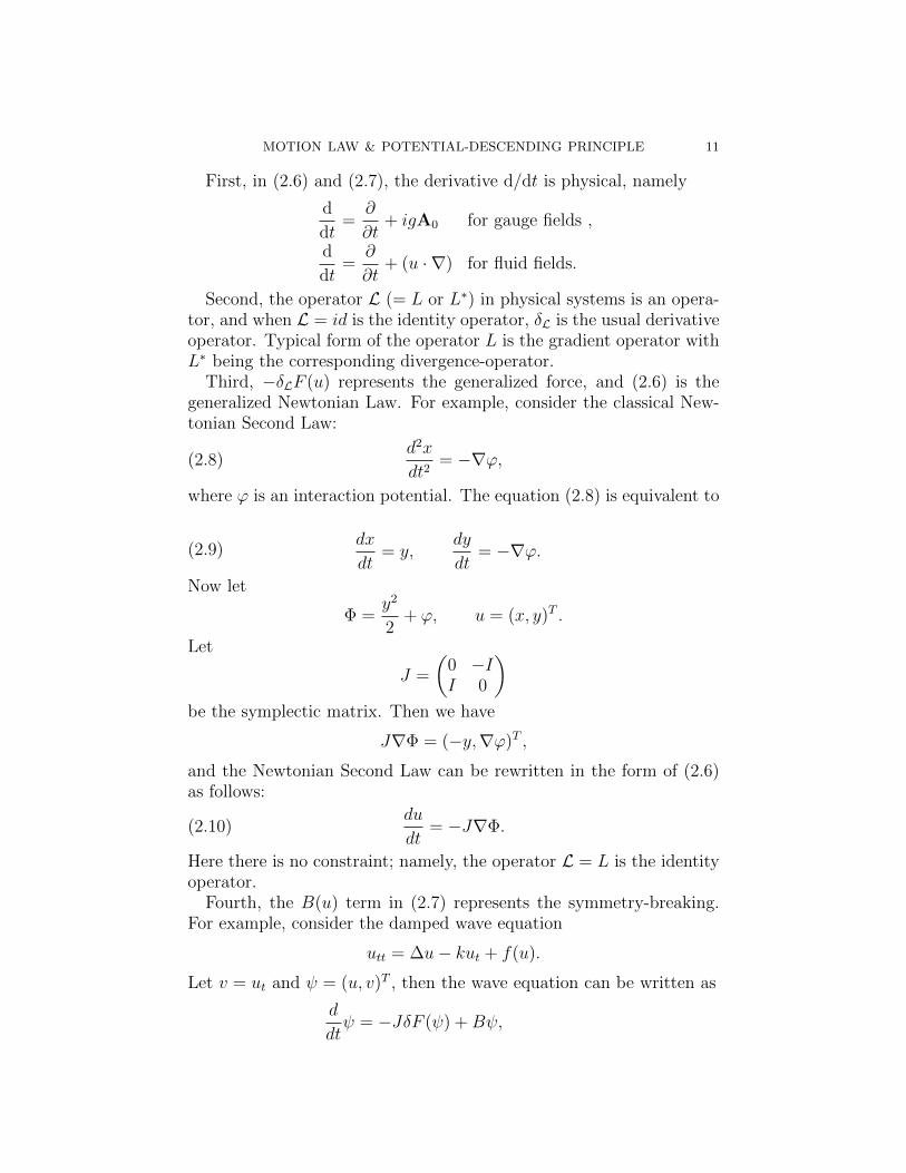
First, in (2.6) and (2.7), the derivative d/dt is physical, namely

d

dt=

∂

∂t+ igA0 for gauge fields ,

d

dt=

∂

∂t+ (u · ∇) for fluid fields.

Second, the operator L (= L or L∗) in physical systems is an opera-tor, and when L = id is the identity operator, δL is the usual derivativeoperator. Typical form of the operator L is the gradient operator withL∗ being the corresponding divergence-operator.

Third, −δLF (u) represents the generalized force, and (2.6) is thegeneralized Newtonian Law. For example, consider the classical New-tonian Second Law:

(2.8)d2x

dt2= −∇ϕ,

where ϕ is an interaction potential. The equation (2.8) is equivalent to

(2.9)dx

dt= y,

dy

dt= −∇ϕ.

Now let

Φ =y2

2+ ϕ, u = (x, y)T .

Let

J =

(0 −II 0

)be the symplectic matrix. Then we have

J∇Φ = (−y,∇ϕ)T ,

and the Newtonian Second Law can be rewritten in the form of (2.6)as follows:

(2.10)du

dt= −J∇Φ.

Here there is no constraint; namely, the operator L = L is the identityoperator.

Fourth, the B(u) term in (2.7) represents the symmetry-breaking.For example, consider the damped wave equation

utt = ∆u− kut + f(u).

Let v = ut and ψ = (u, v)T , then the wave equation can be written as

d

dtψ = −JδF (ψ) +Bψ,

12 MA AND WANG

F (ψ) =

∫ [1

2v2 + |∇u|2 +G(u)

],

Bψ =

(0−kv

).

Here the functional F inherits the symmetry of the wave equation with-out damping term kut. But the damping term cannot be included inthe functional F , and breaks the symmetry of the non-damped waveequation.

As mentioned earlier, symmetry-breaking is the essence for modelinga physical system coupling subsystems obeying different symmetries.

3. Potential-Descending Principle in Statistical Physics

In this section, we postulate the potential-descending principle (PDP)in statistical physics, which is more fundamental than the first and thesecond laws of thermodynamics. This principle also supports the dy-namic law of physical motion introduced in the last section.

3.1. Thermodynamic potentials. A thermodynamic system is de-scribed by order parameters (state functions), control parameters, andthermodynamic potential, which is a functional of the order parame-ters. There are four commonly used thermodynamic potentials: theinternal energy, the Helmholtz free energy, the Gibbs free energy, andthe enthalpy. The basic thermodynamic potential is the internal en-ergy, and the other three are derived using the Legendre transforms;see among others [6].

Conjugate pairs of state variables and internal energy. First, we notethat all thermodynamic potentials are expressed in terms of conjugatepairs. The most commonly considered conjugate thermodynamic vari-ables are

1) the temperature T and the entropy S, and2) f the generalized force and X the generalized displacement.

Typical examples of (f,X) include (the pressure p, the volumeV ), (applied magnetic field H, magnetization M), (applied elec-tric field E, electric polarization P ).

Let U be the internal energy. Then for a completely closed thermo-dynamic system, the first law states:

dU = TdS + fdX.(3.1)

Here (T, f) are the order parameters and (S,X) are the control param-eters.


Helmholtz energy. For an isothermal process, we need to use theHelmholtz free energy, denoted by

(3.2) F = U − TS.In fact, (3.2) is the Legendre transformation such that the Helmholtzfree energy F is a functional of S and f . In other words, (S, f) areorder parameters, and (T,X) are control parameters. Consequently,

F = F (S, f ;λ), λ = (T,X),

and the equilibrium state enjoys

(3.3)δF

δS= 0,

δF

δf= 0.

Gibbs free energy. When the system has the thermal and mechanicalexchanges with the external, i.e., the thermal process is in the constanttemperature T and generalized force f , the corresponding potential isthe Gibbs free energy, which is defined by

(3.4) G = F − fX, F the Helmholtz free energy,

which is the Legendre transformation regarding (T, f) as its indepen-dent variables. Namely, for the Gibbs potential, the order parametersare (S,X), and the control parameters are λ = (T, f),

G = G(S,X;λ),

and the equilibrium state satisfies

(3.5)δG

δS= 0,

δG

δX= 0.

3.2. Potential-Descending Principle in Statistical Physics. Wepostulate the following potential descending principle (PDP), and demon-strate in the remaining part of this paper that this principle serves asa fundamental principle in statistical physics.

Principle 3.1 (Potential-Descending Principle). For each thermody-namic system, there are order parameters u = (u1, · · · , uN), control pa-rameters λ, and the thermodynamic potential functional F (u;λ). For anon-equilibrium state u(t;u0) of the system with initial state u(0, u0) =u0, we have the following properties:

1) the potential F (u(t;u0);λ) is decreasing:

d

dtF (u(t;u0);λ) < 0 ∀t > 0;

2) the order parameters u(t;u0) have a limit

limt→∞

u(t;u0) = u;

14 MA AND WANG

3) there is an open and dense set O of initial data in the spaceof state functions, such that for any u0 ∈ O, the correspondingu is a minimum of F , which is called an equilibrium of thethermodynamic system:

δF (u;λ) = 0,

where δF represents the generalized force given in (2.6) and(2.7). Namely,

δF (u;λ) = −AδLF (u;λ).

3.3. Minimum potential principle. For an equilibrium state u of athermodynamic system, the potential-descending principle implies that

δ

δuF (u;λ) = 0,(3.6)

dF (u, λ) =∂F (u, λ)

∂λdλ.(3.7)

These are equilibrium equations of the system.For the equilibrium state, it is then easy to see that

dF (u, λ) =δ

δuF (u;λ)δu+

∂F

∂λdλ =

∂F (u;λ)

∂λdλ,

which is the first law of thermodynamics.For a given non-equilibrium thermodynamic state u(t), we have

dF (u(t), λ) =δ

δuF (u(t);λ)du+

∂F

∂λdλ.

The potential-descending principle tells us that

dF

dt=

δ

δuF (u(t);λ)

du

dt< 0.

As dt > 0, we then derive that

dF (u, λ) <∂F

∂λdλ,

which is the second law of thermodynamics.Also, as an example, we consider an internal energy of a thermody-

namic system, classical theory asserts that the first and second lawsare given by

(3.8) dU ≤ ∂U

∂SdS +

∂U

∂XdX,

where the equality represents the first laws, describing the equilibriumstate, and inequality presents second law for non-equilibrium state.However, there is a hidden assumption in (3.8) that at the equilibrium,


there is a free-variable in each of the conjugate pairs (T, S) and (f,X).In the internal energy system, S and X are free variables. Namely,

∂U

∂T≤ 0,

∂U

∂f≤ 0,

where, again, the equality is for equilibrium state and the strict inequal-ity is for non-equilibrium state. This assumption is mathematicallyequivalent to the minimal-potential principle (or potential-descendingprinciple).

In a nutshell, based on the above discussions, we have the followingimportant conclusion:

the potential-descending principle leads to both the firstand second law of thermodynamics, and the potential-descending principle is a more fundamental principlethen the first and second laws.

3.4. PDP-based mathematical models. Based on the principle,the dynamic equations of a thermodynamic system in non-equilibriumstate take the form

du

dt= −AδLF (u) for isolated systems,(3.9) du

dt= −AδLF (u) +B(u),∫AδLF (u) ·B(u) = 0

for coupled systems,(3.10)

where δL is the derivative operator with L− constraint for some op-erator L, B represents coupling operators, and A is a symmetric andpositive definite matrix of coefficients.

Consider a thermodynamic system involving a conserved order pa-rameter u:

(3.11)

∫Ω

u(x, t)dx = constant.

The potential is given by

(3.12) F = F1 − µ∫

Ω

udx,

where µ is the chemical potential, which plays the role of Lagrangianmultiplier, and F1 is the classical thermodynamical potential of the sys-tem. The key point here is that chemical potential cannot be regardedeither as an order parameter or as a control parameter for the ther-modynamic system. Consequently, the model based on the potential-descending principle is still given by (3.9) and (3.10).

16 MA AND WANG

It is important to remark that in [3] we used

∂uj∂t

= −∇ · Jj(u, λ),(3.13)

J = −k∇µ,(3.14)

µ =δF

δu,(3.15)

to derive the following dynamical equation; see [3, (3.1.21)]:

(3.16)∂u

∂t= ∆

δ

δuF (u, λ).

However, we realized in this article that the dynamical equation (3.16)(the model (3.1.21) in [3]), as well as the classical Cahn-Hilliard equa-tion, are incorrect. In fact, based on the Lagrangian multiplier theoremand by (3.11) and (3.15), we deduce that µ is the Lagrangian multiplier,which is a constant. Therefore, the relation (3.14) is invalid.

3.5. Diffusion and heat conductivity equation. Diffusion and heatconduction are properties of thermal systems. Their potential func-tional is written as

F =

∫Ω

[κ2|∇T |2 −QT

]dx,

where u represents the density for diffusion systems and the tempera-ture for heat conduction systems. Consequently, the dynamic equation

(3.17)dT

dt= −δF (T ).

is in the form:

(3.18)∂T

∂t= κ∆T +Q.

4. Irreversibility in Thermodynamic Systems

Natural phenomena show that the motion of all statistical physicalsystem (collection of large number of particles) possesses irreversibility.Namely, when the system evolves from one initial state to another, thesystem will not spontaneously return to its initial state without externalinterference. This phenomena is called (temporal) irreversibility.

Classical thermodynamics attributes this irreversibility to entropy-ascending principle. Based on the discussions in the previous sections,


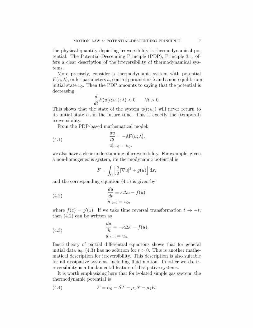
the physical quantity depicting irreversibility is thermodynamical po-tential. The Potential-Descending Principle (PDP), Principle 3.1, of-fers a clear description of the irreversibility of thermodynamical sys-tems.

More precisely, consider a thermodynamic system with potentialF (u, λ), order parameters u, control parameters λ and a non-equilibriuminitial state u0. Then the PDP amounts to saying that the potential isdecreasing:

d

dtF (u(t;u0);λ) < 0 ∀t > 0.

This shows that the state of the system u(t;u0) will never return toits initial state u0 in the future time. This is exactly the (temporal)irreversibility.

From the PDP-based mathematical model:

(4.1)

du

dt= −δF (u;λ),

u|t=0 = u0,

we also have a clear understanding of irreversibility. For example, givena non-homogeneous system, its thermodynamic potential is

F =

∫Ω

[κ2|∇u|2 + g(u)

]dx,

and the corresponding equation (4.1) is given by

(4.2)

du

dt= κ∆u− f(u),

u|t=0 = u0,

where f(z) = g′(z). If we take time reversal transformation t → −t,then (4.2) can be written as

(4.3)

du

dt= −κ∆u− f(u),

u|t=0 = u0.

Basic theory of partial differential equations shows that for generalinitial data u0, (4.3) has no solution for t > 0. This is another mathe-matical description for irreversibility. This description is also suitablefor all dissipative systems, including fluid motion. In other words, ir-reversibility is a fundamental feature of dissipative systems.

It is worth emphasizing here that for isolated simple gas system, thethermodynamic potential is

(4.4) F = U0 − ST − µ1N − µ2E,

18 MA AND WANG

where U0 is the internal energy, which is a constant, N is the numberof particles, µ1 and µ2 are Lagrangian multipliers, and E is the totalenergy. For this system, the entropy S is an order parameter, andtemperature T is a control parameter.

By (4.4), we see that potential-descending is equivalent to entropyascending:

d

dtF (S(t)) < 0 ⇐⇒ d

dtS(t) > 0.

In addition, according to the entropy formula:

S = k lnW,

and by the minimum potential principle:

δF = 0,

we can derive, with similar procedures as in [5, Section 6.1], all threedistributions: the Maxwell-Boltzmann distribution, the Fermi-Diracdistribution and the Bose-Einstein distribution. This shows that

the potential-descending principle is also the first prin-ciple of statistical mechanics.

5. Problems in Boltzmann Equation

5.1. Boltzmann equation. In statistical physics, a classical problemis how to establish a mathematical model that can faithfully describeirreversible processes. The Boltzmann equation is introduced mainlyfor this purpose. We start with a brief introduction on the derivationof the Boltzmann equation.

Consider a system of ideal gases that is in a non-equilibrium state,and assume its dynamical equation takes the form:

(5.1)dρ

dt= G(ρ),

where ρ stands for the probability density function of the gas molecules.By the general guiding principle of physics, (5.1) should be estab-

lished based on some fundamental laws and/or principles. Classicaltheories lack of such principles and laws. Therefore the Boltzmannequation is based on fulfilling the following two goals:

(1) Entropy-ascending principle: equation (5.1) should yield entropy-ascending property:

(5.2)d

dtS(ρ(t)) > 0,


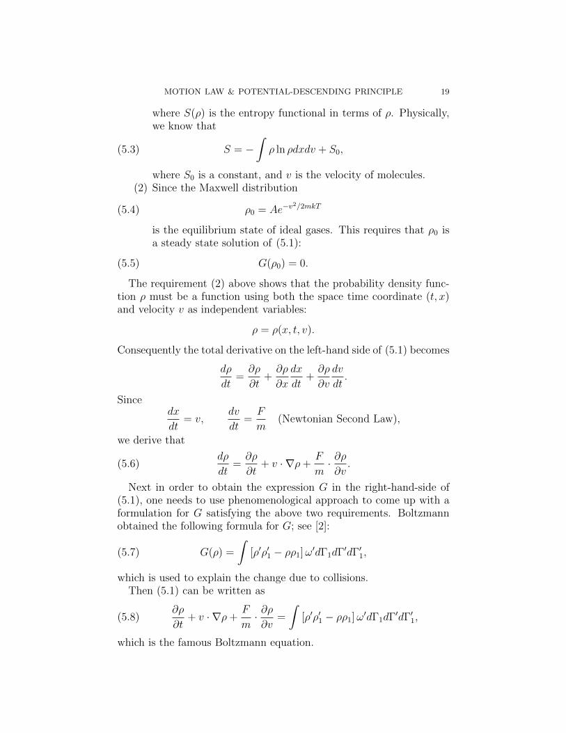
where S(ρ) is the entropy functional in terms of ρ. Physically,we know that

(5.3) S = −∫ρ ln ρdxdv + S0,

where S0 is a constant, and v is the velocity of molecules.(2) Since the Maxwell distribution

(5.4) ρ0 = Ae−v2/2mkT

is the equilibrium state of ideal gases. This requires that ρ0 isa steady state solution of (5.1):

(5.5) G(ρ0) = 0.

The requirement (2) above shows that the probability density func-tion ρ must be a function using both the space time coordinate (t, x)and velocity v as independent variables:

ρ = ρ(x, t, v).

Consequently the total derivative on the left-hand side of (5.1) becomes

dρ

dt=∂ρ

∂t+∂ρ

∂x

dx

dt+∂ρ

∂v

dv

dt.

Sincedx

dt= v,

dv

dt=F

m(Newtonian Second Law),

we derive that

(5.6)dρ

dt=∂ρ

∂t+ v · ∇ρ+

F

m· ∂ρ∂v.

Next in order to obtain the expression G in the right-hand-side of(5.1), one needs to use phenomenological approach to come up with aformulation for G satisfying the above two requirements. Boltzmannobtained the following formula for G; see [2]:

(5.7) G(ρ) =

∫[ρ′ρ′1 − ρρ1]ω′dΓ1dΓ′dΓ′1,

which is used to explain the change due to collisions.Then (5.1) can be written as

(5.8)∂ρ

∂t+ v · ∇ρ+

F

m· ∂ρ∂v

=

∫[ρ′ρ′1 − ρρ1]ω′dΓ1dΓ′dΓ′1,

which is the famous Boltzmann equation.

20 MA AND WANG

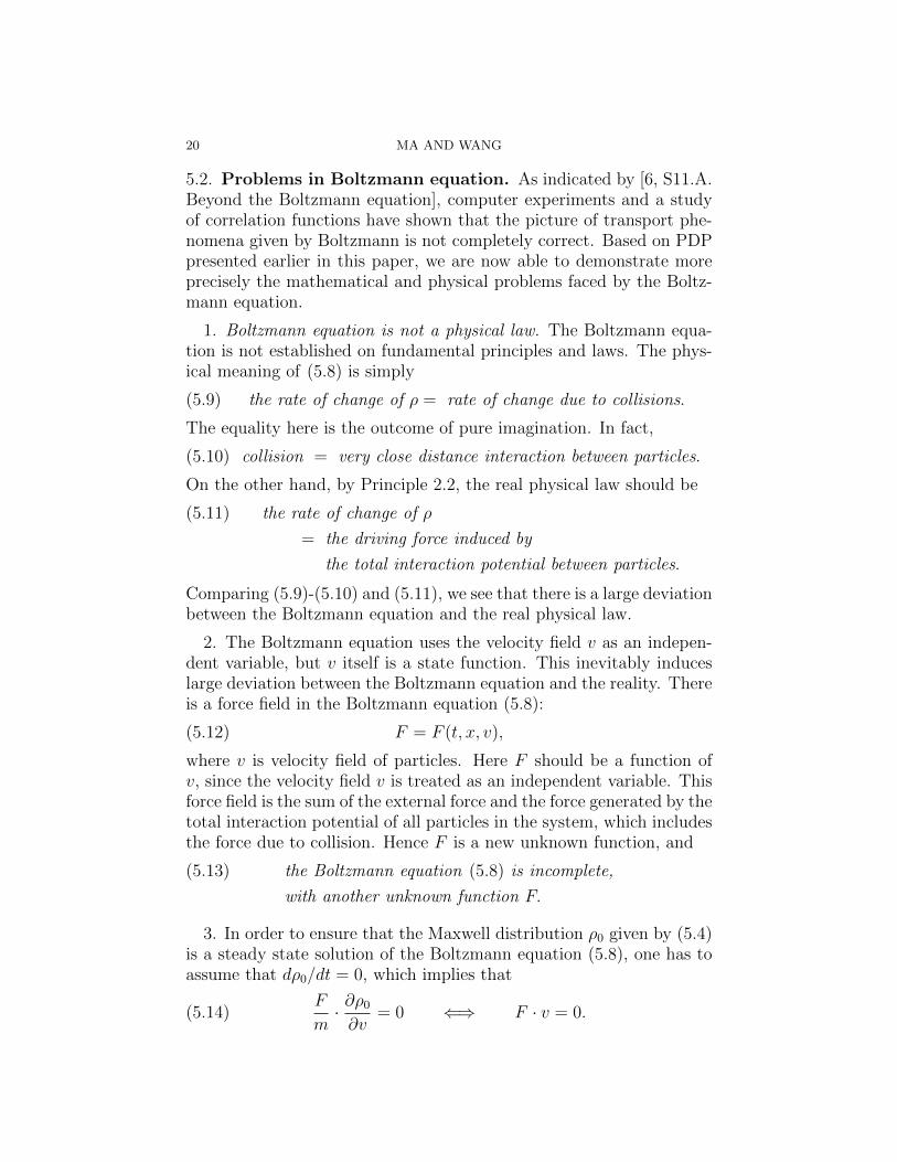
5.2. Problems in Boltzmann equation. As indicated by [6, S11.A.Beyond the Boltzmann equation], computer experiments and a studyof correlation functions have shown that the picture of transport phe-nomena given by Boltzmann is not completely correct. Based on PDPpresented earlier in this paper, we are now able to demonstrate moreprecisely the mathematical and physical problems faced by the Boltz-mann equation.

1. Boltzmann equation is not a physical law. The Boltzmann equa-tion is not established on fundamental principles and laws. The phys-ical meaning of (5.8) is simply

(5.9) the rate of change of ρ = rate of change due to collisions.

The equality here is the outcome of pure imagination. In fact,

(5.10) collision = very close distance interaction between particles.

On the other hand, by Principle 2.2, the real physical law should be

the rate of change of ρ(5.11)

= the driving force induced by

the total interaction potential between particles.

Comparing (5.9)-(5.10) and (5.11), we see that there is a large deviationbetween the Boltzmann equation and the real physical law.

2. The Boltzmann equation uses the velocity field v as an indepen-dent variable, but v itself is a state function. This inevitably induceslarge deviation between the Boltzmann equation and the reality. Thereis a force field in the Boltzmann equation (5.8):

(5.12) F = F (t, x, v),

where v is velocity field of particles. Here F should be a function ofv, since the velocity field v is treated as an independent variable. Thisforce field is the sum of the external force and the force generated by thetotal interaction potential of all particles in the system, which includesthe force due to collision. Hence F is a new unknown function, and

the Boltzmann equation (5.8) is incomplete,(5.13)

with another unknown function F.

3. In order to ensure that the Maxwell distribution ρ0 given by (5.4)is a steady state solution of the Boltzmann equation (5.8), one has toassume that dρ0/dt = 0, which implies that

(5.14)F

m· ∂ρ0

∂v= 0 ⇐⇒ F · v = 0.


This requires that

(5.15) F = 0.

This assumption (5.15) is non-physical, since under (5.15), all particlesin the system, with zero force, will make uniform rectilinear motion.This is in contradiction with the reality, and leads to the followinginconsistency of the Boltzmann equation with the real phenomena:

(5.16)

the Maxwell distribution (5.4) is a steady state solution

of the Boltzmann equation (5.8) under

the non-physical assumption (5.15).

4. In deriving the H-Theorem (i.e. the entropy-ascending principle),the following must be assumed:

(5.17) F = F (t, x) is independent of v.

However, the Boltzmann equation (5.8) treats the velocity v as anindependent variable. In this case, the force field F must be treatedas a function of v as well. Consequently the above assumption (5.17)is rather arbitrary, and any model using velocity v as an independentvariable is inconsistent with the assumption (5.17). In other words, theH-Theorem is not a natural consequence of the Boltzmann equation(5.8).

Remark 5.1. In statistical physics, one often regards the Boltzmannequation as a model only suitable for dilute ideal gas. The misperceptionis that the mutual interaction between particles in a dilute gas systemis negligible, leading to the assumption F = 0 in (5.15). However, theforce field generated by the total interaction potential Φ of all particles:

(5.18) F = −∇Φ

is not small, and is not simply measured by r−2 between particles. Themotion of particles in any dilute gas system is chaotic, and the ve-locities of the particles are not small even when there is no externalforce present. Consequently, the interaction force field is not small,and cannot simply be ignored.

5. Ignoring the non-physical nature of assumption (5.15), the spaceof all steady state solutions of the Boltzmann equation (5.8) have 5-dimension. Namely, the general form of the steady state solutions is

ρ = eα0+α1v1+α2v2+α3v3+α4v2 ,

22 MA AND WANG

where αi (i = 0, · · · , 4) are constants, and v = (v1, v2, v3). This showsthat each steady-state is not stable, and this does not fit the reality.

6. Entropy-decreasing principle shows that a gaseous system in theequilibrium has the maximum entropy, i.e. the Maxwell distribution(5.4) should be the maximum of (5.3). However, the maximum of (5.3)is given by

ρ0 = e−1.

Again, this is non-physical.

5.3. Conclusions. In a nutshell, the above discussions clearly demon-strate the following conclusions:

1. Laws of physics (equations) should not use state functions as in-dependent variables, which are themselves governed by physical laws.The Boltzmann equation violates this simple physical rule, and there-fore is not able to faithfully reflect the true nature of the underlyingphysical phenomena.

2. Irreversibility is a common characteristic of all dissipative systems,and is not an entropy property. The Potential-Descending Principleintroduced in this paper is the basic mathematical model/descriptionof irreversibility.

3. The Boltzmann equation was aimed to develop a mathematicalmodel for entropy-increasing principle. This is an incorrect startingpoint, since thermodynamic potential is the right physical quantityfor the mathematical characterization of irreversibility, rather than en-tropy.

4. Let F (u, λ) be the thermodynamic potential of a gaseous systemwith order parameters u and control parameters λ. Then PDP givesrise to the following dynamic equation:

(5.19)du

dt= −δF (u, λ).

This equation offers a complete description of the irreversibility of thegaseous system.

6. Mathematical Foundations of Dynamic Law

6.1. General orthogonal Decomposition Theorem. The follow-ing is a general orthogonal decomposition theorem. Let X be a linearspace, H be a Hilbert space, and

L : X → H be a linear map.


Let

N = ϕ ∈ X | Lϕ = 0,be the kernel of L, and let H1 be the completion of X/N with thefollowing norm

(6.1) ||ϕ||2H1= 〈Lϕ,Lϕ〉H , ϕ ∈ X/N .

It is clear that H1 is a Hilbert space, and

(6.2)L : H1 → H is bounded,

L∗ : H → H∗1 is the dual operator of L.

Then we have the L−orthogonal decomposition theorem as follows.

Theorem 6.1 (L-Orthogonal Decomposition Theorem). For the linearoperators L and L∗ in (6.2) and any u ∈ H, there exists a ϕ ∈ H1 andv ∈ H, such that u can be decomposed as

(6.3) u = Lϕ+ v, L∗v = 0, 〈Lϕ, v〉H = 0.

Proof. For a given u ∈ H, consider the existence of the equation

(6.4) L∗Lϕ = L∗u,

for solution ϕ ∈ H1. By (6.1) we can see that the operator

A = L∗L : H1 → H∗1 ,

is positive definition, i.e., for any ψ ∈ H1 we have

〈Aψ,ψ〉H1 = 〈Lψ,Lψ〉H = ||ψ||2H1.

Therefore, by the Lax-Milgram theorem, the equation (6.4) has a uniquesolution ϕ ∈ H1. Then we take

(6.5) v = u− Lϕ ∈ H.

By (6.4) we see that

(6.6) L∗v = 0.

Thus, (6.5) is the decomposition of (6.4), and by (6.6) we have

〈Lϕ, v〉H = 〈ϕ,L∗v〉H1 = 0,

i.e., Lϕ and v are orthogonal in H. The proof is complete.

We demonstrate the applications of the above theorem with twoexamples.

24 MA AND WANG

Example 6.1. Let H = L2(Ω,Rn) be the space of all n-dimensionalvector fields defined on an open set Ω ⊂ Rn, and

H1 = H1(Ω)/R =

ϕ ∈ H1(Ω) |

∫Ω

ϕdx = 0

.

Let

(6.7) L = ∇ : H1 → H be the gradient operator,

and the duality L∗ : H → H∗1 is as follows

(6.8) 〈L∗v, ϕ〉H1 =

∫Ω

(−divv)ϕdx+

∫∂Ω

ϕv · nds

∀ϕ ∈ H1. By (6.8) we can see that

(6.9) L∗v = 0⇐⇒ divv = 0, v · n|∂Ω = 0.

Therefore, for the operators (6.7) and (6.9) the vector fields u in H =L2(Ω,Rn) can be decomposed as

(6.10) u = ∇ϕ+ v, div v = 0, v · n|∂Ω = 0.

This is the Leray decomposition.

Example 6.2. The decomposition of the tensor in Riemannian man-ifolds. Let M be a n−dimensional manifold without boundary, andH = L2(T krM) be the space consisting of square integrable (k, r)-tensoron M , and

H1 = H1(T k−1r M) (or H1(T kr−1M)).

For the gradient operator

L = ∇ : H1 → H,

the dual operator is the divergent operator

L∗ = div : H → H∗1 .

By Theorem 6.1, for u ∈ H = L2(T krM) we have

(6.11) u = ∇ϕ+ v, divv = 0, ϕ ∈ H1.

6.2. Variations with constrained-infinitesimals. LetH,H1 be twoHilbert spaces, and

(6.12) L : H1 → H, L∗ : H → H∗1

be a pair of dual linear bounded operators. Consider the functionalsdefined on H, i.e.,

(6.13) F : H → R1.

Then we introduce the following definitions. Let

(6.14) N ∗ = v ∈ H | L∗v = 0 6= 0,


i.e., dim N ∗ > 0.We now recall the notion of constraint variations given in Defini-

tion 2.1:

1) For any u ∈ H, the derivative operator of F at u with L∗−constraint,denoted by δL∗F (u), is defined as follows

(6.15) 〈δL∗F (u), v〉H =d

dt

∣∣∣∣t=0

F (u+ tv) ∀v ∈ N ∗.

2) The derivative operator of F at u with L−constraint, denotedby δLF (u), is defined as follows

(6.16) 〈δLF (u), ϕ〉H1 =d

dt

∣∣∣∣t=0

F (u+ tLϕ) ∀ϕ ∈ H1.

The following theorem is based on Theorem 6.1.

Theorem 6.2 (Variation with L−constraints). For the variationalderivatives with L∗ and L constraints defined in (6.15) and (6.16) wehave the following conclusions.

1) For δL∗F (u), there is a ϕ ∈ H1 such that

(6.17) δL∗F (u) = δF (u) + Lϕ.

2) For δLF (u), we have

(6.18) δLF (u) = L∗δF (u).

Here δF (u) is the normal derivative operator.

Proof. The theorem follows from Definition 2.1 and Theorem 6.1. Infact, by definition, we have

〈δL∗F (u), v〉H = 〈δF (u), v〉 ∀L∗v = 0,

which, by Theorem 6.1, implies (6.17).Also, by definition, we have

〈δLF (u), ϕ〉H1 = 〈δF (u), Lϕ〉H = 〈L∗δLF (u), ϕ〉H1 ,

which leads to (6.18).

By Theorem 6.2, we shall show that all physical motion systems,without coupling to other systems, have a functional

F : H → R1

such that the dynamical equations of the systems can be expressed as

(6.19)du

dt= −AδLF (u),

26 MA AND WANG

where A is a coefficient matrix, δLF (u) is the derivative operator ofF at u with L−constraint. Note that the normal derivative operatorδF (u) correspond to δLF (u) with L = id the identity.

7. Dynamics of Other Physical Motion Systems

7.1. Newtonian laws. A group of bodies with masses (m1, · · · ,mN)motion in a potential field V (x), the motion equations are

(7.1)dpidt

= −miδiV (x) (1 ≤ i ≤ N),

where δi = ∂/∂xi. In (2.8), we have shown that (7.1) has the form of(2.6).

Consider the electron motion equation given by

(7.2) mdv

dt= eE +

e

cv ×H.

Based on the electromagnetic theory,

momentum of electron p = mv +e

cA,

electromagnetic potential Φ = ϕ− 1

cA · v.

Then (7.2) is equivalent to the equation (see Landau and Lifshitz [1]):

(7.3)dp

dt= −e∇Φ,

which can be equivalently written as

du

dt= −JδΨ,

where u = (x, p)T , and

Ψ =1

2mp2 − e

mcA · p+

e

cA2 + eϕ,

J =

(0 −II 0

).

7.2. Fluid Dynamics. We consider here two examples–the compress-ible Navier-Stokes equations and the Boussinesq equations.


We start with the compressible Navier-Stokes equations:

(7.4)

∂u

∂t+ (u · ∇)u =

1

ρ[µ∆u−∇p+ f ] ,

∂ρ

∂t= −div (ρu)

u|∂Ω = 0.

Let the constraint operator L = −∇ be the gradient operator, withdual operator L∗ = div. Also, let

Φ(u, ρ) =

∫Ω

[µ

2|∇u|2 − fu+

1

2ρ2divu

]dx.

Then the equations of (7.4) are written as

(7.5)

du

dt= −1

ρ

δL∗

δuΦ(u, ρ),

dρ

dt= − δ

δρΦ(u, ρ),

which is in the form of (2.6) with coefficient matrix A = diag(1/ρ, 1).Also, the pressure is given by

p = p0 − λdivu− 1

2ρ2.

Here

du

dt=∂u

∂t+∂u

∂xi

dxidt

=∂u

∂t+ (u · ∇)u,

dρ

dt=∂ρ

∂t+ u · ∇ρ.

The Boussinesq equations are written as

(7.6)

∂u

∂t+ (u · ∇)u− ρ−1

0 [ν∆u+∇p] = −gkρ(T ),

∂T

∂t+ (u · ∇)T − κ∆T = 0,

divu = 0,

where ν, κ, g are constants, u = (u1, u2, u3) is the velocity field, p isthe pressure function, T is the temperature function, T0 is a constantrepresenting the lower surface temperature at x3 = 0, and k = (0, 0, 1)is the unit vector in the x3-direction.

As before, we take the linear constraint operator L = −∇ with dualL∗ = div. Let

Φ(u, T ) =

∫Ω

[µ2|∇u|2 +

κ

2|∇T |2

]dx.

28 MA AND WANG

Then the Boussinesq equations of (7.6) are written as

(7.7)

du

dt= − 1

ρ0

δL∗

δuΦ(u, T ) +B(u, T ),

dT

dt= − δ

δTΦ(u, T ),

which is in the form of (2.6) with coefficient matrix A = diag(1/ρ0, 1).The term B(u, T ) is given by

B(u, T ) = gρ0kρ(T ),

which breaks the symmetry of the functional Φ(u, T ), caused by thecoupling between momentum equations and the temperature equation.Also, the incompressibility condition div u = 0 is built into the con-struction of the basic function space, which we omit the details.

7.3. Hamiltonian dynamics. The principe of Hamiltonian dynamics(PHD) is a universal principle, which governs all energy conservativesystems, including the astronomic mechanics, wave motion equations,quantum mechanics, and the Maxwell equations.

PHD amounts to saying that for a conservative system, there aretwo sets of conjugate functions u = (u1, · · · , uN), v = (v1, · · · , vN)and a Hamiltonian energy H = H(u, v), such that u and v satisfy theequations; see among others Ma and Wang [4]:

∂u

∂t= k

δ

δvH(u, v),

∂v

∂t= −k δ

δuH(u, v),

which can be expressed in form of (2.6) as

(7.8)dv

dt= −AδH(u, v),

where

A = k

(0 −II 0

)is an anti-symmetric matrix.

7.4. Lagrangian Dynamics. The principle of Lagrangian dynamics(PLD) is also a universal principle in physics, which governs the phys-ical motion systems such as Newtonian mechanics, quantum physicalsystem, elastic waves, classical electrodynamics etc; see among others[1, 4].


PLD amounts to saying that for an isolated motion system, thereare state functions u = (u1, · · · , uN) and a functional F (u) called theLagrangian action, such that u satisfies

(7.9) δF (u) = 0,

which can be equivalently referred to the Hamiltonian system (7.8)with conjugates u and v = ut.

References

[1] L. D. Landau and E. M. Lifshitz, Course of theoretical physics, Vol. 2,Pergamon Press, Oxford, fourth ed., 1975. The classical theory of fields, Trans-lated from the Russian by Morton Hamermesh.

[2] E. M. Lifschitz and L. P. Pitajewski, Lehrbuch der theoretischen Physik(“Landau-Lifschitz”). Band X, Akademie-Verlag, Berlin, second ed., 1990.Physikalische Kinetik. [Physical kinetics], Translated from the Russian by GerdRopke and Thomas Frauenheim, Translation edited and with a foreword byPaul Ziesche and Gerhard Diener.

[3] T. Ma and S. Wang, Phase Transition Dynamics, Springer-Verlag, 2013.[4] , Mathematical Principles of Theoretical Physics, Science Press, 2015.[5] R. K. Pathria and P. D. Beale, Statistical Mechanics, Elsevier, third ed.,

2011.[6] L. E. Reichl, A modern course in statistical physics, A Wiley-Interscience

Publication, John Wiley & Sons Inc., New York, second ed., 1998.

(TM) Department of Mathematics, Sichuan University, Chengdu, P.R. China

E-mail address: [email protected]

(SW) Department of Mathematics, Indiana University, Bloomington,IN 47405

E-mail address: [email protected]

dynamic law of physical motion and

Documents