Dynamic Language Models for Streaming Text

Dani Yogatama∗ Chong Wang∗ Bryan R. Routledge† Noah A. Smith∗ Eric P. Xing∗∗School of Computer Science†Tepper School of BusinessCarnegie Mellon UniversityPittsburgh, PA 15213, USA

∗{dyogatama,chongw,nasmith,epxing}@cs.cmu.edu, †routledge@cmu.edu

AbstractWe present a probabilistic language model thatcaptures temporal dynamics and conditions onarbitrary non-linguistic context features. Thesecontext features serve as important indicatorsof language changes that are otherwise difficultto capture using text data by itself. We learnour model in an efficient online fashion that isscalable for large, streaming data. With fivestreaming datasets from two different genres—economics news articles and social media—weevaluate our model on the task of sequentiallanguage modeling. Our model consistentlyoutperforms competing models.

1 Introduction

Language models are a key component in many NLPapplications, such as machine translation and ex-ploratory corpus analysis. Language models are typi-cally assumed to be static—the word-given-contextdistributions do not change over time. Examplesinclude n-gram models (Jelinek, 1997) and proba-bilistic topic models like latent Dirichlet allocation(Blei et al., 2003); we use the term “language model”to refer broadly to probabilistic models of text.

Recently, streaming datasets (e.g., social media)have attracted much interest in NLP. Since such dataevolve rapidly based on events in the real world, as-suming a static language model becomes unrealistic.In general, more data is seen as better, but treating allpast data equally runs the risk of distracting a modelwith irrelevant evidence. On the other hand, cau-tiously using only the most recent data risks overfit-ting to short-term trends and missing important time-insensitive effects (Blei and Lafferty, 2006; Wanget al., 2008). Therefore, in this paper, we take stepstoward methods for capturing long-range temporaldynamics in language use.

Our model also exploits observable context vari-ables to capture temporal variation that is otherwisedifficult to capture using only text. Specifically forthe applications we consider, we use stock marketdata as exogenous evidence on which the languagemodel depends. For example, when an importantcompany’s price moves suddenly, the language modelshould be based not on the very recent history, butshould be similar to the language model for a daywhen a similar change happened, since people arelikely to say similar things (either about that com-pany, or about conditions relevant to the change).Non-linguistic contexts such as stock price changesprovide useful auxiliary information that might indi-cate the similarity of language models across differ-ent timesteps.

We also turn to a fully online learning framework(Cesa-Bianchi and Lugosi, 2006) to deal with non-stationarity and dynamics in the data that necessitateadaptation of the model to data in real time. In on-line learning, streaming examples are processed onlywhen they arrive. Online learning also eliminatesthe need to store large amounts of data in memory.Strictly speaking, online learning is distinct fromstochastic learning, which for language models builton massive datasets has been explored by Hoffmanet al. (2013) and Wang et al. (2011). Those tech-niques are still for static modeling. Language model-ing for streaming datasets in the context of machinetranslation was considered by Levenberg and Os-borne (2009) and Levenberg et al. (2010). Goyalet al. (2009) introduced a streaming algorithm forlarge scale language modeling by approximating n-gram frequency counts. We propose a general onlinelearning algorithm for language modeling that drawsinspiration from regret minimization in sequentialpredictions (Cesa-Bianchi and Lugosi, 2006) and on-

181

Transactions of the Association for Computational Linguistics, 2 (2014) 181–192. Action Editor: Eric Fosler-Lussier.Submitted 10/2013; Revised 2/2014; Published 4/2014. c©2014 Association for Computational Linguistics.

line variational algorithms (Sato, 2001; Honkela andValpola, 2003).

To our knowledge, our model is the first to bringtogether temporal dynamics, conditioning on non-linguistic context, and scalable online learning suit-able for streaming data and extensible to includetopics and n-gram histories. The main idea of ourmodel is independent of the choice of the base lan-guage model (e.g., unigrams, bigrams, topic models,etc.). In this paper, we focus on unigram and bi-gram language models in order to evaluate the basicidea on well understood models, and to show how itcan be extended to higher-order n-grams. We leaveextensions to topic models for future work.

We propose a novel task to evaluate our proposedlanguage model. The task is to predict economics-related text at a given time, taking into account thechanges in stock prices up to the corresponding day.This can be seen an inverse of the setup consideredby Lavrenko et al. (2000), where news is assumedto influence stock prices. We evaluate our modelon economics news in various languages (English,German, and French), as well as Twitter data.

2 Background

In this section, we first discuss the background forsequential predictions then describe how to formulateonline language modeling as sequential predictions.

2.1 Sequential Predictions

Let w1, w2, . . . , wT be a sequence of response vari-ables, revealed one at a time. The goal is to designa good learner to predict the next response, givenprevious responses and additional evidence whichwe denote by xt ∈ RM (at time t). Throughout thispaper, we use the term features for x. Specifically, ateach round t, the learner receives xt and makes a pre-diction wt, by choosing a parameter vectorαt ∈ RM .In this paper, we refer to α as feature coefficients.

There has been an enormous amount of work ononline learning for sequential predictions, much of itbuilding on convex optimization. For a sequence ofloss functions `1, `2, . . . , `T (parameterized by α),an online learning algorithm is a strategy to minimizethe regret, with respect to the best fixed α∗ in hind-sight.1 Regret guarantees assume a Lipschitz con-

1Formally, the regret is defined as RegretT (α∗) =

dition on the loss function ` that can be prohibitivefor complex models. See Cesa-Bianchi and Lugosi(2006), Rakhlin (2009), Bubeck (2011), and Shalev-Shwartz (2012) for in-depth discussion and review.

There has also been work on online and stochasticlearning for Bayesian models (Sato, 2001; Honkelaand Valpola, 2003; Hoffman et al., 2013), based onvariational inference. The goal is to approximate pos-terior distributions of latent variables when examplesarrive one at a time.

In this paper, we will use both kinds of techniquesto learn language models for streaming datasets.

2.2 Problem FormulationConsider an online language modeling problem, inthe spirit of sequential predictions. The task is tobuild a language model that accurately predicts thetexts generated on day t, conditioned on observ-able features up to day t, x1:t. Every day, afterthe model makes a prediction, the actual texts wt

are revealed and we suffer a loss. The loss is de-fined as the negative log likelihood of the model`t = − log p(wt | α,β1:t−1,x1:t−1,n1:t−1), whereα and β1:T are the model parameters andn is a back-ground distribution (details are given in §3.2). Wecan then update the model and proceed to day t+ 1.Notice the similarity to the sequential prediction de-scribed above. Importantly, this is a realistic setup forbuilding evolving language models from large-scalestreaming datasets.

3 Model

3.1 NotationWe index timesteps by t ∈ {1, . . . , T} and wordtypes by v ∈ {1, . . . , V }, both are always given assubscripts. We denote vectors in boldface and use1 : T as a shorthand for {1, 2, . . . , T}. We assumewords of the form {wt}Tt=1 for wt ∈ RV , which isthe vector of word frequences at timetstep t. Non-linguistic context features are {xt}Tt=1 for xt ∈ RM .The goal is to learn parameters α and β1:T , whichwill be described in detail next.

3.2 Generative StoryThe main idea of our model is illustrated by the fol-lowing generative story for the unigram languagePT

t=1 `t(xt,αt, wt)− infα∗PT

t=1 `t(xt,α∗, wt).

182

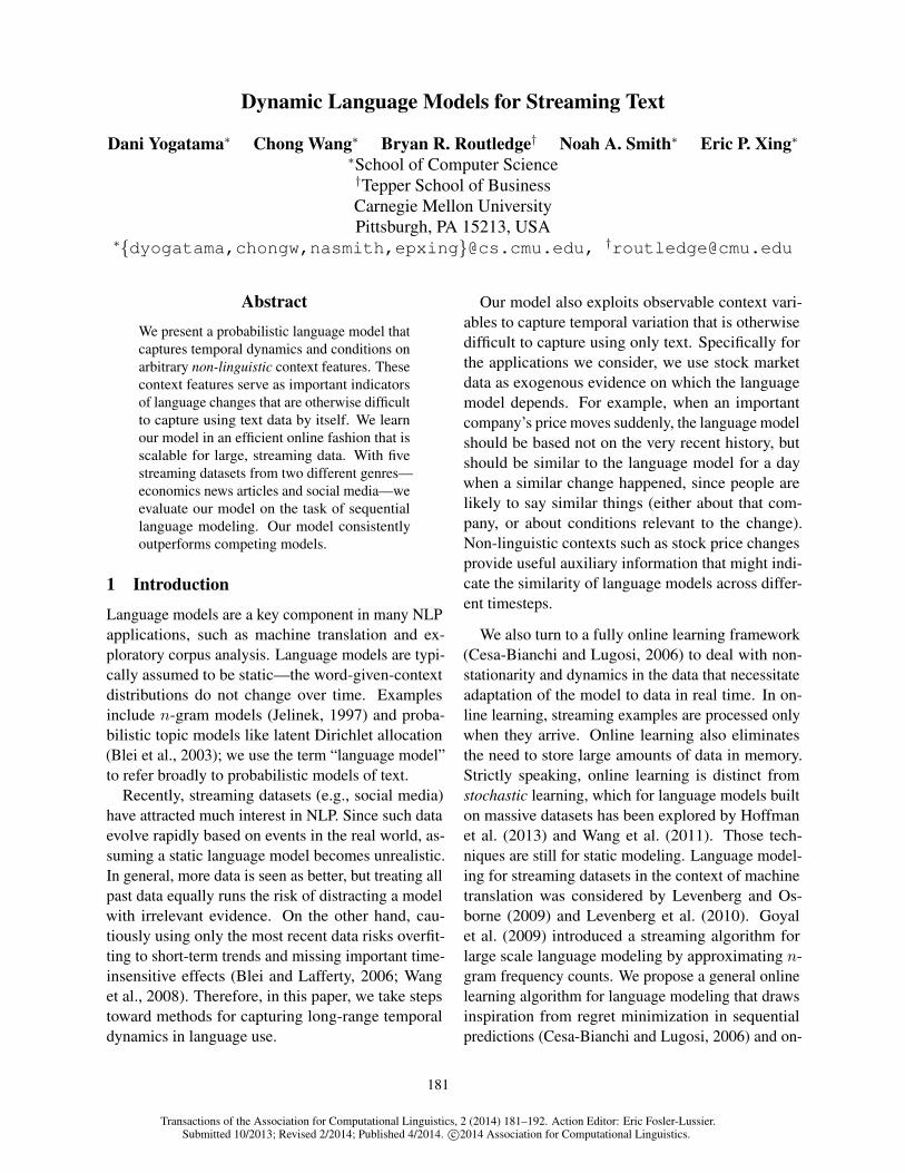
model. (We will discuss the extension to higher-orderlanguage models later.) A graphical representationof our proposed model is given in Figure 1.

1. Draw feature coefficients α ∼ N(0, λI).2 Hereα is a vector in RM , where M is the dimension-ality of the feature vector.

2. For each timestep t:(a) Observe non-linguistic context features xt.(b) Draw βt ∼

N

(∑t−1k=1 δk

exp(α>f(xt,xk))Pt−1j=1 δj exp(α

>f(xt,xj))βk, ϕI

).

Here, βt is a vector in RV , where V isthe size of the word vocabulary, ϕ isthe variance parameter and δk is a fixedhyperparameter; we discuss them below.

(c) For each word wt,v, draw wt,v ∼Categorical

(exp(n1:t−1,v+βt,v)P

j∈V exp(n1:t−1,j+βt,j)

).

In the last step, βt and n are mapped to the V -dimensional simplex, forming a distribution overwords. n1:t−1 ∈ RV is a background (log) distri-bution, inspired by a similar idea in Eisenstein et al.(2011). In this paper, we set n1:t−1,v to be the log-frequency of v up to time t− 1. We can interpret βas a time-dependent deviation from the backgroundlog-frequencies that incorporates world-context. Thisdeviation comes in the form of a weighted average ofearlier deviation vectors.

The intuition behind the model is that the probabil-ity of a word appearing at day t depends on the back-ground log-frequencies, the deviation coefficients ofthe word at previous timesteps β1:t−1, and the sim-ilarity of current conditions of the world (based onobservable features x) to previous timesteps throughf(xt,xk). That is, f is a function that takes d-dimensional feature vectors at two timesteps xt andxk and returns a similarity vector f(xt,xk) ∈ RM(see §6.1.1 for an example of f that we use in ourexperiments). The similarity is parameterized by α,and decays over time with rate δk. In this work, weassume a fixed window size c (i.e., we consider cmost recent timesteps), so that δ1:t−c−1 = 0 andδt−c:t−1 = 1. This allows up to cth order depen-dencies.3 Setting δ this way allows us to bound the

2Feature coefficients α can be also drawn from other distri-butions such as α ∼ Laplace(0, λ).

3In online Bayesian learning, it is known that forgettinginaccurate estimates from earlier timesteps is important (Sato,

�

xtxsxrxq

wq wr ws wt

�t�s�r�q

↵

NrNq NsNt

T

Figure 1: Graphical representation of the model. Thesubscript indices q, r, s are shorthands for the previ-ous timesteps t − 3, t − 2, t − 1. Only four timestepsare shown here. There are arrows from previousβt−4,βt−5, . . . ,βt−c to βt, where c is the window sizeas described in §3.2. They are not shown here, for read-ability.

number of past vectors β that need to be kept inmemory. We set β0 to 0.

Although the generative story described aboveis for unigram language models, extensions can bemade to more complex models (e.g., mixture of un-igrams, topic models, etc.) and to longer n-gramcontexts. In the case of topic models, the modelwill be related to dynamic topic models (Blei andLafferty, 2006) augmented by context features, andthe learning procedure in §4 can be used to performonline learning of dynamic topic models. However,our model captures longer-range dependencies thandynamic topic models, and can condition on non-linguistic features or metadata. In the case of higher-order n-grams, one simple way is to draw more β,one for each history. For example, for a bigrammodel, β is in RV 2

, rather than RV in the unigrammodel. We consider both unigram and bigram lan-guage models in our experiments in §6. However, themain idea presented in this paper is largely indepen-dent of the base model.

Related work. Mimno and McCallum (2008) andEisenstein et al. (2010) similarly conditioned text on

2001; Honkela and Valpola, 2003). Since we set δ1:t−c−1 = 0,at every timestep t, δk leads to forgetting older examples.

183

observable features (e.g., author, publication venue,geography, and other document-level metadata), butconducted inference in a batch setting, thus their ap-proaches are not suitable for streaming data. It is notimmediately clear how to generalize their approach todynamic settings. Algorithmically, our work comesclosest to the online dynamic topic model of Iwataet al. (2010), except that we also incorporate contextfeatures.

4 Learning and Inference

The goal of the learning procedure is to minimize theoverall negative log likelihood,

− logL(D) =

− log

∫dβ1:T p(β1:T | α,x1:T )p(w1:T | β1:T ,n).

However, this quantity is intractable. Instead, wederive an upper bound for this quantity and minimizethat upper bound. Using Jensen’s inequality, the vari-ational upper bound on the negative log likelihoodis:

− logL(D) ≤ −∫dβ1:T q(β1:T | γ1:T ) (4)

logp(β1:T | α,x1:T )p(w1:T | β1:T ,n)

q(β1:T | γ1:T ).

Specifically, we use mean-field variational inferencewhere the variables in the variational distribution qare completely independent. We use Gaussian distri-butions as our variational distributions for β, denotedby γ in the bound in Eq. 4. We denote the parametersof the Gaussian variational distribution for βt,v (wordv at timestep t) by µt,v (mean) and σt,v (variance).

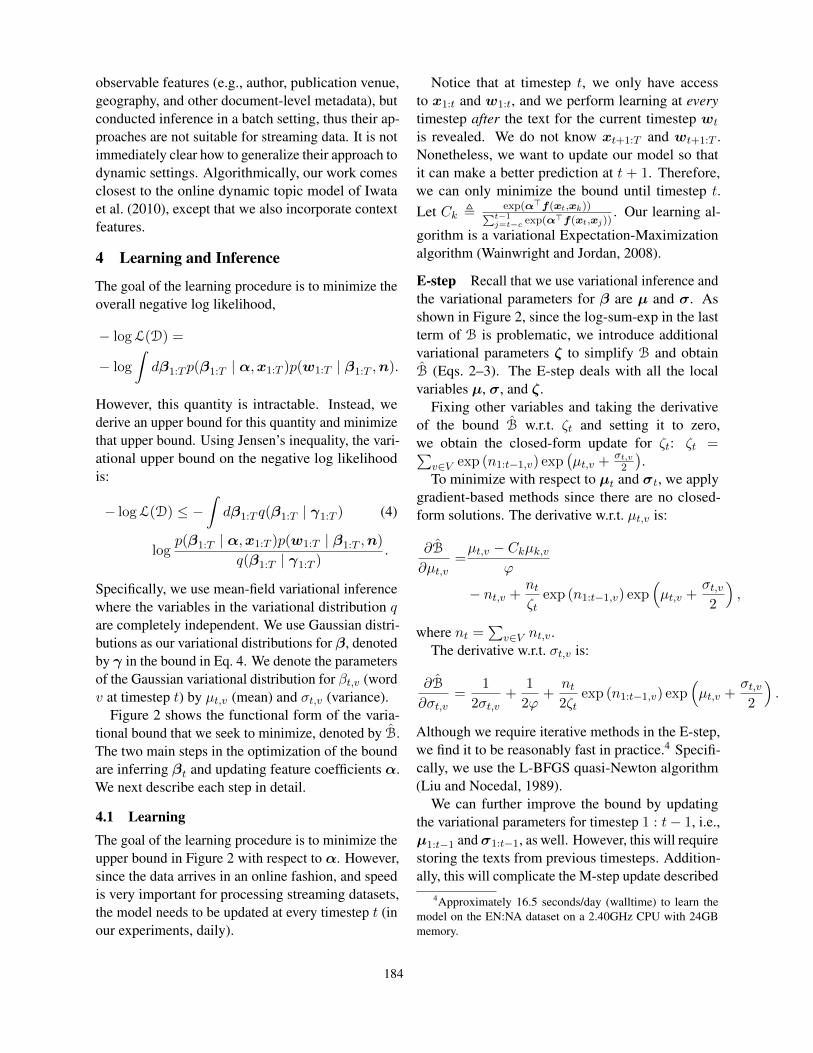
Figure 2 shows the functional form of the varia-tional bound that we seek to minimize, denoted by B.The two main steps in the optimization of the boundare inferring βt and updating feature coefficients α.We next describe each step in detail.

4.1 LearningThe goal of the learning procedure is to minimize theupper bound in Figure 2 with respect to α. However,since the data arrives in an online fashion, and speedis very important for processing streaming datasets,the model needs to be updated at every timestep t (inour experiments, daily).

Notice that at timestep t, we only have accessto x1:t and w1:t, and we perform learning at everytimestep after the text for the current timestep wt

is revealed. We do not know xt+1:T and wt+1:T .Nonetheless, we want to update our model so thatit can make a better prediction at t + 1. Therefore,we can only minimize the bound until timestep t.Let Ck , exp(α>f(xt,xk))Pt−1

j=t−c exp(α>f(xt,xj))

. Our learning al-

gorithm is a variational Expectation-Maximizationalgorithm (Wainwright and Jordan, 2008).

E-step Recall that we use variational inference andthe variational parameters for β are µ and σ. Asshown in Figure 2, since the log-sum-exp in the lastterm of B is problematic, we introduce additionalvariational parameters ζ to simplify B and obtainB (Eqs. 2–3). The E-step deals with all the localvariables µ, σ, and ζ.

Fixing other variables and taking the derivativeof the bound B w.r.t. ζt and setting it to zero,we obtain the closed-form update for ζt: ζt =∑

v∈V exp (n1:t−1,v) exp(µt,v +

σt,v2

).

To minimize with respect to µt and σt, we applygradient-based methods since there are no closed-form solutions. The derivative w.r.t. µt,v is:

∂B

∂µt,v=µt,v − Ckµk,v

ϕ

− nt,v +ntζt

exp (n1:t−1,v) exp(µt,v +

σt,v2

),

where nt =∑

v∈V nt,v.The derivative w.r.t. σt,v is:

∂B

∂σt,v=

1

2σt,v+

1

2ϕ+nt2ζt

exp (n1:t−1,v) exp(µt,v +

σt,v2

).

Although we require iterative methods in the E-step,we find it to be reasonably fast in practice.4 Specifi-cally, we use the L-BFGS quasi-Newton algorithm(Liu and Nocedal, 1989).

We can further improve the bound by updatingthe variational parameters for timestep 1 : t− 1, i.e.,µ1:t−1 andσ1:t−1, as well. However, this will requirestoring the texts from previous timesteps. Addition-ally, this will complicate the M-step update described

4Approximately 16.5 seconds/day (walltime) to learn themodel on the EN:NA dataset on a 2.40GHz CPU with 24GBmemory.

184

B =−T∑

t=1

Eq[log p(βt | βk,α,xt)]−T∑

t=1

Eq[log p(wt | βt,nt)]−H(q) (1)

=T∑

t=1

1

2

∑

j∈Vlog

σt,jϕ− Eq

−

(βt −

∑t−1k=t−c Ckβk

)2

2ϕ

− Eq

∑

v∈wt

n1:t−1,v + βt,v − log∑

j∈Vexp(n1:t−1,j + βt,j)

(2)

≤T∑

t=1

1

2

∑

j∈Vlog

σt,vϕ

+

(µt −

∑t−1k=t−c Ckµk

)2

2ϕ+σt +

∑t−1k=t−c C

2kσk

2ϕ

−∑

v∈wt

µt,v − log ζt −

1

ζt

∑

j∈Vexp (n1:t−1,j) exp

(µt,j +

σt,j2

)

+ const (3)

Figure 2: The variational bound that we seek to minimize, B. H(q) is the entropy of the variational distribution q. Thederivation from line 1 to line 2 is done by replacing the probability distributions p(βt | βk,α,xt) and p(wt | βt,nt)by their respective functional forms. Notice that in line 3 we compute the expectations under the variational distributionsand further bound B by introducing additional variational parameters ζ using Jensen’s inequality on the log-sum-exp inthe last term. We denote the new bound B.

below. Therefore, for each s < t, we choose to fixµs and σs once they are learned at timestep s.

M-step In the M-step, we update the global pa-rameter α, fixing µ1:t. Fixing other parameters andtaking the derivative of B w.r.t. α, we obtain:5

∂B

∂α=(µt −

∑t−1k=t−cCkµk)(−

∑t−1k=t−c

∂Ck∂α )

ϕ

+

∑t−1k=t−cCkσk

∂Ck∂α

ϕ,

where:

∂Ck∂α

=Ckf(xt,xk)

−Ck∑t−1

s=t−c f(xt,xs) exp(α>f(xt,xs))∑t−1

s=t−c exp(α>f(xt,xs))

.

We follow the convex optimization strategy and sim-ply perform a stochastic gradient update: αt+1 =

αt + ηt∂B∂αt

(Zinkevich, 2003). While the variationalbound B is not convex, given the local variables µ1:t

5In our implementation, we augment α with a squared L2

regularization term (i.e., we assume that α is drawn from anormal distribution with mean zero and variance λ) and use theFOBOS algorithm (Duchi and Singer, 2009). The derivativeof the regularization term is simple and is not shown here. Ofcourse, other regularizers (e.g., the L1-norm, which we use forother parameters, or the L1/∞-norm) can also be explored.

and σ1:t, optimizing α at timestep t without know-ing the future becomes a convex problem.6 Sincewe do not reestimate µ1:t−1 and σ1:t−1 in the E-step,the choice to perform online gradient descent insteadof iteratively performing batch optimization at everytimestep is theoretically justified.

Notice that our overall learning procedure is stillto minimize the variational upper bound B. All thesechoices are made to make the model suitable forlearning in real time from large streaming datasets.Preliminary experiments showed that performingmore than one EM iteration per day does not consid-erably improve performance, so in our experimentswe perform one EM iteration per day.

To learn the parameters of the model, we rely onapproximations and optimize an upper bound B. Wehave opted for this approach over alternatives (suchas MCMC methods) because of our interest in theonline, large-data setting. Our experiments show thatwe are still able to learn reasonable parameter esti-mates by optimizing B. Like online variational meth-ods for other latent-variable models such as LDA(Sato, 2001; Hoffman et al., 2013), open questions re-main about the tightness of such approximations andthe identifiability of model parameters. We note, how-

6As a result, our algorithm is Hannan consistent w.r.t. thebest fixed α (for B) in hindsight; i.e., the average regret goes tozero as T goes to∞.

185

ever, that our model does not include latent mixturesof topics and may be generally easier to estimate.

5 Prediction

As described in §2.2, our model is evaluated by theloss suffered at every timestep, where the loss isdefined as the negative log likelihood of the modelon text at timestep wt. Therefore, at each timestep t,we need to predict (the distribution of)wt. In orderto do this, for each word v ∈ V , we simply computethe deviation means βt,v as weighted combinationsof previous means, where the weights are determinedby the world-context similarity encoded in x:

Eq[βt,v | µt,v] =t−1∑

k=t−c

exp(α>f(xt,xk))∑t−1j=t−c exp(α

>f(xt,xj))µk,v.

Recall that the word distribution that we use forprediction is obtained by applying the operator πthat maps βt and n to the V -dimensional simplex,forming a distribution over words: π(βt,n1:t−1)v =

exp(n1:t−1,v+βt,v)Pj∈V exp(n1:t−1,j+βt,j)

, where n1:t−1,v ∈ RV is abackground distribution (the log-frequency of wordv observed up to time t− 1).

6 Experiments

In our experiments, we consider the problem of pre-dicting economy-related text appearing in news andmicroblogs, based on observable features that reflectcurrent economic conditions in the world at a giventime. In the following, we describe our dataset in de-tail, then show experimental results on text prediction.In all experiments, we set the window size c = 7 (oneweek) or c = 14 (two weeks), λ = 1

2|V | (V is thesize of vocabulary of the dataset under consideration),and ϕ = 1.

6.1 DatasetOur data contains metadata and text corpora. Themetadata is used as our features, whereas the textcorpora are used for learning language models andpredictions. The dataset (excluding Twitter) canbe downloaded at http://www.ark.cs.cmu.edu/DynamicLM.

6.1.1 MetadataWe use end-of-day stock prices gathered from

finance.yahoo.com for each stock included in

the Standard & Poor’s 500 index (S&P 500). Theindex includes large (by market value) companieslisted on US stock exchanges.7 We calculate daily(continuously compounded) returns for each stock, o:ro,t = logPo,t− logPo,t−1, where Po,t is the closingstock price.8 We make a simplifying assumption thattext for day t is generated after Po,t is observed.9

In general, stocks trade Monday to Friday (exceptfor federal holidays and natural disasters). For dayswhen stocks do not trade, we set ro,t = 0 for allstocks since any price change is not observed.

We transform returns into similarity values as fol-lows: f(xo,t, xo,k) = 1 iff sign(ro,t) = sign(ro,k)and 0 otherwise. While this limits the model by ig-noring the magnitude of price changes, it is still rea-sonable to capture the similarity between two days.10

There are 500 stocks in the S&P 500, so xt ∈ R500

and f(xt,xk) ∈ R500.

6.1.2 Text dataWe have five streams of text data. The first four

corpora are news streams tracked through Reuters.11

Two of them are written in English, North AmericanBusiness Report (EN:NA) and Japanese InvestmentNews (EN:JP). The remaining two are German Eco-nomic News Service (DE, in German) and FrenchEconomic News Service (FR, in French). For all fourof the Reuters streams, we collected news data overa period of thirteen months (392 days), 2012-05-26to 2013-06-21. See Table 1 for descriptive statisticsof these datasets. Numerical terms are mapped to asingle word, and all letters are downcased.

The last text stream comes from the Deca-hose/Gardenhose stream from Twitter. We collectedpublic tweets that contain ticker symbols (i.e., sym-bols that are used to denote stocks of a particularcompany in a stock market), preceded by the dollar

7For a list of companies listed in the S&P 500 as of2012, see http://en.wikipedia.org/wiki/List_of_S\%26P_500_companies. This set was fixed duringthe time periods of all our experiments.

8We use the “adjusted close” on Yahoo that includes interimdividend cash flows and also adjusts for “splits” (changes in thenumber of outstanding shares).

9This is done in order to avoid having to deal with hourlytimesteps. In addition, intraday price data is only availablethrough commercial data provided.

10Note that daily stock returns are equally likely to be positiveor negative and display little serial correlation.

11http://www.reuters.com

186

Dataset Total # Doc. Avg. # Doc. #Days Unigrams BigramsTotal # Tokens Size Vocab. Total # Tokens Size Vocab.

EN:NA 86,683 223 392 28,265,550 10,000 11,804,201 5,000EN:JP 70.807 182 392 16,026,380 10,000 7,047,095 5,000

FR 62,355 160 392 11,942,271 10,000 3,773,517 5,000DE 51,515 132 392 9,027,823 10,000 3,499,965 5,000

Twitter 214,794 336 639 1,660,874 10,000 551,768 5,000

Table 1: Statistics about the datasets. Average number of documents (third column) is per day.

sign $ (e.g., $GOOG, $MSFT, $AAPL, etc.). Thesetags are generally used to indicate tweets about thestock market. We look at tweets from the period2011-01-01 to 2012-09-30 (639 days). As a result,we have approximately 100–800 tweets per day. Wetokenized the tweets using the CMU ARK TweetNLPtools,12 numerical terms are mapped to a single word,and all letters are downcased.

We perform two experiments using unigram andbigram language models as the base models. Foreach dataset, we consider the top 10,000 unigramsafter removing corpus-specific stopwords (the top100 words with highest frequencies). For the bigramexperiments, we only use 5,000 words to limit thenumber of unique bigrams so that we can simulateexperiments for the entire time horizon in a reason-able amount of time. In standard open-vocabularylanguage modeling experiments, the treatment of un-known words deserves care. We have opted for acontrolled, closed-vocabulary experiment, since stan-dard smoothing techniques will almost surely interactwith temporal dynamics and context in interestingways that are out of scope in the present work.

6.2 Baselines

Since this is a forecasting task, at each timestep, weonly have access to data from previous timesteps.Our model assumes that all words in all documentsin a corpus come from a single multinomial distri-bution. Therefore, we compare our approach to thecorresponding base models (standard unigram and bi-gram language models) over the same vocabulary (foreach stream). The first one maintains counts of everyword and updates the counts at each timestep. Thiscorresponds to a base model that uses all of the avail-able data up to the current timestep (“base all”). Thesecond one replaces counts of every word with the

12https://www.ark.cs.cmu.edu/TweetNLP

counts from the previous timestep (“base one”). Ad-ditionally, we also compare with a base model whosecounts decay exponentially (“base exp”). That is, thecounts from previous timesteps decay by exp(−γs),where s is the distance between previous timestepsand the current timestep and γ is the decay constant.We set the decay constant γ = 1. We put a symmetricDirichlet prior on the counts (“add-one” smoothing);this is analogous to our treatment of the backgroundfrequencies n in our model. Note that our model,similar to “base all,” uses all available data up totimestep t− 1 when making predictions for timestept. The window size c only determines which previ-ous timesteps’ models can be chosen for making aprediction today. The past models themselves are es-timated from all available data up to their respectivetimesteps.

We also compare with two strong baselines: a lin-ear interpolation of “base one” models for the pastweek (“int. week”) and a linear interpolation of “baseall” and “base one” (“int one all”). The interpolationweights are learned online using the normalized expo-nentiated gradient algorithm (Kivinen and Warmuth,1997), which has been shown to enjoy a strongerregret guarantee compared to standard online gra-dient descent for learning a convex combination ofweights.

6.3 Results

We evaluate the perplexity on unseen dataset to eval-uate the performance of our model. Specifically, weuse per-word predictive perplexity:

perplexity = exp

(−∑T

t=1 log p(wt | α,x1:t,n1:t−1)∑Tt=1

∑j∈V wt,j

).

Note that the denominator is the number of tokensup to timestep T . Lower perplexity is better.

Table 2 and Table 3 show the perplexity results for

187

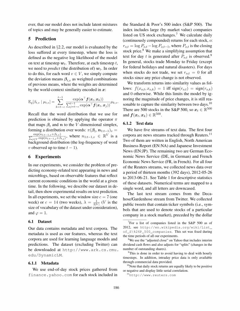
Dataset base all base one base exp int. week int. one all c = 7 c = 14

EN:NA 3,341 3,677 3,486 3,403 3,271 3,262 3,285EN:JP 2,802 3,212 2,750 2,949 2,708 2,656 2,689

FR 3,603 3,910 3,678 3,625 3,416 3,404 3,438DE 3,789 4,199 3,979 3,926 3,634 3,649 3,687

Twitter 3,880 6,168 5,133 5,859 4,047 3,801 3,819

Table 2: Perplexity results for our five data streams in the unigram experiments. The base models in “base all,” “baseone,” and “base exp” are unigram language models. “int. week” is a linear interpolation of “base one” from the pastweek. “int. one all” is a linear interpolation of “base one” and “base all”. The rightmost two columns are versions ofour model. Best results are highlighted in bold.

Dataset base all base one base exp int. week int. one all c = 7

EN:NA 242 2,229 1,880 2,200 244 223EN:JP 185 2,101 1,726 2,050 189 167

FR 159 2,084 1,707 2,068 166 139DE 268 2,634 2,267 2,644 282 243

Twitter 756 4,245 4,253 5,859 4,046 739

Table 3: Perplexity results for our five data streams in the bigram experiments. The base models in “base all,” “baseone,” and “base exp” are bigram language models. “int. week” is a linear interpolation of “base one” from the pastweek. “int. one all” is a linear interpolation of “base one” and “base all”. The rightmost column is a version of ourmodel with c = 7. Best results are highlighted in bold.

each of the datasets for unigram and bigram experi-ments respectively. Our model outperformed othercompeting models in all cases but one. Recall that weonly define the similarity function of world contextas: f(xo,t, xo,k) = 1 iff sign(ro,t) = sign(ro,k) and0 otherwise. A better similarity function (e.g., onethat takes into account market size of the companyand the magnitude of increase or decrease in the stockprice) might be able to improve the performance fur-ther. We leave this for future work. Furthermore,the variations can be captured using models from thepast week. We discuss why increasing c from 7 to 14did not improve performance of the model in moredetail in §6.4.

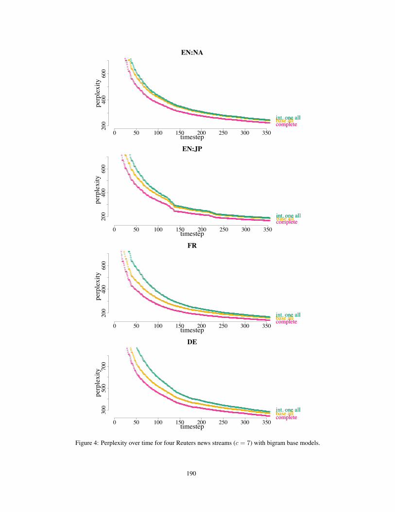
We can also see how the models performed overtime. Figure 4 traces perplexity for four Reuters newsstream datasets.13 We can see that in some cases theperformance of the “base all” model degraded overtime, whereas our model is more robust to temporal

13In both experiments, in order to manage the time and spacecomplexities of updating β, we apply a sparsity shrinkage tech-nique by using OWL-QN (Andrew and Gao, 2007) when maxi-mizing it, with regularization constant set to 1. Intuitively, thisis equivalent to encouraging the deviation vector to be sparse(Eisenstein et al., 2011).

shifts.In the bigram experiments, we only ran our model

with c = 7, since we need to maintain β in RV 2,

instead of RV in the unigram model. The goal ofthis experiment is to determine whether our methodstill adds benefit to more expressive language mod-els. Note that the weights of the linear interpolationmodels are also learned in an online fashion sincethere are no classical training, development, and testsets in our setting. Since the “base one” model per-formed poorly in this experiment, the performance ofthe interpolated models also suffered. For example,the “int. one all” model needed time to learn that the“base one” model has to be downweighted (we startedwith all interpolated models having uniform weights),so it was not able to outperform even the “base all”model.

6.4 Analysis and DiscussionIt should not be surprising that conditioning onworld-context reduces perplexity (Cover and Thomas,1991). A key attraction of our model, we believe, liesin the ability to inspect its parameters.

Deviation coefficients. Inspecting the model al-lows us to gain insight into temporal trends. We

188

Twitter:Google

timestep

β

0 100 200 300 400 500 600

0.00.51.01.52.0

googgoog

@google@googlegoogle+google+

#goog#goog

rGOOGrGOOG

Twitter:Microsoft

timestep

β

0 100 200 300 400 500 600

0.0

0.5

1.0

1.5

microsoftmicrosoft

msftmsft#microsoft#microsoft

rMSFTrMSFT

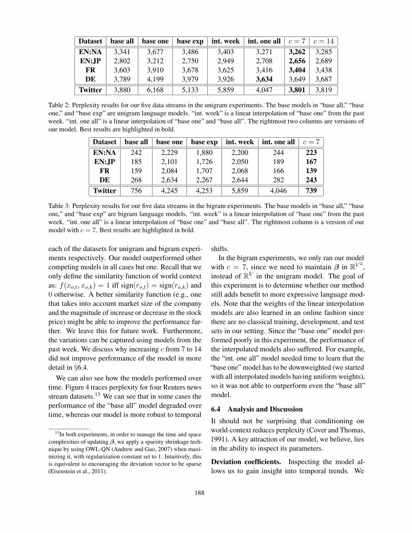
Figure 3: Deviation coefficients β over time for Google- and Microsoft-related words on Twitter with unigram basemodel (c = 7). Significant changes (increases or decreases) in the returns of Google and Microsoft stocks are usuallyfollowed by increases in β of related words.

investigate the deviations learned by our model on theTwitter dataset. Examples are shown in Figure 3. Theleft plot shows β for four words related to Google:goog, #goog, @google, google+. For compari-son, we also show the return of Google stock for thecorresponding timestep (scaled by 50 and centered at0.5 for readability, smoothed using loess (Cleveland,1979), denoted by rGOOG in the plot). We can seethat significant changes of return of Google stocks(e.g., the rGOOG spikes between timesteps 50–100,150–200, 490–550 in the plot) occurred alongsidean increase in β of Google-related words. Similartrends can also be observed for Microsoft-relatedwords in the right plot. The most significant loss ofreturn of Microsoft stocks (the downward spike neartimestep 500 in the plot) is followed by a suddensharp increase in β of the words #microsoft andmicrosoft.

Feature coefficients. We can also inspect thelearned feature coefficients α to investigate whichstocks have higher associations with the text thatis generated. Our feature coefficients are designedto reflect which changes (or lack of changes) instock prices influence the word distribution more,not which stocks are talked about more often. Wefind that the feature coefficients do not correlate withobvious company characteristics like market capi-talization (firm size). For example, on the Twitterdataset with bigram base models, the five stocks withthe highest weights are: ConAgra Foods Inc., IntelCorp., Bristol-Myers Squibb, Frontier Communica-tions Corp., and Amazon.com Inc. Strongly negativeweights tended to align with streams with less activ-

time lags

frequency

020

4060

80

1 2 3 4 5 6 7 8 9 10 11 12 13 14

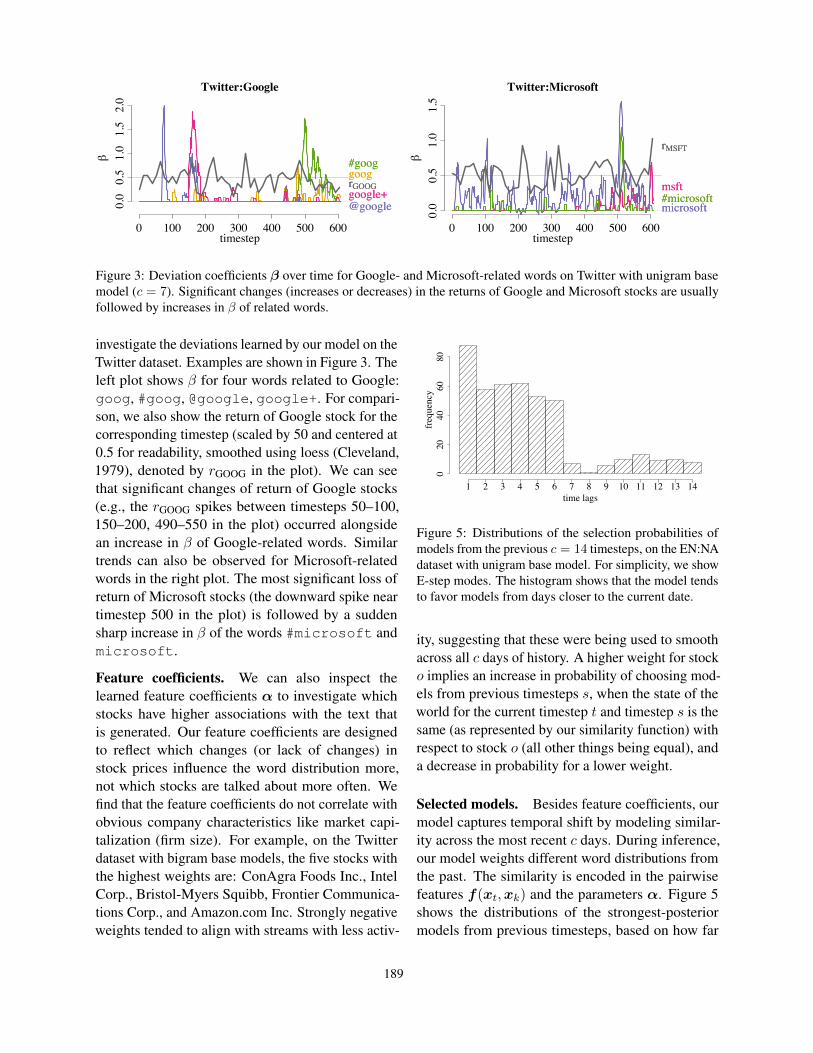
Figure 5: Distributions of the selection probabilities ofmodels from the previous c = 14 timesteps, on the EN:NAdataset with unigram base model. For simplicity, we showE-step modes. The histogram shows that the model tendsto favor models from days closer to the current date.

ity, suggesting that these were being used to smoothacross all c days of history. A higher weight for stocko implies an increase in probability of choosing mod-els from previous timesteps s, when the state of theworld for the current timestep t and timestep s is thesame (as represented by our similarity function) withrespect to stock o (all other things being equal), anda decrease in probability for a lower weight.

Selected models. Besides feature coefficients, ourmodel captures temporal shift by modeling similar-ity across the most recent c days. During inference,our model weights different word distributions fromthe past. The similarity is encoded in the pairwisefeatures f(xt,xk) and the parameters α. Figure 5shows the distributions of the strongest-posteriormodels from previous timesteps, based on how far

189

EN:NA

timestep

perplexity

0 50 100 150 200 250 300 350

200

400

600

base allbase allcompletecompleteint. one allint. one all

EN:JP

timestep

perplexity

0 50 100 150 200 250 300 350

200

400

600

base allbase allcompletecompleteint. one allint. one all

FR

timestep

perplexity

0 50 100 150 200 250 300 350

200

400

600

base allbase allcompletecompleteint. one allint. one all

DE

timestep

perplexity

0 50 100 150 200 250 300 350

300

500

700

base allbase allcompletecompleteint. one allint. one all

Figure 4: Perplexity over time for four Reuters news streams (c = 7) with bigram base models.

190

in the past they are at the time of use, aggregatedacross rounds on the EN:NA dataset, for window sizec = 14. It shows that the model tends to favor modelsfrom days closer to the current date, with the t − 1models selected the most, perhaps because the stateof the world today is more similar to dates closer totoday compare to more distant dates. The plot alsoexplains why increasing c from 7 to 14 did not im-prove performance of the model, since most of thevariation in our datasets can be captured with modelsfrom the past week.

Topics. Latent topic variables have often figuredheavily in approaches to dynamic language model-ing. In preliminary experiments incorporating single-membership topic variables (i.e., each document be-longs to a single topic, as in a mixture of unigrams),we saw no benefit to perplexity. Incorporating top-ics also increases computational cost, since we mustmaintain and estimate one language model per topic,per timestep. It is straightforward to design mod-els that incorporate topics with single- or mixed-membership as in LDA (Blei et al., 2003), an in-teresting future direction.

Potential applications. Dynamic language modelslike ours can be potentially useful in many applica-tions, either as a standalone language model, e.g.,predictive text input, whose performance may de-pend on the temporal dimension; or as a componentin applications like machine translation or speechrecognition. Additionally, the model can be seen asa step towards enhancing text understanding withnumerical, contextual data.

7 Conclusion

We presented a dynamic language model for stream-ing datasets that allows conditioning on observablereal-world context variables, exemplified in our ex-periments by stock market data. We showed how toperform learning and inference in an online fashionfor this model. Our experiments showed the predic-tive benefit of such conditioning and online learningby comparing to similar models that ignore temporaldimensions and observable variables that influencethe text.

AcknowledgementsThe authors thank several anonymous reviewers for help-ful feedback on earlier drafts of this paper and BrendanO’Connor for help with collecting Twitter data. This re-search was supported in part by Google, by computingresources at the Pittsburgh Supercomputing Center, byNational Science Foundation grant IIS-1111142, AFOSRgrant FA95501010247, ONR grant N000140910758, andby the Intelligence Advanced Research Projects Activ-ity via Department of Interior National Business Centercontract number D12PC00347. The U.S. Government isauthorized to reproduce and distribute reprints for Govern-mental purposes notwithstanding any copyright annotationthereon. The views and conclusions contained herein arethose of the authors and should not be interpreted as nec-essarily representing the official policies or endorsements,either expressed or implied, of IARPA, DoI/NBC, or theU.S. Government.

ReferencesGalen Andrew and Jianfeng Gao. 2007. Scalable training

of l1-regularized log-linear models. In Proc. of ICML.David M. Blei and John D. Lafferty. 2006. Dynamic topic

models. In Proc. of ICML.David M. Blei, Andrew Y. Ng, and Michael I. Jordan.

2003. Latent Dirichlet allocation. Journal of MachineLearning Research, 3:993–1022.

Sebastien Bubeck. 2011. Introduction to online opti-mization. Technical report, Department of OperationsResearch and Financial Engineering, Princeton Univer-sity.

Nicolo Cesa-Bianchi and Gabor Lugosi. 2006. Prediction,Learning, and Games. Cambridge University Press.

William S. Cleveland. 1979. Robust locally weightedregression and smoothing scatterplots. Journal of theAmerican Statistical Association, 74(368):829–836.

Thomas M. Cover and Joy A. Thomas. 1991. Elements ofInformation Theory. John Wiley & Sons.

John Duchi and Yoram Singer. 2009. Efficient onlineand batch learning using forward backward splitting.Journal of Machine Learning Research, 10(7):2899–2934.

Jacob Eisenstein, Brendan O’Connor, Noah A. Smith,and Eric P. Xing. 2010. A latent variable model forgeographic lexical variation. In Proc. of EMNLP.

Jacob Eisenstein, Amr Ahmed, and Eric P. Xing. 2011.Sparse additive generative models of text. In Proc. ofICML.

Amit Goyal, Hal Daume III, and Suresh Venkatasubrama-nian. 2009. Streaming for large scale NLP: Languagemodeling. In Proc. of HLT-NAACL.

191

Matt Hoffman, David M. Blei, Chong Wang, and JohnPaisley. 2013. Stochastic variational inference. Jour-nal of Machine Learning Research, 14:1303–1347.

Antti Honkela and Harri Valpola. 2003. On-line varia-tional Bayesian learning. In Proc. of ICA.

Tomoharu Iwata, Takeshi Yamada, Yasushi Sakurai, andNaonori Ueda. 2010. Online multiscale dynamic topicmodels. In Proc. of KDD.

Frederick Jelinek. 1997. Statistical Methods for SpeechRecognition. MIT Press.

Jyrki Kivinen and Manfred K. Warmuth. 1997. Expo-nentiated gradient versus gradient descent for linearpredictors. Information and Computation, 132:1–63.

Victor Lavrenko, Matt Schmill, Dawn Lawrie, PaulOgilvie, David Jensen, and James Allan. 2000. Miningof concurrent text and time series. In Proc. of KDDWorkshop on Text Mining.

Abby Levenberg and Miles Osborne. 2009. Stream-basedrandomised language models for SMT. In Proc. ofEMNLP.

Abby Levenberg, Chris Callison-Burch, and Miles Os-borne. 2010. Stream-based translation models for sta-tistical machine translation. In Proc. of HLT-NAACL.

Dong C. Liu and Jorge Nocedal. 1989. On the limitedmemory BFGS method for large scale optimization.Mathematical Programming B, 45(3):503–528.

David Mimno and Andrew McCallum. 2008. Topic mod-els conditioned on arbitrary features with Dirichlet-multinomial regression. In Proc. of UAI.

Alexander Rakhlin. 2009. Lecture notes on online learn-ing. Technical report, Department of Statistics, TheWharton School, University of Pennsylvania.

Masaaki Sato. 2001. Online model selection based on thevariational bayes. Neural Computation, 13(7):1649–1681.

Shai Shalev-Shwartz. 2012. Online learning and onlineconvex optimization. Foundations and Trends in Ma-chine Learning, 4(2):107–194.

Martin J. Wainwright and Michael I. Jordan. 2008. Graph-ical models, exponential families, and variational infer-ence. Foundations and Trends in Machine Learning,1(1–2):1–305.

Chong Wang, David M. Blei, and David Heckerman.2008. Continuous time dynamic topic models. In Proc.of UAI.

Chong Wang, John Paisley, and David M. Blei. 2011. On-line variational inference for the hierarchical Dirichletprocess. In Proc. of AISTATS.

Martin Zinkevich. 2003. Online convex programmingand generalized infinitesimal gradient ascent. In Proc.of ICML.

192