dynamic interactions of life and its landscape: … · dynamic interactions of life and its...

EARTH SURFACE PROCESSES AND LANDFORMSEarth Surf. Process. Landforms 35, 78–101 (2010)Copyright © 2010 John Wiley & Sons, Ltd.Published online in Wiley InterScience(www.interscience.wiley.com) DOI: 10.1002/esp.1912

State of Science

Dynamic interactions of life and its landscape: feedbacks at the interface of geomorphology and ecologyLiam Reinhardt1*, Douglas Jerolmack2, Brad J. Cardinale3, Veerle Vanacker4 and Justin Wright5

1 University of Exeter.2 University of Pennsylvania.3 University of California, Santa Barbara.4 University of Louvain.5 Duke University

Received 13 May 2009; 7 August 2009; 17 August 2009

*Correspondence to: L. Reinhardt, University of Exeter, full address. Email: [email protected]

ABSTRACT: There appears to be no single axis of causality between life and its landscape, but rather, each exerts a simultane-ous infl uence on the other over a wide range of temporal and spatial scales. These infl uences occur through feedbacks of differing strength and importance with co-evolution representing the tightest coupling between biological and geomorphological systems. The ongoing failure to incorporate these dynamic bio-physical interactions with human activity in landscape studies limits our ability to predict the response of landscapes to human disturbance and climate change. This limitation is a direct result of the poor communication between the ecological and geomorphological communities and consequent paucity of interdisciplinary research. Recognition of this failure led to the organization of the Meeting of Young Researchers in Earth Science (MYRES) III, titled ‘Dynamic Interactions of Life and its Landscape’. This paper synthesizes and expands upon key issues and fi ndings from that meeting, to help chart a course for future collaboration among Earth surface scientists and ecologists: it represents the con-sensus view of a competitively selected group of 77 early-career researchers. Two broad themes that serve to focus and motivate future research are identifi ed: (1) co-evolution of landforms and biological communities; and (2) humans as modifi ers of the landscape (through direct and indirect actions). Also outlined are the state of the art in analytical, experimental and modelling techniques in ecological and geomorphological research, and novel new research avenues that combine these techniques are suggested. It is hoped that this paper will serve as an interdisciplinary reference for geomorphologists and ecologists looking to learn more about the other fi eld. Copyright © 2010 John Wiley & Sons, Ltd.

Introduction

The predominant view in many fi elds of natural science has long been that biology is an epiphenomenon of the physical environment. A cursory look at textbooks in biology, geology, chemistry, and others reveals the vast number of para-digms that are founded on the idea that the abundance, biomass, and distribution of organisms on the planet is dependent upon spatial and temporal variation in physical processes, which con-strain where life can exist and how much life can exist. This view has been prominent for many decades despite an earlier recogni-tion within the natural sciences that life and its landscape are intimately related through ‘interactions between the organic and inorganic’ (Darwin, 1881; Tansley, 1935). Although feedbacks were not forgotten entirely, they received much less attention during the 20th century than many alternative topics, perhaps because increasing specialization and disciplinary boundaries minimized interactions among biologists and physical scientists (Renschler et al., 2007; Corenblit et al., 2008). However, in

recent decades researchers have returned to early views about bio-physical interactions, and have begun to show in detail how organisms not only respond to their physical environment, but also directly modify and control their physical environment in ways that promote their own persistence. Entire bodies of research such as biogeomorphology (Viles, 1988), ‘ecological stoichiom-etry’ (Sterner and Elser, 2002), ‘ecosystem engineering’ (Jones et al., 1994), and ‘biodiversity and ecosystem functioning’ (Loreau et al., 2002) have emerged to illustrate how the numbers and types of plants and animals that inhabit an ecosystem can directly control the fl uxes of energy and matter that underlie biogeo-chemical cycles, gas fl uxes, sediment transport, and the forma-tion of new physical habitat. Complimentary developments in the fi eld of ‘ecohydrology’ have also revealed numerous ways in which plants and animals can alter water fl ow paths and soil moisture/depth to the advantage of those species (McCarthy et al., 1998; Rodriguez-Iturbe and Porporato, 2004; Yoo et al., 2005b; D’Odorico and Porporato, 2006; Tamea, 2007; Muneepeerakul et al., 2008a, 2008b)

DYNAMIC INTERACTIONS OF LIFE AND ITS LANDSCAPE 79

Copyright © 2010 John Wiley & Sons, Ltd. Earth Surf. Process. Landforms, Vol. 35, 78–101 (2010)DOI: 10.1002/esp

If physical processes drive ecosystem structure, while the evolving structure also modulates physical processes, then feedbacks between the two are likely to be important. However, not all bio-physical interactions will have a signifi -cant effect upon landscape functioning and an extreme end-member exists where life is absent from a landscape; deciding whether and where bio-physical feedbacks are important is a key challenge. Abiotic landscapes must have existed on Earth prior to the colonization of land by plants during the Silurian and they are currently observed on Mars (Dietrich and Perron, 2006; Corenblit and Steiger, 2009). The Earths terrestrial land-scape has undergone considerable modifi cation since the Silurian in conjunction with the evolution of terrestrial life; the degree to which physical landscapes may co-evolve with bio-logical systems is discussed in detail in this paper.

It has proven diffi cult to incorporate bio-physical feedbacks into existing (numerical, physical and conceptual) models in part because their importance depends upon the temporal (and likely spatial) scale under consideration (Schumm and Lichty, 1965), and more importantly because such feedbacks are likely to give rise to emergent behaviour that prevents the use of simple ‘linearly additive’ models (Werner, 2003). Yet the need to make society-relevant predictions has never been more important. Climate models are now entering an era where regional projections for temperature and rainfall changes are possible (IPCC, 2007). Unfortunately, our models for landscape evolution are not yet at this stage. What we need is to develop a new set of conceptual as well as mathematical models of life–landscape coupling that can account for emer-gent behaviour; fundamental science must be done to eluci-date bio-physical coupling across a range of scales. To advance this goal and to promote interdisciplinary research efforts by ecologists and geomorphologists a group of early career scientists from around the world met at the third Meeting of Young Researchers in Earth Science (MYRES III) at Tulane University in 2008: discussion revolved around the theme ‘Dynamic Interactions of Life and its Landscape’. During the course of 4 days of discussion, 77 competitively-selected international delegates explored several key areas for future research: can one demonstrate a defi nite signature of life in landscape form? how does the functional diversity of organisms infl uence and feed back on landscape change? and do the structures of landscapes and ecosystems co-evolve? In the following sections we expand upon these themes by iden-tifying: (a) the state of the art; (b) knowledge gaps; and (c) ways forward in the study of bio-physical interactions. We also suggest two areas in which advancements in basic science will have immediate and important practical consequence: advancing the application and success of landscape restora-tion techniques, and predicting landscape susceptibility to destabilization from climate change.

During the MYRES workshop we also discussed some of the analytical, experimental and modelling techniques that are now available to ecologists and geomorphologists. It was sur-prising how little each of us knew of techniques and methods in other disciplines. In order that we may encourage interdis-ciplinary research, and to some degree explain what is pos-sible, we begin this paper by outlining some of the most powerful analytical, experimental and modelling techniques in ecological and geomorphological research, and suggest novel research avenues that may combine these approaches.

New Techniques and Methods

Recent decades have seen the development of a wealth of new techniques and technologies in both ecology and geomor-

phology. There are enormous benefi ts to be gained in integrat-ing these ‘tools’ to answer some of society’s most pressing issues. We present here an overview of some of the most powerful and/or most underutilized techniques of which we are aware. Numerical and physical modelling are discussed in separate sub-sections due the scope and complexity of these topics. We hope that this overview and attendant bibli-ography will serve as a useful starting point for future interdis-ciplinary research.

Analytical tools for the fi eld and laboratory

State of artPerhaps the most pervasive and most underutilized ‘toolbox’ currently available to ecologists and geomorphologists is that of remote sensing. Remote sensing is a term which encom-passes both the science behind image acquisition hardware and the subsequent processing of data supplied by those systems. A broad suite of systems and techniques are avail-able, including:

• ground-based, close range proximal sensing instruments such as hyperspectral spectroradiometers (Milton et al., in press) and high defi nition laser scanners (Wehr, 2008);

• airborne multispectral scanners, multispectral video systems, thermal imaging sensors, aerial photography, light detection and ranging (LiDAR) sensors (Lefsky et al., 2002), and side-looking airborne RADAR;

• spaceborne satellite systems, including nadir-viewing mul-tispectral sensors, interferometric synthetic aperture RADAR (InSAR) systems, and multiple view angle systems capable of capturing anisotropic signatures (Diner et al., 1998).

The repeat survey capabilities of new multi- and hyper-spectral remotely sensed systems and missions can now be employed towards the assessment of landscape change over a range of spatial and temporal scales. The Landsat series of satellites (Landsat 1 launched in 1972) can now provide up to 36 years of repeat-visit multi-spectral global coverage (Goward et al., 2001; Williams et al., 2006; Gillanders et al., 2008) and this long time series has benefi ted studies of vegetation change and ecological modelling (Cohen and Goward, 2004). Further developments in the Landsat mission are planned with the Landsat Data Continuity Mission (LDCM), due for launch in 2012 (Irons and Masek, 2006; Wulder et al., 2008). Active systems such as RADAR and LiDAR produce their own electro-magnetic radiation, offering near-all-weather capabilities. These systems are primarily used for monitoring structure – either of the land surface or of the overlying vegetation (Rabus et al., 2003; Parker et al., 2004; Watt and Donoghue, 2005; Su and Bork, 2007; Moorthy et al., 2008; Straatsma et al., 2008).

More recently, the NASA Earth Observing System (EOS) has provided repeat-visit products from which physical landscape properties and dynamics may be obtained (Katra and Lancaster, 2008; Rowan and Mars, 2003). New opportunities for fi ne-scale observations are now possible, from a new generation of satellite sensors such as IKONOS (Hurtt et al., 2003), Quickbird (Clark et al., 2004; Wang et al., 2004) and SPOT-5 (Pasqualini et al., 2005) which have multispectral pixel resolu-tions of 10 m or less. On the ground, fi eld-based spectroradi-ometers offer even fi ner spectral and spatial resolution data (Anderson and Kuhn, 2008). When combined with local and regional observations of water and sediment yields, such observations can be used to relate bio-physical process interactions over a wide range of temporal and spatial

80 L. REINHARDT ET AL.


scales (Hilker et al., 2008; Chen et al., 2009; Connolly et al., 2009).

Alongside the development of remote sensing techniques has been a concomitant revolution in fi eld and laboratory techniques. A suite of stable and radioactive isotopes now allow dating of sediment and bedrock ages (and erosion rates) over a wide range of temporal scales. Short lived isotopes such as 210Pb, 241Am and 137Cs enable dating of buried sediment over the past ∼150 years (Appleby and Oldfi eld, 1978, 1992; He and Walling, 1996), with new high-resolution techniques allowing the near-annual dating of deposits from individual fl oods (Aalto et al., 2003; 2008), plus independent determina-tion of surface exposure time for sediments on fl oodplain surfaces. New advances also allow the measurement of extremely low 14C concentrations, enabling the dating of organic material up to 60 kyrs old (Bird et al., 1999; Turney et al., 2001, 2006). Radioactive cosmogenic nuclides (10Be and 26Al, 36Cl) can determine the age of sedimentary deposits up to 5 Myrs old (Granger and Muzikar, 2001), while stable nuclides such as 3He and 21Ne can be used to date multi-million year old bedrock surfaces (Schafer et al., 1999). Optically stimulated luminescence provides an independent (non-radiometric) technique for measuring the age of buried sediment over the same age range as 14C, and in rare instances >105 years (Huntley et al., 1985; Jain et al., 2004). Another extraordinary technique allows us to estimate the upstream erosion rate of an entire river catchment from a single river sediment sample: 10Be concentrations in river-borne quartz integrate erosion rates over >102 years (Brown et al., 1995; Bierman and Steig, 1996; Granger et al., 1996). These new techniques have allowed us to quantify transience and persis-tence in erosional and depositional records in all terrestrial environments. For instance, it has been shown that the Antarctic dry valleys have remained essentially unchanged for several million years, due most likely to the almost complete absence of water – and, by extension, ‘life’ (Summerfi eld et al., 1999). Conversely, extremely rapid rates of erosion and sediment compaction (<26 mm year−1) have been measured in high mountains and deltaic environments, respectively (Schaller et al., 2005; Reinhardt et al., 2007; Tornqvist et al., 2008). Rates of human disturbance of physical processes have also been quantifi ed, e.g. 137Cs carbon inventory measure-ments (Van Oost et al., 2007).

Knowledge gapsThere appears to be enormous untapped potential in the vast amounts of data currently available to researchers. Remote sensing tools, particularly satellite based systems, generate data at a pace that outstrips the average user’s ability to utilize it fully. These ‘tools’ offer adequate spatial resolution of the Earths surface but observing bio-physical interactions typically requires a higher temporal resolution than is cur-rently available. We need to be able to observe feedbacks such as those between landslides and vegetation colonization in steep mountain terrain, and the response and recovery of landscapes to forest fi re. In addition, we have few tools for measuring subsurface heterogeneities and biological activity and none of them provide the type of global cover that is now routinely available through remote sensing. This is a critical knowledge gap as a large proportion of ecological activity and biogeochemical cycling occurs in the subsurface; groundwa-ter fl ow is also a key parameter in hydrological models.

A more general knowledge gap lies in the relatively short record of measured landscape dynamics (<102 years). Many biological processes operate over decadal or shorter times-cales (with peat development being an obvious exception) and

are therefore amenable to direct measurement. Unfortunately, physical processes operating over much longer time period are diffi cult or impossible to measure directly. Perhaps more importantly we have thus far been unable to quantify the timescale of bio-physical interactions in most situations: one of the classic examples is precipitation recycling through evapotranspiration, which could infl uence landform develop-ment over millennia (Worden et al., 2007). In this context it is crucial that we use reliable palaeo-landscape proxies to quantify landscape dynamics.

Ways forwardPalaeo-community dynamics are now accessible through a variety of proxies (e.g. plant macrofossils (Birks and Birks, 2000), testate amoeba – bog water tables – (Charman, 2001), pollen (Heikki and Bennett, 2003), and stable isotopes (Melanie et al., 2004)). Of particular note is recent work by the PolLandCal group which may enable the spatial distribution of palaeo-plant communities to be reconstructed from fossil pollen (Gaillard et al., 2008). Progress is also beginning to be made in integrating palaeo-ecology with landuse/land cover records (Dearing et al., 2008). The pace of progress can be accelerated if the suite of cutting edge analytical technologies in both ecology and geomorphology are integrated. Remotely sensed imagery, numerous isotopic proxies, biomarkers and genetic analyses now allow determination of the physical and ecological structure of modern landscapes. To our knowledge, no study to date has combined the best of these approaches.

New isotopic proxies for physical and biological processes and new methods for analyzing high-resolution data sets are emerging all the time. Biological organisms fractionate iso-topes such as carbon, oxygen and sulfur, while physical pro-cesses may fractionate calcium and strontium (for example), providing a parallel set of stable isotopes. Combining such proxies would allow unprecedented reconstructions of the chemical conditions of the past. If coupled with traditional stratigraphic analysis, plus modern analogue studies of where and how isotopes are fractionated, biogeochemical methods would allow us to extend the record of bio-physical interac-tions into deep geologic time.

Aside from the technical advances in the use of isotopes and remote sensing there are many new statistical methods that may help integrate ecology and geomorphology. We argue in this paper that there is no single axis of causality between life and its landscape, but rather, that each exerts a simultaneous infl uence on the other. This perspective requires that we move away from univariate models of causality that assume a single independent and dependent variable, and move towards models that assume two or more processes are operating simultaneously – in other words, we must have methods to evaluate more complex, multivariate relationships where estimates must be made for numerous pathways at once. This is where statistical tools such as structural equa-tions modelling (SEM) (Shipley, 2000; Grace, 2006), Bayesian hierarchical modelling (Gelman and Hill, 2007) and related methodologies are opening up new opportunities (Clark, 2007). These methods allow for the direct testing of hypoth-eses that are conditioned on more than one causal pathway. For example, SEM fi ts data from an observed covariance matrix among variables to a matrix that would be expected based on the hypothetical set of relationships among the causal and response variables. As such, these models allow one to test for simultaneous causality among two or more variables, to estimate indirect effects among variables, and to directly incorporate spatial or temporal feedbacks into a hypothesis.



Development and validation of landscape evolution models that enable feedbacks between biological and physical processes

State of the artTo date, biological effects have been incorporated into four general types of geomorphic transport law (GTL) used to model: transport rates, thresholds of motion, slope stability, and hydraulic roughness (cf Dietrich et al., 2003). In most of these numerical formulations biotic effects implicitly control the value of a parameter, such as thresholds for slope stability and fl uvial incision, rather than acting as an explicit dynamic variable that interacts with geomorphic processes (see review by Dietrich and Perron, 2006). Initial steps in advancing GTLs for bio-physical interactions have included the development of equations that explicitly incorporate the dynamics of animal population (Yoo et al., 2005b) and root density to soil depth (Roering, 2008). Other recent develop-ments include GTLs that relate landslide initiation to forest growth and death (Benda and Dunne, 1997; Lancaster et al., 2003), or human-induced land use change (Vanacker et al., 2003b) and solve simple dynamic equations describing vege-tation-erosion interactions over storm and inter-storm times-cales forced by random rain events (Figure 1) (Tucker and Bras, 1999; Collins et al., 2004; Istanbulluoglu and Bras, 2005). Climatic and ecohydrological controls however have not been fully incorporated in these models (for simulations of large-scale basins) over geomorphically signifi cant times-

cales. Some recent analytical models of ecohydrological soil moisture, water balance, and vegetation dynamics that share the same simplistic view/spirit with the existing GTLs offer tremendous opportunities in this context (Rodriguez-Iturbe and Porporato, 2004). In the simplest sense, these interactions may be distilled into time-space integrated variables for long-term and large-scale landscape evolution modelling such as in the forms postulated below:

Q = KA Ssm n (1)

and

K f p B t k B t B dtc

A

= ( ) ( )( ) ( ){ }∫ , , , ,λ τ (2)

where K is an integrated sediment transport coeffi cient, A is upslope contributing area, S is local landscape slope, and m and n are exponents that characterize the form of geomorphic transport (e.g. m = 0 for creep and m > 1 for wash). Equation (1) determines the transport rate (Qs) of sediment at any point on the landscape as a function of local topography and fl ow conditions (Howard and Kerby, 1983; Tucker and Whipple, 2002). In Equation (2), K is postulated to be an integrated coeffi cient that takes into account biomass as a dynamic state variable. In K, p is mean storm intensity; λ is storm arrival rate; B is vegetation biomass; τc is erosion threshold as a function of vegetation biomass, k is transport coeffi cient or erodibility that depends on both substrate size and plant biomass, and t

Figure 1. Numerical simulations illustrating the contrasting difference in landscape morphology under conditions of constant uniform uplift and (A) no vegetation cover, (B) static uniform vegetation cover, (C) dynamic vegetation. All landscapes are in dynamic equilibrium, with mean eleva-tions subject to fl uctuations about a long-term mean. In the absence of vegetation (A) rainstorms generate frequent erosion events forming a highly dissected, low-relief topography. In the contrasting case (B), static (undying) vegetation protects the soil surface from runoff erosion. Continuing uplift under this condition increases the elevations until slopes exceed the critical threshold for landsliding and hillslope erosion is predominantly by mass wasting. In the third case (C) of dynamic vegetation, disturbances are driven by runoff erosion and landslides. Compared with the static vegetation simulation the outcome of vegetation-erosion coupling is a more highly dissected topography, with smaller landslide-dominated hollows entering the channel network; mean elevation is approximately three times smaller than that of the static vegetation simulation. The effect of wildfi res on landscape development is explored in other simulations presented in this work (Istanbulluoglu and Bras, 2005).



is time. A numerical example of this model was given by Istanbulluoglu and Bras (2006), who used a bucket model of hydrology to examine the infl uence of climate fl uctuations/change on potential sediment transport capacity. While such forms may be adequate for characterizing long-term and reach-scale average transport and incision rates, they may not capture sudden impacts of climate change and two-way inter-actions of vegetation and erosion.

Knowledge gapsSubsuming biotic effects within existing GTLs is probably adequate in certain, as yet undefi ned, situations but our view is that in general more dynamic transport laws need to be incorporated into models. Plant biomass (both above and below ground), and some measures to quantify vegetation cover density, seasonality and the morophological diversity of plant structures (for example, differences in rooting structure), are necessary ecological variables for modelling the infl uence of vegetation on erosion and sediment transport. A recent paper by Montaldo et al. (2005) discusses vegetation models with various complexities that involve some of the aforemen-tioned vegetation variables, and develops ways to simplify models as needed. In addition, numerical and physical model-ling suggest that the destructive impact of erosion and/or deposition on an ecosystem (or disturbance as used in ecology literature) is just as important as the impact of vegetation on sediment transport mechanisms (see review by Murray et al., 2008). Quantitative research into the impact of physical pro-cesses upon ecosystems has largely been confi ned to the ecological literature, although geomorphologists have begun to develop functional forms that relate vegetation loss to erosion and/or deposition and sediment transport for use in numerical models (Gyssels et al., 2005). Most functional rela-tions developed to date are lab based and upscaling to the landscape scale is problematic. In the existing literature the disruptive effect of erosion to the ecosystem is accomplished by rule-based approximations (Istanbulluoglu and Bras, 2005; Baas and Nield, 2007).

Determining appropriate temporal and spatial scales is usually a challenge in numerical modelling. Erosion rates and landscape patterns are known to exhibit a dependence on grid resolution in landscape evolution models (Passalacqua et al., 2006). Choosing appropriate grid spacing requires some knowledge of the time and space scales associated with the processes we are trying to model. For example, in a model for river channel evolution, conservation of mass implies a ‘mor-phodynamic’ timescale while the numerical grid must be fi ne enough to resolve important features of the channel. Determination of the most relevant time and space scales for bio-physical interactions is critical to model success, as inap-propriate selection may preclude feedbacks from arising. That requires, however, that these scales are a priori known, which is often not the case.

Ways forwardWe view the development of verifi able predictive life–landscape models to be a key challenge. This new class of models needs to be simple enough to run over long-timescales, capture some of the most necessary aspects of climate–soil–vegetation–animal interactions, and have spa-tially explicit functions that allow competition between differ-ent vegetation functional types and species in space and time. The most relevant bio-physical processes responsible for shaping the landscape should be identifi ed and included in the developing models. We stress the importance of nonlinear local interactions between animals, vegetation and physical processes through mechanisms such as grazing, seed dispersal,

and competition for soil moisture and light. Inclusion of these interactions will enable study of emergent patterns of landscapes.

1. There is momentum within the geomorphic modelling community towards integration of (or at least communica-tion between) the wide variety of extant landscape evolu-tion models. One of the most important initiatives in this regard is the Community Surface Dynamics Modelling System (CSDMS), which makes a host of numerical models available to the community (www.csdms.colorado.edu). CSDMS has begun to encourage their modelling commu-nity to integrate formulations for dynamic bio-physical interactions within their hosted models (G. Tucker. pers commun.). Another promising type of model, which has successfully been employed in ecology in recent decades, is agent or actor based numerical modelling (Judson, 1994). Such models employ a number of decision making entities that generally execute autonomy, communication/interac-tion and decision making (Parker et al., 2004), and appear capable of accommodating the complex interplay between humans and animals and their environment. This class of model is discussed in more detail later.

2. Developing new models that explicitly integrate biological and physical processes over the timescales of plant and human life or shorter is critical for modelling the human impact on the physical and the biological environment. Ecosystem dynamics operate at much shorter timescales than long-term GTLs, which are often calibrated over 1000-year timescales. The way forward is either to nest models requiring short timescales within longer-term surface process models, or alternatively, by examining separately the short-term transient dynamics of a system relative to the longer-term equilibrium dynamics (Hastings, 2004).

3. Determination of the timescales of physical and biological processes is key to understanding when, and how, they will interact. This also provides one potential path forward in dealing with issues of scale. For example, in considering whether vegetation dynamics interact with channel evolu-tion in a river, one could determine both the characteristic timescale of vegetation growth and the characteristic ‘mor-phodynamic’ timescale of the river. In considering how the channel and vegetation interact, the absolute values of these two timescales are not important: rather, it is the ratio of these timescales that determines the nature of their interaction.

4. Statistical parameterization of smaller-scale processes may be required before we can generate large-scale mathemati-cal models of heterogeneous systems. These techniques are already well established in the geophysics community: groundwater modellers use geostatistical methods to deal with permeability variations, and Large Eddy Simulation (LES) models parameterize the small-scale fl uctuations of fl uid turbulence in a statistical manner. Perhaps these sta-tistical parameterizations can be used to model heteroge-neity in rates of biological growth, chemical reactions and transport in large-scale landscape simulations. The LES approach has shown promise in resolving the grid-depen-dent issues of numerical landscape evolution models (Passalacqua et al., 2006)

5. Simplifi ed models for describing bio-physical feedbacks should be developed in parallel with more sophisticated landscape evolution models. While the ultimate goal of numerical modelling may be quantitative prediction, such predictive power is a long way off as many constitutive and dynamic relationships among variables have yet to be worked out (Fonstad, 2006; Phillips, 2006). Identifying



potential (nonlinear) feedbacks between physical and biological processes is necessary to make progress. In complex pattern-forming systems such as landscapes, the strong coupling among processes often dictates that system dynamics must be better represented than the details of individual processes (Murray, 2007; Murray et al., 2008). Models that allow for a ‘rules based’ approach, like cellular automata (Fonstad, 2006), can serve to integrate mechanics and intuition in order to test ideas of life–landscape cou-pling. These models may be qualitatively and even semi-quantitatively predictive, but most importantly they can serve to generate hypotheses about the forms of physical and biological coupling in landscapes.

6. Model outputs must be compared in some way with inde-pendent data to be of scientifi c value. True verifi cation of landscape evolution models is unlikely but validation in the sense that a model ‘does not contain known or detect-able fl aws and is internally consistent’ is achievable (Oreskes et al., 1994, p.642). Comparison of mathematical models with physical models may be benefi cial in this regard as both methods are capable of independently pro-ducing the same result (i.e. a model landscape); direct comparison between independent models should also advance our understanding of bio-physical interactions. Current model tests are generally ambiguous and overly focused on weak topographic metrics. The modelling com-munity needs to agree upon a suite of spatial and tempo-rally sensitive tests of model output (Hoey et al., 2003). These tests should allow for a hierarchal scale of model ‘validations’ of differing strength. Inclusion of ecological dynamics, which operate on relatively short timescales, may provide new temporally-sensitive tests.

Physical modelling: motivating and constraining bio-physical experiments

State of the artThe use of experiments to physically model Earth surface processes has a long august history in geomorphology (Gilbert, 1914). Until recently the most effective experiments were prototype systems that were dynamically scaled down from fi eld scales using dimensionless ratios. The strength of this approach is that if all relevant ratios are matched between experiment and prototype then measurements made in an experiment can be scaled up to the fi eld (Paola et al., 2009). However, models involving free fl owing water (i.e. most surface process models) cannot be perfectly scaled to a labora-tory size as no available fl uid has a kinematic viscosity signifi -cantly less than water. Despite this limitation engineers have routinely shown that so long as the small-scale water fl ow is fully turbulent in both prototype and fi eld then water can be used in prototype models (this is termed Reynolds-number independence in the literature).

It has recently been argued that formal scaling is unneces-sary for a subset of landscapes that exhibit scale independence in their important processes. ‘By scale independence we mean that the important dynamics of a system are independent of scale over a signifi cant scale range’ (Paola et al., 2009, p.34). Scale independent systems would be unaffected by changes in scale and thus make natural targets for experimental study at reduced scale ‘without recourse to classical dynamical scaling’ (Paola et al., 2009). If this new paradigm is correct it means that we can look forward to a rapid advance in our understanding of geomorphic systems within a sub-set of natural environments (Paola et al., 2009): to-date this sub-set is thought to include high-relief mountains, braided channels

and large depositional systems (Lague et al., 2003; Kim and Paola, 2007).

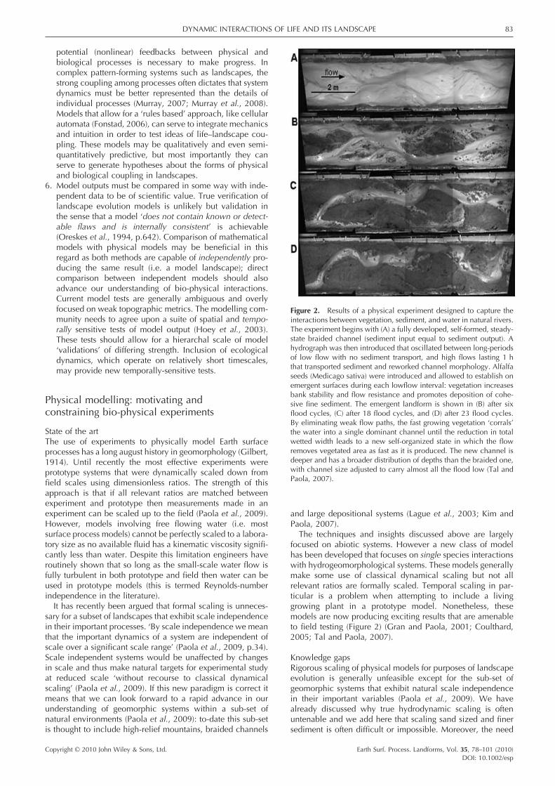
The techniques and insights discussed above are largely focused on abiotic systems. However a new class of model has been developed that focuses on single species interactions with hydrogeomorphological systems. These models generally make some use of classical dynamical scaling but not all relevant ratios are formally scaled. Temporal scaling in par-ticular is a problem when attempting to include a living growing plant in a prototype model. Nonetheless, these models are now producing exciting results that are amenable to fi eld testing (Figure 2) (Gran and Paola, 2001; Coulthard, 2005; Tal and Paola, 2007).

Knowledge gapsRigorous scaling of physical models for purposes of landscape evolution is generally unfeasible except for the sub-set of geomorphic systems that exhibit natural scale independence in their important variables (Paola et al., 2009). We have already discussed why true hydrodynamic scaling is often untenable and we add here that scaling sand sized and fi ner sediment is often diffi cult or impossible. Moreover, the need

Figure 2. Results of a physical experiment designed to capture the interactions between vegetation, sediment, and water in natural rivers. The experiment begins with (A) a fully developed, self-formed, steady-state braided channel (sediment input equal to sediment output). A hydrograph was then introduced that oscillated between long-periods of low fl ow with no sediment transport, and high fl ows lasting 1 h that transported sediment and reworked channel morphology. Alfalfa seeds (Medicago sativa) were introduced and allowed to establish on emergent surfaces during each lowfl ow interval: vegetation increases bank stability and fl ow resistance and promotes deposition of cohe-sive fi ne sediment. The emergent landform is shown in (B) after six fl ood cycles, (C) after 18 fl ood cycles, and (D) after 23 fl ood cycles. By eliminating weak fl ow paths, the fast growing vegetation ‘corrals’ the water into a single dominant channel until the reduction in total wetted width leads to a new self-organized state in which the fl ow removes vegetated area as fast as it is produced. The new channel is deeper and has a broader distribution of depths than the braided one, with channel size adjusted to carry almost all the fl ood low (Tal and Paola, 2007).



for compressing time as well as space means that materials that erode or weather slowly in the fi eld – like bedrock – cannot be scaled directly for laboratory experiments. In addi-tion, rheologic and material properties of sediment mixtures may not be amenable to downscaling. A notorious example is the diffi culty of creating meandering rivers in the laboratory, which is likely related to issues of downscaling sediment cohesion. For modelling bio-physical interactions, biota such as vegetation may well introduce fundamental length and timescales (related to the size and growth rate of plants, respectively) that cannot be reproduced in a laboratory. Conversely, some bio-physical interactions might include scale independence in their important variables as implied by some of the more successful experiments undertaken to date (e.g. Tal and Paola, 2007). This issue remains unresolved as we await the development of more robust theoretical basis for prototyping bio-physical interactions.

Ways forwardThe use of classically dynamically scaled prototypes will con-tinue to be an important investigative method. However, natural similarity seems to provide a far more fl exible and expansive framework for experimental design and interpreta-tion. It is not yet known how ‘widespread natural scale inde-pendence is in morphodynamics, but the evidence to date suggests it is common’ (Paola et al., 2009, p.37). We will not know until researchers investigate this further, and compari-son of bio-physical dynamics across scales is an obvious way to tackle this. Identifying the rates and timescales of important physical and biological processes, and how they compete to generate landforms is also of primary importance. We hypoth-esize that it is the relative – rather than absolute – timescales of competing processes that dictate pattern formation and evolution in simple bio-physical systems, and that correctly identifying and scaling them leads to dynamic similarity. For example, Jerolmack and Mohrig (2007) demonstrated that the relative magnitude of channel bank erosion and bed deposi-tion timescales controls channel pattern, allowing direct com-parison between fi eld and laboratory observations.

It is unlikely that we will ever be able to dynamically scale ecological-community interactions in a small prototype. In a forthcoming section we discuss why ecosystem dynamics might be important to landscape functioning so here we confi ne ourselves to the practical issues involved in develop-ing effective models. Modelling the interactions of many dif-ferent species on an evolving landscape is not easy, because each organism introduced has its own length and timescales of growth. In addition, simplifying the experimental system requires neglecting variables. If very little is known about the nature of bio-physical feedbacks in a natural landscape, an oversimplifi ed model may be constructed that precludes important feedbacks from developing. Field work has its own drawbacks, because the confounding effects of environmental variability make it diffi cult to separate cause and effect. Fortunately the development of fi eld-scale experiments offers a way forward. There are now a small number of fi eld-scale experiments that enable study of multi-species (ecological community) interactions with abiotic processes. One example is the ‘Outdoor Stream Lab’ at St. Anthony Falls Laboratory, Minnesota. This is a reach-scale system designed to study interactions among channel, fl oodplain and vegetation (www.safl .umn.edu/facilities/OSL.html). Another example is at the University of Arizona’s Biosphere 2, where several large experimental hillslopes are under construction (http://www.b2science.org/Earth-hillslope.html). This setup will allow the study of vegetation growth and its infl uence on hydrology, biogeochemical fl uxes and sediment transport, through exten-

sive monitoring under carefully controlled conditions for approximately 10 years.

Co-evolution of Landforms and Biological Communities

Within the fi eld of biology, the term ‘co-evolution’ was coined to describe the simultaneous adaptation by populations inter-acting so closely that each exerts a strong selective force on the other (Ehrlich and Raven 1964). Co-evolution is a classic example of a feedback in which genetic, and subsequently, morphological change by one population induces change in a second population that, in turn, feeds back to stimulate further adaptation by the fi rst. Although co-evolution is typi-cally used to describe biological interactions and implies the action of natural selection, there are a number of conceptual parallels to bio-physical feedbacks whereby physical pro-cesses constrain the selective environment that drives biologi-cal evolution while the biotic community simultaneously modifi es the physical environment at a variety of spatial and temporal scales (Urban and Daniels, 2006; Renschler et al., 2007; Corenblit et al., 2008). For purposes of this paper, we defi ne such bio-physical forms of co-evolution as: ‘feedbacks in which the physical environment regulates the numbers and types of organisms that can coexist in a community and shape the selective environment that drives evolution while, at the same time, the organisms themselves modify the environment in a way that enhances their own persistence.’ This defi nition does not imply that biological communities evolve as a group or whole. Indeed, the idea of community-level evolution (also called group selection) has been highly controversial; many argue there is no clear mechanism that can drive the evolution of groups that do not share common genes (Wilson, 1983). However, any collection of species or populations can share common life-history characteristics (growth rates, resource requirements, etc.) that cause them to respond to, or modify a landscape in a manner that is similar to one another. Furthermore, certain types of biological interactions like facili-tation can cause the success of two populations to be mutually dependent. Thus, it is plausible for groups of organisms that comprise biological communities to simultaneously cause and respond to a changing landform.

State of the artThere is a long and rich history of research in biology showing that changing landforms can cause changes in the abundance, biomass, numbers, and types of species that co-occur in any particular geographic location at a point in time. For example, the most widely cited mechanism to explain the formation of new life-forms is the process of allopatric speciation, which occurs when the formation of a geographic barrier (e.g. moun-tain range, canyon, or river) isolates two populations allowing them to genetically diverge from one another through time (Coyne and Orr, 2004). Paleobiologists and biogeographers have also shown that once species diverge, the distribution and survival probability of a new species is heavily infl uenced by geological processes, such as the movement of tectonic plates (Raven and Axelrod, 1974), volcanism (Miller, 1997), and the advance and retreat of glaciers (Hewitt, 1996). Even at smaller spatial scales, the fi eld of ecology has shown that the assembly of ecological communities is strongly controlled by the frequency of disturbances (fl oods, hurricanes, land-slides, etc.) that regenerate physical habitats and open up new niche opportunities that allow species to use untapped resources (Connell, 1979; Huston, 1979). Indeed, one could likely pick up any introductory textbook in these fi elds of



biology and fi nd dozens, if not hundreds, of examples where the organization of biological communities is presumed to be the outcome of physical processes that drive the formation of landscapes.

As discussed in the introduction to this paper the converse idea that biological communities act as an independent vari-able to drive the formation of landscapes is certainly not a new concept. For example, in his seminal book Vernadsky (1929) argued that life fundamentally shaped climate, atmo-sphere, and landforms. However, the role of biology in con-trolling rates of physical processes was not a prominent focus of ecological research until the 1990s when accelerating rates of species extinction forced researchers to pose the ques-tion . . . What do species do in ecosystems (Jones and Lawton, 1995)? One of the concepts to emerge during this period was that of ecosystem engineering (Figure 3), in which species tend to physically modify and/or create habitat in ways that can potentially enhance their own survival and/or the existence of other species (Figure 4).

Historical examples abound of organisms having large-scale effects on geomorphology and landscape formation. For example, Ives (1942) suggested that the valley fl oor elevation and ‘false senility’ of stream networks (i.e. extensive meanders and ox-bow lakes in relatively young stream networks) throughout the Rocky Mountains was due to the activity of beaver; subsequent research has supported this view (Naiman et al., 1988; Gurnell, 1998). Mima mounds – Earth mounds approximately 20–30 m in diameter and as much as 2 m high, found throughout the western two-thirds of North America and other grassland habitats, have been hypothesized to have been created through soil translocation by fossorial rodents (Dalquest and Sheffer, 1942; Cox, 1984). Butler (1995) com-piled an extensive list of examples of what he termed ‘zoogeo-morphology’ or animals as geomorphic agents ranging from invertebrates to large mammals. The concept of organisms as ecosystem engineers has organized these scattered examples of organisms modifying the environment into a more general framework and has begun to make signifi cant progress towards some unifying themes (Wright and Jones, 2006). Of particular importance are attempts to understand how variation in the spatial and temporal scale of ecosystem engineering affect the feedbacks to the ecosystem engineer and the consequences to the landscape (Gilad et al., 2004; Jones et al., 1997; Wright and Jones, 2006; Van Hulzen et al., 2007). These examples of ecosystem engineering demonstrate that biological agents can alter the formation of landscapes. In many cases, the modifi cation of landscapes by organisms would seem to be ‘accidental’, i.e. to offer little fi tness advantage to the organ-isms themselves (what Odling-Smee et al., (2003) called ‘neg-ative niche construction’, or ‘niche changing’ sensu Dawkins (2004)). However, in other cases there are clear examples where modifi cation of the landscape directly benefi ts the species. Such situations have been termed an ‘extended phe-notype’ (Dawkins, 1999) or ‘niche construction’ (Laland et al., 1999; Odling-Smee, 2003), and suggest that biology and land-scape formation can feed back to simultaneously infl uence one another. Unfortunately, quantifying these types of feed-backs and showing they operate qualitatively in space or time lags far behind the speculation.

Perhaps the most advanced research in the area of co-evolution of landforms and biological communities stems from studies that have examined how biota both respond to and control sediment transport processes. Van Hulzen et al. (2007) described how Spartina anglica (common cordgrass) both modifi es its habitat via its own physical structures, and then responds to those modifi cations. Spartina tends to enhance the accretion of sediments within the plant canopy

Ecosystemengineer

Structuralchange

Abioticchange

Bioticchange

+

+ Engineer,predator,prey,competitor,etc.

Ecosystem engineering process

Ecosystem engineering consequence

Positive or negative effects on other organisms and on the engineer+

Figure 3. General pathways of physical ecosystem engineering (Gutierrez and Jones, 2008).

0 8 17 25 33 42

1

0.75

0.50

0.25

060 65 70 75 80 85

Velocity (cm sec -1)

Str

eam

bed

stab

ility

(pro

port

ion

of s

tabl

e pa

rtic

les)

Increase in velocity (%)

2542m -2

904m -2

0 larvae m -2

Figure 4. The fi eld of ‘ecosystem engineering’ suggests that organ-isms directly create or modify habitat in ways that enhance their own persistence. As just one example, consider the results of Cardinale et al. (2004) who used a laboratory fl ume study to show that the con-struction of catchnets by net-spinning caddisfl y larvae can increase the physical stability of substrates in streams. The more larvae (densi-ties shown on right side), the more stable were substrates relative to control that had no organisms. Data points are the mean +/− SE from three replicate fl umes.



by reducing hydrodynamic energy and scour. Sediment accre-tion feeds back positively to enhance Spartina densities by increasing drainage and nutrient availability. But as sediment accretion leads to increased Spartina densities, gullies that form around the tussocks of plant growth inhibit the lateral expansion of Spartina through cloning of roots. In other words, the plant modifi es the environment so that it becomes more locally favourable, but these modifi cations alter the process of erosion that create small ‘islands’ and inhibit spread of the plant. Other authors have shown how vegetation-driven sedi-ment accretion enables vegetated surfaces to persist even under rates of sea level rise and sediment delivery that would normally preclude intertidal surfaces (and vegetation) from developing in the fi rst place (Kirwan and Murray, 2007; Marani et al., 2007). As a second example, it has long been known that the biomass, as well as composition and diversity of riparian plant communities along streams and rivers is controlled by fl ow regimes that infl uence the physical stability of bank habitats (reviewed in Naiman and Decamps 1997). However, recent laboratory experiments by Tal and Paola (2007) have shown that vegetation can also act as an inde-pendent variable to stabilize streambanks in ways that ‘corral’ the water and control the formation and stability of a channel. Thus, vegetation not only responds to channel formation and stability, it also directly infl uences it.

Modelling studies have also explored the two-way interplay between vegetation growth/succession and sediment transport in aeolian sand dunes (Baas and Nield, 2007), estuarine (Morris et al., 2002; Mudd et al., 2004; D’Alpaos et al., 2007; Kirwan and Murray, 2007; Temmerman et al., 2007) and fl uvial systems (Lancaster and Baas, 1998; Maun and Perumal, 1999; Collins et al., 2004; Istanbulluoglu and Bras, 2005). Researchers have also begun to explore feedbacks between macrofauna, vegetation, soil formation and sediment trans-port. Burrowing animals and plants disturb soil and enhance soil ‘creep’ thereby regulating soil thickness and hillslope form, providing a feedback mechanism whereby soil develop-ment limits the species that inhabit it (Yair, 1995; Gabet et al., 2003; Yoo et al., 2005a, 2005b; Meysman et al., 2006; Roering, 2008; Phillips, 2009).

Knowledge gapsAlthough several case studies have begun to detail co-evolu-tion between biological communities and landscape forma-tion, we have little understanding of how feedbacks between biology and physics actually work. We have a comparatively decent understanding of how physical processes drive biology but our understanding of how biology infl uences physical processes is confi ned to a scattering of case studies that lack a clearly organized conceptual framework. As a result, we have little idea of the spatial and temporal scales at which biology might shift from a cause to a consequence of physical processes (cf Schumm and Lichty, 1965) and little idea of how to go about detecting such shifts. There are many examples where biology exhibits a clear effect on physical processes at a small scale, including the binding of river banks and bed substrate by vegetation and biomats (respectively); the bur-rowing effect of worms, gophers and fallen trees that loosens soil and enhances transport; corals and mangroves dissipating wave energy; vegetation infl uencing runoff and infi ltration; and biogeochemistry causing fl occulation of clay particles. It is not clear what the net effect of these processes is at signifi -cantly larger time and space scales.

Ways forwardIn this section we suggest ways in which we can advance our knowledge of co-evolution by asking three questions: (1) Is

there a topographic signature of life and, if so, at what scale(s) is this signature apparent? (2) Is it possible to ‘demonstrate co-evolution of life and its landscape?’ (3) To what extent does biodiversity infl uence the evolution of landscapes?

Is there a topographic signature of life and, if so, at what scale(s) is this signature apparent?

The fi rst step towards generating an organizing framework is to ask is there a ‘fi ngerprint’ of biology on the landscape and, if so, at what scales do patterns that are specifi cally biogenic in origin manifest themselves? Clear examples of life signa-tures can be seen in large carbonate systems such as reefs and atolls and in smaller transitional landscapes such as parabolic dunes (Baas and Nield, 2007). It has even been suggested that the existence of granite is indirectly a result of life, through recycling of organic matter into the mantle during subduction (Lee et al., 2008). However, Dietrich and Perron (2006) argued that the overwhelming majority of landforms on Earth, while clearly modulated in their rate of evolution by biological processes, are not clearly biogenic in their origin. They posited that geological processes control biological processes over large spatial scale, whereas biological processes can in turn modify physical processes at much smaller ‘local’ scales. To the extent this is correct we should be able to detect scale-dependent signatures of life in the statistics of landscape topography. This is exactly what Lashermes et al. (2007) and Roering (in prep) found in their examination of 1 m resolution LiDAR elevation data from the Oregon Coast Range. The landscape appeared to be fractal across a wide range of scales (as is common), however, there was clear evidence of a scaling break below 7 m. This scale corresponds to the size of pit and mound features created from fallen trees. Statistical analysis of high resolution topographic data may reveal such scaling breaks in other landscapes. If fi eld work indicates that these breaks are related to known biogenic processes, we will have made a signifi cant conceptual step forward in demon-strating the relevance of biology to landscape form and func-tion, and to quantifying the scales at which these imprints occur. From a numerical modelling perspective, such scale-dependent processes indicate the scale at which coupling between physical and biological processes should be stron-gest. Direct process modelling of tree growth, tree throw, sediment movement and slope evolution could be carried out at the individual tree scale, and its macroscopic effect on hillslope evolution assessed by time-iterating a spatially extended model, for example.

Another place to search for a signature of life in landscapes is to resolve the temporal evolution of a landscape. While temporal dynamics are more diffi cult to resolve in slowly evolving landscapes than are spatial patterns, some progress may be made using modelling results as a guide. Recent mathematical modelling of landscape evolution indicates that the presence of vegetation results in more intermittent sedi-ment fl ux from a drainage basin and leads to steeper hillslope gradients (Istanbulluoglu and Bras, 2005). Analysis of land-scape morphology at least partly corroborates these model results, (Tucker et al., 2006; Istanbulluoglu et al., 2008).

Can we demonstrate co-evolution of life and its landscape?

We have proposed that the dynamics of life and its landscape are intertwined through a set of feedbacks of differing strength and importance, with co-evolution representing the tightest



coupling between biological and geomorphological systems. Co-evolution may potentially be demonstrated through a com-bined fi eld and model-testing approach that aims to recon-struct the paleo-dynamics of life and landscape interactions. A fi rst start would be to empirically determine how common co-evolved systems are, which would include attempting to resolve dynamics through reconstructing the trajectory of a landform and its ecological community through time, and using auto-regressive time series models to assess whether there is evidence for temporal feedbacks and dynamic cou-pling (Ives et al., 2003). In addition, some systems may be amenable to fi eld-scale experimental approaches.

At this early stage of investigation, we believe that the gen-eration of new hypotheses is of key importance. We suggest that simple exploratory models, founded on phenomenology and minimal representation rather than reductionism, be used to investigate life–landscape co-evolution (cf Fonstad, 2006). This challenge is distinct from the development of more sophisticated numerical models discussed earlier. We see application of simple models as leading to ‘frontier’ research that will guide more sophisticated investigations in the future. Simple models can direct us towards the types of data we need to collect and experiments to be undertaken in order to test hypotheses.

We may be able to isolate the infl uence a single species has on a landscape by studying fi eld areas affected by natural extinction or invasion events. Many ecosystems experience rapid loss of the numerically or biomass dominant species due to natural death, disease, or disturbance. Field or remote observations of such events (Ramsey et al., 2005; Pengra et al., 2007) will enable examination of how the loss and replace-ment of dominant species leads to changes in geomorphologi-cal processes. Similarly, invasive species displace native fl ora and/or fauna, and may have a concomitant effect, and feed-back, upon surface processes. Measurement of these interac-tions may be used to quantify the coupling between life and landscape, and may even offer opportunities to explore how the variety of life infl uences landscape formation.

To what extent does biodiversity infl uence the evolution of landscapes?

Earlier we mentioned that laboratory research on bio-physical interactions has, to date, focused on the impacts that indi-vidual plant species have on physical processes; similar research on single animal species has been conducted in the fi eld (Gabet et al., 2003; Yoo et al., 2005b; Katija and Dabiri, 2009). Clearly, however, species in nature are seldom found as monocultures. Even some of the least diverse ecosystems on Earth contain dozens, if not hundreds of interacting species. The question we raise here is does this biological variation matter? Can the effects of ‘life’ on physical processes be rea-sonably condensed into a single parameter that can be used to modify models of physical processes, or do we gain a qualitatively different understanding of natural phenomena by considering the great variation in life that exists on Earth? This is by no means a trivial question. It might be a relatively easy step to modify our understanding about geomorphic processes to consider the role that ‘plants’ play in physics. It would be quite another thing to consider the differing roles that grasses play as opposed to shrubs or trees, and another thing still to consider the roles played by dozens of individual species of grasses, shrubs, or trees (much less the genetic diversity within species populations).

One of the central tenets of ecology is that every species must somehow use biologically limiting resources in a ways that are spatially or temporally unique in order to coexist in nature (Chesson, 2000; Chase and Leibold, 2003). When this is the case, each species should, in theory, have a unique ‘niche’ that imparts a signature on its physical environment. It has been shown that diverse ecological communities com-posed of many species often produce more biomass per unit area (Figure 5) (Hector et al., 1999; Tilman et al., 2001; Balvanera et al., 2006; Cardinale et al., 2006; Cardinale et al., 2009), and that temporal fl uctuations in biomass are smaller in more diverse communities (MacArthur, 1955; Doak et al., 1998; Cottingham et al., 2001; Amarasekare, 2003; Tilman et

4

3

2

1

0

0 10 20 30 40 80

Log

ratio

bio

mas

s

Species richness, S

Species richness

Oxy

gen

prod

uctio

n(m

g O

2 L-1

hr -

1 )

0

1

2

3

1 2 3 4 5

y = 0.60 + 0.12xP < 0.01, R2 + 0.13

BA

Figure 5. The fi eld of ‘biodiversity and ecosystem functioning’ has shown that many important ecological processes are infl uenced by the variety of species that comprise a community. (A) Cardinale et al. (2006) summarized the results of 55 experiments that have manipulated the species diversity of plants, animals, bacteria or fungi in a controlled setting. They showed that the standing stock abundance or biomass Y (standardized to species monocultures) of all organisms in a community tends to increase with the number of species S in the community. Each curve represents data (points) from a single study fi t to the function Y = YmaxS/(K+S), where Ymax is the asymptotic estimate of Y, and K is the value of S at which Y = Ymax/2. The average of all curve fi ts suggests that the most diverse communities achieve twice the abundance or biomass of an average monoculture (Ymax = 2), but that individual species can produce at least 50% of the theoretical maximum (K = 1). (B) Many physical processes are strongly infl uenced by the total abundance or biomass of organisms in a community. For example, Power and Cardinale (in press) showed that as species diversity of freshwater algae increases total biomass, it simultaneously increases rates of photosynthesis that control how quickly oxygen is produced and released into water.



al., 2006; Ives and Carpenter, 2008). In part, this results from the fact that species make use of resources in ways that are spatially and temporally unique. To the extent that biomass impacts physical processes that shape a landscape, and the diversity of life regulates the amount and stability of biomass, then it follows that the functional diversity represented by different species would play an important role in modulating and responding to landscape evolution across scales. This is not to say that we must consider the functional role of each and every species, as there is certainly some level of diminishing return in the explanatory power and generality of such complex models. On the other hand, ecology has clearly shown that we can’t simply assume that different species of grasses, shrubs, or trees all have similar impacts on their environment, and thus plants cannot all be condensed into a single parameter used to model the infl uence of ‘life’ on physical transport processes. What we don’t yet know is what level of biological variation matters. How many dif-ferent types of species or functional groups must we consider to get realistic models? This is an open question worthy of further study.

Humans as Modifi ers of the Landscape

The present rate of Earth-surface evolution is more rapid than at any time since the end of the last ice age, and perhaps even longer. Humans are now the dominant geomorphic agent shaping the surface of the Earth; our activities erode, transport and deposit more material than any other surface process, including past (Pleistocene) glaciations (Hooke, 2000; Wilkinson and McElroy, 2007). It is also estimated that ∼50% of Earth’s terrestrial ecosystems has been directly transformed or degraded by humanity (Vitousek et al., 1997; Zakri1, 2008). Unfortunately, the pace at which Earth’s environment is changing also appears to be accelerating (Meyer and Turner II, 1992; Walker et al., 1999). Thus it is axiomatic that we cannot understand landscape dynamics without considering human interactions with other bio-physical processes (cf Tansley, 1935). In this section we review the little we know of how human-driven climate change may impact landscapes, discuss how we may improve this knowledge and make pre-dictions, and fi nally how the science of landscape restoration can be advanced in light of our explicit acknowledgement of the importance of bio-physical interactions.

The impact of climate change on a landscape

There is little doubt that human-induced climate change is causing both a persistent change in temperature and rainfall, and increases in the frequency and/or magnitude of fl uctua-tions superimposed on that trend (IPCC, 2007). Climate change is also causing a major reduction of biodiversity (Vitousek et al., 1997; Zakri1, 2008), changes in biogeochemi-cal cycling (Piao et al., 2008), disease epidemics (Pounds et al., 2006) and direct changes in physical processes through increased storm activity (Emanuel, 2005), fl ooding (Milly et al., 2002) and drought (Seager et al., 2007). These changes represent perturbations to landscape functioning.

State of the artTo date there have been few joint efforts to examine the effects of climate change on landscapes from a coupled ecology–geo-morphology perspective. This perspective appears to be best established in coastal studies. Sea level rise will directly impact sediment transport (FitzGerald et al., 2008), but may

also force changes in biological communities. Vegetation growth in salt marshes strongly enhances the stability of bed elevations responding to sea level change. Conversely, epi-sodic disturbance to vegetation can trigger widespread channel erosion, causing marsh vegetation to be permanently lost – an effect that is greater under higher rates of sea level rise (Kirwan et al., 2008). External disturbances and bioturbation, leading to the disruption of the stabilizing polymeric biofi lms pro-duced by benthic microbes, may lead to the demolition of tidal fl ats which would be accreting in the presence of micro-phytobenthos, and to a catastrophic shift towards a subtidal platform equilibrium (Marani et al., 2007). In strongly coupled (coastal and desert) aeolian environments, changes in vegeta-tion structure may expose relic dune landscapes to erosion, and this, along with changes in wind strength and transport capacity, may evoke nonlinear feedbacks and reactivate areas such as the Great Plains (Muhs and Holliday, 1995) and Southern Africa (Thomas et al., 2005).

Earlier we discussed how diverse ecological communities composed of many species often produce more biomass per unit area and appear to be more stable than less diverse com-munities (Figure 5). Biodiversity also appears to regulate the amount of mortality imposed on a community by environmen-tal fl uctuations (Doak et al., 1998; Tilman and Downing, 1994). This observation leads us to hypothesize that a high diversity of species in a habitat may also have a stabilizing effect on the physical landscape as well. An important corollary of this hypothesis is that a reduction in biodiversity can destabilize a landscape. This is not to say that in some systems – such as those structured by keystone or foundational species – the loss of one species might be suffi cient to induce catastrophic change. However, destabilization is likely to be a consequence of biodiversity loss per se because the func-tional diversity of organisms moderates physical processes such as river bank erosion (Tal and Paola, 2007), soil creep (Yoo et al., 2005b), air fl ow (Baas and Nield, 2007) and water infi ltration (Van Peer et al., 2004). A uniquely biotic illustra-tion of such destabilization are wildfi res, which promote rapid, stochastic erosion events that strongly infl uence hill-slope stability and carbon cycling (Roering and Gerber, 2005; Bond-Lamberty et al., 2007).

There is a consensus that climate-driven changes in precipi-tation will infl uence the pattern and type of vegetation (and animals) in landscapes, which will in turn infl uence physical processes. In a simple (simplistic?) sense vegetation acts as a protective cover: the canopy reduces rain-splash while roots bind soil and protect it from erosion. This relationship is described by the Langbein and Schumm (1958) curve, which predicts that the landscapes most sensitive to changes in pre-cipitation are semi-arid to arid environments (Figure 6). Unfortunately, this simple relationship is based on <100 years of fi eld data and appears to only hold true in a continental climate (Walling and Webb, 1983). More recent fi eld studies have shown that there is no direct relationship between mean annual temperature or precipitation and catchment erosion over millennial timescales (von Blanckenburg, 2005). Instead it seems likely that short-term fl uctuations in biological and physical processes are more important than any average activ-ity (e.g. fl ood variability). In other words we argue here that the key factor mediating landscape response to climate change is variability in biological and physical processes. An obvious example of how short-term climate-driven biotic variability can drive long-term landscape evolution is through the wild-fi res mentioned above. Another important example is the effect of short-term fl uctuations in river discharge (i.e. fl oods) on the long-term evolution of rivers. Flood variability is largely dic-tated by precipitation pattern, though there is striking evidence



that biological mechanisms such as deforestation also acceler-ate fl ooding (Bradshaw et al., 2007). This matters greatly because fl ooding is the principal mechanism by which rivers incise and transport sediment (Baker, 1977; Wolman and Gerson, 1978; Baker and Pickup, 1987; Kochel, 1988; Wohl, 1992; Gintz et al., 1996; Baker and Kale, 1998; Howard, 1998; Sklar and Dietrich, 1998, 2004); rivers in turn set the pace of landscape evolution by (1) controlling sediment effl ux through a valley and (2) setting the base-level to which hillslopes respond. Thus any increase in precipitation (or climate driven changes in biota) may have a profound impact upon river dynamics and the surrounding landscape (Tucker, 2004).

Knowledge gapsThe striking internal dynamics of ecological and geomorphic systems inhibit our ability to predict how landscapes may respond to climatic perturbations. This inherent variability is often of similar magnitude and frequency to externally forced disturbances such as climate change (Jerolmack and Paola, 2007; Kim and Jerolmack, 2008). For example, river valley-scale erosion rates are highly variable in time, as measured from cosmogenic nuclides (von Blanckenburg, 2005) and inferred from the depositional record downstream of such catchments (Jerolmack and Sadler, 2007). Often these large fl uctuations are attributed to changes in uplift or rainfall, however, there is mounting evidence that most sediment transport systems exhibit fl uctuations over a wide range of scales resulting from the nonlinear threshold dynamics of sedi-ment transport. Physical experiments have shown large vari-ability in transport rates under steady conditions for bed forms (Gomez and Phillips, 1999; Singh et al., 2009), braided rivers (Ashmore, 1982) and deltas (Kim et al., 2006; Kim and Jerolmack, 2008). We expect similar behaviour from soil transport down hillslopes and river incision, especially since landslide distributions in nature are known to be heavy-tailed (i.e. power law; Stark and Hovius, 2001; Malamud et al., 2004). Given these internal dynamics it is entirely possible that some perturbations imposed by climate change will be lost within the general system noise and thus have little mea-surable impact on a landscape: to-date this issue remains rela-tively unexplored.

Assuming that external climate driven perturbations are large enough, or of the proper frequency, to initiate a change in landscape dynamics then the response of these nonlinear systems is likely to be complex. We use the term ‘complex’ advisedly as nonlinear interactions between physical process and biological activity are thought to lead to self-organization and the development of emergent landforms (Werner, 1999; Murray, 2007; Murray et al., 2008). If real-world landscapes do exhibit complex behaviour then the fi nal (emergent) form of a landscape perturbed by climate may not be predicted from small-scale processes (i.e. a purely reductionist approach will not work). Instead, prediction would require explicit mod-elling of the coupling between physical and biological pro-cesses over broad spatial scales; implying that modelling at an appropriate spatial scale (rather than the fi nest possible scale) is likely far more important than accurate description of each biotic and abiotic process.

Ways forwardClimate change is perhaps THE grand challenge of our time. The Intergovernmental Panel on Climate Change is continu-ously revising its predictions for expected warming and extreme events, and we are entering an era where regional climate predictions are becoming possible (IPCC, 2007). Whether or not landscapes can ‘keep up’ with climate change, in the sense that landscapes remain fairly stable, likely depends on both physical and ecological factors and their coupling. Determining landscape susceptibility to destabilization induced by climate change is imperative for limiting human and ecological losses. Our community should be in a position to offer policy-relevant prediction of landscape response to climate change through the coupling of Global Circulation Models and geomorphic models. We make the following sug-gestions to advance our predictive ability:

1. We hypothesize that the sharpest climatic gradients and interfaces in landscapes are the most sensitive to the effects of climate change. The margins of continents, glaciers and arctic and desert areas are likely to be the regions most sensitive to climate change. One of the most obvious examples is in high-altitude regions where permafrost melting and migrating biomes create opportunities for rapid ecological change. Such ongoing climatically-driven changes in landscape may be viewed as vast experiments in which key bio-physical feedbacks could potentially be identifi ed, studied and modelled.

2. Explicit recognition of process thresholds is necessary to predict landscape sensitivity and to determine whether exceedence of these thresholds could lead to catastrophic destabilization of a landscape. Examples of process thresh-olds include: critical moisture and temperature to sustain vegetation (desertifi cation); critical temperature to sustain permafrost; critical sea-level rise rate that biota (corals, salt marshes, mangroves) can keep up with; and critical erosion or deposition rates that may trigger large-scale shifts in landscape morphology. Acquiring data on simultaneous landscape and ecological change would allow us to cata-logue thresholds potentially enabling generation of a map of susceptible landscapes.

3. Some smaller-scale, direct human intervention in land-scapes may perhaps serve as an analogue for climate change. For example, rapid rise of water level in a man-made reservoir may be analogous to climate-induced sea level rise, or the heat effect of urban areas may be similar to climate-induced warming. These cases should be studied in the context of life and landscape response to climate change.

Figure 6. The relationship between Sediment yield effective precipi-tation in the continental USA. (Langbein and Schumm, 1958). In areas with effective precipitation in excess of 300 mm vegetation growth protects the underlying surface. Data (triangles) are averaged from 94 stream sampling stations. Effective precipitation is defi ned as the annual precipitation required to generate annual runoff at 50ºF.



4. Paleo-records of past climate change and landscape response can also be used to infer future possible changes, as well as providing boundary conditions for development and validation of simulation models (Dearing, 2006).

Long-term sustainability of human-infl uenced and human-occupied environments

Global environmental change has been directly and indirectly driven by growth in the human population and economic development, which has accelerated resource consumption, economic activity and urbanization. Mining and construction have an important infl uence upon landscape dynamics but agriculture is the dominant human ‘process’: agriculture accounts for ∼70% of human transported material while occu-pying only ∼37% of the global ice-free land surface (Wilkinson and McElroy, 2007).

State of the artDirect anthropogenic disturbance of natural environments may be much larger in many places than the (projected) indi-rect effects of climate change. It is now established that land use changes can accelerate natural erosion processes by up to 100 times (Figure 7) (Hewawasam et al., 2003; Vanacker et al., 2007). Anthropogenic impacts on soil erosion and the consequent landscape evolution have long been appreciated. Ancient Greek and Roman writers reported examples of human environmental impacts, including land degradation, thinning of soils and silting up of harbours (e.g. Ephesus and Miletus). Possibly the most famous case of accelerated soil erosion resulting from human actions was the North American ‘dust bowl’ of the 1930s. The devastating effect of the ‘black blizzards’ drew large public and scientifi c attention to the effects of humans on accelerating soil erosion. As a conse-quence of this ecological disaster large-scale US governmental programmes for soil conservation were implemented. The Soil Conservation Service and the Agricultural Research Service focused their efforts on quantifying the impact of different land use practices, and they developed the so-called Universal Soil Loss Equation (USLE, Wischmeier and Smith, 1978). This research fi eld developed rapidly, and many empirical and modelling studies have quantifi ed the impact of human activ-

ity on erosion (see reviews in Goudie, 2005). More recently the Global Land Project was established (in 2005) to measure, model and understand the coupled human-environmental system: it is part of the International Geosphere-Biosphere programme.

Knowledge gapsNotwithstanding the growing number of fi eld studies on the effect of land use change on erosion rates, quantitative infor-mation on the importance of humans as agents of erosion and landscape morphology is scarce. Most fi eld studies have con-centrated on agricultural land in temperate environments with gentle to low-relief, as these areas are of primary importance for the global food production. Although human-accelerated rates of soil erosion can be high for some of these agricultural parcels, it is certain that these areas are only of limited impor-tance for global sediment delivery (Syvitski et al., 2005). The lack of knowledge is particularly important in tropical moun-tain regions where large rivers act as great conveyor belts that effi ciently carry more than half of the global sediment fl ux to the oceans, along with a great deal of organic carbon. Burial of organic carbon ‘represents the second largest atmospheric CO2 sink (after silicate weathering coupled to carbonate pre-cipitation) and contributes to long-term climate regulation’ (Berner, 1990; Galy et al., 2007, p.407). Many areas in the tropics are undergoing very rapid change at present due to a rapid increase in population and dramatic changes in agricul-tural practices. The impact of these accelerated land use changes on erosion, sediment transfer and landscape evolu-tion is not only an important scientifi c gap, but has also practi-cal implications: declining agricultural productivity by accelerated soil erosion can limit the prospects for future socio-economic development (Montgomery, 2007).

The standard tools to determine soil erosion rates are sedi-ment measurements using a comparative plot or fi eld approach. However, this approach does not allow one to assess the impact of humans on erosion processes occurring at the catchment scale. Sediment fl uxes are known to be of an episodic nature, and conventional sediment-yield measure-ments can greatly underestimate or overestimate long-term average sediment fl ux rates (Kirchner et al., 2001). Fortunately, new methods and tools such as cosmogenic nuclides allow us to ‘average out’ short-term fl uctuations in sediment fl uxes, and

0.001

0.01

0.1

1

10

100

10

100

1000

10000

100000Benchmark

erosionrates

Present-day erosion rates

Vegetation cover (%)

Ero

sion

rat

es (

mm

/yr)

0 20 40 60 80 100

Sed

imen

t yie

ld (

t/km

2/y

r)

Figure 7. Field data on the acceleration of erosion by humans from the Southern Ecuadorian Andes. Long-term natural benchmark rates of erosion were derived from cosmogenic nuclide concentration in river sediment. These erosion rates are compared with present-day erosion rates extracted from reservoir sedimentation rates. The data indicate that land cover change can accelerate erosion rates by up to 100 times. Surface vegetation cover strongly controls catchment-wide erosion rates, which decrease exponentially with an increasing fractional vegetation cover of the catchment.



provide erosion rate benchmarks against which anthropogenic or climate-induced changes in erosion can be evaluated (Hewawasam et al., 2003). A comprehensive study on erosion rates from agricultural fi elds under conventional agriculture and geologic rates of erosion by Montgomery (2007) showed that conventionally plowed fi elds generally erode at rates typical of alpine terrain under native vegetation. However, land use change is not only the cause but can also be the consequence of erosion processes (Bakker et al., 2005). These feedbacks between human activities, land use and their envi-ronment are rarely studied holistically.

Despite the developing body of empirical studies and new techniques such as cellular models (Coulthard et al., 2007; Nicholas and Quine, 2007), few attempts have been made to integrate human impacts in landscape evolution models. So far, most modelling approaches use scenarios of varying com-plexity to link human activity to landscape evolution. The main drawback of using static scenarios for landscape evolu-tion modelling is that they fail to take into account dynamic interactions and feedback mechanisms, which can lead to the simulation of totally unrealistic conditions (Wainwright, 2008). Predicting the response of human society to manage-ment scenarios requires explicit consideration of human–landscape coupling, and the nonlinearities that may arise from this coupling.

Ways forwardAgent-based models that accommodate the complex interplay of humans (and animals) and their environment have recently been developed (Wainwright and Mulligan, 2003; Li An et al., 2005; Werner and MacNamara, 2007; McNamara, and Werner, 2008a; Wainwright, 2008). Most examples using agent-based models in the broader fi eld of geosciences are those that link agent decisions to a cellular model for land use and cover change (Parker et al., 2003). While these types of examples are promising, the scope of these models does not

include process-based landscape dynamics nor does it include instances of strong coupling between human interactions and natural landscape dynamics. In order to address these issues, more recent attempts have coupled models for economic markets – composed of bounded rational agents whose deci-sions are made using prediction models – to models for natural landscape dynamics (McNamara and Werner, 2008a; Werner and McNamara, 2007). An example of one agent based mod-elling framework is shown in Figure 8.

The utility of this agent-based approach is that it provides a modelling framework that can be used to explicitly model human and animal interactions with the natural landscape (O’Sullivan and Haklay, 2000; Wainwright and Mulligan, 2003). They include the capability of responding in non-trivial ways to a complicated and changing external (natural) and internal (other agents) environment. This allows for the pos-sibility of rich nonlinear behaviour such as foraging (Li An et al., 2005), herding (Arthur et al., 1997), multiple stable states (DeCanio, 2003) and emergence in the coupled human land-scape system (Liu et al., 2007; McNamara and Werner, 2008a; Wainwright, 2008); characteristics often lacking in more tra-ditional approaches to simulating human interactions in natural systems such as regression techniques and integrated assessment models. At present the rigid rules governing agent based models allow minimal fl exibility for adaptability to longer term changes. Investigations are now underway to allow agents to evolve by learning directly from their environ-ment and from each other; effectively allowing them to refor-mulate the rules that guide their behaviour and adapt to long-term changes (Wainwright, 2008).

As there are many bio-physical systems in which humans play a fi rst-order role in altering landscape functioning future developments using agent-based models should be directed toward modelling human interactions in such systems. Examples might include models for coupled groundwater res-ervoir extraction and natural groundwater fl ow, or coupled

Figure 8. General structure of the CYBEROSION agent-based modelling framework. This model employs a cellular representation of a landscape based on a digital elevation model (DEM) of the topography. It aims to reproduce the key interactions between the landscape, vegetation, animals and people (Wainwright, 2008).



urban development and hillslope evolution in fi re prone regions. Agent-based model developments should also focus on investigating strategies other than maximizing profi t for driving human interactions with the natural landscape. For example, it has been suggested that increasing concern about human impacts to climate may lead to alternate strategies for managing carbon emissions (Dessler and Parson, 2006) and such strategies may play a role in driving landscape interac-tions. Broader developments for agent-based models in land-scape systems could include addition of long timescale dynamics associated with adaptation in agent behaviour that would allow models to explore evolution of strategies that drive human interactions with the landscape. Future needs for agent based models in landscape systems are driven mostly by new dynamical variables used in characterizing human landscape systems that now necessitate new methods for data collection or new analysis of existing data sets so that models can be adequately tested (McNamara and Werner, 2008b).

We have already discussed the need to develop physical experiments, alongside numerical models. This is crucial if we are to determine the scales of interaction between physical and biological processes. Physical and biological systems operate across multiple scales, and complex nonlinear interac-tions between physical process and biological activity are commonly observed. Spatial nonlinearities and emergent structures challenge our ability to understand and predict system behaviour at one scale based on information obtained at fi ner or broader scales (Peters et al, 2004). For example, broad-scale physical drivers (such as river hydraulics) often have limited ability to explain fl oodplain building at fi ner scales that is controlled by local processes such as vegetation colonization (cf Tal et al., 2007). Physical experiments should serve as a test bed for the identifi cation and analysis of cross-scale feedback-driven interactions in natural, human-infl u-enced and human-occupied environments. Results from physical experiments must be integrated with numerical and fi eld based data; rapid cycling among all three elements of this triad is needed to synthesize insights into complex system behaviour and emergent landforms.

Ecological management and landscape restoration

Restoration of degraded or altered landscapes is often carried out with ecological goals in mind. The tools of restoration, however, are generally physical, e.g. modifi cation of the phys-ical landscape to reduce erosion or to alter the fl ux of water through the surface or subsurface. Unfortunately, most restora-tion projects (90%) are not monitored after they have been completed and we have no robust data on the proportion that are successful (Bernhardt et al., 2005), though there is anec-dotal evidence to suggest that more than 50% fail to meet their design objectives. One obvious diffi culty for restoration is that physical construction of habitat does not necessarily result in organisms entering the ecosystem. More broadly, we specu-late that many failures are due to unknown or poorly under-stood bio-physical feedbacks (cf Palmer and Bernhardt, 2006; Bernhardt et al., 2007).

State of the artTraditionally, restoration is seen as a means to halt degrada-tion and to redirect the development of a degraded ecosystem towards a desired state that resembles the conditions pre-sumed (or known) to have prevailed prior to the onset of degradation (Aronson et al., 1993; Dobson, 1997; Choi et al., 2008). A continuum of restoration efforts can be recognized

ranging from restoration of localized highly degraded sites to restoration of entire landscapes for production and/or conser-vation reasons. In each case, restoration aims to return the degraded or altered system to some form of more sustainable or ecologically integrated land management. While the tools and the techniques that are used in specifi c restoration actions can be very different, the key principles in restoration are fundamentally similar. Hobbs and Norton (1996) have empha-sized the importance of developing restoration methodologies that are generally applicable at the landscape scale. They identifi ed four processes that are key for the successful integra-tion of restoration into sustainable land management: (i) iden-tifying and tackling processes leading to degradation or decline; (ii) determining realistic goals and measures of success; (iii) developing methods for implementing the goals; and (iv) monitoring key system variables to assess progress of restoration actions. While the fi rst generation of restoration projects often proceeded without initial identifi cation and/or amelioration of the processes causing degradation, recent actions increasingly tend to include these generic procedures (e.g. Everglades restoration efforts).

Knowledge gapsIt is commonly accepted that restoration seeks to return some aspects of natural ecosystems function to degraded systems. Often, however, the system will not respond directly to the removal of the degrading infl uence and will need some other intervention to facilitate restoration. This is particularly true for ecosystems that have crossed a specifi c (often unknown) ecological threshold, and where removing the stressor will not be suffi cient to allow transition towards a more desired eco-logical state. This situation has been observed in Badland topography that developed following decades of unsustain-able agricultural practice (Vanacker et al., 2003a): in these degraded landscapes, soil material has been stripped off making it diffi cult for plants to re-colonize. Without human intervention restoration of such landscapes is extremely slow and perhaps impossible over a human timescale.

In the past, many restoration projects have set far too ambi-tious goals, and claimed to re-establish the ‘natural’ ecological conditions that resemble the state of native ecosystems. The idea of restoring native ecosystems is increasingly challenged, as ‘natural’ communities and ecosystems are extremely rare in our modern world (Vitousek et al., 1997). Furthermore, the environment is continuously changing and it would be naive to think that we can restore a specifi c historical situation. Beyond the naivety of such an approach there is also the dif-fi culty of targeting a particular outcome: as we discussed earlier, landscape response to disturbance is often nonlinear making prediction diffi cult (cf Lorenz, 1963; Scheffer et al., 2001; Phillips, 2006).

Ways forwardRestoration design must move towards the dynamic view of an evolving landscape forced by both geomorphological and ecological feedbacks. We see opportunities to rapidly advance the theory behind restoration through detailed post-project monitoring of the physical and biological landscape response to ongoing restoration projects. In this context ongoing resto-ration projects can be viewed as large-scale fi eld experiments where the effect of disturbances on physical, biological and ecological functions and services can be evaluated. At the moment, monitoring of restoration programmes is rare. It is clear that this is a missed chance: careful monitoring of various ecosystem attributes before, during and after the restoration actions is likely to provide key insights in complex feedback mechanisms in ecological systems. It is axiomatic that



pre-restoration design and post-restoration monitoring requires close collaboration among ecologists and geomorphologists.

To evaluate restoration programmes, it is crucial to develop a clear set of thoughtfully defi ned criteria for measuring success in ecosystem restoration (Zedler, 2001). Less obvious, however, is how success criteria should be measured. Some authors suggest using similarity indices between the ecosys-tem attributes (structure, function, composition) of the restored system and some reference system, while others prefer to use indicator taxa (Verdonschot, 2000; Jenkins and Boulton, 2007). Alternatively, numerical scorecards are proposed as a means to quantify the effect of restoration efforts on multiple ecosystem attributes and functions (Koch and Hobbs, 2007).

Finally, restoration science needs to become prescriptive rather than descriptive. To achieve this requires continued use (and advance) of physical and numerical experiments as an integral part of restoration schemes (see earlier sections for review of these techniques). Determination of the scales of interaction between physical and biological processes is key to predicting how they interact. For example, determining the characteristic timescales of vegetation colonization and growth, and fl oodplain accretion, would allow one to infer cross-scale interactions and feedbacks in river fl oodplain building. Integrated model approaches will be necessary to synthesize the empirical insights into this complex system behaviour. Integrated modelling of nonlinear interactions and emergent behaviour will necessitate modelling at different levels of abstraction and at multiple spatial and temporal scales, alongside both ‘top-down’ and ‘bottom-up’ approaches. These approaches will need to engage with the rapidly devel-oping fi elds of complex systems and agent-based modelling.

Conclusion

We have proposed that the dynamics of life and its landscape are intertwined through a set of feedbacks of differing strength and importance; with co-evolution representing the tightest coupling between biological and geomorphological systems. Co-evolution involves ‘feedbacks in which the physical envi-ronment regulates the numbers and types of organisms that can coexist in a community and shape the selective environ-ment that drives evolution while, at the same time, the organ-isms themselves modify the environment in a way that enhances their own persistence.’ An extension of this proposi-tion is that ‘biological variation matters’ to landform develop-ment, as species tend to modify and/or create habitat in ways that enhance their own survival and/or the existence of other species. What we don’t yet know is what level of biological variation matters. How many different types of species or functional groups, and what physical processes over what scales must we consider before we can understand and predict landscape functioning and response to perturbations such as climate change? We advanced three key questions, alongside potential solutions, that serve as a guide towards answers: (1) Is there a topographic signature of life and, if so, at what scale(s) is this signature apparent? (2) Can we demonstrate co-evolution of life and its landscape. (3) To what extent does biodiversity infl uence the evolution of landscapes?

Questions of landscape functioning and feedbacks can rarely be considered without inclusion of human activities. Humans are the dominant geomorphic agent shaping the surface of the Earth and the primary agent of ecological change. We have achieved this dubious distinction through direct actions such as agriculture and indirectly through modi-fi cation of atmospheric composition and biogeochemical

cycles. There is a growing consensus that increasing green-house gas concentrations and concomitant changes in climate will infl uence the pattern and type of fl ora and fauna in land-scapes, which will in turn infl uence physical processes. Physical processes will also be directly modifi ed through changes in precipitation (among other factors), as fl ooding is the principal mechanism of sediment transport and river inci-sion. Predicting how climate driven changes in biotic-abotic interactions may transform landscape functioning is extremely problematic. We posit that the key factor driving landscape response to climate change is variability in biological and physical processes. Notwithstanding this insight it remains unclear whether externally forced disturbance due to climate change will be of suffi cient magnitude and/or frequency to exceed the high degree of natural variability extant in most landscapes. Assuming that external climate driven perturba-tions are large enough in magnitude and frequency to initiate a change in landscape functioning, then the response of these nonlinear systems is likely to be complex (in a formal sense). We hypothesize that landscapes that exhibit a tight coupling of physical and biological processes, and whose form is thus controlled by this coupling, will be most susceptible to desta-bilization due to climate change.

Whether or not landscapes remain stable in the future depends on both physical and ecological factors and their coupling. We reviewed the state of the art in numerical and physical modelling and argued that new numerical models that explicitly integrate (dynamically interacting) biological and physical processes over the timescales of plant and human life are needed. A new class of physical model has success-fully achieved this dynamism for single species interactions but modelling multi-species ecological-level interactions remains problematic: effective use of fi eld-scale experiments offer a solution to this problem. Choosing appropriate scales for numerical models is often problematic. It should be pos-sible, at least in some cases, to identify the dominant spatial and temporal scales at which ecology infl uences geomorphol-ogy; these should be the fundamental scales for numerical models. In addition, agent- or actor-based numerical models appear capable of accommodating at least some of the complex interplay between humans and their environment. We also discussed the need to improve the science of land-scape restoration. Few restoration projects are monitored after they have been completed (∼10%) and there is anecdotal evidence that as many as half fail to meet their design objec-tives. We argue that the theory behind restoration can be rapidly advanced through detailed post-project monitoring of the physical and biological landscape response to ongoing restoration projects. In this context ongoing restoration proj-ects can be viewed as large-scale fi eld experiments where the effect of disturbances on physical, biological and ecological functions and services can be evaluated.

Over the medium to long term we propose that our com-munity aim to offer policy-relevant prediction of landscape response to climate change through the coupling of Global Circulation Models and geomorphic models. We advanced a number of suggestions that may bring us closer to this goal: these include: (1) more studies in marginal areas that have the sharpest climatic gradients and interfaces and are thus most sensitive to the effects of climate change; (2) explicit recogni-tion of process thresholds, necessary to predict landscape sensitivity and to determine whether exceedence of these thresholds could lead to catastrophic destabilization of a land-scape; (3) development of simplifi ed models to identify poten-tial (nonlinear) bio-physical feedbacks – once identifi ed these feedbacks could be incorporated in more sophisticated models; (4) strengthening of the connection between fi eld/



laboratory observations and physical and numerical model-ling efforts with rapid cycling among all three elements of this triad; and (5) agreement upon a suite of spatial and temporally sensitive tests of model output. These tests should allow for a hierarchal scale of model ‘validations’ of differing strength. Inclusion of ecological dynamics, which operate on relatively short timescales, may provide new temporally sensitive tests.

In this review we have suggested that life and landscape are often so intimately connected that they cannot be separately treated. This is not always true, of course, and identifying when and how bio-physical feedbacks are important remains frontier research. While signifi cant progress has been made on isolated pieces of this puzzle, what must be done is to assemble these pieces to better understand the structure and evolution of landscapes. This task lies at the interface of geo-morphology and ecology. A holistic Earth Surface Science that combines the best analytical approaches from both disciplines is necessary to enable quantitative prediction of Earth-surface response to climate change and human disturbance. There are considerable challenges but also opportunities in developing a more comprehensive Earth Surface Science; disciplinary and language divides still present real obstacles to progress, however life–landscape investigations also broaden the scope and signifi cance of our research. It is encouraging that dia-logue between geomorphologists and ecologists is more and

more common. It is our hope that this review will help to facilitate this dialogue, by pointing a way toward fruitful avenues of collaboration.

Acknowledgements—This paper developed from a report submitted to the National Research Council in September 2008. We deeply appreciate the fi nancial, logistical and intellectual support we received from the National Centre for Earth-Surface Dynamics. Efi Foufoula-Georgiou was an inspiration and Chris Paola the bedrock of our support. Sara Johnson, Jeff Marr, David Olsen, Debra Pierzina all worked heroically to support workshop logistics. Michael Ellis, pro-gramme manager for the NSF Geomorphology and Land Use Dynam-ics at the time, supported us fi nancially and intellectually and the Hydrologic Sciences and Ecosystem Studies programmes were impor-tant fi nancial contributors (EAR0824233). We would also like to thank Tulane University and its staff for hosting the workshop, leading dis-cussions and leading the post-workshop fi eldtrips. MYRES provided us with logistical and fi nancial support at the crucial early stage of workshop organization: Laurent Montesi, the previous MYRES chair-man gave unstinting support throughout. And fi nally we thank the workshop delegates for their enthusiastic contributions and the fan-tastic discussions that took place over four very full days. More recently Rolf Aalto, Karen Anderson and Richard Jones at the Univer-sity of Exeter provided insight into their respective fi elds. Dylan Mac-Namara wrote the fi rst draft of the Agent based modelling sub-section. We thank two anonymous reviewers for their encouragement and helpful comments.

Appendix: List of conference delegates and contributors to this paper

Last name First name Affi liation

1 Arrell Katherine University of Leeds, UK2 Ashton Andrew Woods Hole Oceanographic Institute3 Bamutaze Yazidhi Makerere University, Kampala, Uganda4 Bedison James University of Pennsylvania5 Belmont Patrick UMN6 Cervantes Javier Massachusettes Institute of Technology

Homero7 Claessens Lieven International Potato Center (CIP), Nairobi, Kenya8 Collins Daniel University of Wisconsin9 Crosby Benjamin Idaho State University10 D’Alpaos Andrea University of Padova, Italy11 Dell Tony James Cook University, Australia12 Dijkstra Jasper Delft University of Technology, Netherlands13 Fagherazzi Sergio Boston University14 Gasparini Nicole Tulane University15 Gran Karen University of Minnesota, Duluth16 Gutierrez-Jurado Hugo New Mexico Institute of Mining and Technology17 Hannisdal Bjarte University of Bergen, Norway18 Harman Ciaran UICU19 Haryono Eko Gadjah Mada University, Bulaksumu-Yogyakarta, Indonesia20 Haussmann Natalie Stellenbosch University, South Africa21 Hawkes Andrea University of Pennsylvania22 Istanbulluoglu Erkan University of Nebraska23 Julian Jason University of Maryland Center for Environmental Science24 Kirwan Matthew US Geological Survey; University of Virginia25 Kolker Alex Tulane University26 Lauer Wes Seattle University27 Matos Jorge Federal University of Bahia, Brazil28 McElroy Brandon University of Texas29 McGrath Gavan The University of Western Australia30 McNamara Dylan Duke University31 Michalkova Monika University of Lyon, France32 Mudd Simon School of GeoSciences, University of Edinburgh, UK



Last name First name Affi liation

33 Naylor Larissa University of Exeter34 Nield Joanna School of Geography, University of Southampton35 Perron Taylor Harvard University36 Pike Andrew University of Pennsylvania37 Preoteasa Luminita University of Bucharest38 Rasmussen Craig University of Arizona39 Ravi Sujith University of Virginia, Charlottesville40 Shashtri Satyanarayan Jawaharlal Nehru University, New Delhi, India41 Sklar Leonard Dept. of Geosciences, San Francisco State Univ.42 Smith David U.S. Army Engineer Research and Development Center43 Stewart Jill University of Sheffi eld, UK44 Straub Kyle University of Minnesota, Twin Cities45 Thompson Sally Duke University46 Variano Evan University of Florida47 Wheaton Joseph IGES, Aberystywth University, UK48 White Brian University of North Carolina at Chapel Hill49 Wiel Marco Van De University of Western Ontario, Canada50 Wilcox Andrew University of Montana, Missoula51 Wydzga Aleksandra University of Califronia, Santa Barbara52 Yang Kejun Sichuan University, China53 Yoo Kyungsoo University of Delaware54 Yuill Brendan Tulane University

Workshop organisation committee55 Jerolmack* Douglas* University of Pennsylvania56 Kim Wonsuck University of Illinois, Urbana-Champaign57 Lightbody Anne National Center for Earth-surface Dynamics58 Orr Cailin National Center for Earth-surface Dynamics59 Reinhardt* Liam* University of Exeter, U.K.60 Strong Nikki National Center for Earth-surface Dynamics61 Tal Michal Institut de Physique du Globe de Paris, France62 Willenbring Jane Leibniz University of Hannover, Germany63 Wollinsky Matt National Center for Earth-surface Dynamics

Invited speakers and conveners64 Aalto Rolf University of Exeter, UK65 Campanella Rich Tulane University66 Cardinale Brad U Cal Santa Barbara67 Dietrich Bill UC Berkley68 Earl Stevan Arizona State University69 Fike David MIT70 Grant Gordon US Forest Service71 Horton Ben University of Pennsylvania72 Nelson Stephan Tulane University73 Roering Josh University of Oregon74 Tal Michal As above75 Tornquist Tor Tulane University76 Twilley Robert Tulane University77 van Oost Kristof Catholic University of Louvain78 Vanacker Veerle Catholic University of Louvain

*Co-chair of workshop

ReferencesAalto R, Maurice-Bourgoin L, Dunne T, Montgomery DR, Nittrouer

CA, Guyot JL. 2003. Episodic sediment accumulation on Amazo-nian fl oodplains infl uenced by ENSO. Nature 425: 493–497.

Aalto R, Lauer W, Dietrich, WE. 2008. Spatial and temporal dynamics of Strickland River fl oodplains during the past century. Journal of Geophysical Research: Earth Surface 113: F01S04. doi:10.1029/2006JF000627.

Amarasekare P. 2003. Diversity-stability relationships in multitrophic systems: an empirical exploration. Journal of Animal Ecology 72: 713–724.

Anderson K, Kuhn N. 2008. Variations in soil structure and refl ectance during a controlled crusting experiment. International Journal of Remote Sensing 29: 3457–3475.

Appleby PG, Oldfi eld F. 1978. The calculation of lead-210 dates assuming a constant rate of supply of unsupported Pb-210 to the sediment Catena 5: 1–8.

Appleby PG, Oldfi eld F. 1992. Application of lead-210 to sedimenta-tion studies. In, Uranium-series disequilibrium: Applications to earth, marine, and environmental studies. Ivanovich, M and Harmon, R.S (eds). Clarendon Press: Oxford, pp731–778.

Aronson J, Floret C, Le Floc’h E, Ovalle C, Pontanier R. 1993. Restora-tion and rehabilitation of degraded ecosystems in arid and semi-arid



regions: a view from the South. Restoration Ecology 1: 8–17.

Arthur WB, Holland JH, LeBaron B, Palmer R, Tayler P. 1997. In The Economy as an Evolving Complex System, Arthur WB, Durlauf SN, Lane D (eds). Addison-Wesley: Reading, MA; 15–44.

Ashmore PE. 1982. Laboratory modelling of gravel braided-stream morphology. Earth Surface Processes and Landforms 7: 201–225.

Baas ACW, Nield J. 2007. Modelling vegetated dune landscapes. Geophysical Research Letters 34: L06405.

Baker VR. 1977. Stream channel response to fl oods with examples from central Texas. Geological Society of America Bulletin 88: 1057–1073.

Baker VR, Pickup G. 1987. Flood geomorphology of Katherine Gorge, Australia. Geological Society of America Bulletin 98: 635–646.

Baker VR, Kale VS. 1998. The role of extreme fl oods in shaping bedrock channels. In Rivers Over Rock: Fluvial Processes in Bedrock Channels, Tinkler KJ, Wohl EE (eds). AGU Geophysical Monograph Series 107: 53–165.

Bakker M, Govers G, Kosmas C, Vanacker V, Van Oost K, Rounsevell M. 2005. Soil erosion as a driver of land use change. Agriculture Ecosystems and Environment 105: 467–481.

Balvanera P, Pfi sterer AB, Buchmann N, He JS, Nakashizuka T, Raf-faelli D, Schmid B. 2006. Quantifying the evidence for biodiversity effects on ecosystem functioning and services. Ecology Letters 9: 1146–1156.

Benda L, Dunne T. 1997. Stochastic forcing of sediment supply to channel networks from landsliding and debris fl ow. Water Resources Research 33: 2849–2863.

Berner RA. 1990. Atmospheric CO2 levels over Phanerozoic time. Science 249: 1382–1386.

Bernhardt ES, Palmer MA, Allan JD, Alexander G, Barnas K, Brooks S, Carr J, Clayton S, Dahm C, Follstad-Shah J, Galat D, Gloss S, Goodwin P, Hart D, Hassett B, Jenkinson R, Katz S, Kondolf GM, Lake PS, Lave R, Meyer JL, O’Donnell TK, Pagano L, Powell B, Sudduth E. 2005. Ecology – synthesizing US river restoration efforts. Science 308: 636–637.

Bernhardt ES, Sudduth EB, Palmer MA, Allan JD, Meyer JL, Alexander G, Follastad-Shah J, Hassett B, Jenkinson R, Lave R, Rumps J, Pagano L. 2007. Restoring rivers one reach at a time: results from a survey of US river restoration practitioners. Restoration Ecology 15: 482–493.

Bierman PR, Steig EJ. 1996. Estimating rates of denudation using cosmogenic isotope abundances in sediment. Earth Surface Pro-cesses Landforms 21: 125–139.

Bird MI, Ayliffe LK, Fifi eld LK, Turney CSM, Cresswell RG, Barrows TT, David B. 1999. Radiocarbon dating of ‘old’ charcoal using a wet oxidation-stepped combustion procedure. Radiocarbon 41: 127–140.

Birks HH, Birks HJB. 2000. Future uses of pollen analysis must include plant macrofossils. Journal of Biogeography 27: 31–35.

Bond-Lamberty B, Peckham SD, Ahl DE, Gower ST. 2007. Fire as the dominant driver of central Canadian boreal forest carbon balance. Nature 450: 89–92. doi: 10.1038/nature06272

Bradshaw CJA, Sodhi NS, Peh KS, Brook BW. 2007. Global evidence that deforestation amplifi es fl ood risk and severity in the developing world. Global Change Biology 13: 2379–2395.

Brown ET, Stallard RF, Larsen MC, Raisbeck GM, Yiou F. 1995. Denudation rates determined from the accumulation of in situ-produced 10Be in the Luquillo Experimental Forest, Puerto Rico. Earth Planetary Science Letters 129: 193–202.

Butler DR. 1995. Zoogeomorphology. Cambridge University Press: New York.

Cardinale BJ, Gelman E, Palmer MA. 2004. Net-spinning caddisfl ies as ecosystem engineers: the effect of Hydropsyche on benthic substrate stability in streams. Functional Ecology 18: 381–387.

Cardinale BJ, Srivastava DS, Duffy JE, Wright JP, Downing AL, San-karan M, Jouseau C. 2006. Effects of biodiversity on the functioning of trophic groups and ecosystems. Nature 443: 989–992.

Cardinale BJ, Bennett D, Nelson C, Gross K. 2009. Does productivity drive diversity or vice versa? A test of the multivariate productivity-diversity hypothesis in streams. Ecology 90: 1227–1241.

Charman D. 2001. Biostratigraphic and palaeoenvironmental app-lications of testate amoebae. Quaternary Science Reviews 20: 1753–1764.

Chase JM, Leibold MA. 2003. Ecological Niches: Linking Classical and Contemporary Approaches. University of Chicago Press: Chicago.

Chen, BZ, Black TA, Coops NC, Hilker T, Trofymow JA, Morgenstern K. 2009. Assessing tower fl ux footprint climatology and scaling between remotely sensed and eddy covariance measurements. Boundary-Layer Meteorology 130: 137–167.

Chesson P. 2000. Mechanisms of maintenance of species diversity. Annual Review of Ecology and Systematics 31: 343–366.

Choi YD, Temperton VM, Allen EB, Grootjans AP, Halassy M, Hobbs RJ, Naeth MA, Torol K. 2008. Ecological restoration for future sus-tainability in a changing environment. Ecoscience 15: 53–64.

Clark DB, Castro CS, Alvarado LDA, Read JM. 2004. Quantifying mortality of tropical rain forest trees using high-spatial-resolution satellite data. Ecology Letters 7: 52–59.

Clark JS. 2007. Models for Ecological Data: an Introduction. Princeton University Press: Princeton, NJ.

Cohen WB, Goward SN. 2004. Landsat’s role in ecological applica-tions of remote sensing. Bioscience 54: 535–545.

Collins BG, Bras RL, Tucker GE. 2004. Modelling the effects of veg-etation-erosion coupling on landscape evolution. Journal of Geo-physical Research: Earth-Surface 109: F03004.

Connell JH. 1979. Intermediate-Disturbance Hypothesis. Science 204: 1345–1345.

Connolly J, Roulet NT, Seaquist JW, Holden NM, Lafl eur PM, Hum-phreys ER, Heumann BW, Ward, SM. 2009. Using MODIS derived fPAR with ground based fl ux tower measurements to derive the light use effi ciency for two Canadian peatlands. Biogeosciences 6: 225–234.

Corenblit D, Gurnell A, Steiger J, Tabacchi E. 2008. Reciprocal adjust-ments between landforms and living organisms: extended geomor-phic evolutionary insights. Catena 73: 261–273.

Corenblit D, Steiger J. 2009. Vegetation as a major conductor of geomorphic changes on the Earth surface: toward a Darwinian geomorphology. Earth Surface Processes and Landforms 34: 891–896.

Cottingham KL, Brown BL, Lennon JT. 2001. Biodiversity may regulate the temporal variability of ecological systems. Ecology Letters 4: 72–85.

Coulthard TJ. 2005 Effects of vegetation on braided stream pattern and dynamics. Water Resources Research 41: W04003. doi: 10.1029/ 2004WR003201.

Coulthard TJ, Hicks DM, Van De Wiel MJ. 2007. Cellular modelling of river catchments and reaches: advantages, limitations and pros-pects. Geomorphology 90: 192–207.

Cox GW. 1984. The distribution and origin of Mimi mound grasslands in San Diego County, California. Ecology 95: 1397–1405.

Coyne JA, Orr HA. 2004. Speciation. Sinauer Associates: Sunderland, MA.

D’Alpaos A, Lanzoni S, Marani M, Rinaldo A. 2007. Landscape evolu-tion in tidal embayments: modelling the interplay of erosion, sedi-mentation, and vegetation dynamics. Journal of Geophysical Research. doi: 10.1029/2006JF000550.

Dalquest WW, Scheffer VB. 1942. The origin of the mima mounds of western Washington. Journal of Geology 50: 68–84.

Darwin C. 1881 The Formation of Vegetable Mould Through the Action of Worms With Observation of Their Habits. John Murray.

Dawkins R. 1999. The Extended Phenotype: the Long Reach of the Gene. Oxford University Press: New York.

Dawkins R. 2004. Extended phenotype – but not too extended. A reply to Laland, Turner and Jjablonka. Biology and Philosophy 19: 377–396.

Dearing JA. 2006. Climate-human-environment interactions: resolv-ing our past. Climate of the Past 2: 187–203.

Dearing, JA, Jones RT, Ji S, Yang X, Boyle JF, Foster G, Crook DS, Elvin M. 2008. Holocene human-environment interactions in sub-tropical south-west China: a case-study from the Erhai lake catch-ment Yunnan Province. Journal of Paleolimnology 40: 3–31. DOI: 10.1007/s10933-007-9182-2.



DeCanio SJ. 2003. Economic Models of Climate Change. Palgrave-MacMillan: New York

Dessler AE, Parson EA. 2006. The Science and Politics of Global Climate Change: a Guide to the Debate. Cambridge University Press: Cambridge, UK.

Dietrich WE, Bellugi D, Heimsath AM, Roering JJ, Sklar LS, Stock JD. 2003. Geomorphic transport laws for predicting landscape form and dynamics. In Predictions in Geomorphology, Wilcock P, Iverson RM (eds). Geophysical Monograph 135, American Geo-physical Union.

Dietrich WE, Perron JT. 2006. The search for a topographic signature of life. Nature 439: 411–418.

Diner DJ, Beckert JC, Reilly TH, Bruegge CJ, Conel JE, Kahn RA, Martonchik JV, Ackerman TP, Davies R, Gerstl SAW, Gordon HR, Muller JP, Myneni RB, Sellers PJ, Pinty B, Verstraete MM. 1998. Multi-angle imaging spectroradiometer (MISR) – instrument description and experiment overview. IEEE Transactions on Geosci-ence and Remote Sensing 36: 1072–1087.

Doak DF, Bigger D, Harding EK, Marvier MA, O’Malley RE, Thomson D. 1998. The statistical inevitability of stability-diversity relation-ships in community ecology. American Naturalist 151: 264–276.

Dobson AP, Bradshaw AD, Baker JM. 1997. Hopes for the future: restoration ecology and conservation biology. Science 25: 515–522.

D’Odorico P, Porporato A. 2006. Dryland Ecohydrology. Springer: Dordrecht, The Netherlands. ISBN 9781402042591.

Ehrlich PR, Raven PH. 1964. Butterfl ies and plants: a study in co-evolution. Evolution 18: 568–609.

Emanuel K. 2005 Increasing destructiveness of tropical cyclones over the past 30 years. Nature 436: 686–688.

FitzGerald DM, Fenster MS, Argow BA, Buynevich IV. 2008. Coastal impacts due to sea-level rise. Annual Review of Earth and Planetary Sciences 36: 601–647.

Fonstad MA. 2006. Cellular automata as analysis and synthesis engines at the geomorphology-ecology interface. Geomorphology 77: 217–234.

Gabet EJ, Reichman OJ, Seabloom EW. 2003. The Effects of bioturba-tion on soil processes and sediment transport. Annual Reviews of Earth and Planetary Science 31: 249–73.

Gaillard M-J, Broström A, Bunting MJ, Caseldine CJ, Giesecke T, Hicks S, Hjelle K, Langdon C, Middleton R, Sugita S, von Stedingk H, POLLANDCAL members. 2008. The use of modelling and simula-tion approach in reconstructing past landscapes from fossil pollen data: a review and results from the POLLANDCAL network. Vegeta-tion History and Archaeobotany 17: 419–443. doi 10.1007/s00334-008-0169-3.

Galy V, France-Lanord C, Beyssac O, Faure P, Kudrass H, Palhol F. 2007. Effi cient organic carbon burial in the Bengal fan sustained by the Himalayan erosional system. Nature 450: 407–410.

Gelman A, Hill J. 2007. Data Analysis using Regression and Multi-level/Hierarchical Models. Cambridge University Press: Cambridge, New York.

Gilad E, von Hardenberg J, Provenzale A, Shachak M, Meron E. (2004). Ecosystem engineers: from pattern formation to habitat cre-ation. Physical Review Letters. 93, 098105.

Gilbert GK. 1914. The Transportation of Debris by Running Water. U.S. Geological Survey Professional Paper 86. U.S. Geological Survey: Washington, pp.263.

Gillanders SN, Coops NC, Wulder MA, Gergell SE, Nelson T. 2008. Multitemporal remote sensing of landscape dynamics and pattern change: describing natural and anthropogenic trends. Progress in Physical Geography 32: 503–528.

Gintz D, Hassan MA, Schmidt KH. 1996. Frequency and magnitude of bedload transport in a mountain river. Earth Surface Processes and Landforms 21: 433– 445.

Gomez B, Phillips JD. 1999. Deterministic uncertainty in bed load transport. Journal of Hydraulic Engineering 125: 305–308.

Goudie A. 2005. The Human Impact on the Natural Environment: Past, Present, and Future. Wiley-Blackwell.

Goward SN, Masek JG, Williams DL, Irons JR, Thompson RJ. 2001. The Landsat 7 mission – terrestrial research and applications for the 21st century. Remote Sensing of Environment 78: 3–12.

Grace JB. 2006. Structural Equation Modelling and Natural Systems. Cambridge University Press: Cambridge, UK.

Gran K, Paola C. 2001. Riparian vegetation controls on braided stream dynamics. Water Resources Research 37: 3275–3283. doi: 10.1029/2000WR000203.

Granger DE, Kirchner JW, Finkel RC. 1996. Spatially averaged long-term erosion rates measured from in situ produced cosmogenic nuclides in alluvial sediment. Journal of Geology 104: 249–257.

Granger DE, Muzikar P. 2001. Dating sediment burial with cosmo-genic nuclides: theory, techniques, and limitations. Earth and Plan-etary Science Letters 188: 269–281.

Gurnell AM. 1998. The hydrogeomorphological effects of beaver dam building activity. Progress in Physical Geography 22: 167–189.

Gutierrez JL, Jones CG. 2008. Ecosystem Engineers. In Encyclopedia of Life Sciences, John Wiley and Sons Ltd: Chichester.

Gyssels G, Poesen J, Bouchet E, Li Y. 2005. Impact of plant roots on the resistance of soils to erosion by water: a review. Progress in Physical Geography 29: 189–217. DOI: 10.1191/0309133305pp443ra.

Hastings A. 2004. Transients: the key to long-term ecological under-standing? Trends in Ecology and Evolution 19: 39–45.

He Q, Walling DE. 1996. Use of fallout Pb-210 measurements to investigate longer-term rates and patterns of overbank sediment deposition on the fl oodplains of lowland rivers. ESPL 21: 141–154

Hector A, Schmid B, Beierkuhnlein C, Caldeira MC, Diemer M, Dimitrakopoulos PG, Finn JA, Freitas H, Giller PS, Good J, Harris R, Hogberg P, Huss-Danell K, Joshi J, Jumpponen A, Korner C, Leadley PW, Loreau M, Minns A, Mulder CPH, O’Donovan G, Otway SJ, Pereira JS, Prinz A, Read DJ, Scherer-Lorenzen M, Schulze ED, Siamantziouras ASD, Spehn EM, Terry AC, Troumbis AY, Woodward FI, Yachi S, Lawton JH. 1999. Plant diversity and productivity experiments in European grasslands. Science 286: 1123–1127.

Heikki S, Bennett KD. 2003. Quaternary pollen analysis: recent prog-ress in palaeoecology and palaeoclimatology. Progress in Physical Geography 27: 548. DOI: 10.1191/0309133303pp394oa.

Hewawasam T, von Blanckenburg F, Schaller M, Kubik P. 2003. Increase of human over natural erosion rates in tropical highlands constrained by cosmogenic nuclides. Geology 31: 597–600.

Hewitt GM. 1996. Some genetic consequences of ice ages, and their role in divergence and speciation. Biological Journal of the Linnean Society 58: 247–276.

Hilker T, Coops NC, Hall FG, Black TA, Chen B, Krishnan P, Wulder MA, Sellers PJ, Middleton EM, Huemmrich KF. 2008. A modelling approach for upscaling gross ecosystem production to the land-scape scale using remote sensing data. Journal of Geophysical Research-Biogeosciences 113: 15.

Hobbs RJ, Norton DA. 1996. Towards a conceptual framework for restoration ecology, Restoration Ecology 4: 93–110.

Hoey T, Bishop P, Ferguson R. 2003. Predictive testing of numerical geomorphological models. In Prediction in Geomorphology, Wilcock P, Iverson R (eds). AGU Monograph 135; 241–256.

Hooke R LeB. 2000. On the history of humans as geomorphic agents. Geology 28: 843–846.

Howard AD. 1998. Long profi le development of bedrock channels: interaction of weathering, mass wasting, bed erosion, and sediment transport. In Rivers over Rock: Fluvial Processes in Bedrock Channels, Tinkler KJ, Wohl EE (eds). American Geophysical Union.

Howard AD, Kerby G. 1983. Channel changes in badlands. Geologi-cal Society of America Bulletin 94: 739–752.

Huntley DJ, Godfrey-Smith DI, Thewalt MLW. 1985. Optical dating of sediments. Nature 313: 105–107.

Hurtt G, Xiao XM, Keller M, Palace M, Asner GP, Braswell R, Bron-dizio ES, Cardoso M, Carvalho CJR, Fearon MG, Guild L, Hagen S, Hetrick S, Moore B, Nobre C, Read JM, Sa T, Schloss A, Vourlitis G, Wickel AJ. 2003. IKONOS imagery for the large scale biosphere-atmosphere experiment in Amazonia (LBA). Remote Sensing of Environment 88: 111–127.

Huston MA. 1979. A general hypothesis of species diversity. American Naturalist 113:81–101.



IPCC. 2007. Climate change 2007: the physical science basis, summary for policymakers. Contrib. Work. Group I Fourth Assessment Report Intergovernment Panel Climate Change, Cambridge, UK.

Irons JR, Masek JG. 2006. Requirements for a landsat data continuity mission. Photogrammetric Engineering and Remote Sensing 72: 1102–1108.

Istanbulluoglu E, Bras RL. 2005. Vegetation-modulated landscape evolution: effects of vegetation on landscape processes, drainage density, and topography. Journal of Geophysical Research 110: F02012. doi:10.1029/2004JF000249.

Istanbulluoglu E, Bras RL. 2006. On the dynamics of soil moisture, vegetation and erosion: implications of climate variability and change. Water Resources Research 42: W06418.

Istanbulluoglu E, Yetemen O, Vivoni ER, Gutiérrez-Jurado HA, Bras RL. 2008. Eco-geomorphic implications of hillslope aspect: inferences from analysis of landscape morphology in central New Mexico. Geophysical Research Letters. doi:10.1029/2008GL034477.

Ives AR, Dennis B, Cottingham KL, Carpenter SR. 2003. Estimating community stability and ecological interactions from time-series data. Ecological Monographs 73: 301–330.

Ives AR, Carpenter SR. 2008. Stability and diversity of ecosystems. Science 317: 58–62.

Ives RL. 1942. The beaver-meadow complex. Journal of Geomorphol-ogy 5: 191–203.

Jain M, Murray AS, Bøtter-Jensen L. 2004. Optically stimulated lumi-nescence dating: how signifi cant is incomplete light exposure in fl uvial environments? Quaternaire 15: 143–157.

Jenkins KM, Boulton AJ. 2007. Detecting impacts and setting restora-tion targets in semi-arid rivers: aquatic micro-invertebrate responses to reduced fl oodplain inundation. Journal of Applied Ecology 44: 823–832.

Jerolmack DJ, Mohrig D. 2007. Conditions for branching in deposi-tional rivers. Geology 35: 463–466.

Jerolmack DJ, Paola C. 2007. Complexity in a cellular model of river avulsion. Geomorphology 91: 259–270.

Jerolmack DJ, Sadler P. 2007. Transience and persistence in the depo-sitional record of continental margins. Journal of Geophysical Research 112: F03S13.

Jones CG, Lawton JH, Shachak M. 1994. Organisms as ecosystem engineers. Oikos 69: 373–386.

Jones CG, Lawton JH. 1995. Linking Species and Ecosystems. Chapman and Hall: New York.

Jones CG, Lawton JH, Shachak M. 1997. Positive and negative effects of organisms as physical ecosystem engineers. Ecology 78: 1946–1957.

Judson OP. 1994. The rise of the individual-based model in ecology. Trends in Ecology and Evolution 9: 9–14.

Katija K, Dabiri JO. 2009. A viscosity-enhanced mechanism for bio-genic ocean mixing. Nature 460: 624–627.

Katra I, Lancaster N. 2008. Surface-sediment dynamics in a dust source from spaceborne multispectral thermal infrared data. Remote sensing of Environment 112: 3212–3221.

Kim W, Jerolmack DJ. 2008. The pulse of calm fan deltas. Journal of Geology 116: 315–330.

Kim W, Paola C. 2007. Long-period cyclic sedimentation with con-stant tectonic forcing. Geology 35: 331–334.

Kirchner JW, Finkel RC, Riebe CS, Granger DE, Clayton JL, King JG, Megahan WF. 2001. Mountain erosion over 10 yr, 10 k.y., and 10 M.y. time scales. Geology 29: 591–594.

Kirwan ML, Murray AB. 2007. A coupled geomorphic and ecological model of tidal marsh evolution. Proceedings of the National Academy of Science 104: 6118–6122.

Kirwan ML, Murray AB, Boyd WS. 2008. Temporary vegetation disturbance as an explanation for permanent loss of tidal wetlands. Geophysical Research Letters 35: L05403. doi:10.1029/2007GL032681.

Koch JM, Hobbs RJ, 2007. Synthesis: is Alcoa successfully restoring a Jarrah forest ecosystem after bauxite mining in Western Australia? Restoration ecology 15: S137–S144.

Kochel RC. 1988. Geomorphic impact of large fl oods: review and new perspectives of magnitude and frequency. In Flood Geomor-

phology, Baker VA, Kochel RC, Patton PC (eds). John Wiley: Hoboken NJ; 169–187.

Lague D, Crave A, Davy P. 2003. Laboratory experiments simulating the geomorphic response to tectonic uplift. Journal Geophysical Research 108. doi:10.1029/2002JB001785

Laland KN, Odling-Smee FJ, Feldman MW. 1999. Evolutionary con-sequences of niche construction and their implications for ecology. Proceedings of the National Academy of Sciences of the United States of America 96: 10242–10247.

Lancaster N, Baas A. 1998. Infl uence of vegetation cover on sand transport by wind: fi eld studies at Owens Lake, California. Earth Surface Process. Landforms 23: 69–82.

Lancaster ST, Hayes SK, Grant GE. 2003. Effects of wood on debris fl ow runout in small mountain watersheds. Water Resources Research 39: 1168. doi:10.1029/2001WR001227.

Langbein WB, Schumm SA. 1958. Yield of sediment in relation to mean annual precipitation. Transactions American Geophysical Union 39: 1076–1084.

Lashermes B, Foufoula-Georgiou E, Dietrich WE. 2007. Channel network extraction from high resolution topography using wavelets. Geophysical Research Letters 34: L23S04. doi:10.1029/2007GL031140.

Lee C-TA, Morton DM, Little MG, Kistler R, Horodysky U, Leeman WP, Agranier A. 2008. Regulating continent growth and composi-tion by chemical weathering. Proceedings of the National Academy of Sciences 105: 4981–4985.

Lefsky MA, Cohen WB, Parker GG, Harding DJ. 2002. Lidar remote sensing for ecosystem studies. Bioscience 52: 19–30.

Li An, Linderman M, QiJ, Shortridge A, Liu J. 2005. Exploring com-plexity in a human province; environment system: an agent-based spatial model for multidisciplinary and multiscale integration. Annals of the Association of American Geographers 95: 5–79.

Liu J, Dietz T, Carpenter SR, Alberti N, Folke C, Moran E, Pell AN, Deadman P, Kratz T, Lubchenco J, Ostrom E, Ouyang Z, Provencher W, Redman CL, Schneider SH, Taylor WW. 2007. Complexity of coupled human and natural systems. Science 317: 1513–1516.

Loreau M, Naeem S, Inchausti P. 2002. Biodiversity and Ecosystem Functioning: Synthesis and Perspectives. Oxford University Press: Oxford.

Lorenz EN. 1963. Deterministic nonperiodic fl ow. Journal of Atmospheric Science 20: 130–140.

MacArthur R. 1955. Fluctuations of animal populations, and a measure of community stability. Ecology 36: 533–536.

Malamud BD, Turcotte DL, Guzzetti F, Reichenbach P. 2004. Landslide inventories and their statistical properties. Earth Surface Processes and Landforms 29: 687–711.

Marani M, D’Alpaos A, Lanzoni S, Carniello L, Rinaldo A. 2007. Biologically-controlled multiple equilibria of tidal landforms and the fate of the Venice lagoon. Geophysical Research Letters 34: L11402. doi:10.1029/2007GL030178.

Maun MA, Perumal J. 1999. Zonation of vegetation on lacustrine coastal dunes: effects of burial by sand. Ecology Letters 2: 14–18.

McCarthy TS, Ellery WN, Bloem A. 1998. Some observations on the geomorphological impact of hippopotamus (Hippopotamus amphibius L.) in the Okavango Delta, Botswana, African Journal of Ecology 36: 44–56.

McNamara DE, Werner BT. 2008a. Coupled barrier island resort model: 1. Emergent instabilities induced by strong human-land-scape interactions. Journal of Geophysical Research 113: F01016. doi:10.1029/2007JF000840.

McNamara DE, Werner BT. 2008b. Coupled barrier island-resort model: 2. Tests and predictions along Ocean City and Assateague Island National Seashore, Maryland. Journal of Geophysical Research, 113: F01017.

Melanie J, Leng JD, Marshall E. 2004. Palaeoclimate interpretation of stable isotope data from lake sediment archives. Quaternary Science Reviews 23: 811–831.

Meyer WB, Turner BL. 1992. Human population growth and global land-use/cover change. Annual Review of Ecology and Systematics 23: 39–61.

Meysman FJR, Middleburg JJ, Carlo HR. 2006. Bioturbation: a fresh look at Darwin’s last idea. Trends in Ecology and Evolution 21: 688–695.



Miller AI. 1997. Dissecting global diversity patterns: examples from the ordovician radiation. Annual Review of Ecology and Systematics 28: 85–104.

Milly PCD, Wetherald RT, Dunne KA, Delworth TL. 2002. Increasing risk of great fl oods in a changing climate. Nature 415: 514–517.

Milton EJ, Schaepman ME, Anderson K, Kneubühler M, Fox N. 2007. Progress in fi eld spectroscopy. Remote Sensing of Environment, doi: 10.1016/J.rse.2007.08.001

Montaldo N, Rondena R, Albertson JD, Mancini M. 2005. Parsimoni-ous modelling of vegetation dynamics for ecohydrologic studies of water-limited ecosystems. Water Resources Research 41: W10416. doi:10.1029/2005WR004094.

Montgomery DR. 2007. Dirt: Erosion of Civilizations. University of California Press.

Moorthy I, Miller JR, Hu B, Chen J, Li Q. 2008. Retrieving crown leaf area index from an individual tree using ground-based lidar data. Canadian Journal of Remote Sensing 34: 320–332.

Morris JT, Sundareshwar PV, Nietch CT, Kjerfve B, Cahoon DR. 2002. Responses of coastal wetlands to rising sea level. Ecology 83: 2869–2877.

Mudd SM, Fagherazzi S, Morris JT, Furbish DJ. 2004. Flow, sedimen-tation, and biomass production on a vegetated salt marsh in South Carolina: toward a predictive model of marsh morphologic and ecologic evolution. In The Ecogeomorphology of Salt Marshes, Coastal Estuarine Studies, Fagherazzi S, Marani M, Blum LK (eds). AGU: Washington, DC; 165–188.

Muhs DR, Holliday VT. 1995. Evidence of active dune sand on the Great Plains in the 19th Century from accounts of early explorers. Quaternary Research 43: 198–208.

Muneepeerakul CP, Bertuzzo E, Rinaldo A, Rodriguez-Iturbe I. 2008b. Patterns of vegetation biodiversity: the roles of dispersal directional-ity and river network structure. Journal of Theoretical Biology 252: 221–229.

Muneepeerakul CP, Miralles-Wilhelm F, Tamea S, Rinaldo A, Rodriguez-Iturbe I. 2008a. Coupled hydrologic and vegetation dynamics in wetland ecosystems. Water Resources Research 44: W07421. doi:10.1029/2007WR006528.

Murray BA. 2007 Two paradigms in landscape dynamics: self-similar processes and emergence. In Nonlinear Dynamics in Geoscience, Anastasios AT, Elsner JB. (eds). Springer: New York; 17–35.

Murray BA, Knaapen MAF, Tal M, Kirwan ML. 2008. Biomorphody-namics: physical-biological feedbacks that shape landscapes. Water Resources Research, doi:10.1029/2007WR006410.

Naiman RJ, Johnston C, Kelly JC. 1988. Alteration of North American streams by beaver. BioScience 38: 753–762.

Naiman RJ, Decamps H. 1997. The ecology of interfaces: riparian zones. Annual Review of Ecology and Systematics 28: 621–658.

Nicholas AP, Quine TA. 2007. Crossing the divide: representation of channels and processes in reduced-complexity river models at reach and landscape scales. Geomorphology 90: 318–339.

O’Sullivan D, Haklay M. 2000. Agent-based models and individual-ism: is the world agent-based? Environment and Planning 32: 1409–1425.

Odling-Smee FJ, Laland KN, Feldman MW. 2003. Niche Construction: a Neglected Process in Evolution. Princeton University Press: Princeton; NJ.

Oreskes N, Shrader-Frechette K, Belitz B. 1994. Verifi cation, valida-tion and confi rmation of numerical models in the Earth Sciences. Science 263: 641–646.

Palmer MA, Bernhardt ES. 2006. Hydroecology and river restoration: ripe for research and synthesis. Water Resources Research 42: W03S07, doi:10.1029/2005WR004354.

Paola C, Straub K, Mohrig DC, Reinhardt L. 2009. The ‘unreasonable effectiveness’ of stratigraphic and geomorphic experiments. Earth-Science Reviews, doi:10.1016/j.earscirev.2009.05.003.

Parker DC, Manson SM, Janssen MA, Hoffmann MJ, Deadman P. 2003. Multi-agent systems for the simulation of land-use and land-cover change: a review. Annals of the Association of American Geographers 93: 314–337.

Parker GG, Harding DJ, Berger ML. 2004. A portable LIDAR system for rapid determination of forest canopy structure. Journal of Applied Ecology 41: 755–767.

Pasqualini V, Pergent-Martini C, Pergent G, Agreil M, Skoufas G, Sourbes L, Tsirika A. 2005. Use of SPOT 5 for mapping seagrasses: an application to Posidonia oceanica. Remote Sensing of Environment 94: 39–45.

Passalacqua P, Porte-Angel F, Foufoula-Georgiou E, Paola C. 2006. Application of dynamic subgrid-scale concepts from large-eddy simulation to modelling landscape evolution. Water Resources Research 42: W06D11, doi: 10.1029/2006WR004879.

Pengra BW, Johnston CA, Loveland TR. 2007. Mapping an invasive plant, Phragmites australis, in coastal wetlands using the EO-1 Hyperion hyperspectral sensor. Remote Sensing of Environment 108: 74–81.

Peters DPC, Pielke RA, Bestelmeyer BT, Allen CD, Munson-McGee S, Havstad KM. 2004. Cross-scale interactions, nonlinearities, and forecasting catastrophic events. PNAS 101: 15130–15135.

Phillips JD. 2006. Evolutionary geomorphology: thresholds and non-linearlity in landform response to environmental change. Hydrology and Earth System Sciences 10: 731–742.

Phillips JD. 2009. Soils as extended composite phenotypes. Geoderma 149: 143–151.

Piao S, Ciais C, Friedlingstein P, Peylin P, Reichstein M, Luyssaert S, Margolis H, Fang J, Barr A, Chen A, Grelle A, Hollinger, DY, Laurila T, Lindroth A, Richardson AD, Vesala T. 2008. Net carbon dioxide losses of northern ecosystems in response to autumn warming. Nature 451: 49–52. doi: 10.1038/nature06444.

Pounds JA, Bustamante MR, Coloma LA, Consuegra JA, Fogden MPL, Foster PN, La Marca E, Masters KL, Merino-Viteri A, Puschendorf R, Ron SR, Sánchez-Azofeifa GA, Still CJ, Young BE. 2006. Widespread amphibian extinctions from epidemic disease driven by global warming. Nature 439: 161–167. doi:10.1038/nature04246.

Power LM, Cardinale BJ. 2009. Species richness enhances both pro-ducer biomass and rates of oxygen production in aquatic micro-cosms. Oikos 118: 1703–1711.

Rabus B, Eineder M, Roth A, Bamler R. 2003. The shuttle radar topog-raphy mission – a new class of digital elevation models acquired by spaceborne radar. Isprs Journal of Photogrammetry and Remote Sensing 57: 241–262.

Ramsey E, Rangoonwala A, Nelson G, Ehrlich R, Martella K. 2005. Generation and validation of characteristic spectra from EO1 Hyperion image data for detecting the occurrence of the invasive species, Chinese tallow. International Journal of Remote Sensing 26: 1611–1636.

Raven PH, Axelrod DI. 1974. Angiosperm Biogeography and past continental movements. Annals of the Missouri Botanical Garden 61: 539–673.

Reinhardt LJ, Bishop P, Hoey TB, Dempster TJ, Sanderson DCW. 2007. Quantifi cation of the transient response to base-level fall in a small mountain catchment: Sierra Nevada, southern Spain. Journal of Geophysical Research 112: F03S05. doi:10.1029/2006JF000524.

Renschler CS, Doyle MW, Thoms M. 2007. Geomorphology and ecosystems: challenges and keys for success in bridging disciplines. Geomorphology 89: 1–8.

Rodriguez-Iturbe I, Porporato A. 2004. Ecohydrology of Water-Con-trolled Ecosystems: Soil Moisture and Plant Dynamics. Cambridge University Press: Cambridge, UK.

Roering JJ, Gerber M. 2005. Fire and the evolution of steep, soil-mantled landscapes. Geology 33: 349–352.

Roering JJ. 2008. How well can hillslope evolution models ‘explain’ topography? Simulating soil production and transport using high-resolution topographic data. Geological Society of America Bulletin 120: 1248–1262.

Roering, J.J. (in prep), Biotic controls on soil production, Earth and Planetary Science Letters.

Rowan LC, Mars JC. 2003. Lithologic mapping in the Mountain Pass, California area using advanced spaceborne thermal emission and refl ection radiometer (ASTER) data. Remote sensing of Environment 84: 350–366.

Schäfer JM, Ivy-Ochs S, Wielera R, Leyaa I, Baura H, Dentonc GH, Schluchter C. 1999. Cosmogenic noble gas studies in the oldest landscape on Earth: surface exposure ages of the Dry Valleys, Antarctica. Earth and Planetary Science Letters 167: 215–226.



Schaller M, Hovius N, Willett SD, Ivy-Ochs S, Synal HA, Chen MC. 2005. Fluvial bedrock incision in the active mountain belt of Taiwan from in situ-produced cosmogenic nuclides. Earth Surface Processes and Landforms 30: 955–971.

Scheffer M, Carpenter S, Foley JA, Folke C, Walker B. 2001. Catastrophic shifts in ecosystems. Nature 413: 591–596.

Schumm SA, Lichty RW. 1965. Time, space, and causality in geomor-phology. American Journal of Science 263: 110–119.

Seager R, Ting MF, Held I, Kushnir Y, Lu J, Vecchi G, Huang H-P, Harnik N, Leetmaa A, Lau N-C, Li C, Velez J, Naik N. 2007. Model projections of an imminent transition to a more arid climate in southwestern North America. Science 316: 1181–1184. doi:10.1126/science.1139601.

Shipley B. 2000. Cause and Correlation in Biology: A User’s Guide to Path Analysis, Structural Equations, and Causal Inference. Cambridge University Press: Cambridge, UK, New York, NY, USA.

Singh A, Fienberg K, Jerolmack DJ, Marr J, Foufoula-Georgiou E. 2009. Experimental evidence for statistical scaling and intermittency in sediment transport rates. Journal of Geophysical Research: Earth-Surface 114. doi:10.1029/2007JF000963.

Sklar L, Dietrich WE. 1998. River longitudinal profi les and bedrock incision models: stream power and the infl uence of sediment supply, In Rivers over Rock: Fluvial Processes in Bedrock Channels, Tinkler KJ, Wohl EE (eds). AGU Geophysical Monograph Series 107: 237–260.

Sklar LS, Dietrich WE. 2004. A mechanistic model for river incision into bedrock by saltating bedload. Water Resources Research 40: W06301.

Stark CP, Hovius N. 2001. The characterization of landslide size distributions. Geophysical Research Letters 28: 1091–1094.

Sterner RW, Elser JJ. 2002. Ecological Stoichiometry: the Biology of Elements from Molecules to the Biosphere. Princeton University Press: Princeton; NJ.

Straatsma MW, Warmink JJ, Middelkoop H. 2008. Two novel methods for fi eld measurements of hydrodynamic density of fl oodplain vegetation using terrestrial laser scanning and digital parallel photography. International Journal of Remote Sensing 29: 1595–1617.

Su JG, Bork EW. 2007. Characterization of diverse plant communities in Aspen Parkland rangeland using LiDAR data. Applied Vegetation Science 10: 407–416.

Summerfi eld MA, Sugden DE, Denton GH, Marchant DR, Cockburn HAP, Stuart FM. 1999. Cosmogenic isotope data support previous evidence of extremely low rates of denudation in the Dry Valleys region, southern Victoria Land, Antarctica, Geological Society Special Publication, Smith BJ, Whalley WB (eds). Geological Society, London, Special Publication 162; 255–267.

Syvitski JPM, Vörösmarty CJ, Kettner AJ, Green P. 2005. Impact of humans on the fl ux of terrestrial sediment to the global coastal ocean. Science 308: 376–380.

Tal M, Paola C. 2007. Dynamic single-thread channels maintained by the interaction of fl ow and vegetation. Geology 35: 347–350.

Tamea S. 2007. Challenges in humid land ecohydrology: interactions of water table and unsaturated zone with climate, soil, and vegetation. Water Resources Research 43: W09301. doi:10.1029/2007WR006073.

Tansley AG. The use and abuse of vegetational concepts and terms. Ecology 16: 284–307.

Temmerman S, Bouma TJ, Van de Koppel J, Van der Wal D, De Vries MB, Herman PMJ. 2007. Vegetation causes channel erosion in a tidal landscape. Geology 35: 631–634.

Thomas DSG, Knight M, Wiggs GFS. 2005. Remobilization of south-ern African desert dune systems by Twenty-fi rst century global warming. Nature 435: 1218–1221.

Tilman D, Downing J.A. 1994. Biodiversity and stability in grasslands. Nature 367: 363–365.

Tilman D, Reich PB, Knops J, Wedin D, Mielke T, Lehman C. 2001. Diversity and productivity in a long-term grassland experiment. Science 294: 843–845.

Tilman D, Reich PB, Knops JMH. 2006. Biodiversity and ecosystem stability in a decade-long grassland experiment. Nature 441: 629–632.

Törnqvist TE, Wallace DJ, Storms JEA, Wallinga J, Vn Dam RL, Blaauw M, Derkson MS, Klerks JW, Meijneken C, Snijders EMA. 2008. Mississippi Delta subsidence primarily caused by compaction of Holocene strata. Nature Geoscience 1: 173–176.

Tucker GE. 2004. Drainage basin sensitivity to tectonic and climatic forcing: implications of a stochastic model for the role of entrain-ment and erosion thresholds. Earth Surface Processes and Land-forms 29: 185–205.

Tucker GE, Bras RL. 1999. Dynamics of vegetation and runoff erosion. In A 3D Computer Simulation Model of Drainage Basin and Flood-plain Evolution: Theory and Applications. Tech. report US Army Corps. of Eng. Const. Eng. Res. Lab., Champaign, IL.

Tucker GE, Whipple KX. 2002. Topographic outcomes predicted by stream erosion models: sensitivity analysis and intermodel compari-son. Journal of Geophysical Research 107: 2179. doi:10.1029/2001JB000162.

Tucker GE, Arnold L, Bras RL, Flores H, Istanbulluoglu E, Solyom, P. 2006. Headwater channel dynamics in semiarid rangelands, Colo-rado high plains, USA. Geological Society of America Bulletin 118: 959–974.

Turney CSM, Bird MI, Fifi eld LK, Roberts RG, Smith MA, Dortch CE, Grün R, Lawson E, Ayliffe LK, Miller GH, Dortch J, Cresswell RG. 2001. Early human occupation at Devil’s Lair, southwestern Australia 50,000 years ago. Quaternary Research 55: 3–13.

Turney CSM, Roberts RG, Jacobs Z. 2006. Progress and pitfalls in radiocarbon dating. Nature 443. doi: 10.1038/nature05214.

Urban MA, Daniels M. 2006. Exploring the links between geomor-phology and ecology. Geomorphology 77: 203–206

Van Hulzen JB, Van Soelen J, Bouma, TJ. 2007. Morphological varia-tion and habitat modifi cation are strongly correlated for the auto-genic ecosystem engineer Spartina anglica (Common cordgrass). Estuaries and Coasts 30: 3–11.

Van Oost K, Quine TA, Govers G, De Gryze S, Six J, Harden JW, Ritchie JC, McCarty GW, Heckrath G, Kosmas C, Giraldez JV, Marques da Silva JR, Merckx R. 2007. The impact of agricultural soil erosion on the global carbon cycle. Science 318: 626–629.

Van Peer L, Nijs I, Reheul D, De Cauwer B. 2004. Species richness and susceptibility to heat and drought extremes in synthesized grassland ecosystems: compositional vs physiological effects. Functional Ecology 18769–18778.

Vanacker V, Govers G, Barros S, Poesen J, Deckers J. 2003a. The effect of short-term socio-economic and demographic change on landuse dynamics and its corresponding geomorphic response with relation to water erosion in a tropical mountainous catchment, Ecuador. Landscape Ecology 18: 1–15.

Vanacker V, Vanderschaeghe M, Govers G, Willems E, Poesen J, Deckers J, De Bievre B. 2003b. Linking hydrological, infi nite slope stability and land use change models through GIS for assessing the impact of deforestation on landslide susceptibility in High Andean watersheds. Geomorphology 52: 299–315.

Vanacker V, von Blanckenburg F, Govers G, Molina A, Poesen J, Deckers J, Kubik P. 2007. Restoring dense vegetation can slow mountain erosion to near natural benchmark levels. Geology 35: 303–306.

Verdonschot PFM. 2000. Integrated ecological assessment methods as a basis for sustainable catchment management. Hydrobiologia 422: 389–412.

Vernadski VI. 1929. La Biosphère. Librairie Félix Alcan: Paris.Viles HA. 1988. Biogeomorphology. Blackwell: Oxford.Vitousek PM, Mooney HA, Lubchenco J, Melillo JM. 1997. Human

dominance of Earth’s Ecosystems. Science 277: 494–497.von Blanckenburg F. (2005) The control mechanisms of erosion and

weathering at basin scale from cosmogenic nuclides in river sedi-ment. Earth and Planetary Science Letters 237: 462–479.

Wainwright J, Mulligan M. 2003. Modelling Human Decision-Making, in Environmental Modelling: Finding Simplicity in Complexity, Wainwright J. Mulligan M (eds). John Wiley and Sons: Chichester; 225–244.

Wainwright J. 2008. Can modelling enable us to understand the role of humans in landscape evolution? Geoforum 39: 659–674.

Walker BH, Steffen W, Canadell J, 1999. The Terrestrial Biosphere and Global Changes: Implications for Natural and Managed



Ecosystems. International Geosphere-Biosphere Programme Book Series 4. Cambridge University Press: Cambridge.

Walling DE, Webb BW. 1983. Patterns of Sediment Yield. In Back-ground to Palaeohydrology: A perspective, Gregory KJ (ed). John Wiley and Sons: Chichester; 69–99.

Wang L, Sousa WP, Gong P, Biging GS. 2004. Comparison of IKONOS and QuickBird images for mapping mangrove species on the Caribbean coast of Panama. Remote Sensing of Environment 91: 432–440.

Watt PJ, Donoghue DNM. 2005. Measuring forest structure with ter-restrial laser scanning. International Journal of Remote Sensing 26: 1437–1446.

Wehr A. 2008. LIDAR: Airborne and terrestrial sensors. In Advances in Photogrammetry, Remote Sensing and Spatial Information, Li Z, Chen J. Baltsarias E (eds). ISPRS Congress Book, Leiden: CRC Press/Balkema; 73–84.

Werner BT. 1999. Complexity in natural landform patterns. Science 284: 102–104.

Werner, BT. 2003. Modelling landforms as self-organized, hierarchi-cal dynamical systems. In Predictions in Geomorphology, Wilcock P, Iverson RM (eds). Geophysical Monograph 135. American Geo-physical Union; 133–150.

Werner BT, McNamara DE. 2007. Dynamics of coupled human-landscape systems, Geomorphology 91: 393–407.

Wilkinson BH, McElroy BJ. 2007. The impact of humans on continental erosion and sedimentation. GSA Bulletin 119: 140–156.

Williams DL, Goward S, Arvidson T. 2006. Landsat: yesterday, today, and tomorrow. Photogrammetric Engineering and Remote Sensing 72: 1171–1178.

Wilson DS. 1983. The group selection controversy: history and current status. Annual Review of Ecology and Systematics 14: 159–187.

Wischmeier WH, Smith DD. 1978. Predicting Rainfall Erosion Losses-A Guide to Conservation Planning: U.S. Department of Agriculture, Agricultural Handbook 537.

Wohl EE. 1992. Bedrock benches and boulder bars: fl oods in the Burdekin Gorge of Australia. Geological Society America Bulletin 104: 770–778.

Wolman MG, Gerson R. 1978. Relative scales of time and effective-ness of climate in watershed geomorphology. Earth Surface Pro-cesses and Landforms 3: 189–208.

Worden JR, Noone D, Bowman K, TES Team Members. 2007. Impor-tance of rain evaporation and continental convection in the tropical water cycle. Nature 445: 528–532. doi:10.1038/nature05508.

Wright JP, Jones CG. 2006. The concept of organisms as ecosystem engineers ten years on: progress, limitations, and challenges. BioSci-ence 56: 203–209.

Wulder MA, White JC, Goward SN, Masek JG, Irons JR, Herold M, Cohen WB, Loveland TR, Woodcock CE. 2008. Landsat continuity: issues and opportunities for land cover monitoring. Remote Sensing of Environment 112: 955–969.

Yair A. 1995. Short and longterm effects of bioturbation on soil erosion, water resources and soil development in an arid environ-ment. Geomorphology 13: 87–99.

Yoo K, Amundson R, Heimsath AM, Dietrich WE. 2005a. Erosion of upland hillslope soil organic carbon: coupling fi eld measurements with a sediment transport model. Global Biogeochemical Cycles 19: GB3003. doi:10.1029/2004GB002271.

Yoo K, Amundson R, Heimsath AM, Dietrich WE. 2005b. Process-based model linking pocket gopher (thomomys bottae) activity to sediment transport and soil thickness. Geology 33: 917–920.

Zakri1 AH. 2008. Lost diversity. Nature 456(31). doi:10.1038/twas08.31a.

Zedler JB. 2001. Handbook for Restoring Tidal Wetlands. CRC Press: Boca Raton, Florida.

dynamic interactions of life and its landscape: … · dynamic interactions of life and its...

Documents