Dynamic Monetary Forecasting of Sticky-Price Exchange Rate Model

JAE-KWANG HWANC*

Abstract

The Dornbusch-FrankeI monetary model is used to estimate the out-of-sample fore- casting perfo~rnanee ]or the U.S. or Canadian dollar exchange rate. By using Johansen's multivariate cointegration, up to three comtegrating vectors were found between the ex- change rate and macroeeonomic fundamentals. This means that there is a long-run re- lationship between exchange rate and economic fundamentals. Based on error-correction models, the random-walk model outperforms the Dornbusch-Frankel model at every fore- casting horizon. The random-walk model also dominates the Dornbusch-Frankel model with the modified money demand function at every forecasting horizon except one month. However, this paper shows that the share price variable can improve the accuracy of fore- Casts of exchange rates at short-run horizons. (JEL F31)

I n t r o d u c t i o n

It has long been believed that nominal exchange rate behavior is welt described by the naive random-walk model. This means that there are no systematic economic forces in deter- mining the exchange rates. Meese and Rogoff [1983] show that none of the structural models (Frenkel-Bilson's flexible-price monetary model, Dornbusch-Frankel's sticky-price monetary model, Hooper-Morton's sticky-price asset model) outperform a simple random walk on the basis of the root-mean-square-error ( R M S E ) and mean-absolute-error criteria for forecast evaluation. The poor empirical performance of these structural exchange rate models could be the result of simultaneous equation bias, sampling error, stochastic movement in the true underlying parameters, and mis-specification of the underlying models. 1

However, not all writers present results that reject structural exchange rate models. Woo [1985] incorporates a money demand function with a partial adjustment mechanism, and finds that a reformulated monetary approach can outperform the random-walk model in an out-of-sample forecast exercise. Somanath [1986] also finds that a monetary model with a lagged endogenous variable forecasts better than the naive random-walk model. Finn [1986] finds that the simple flexible-price monetary model is not supported by the data while the rational-expectations monetary model is supported and performs as well as the random-walk model.

MacDonald and Taylor [1993; 1994] also claim some predictive power for the monetary model. MacDonald and Taylor [1993] examine the monetary model of the exchange rate between the Deutsche mark and the U.S. dollar over the period January 1976 to December 1990. They find that a dynamic error-correction model outperforms the random walk forecast at every forecast horizon. MacDonald and Taylor I1994] also find, using a multivariate cointe-

*Ouachita Baptist University--U.S.A. The author would like to thank James P. Cover for his help and useful suggestions on earlier drafts.

103

104 AEJ: JUNE 2003, VOL. 31, NO. 2

gration technique, that an unrestricted monetary model outperforms the random walk and other models in an out-of-sample forecasting experiment for the sterling-dollar exchange rate.

Reinton and Ongena [1999] show that monetary exchange rate models outperform the random walk model at six and 12 months horizons by using Norwegian Krone vis-h-vis four major currencies from 1986-96. Tawadros [2001], using a cointegration and error correction model, examines the predictive power of monetary exchange rate model for the Australian dollar or the U.S. dollar. He presents that an unrestricted monetary model dominates the random wail model at all forecasting horizons.

This paper examines the forecasting performance of Dornbusch-Frankel's sticky-price monetary model vis-~t-vis the random-wail model for the U.S. dollar-Canadian dollar ex- change rate over the period January 1980 to December 2000. The motivation for this re- examination is to study the effect of the share prices on the demand for money. As men- tioned above, a potential problem with the structural models might be the instability of their underlying money-demand specifications.

Choudhry [1996] finds that share prices are a statistically significant variable in the long- run real M1 and M2 demand functions in U.S. and Canada. Also, according to Friedman [1988], movements in share prices may have two kinds of effects on money demand: a positive wealth effect and a negative sUbstitution effect. Therefore, if share prices do enter the money demand function, structural exchange rate models that do not include it are mis-specified.

In addition, some writers report a significant positive relationship between equity prices and exchange rates [Smith, 1992; Solnik, 1987], while others report a strong negative re- lationship between share prices and exchange rates [Soenen and Hennigar, 1988]. Ma and Kao [1990] find that domestic currency appreciation negatively affects domestic share prices for an export-dominant economy and positively affects share prices in an import-dominant economy.

Bahmani-Oskooee and Sohrabian f1992] show that there is a bidirectional causality be- tween share prices and exchange rates in the short-run but not in the long-run. On the other hand, Abdalla and Murinde [1997] show unidirectional cansahty from exchange rates to share prices in three out of four developing countries. Ajayi and Mougoue [1996] show that an increase in aggregate domestic share prices has a negative short-run effect on the value of domestic currency but in the long-run increases in share prices have a positive effect on the value of domestic currency. However, currency depreciation has a negative short-run and long-run effect on share prices. These results suggest that including the effect of share prices on money demand might result in an improved structural exchange rates model.

The purpose of this paper is to determine whether Dornbusch-Frankel model with a modified money demand specification performs better than the random-walk model in an out-of-sample forecasting exercise at short horizons. If it does, then share prices become one of the macroeconomic fundamentals in exchange rate models. It is especially interesting to see whether Dornbuseh-Frankel model outperforms the random-walk model at short-run horizons.

This paper uses the multivariate cointegration technique proposed by Johansen [1988] and Johansen and Jnselius [1990] to determine the long-run multivariate relationship between our variables. This allows the specification of a dynamic error-correction model of the exchange rates. To construct out-of-sample forecasts, the short-run dynamic forecasts are made over four forecasting horizons, namely one, three, six, and twelve months for the period 1999:1- 2000:12. R M S E is the principal criterion to test the out-of-sample forecast performance and when comparing the Dornbusch-Frankel model with the random-wail model.

Up to three cointegrating vectors are found in the Dornbusch-Frankel exchange rate mod- els. In other words, there is a stable long-run relationship between the exchange rate and

HWANG: D Y N A M I C F O R E C A S T I N G 105

macroeconomic fundamental variables. The random walk model outperforms the Dornbusch- Frankel model by showing a lower value of the R M S E statistic. Also, the random walk model dominates the Dornbusch-Frankel model with modified money demand specification in forecasting exchange rates, except one month horizon. When the forecasting errors of two models are compared, the Dornbusch-Frankel model with share price performs bet ter than the Dornbusch-Frankel model at all forecasting horizons. As a result, this paper shows that the share price variable could improve the out-of-sample forecasting of the exchange rate at short-run horizons.

The organization of this paper is as follows. The second section discusses the basic models of exchange rate determination and methodology. The third section presents the empirical results, and the fourth section concludes.

E x c h a n g e R a t e M o d e l s

This paper employs the fundamental analysis to forecast the exchange rate instead of the technical analysis. This paper is based on Dornbusch-Frankel's sticky price monetary model. A money demand function with share prices [Choudhry, 1996] can be represented as:

( M / P ) d = f (y+ , r - , sp ?) (1)

This function assumes that demand for the real money balances is positively related to real income, negatively related to interest rate, and is positively or negatively related to share prices. If the real share prices are found to be a part of the money demand function, then we can estimate the size and the direction of the effects of stock returns on the money demand function. But any change in money demand must affect the exchange rate. This is why this paper considers share prices in money-demand specifications. The following section uses this modified money demand function rather than common money demand function in an empirical exchange rate model.

With Dornbusch-Frankel sticky-price monetary model and modified money demand func- tion, this paper specifies the fundamentals for nominal exchange rate determination in two ways. The quasi-reduced form of two models can be subsumed under the general specification of:

s = 7 ( m - m * ) + ¢ ( y - y*) + ~ ( r - ~*) + / 3 ( ~ - ~*) + ~(sp - sp*) + c , (2)

where 7, /3 > 0; ¢, a < 0; and ~ > < 0; * denotes a variable of the foreign country, s is the logarithm of the spot exchange rate (U.S. $ or Canadian $), m is the logarithm of money supply M2, y is the logarithm of real income, r is the short-term interest rate, ¢r is the expected inflation rate, sp is the logarithm of real share price, and e is the disturbance term.

The first model is the Dornbusch-Frankel model. It posits the coefficient restrictions as:

7,/3 > 0 ; ¢, a < O

Then the economic fundamental, ft, can be specified as:

f~ - - 7 ( m - - ~ * ) + ¢ ( y - y*) + ~ ( r - r*) + Z ( ~ - ~*) (3)

The second model is the Dornbnsch-Frankel model with share price and it imposes coefficient restrictions as:

7 , 8 > 0 ; ¢ , a < 0; ~ > < 0

106 AEJ: J U N E 2003, VOL. 31, NO. 2

Then the economic fundamental, ft, can be specified as:

ft : v(m -- m*) + ¢(y - y*) + c~(r -- r*) +/~(Tr -- 7r*) + 6(sp -- sp*) (4)

Testing for Cointegration: Methodology a n d E m p i r i c a l R e s u l t s

Cointegration methodology allows researchers to test for the presence of equilibrium re- lationships between economic variables. If the separate economic time series are stat ionary after differencing, but a linear combination of their levels is stationary, then the series are said to be cointegrated. This paper implements a cointegration technique to detect whether a stable long-run relationship between exchange rates and fundamental variables exists, then uses an error correction model to detect dynamic short-run relationships between exchange rates and fundamental variables, and the short-run dynamic equations are used to construct out-of-sample forecasts.

Data Data used in this paper, relating to the U.S. or Canadian dollar exchange rate and U.S.

and Canada macroeconomic variables, are taken from International Financial Statistics and run from January 1980 to December 2000. The chosen monetary aggregate is seasonally unadjusted M2. The income measure is seasonally adjusted industrial production. The three-month treasury bill rate is used for the short-term interest rate, and the logarithmic change of the consumer price index over the preceding 12 months is used for the unobservable expected inflation rate. SAP 500 stock index and Toronto Stock Exchange 300 index are used for the share price. To get the real share prices, they are divided by the CPI with the base year of 1990. All da ta are expressed in logarithm except the interest rate.

Preliminary Test: Unit Roots Prior to testing for cointegration, one needs to examine the time series properties of

the variables. They should be integrated of the same order to be cointegrated. In other words, variables should be stationary after differencing each time series the same number of times. Most macroeconomic variables have been found to be non-stationary in their levels and stat ionary in first differences, which means that they are I(1).

In testing for stationarity, the augmented Dickey-Fuller [1979] (ADF) test and the Kwiatk- owski, Phillips, Schmidt, and Shin [1992] (KPSS) test are implemented. The Dickey-Yhller type unit root tests are criticized because their failure to reject the null hypothesis may be a t t r ibuted to their low power against weakly stationary alternatives. However, KPSS tests the null hypothesis of stat ionary against the alternative of a unit root. Thus the KPSS test is a complement procedure to the ADF test. To implement the ADF test, 2 one estimates the

regression:

k

a x e , (5) j = l

where A is the difference operator, X is the series being tested, k is the number of lagged differences, and ~ is an error term. If the t-statistics is less than the critical values, then the null hypothesis of a unit root (fl - O) cannot be rejected. However, ff the t-ratio is larger than the critical value, the null hypothesis of non-stationarity can be rejected. KPSS test statistics is:

~ = T 2 ~ (S2/s2(L)) , (6)

H W A N G : D Y N A M I C F O R E C A S T I N G 107

where

t

St -~ ~ et i = 1

and

T L T

S 2 : T - I ~ - ' ~ e 2 - t - 2 T - I ~ 1 (L+I ) ~ etet-s t = l s~-1 t - ~ s T l

St is the part ial sum process of the residual e, T is the number of observations, and L is the lag length. If the test statistic is greater than the critical values, the null hypothesis of s tat ionari ty is rejected in favor of the unit root alternative.

Table 1 and 2 present tha t all series are first-difference stationary. When these series are also tested with a trend te rm for non-stat ionary test, none of the variables axe trend stationary. Hence, all variables are non-stat ionary in levels.

TABLE 1 Unit Root Test

Variables Levels First-differences L E X -1 .04 -16.66" M M -0.46(12) -3.01(11)** Y Y -1.19(4) -9.92(3)* RR -2 .47 -16.64" EE -2.51(11) -8.84(10)* SS -1 .50 -18.77"

Notes: * and ** denotes significance at the 1 and 5 percent levels, respectively. The variables except interest rates are expressed in logarithm. L E X is the ratio of exchange rate between the U.S. and Canada, M M is the ratio of the money supply M2, Y Y is the ration of income, R R is the difference of the short-run interest rates between two countries, EE is the ratio of the expected inflation rates, and SS is the ratio of real share price. Figures are the pseudo t-statistics for testing the null hypothesis that the series is non-stationary. The critical values of the ADF test statistics with a constant are -3.44, -2.87, and -2.57 at the 1, 5, and the 10 percent levels, respectively. Lag length in parenthesis is selected such that the Ljung-Box Q-statistic fails to reject the null hypothesis of no serial correlation of the residuals.

TABLE 2 KPSS Test

Levels of Variables Lags L E X M M Y Y RR EE SS

0 10.916" 20.877* 16.782" 8.522 ~ 1.803" 23.146" 1 5.519" 10.484" 8.576* 4.381" 1.601" 11.658" 2 3.713" 7.013" 5.978* 2.983* 1.482" 7.818" 3 2.807* 5.276* 4.399* 2.283* 1.400" 5.895* 4 2.263* 4.234* 3.558* 1.862" 1.324" 4.740* 5 1.900" 3.539* 2.995* 1.580" 1.256" 3.970* 6 1.640" 3.043* 2.591" 1.378" 1.203" 3.420* 7 1.455" 2.672* 2.288* 1.224" 1.139" 3.008* 8 1.293" 2.383* 2.051" 1.103" 1.081" 2.687* 9 1.172" 2.151" 1.862" 1.005" 1.033" 2.432*

108 AEJ: J U N E 2003, VOL. 31, NO. 2

TABLE 2 (CONT.) Lags L E X M M Y Y RR E E S S i0 1.073" 1.962" 1.708" 0.925* 0.993* 2.223 ~H 11 0.991" 1.805" 1.538" 0.858* 0.959* 2.042* 12 0.921" 1.672" 1.472" 0.801" 0.914" 1.902"

First Differences of Variables Lags D L E X D M M D Y Y D R R D E E D S S ....

0 0.110 0.273 0.023 0.046 0.005 0.084 1 0.117 0.325 0.029 0.048 0.009 0.101 2 0.121 0.341 0.033 0.048 0.014 0.102 3 0.125 0.316 0.034 0.049 0.019 0.100 4 0.130 0.298 0.039 0.053 0.024 0.097 5 0.134 0.297 0.042 0.059 0.027 0.095 6 0.140 0.272 0.047 0.067 0.035 0.092 7 0.141 0.266 0.047 0.073 0.037 0.088 8 0.137 0.258 0.047 0.077 0.040 0.085 9 0.132 0.245 0:046 0.077 0.044 0.082 10 0.126 0.236 0.044 0.080 0.048 0.081 11 0.119 0.233 0.044 0.082 0.065 0.079 12 0.114 0.222 0.044 0.084 0.055 0.079

Note: The critical values of the KPSS test statistics with a constant are 0.739, 0.463, and 0.347 at the 1 percent, 5 percent, and the 10 percent levels, respectively. * means significant at the 1 percent level.

Model Specification Test It is necessary to determine the appropriate lag length (k) before the cointegration tests

are conducted. Rather than the information-based rules such as Akaike information criteria and Schwartz criteria, this paper uses the general-to-specific modeling strategy that chooses between a model with k lags and a model with k + 1 tags. For instance, the procedure to choose the optimal lag length is to test down from an k lags system until k - 1 can be rejected at the 5 percent level, using a likelihood ratio statistics. Then, check the residuals for whiteness. If the residuals at this stage are non-white, choose a higher lag s t ructure until the residuals are whitened.

In this paper, two models are initially estimated with k, arbitrarily set equal to 13. Then this unrestricted model is tested against a restricted model where k is reduced to 12. Although the results are not reported, both models are specified with k = 12.

Multivariate Cointegration In order to model tile short-run relationship, one first needs to examine if there is a

long-run relationship. This paper uses the multivariate cointegration technique proposed by Johansen [1988] and Johansen and Juselius [1990] in order to test whether there is a tong-run relationship between the exchange rate and the fundamental variables. A num- bet of researchers [Boothe and Glassman, 1987; Baillie and Selover, 1987; McNown and Wallace, 1989], using the Eagle-Granger [1987] two-step procedure, tested for cointegration and were not able to reject the null of no cointegration. However, recent studies [MacDon- ald and Taylor, 1993, 1994; McNown and Wallace, 1994; Moosa, 1994], using the Johansen [1988] maximum likelihood method, showed strong evidence of cointegration for the monetary model.

H W A N G : D Y N A M I C F O R E C A S T I N G 109

According to MacDonald and Taylor [1993, 1994] and Moosa [1994], the Johansen and Juselius [1990] method is preferred to the simpler regression-based Engle and Granger [1987] method because it fully captures the underlying t ime series properties of the data, provides a test statistics for the total number of cointegrating vectors, and permits direct hypothesis test ing on the coefficients of the cointegrating vectors. In addition, its results are invariant with respect to the direction of normalization, because it makes all of the variables explic- itly endogenous. Since Johansen [1988] and Johansen and Juselius [1990] provide detailed description of the test procedure, this paper does not present the test procedure.

Table 3 shows tha t the results of Johansen maximum likelihood estimation. As the Dornbusch-Frankel model in Table 3 shows, the trace test shows tha t the null hypothesis of r ---- 0 is rejected at the 95 percent level. The maximum eigenvatue test shows tha t the null of r ---- 0 against the alternative r ---- 1 is rejected at the 95 percent level. Therefore, there is one cointegrating relationship in the Dornbusch-Frankel model.

Dornbusch-Frankel model with share price shows that the null of r = 2 can be rejected at the 95 percent level, while the maximum eigenvalue test shows tha t the null of r ~- 1 cannot be rejected at the 95 percent significance level. In this case, there is the contradiction between two tests for cointegration rank. According to Cheung and Lai [1993], the trace statist ic shows more robustness to bo th skewness and excess kurtosis in innovations than the max imum eigenvalue statistic. Therefore, based on the trace test, Dornbusch-Frankel model has three cointegrating vectors between exchange rate and fundamental variables. So these test results are supportive of the long-run properties of the monetary models. As we know, a cointegrating vector implies a long-run relationship among jointly endogenous variables arising from constraints implied by the economic structure on the long-run relationship. I t m e a n s tha t the more the number of cointegrating vectors, the more stable will be the system of non-sta t ionary cointegrated variables.

TABLE 3 Results of Johansen Maximum Likelihood Est imat ion

Dornbusch-Frankel Eigenv. L-max Trace H0 : r P - r L-max 95 Trace 95 0.1425 34.91" 84.59* 0 5 34.40 76.07 0.0911 21.69 49.68 1 4 28.14 53.12 0.0612 14.33 27.99 2 3 22.00 34.91 0.0581 13.59 13.65 3 2 15.67 19.96 0.0003 0.06 0.06 4 1 9.24 9.24

Dornbusch-Frankel with SP Eigenv. L-max Trace H0 : r P - r L-max 95 Trace 95 0.1749 41.47" 121.27" 0 6 40.30 102.14 0.1272 27.62 82.25* 1 5 34.40 76.07 0.0942 20.09 54.63* 2 4 28.14 53.12 0.0833 17.67 34.55 3 3 22.00 34.91 0.0744 15.70 16.88 4 2 15.67 19.96 0.0058 1.18 1.18 5 1 9.24 9.24

Notes: * denotes significance at the 5 percent level. SP denotes share price variable, r is the number of cointegrating vectors. The 5 percent critical values of the maximum eigenvalue and the Trace statistics are taken from Osterwald-Lenum [1992]. The VAR includes a constant and seasonal dummies.

110 AEJ: J U N E 2003, VOL. 31, NO. 2

The values of the coefficients in these cointegrating vectors are reported in Table 4. The estimated cointegrating vectors are given economic meaning by means of normalizing on the exchange rate. The vector that makes economic sense is that the estimated coefficients are close to and have the same signs as those predicted by economic theory. However, according to Dickey, Jansen, and Thornton [1991], cointegration analysis does not give estimates with structural irtterpretation regarding the magnitude of the parameters of the cointegrating vec- tors. Because cointegrating vectors merely imply long-run, stable relationship among jointly endogenous variables, they cannot be interpreted as structural equations. Cointegration re- lationships tha t do not make any economic sense need not to be discarded.

TABLE 4 Normalized Cointegrating Vectors

MODEL L E X M M Y Y R R E E S S D - F (r = 1) 1.000 0.791" 3.261 0.103 -0.803 - D - F - S (r = 3) 1.000 -0.525 -7.661" -0.020* 0.474* 0.645

1.000 0.300* -1.888" 0.048 0.020* 0.304 1.000 -2.587 -12.151" -0.049* -0.893 1.308

Notes: * denotes coefficients that do not have the same sig~s as those predicted by economic theory. L E X is the ratio of exchange rate between the U.S. and Canada, M M is the ratio of money supply M2, Y Y is the ratio of income, RR is the difference of the short-run interest rates between two countries, E E is the ratio of the expected inflation rates, and S S is the ratio of real share price. The table below shows the predicted signs of the models. Symbols indicate parameter sign predictions of the models.

Models/Variables M M Y Y RR E E S S D - F + - + -

D - F - S + - = +/-

Error" Correction and Dynamic Forecasting After obtaining the long-run cointegration relationships using the Johansen approach,

the short-run VAR in error-correction form (VECM) can be estimated with the cointegration relationships explicitly included and then construct out-of-sample forecasts by using this short-run dynamic equation. Following tile general-to-specific approach to modeling, one can estimate a 12 TM order autoregressive distributed lag of the nominal exchange rate on economic fundamental variables and one lag of the error-correction term for the period 1980:1 to 1998:12 a s :

AS~ : F1AXt-~ + ... + F k A X t - n + ECMt-1 + ¢bD~ + Et , (7)

where ECM~-I is one lag of an error-correction term, and D~ includes seasonal dummies and an intercept. The error-correction terms are obtained from the co-integrating relationship which are normalized against the exchange rate in each of the models.

Theory implies tha t the error-correction term is negative and significantly different from zero. The coefficient is an estimate of the speed of adjustment back to the long-run equi- librium relationship. A negative coefficient on the error-correction term implies tha t in the event of a deviation between the actual and long-run equilibrium level, there would be an adjustment back to the long-run relationship in subsequent periods to eliminate this discrep- ancy. Since all the variables in the above model are I(0), statistical inference using standard t and F tests is valid. The paper can achieve the final parsimonious specification by removing

H W A N G : D Y N A M I C F O R E C A S T I N G 111

the insignificant regressors and testing whether this reduction in the model is supported by F-test . Finally, the resultant model can be checked by performing diagnostic tests on the residuals.

The paper reports diagnostic test results for autocorrelation, heteroskedasticity, autore- gressive conditional heteroskedasticity ( A R C H ) effects, the regression specification error test ( R E S E T ) , and the Chow test. The Godfrey-Breusch test is applied to test for serial corre- lation up to the 12 th order. The Lagrange multiplier test proposed by Engle [1982] is used to test for ARCH up to the 12 TM order. White 's [1980] test for general heteroskedasticity is

• also performed. The Ramsey R E S E T is employed to test for misspecification. Finally, the Chow test is used to check for structural stability. 3 If none of the diagnostic tests reported are significant at the 95 percent critical value, there is nothing to suggest tha t the model is mis-specified.

In Table 5, the Dornbusch-Frankel model shows the parsimonious equation and diagnostic test results. The coefficient of the error correction term is negative and statistically significant. The speed-of-adjustment coefficient suggests that approximately 1.3 percent of the change in the exchange rate per month can be at tr ibuted to the disequilibrium between actual and equilibrium levels. Changes in some of the lagged exchange rates, money stock, real income, interest rate, and expected inflation differentials have significant short-run effects on the exchange rate. The adjusted coefficient of determination is 12 percent. No problems can be seen on diagnostic test results.

TABLE 5 Error-Correction Regression

Dornbusch-Frankel

A L E X t 0.016 - O.013EC&It_I - O.075A L E X t _ 3 + 0.212A L E X t _ s + 0.175A L E Xt_9

+O.116ALEXt_11 + O.116AMMt_2 + O.097AMMt_7 + 0.197AYYt_s

-O.O02A R R t _ s - O.O07A E E t _ I - O.O03A EEt_2

adj R 2

LM(1)

LM(12)

A R C H ( 4 )

C H O W

A L E X t =

0.122 S E = 0.012 D W = 2.273

0.322 LM(2) = 0.892 LM(3) = 0.816

0.999 A R C H ( l ) = 0.690 A R C H ( 2 ) = 0.255

0.286 A R C H ( 1 2 ) -= 0.376 W H I T E = 0.596

0.464

LM(4) = 0.785

A R C H ( 3 ) = 0.198

R E S E T = 0.568

Dornbusch-Frankel with SP

0.065 - O.011ECMl t_ I - O.018ECM2t-1 - O.O02ECM3t_I + O.105ALEXt_3

+0.246A M M t _ 2 + O.157AMMt_7 + 0.235AYYt-s + O.O05AEEt_lo

+O.081ASSt - lo

adj R 2 = 0.197

LM(1) = 0.620

LM(12) = 0.999

A R C H ( 4 ) = 0.702

C H O W = 0.105

S E = 0.011

LM(2) = 0.391

A R C H ( l ) = 0.266

A R C H ( 1 2 ) --- 0.938

D W -= 2.060

LM(3) = 0.924

A R C H ( 2 ) = 0.476

W H I T E -= 0.287

LM(4) = 0.998

A R C H ( 3 ) -= 0.572

R E S E T -= 0.697

112 AEJ : J U N E 2003, VOL. 31, NO. 2

Notes: adj R 2 denotes the adjusted coefficient of determination. SP denotes share price variable. S E denotes standard error and DW denotes the Durbin-Watson statistics which tests the first- order autocorrelation. LM(p) is the Lagrange multiplier test statisitics for up to the 12 th order autocorrelation. ARCH(p) is a test statistics for up to the 12 th order autoregressive conditional heteroscedasticity. White denotes the test for general heteroscedasticity. The Ramsey's regression- specification error test (RESET) is employed to test for mis-specification. Finally, the CHOW test is used to check for structural stability.

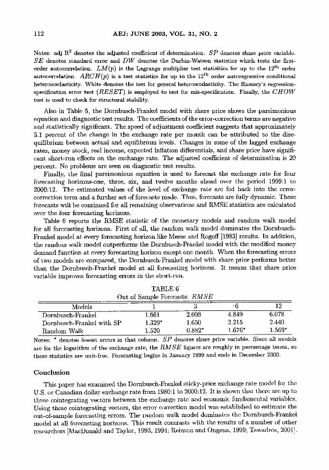
Also in Table 5, the Dornbusch-Frankel model with share price shows the parsimonious equat ion and diagnostic test results. The coefficients of the error-correction terms are negative and statistically significant. The speed of adjustment coefficient suggests tha t approximately 3.1 percent of the change in the exchange rate per month can be a t t r ibuted to the dise- quilibrium between actual and equilibrium levels. Changes in some of the lagged exchange rates, money stock, real income, expected inflation differentials, and share price have signifi- cant short-run effects on the exchange rate. The adjusted coefficient of determinat ion is 20 percent. No problems are seen on diagnostic test results.

Finally, the final parsimonious equation is used to forecast the exchange rate for four forecasting horizons-one, three, six, and twelve months ahead over the period 1999:1 to 2000:12. The est imated values of the level of exchange rate are fed back into the error- correction te rm and a further set of forecasts made. Thus, forecasts are fully dynamic. These forecasts will be continued for all remaining observations and RMSE statistics are calculated over the four forecasting horizons.

Table 6 reports the RMSE statist ic of the monetary models and random walk model for all forecasting horizons. First of all, the random walk model dominates the Dornbusch- Frankel model at every forecasting horizon like Meese and Rogoff [1983] results. In addition, the random walk model outperforms the Dornbusch-Frankel model with the modified money demand function at every forecasting horizon except one month. When the forecasting errors of two models are compared, the Dornbusch-Frankel model with share price performs bet ter than the Dornbusch-Frankel model at all forecasting horizons. I t means tha t share price variable improves forecasting errors in the short-run.

TABLE 6 Out of Sample Forecasts: RMSE

" , . . . . . . . . ' " " '

Models 1 3 ~ 6 12 Dornbusch- Fr ankel 1.661 2.008 4.849 6.078 Dornbusch-Frankel with SP 1.329" L650 2.215 2.440 Random Walk 1.520 0.882* 1.676" 1.569"

Notes: * denotes fewest errors in that column. S P denotes share price variable. Since all models are for the logarithm of the exchange rate, the RMSE figures are roughly in percentage terms, so these statistics are unit-free. Forecasting begins in January 1999 and ends in December 2000.

C o n c l u s i o n

This paper has examined the Dornbusch-Frankel sticky-price exchange rate model for the U.S. or Canadian dollar exchange rate from 1980:1 to 2000:12. I t is shown tha t there are up to three cointegrating vectors between the exchange rate and economic fundamental variables. Using these cointegrating vectors, the error correction model was established to est imate the out-of-sample forecasting errors. The random walk model dominates the Dornbusch-Frankel model a t all forecasting horizons. This result contrasts with the results of a number of other researchers [MacDonald and Taylor, 1993, 1994; Reinton and Ongena, 1999; Tawadros, 2001].

H W A N G : D Y N A M I C F O R E C A S T I N G 113

The random walk model also outperforms the Dornbusch-Frankel model with the modified money demand function at every forecasting horizon except one month. In other words, the Dornbusch-Frankel model with share price predicts exchange rate better than the random walk model at the very short-run horizon. When the forecasting errors of two models are compared, the Dornbusch-Frankel model with share price shows lower forecasting errors than the Dornbusch-Frankel model. The main finding suggests that the share price variable can improve the accuracy of forecasts of exchange rates at short-run horizons.

For the further research, empirical works on more exchange rates might be necessary to support the results of this paper. Also, it would be worth to examine the statistical significance of forecasting accuracy because simply comparing the values of the R M S E does not give any idea of significance of the differences.

F o o t n o t e s

1Goldberg and Frydman [1996] showed that "the large forecasting errors reported in Meese and Rogoff [1983] were the result of allowing the forecasting experiment to run past the end of one exchange rate regime and into the next." They presented that the important factor for the failure of empirical exchange rate models is periodic shifts in the long-run relationship governing the exchange rate and macroeconomic fundamentals.

2The ADF test is comparable to the simple DF test but it involves adding an unknown number of lagged first differences of the dependent variable to capture the autocorrelated omitted variables that would otherwise enter the error term. However, it is very important to select the appropriate lag length; too few lags may result in over-rejecting the null when it is true, while too many lags may reduce the power of the test.

3Another important aspect of diagnostic checking is testing for structural breaks in the model that would be evidence that the parameter estimates are non-constant. The null hypothesis is one of structural stability: coefficients are the same over different subsamples. The break point in January 1985 is also used because the U.S. trade deficit and the dollar had climbed so high by the first quarter of 1984 that the stated Reagan policy was changed to try to get the dollar down.

R e f e r e n c e s

AbdMla, Issam S. A.; Murinde, Victor. "Exchange Rate and Stock Price Interactions in Emerging Financial Markets: Evidence on India, Korea, Pakistan, and the Philippines," Applied Financial Economics, 7, 1997, pp. 25-35.

Ajayi, Richard A.; Mougoue, Mbodja. "On the Dynamic Relation Between Stock Prices and Ex- change Rates," The Journal of Financial Research, 19, 1996, pp. 193-207.

Bahmani-Oskooee, M.; Sohrabian, A. "Stock Prices and the Effective Exchange Rate of the Dollar," Applied Economics, 24, 1992, pp. 459-64.

Baillie, R. J.; Selover, D. D. "Cointegration and Models of Exchange Rate Determination," Interna- tional Yournal of Forecasting, 3, 1987, pp. 43-52.

Boothe, Paul; Olassman, Debra. "Off the Mark: Lessons for Exchange Rate Modeling," Oxford Economic Papers, 39, 1987, pp. 443-57.

Cheung, Yin-Wong; Lai, Kon S. "Long-run Purchasing Power Parity During the Recent Float," Journal of International Economics, 34, 1993, pp. 181-92.

Choudhry, Taufiq. "Real Stock Prices and the Long-run Money Demand Function: Evidence from Canada and the U.S.A.," Journal of International Money and Finance, 15, 1996, pp. 1-17.

Dickey, David; Fuller, Wayne. "Distribution of the Estimator for Autoregressive Time Series with a Unit Root," Journal of American Statistical Association, 74, 1979, pp. 427431.

Dickey, David; Jansen, Dennis; Thornton, Daniel. "A Primer on Cointegration with an Application to Money and Income," Review of Federal Reserve Bank of St. Louis, 73, 1991, pp. 58-78.

114 AEJ : J U N E 2003, VOL. 31, NO. 2

Engle, R. F. "A General Approach to Lagrange Multiplier Model Diagnostic," Journal of Economet- rics, 20, 1982, pp. 83-104.

Engle, R. F.; Granger, C.W. "Co-integration: Representation, Estimation, and Testing," Economet- rica, 55, 1987, pp. 251-76.

Finn, Mary G. "Forecasting the Exchange Rates: A Monetary or Random Walk Phenomenon?" Journal of International Money and Finance, 5, 1986, pp. 181-220.

Friedman, Milton. "Money and the Stock Market," Journal of Political Economy, 96, 1988, pp. 221-45.

Goldberg, Michael D.; Frydman, Roman. "Empirical Exchange Rate Models and Shifts in the Co- integrating Vector," Structural Change and Economics Dynamics, 7, 1996, pp. 55-78.

Johansen, Soren. "Statistical Analysis of Cointegration Vectors," Journal of Economic Dynamics and Control, 12, 1988, pp. 231-54.

Johansen, Soren; Juselius, Katarina. "Maximum Likelihood Estimation and Inference on Cointegration-With Application to the Demand for Money," Oxford Bulletin of Economics and Statistics, 52, 1990, pp. 169-210.

Kwiatkowski, Denis; Phillips, Peter; Schmidt, Peter; Shin, Yongcheol. "Testing the Null Hypothesis of Stationary Against the Alternative of a Unit Root: How Sure Are We That Economic Time Series Have a Unit Root," Journal of Econometrics, 54, 1992, pp. 159-78.

Ma, C. K.; Kao, G.W. "On Exchange Rate Changes and Stock Price Reactions," Journal of Business Finance and Accounting, 17, 1990, pp. 441-49.

MacDonald, R.; Taylor, Mark P. "The Monetary Approach to the Exchange Rate: Rational Expec- tations, Long-run Equilibrium and Forecasting," International Monetary Fund Staff papers, 40, 1993, pp. 89-107.

- - . "The Monetary Model of the Exchange Rate: Long- run Relationships, Short-run Dynamics and How to Beat a Random Walk," Journal of International Money and Finance, 13, 1994, pp. 276-90.

McNown, Robert; Wallace,/vlyles. "Co-integration Tests for Long-run Equilibrium in the Ivlonetary Exchange Rate Model," Economics Letters, 31, 1989, pp. 263-7.

- - . "Cointegration Tests of the Monetary Exchange Rate Model for Three High Inflation Economics," Journal of Money, Credit, and Banking, 26, 1994, pp. 396-411.

Meese, Richard A.; Rogoff, Kenneth. "Empirical Exchange Rate Models of the Seventies: Do They Fit out of Sample?" Journal of International Economics, 14, 1983, pp. 3-74.

Moosa, Imad A. "The Monetary Model of Exchange Rates Revisited," Applied Financial Economics, 26, 1994, pp. 279-87.

Osterwald-Lenum, M. "A Note with Fractiles of the Asymptotic Distribution of the Maximum Likeli- hood Cointegration Rank Test Statistics: Four Cases," Oxford Bulletin of Economics and Statis- tics, 54, 1992, pp. 461-72.

Reinton, H.; Ongena, Steven. "Out-of-Sample Forecasting Performance of Single Equation Monetary Exchange Rate Models in Norwegian Currency Markets," Applied P~nancial Economics, 9, 1999, pp. 545-50.

Smith, C. " Equities and the UK exchange rate," Applied Economics, 24, 1992, pp. 327-35. • Soenen, L.; Henninger, E. "An Analysis of Exchange Rates and Stock Prices-the US Experience

between 1980 and 1986," Akron Business and Economic Review, 19, 1988, pp. 7-16. Sotnik, B. "Using Financial Prices to Test Exchange Rate Models: A Note," Journal of Finance, 42,

1987, pp. 141-9. Somanath, V. S. "Efficient Exchange Rate Forecast: Lagged Models Better than the Random W*alk,"

Journal of International Money and Finance, 5, 1986, pp. 195-220. Tawadros, George. "The Predictive Power of the Monetary Model of Exchange Rate Determination,"

Applied Financial Economics, 11, 2001, pp. 279-86. Wnnite, H. "A Heteroskedasticity-Consistent Covariance Matrix and a Direct Test for Heteroskedas-

ticity," Eeonometrica, 48, 1980, pp. 721-46. Woo, Wing T. "The Monetary Approach to Exchange Rate Determination under Rational Expec-

tations," Journal of International Economics, 18, 1985, pp. 1-16,