Dynamic Factor Models

January 2010 This revision: May 7, 2010

James H. Stock

Department of Economics, Harvard University and the National Bureau of Economic Research

and

Mark W. Watson*

Woodrow Wilson School and Department of Economics, Princeton University

and the National Bureau of Economic Research

*Prepared for the Oxford Handbook of Economic Forecasting, Michael P. Clements and David F. Hendry (eds), Oxford University Press. We thank Jushan Bai and Serena Ng for helpful discussions and Ugo Troiano for research assistance.

1

1. Introduction

Macroeconometricians face a peculiar data structure. On the one hand, the

number of years for which there is reliable and relevant data is limited and cannot readily

be increased other than by the passage of time. On the other hand, for much of the

postwar period statistical agencies have collected monthly or quarterly data on a great

many related macroeconomic, financial, and sectoral variables. Thus

macroeconometricians face data sets that have hundreds or even thousands of series, but

the number of observations on each series is relatively short, for example 20 to 40 years

of quarterly data.

This chapter surveys work on a class of models, dynamic factor models (DFMs),

which has received considerable attention in the past decade because of their ability to

model simultaneously and consistently data sets in which the number of series exceeds

the number of time series observations. Dynamic factor models were originally proposed

by Geweke (1977) as a time-series extension of factor models previously developed for

cross-sectional data. In early influential work, Sargent and Sims (1977) showed that two

dynamic factors could explain a large fraction of the variance of important U.S. quarterly

macroeconomic variables, including output, employment, and prices. This central

empirical finding that a few factors can explain a large fraction of the variance of many

macroeconomic series has been confirmed by many studies; see for example Giannone,

Reichlin, and Sala (2004) and Watson (2004).

The aim of this survey is to describe, at a level that is specific enough to be useful

to researchers new to the area, the key theoretical results, applications, and empirical

findings in the recent literature on DFMs. Bai and Ng (2008) and Stock and Watson

2

(2006) provide complementary surveys of this literature. Bai and Ng’s (2008) survey is

more technical than this one and focuses on the econometric theory and conditions; Stock

and Watson (2006) focus on DFM-based forecasts in the context of other methods for

forecasting with many predictors.

The premise of a dynamic factor model is that a few latent dynamic factors, ft,

drive the comovements of a high-dimensional vector of time-series variables, Xt, which is

also affected by a vector of mean-zero idiosyncratic disturbances, et. These idiosyncratic

disturbances arise from measurement error and from special features that are specific to

an individual series (the effect of a Salmonella scare on restaurant employment, for

example). The latent factors follow a time series process, which is commonly taken to be

a vector autoregression (VAR). In equations, the dynamic factor model is,

Xt = λ(L)ft + et (1)

ft = Ψ(L)ft–1 + ηt (2)

where there are N series, so Xt and et are N×1, there are q dynamic factors so ft and ηt are

q×1, L is the lag operator, and the lag polynomial matrices λ(L) and Ψ(L) are N×q and

q×q, respectively. The ith lag polynomial λi(L) is called the dynamic factor loading for

the ith series, Xit, and λi(L)ft is called the common component of the ith series. We assume

that all the processes in (1) and (2) are stationary (nonstationarity is discussed in the final

section of this chapter). The idiosyncratic disturbances are assumed to be uncorrelated

with the factor innovations at all leads and lags, that is, Eetηt–k′ = 0 for all k. In the so-

called exact dynamic factor model, the idiosyncratic disturbances are assumed to be

mutually uncorrelated at all leads and lags, that is, Eeitejs = 0 for all s if i ≠ j.

3

An important motivation for considering DFMs is that, if one knew the factors ft

and if (et, ηt) are Gaussian, then one can make efficient forecasts for an individual

variable using the population regression of that variable on the lagged factors and lags of

that variable. Thus the forecaster gets the benefit of using all N variables by using only q

factors, where q is typically much smaller than N. Specifically, under squared error loss,

the optimal one-step ahead forecast of the ith variable is,

E[Xit+1| Xt, ft, Xt–1, ft–1,…] = E[λi(L)ft+1 + eit+1| Xt, ft, Xt–1, ft–1,…]

= E[λi(L)ft+1| Xt, ft, Xt–1, ft–1,…] + E[eit+1| Xt, ft, Xt–1, ft–1,…]

= E[λi(L)ft+1| ft, ft–1,…] + E[eit+1| eit, eit–1, …]

= α(L)ft + δ(L)Xit, (3)

where the third line follows from (2) and the final line follows from (1) and the exact

DFM assumptions. Thus the dimension of the efficient population forecasting regression

does not increase as one adds variables to the system.

The first issue at hand for the econometrician is to estimate the factors (or, more

precisely, to estimate the space spanned by the factors) and to ascertain how many factors

there are; these two topics are covered in the Sections 2 and 3 of this survey. Once one

has reliable estimates of the factors in hand, there are a number of things one can do with

them beyond using them for forecasting, including using them as instrumental variables,

estimating factor-augmented vector autoregressions (FAVARs), and estimating dynamic

stochastic general equilibrium models (DSGEs); these applications are covered in

Section 4. Section 5 discusses some extensions.

4

2. Factor Estimation

The seminal work of Geweke (1977) and Sargent and Sims (1977) used frequency

domain methods to look for evidence of a dynamic factor structure and to estimate the

importance of the factor. Those methods, however, could not estimate ft directly and thus

could not be used for forecasting. Therefore subsequent work on DFMs focused on time-

domain methods in which ft could be estimated directly.

Work on time-domain estimation of DFMs can be divided into three generations.

The first generation consisted of low-dimensional (small N) parametric models estimated

in the time domain using Gaussian maximum likelihood estimation (MLE) and the

Kalman filter. This method provides optimal estimates of f (and optimal forecasts) under

the model assumptions and parameters. However, estimation of those parameters entails

nonlinear optimization, which historically had the effect of restricting the number of

parameters, and thus the number of series, that could be handled. The second generation

of estimators entailed nonparametric estimation with large N using cross-sectional

averaging methods, primarily principal components and related methods. The key result

in this second generation is that the principal components estimator of the space spanned

by the factors is consistent and moreover, if N is sufficiently large, then the factors are

estimated precisely enough to be treated as data in subsequent regressions. The third

generation uses these consistent nonparametric estimates of the factors to estimate the

parameters of the state space model used in the first generation and thereby solves the

dimensionality problem associated encountered by first-generation models. A different

solution to the problem of the very many unknown parameters in the state space model is

to use Bayesian methods, that is, to specify a prior and integrate instead of maximize, and

5

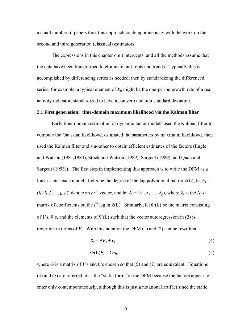
a small number of papers took this approach contemporaneously with the work on the

second and third generation (classical) estimators.

The expressions in this chapter omit intercepts, and all the methods assume that

the data have been transformed to eliminate unit roots and trends. Typically this is

accomplished by differencing series as needed, then by standardizing the differenced

series; for example, a typical element of Xit might be the one-period growth rate of a real

activity indicator, standardized to have mean zero and unit standard deviation.

2.1 First generation: time-domain maximum likelihood via the Kalman filter

Early time-domain estimation of dynamic factor models used the Kalman filter to

compute the Gaussian likelihood, estimated the parameters by maximum likelihood, then

used the Kalman filter and smoother to obtain efficient estimates of the factors (Engle

and Watson (1981,1983), Stock and Watson (1989), Sargent (1989), and Quah and

Sargent (1993)). The first step in implementing this approach is to write the DFM as a

linear state space model. Let p be the degree of the lag polynomial matrix λ(L), let Ft =

(ft′, ft–1′,…, ft–p′)′ denote an r×1 vector, and let Λ = (λ0, λ1,…, λp), where λi is the N×q

matrix of coefficients on the ith lag in λ(L). Similarly, let Φ(L) be the matrix consisting

of 1’s, 0’s, and the elements of Ψ(L) such that the vector autoregression in (2) is

rewritten in terms of Ft. With this notation the DFM (1) and (2) can be rewritten,

Xt = ΛFt + et (4)

Φ(L)Ft = Gηt, (5)

where G is a matrix of 1’s and 0’s chosen so that (5) and (2) are equivalent. Equations

(4) and (5) are referred to as the “static form” of the DFM because the factors appear to

enter only contemporaneously, although this is just a notational artifact since the static

6

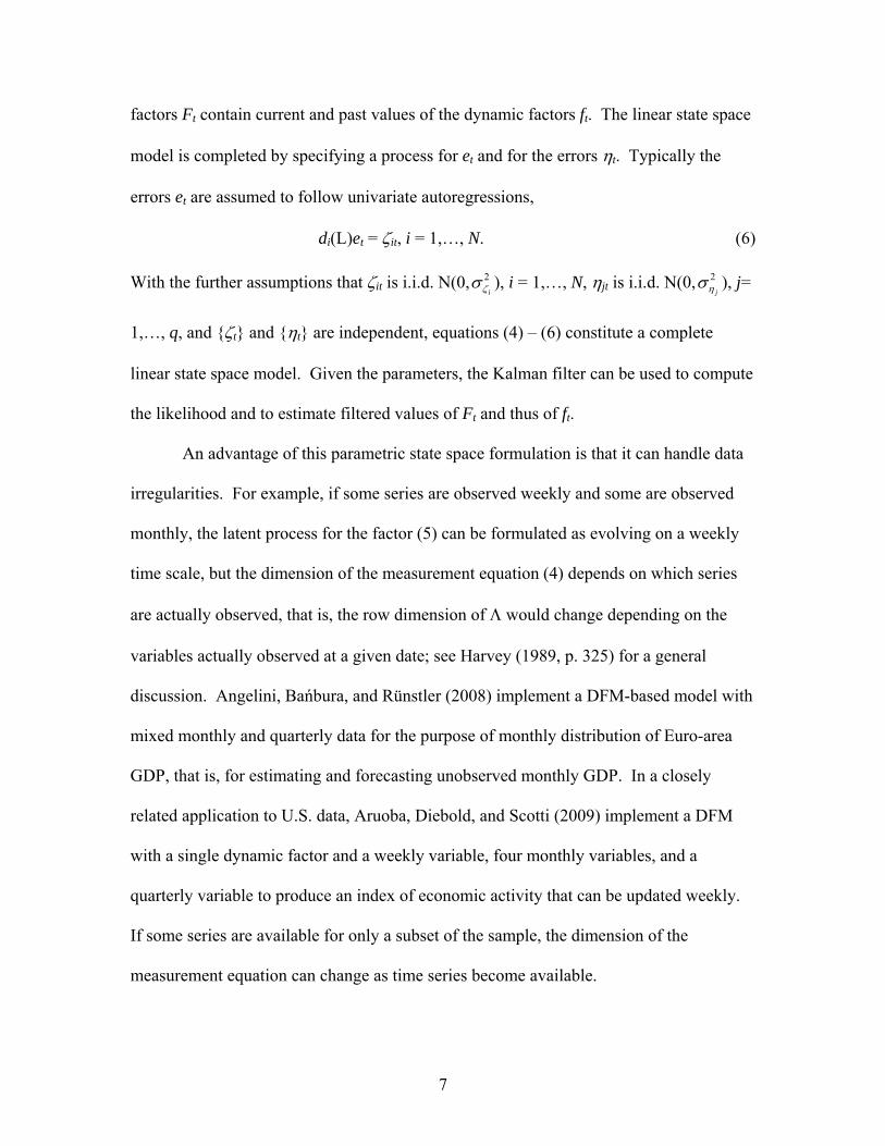
factors Ft contain current and past values of the dynamic factors ft. The linear state space

model is completed by specifying a process for et and for the errors ηt. Typically the

errors et are assumed to follow univariate autoregressions,

di(L)et = ζit, i = 1,…, N. (6)

With the further assumptions that ζit is i.i.d. N(0, 2iζ

σ ), i = 1,…, N, ηjt is i.i.d. N(0, 2jησ ), j=

1,…, q, and {ζt} and {ηt} are independent, equations (4) – (6) constitute a complete

linear state space model. Given the parameters, the Kalman filter can be used to compute

the likelihood and to estimate filtered values of Ft and thus of ft.

An advantage of this parametric state space formulation is that it can handle data

irregularities. For example, if some series are observed weekly and some are observed

monthly, the latent process for the factor (5) can be formulated as evolving on a weekly

time scale, but the dimension of the measurement equation (4) depends on which series

are actually observed, that is, the row dimension of Λ would change depending on the

variables actually observed at a given date; see Harvey (1989, p. 325) for a general

discussion. Angelini, Bańbura, and Rünstler (2008) implement a DFM-based model with

mixed monthly and quarterly data for the purpose of monthly distribution of Euro-area

GDP, that is, for estimating and forecasting unobserved monthly GDP. In a closely

related application to U.S. data, Aruoba, Diebold, and Scotti (2009) implement a DFM

with a single dynamic factor and a weekly variable, four monthly variables, and a

quarterly variable to produce an index of economic activity that can be updated weekly.

If some series are available for only a subset of the sample, the dimension of the

measurement equation can change as time series become available.

7

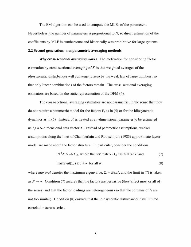
The EM algorithm can be used to compute the MLEs of the parameters.

Nevertheless, the number of parameters is proportional to N, so direct estimation of the

coefficients by MLE is cumbersome and historically was prohibitive for large systems.

2.2 Second generation: nonparametric averaging methods

Why cross-sectional averaging works. The motivation for considering factor

estimation by cross-sectional averaging of Xt is that weighted averages of the

idiosyncratic disturbances will converge to zero by the weak law of large numbers, so

that only linear combinations of the factors remain. The cross-sectional averaging

estimators are based on the static representation of the DFM (4).

The cross-sectional averaging estimators are nonparametric, in the sense that they

do not require a parametric model for the factors Ft as in (5) or for the idiosyncratic

dynamics as in (6). Instead, Ft is treated as a r-dimensional parameter to be estimated

using a N-dimensional data vector Xt. Instead of parametric assumptions, weaker

assumptions along the lines of Chamberlain and Rothschild’s (1983) approximate factor

model are made about the factor structure. In particular, consider the conditions,

N-1Λ′Λ → DΛ, where the r×r matrix DΛ has full rank, and (7)

maxeval(Σe) ≤ c < ∞ for all N , (8)

where maxeval denotes the maximum eigenvalue, Σe = Eetet′, and the limit in (7) is taken

as N → ∞ Condition (7) assures that the factors are pervasive (they affect most or all of

the series) and that the factor loadings are heterogeneous (so that the columns of Λ are

not too similar). Condition (8) ensures that the idiosyncratic disturbances have limited

correlation across series.

8

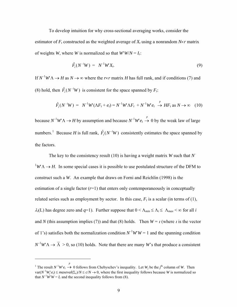
To develop intuition for why cross-sectional averaging works, consider the

estimator of Ft constructed as the weighted average of Xt using a nonrandom N×r matrix

of weights W, where W is normalized so that W′W/N = Ir:

1ˆ (tF N W− )

)

= N–1W′Xt. (9)

If N–1W′Λ → H as N → ∞ where the r×r matrix H has full rank, and if conditions (7) and

(8) hold, then 1ˆ (tF N W− is consistent for the space spanned by Ft:

1ˆ (tF N W− )

)

= N–1W′(ΛFt + et) = N–1W′ΛFt + N–1W′et HFt as N → ∞ (10) p→

because N–1W′Λ → H by assumption and because N–1W′et 0 by the weak law of large

numbers.

p→

1 Because H is full rank, consistently estimates the space spanned by

the factors.

1ˆ (tF N W−

The key to the consistency result (10) is having a weight matrix W such that N–

1W′Λ → H. In some special cases it is possible to use postulated structure of the DFM to

construct such a W. An example that draws on Forni and Reichlin (1998) is the

estimation of a single factor (r=1) that enters only contemporaneously in conceptually

related series such as employment by sector. In this case, Ft is a scalar (in terms of (1),

λi(L) has degree zero and q=1). Further suppose that 0 < Λmin ≤ Λi ≤ Λmax < ∞ for all i

and N (this assumption implies (7)) and that (8) holds. Then W = ι (where ι is the vector

of 1’s) satisfies both the normalization condition N–1W′W = 1 and the spanning condition

N–1W′Λ → Λ > 0, so (10) holds. Note that there are many W’s that produce a consistent

1 The result N–1W′et 0 follows from Chebyschev’s inequality. Let Wj be the jth column of W. Then var(N–1Wj′et) ≤ maxeval(Σe)/N ≤ c/N → 0, where the first inequality follows because W is normalized so that N–1W′W = Ir and the second inequality follows from (8).

p→

9

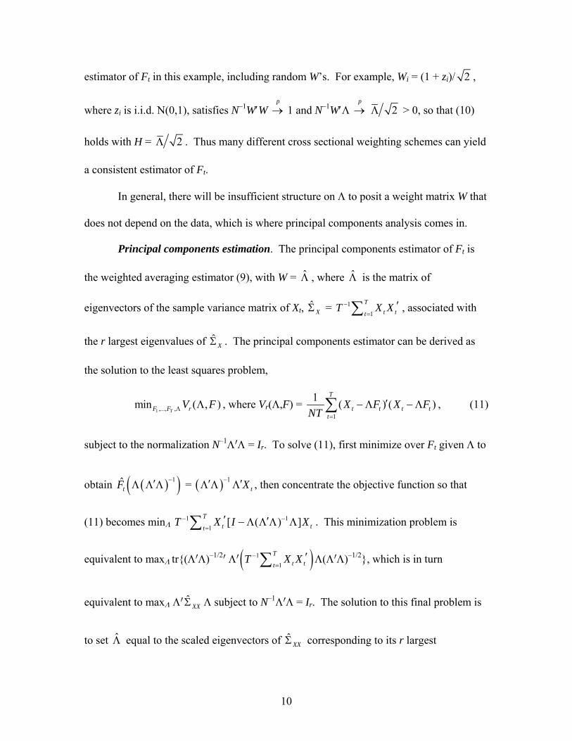
estimator of Ft in this example, including random W’s. For example, Wi = (1 + zi)/ 2 ,

where zi is i.i.d. N(0,1), satisfies N–1W′W 1 and N–1W′Λ p→

p→ 2Λ > 0, so that (10)

holds with H = 2Λ . Thus many different cross sectional weighting schemes can yield

a consistent estimator of Ft.

In general, there will be insufficient structure on Λ to posit a weight matrix W that

does not depend on the data, which is where principal components analysis comes in.

Principal components estimation. The principal components estimator of Ft is

the weighted averaging estimator (9), with W = Λ , where Λ is the matrix of

eigenvectors of the sample variance matrix of Xt, ˆXΣ = 1−

1 t tXT

tT

=∑ X ′ , associated with

the r largest eigenvalues of . The principal components estimator can be derived as

the solution to the least squares problem,

ˆXΣ

1 ,..., ,min ( , )TF F rV FΛ Λ , where Vr(Λ,F) =

1

1 ( ) (T

t t tt

)tX F X FNT =

′− Λ − Λ∑ , (11)

subject to the normalization N–1Λ′Λ = Ir. To solve (11), first minimize over Ft given Λ to

obtain = ( )( )1tF −′Λ Λ Λ ( ) 1

tX−′ ′Λ Λ Λ

11

[ (T

tT X I−

=′ − Λ∑

′Λ)–1/2′ Λ′

, then concentrate the objective function so that

(11) becomes m ] tX . This minimization problem is

equivalent to maxΛ tr{(Λ

inΛ 1−)t Λ Λ′Λ

( )1

Tt tt

X X=

1T − ′∑ Λ(Λ′Λ)–1/2}, which is in turn

equivalent to maxΛ Λ′ ˆXXΣ Λ subject to N–1Λ′Λ = Ir. The solution to this fina problem is

to set Λ equal to the scaled eigenvectors of ˆXX

l

Σ corresponding to its r largest

10

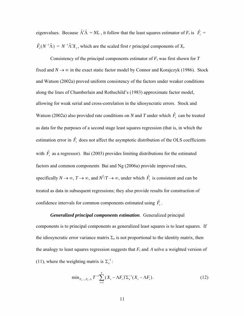
eigenvalues. Because ˆ ˆ′Λ Λ = NIr , it follow that the leas qua ator

1ˆ ˆ( )tF N − Λ = 1 ˆtN X− ′Λ , which are the scaled first r princi

t s res estim of Ft is =

pal components of Xt.

tF

Consistency of the principal components estimator of Ft was first shown for T

fixed and N → ∞ in the exact static factor model by Connor and Korajczyk (1986). Stock

and Watson (2002a) proved uniform consistency of the factors under weaker conditions

along the lines of Chamberlain and Rothschild’s (1983) approximate factor model,

allowing for weak serial and cross-correlation in the idiosyncratic errors. Stock and

Watson (2002a) also provided rate conditions on N and T under which can be treated

as data for the purposes of a second stage least squares regression (that is, in which the

estimation error in does not affect the asymptotic distribution of the OLS coefficients

with

tF

tF

tF as a regressor). Bai (2003) provides limiting distributions for the estimated

factors and common components Bai and Ng (2006a) provide improved rates,

specifically N → ∞, T → ∞, and N2/T → ∞, under which is consistent and can be

treated as data in subsequent regressions; they also provide results for construction of

confidence intervals for common components estimated using

tF

tF .

Generalized principal components estimation. Generalized principal

components is to principal components as generalized least squares is to least squares. If

the idiosyncratic error variance matrix Σe is not proportional to the identity matrix, then

the analogy to least squares regression suggests that F and Λ solve a weighted version of t

(11), where the weighting matrix is 1e−Σ :

1

1 1,..., ,

1( ) ( )

T

T

F F t t e t tt

T X F X F− −Λ

=

′− Λ Σ −Λ∑ . (12) min

11

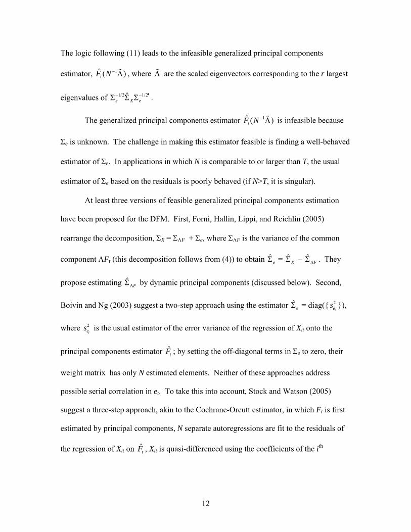
The logic following (11) leads to the infeasible generalized principal components

estimator, , where Λ are the scaled eigenvectors corresponding to the r largest

eigenvalues of .

1ˆ (tF N − Λ

1/2 ˆΣ Σ

)

)

1/2e X e− − ′Σ

The generalized principal components estimator 1ˆ (tF N − Λ is infeasible because

Σe is unknown. The challenge in making this estimator feasible is finding a well-behaved

estimator of Σe. In applications in which N is comparable to or larger than T, the usual

estimator of Σe based on the residuals is poorly behaved (if N>T, it is singular).

At least three versions of feasible generalized principal components estimation

have been proposed for the DFM. First, Forni, Hallin, Lippi, and Reichlin (2005)

rearrange the decomposition, ΣX = ΣΛF + Σe, where ΣΛF is the variance of the common

component ΛFt (this decomposition follows from (4)) to obtain ˆeΣ = ˆ

XΣ – . They

propose estimating by dynamic principal components (discussed below). Second,

Boivin and Ng (2003) suggest a two-step approach using the estimator = diag({ }),

where is the usual estimator of the error variance of the regression of Xit onto the

principal components estimator

ˆFΛΣ

ˆFΛΣ

ˆeΣ

2ies

2ies

tF ; by setting the off-diagonal terms in Σe to zero, their

weight matrix has only N estimated elements. Neither of these approaches address

possible serial correlation in et. To take this into account, Stock and Watson (2005)

suggest a three-step approach, akin to the Cochrane-Orcutt estimator, in which Ft is first

estimated by principal components, N separate autoregressions are fit to the residuals of

the regression of Xit on , Xit is quasi-differenced using the coefficients of the ith tF

12

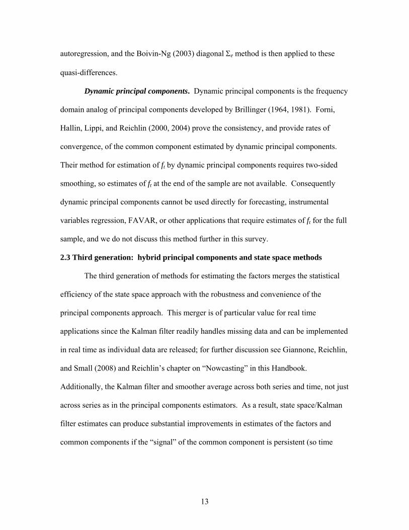
autoregression, and the Boivin-Ng (2003) diagonal Σe method is then applied to these

quasi-differences.

Dynamic principal components. Dynamic principal components is the frequency

domain analog of principal components developed by Brillinger (1964, 1981). Forni,

Hallin, Lippi, and Reichlin (2000, 2004) prove the consistency, and provide rates of

convergence, of the common component estimated by dynamic principal components.

Their method for estimation of ft by dynamic principal components requires two-sided

smoothing, so estimates of ft at the end of the sample are not available. Consequently

dynamic principal components cannot be used directly for forecasting, instrumental

variables regression, FAVAR, or other applications that require estimates of ft for the full

sample, and we do not discuss this method further in this survey.

2.3 Third generation: hybrid principal components and state space methods

The third generation of methods for estimating the factors merges the statistical

efficiency of the state space approach with the robustness and convenience of the

principal components approach. This merger is of particular value for real time

applications since the Kalman filter readily handles missing data and can be implemented

in real time as individual data are released; for further discussion see Giannone, Reichlin,

and Small (2008) and Reichlin’s chapter on “Nowcasting” in this Handbook.

Additionally, the Kalman filter and smoother average across both series and time, not just

across series as in the principal components estimators. As a result, state space/Kalman

filter estimates can produce substantial improvements in estimates of the factors and

common components if the “signal” of the common component is persistent (so time

13

averaging helps) and small (so substantial noise remains after cross-series averaging); for

an empirical example see Reiss and Watson (2010).

This merged estimation procedure occurs in two steps, which are described in

more detail in Giannone, Reichlin, and Small (2008) and Doz, Giannone, and Reichlin

(2006). First, the factors are estimated by principal components or generalized principal

components. In the second step, these estimated factors are used to estimate the

unknown parameters of the state space representation. The specifics of how to do this

depend on whether the state vector is specified in terms of the static or dynamic factors.

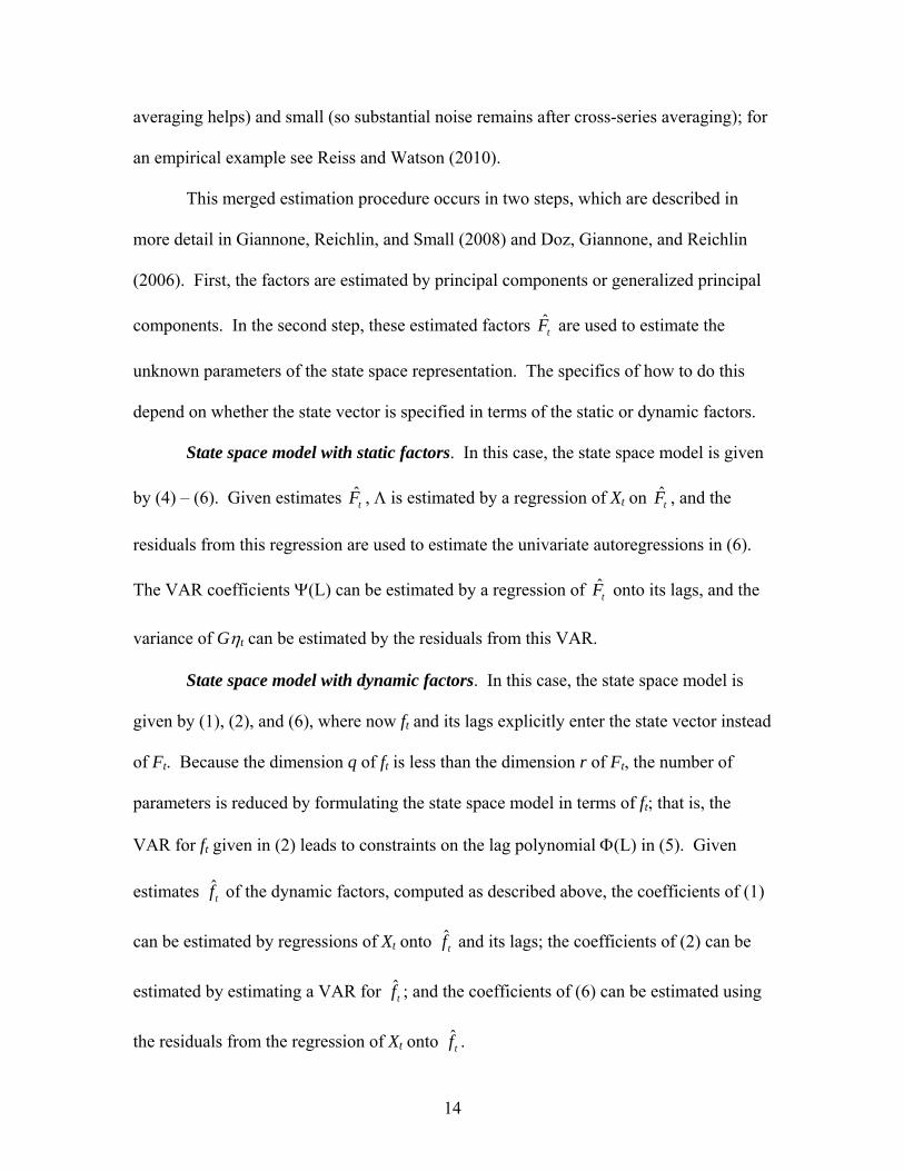
tF

State space model with static factors. In this case, the state space model is given

by (4) – (6). Given estimates tF , Λ is estimated by a regression of Xt on tF , and the

residuals from this regression are used to estimate the univariate autoregressions in (6).

The VAR coefficients Ψ(L) can be estimated by a regression of onto its lags, and the

variance of Gηt can be estimated by the residuals from this VAR.

tF

State space model with dynamic factors. In this case, the state space model is

given by (1), (2), and (6), where now ft and its lags explicitly enter the state vector instead

of Ft. Because the dimension q of ft is less than the dimension r of Ft, the number of

parameters is reduced by formulating the state space model in terms of ft; that is, the

VAR for ft given in (2) leads to constraints on the lag polynomial Φ(L) in (5). Given

estimates tf of the dynamic factors, computed as described above, the coefficients of (1)

can be estimated by regressions of Xt onto tf and its lags; the coefficients of (2) can be

estimated by estimating a VAR for tf ; and the coefficients of (6) can be estimated using

the residuals from the regression of Xt onto tf .

14

These estimated parameters fully populate the state space model so that an

improved estimate of Ft or ft, which now invokes time-series averaging, can be computed

using the Kalman smoother.

It is also possible to use these estimated coefficients as consistent starting values

for maximum likelihood estimation of the coefficients. The MLEs can be computed

using the EM algorithm, see for example Engle and Watson (1983), Quah and Sargent

(1993) and Doz, Giannone, and Reichlin (2006). Jungbacker and Koopman (2008) show

how to speed up the evaluation of the Kalman filter in the DFM by transforming the Xt

into an r×1 vector. Jungbacker, Koopman, and van der Wel (2009) provide additional

computational devices that can be used when there are missing data.

2.4 Comparisons of estimators

Several studies have compared the performance of principal components

estimators and various feasible generalized principal components estimators in Monte

Carlo exercises and in forecast comparisons with actual data. The studies reach

somewhat different conclusions when N is small, presumably because the study designs

differ. Forni, Hallin, Lippi, and Reichlin (2005) find, in a Monte Carlo study, that their

generalized principal components estimator is substantially more precise than the

principal components estimator of the common component when there are persistent

dynamics in the factors and in the idiosyncratic disturbances, although these differences

disappear for large N and T. In contrast, Boivin and Ng (2005), using a Monte Carlo

design calibrated to U.S. data, find only minor differences between the principal

components and Forni et. al. (2005) generalized principal components estimators.

15

Boivin and Ng (2005) and D’Agostino and Giannone (2006) also compare the

forecasting performance of the principal components estimator to various feasible

generalized principal components estimators. Although there are nuances, the

overarching conclusion of these comparisons is that the forecasts produced using the

various estimators of the factors are highly collinear (holding constant the forecast

specification and changing only the factor estimator), and produce very similar R2s.

There is some evidence that the generalized principal components estimators produce

more variable forecasts (sometimes better, sometimes worse) than principal components

when N is small, but for values of N and T typical of applied work there is negligible

difference in the performance, as measured by pseudo out-of-sample mean squared error,

among the forecasts based on the various estimators. This result reassuringly accords

with the intuition provided at the beginning of this section, that there is no unique weight

matrix W that produces a consistent estimator of the factors, ; rather, sufficient

conditions for consistency are that W′Λ → H, where H is full rank, and that W′ΣeW → 0.

ˆ ( )tF W

2.5 Bayes estimation

The DFM parameters and factors also can be estimated using Bayesian methods.

Historically, there are three main motivations for using Bayes methods to estimate

DFMs: first, integration to compute the posterior can be numerically easier and more

stable than maximizing the likelihood when there are very many unknown parameters;

second, Markov Chain Monte Carlo methods can be used to compute posteriors in

nonlinear/nonGaussian latent variable models in which it is exceedingly difficult to

compute the likelihood directly; and third, some analysts might wish to impose a-priori

information on the model in the form of a prior distribution. The first two of these

16

motivations, however, are less relevant today, at least for DFM applications with large N

and relatively few factors: the second-generation nonparametric estimators sidestep the

numerical challenges of brute-force MLE and allow the factors and idiosyncratic terms to

follow nonlinear and/or nonGaussian processes, and the third-generation methods refine

these nonparametric estimates using a high-dimensional parametric state-space model.

Bayes estimation of the DFM parameters and the factor are based on Markov

Chain Monte Carlo methods. Chib and Greenberg (1996) lay out the basics of Gibbs

sampling applied to linear/Gaussian state space models. Otrok and Whiteman (1996)

provide an early implementation of these methods to a linear/Gaussian DFM in state

space, in which they estimate a single dynamic factor using four variables. Kose, Otrok,

and Whiteman (2003, 2008) use these methods to characterize international

comovements and to study international transmission of economic shocks; Kose, Otrok,

and Whiteman’s (2008) model has 7 common factors among 60 countries, with 3 series

per country (so N = 180) and T = 30 annual observations. Bernanke, Boivin, and Eliasz

(2005) use Gibbs sampling to estimate a state-space version of a Factor Augmented

Vector Autoregression (FAVAR, discussed below), but they report that doing so provides

only modest changes relative to a second-generation estimation approach in which

principle components estimates of the factors are treated as data. Boivin and Giannoni

(2006) use Markov Chain Monte Carlo methods to estimate the parameters of a dynamic

stochastic general equilibrium (DSGE) model for the latent factors, that is, a model for

Ψ(L) and var(ηt) in (2), which are measured by observable series, thus imposing structure

on λ(L) to identify the factors. In Boivin and Giannoni’s (2006) application, and in the

17

DSGE literature more generally, the priors serve to overcome what appears to be a lack

of identification or weak identification of some of the DSGE parameters.

Although the focus of this chapter is the linear DFM, with Gaussian errors when

treated parametrically, Bayesian methods are particularly useful when the model contains

nonlinear and/or nonGaussian elements. For example, Kim and Nelson (1998) estimate a

four-variable DFM in which a single latent factor has a mean that follows a latent

Hamilton (1989) Markov switching (regime switching) process. The Hamilton (1989)

filter does not extend to this case, that is, for this model, closed-form expressions for the

integrals in the general nonlinear/nonGaussian filter in Kitagawa (1987) are not known.

The hierarchical nature of this model, however, lends itself to Gibbs sampling and thus to

computation of the posterior distribution of the model parameters and the dynamic factor.

Carlin, Polson and Stoffer (1992) lay out the general MCMC approach for

nonlinear/nonGaussian state space models. It should be noted, however, that in a large-N

context, the difficulties posed by the nonlinear/nonGaussian structure for the factors in

Kim and Nelson (1998) are also handled by second-generation classical methods. For

example, if N is large then tF can be treated as data and the original Hamilton (1989)

switching model can be applied instead of using the Kim and Nelson (1998) method,

although we are not aware of an application that does so.

A practical motivation for using Bayes methods would be that they produce better

forecasts than second- or third-generation classical methods, however we are not aware

of a study that undertakes such a comparison.

18

3. Determining the Number of Factors

Several methods are available for estimating the number of static factors r and the

number of dynamic factors q.

3.1 Estimating the number of static factors r

The number of static factors r can be determined by a combination of a-priori

knowledge, visual inspection of a scree plot, and the use of information criteria

developed by Bai and Ng (2002).

Scree plots as a visual diagnostic. A scree plot, introduced by Catell (1966), is a

plot of the ordered eigenvalues of ˆXΣ against the rank of that eigenvalues. Scree plots

are useful diagnostic measures that allow one to assess visually the marginal contribution

of the ith principal component to the (trace) R2 of the regression of Xt against the first i

principal components. The scree plot is a useful visual diagnostic; formal tests based on

scree plots are discussed below.

Estimation of r based on information criteria. Bai and Ng (2002) developed a

family of estimators of r that are motivated by information criteria used in model

selection. Information criteria trade off the benefit of including an additional factor (or,

more generally, an additional parameter in a model) against the cost of increased

sampling variability arising from estimating another parameter. This is done by

minimizing a penalized likelihood or log sum of squares, where the penalty factor

increases linearly in the number of factors (or parameters). In the DFM case, Bai and Ng

(2002) propose minimizing the penalized sum of squares,

IC(r) = lnVr( , ) + rg(N,T), (13) Λ F

19

where Vr( , ) is the least squares objective function in Λ F (11), evaluated at the principal

components estimators ( , ), and where g(N,T) is a penalty factor such that g(N,T) →

0 and min(N,T)g(N,T) → ∞ as N, T → ∞. These latter conditions are the generalizations

to N, T → ∞ of the standard conditions for the consistency of information criteria in

regression, see for example Geweke and Meese (1981). Bai and Ng (2002, 2006b) show

that, under the conditions of the approximate DFM, the value of r, , that minimizes an

information criterion with g(N,T) satisfying these conditions is consistent for the true

value of r, assuming that value of r is finite and does not increase with (N, T).

Λ F

r

A specific choice for g(N,T) that does well in simulations (e.g. Bai and Ng

(2002)) is g(N,T) = (N+T)ln(min(N,T))/(NT). In the special case N = T this g(N,T)

simplifies to two times the familiar BIC penalty factor, that is, g(T, T) = 2T–1lnT. Bai

and Ng (2002) refer to the information criterion as ICp2.

Ahn and Horenstein (2009) build on the theoretical results in Bai-Ng (2002) and

propose estimating r as the maximizer of the ratio of adjoining eigenvalues; intuitively,

this corresponds to finding the edge of the cliff in the scree plot. Their Monte Carlo

simulation suggests that this might be a promising new approach that sidesteps a

somewhat arbitrary choice about which penalty factor to use in the Bai-Ng (2002)

information criterion approach.

Formal tests based on scree plots. Formal distribution theory for the scree plot,

and in particular for how to test for whether a seemingly large eigenvalue is in fact large

enough to indicate the presence of latent factors, is well known for the special case that,

under the null hypothesis, Xit is i.i.d. N(0,1); however a general theory of scree plots has

only recently been developed. In the special case that Xit is i.i.d. standard normal, then

20

the eigenvalues are those of a Wishart distribution (see Anderson (1984)). If in addition

N, T → ∞, the largest (centered and rescaled) eigenvalue has the Tracy-Widom (1994)

distribution (Johnstone (2001)); this finding means that one need not use the exact

Wishart distribution, which depends on (N, T). El Karoui (2007) generalizes Johnstone

(2001) to the case that {Xit, t = 1,…, T} is serially correlated but independent over i,

subject to the condition that all series i = 1,…, N have the same spectrum which satisfies

certain smoothness conditions. Onatski (2008) extends El Karoui (2007) to provide a

joint limit (a vector Tracy-Widom law) for the centered and rescaled first several

eigenvalues. Because the problem is symmetric in N and T, this result applies equally to

panels with cross-sectional correlation but no time series dependence. Onatski (2009)

uses the results in Onatski (2008) to develop a pivotal statistic that can be used to test the

hypothesis that q = q0 against the hypothesis that q > q0. Onatski’s (2009) test is in the

spirit of Brillinger’s generalized principal components analysis in that it looks at a

function of the eigenvalues of the smoothed spectral density matrix at a given frequency,

where the function is chosen so that the test statistic is pivotal.

3.2 Estimating the number of dynamic factors q

Three methods have been proposed for formal estimation of the number of

dynamic factors. Hallin and Liška (2007) propose a frequency-domain procedure based

on the observation that the rank of the spectrum of the common component of Xt is q.

Bai and Ng (2007) propose an estimator based on the observation that the innovation

variance matrix in the population VAR (5) has rank q. Their procedure entails first

estimating the sample VAR by regressing the principal components estimator tF on its

lags, then comparing the eigenvalues of the residual variance matrix from this VAR to a

21

shrinking bound that depends on (N, T). Amenguel and Watson’s (2007) estimator is

based on noting that, in a regression of Xt on past values of Ft, the residuals have a factor

structure with rank q; they show that the Bai-Ng (2002) information criterion, applied to

the sample variance matrix of these residuals, yields a consistent estimate of the number

of dynamic factors. Our own limited Monte Carlo experiments suggest that the Bai-Ng

(2007) has somewhat better finite sample performance than the Amenguel-Watson (2007)

procedure. We are not aware of a third-party evaluation and comparison of these

competing procedures, and such a study is in order.

4. Uses of the Estimated Factors

The estimated factors can be used as data in second-stage regressions and they

can be used to estimate structural models, both structural factor-augmented vector

autoregressions and DSGEs.

4.1 Use of factors in second stage regressions

Forecasting. As motivated by (3), one step ahead forecasts of a variable yt

(which may or may not be an element of Xt used to estimate the factors) can be computed

by regressing yt+1 on tF , yt, lags of yt, and (optionally) additional lags of tF . Multistep

(that is, h-step ahead) forecasts can be computed in two ways. Direct multistep forecasts

are computed by regressing yt+h on tF , yt, and their lags. Alternatively, iterated multistep

forecasts can be computed by first estimating a VAR for , then using this VAR in

conjunction with the one-step ahead forecasting equation to iterate forward h periods. In

theory, either direct or iterated forecasts could be better, direct because they avoid

potential misspecification error in the VAR for y and F, indirect because they are more

tF

22

efficient if the VAR model is correctly specified. Empirical evidence provided by Boivin

and Ng (2005) for U.S. macro data suggests that the direct method outperforms the

iterated method, perhaps (they suggest) because the direct method avoids the risk of

misspecification of the process driving the factors. Interestingly, this stands in contrast to

Marcellino, Stock, and Watson’s (2006) finding that iterated forecasts tend to outperform

direct forecasts for models (univariate autoregressions and bivariate ARs) estimated using

U.S. macro data. An alternative method for computing iterated forecasts is to iterating

forward the state space model, estimated using a hybrid method and the Kalman filter.

This has potential advantages over iterating forward a VAR estimated with because

the dimension of ft is typically less than Ft which imposes constraints on the VAR that, if

correct, reduce sampling error. However we are unaware of systematic empirical

evidence comparing iterated forecasts in state space with iterated or direct forecasts based

on

tF

tF .

Starting with Stock and Watson (1999, 2002b), there is now a very large literature

on empirical results of macroeconomic forecasting with high-dimensional DFMs.

Eickmeier and Ziegler (2008) conducted a meta-study of 46 distinct forecasting exercises

in which DFM forecasts were compared to a variety of benchmarks. The challenges of

such a study are considerable, because different studies use different methods, studies

vary in quality of execution, the benchmarks differ across studies, and there are other

differences. With these caveats, Eickmeier and Ziegler (2008) find mixed results for

factor model forecasts, with factor forecasts outperforming competitors in some instances

but not others. Some of their findings accord with the econometric theory, for example

23

the size of the data set positively influences the quality of the factor forecasts, while other

findings seem to represent variations across series.

One common finding of pseudo out-of-sample forecasting exercises is that the

gains of factor models for forecasting real series tend to be larger than for nominal series,

at least for U.S. data. For example, Boivin and Ng (2005) report pseudo out-of-sample

relative mean squared forecast errors for factor forecasts, relative to a univariate

autoregression benchmark, of 0.55 to 0.83 at the 6-month horizon, and of .49 to .88 at the

12-month horizon, for four major real monthly U.S. macro series (industrial production,

employment, real manufacturing and trade sales, and real personal income less transfers),

with the range depending on the series and the method for estimating the factors and for

computing the multistep forecast. In contrast, they report typical relative mean squared

errors of approximately 0.9 for four monthly inflation series at the 6-month horizon, and

widely varying results at the 12-month horizon that indicate an undesirable sensitivity of

performance to forecast details and to how one measures inflation. The finding that U.S.

inflation, and nominal series more generally, can be forecasted by factor models appears

to hinge on using data prior to the mid-1980s; it is quite difficult to improve upon simple

benchmark models for forecasting U.S. inflation subsequent to the 1990s (e.g. Stock and

Watson (2009b)). Eickmeier and Ziegler’s (2008) study suggests that the quantitative

and even qualitative findings about factor forecast performance in the U.S. do not

necessarily generalize to European data.

Stock and Watson (2009c) compare factor forecasts to other high-dimensional

forecasts in U.S. data and also find mixed results. For some series, such as real economic

activity variables, factor forecasts provide substantial improvements over a range of

24

small- and large-dimensional competitors, and for these series factor forecasts constitute

a success and a significant step forward. But for other series, for example real wage

growth, there appears to be valuable forecasting information in principal components

beyond the first few used in standard factor model forecasts; for these series, large-model

forecasting approaches are valuable compared with small models, but those approaches

need to go beyond factor models. There are also some series, such as inflation and

exchange rates, which defy all forecasting attempts.

Factors as instrumental variables. Kapetanios and Marcellino (2008) and Bai

and Ng (2010) consider the use of estimated factors as instrumental variables. The

motivation for so doing is that the factors condense the information in a large number of

series, so that one can conduct instrumental variables or generalized method of moments

(GMM) analysis using fewer and potentially stronger instruments than if one were to use

the original data. The proposal of using the principal components of a large number of

series as instruments dates to Kloek and Mennes (1960) and Amemiya (1966), however

early treatments required strict exogeneity of the instruments. The requirement of strict

exogeneity can be weakened if there is a factor structure and if Ft is a valid instrument;

for details see Kapetanios and Marcellino (2008) and Bai and Ng (2010).

The main result of Kapetanios and Marcellino (2008) and Bai and Ng (2010) is

that, if Ft constitutes a strong instrument and is the two stage least squares

estimator based on the instruments F, then under the Bai-Ng (2006a) conditions (in

particular, N2/T → ∞),

ˆ ( )TSLS Fβ

ˆ ˆ ˆ( )Fβp→( )TSLS TSLST Fβ⎡ ⎤−⎣ ⎦ 0, that is, the principal components

estimator can be treated as data for the purpose of instrumental variables regression with

25

strong instruments. Extensions of this result include the irrelevance of estimation of F

even if Ft is a weak instrument, assuming there is a factor structure.

Empirical applications in which estimated factors are used as instruments include

Favero, Marcellino, and Neglia (2005) and Beyer, Farmer, Henry, and Marcellino (2008).

4.2 Factor-Augmented Vector Autoregression (FAVAR)

Bernanke, Boivin and Eliasz (2005) introduced the FAVAR as a way to get

around two related problems in structural VAR modeling. First, in a conventional

(unrestricted) VAR with N variables, the number of parameters per grows with N2, so that

unrestricted VARs are infeasible when N/T is large. One solution to this problem is to

impose structure in the form of a prior distribution on the parameters but that requires

formulating a prior distribution. Second, a consequence of using low-dimensional VARs

is the possibility that the space of VAR innovations might not span the space of structural

shocks, that is, the VAR innovations cannot be inverted to obtain the structural shocks, in

which case structural VAR modeling will fail; this failure is called the invertibility or

nonfundamentalness problem of SVARs.

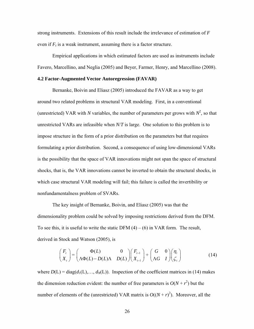
The key insight of Bernanke, Boivin, and Eliasz (2005) was that the

dimensionality problem could be solved by imposing restrictions derived from the DFM.

To see this, it is useful to write the static DFM (4) – (6) in VAR form. The result,

derived in Stock and Watson (2005), is

t

t

FX

⎛ ⎞⎜⎝ ⎠

⎟ = + ( ) 0

( ) ( ) ( )L

L D L D LΦ⎛ ⎞

⎜ ⎟ΛΦ − Λ⎝ ⎠1

1

t

t

FX

−

−

⎛ ⎞⎜ ⎟⎝ ⎠

0GG I

⎛ ⎞⎜ ⎟Λ⎝ ⎠

t

t

ηζ⎛ ⎞⎜ ⎟⎝ ⎠

(14)

where D(L) = diag(d1(L),…, dN(L)). Inspection of the coefficient matrices in (14) makes

the dimension reduction evident: the number of free parameters is O(N + r2) but the

number of elements of the (unrestricted) VAR matrix is O((N + r)2). Moreover, all the

26

parameters of (14) can be estimated by regressions involving Xt, , and the residuals

from the regression of Xt on

tF

tF . In particular, the (population) impulse response function

with respect to the innovations ηt is given by Γ(L) in Xt = Γ(L)ηt + et, where Γ(L) =

ΛΦ(L)−1G (this is obtained by substituting (5) into (4)). The factor loadings Λ can be

estimated by a regression of Xt on , the lag polynomial Φ(L) can be obtained from a

VAR estimated using , the matrix G can be estimated as the eigenvectors

corresponding to the q largest eigenvalues of the r×r variance matrix of the residuals

from the

tF

tF

tF VAR (in population this variance matrix has only q nonzero eigenvalues) ,

and ηt can be estimated by ˆtη = 1ˆ ˆˆ ( )t L F −G F t⎡ ⎤−Φ′⎣ ⎦ (for details see Stock and Watson

(2005)). This provides sample counterparts to the population innovations ηt, with an

arbitrary normalization, and to the impulse response function based on these innovations.

The SVAR modeling exercise now entails imposing sufficient identification

restrictions so that the structural shocks (or a single structural shock) can be identified as

a linear combination of ηt; that is, so that a q×q matrix R (or a row of R) can be identified

such that Rηt = εt, where εt are the q structural shocks. Forni, Giannone, Lippi, and

Reichlin (2009) show that, under plausible heterogeneity conditions on impulse response

functions, such a matrix R will in general exist and will be full rank, that is, the DFM

innovations will span the space of structural shocks so a FAVAR will solve the

invertibility problem. The matrix R (or individual rows of the matrix) can be identified

using extensions of the usual SVAR identification toolkit, including imposing short run

restrictions (see for example Bernanke, Boivin, and Eliasz (2005)); imposing long run

restrictions akin to those in Blanchard and Quah (1989) and King, Plosser, Stock, and

27

Watson (1991); identifying shocks by maximizing the fraction of the variance of common

components of one or more variables (Giannone, Reichlin, and Sala (2004)); and

imposing sign restrictions (Ahmadi and Uhlig (2009)).

4.3 DSGE estimation using DFMs

Sargent (1989) showed that the DFM can be interpreted as relating multiple

indicators to a latent low-dimensional model of the economy. Bovin and Giannoni

(2006) extend this concept by associating the dynamic factor evolution equation (2) with

a log-linearized DSGE. Accordingly, the elements of ft correspond to latent economic

concepts such as inflation and the output gap. The statistical agencies do not observe

these latent concepts, but instead produce multiple measures of them, for example

different rates of inflation derived from different price indexes. Similarly,

econometricians can produce multiple measures of the unobserved output gap. These

observable series constitute Xt, and the elements of ft are identified by exclusion

restrictions in the factor loadings (for example, the multiple observed measures of

inflation depend directly on the latent inflation factor but not on the other factors).

By introducing multiple indicators of these latent processes, Boivin and Giannoni

(2006) bring additional information to bear on the difficult task of estimation of DSGE

parameters. In principle this estimation could be done by MLE, however Boivin and

Giannoni (2006) use the Bayesian/Markov Chain Monte Carlo methods common in the

DSGE estimation literature.

28

5. Selected Extensions

This section briefly reviews three extensions of DFM research: DFMs with

breaks; DFMs that incorporate cointegration and error correction; and structured DFMs

such as hierarchical DFMs.

5.1 Breaks and time-varying parameters

Few papers have considered DFMs with breaks or time-varying parameters.

Stock and Watson (2002a) showed that the principal components estimator of the factors

is consistent even with certain types of breaks or time variation in the factor loadings.

The intuition for this result returns to the idea, introduced in Section 2.l, that the cross-

sectional averaging estimator is consistent for the space spanned by the factors

under relatively weak conditions on W, specifically N–1W′Λ → H; it stands to reason,

then, that Λ can break or evolve in some limited fashion and the principal components

estimator will remain consistent.

1ˆ (tF N W− )

Stock and Watson (2009a) considered the case of a single large break with one set

of factors and loadings before the break and another set after. They showed that the full-

sample principal components estimator of the factor asymptotically spans the space of the

two combined factors. Specifically, the factors for the pre-break subsample will be

estimated by one linear combination of the principal components, and the post-break

factors will be estimated by another linear combination. The break date need not be

known or estimated for this to hold. Accordingly, with a break, the number of full-

sample factors can exceed the number of subsample factors both before and after the

break. In an empirical application to U.S. macroeconomic data, they find that forecasts

29

based on full-sample factors can outperform those based on subsample factors, even

though a break is found empirically.

Breitung and Eickmeier (2009) propose a test for a single structural break in the

factor loadings at an unknown date in a DFM, in the ith equation of the static DFM (4).

For example, this can be done by regressing Xit on and interacted with the binary

variable that equals 1 for t > τ, (where τ is a hypothesized break date), then computing

the Wald statistic testing whether the coefficients on the interacted variables equal zero.

Breitung and Eickmeier (2009) find evidence of a change in the factor space in the U.S.

in the mid-1980s.

tF tF

Banerjee, Marcellino, and Masten (2007) provide Monte Carlo results on factor-

based forecasting with instability in the factor loadings, and find that large breaks, if

undetected, can substantially reduce the performance of full-sample factor-based

forecasts. This is consistent with the forecast function changing when the factor loadings

change, despite the space being spanned by the factors being consistently estimated. In

their setting, it is desirable to estimate the forecasting equation using the post-break

sample. They also report an application to data from the EU and from Slovenia, which

investigates split-sample instability in the factor forecasts (but not the factor estimates

themselves).

5.2 Incorporating cointegration and error correction

All the work discussed until now has assumed that all elements of Xt are

integrated of order 0 (I(0)). Typically this involves taking first differences of logarithms

for real variables, for example. Elements of Xt can also include other stationary

30

transformations, including error correction terms; for example it is common for interest

rate spreads to be included in Xt.

The econometric theory of principal components estimation of the factors requires

modification to cover integrated and cointegrated variables. The basic difficulty can be

seen by imagining that the original series are all independent random walks, so that Xt is a

vector of standardized independent random walks. These independent walks will be

subject to the spurious regression problem (Granger and Newbold (1974)) so without

further modification will have a limiting expression (as T → ∞, N fixed) in terms of a

N-dimensional demeaned Brownian motion, and

ˆXΣ

ˆXΣ will have many large eigenvalues

even though the elements of Xt are independent.

Some recent papers propose techniques designed to estimate and exploit factor

structure in the presence of nonstationary factors. Bai (2004) shows that if the factors are

I(1) and the idiosyncratic disturbances are I(0) – that is, if the Stock-Watson (1988)

common trends representation of cointegrated variables holds – then the space spanned

by the factors can be estimated consistently, as can the number of factors. Bai and Ng

(2004) provide a procedure for estimating the number of nonstationary factors even if

some of the idiosyncratic disturbances are integrated of order one (I(1)). Banerjee and

Marcellino (2008) use the common trends representation to introduce a factor error

correction model. Banerjee, Marcellino, and Masten (2009) provide empirical evidence

suggesting that forecasts based on the factor error correction model outperform standard

DFM forecasts. A premise of this research is that there is large-scale cointegration in the

levels variables or, equivalently, that the spectral density of the transformed variables (Xt

as defined for the previous sections) has a rank of only r << N at frequency zero.

31

5.3 Hierarchical DFMs

In certain specialized cases, hierarchical structures arise naturally and can be

incorporated into DFMs. Kose, Otrok, and Whiteman (2003) provide an early example

of such a model, in which both regional and global factors affect the evolution of output,

investment, and consumption in 60 countries. Ng and Moench (2009) provide an

application to regional housing prices and Stock and Watson (2010) provide a related

application to state-level housing starts. Moench, Ng, and Potter (2009) provide a

general formulation of multilevel hierarchical DFMs including extensive discussion of

computational issues.

5.4 Outlook

Dynamic factor models have the twin appeals of being grounded in dynamic

macroeconomic theory (Sargent (1989), Boivin and Giannoni (2006)) and providing a

good first-order description of empirical macroeconomic data, in the sense that a small

number of factors explain a large fraction of the variance of many macroeconomic series

(Sargent and Sims (1977), Giannone, Reichlin, and Sala (2004), Watson (2004)).

Theoretical econometric research on DFMs over the past decade has made a great deal of

progress, and a variety of methods are now available for the estimation of the factors and

of the number of factors. Theoretical work is ongoing in many related areas, including

weak factor structures, tests for the number of factors, and factor models with instability

and breaks.

The bulk of empirical work to date has focused on forecasting. A great deal is

now known about the performance of factor forecasts and about best practices for

forecasting using factors. Broadly speaking, this research has found that linear factor

32

forecasts perform well to very well relative to competitors for many, but not all,

macroeconomic series. For U.S. real activity series, reductions in pseudo out-of-sample

mean squared forecast errors at the two- to four-quarter horizon are often in the range of

20%-40%, although smaller or no improvements are seen for other series, such as U.S.

inflation post-1990. Parametric (third-generation) DFMs are also particularly well suited

for nowcasting. Work on other empirical applications of DFMs, such as structural VARs

and estimation of parameters of DSGEs, is newer and while there are relatively few such

applications to date, these constitute promising directions for future empirical research.

33

References

Ahmadi, P A., and H. Uhlig (2009), "Measuring the Effects of a Shock to Monetary

Policy: A Bayesian Factor-Augmented VAR Approach with Sign Restrictions”,

manuscript, University of Chicago.

Ahn, S.C. and A.R. Horenstein (2009), “Eigenvalue Ratio Test for the Number of

Factors,” manuscript, Arizona State University.

Amemiya, T. (1966), “On the Use of Principal Components of Independent Variables in

Two-Stage Least-Squares Estimation,” International Economic Review 7, 283-

303.

Amengual, D., and M.W. Watson (2007), “Consistent Estimation of the Number of

Dynamic Factors in a Large N and T Panel,” Journal of Business and Economic

Statistics, 91-96.

Anderson, T.W. (1984), An Introduction to Multivariate Statistical Analysis, second

edition, New York: Wiley.

Angelini, E., N. Bańbura, and G. Rünstler (2008), “Estimating and Forecasting the Euro

Area Monthly National Accounts from a Dynamic Factor Model,” ECB Working

Paper No. 593.

Aruoba, S.B., F.X. Diebold, and C. Scotti (2009), “Real-Time Measurement of Business

Conditions,” Journal of Business & Economic Statistics 27, 417-427.

Bai, J. (2003), “Inferential Theory for Factor Models of Large Dimensions,”

Econometrica, 71, 135-172.

Bai, J., and S. Ng (2002), “Determining the Number of Factors in Approximate Factor

Models,” Econometrica, 70, 191-221.

34

Bai, J., and S. Ng (2004), “A PANIC Attack on Unit Roots and Cointegration,”

Econometrica, 72, 1127-1177.

Bai, J., and S. Ng (2006a), “Confidence Intervals for Diffusion Index Forecasts and

Inference for Factor-Augmented Regressions,” Econometrica, 74,1133-1150.

Bai, J., and S. Ng (2006b), “Determining the Number of Factors in Approximate Factor

Models, errata” manuscript, Columbia University.

Bai, J., and S. Ng (2007), “Determining the Number of Primitive Shocks in Factor

Models,” Journal of Business and Economic Statistics 25, 52-60.

Bai, J., and S. Ng (2008), “Large Dimensional Factor Analysis,” Foundations and Trends

in Econometrics, 3(2): 89-163.

Bai, J. and S. Ng (2010), “Instrumental Variable Estimation in a Data-Rich

Environment,” Forthcoming, Econometric Theory

Banerjee, A., and M. Marcellino (2008) "Factor Augmented Error Correction Models",

CEPR WP 6707.

Banerjee, A., M. Marcellino, and I. Masten (2007), “Forecasting Macroeconomic

Variables Using Diffusion Indexes in Short Samples With Structural Change,”

forthcoming in Forecasting in the Presence of Structural Breaks and Model

Uncertainty, ed. by D. Rapach and M. Wohar, Elsevier.

Banerjee, A., M. Marcellino and I. Masten, (2009), Forecasting with Factor-augmented

Error Correction Models , mimeo, European University Institute

Bernanke, B.S., J. Boivin, and P. Eliasz (2005), “Measuring the Effects of Monetary

Policy: A Factor-Augmented Vector Autoregressive (FAVAR) Approach,”

Quarterly Journal of Economics, 120, 387-422.

35

Beyer A., Famer R., Henry J. and M. Marcellino (2008) "Factor Analysis in a New-

Keynesian Model,” Econometrics Journal, forthcoming

Blanchard, O.J., and D. Quah (1989), “Dynamic Effects of Aggregate Demand and

Supply Disturbances,” American Economic Review, 79, 655-673.

Boivin, J., and M. Giannoni (2006), “DSGE Models in a Data-Rich Environment,”

NBER Working Paper no. 12772.

Boivin, J., and S. Ng (2005), “Understanding and Comparing Factor-Based Forecasts,”

International Journal of Central Banking 1, 117-151.

Boivin J. and S. Ng (2006) "Are More Data Always Better for Factor Analysis?",

Journal of Econometrics, 132, p. 169-194.

Brillinger, D.R. (1964), “A Frequency Approach to the Techniques of Principal

Components, Factor Analysis and Canonical Variates In the Case of Stationary

Time Series,” Invited Paper, Royal Statistical Society Conference, Cardiff Wales.

(Available at http://stat-www.berkeley.edu/users/brill/ papers.html).

Brillinger, D.R. (1981), Time Series: Data Analysis and Theory, expanded edition, San

Francisco: Holden-Day.

Breitung, J. and S. Eickmeier (2009), “Testing for Structural Breaks in Dynamic Factor

Models,” Deutsche Bundesbank Economic Studies Discussion Paper No.

05/2009.

Carlin, B.P., N.G. Polson, and D.S. Stoffer (1992), “A Monte Carlo Approach to

Nonnormal and Nonlinear State-Space Modeling,” Journal of the American

Statistical Association, 87, 493-500.

36

Cattell, R. B. (1966) “The Scree Test for the Number of Factors”, Multivariate

Behavioral Research, vol. 1, 245-76.

Chamberlain, G., and M. Rothschild (1983), “Arbitrage Factor Structure, and Mean-

Variance Analysis of Large Asset Markets,” Econometrica, 51,1281-1304.

Chib, S. and E. Greenberg (1996), “Markov Chain Monte Carlo Simulation Methods in

Econometrics,” Econometric Theory, 12, 409-431.

Connor, G., and R.A. Korajczyk (1986), “Performance Measurement with the Arbitrage

Pricing Theory,” Journal of Financial Economics, 15, 373-394.

D’Agostino, A., and Domenico Giannone (2006), “Comparing Alternative Predictors

Based on Large-Panel Factor Models,” ECB Working Paper 680.

Doz, C., D. Giannone, and L. Reichlin (2006), “A Quasi Maximum Likelihood Approach

for Large Approximate Dynamic Factor Models,” ECB Working Paper 674.

Eickmeier, S., C. Ziegler (2008), How successful are dynamic factor models at

forecasting output and inflation? A meta-analytic approach, Journal of

Forecasting, 27(3), 237-265.

El Karoui, N. (2007), “Tracy-Widom Limit for the Largest Eigenvalue of a Large Class

of Complex Sample Covariance Matrices,” Annals of Probability, 35, 633-714.

Engle, R.F., and M.W. Watson (1981), “A One-Factor Multivariate Time Series Model of

Metropolitan Wage Rates,” Journal of the American Statistical Association, 76,

774-781.

Engle, R.F., and M.W. Watson (1983), “Alternative Algorithms for Estimation of

Dynamic MIMIC, Factor, and Time Varying Coefficient Regression Models,”

Journal of Econometrics, Vol. 23, pp. 385-400.

37

Favero, C.A., M. Marcellino, and F. Neglia (2005), “Principal Components at Work: The

Empirical Analysis of Monetary Policy With Large Datasets,” forthcoming,

Journal of Applied Econometrics.

Forni, M., D. Giannone, M. Lippi, and L. Reichlin (2009), “Opening the Black Box:

Structural Factor Models with Large Cross Sections,” Econometric Theory, 25,

1319-1347.

Forni, M., M. Hallin, M. Lippi, and L. Reichlin (2000), “The Generalized Factor Model:

Identification And Estimation,” Review of Economics and Statistics, 82, 540–554.

Forni, M., M. Hallin, M. Lippi, and L. Reichlin (2004), “The Generalized Factor Model:

Consistency and Rates,” Journal of Econometrics, 119, 231-255.

Forni, M., M. Hallin, M. Lippi, and L. Reichlin (2005), “The Generalized Dynamic

Factor Model: One-Sided Estimation and Forecasting,” Journal of the American

Statistical Association, 100, 830-839.

Forni, M., and L. Reichlin (1998), “Let’s Get Real: A Dynamic Factor Analytical

Approach to Disaggregated Business Cycle,” Review of Economic Studies, 65,

453-474.

Geweke, J. (1977), “The Dynamic Factor Analysis of Economic Time Series,” in Latent

Variables in Socio-Economic Models, ed. by D.J. Aigner and A.S. Goldberger,

Amsterdam: North-Holland.

Geweke, J. and R. Meese (1981), “Estimating Regression Models of Finite but Unknown

Order,” International Economic Review 22, no. 1, 55-70.

Giannone, D., L. Reichlin, and L. Sala (2004), “Monetary Policy in Real Time,” NBER

Macroeconomics Annual, 2004, 161-200.

38

Giannone, D., L. Reichlin, and D. Small (2008), “Nowcasting: The Real-Time

Informational Content of Macroeconomic Data,” Journal of Monetary Economics,

55, 665-676.

Granger, P. and C.W.J. Newbold (1974), “Spurious Regressions in Econometrics,”

Journal of Econometrics 2, 111-120.

Hallin, M., and Liška, R., (2007), “The Generalized Dynamic Factor Model: Determining

the Number of Factors,” Journal of the American Statistical Association, 102,

603-617.

Hamilton, J.D., (1989), “A New Approach to the Economic Analysis of Nonstationary

Time Series and the Business Cycle,” Econometrica, 57, 357-384.

Harvey, A.C. (1989), Forecasting, Structural Time Series Models and the Kalman Filter.

Cambridge, U.K.: Cambridge University Press, 1989

Johnstone, I.M. (2001), “On the Distribution of the Largest Eigenvalue in Principal

Component Analysis,” Annals of Statistics, 29, 295-327.

Jungbacker, D., and S.J. Koopman (2008), “Likelihood-Based Analysis for Dynamic

Factor Models,” manuscript, Tinbergen Institute.

Jungbacker, D., S.J. Koopman, and M. van der Wel (2009), “Dynamic Factor Analysis in

the Presence of Missing Data,” Tinbergen Institute Discussion Paper 2009-010/4.

Kapetanios, G., and M. Marcellino (2008), “Factor-GMM Estimation with Large Sets of

Possibly Weak Instruments,” manuscript, EUI

Kim, C-J., and C. Nelson (1998), “Business Cycle Turning Points, A New Coincident

Index, and Tests of Duration Dependence Based on a Dynamic Factor Model with

Regime-Switching,” Review of Economics and Statistics, 80(2), 188-201.

39

King, Robert G., C.I. Plosser, J.H. Stock, and M.W. Watson (1991), “Stochastic Trends

and Economic Fluctuations,” American Economic Review 81(4): 819-840.

Kitagawa, G., (1987), “Non-Gaussian State Space Modeling of Non-Stationary Time

Series,” with discussion, Journal of the American Statistical Association, 82,

1032-1063.

Kloek, T., and L.B.M. Mennes (1960), “Simultaneous Equations Estimation Based on

Principal Components of Predetermined Variables,” Econometrica, 28, 45-61.

Kose, A., C. Otrok, C., and C. Whiteman, (2003), “International Business Cycles: World

Region and Country Specific Factors,” American Economic Review 93:4, 1216-

1239.

Kose, A., C. Otrok, C., and C. Whiteman, (2008), “Understanding the Evolution of

World Business Cycles,” Journal of International Economics, 75, 110-130.

Marcellino, M., J.H. Stock, and M.W. Watson, (2006), “A Comparison of Direct and

Iterated Multistep AR Methods for Forecasting Macroeconomic Series,” Journal

of Econometrics, 135, 499-526.

Moench E. and S. Ng and S. Potter (2009), “Dynamic Hierarchical Factor Models,”

manuscript, Columbia University.

Ng, S. and E. Moench (2009), “A Factor Analysis of Housing Market Dynamics in the

U.S. and the Regions,” manuscript, Columbia University.

Onatski, A. (2008), “The Tracy-Widom Limit for the Largest Eigenvalues of Singular

Complex Wishart Matrices,” Annals of Applied Probability 18, 470-490.

Onatski, Alexei (2009), “Testing Hypotheses about the Number of Factors in Large

Factor Models,” Econometrica 77 1447-1479.

40

Otrok, C., and C.H. Whiteman, (1998), “Bayesian Leading Indicators: Measuring and

Predicting Economic Conditions in Iowa,” International Economic Review, 39(4).

Quah, D., and T.J. Sargent (1993), “A Dynamic Index Model for Large Cross Sections”

(with discussion), in Business Cycles, Indicators, and Forecasting, ed. by J.H.

Stock and M.W. Watson, Chicago: University of Chicago Press for the NBER,

285-310.

Reiss, R., and M.W. Watson (2010), “Relative Goods’ Prices and Pure Inflation,”

American Economic Journal: Macroeconomics, forthcoming.

Sargent, T.J. (1989), “Two Models of Measurements and the Investment Accelerator,”

Journal of Political Economy 97:251–287.

Sargent, T.J., and C.A. Sims (1977), “Business Cycle Modeling Without Pretending to

Have Too Much A-Priori Economic Theory,” in New Methods in Business Cycle

Research, ed. by C. Sims et al., Minneapolis: Federal Reserve Bank of

Minneapolis.

Stock, J.H. and M.W. Watson (1988), “Testing for Common Trends,” Journal of the

American Statistical Association 83, no. 404, 1097-1107.

Stock, J.H., and M.W. Watson (1989), “New Indexes of Coincident and Leading

Economic Indicators,” NBER Macroeconomics Annual 1989, 351-393.

Stock, J.H., and M.W. Watson (1999), “Forecasting Inflation,” Journal of Monetary

Economics, 44, 293-335.

Stock, J.H., and M.W. Watson (2002a), “Forecasting Using Principal Components from a

Large Number of Predictors,” Journal of the American Statistical Association, 97,

1167-1179.

41

Stock, J.H., and M.W. Watson (2002b), “Macroeconomic Forecasting Using Diffusion

Indexes,” Journal of Business and Economic Statistics, 20, 147-162.

Stock, J.H., and M.W. Watson (2005), “Implications of Dynamic Factor Models for VAR

Analysis,” manuscript.

Stock, J.H., and M.W. Watson (2006), “Forecasting with Many Predictors,” ch. 6 in

Handbook of Economic Forecasting, ed. by Graham Elliott, Clive W.J. Granger,

and Allan Timmermann, Elsevier, 515-554.

Stock, J.H., and M.W. Watson (2009a), “Forecasting in Dynamic Factor Models Subject

to Structural Instability,” Ch. 7. in Neil Shephard and Jennifer Castle (eds), The

Methodology and Practice of Econometrics: Festschrift in Honor of D.F. Hendry.

Oxford; Oxford University Press.

Stock, J.H., and M.W. Watson (2009b), “Phillips Curve Inflation Forecasts,” Ch. 3 in

Understanding Inflation and the Implications for Monetary Policy (2009), Jeffrey

Fuhrer, Yolanda Kodrzycki, Jane Little, and Giovanni Olivei (eds). Cambridge:

MIT Press.

Stock, J.H., and M.W. Watson (2009c), “Generalized Shrinkage Methods for Forecasting

Using Many Predictors,” manuscript.

Stock, J.H., and M.W. Watson (2010), “The Evolution of National and Regional Factors

in U.S. Housing Construction,” Ch. 3 in T. Bollerslev, J. Russell, and M. Watson

(eds), Volatility and Time Series Econometrics: Essays in Honor of Robert F.

Engle, Oxford; Oxford University Press.

Tracy, C.A., and H. Widom (1994), “Level Spacing Distributions and the Airy Kernel,”

Communications in Mathematical Physics, 159, 151-174.

42

43

Watson, M.W. (2004), “Comment on Giannone, Reichlin, and Sala,” NBER

Macroeconomics Annual, 2004, 216-221.