dynamic equicorrelation journal of business & economic...

This article was downloaded by: [University of Chicago]On: 28 July 2012, At: 03:11Publisher: Taylor & FrancisInforma Ltd Registered in England and Wales Registered Number: 1072954 Registered office: Mortimer House,37-41 Mortimer Street, London W1T 3JH, UK

Journal of Business & Economic StatisticsPublication details, including instructions for authors and subscription information:http://amstat.tandfonline.com/loi/ubes20

Dynamic EquicorrelationRobert Engle a & Bryan Kelly ba Stern School of Business, New York University, 44 W. 4th St. Suite 9-190, New York, NY,10012b Booth School of Business, University of Chicago, 5807 S. Woodlawn Ave., Chicago, IL, 60637

Accepted author version posted online: 12 Jan 2012. Version of record first published: 24May 2012

To cite this article: Robert Engle & Bryan Kelly (2012): Dynamic Equicorrelation, Journal of Business & Economic Statistics,30:2, 212-228

To link to this article: http://dx.doi.org/10.1080/07350015.2011.652048

PLEASE SCROLL DOWN FOR ARTICLE

Full terms and conditions of use: http://amstat.tandfonline.com/page/terms-and-conditions

This article may be used for research, teaching, and private study purposes. Any substantial or systematicreproduction, redistribution, reselling, loan, sub-licensing, systematic supply, or distribution in any form toanyone is expressly forbidden.

The publisher does not give any warranty express or implied or make any representation that the contentswill be complete or accurate or up to date. The accuracy of any instructions, formulae, and drug doses shouldbe independently verified with primary sources. The publisher shall not be liable for any loss, actions, claims,proceedings, demand, or costs or damages whatsoever or howsoever caused arising directly or indirectly inconnection with or arising out of the use of this material.

http://amstat.tandfonline.com/loi/ubes20

http://dx.doi.org/10.1080/07350015.2011.652048

http://amstat.tandfonline.com/page/terms-and-conditions

Supplementary materials for this article are available online. Please go to http://tandfonline.com/r/JBES

Dynamic Equicorrelation

Robert ENGLEStern School of Business, New York University, 44 W. 4th St. Suite 9-190, New York, NY 10012([email protected])

Bryan KELLYBooth School of Business, University of Chicago, 5807 S. Woodlawn Ave., Chicago, IL 60637([email protected])

A new covariance matrix estimator is proposed under the assumption that at every time period all pairwisecorrelations are equal. This assumption, which is pragmatically applied in various areas of finance, makes itpossible to estimate arbitrarily large covariance matrices with ease. The model, called DECO, involves firstadjusting for individual volatilities and then estimating correlations. A quasi-maximum likelihood resultshows that DECO provides consistent parameter estimates even when the equicorrelation assumption isviolated. We demonstrate how to generalize DECO to block equicorrelation structures. DECO estimatesfor U.S. stock return data show that (block) equicorrelated models can provide a better fit of the data thanDCC. Using out-of-sample forecasts, DECO and Block DECO are shown to improve portfolio selectioncompared to an unrestricted dynamic correlation structure.

KEY WORDS: Conditional covariance; Dynamic conditional correlation; Equicorrelation; MultivariateGARCH.

1. INTRODUCTION

Since the first volatility models were formulated in the early1980s, there have been efforts to estimate multivariate models.The specifications of these models were developed over the past25 years with a range of papers surveyed by Bollerslev, Engle,and Nelson (1994) and more recently by Bauwens, Laurent, andRombouts (2006) and Silvennoinen and Terasvirta (2008). Ageneral conclusion from this analysis is that it is difficult to esti-mate multivariate GARCH models with more than half a dozenreturn series because the specifications are so complicated.

Recently, Engle (2002) proposed Dynamic Conditional Cor-relation (DCC), greatly simplifying multivariate specifications.DCC is designed for high-dimensional systems but has onlybeen successfully applied to up to 100 assets by Engle andSheppard (2005). As the size of the system grows, estimationbecomes increasingly cumbersome. For cross-sections of hun-dreds or thousands of stocks, as are common in asset pricingapplications, estimation can break down completely.

Approaches exist to address the high-dimension problem,though each has limitations. One type of approach is to im-pose structure on the system such as a factor model. UnivariateGARCH dynamics in factors can generate time-varying corre-lations while keeping the residual correlation matrix constantthrough time. This idea motivated the Factor ARCH models ofEngle, Ng, and Rothschild (1990, 1992) and Engle’s (2009b)Factor Double ARCH. The benefit of these models is their fea-sibility for large numbers of variates: If there are n dependentvariables and k factors, estimation requires only n + k GARCHmodels. Furthermore, it uses a full likelihood and will be ef-ficient under appropriate conditions. One drawback is that itis not always clear what the factors are, or factor data maynot be available. Another is that correlation dynamics can ex-ist in residuals even after controlling for the factors, as in thecase of U.S. equity returns (Engle 2009a,b; Engle and Rangel2012). Addressing either of these problems leads back to the

unrestricted DCC specification, and thus to the dimensionalitydilemma.

A second solution uses the method of composite likelihood.This method was recently proposed by Engle, Shephard, andSheppard (2008) to estimate unrestricted DCC for vast cross-sections. Composite likelihood overcomes the dimension limi-tation by breaking a large system into many smaller subsystemsin a way that generalizes the “MacGyver” method of Engle(2009a,b). This approach possesses great flexibility, but willgenerally be inefficient due to its reliance on a partial likelihood.

The contrast of Factor ARCH and composite likelihood high-lights a fundamental tradeoff in large-system conditional covari-ance modeling. Imposing structure on the covariance can makeestimation feasible and, if correctly specified, efficient; but itsacrifices generality and can suffer from breakdowns due tomisspecification. On the other hand, less structured models likecomposite likelihood break the curse of dimensionality whilemaintaining a general specification. However, its cost is a lossof efficiency from using a partial likelihood.

We propose a solution to this tradeoff that selectively com-bines simplifying structural assumptions and composite like-lihood versatility. We consider a system in which all pairs ofreturns have the same correlation on a given day, but this corre-lation varies over time. The model, called Dynamic Equicorre-lation (DECO), eliminates the computational and presentationaldifficulties of high-dimension systems. Because equicorrelatedmatrices have simple analytic inverses and determinants, like-lihood calculation is dramatically simplified and optimizationbecomes feasible for vast numbers of assets.

DECO’s structure can be substantially weakened by us-ing block equicorrelated matrices, while maintaining the

© 2012 American Statistical AssociationJournal of Business & Economic Statistics

April 2012, Vol. 30, No. 2DOI: 10.1080/07350015.2011.652048

212

Dow

nloa

ded

by [

Uni

vers

ity o

f C

hica

go]

at 0

3:11

28

July

201

2

http://www.tandfonline.com/r/JBES

mailto:[email protected]

mailto:[email protected]

http://www.amstat.org

http://pubs.amstat.org/loi/jbes

http://dx.doi.org/10.1080/07350015.2011.652048

Engle and Kelly: Dynamic Equicorrelation 213

simplicity and robustness of the basic DECO formulation. Ablock model may capture, for instance, industry correlationstructures. All stocks within an industry share the same correla-tion while correlations between industries take another value. Inthe two-block setting, analytic inverses and determinants are stillavailable and fairly simple, thus optimization for the two-BlockDECO model is as easy as the one-block case. The two-blockstructure can also be combined with the method of compositelikelihood to estimate Block DECO with an arbitrary numberof blocks. Since the subsets of assets used in Block DECO arepairs of blocks rather than pairs of assets, a larger portion ofthe likelihood (and therefore more information) is used for op-timization. As a result, the estimator can be more efficient thanunrestricted composite likelihood DCC.

Another way to enrich dependence beyond equicorrelation isto combine DECO with Factor (Double) ARCH. To understandhow this may work, consider a model in which one factor isobservable and the dispersion of loadings on this factor is high.Further, suppose each asset loads roughly the same on a second,latent, factor. The first factor contributes to diversity amongpairwise correlations, and is clearly not driven by noise. Thus,DECO may be a poor candidate for describing raw returns.However, residuals from a regression of returns on only the firstfactor will be well described by DECO. One way to model thisdataset is to use Factor Double ARCH with DECO residuals.Such a model is estimated by first using GARCH regressionmodels for each stock, then applying DECO to the standardizedresiduals.

What will occur if DECO is applied to variables that are notequicorrelated? If (block) equicorrelation is violated, DECO canstill provide consistent parameter estimates. In particular, weprove quasi-maximum likelihood results showing that if DCCis a consistent estimator, then DECO and Block DECO willbe consistent also. This means that when the true model isDCC, DECO makes estimation feasible when the dimensionof the system may be otherwise too large for DCC to handle.While DECO is closely related to DCC, the two models arenonnested: DECO is not simply a restricted version of DCC,but a competing model. Indeed, DECO possesses some subtle,though important, features lacking in DCC. A key example isthat DECO correlations between any pair of assets i and j dependon the return histories of all pairs. For the analogous DCCspecification (i.e., using the same number of parameters), thei, j correlation depends on the histories of i and j alone. In thissense, DECO parsimoniously draws on a broader informationset when formulating the correlation process of each pair. Tothe extent that true correlations are affected by realizations ofall assets, the failure of DCC to capture the information poolingaspect of DECO can disadvantage DCC as a descriptor of thedata-generating process.

In a one-factor world, the relation between the return on anasset and the market return is

rj = βj rm + ej , σ 2j = β2

j σ2m + vj .

If the cross-sectional dispersion of βj is small and idiosyncrasieshave similar variance over each period, then the system is well-described by Dynamic Equicorrelation. A natural application forthis one-factor structure lies in the market for credit derivativessuch as collateralized debt obligations, or CDOs. A key featureof the risk in loan portfolios is the degree of correlation be-

tween default probabilities. A simple industry valuation modelallows this correlation to be one number if firms are in the sameindustry and a different and smaller number if they are in differ-ent industries. Hence, within each industry, an equicorrelationassumption is being made.

More broadly, to price CDOs, an assumption is often madethat these are large homogeneous portfolios (LHPs) of corporatedebt. As a consequence, each asset will have the same variance,the same covariance with the market factor, and the same id-iosyncratic variance. Thus, in an LHP, the j subscripts disappear.The correlation between any pair of assets then becomes

ρ = β2σ 2m

β2σ 2m + v

.

In fact, the LHP assumption implies equicorrelation.The equicorrelation assumption also surfaces in derivatives

trading. For instance, a popular position is to buy an option ona basket of assets and then sell options on each of the compo-nents, sometimes called a dispersion trade. By delta hedgingeach option, the value of this position depends solely on the cor-relations. Let the basket have weights given by the vector w, andlet the implied covariance matrix of components of the basketbe given by the matrix S. Then, the variance of the basket can beexpressed as σ 2 = w′Sw. In general, we only know about thevariances of implied distributions, not the covariances. Hence,it is common to assume that all correlations are equal, givingσ 2 = ∑n

j=1 w2j s

2j + ρ

∑i �=j wiwj sisj , which can be solved for

the implied correlation

ρ = σ 2 −∑nj=1 w2

j s2j∑

i �=j wiwj sisj

. (1)

As a consequence, the value of this position depends upon theevolution of the implied correlation. When each of the variancesis a variance swap made up of a portfolio of options, the fullposition is called a correlation swap. As the implied correlationrises, the value of the basket variance swap rises relative to thecomponent variance swaps.

There is substantial history of the use of equicorrelation ineconomics. In early studies of asset allocation, Elton and Gru-ber (1973) found that assuming all pairs of assets had the samecorrelation reduced estimation noise and provided superior port-folio allocations over a wide range of alternative assumptions.Berndt and Savin (1975) studied what could be called equiauto-correlation matrices in production factor and consumer demandsystems as a means of working with singular error variancematrices. Ledoit and Wolf (2004) used Bayesian methods forshrinking the sample correlation matrix to an equicorrelatedtarget and showed that this helps select portfolios with lowvolatility compared to those based on the sample correlation.Further prescriptions for avoiding the notorious noisiness of un-restricted sample correlations and betas abound in the literature(Ledoit and Wolf 2003, 2004; Michaud 1989; Jagannathan andMa 2003; Jobson and Korkie 1980; and Meng, Hu, and Bai 2011,among others). Ledoit and Wolf’s Bayesian shrinkage and Eltonand Gruber’s parameter averaging are different approaches tonoise reduction in unconditional correlation estimation. Whilethe Bayesian method has not yet been employed for conditionalvariances, DECO makes it possible to incorporate Elton andGruber’s noise reduction technique into a dynamic setting. By

Dow

nloa

ded

by [

Uni

vers

ity o

f C

hica

go]

at 0

3:11

28

July

201

2

214 Journal of Business & Economic Statistics, April 2012

averaging pairwise correlations, (Block) DECO smooths cor-relation estimates within groups. As long as this reduces es-timation noise more than it compromises the true correlationstructure, smoothing can be beneficial. Our empirical resultssuggest that the benefits of smoothing indeed extend to the con-ditional case. Across a range of first-stage factor models, (Block)DECO selects out-of-sample portfolios that have significantlylower volatilities than those chosen by unrestricted DCC.

The next section develops the DECO model and its theo-retical properties. Section 3 presents Monte Carlo experimentsthat assess the model’s performance under equicorrelated andnonequicorrelated generating processes. In Section 4, we ap-ply DECO, Block DECO, and DCC models to U.S. stock returndata. We find that DCC correlations between pairs of stocks havea large degree of comovement, suggesting that DECO may bebeneficial in describing the system’s correlation. Indeed, we findthat basic DECO, and DECO with 10 industry blocks, providea better fit of the data than DCC. Finally, we analyze the abil-ity of (Block) DECO to construct optimal out-of-sample hedgeportfolios. We find that (Block) DECO is the model that mostoften delivers MV portfolios with the lowest sample variance.

2. THE DYNAMIC EQUICORRELATION MODEL

We begin by defining an equicorrelation matrix and presenta result for its invertibility and positive definiteness that will beuseful throughout the article.

Definition 2.1 A matrix Rt is an equicorrelation matrix ofan n × 1 vector of random variables if it is positive definite andtakes the form

Rt = (1 − ρt )In + ρt Jn, (2)

where ρt is the equicorrelation, In denotes the n-dimensionalidentity matrix, and Jn is the n × n matrix of ones.

Lemma 2.1 The inverse and determinant of the equicorrela-tion matrix, Rt , are given by

R−1t = 1

1 − ρt

In + − ρt

(1 − ρt )(1 + [n − 1]ρt )Jn, (3)

and

det(Rt ) = (1 − ρt )n−1(1 + [n − 1]ρt ). (4)

Further, R−1t exists if and only if ρt �= 1 and ρt �= −1

n−1 , and Rt

is positive definite if and only if ρt ∈ ( −1n−1 , 1).

Proofs are provided in the online appendix.

Definition 2.2 A time series of n × 1 vectors {r̃ t } obeysa Dynamic Equicorrelation (DECO) model if vart−1(r̃ t ) =Dt Rt Dt , where Rt is given by Equation (2) for all t and Dt

is the diagonal matrix of conditional standard deviations of r̃ t .The dynamic equicorrelation is ρt .

2.1 Estimation

Like many covariance models, a two-stage quasi-maximumlikelihood (QML) estimator of DECO will be consistent andasymptotically normal under broad conditions including manyforms of model misspecification. We provide asymptotic results

here for a general framework that includes several standard mul-tivariate GARCH models as special cases, including DECO andthe original DCC model. The development is a slightly mod-ified reproduction of the two-step QML asymptotics of White(1994). After presenting the general result, we elaborate on prac-tical estimation of DECO using Gaussian returns and GARCHcovariance evolution.

First, define the (scaled) log quasi-likelihood of the model asL({r̃ t }, θ ,φ) = 1

T

∑Tt=1 log ft (r̃ t , θ ,φ), which is parameterized

by vector γ = (θ,φ) ∈ � = � × �. The two-step estimationproblem may be written as

maxθ∈�

L1({r̃ t }, θ ) = 1

T

T∑t=1

log f1,t (r̃ t , θ ), (5)

maxφ∈�

L2({r̃ t }, θ̂ ,φ) = 1

T

T∑t=1

log f2,t (r̃ t , θ̂ ,φ), (6)

where θ̂ is the solution to (5). The full two-stage QML estimatorfor this problem is γ̂ = (θ̂ , φ̂), where φ̂ is the second-stagemaximizer solving (6) given θ̂ . Under the technical assumptionslisted in the online appendix, White (1994) proves the followingresult for consistency and asymptotic normality of γ̂ .

Conjecture 2.1 (White 1994, theorem 6.11) Under Assump-tions B.1 through B.6 in the online appendix,

√T (γ̂ − γ ∗)

A∼ N (0, A∗−1 B∗ A∗−1),

where

A∗ =( ∇θθE[L1(r̃ t , θ

∗)] 0

∇θφE[L2(r̃ t , θ∗,φ∗)] ∇φφE[L2(r̃ t , θ

∗,φ∗)]

)and

B∗ = var

(T −1/2

∑t

(s∗1,t

′, s∗

2,t′)

),

where s∗1,t = ∇θL1(r̃ t , θ

∗) and s∗2,t = ∇φL2(r̃ t , θ

∗,φ∗).

In the remainder of the section, we assume that both DECOand DCC log densities and their derivatives satisfy AssumptionsB.1–B.4 and B.6 of Conjecture 2.1. These are high-level as-sumptions about continuity, differentiability, boundedness, andthe applicability of central limit theorems. Further, we assumethat the DCC model is identified, and this takes the form ofAssumption B.5. Note that we have not verified these assump-tions for the generating processes that we consider in this article.The dynamic covariance literature uniformly appeals to QMLasymptotic theory when performing inference, though satisfac-tion of high-level assumptions has not been established for anymodel that has been proposed in this area. A rigorous analysis ofasymptotic theory for multivariate GARCH processes remainsan important unanswered question. For this reason, we refer toany result that follows immediately from White’s (1994) Theo-rem 6.11 as a conjecture. We refer readers to the online appendixfor more detail on this point, as well as simulation evidence thatsupports the satisfaction of these high-level assumptions for theDECO model.

DECO is adopted for individual applications by specifying aconditional volatility model (i.e., defining the process for Dt )and a ρt process. We assume that each conditional volatility fol-lows a GARCH model. We work with volatility-standardized

Dow

nloa

ded

by [

Uni

vers

ity o

f C

hica

go]

at 0

3:11

28

July

201

2


returns, denoted by omitting the tilde, r t = D−1t r̃ t , so that

vart−1(r t ) = Rt .The basic ρt specification we consider derives from the DCC

model of Engle (2002) and its cDCC modification proposed byAielli (2009). The correlation matrix of standardized returns,RDCC

t , is given by

Qt = Q̄(1 − α − β) + α Q̃12t−1r t−1r ′

t−1 Q̃12t−1 + β Qt−1, (7)

RDCCt = Q̃

− 12

t Qt Q̃− 1

2t , (8)

where Q̃t replaces the off-diagonal elements of Qt with ze-ros but retains its main diagonal and Q̄ is the unconditionalcovariance matrix of standardized residuals.

DECO sets ρt equal to the average pairwise DCC correlation

RDECOt = (1 − ρt )In + ρt Jn×n, (9)

ρt = 1

n(n − 1)

(ι′ RDCC

t ι − n)= 2

n(n − 1)

∑i>j

qi,j,t√qi,i,t qj,j,t

,

(10)

where qi,j,t is the i, j th element of Qt . The following assump-tion and lemma ensure that DECO possesses certain propertiesimportant for dynamic correlation models.

Assumption 2.1 The matrix Q̄ is positive definite, α + β < 1,α > 0, and β > 0.

Lemma 2.2 Under Assumption 2.1, the correlation matricesgenerated by every realization of a DECO process according toEquations (7) through (10) are positive definite and the processis mean reverting.

The result states that, for any correlation matrix, the trans-formation to equicorrelation shown in Equations (9) and (10)results in a positive-definite matrix. The bounds ( −1

n−1 , 1) for ρt

are not assumptions of the model, but are guaranteed by thistransformation as long as RDCC

t is positive definite. As will beseen in our later discussion of Block DECO, bounds on permis-sible correlation values become looser as the number of blocksincreases.

We estimate DECO with Gaussian quasi-maximum likeli-hood, which embeds it in the framework of Conjecture 2.1. Con-ditional on past realizations, the return distribution is r̃ t |t−1 ∼N (0, H t ), H t = Dt Rt Dt . To establish notation, we use super-scripted densities f DECO

t and f DCCt to indicate the Gaussian den-

sity of r̃ t |t−1 assuming the covariance specifically obeys DECOor DCC, respectively. Similarly, superscripted log-likelihoodsLDECO and LDCC represent the log-likelihood of DECO or DCC.Omission of superscripts will be used to discuss densities andlog-likelihoods without specific assumptions on the dynamicsor structure of covariance matrices.

The multivariate Gaussian log-likelihood function L can bedecomposed (suppressing constants) as

L = 1

T

∑t

log(ft )

= − 1

T

∑t

(log |H t | + r̃ ′

t H−1t r̃ t

)

= − 1

T

∑t

(log |Dt |2 + r̃ ′

t D−2t r̃ t − r ′

t r t

)

− 1

T

∑t

(log |Rt | + r ′

t R−1t r t

).

Let θ ∈ � and φ ∈ � denote the vector of univariate volatilityparameters and the vector of correlation parameters, respec-tively. The above equation says that the log-likelihood can beseparated additively into two terms. The first term, which wecall L(θ), depends on the parameters of the univariate GARCHprocesses which affect only the Dt matrices and are indepen-dent of Rt and φ. The second term, which we call LCorr(θ,φ),depends on both the univariate GARCH parameters (embeddedin the r t terms) as well as the correlation parameters. Engle(2002) and Engle and Sheppard (2005) noted that correlationmodels of this form satisfy the assumptions of Conjecture 2.1.In particular, LVol(θ ) corresponds to L1 in the conjecture and θ̂

is the vector of first-stage volatility parameter estimates. L(θ̂,φ)corresponds to the second-step likelihood, L2, so φ̂ is the maxi-mizer of LCorr(θ̂,φ). Note that the model ensures stationarity andthat the covariance matrix remains positive definite in all peri-ods whenever Assumption 2.1 holds and the univariate GARCHmodels are stationary.

The vector γ̂ DECO is the two-stage Gaussian estimator whenthe second-stage likelihood obeys DECO. It assumes returns areGaussian and the correlation process obeys Equations (9) and(10). The following conjectures specifically apply Conjecture2.1 to the Gaussian DECO and DCC models.

Conjecture 2.2 Assuming that f DECOt and LDECO satisfy As-

sumptions B.1–B.6 with corresponding unique maximizer γ ∗,then γ̂ DECO is consistent and asymptotically normal for γ ∗.

The analogous corollary for γ̂ DCC, the two-stage GaussianDCC estimator, will be useful in developing our later compari-son between DECO and DCC.

Conjecture 2.3 Assuming that f DCCt and LDCC satisfy As-

sumptions B.1–B.6 with corresponding unique maximizer γ ∗,then γ̂ DCC is consistent and asymptotically normal for γ ∗.

In addition, the asymptotic covariance matrices for γ̂ DECO

and γ̂ DCC corresponding to Conjectures 2.2 and 2.3 take theform stated in Conjecture 2.1, replacing L1 and L2 with theappropriately superscripted likelihoods L

(·)Vol and L

(·)Corr.

To appreciate the payoff from making the equicorrelationassumption, consider the second step likelihood under DECO

LDECOCorr (θ̂,φ)

= − 1

T

∑t

(log |RDECO

t | + r̂ ′t RDECO

t

−1r̂ t

)

= − 1

T

∑t

[log

([1 − ρt ]

n−1[1 + (n − 1)ρt ]

)

+ 1

1 − ρt

(∑i

(r̂2i,t

)− ρt

1 + (n − 1)ρt

(∑i

r̂i,t

)2)],

where r̂ t are returns standardized for first-stage volatility esti-mates, r̂ t = Dt (θ̂ )−1 r̃ t , and ρt obeys Equation (10). In DCC,

Dow

nloa

ded

by [

Uni

vers

ity o

f C

hica

go]

at 0

3:11

28

July

201

2


the conditional correlation matrices must be recorded and in-verted for all t and their determinants calculated; further, theseT inversions and determinant calculations are repeated for eachof the many iterations required in a numeric optimization pro-gram. This is costly for small cross-sections and potentiallyinfeasible for very large ones. In contrast, DECO reduces com-putation to n-dimensional vector outer products with no matrixinversions or determinants required, rendering the likelihoodoptimization problem manageable even for vast-dimensionalsystems. The likelihood at time t can be calculated from justthree statistics, the average cross-sectional standardized return,the average cross-sectional squared standardized return, and thepredicted correlation. This is a simple calculation in all settingsconsidered in this article.

2.2 Differences Between DECO and DCC

The transformation from DCC correlations to DECO in Equa-tion (10) introduces subtle differences between the DECO andDCC likelihoods. The two models are nonnested; they share thesame number of parameters and there is no parameter restric-tion that makes the models identical. The correlation matrix forDCC is nonequicorrelated in all realizations, while, by defini-tion, DECO is always exactly equicorrelated.

Both models build off of the Q process in (7). On a givenday, Q is updated as a function of the lagged return vectorand the lagged Q matrix. From here, Q is transformed to

RDCC = Q̃− 1

2t Qt Q̃

− 12

t . RDCC is the correlation matrix that entersthe DCC likelihood. Note that the i, j element of this matrix isqi,j,t /

√qi,i,t qj,j,t . Clearly, the information about pair i, j ’s cor-

relation at time t depends on the history of assets i and j alone.On the other hand, the correlation between i and j under DECO isρt = 2

n(n−1)

∑i>j


, which depends on the history of all

pairs. The failure of DCC to capture this information-poolingaspect of DECO correlations hinders the ability of the DCClikelihood to provide a good description of the data-generatingprocess, resulting in poor estimation performance, as will beseen in the Monte Carlo results of Section 3.

There is also a key difference that arises from the need to es-timate DCC with a partial, composite likelihood. When DECOis the true model, DCC estimation is akin to estimating thecorrelation of a single pair, sampled n(n − 1)/2 times. The dif-ference between each pair is the measurement error. DECO,by averaging pairwise correlations at each step, attenuates thismeasurement error. It also uses the full cross-sectional likeli-hood rather than a partial one like composite likelihood.

2.3 DECO as a Feasible DCC Estimator

Often the equicorrelation assumption fails so that there iscross-sectional variation in pairwise correlations, as in DCC.In this case, the DECO model remains a powerful tool. Thefollowing result shows that as long as DCC is a Gaussian QMLestimator, DECO will be also.

Proposition 2.1 Assume that f DECOt and LDECO satisfy As-

sumptions B.1–B.4 and B.6, and assume that the DCC modelis identified and therefore satisfies Assumption B.5. Then, As-sumption B.5 is guaranteed to be satisfied for the DECO model,so that γ̂ DECO is identified and hence DECO is a consistent andasymptotically normal estimator for γ ∗.

Suppose that DCC is the true model and that the high-levelregularity conditions on the densities of DCC and DECO (differ-entiability and boundedness, etc.) are satisfied, but that DECO isnot assumed to be identified. Then, Proposition 2.1 guaranteesthat DECO is identified, therefore it consistently estimates thetrue DCC parameters. Furthermore, the asymptotic covariancematrix for γ̂ DECO takes the form stated in Conjecture 2.1 (re-placing L1 and L2 with LDECO

Vol and LDECOCorr ) since Proposition

2.1 in turn satisfies the conditions of Conjecture 2.2.

2.4 Estimation Structure Versus Fit Structure

How useful is Proposition 2.1 in practice? Suppose, for in-stance, the system is so large that DCC estimation based onfull maximum likelihood is infeasible. The result says that onecan consistently estimate DCC parameters using DECO de-spite its misspecification. The estimated parameters can then beplugged into Equation (7) to reconstruct the unrestricted DCC-fitted process. In short, DECO, like composite likelihood, pro-vides feasible estimates for a DCC model that may be otherwisecomputationally infeasible.

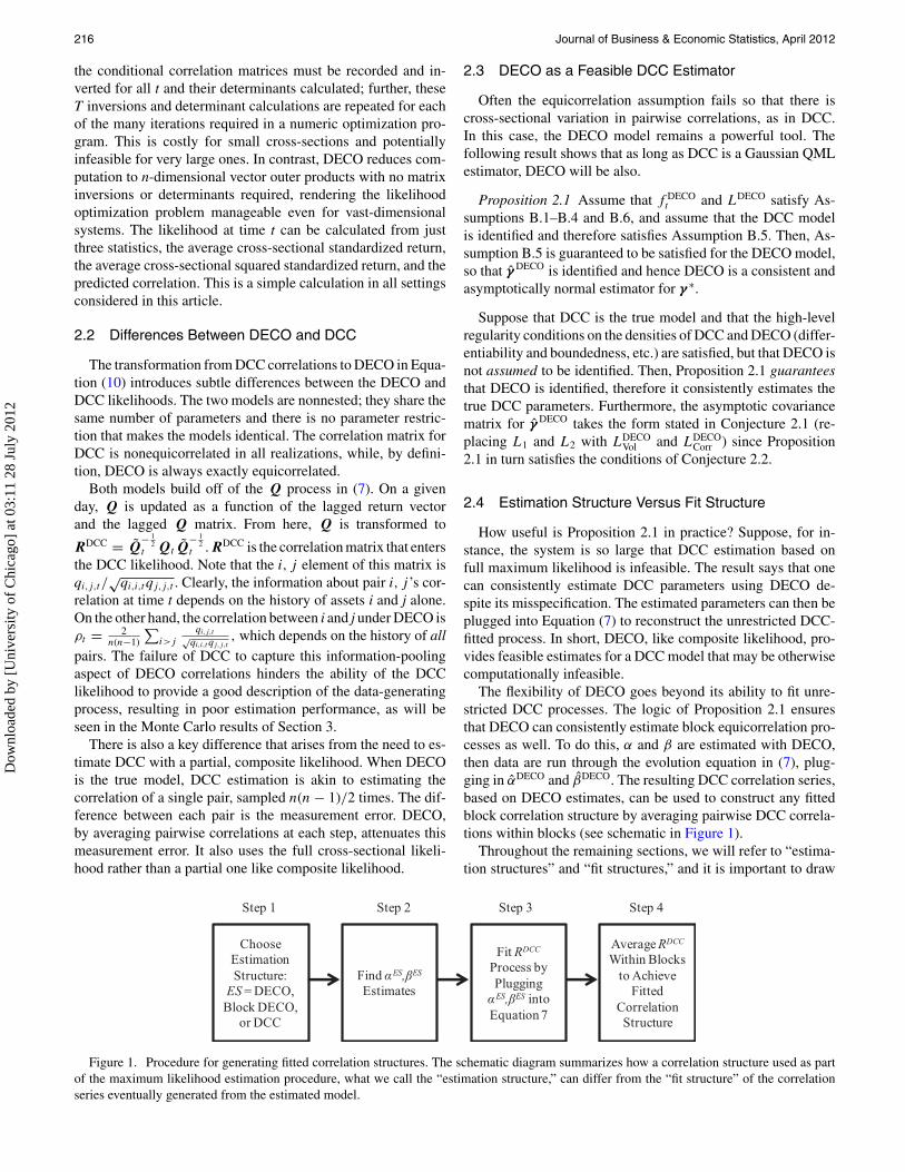
The flexibility of DECO goes beyond its ability to fit unre-stricted DCC processes. The logic of Proposition 2.1 ensuresthat DECO can consistently estimate block equicorrelation pro-cesses as well. To do this, α and β are estimated with DECO,then data are run through the evolution equation in (7), plug-ging in α̂DECO and β̂DECO. The resulting DCC correlation series,based on DECO estimates, can be used to construct any fittedblock correlation structure by averaging pairwise DCC correla-tions within blocks (see schematic in Figure 1).

Throughout the remaining sections, we will refer to “estima-tion structures” and “fit structures,” and it is important to draw

Choose Estimation Structure:

ES = DECO, Block DECO,

or DCC

Find ES, ES

Estimates

Fit RDCC

Process by PluggingES, ES into

Equation 7

Average RDCC

Within Blocks to Achieve

Fitted Correlation Structure

Step 1 Step 2 Step 3 Step 4

Figure 1. Procedure for generating fitted correlation structures. The schematic diagram summarizes how a correlation structure used as partof the maximum likelihood estimation procedure, what we call the “estimation structure,” can differ from the “fit structure” of the correlationseries eventually generated from the estimated model.

Dow

nloa

ded

by [

Uni

vers

ity o

f C

hica

go]

at 0

3:11

28

July

201

2


the distinction between them. The estimation structure is thestructure that the correlation matrix takes within the likelihood.When DECO is used, the estimation structure is a single block.The fit structure, on the other hand, refers to the structure ofthe final, fitted correlation matrices. It is achieved by averagingDCC correlations within blocks after estimation. The resultingblock structure can be different from the estimation structureand might have one block, many blocks, or be unrestricted (asin DCC).

In the next section, we present an alternative estimation ap-proach called Block DECO. Block DECO directly models theblock correlation structure ex ante and makes use of it withinthe estimation procedure. In this case, the estimation structurewill be allowed to have multiple blocks. As with DECO, ex postblock averaging can be used to generate a different desired cor-relation fit structure. With Block DECO as the estimator, fittedcorrelations can have the same, more, or fewer blocks than theestimation structure.

Using DECO with ex post averaging to achieve block cor-relations is, from an implementation standpoint, simpler thanusing full-fledged Block DECO estimation. As will be shown,Block DECO estimation involves composite likelihood and thusis operationally more complex. Ex post averaging achieves thesame outcome of dynamic block correlations with the simplicityof DECO’s Gaussian QML estimation. The advantage of morecomplicated Block DECO estimation is that it can potentiallybe more efficient. We turn to that model now.

2.5 The Block Dynamic Equicorrelation Model

While DECO will be consistent even when equicorrelationis violated, it is possible that a loosening of the structure toblock equicorrelation can improve maximum likelihood esti-mates. In this vein, we extend DECO to take the block structureinto account ex ante and thus incorporate it into the estimationprocedure.

As an example of Block DECO’s usefulness, consider model-ing correlation of stock returns with particular interest in intra-and interindustry correlation dynamics. This may be done byimposing equicorrelation within and between industries. Eachindustry has a single dynamic equicorrelation parameter andeach industry pair has a dynamic cross-equicorrelation parame-ter. With block equicorrelation, richer cross-sectional variationis accommodated while still greatly reducing the effective di-mensionality of the correlation matrix.

This section presents the class of block Dynamic Equicorre-lation models and examines their properties.

Definition 2.3 Rt is a K-block equicorrelation matrix if it ispositive definite and takes the form

Rt =

⎛⎜⎜⎜⎝

(1 − ρ1,1,t )In1 0 · · ·0

. . . 0... 0 (1 − ρK,K,t )InK

⎞⎟⎟⎟⎠

+

⎛⎜⎜⎜⎝

ρ1,1,t Jn1 ρ1,2,t Jn1×n2 · · ·ρ2,1,t Jn2×n1

. . .

... ρK,K,t JnK,

⎞⎟⎟⎟⎠ , (11)

where ρl,m,t = ρm,l,t ∀l, m.

Block DECO specifies that, conditional on the past, each vari-able is Gaussian with mean zero, variance one, and correlationstaking the structure in Equation (11). The return vector r t ispartitioned into K subvectors; each subvector r l contains nl re-turns. The Block DECO correlation matrix, RBD

t , allows distinctprocesses for each of the K diagonal blocks and K(K − 1)/2unique off-diagonal blocks. Blocks on the main diagonal haveequicorrelations following ρl,l,t while blocks off the main diag-onal follow ρl,m,t , where

ρl,l,t = 1

nl(nl − 1)

∑i∈l,j∈l,i �=j


and

ρl,m,t = 1

nlnm

∑i∈l,j∈m


. (12)

The i, j th element of the matrix in (7) is qi,j,t , so Block DECOcorrelations are calculated as the average DCC correlationwithin each block. Despite the block structure of equicorrela-tions, Equation (7) remains the underlying DCC model, thus theparameters α and β do not vary across blocks. Densities, log-likelihoods, and parameter estimates corresponding to BlockDECO model are superscripted with BD in congruence withnotation for the base DECO model.

The following results show the consistency and asymptoticnormality of Block DECO. In analogy to DECO, γ̂ BD is thetwo-stage Gaussian Block DECO estimator assuming returnsare Gaussian and the correlation process obeys Equation (12).

Conjecture 2.4 Assuming that f BDt and LBD satisfy Assump-

tions B.1–B.6 with corresponding unique maximizer γ ∗, thenγ̂ BD is consistent and asymptotically normal for γ ∗.

Further, like DECO, Block DECO is a QML estimator ofDCC models.

Proposition 2.2 Assume that f BDt and LBD satisfy Assump-

tions B.1–B.4 and B.6, and assume that the DCC model is iden-tified and therefore satisfies Assumption B.5. Then, AssumptionB.5 is guaranteed to be satisfied for the Block DECO model,so that γ̂ BD is identified and hence Block DECO is a consistentand asymptotically normal estimator for γ ∗.

The proof follows the same argument as the proof of Propo-sition 2.1. The asymptotic covariance matrix for γ̂ BD takes theform stated in Conjecture 2.1 (replacing L1 and L2 with LBD

Voland LBD

Corr).Block DECO balances the flexibility of unrestricted correla-

tions with the structural simplicity of DECO. However, whenthe number of blocks is greater than two, the analytic forms forthe inverse and determinant of the Block DECO matrix begin tolose their tractability. A special case that remains simple regard-less of the number of blocks occurs when each of the blockson the main diagonal are equicorrelated, but all off-diagonal

Dow

nloa

ded

by [

Uni

vers

ity o

f C

hica

go]

at 0

3:11

28

July

201

2


block equicorrelations are forced to zero. Each diagonal blockconstitutes a small DECO submodel, and therefore its inverseand determinant are known. The full inverse matrix is the blockdiagonal matrix of inverses for the DECO submodels, and itsdeterminant is the product of the submodel determinants.

Conveniently, the composite likelihood method can be usedto estimate Block DECO in more general cases. The compositelikelihood is constructed by treating each pair of blocks as asubmodel, then calculating the quasi-likelihoods of each sub-model, and finally summing quasi-likelihoods over all blockpairs. As discussed by Engle et al. (2008), each pair providesa valid, though only partially informative, quasi-likelihood. Amodel for any number of blocks requires only the analytic in-verse and determinant for a two-block equicorrelation matrixwhen using the method of composite likelihood. The followinglemma establishes the analytic tractability provided by two-block equicorrelation. We suppress t subscripts as all terms arecontemporaneous.

Lemma 2.3 If R is a two-block equicorrelation matrix, thatis, if

R =[

(1 − ρ1,1)In1 0

0 (1 − ρ2,2)In2

]

+[ρ1,1 Jn1×n1 ρ1,2 Jn1×n2

ρ2,1 Jn2×n1 ρ2,2 Jn2×n2

],

then,

i. the inverse is given by

R−1 =[b1 In1 0

0 b2 In2

]+[c1 Jn1×n1 c3 Jn1×n2

c3 Jn2×n1 c2 Jn2×n2

],

where

bi = 1

1 − ρi,i

, i = 1, 2,

c1 = ρ1,1(ρ2,2(n2 − 1) + 1

)− ρ21,2n2

(ρ1,1 − 1)([ρ1,1(n1 − 1) + 1][ρ2,2(n2 − 1) + 1] − n1n2ρ

21,2

) ,c2 = ρ2,2

(ρ1,1(n1 − 1) + 1

)− ρ21,2n1

(ρ2,2 − 1)([ρ1,1(n1 − 1) + 1][ρ2,2(n2 − 1) + 1] − n1n2ρ

21,2

) ,c3 = ρ1,2

n1n2ρ21,2 − (

ρ1,1(n1 − 1) + 1)(

ρ2,2(n2 − 1) + 1) .

ii. the determinant is given by

det(R) = (1 − ρ1,1)n1−1(1 − ρ2,2)n2−1

× [(1 + [n1 − 1]ρ1,1)(1 + [n2 − 1]ρ2,2) − ρ2

1,2n1n2],

iii. R is positive definite if and only if

ρi ∈( −1

ni − 1, 1

), i = 1, 2

and

ρ1,2 ∈(

−√(

ρ1,1(n1 − 1) + 1)(

ρ2,2(n2 − 1) + 1)

n1n2,

√(ρ1,1(n1 − 1) + 1

)(ρ2,2(n2 − 1) + 1

)n1n2

).

With this result in hand, the likelihood function of a two-Block DECO model can, as in the simple equicorrelation case,be written to avoid costly inverse and determinant calculations.

L = −1

2

∑t

(log |Rt | + r ′

t R−1t r t

)

= −1

2

∑t

[log

((1 − ρ1,1,t )

n1−1(1 − ρ2,2,t )n2−1

× [(1 + [n1 − 1]ρ1,1,t )(1 + [n2 − 1]ρ2,2,t ) − ρ2

1,2,t n1n2])

+ r ′t

([b1 In1 0

0 b2 In2

]+[c1 Jn1×n1 c3 Jn1×n2

c3 Jn2×n1 c2 Jn2×n2

])r t

]

= −1

2

∑t

[log

((1 − ρ1,1,t )

n1−1(1 − ρ2,2,t )n2−1

× [(1 + [n1 − 1]ρ1,1,t )(1 + [n2 − 1]ρ2,2,t ) − ρ2

1,2,t n1n2])

+(

b1

n1∑i

r2i,1 + b2

n2∑i

r2i,2 + c1,t

( n1∑i

ri,1

)2

+ 2c3,t

( n1∑i

ri,1

)( n2∑i

ri,2

)+ c2,t

( n2∑i

ri,2

)2)].

In the multiblock case, the above two-block log likelihood iscalculated for each pair of blocks, and then these submodellikelihoods are summed, forming the objective function to bemaximized.

3. CORRELATION MONTE CARLOS

3.1 Equicorrelated Processes

This section presents results from a series of Monte Carlo ex-periments that allow us to evaluate the performance of the DECOframework when the true data-generating process is known. Webegin by exploring the model’s estimation ability when DECOis the generating process. Asset return data for 10, 30, or 100assets are simulated over 1000 or 5000 periods according toEquations (7)–(10). We also consider a range of values for α

and β. For each simulated dataset, we estimate DECO and com-posite likelihood DCC. Here and throughout, we use a subsetof n randomly chosen pairs of assets to form the compositelikelihood in order to speed up computation. In unreported re-sults, we run a subset of our simulations estimating compositelikelihood with all n(n − 1)/2 pairs, and results were virtuallyindistinguishable. Engle et al. (2008) found that the loss fromusing a subset of n pairs is negligible.

Simulations are repeated 2500 times and summary statis-tics for the maximum likelihood parameter estimates are calcu-lated. Table 1 reports the mean, median, and standard deviationof α and β estimates, their average QML asymptotic standard

Dow

nloa

ded

by [

Uni

vers

ity o

f C

hica

go]

at 0

3:11

28

July

201

2


Table 1. Monte Carlo with equicorrelated generating process

DECO Composite likelihood DECO Composite likelihood

α β RMSE α β RMSE α β RMSE α β RMSE

T = 1000 T = 5000α = 0.10, β = 0.80

n = 10 Mean 0.100 0.785 0.015 0.016 0.685 0.053 0.099 0.797 0.007 0.014 0.865 0.051Median 0.099 0.793 0.015 0.824 0.099 0.799 0.014 0.876MeanASE 0.025 0.061 0.007 0.073 0.011 0.025 0.003 0.037Std. Dev. 0.025 0.064 0.009 0.308 0.011 0.024 0.004 0.075



α = 0.05, β = 0.053n = 10 Mean 0.050 0.919 0.015 0.012 0.709 0.053 0.050 0.929 0.007 0.009 0.955 0.049

Median 0.049 0.926 0.011 0.927 0.050 0.929 0.009 0.966MeanASE 0.014 0.026 0.006 0.044 0.006 0.009 0.002 0.008Std. Dev. 0.014 0.050 0.007 0.371 0.006 0.009 0.003 0.092



α = 0.02, β = 0.97n = 10 Mean 0.022 0.928 0.015 0.008 0.548 0.035 0.020 0.969 0.007 0.005 0.824 0.033




Using the DECO model of Equations (7)–(10), return data for 10, 30, or 100 assets are simulated over 1000 or 5000 periods using a range of values for α and β. Then, DECO isestimated with maximum likelihood and DCC is estimated using the (pairwise) composite likelihood of Engle et al. (2008). Simulations are repeated 2500 times and summary statisticsare calculated. The table reports the mean, median, and standard deviation of α and β estimates, as well as their mean quasi-maximum likelihood asymptotic standard error estimates.Asymptotic standard errors are calculated using the “sandwich” covariance estimator of Bollerslev and Wooldridge (1992). We also calculate the root-mean-squared error (RMSE) forthe true versus fitted average pairwise correlation process and report the average RMSE over all simulations. Correlation targeting is used in all cases, thus the intercept is the same forboth models and not reported.

errors (calculated using the “sandwich” covariance estimator ofBollerslev and Wooldridge 1992), and the root-mean-squarederror (RMSE) for the true versus fitted average pairwise corre-lation process. Both models use correlation targeting, thus theintercept matrix is the same for both models and not reported.

The results show that across parameter values, cross-sectionsizes, and sample lengths, DECO outperforms unrestricted DCCin terms of both accuracy and efficiency. Depending on sim-ulation parameters, DECO is between two to 10 times moreaccurate than DCC at matching the simulated average correla-

tion path, as measured by RMSE. In small samples, DCC canfare particularly poorly. For example, when T = 1000, n = 10and β = 0.97, DCC’s mean β estimate is 0.55, versus 0.93 forDECO. Also, DCC’s QML standard errors can grossly under-estimate the true variability of its estimates for all sample sizes.The simulations also show that when the data-generating pro-cess is equicorrelation, increasing the number of assets in thecross section improves estimates.

What explains the poor performance of DCC? Some char-acteristics of the DECO likelihood are lacking in DCC, as

Dow

nloa

ded

by [

Uni

vers

ity o

f C

hica

go]

at 0

3:11

28

July

201

2


discussed in Section 2.2. DCC updates pairwise correlationsusing pairwise data histories, rather than using the data historyof all series as in DECO. Also, the partial information natureof composite likelihood DCC makes it even more difficult forDCC to estimate the parameters of a DECO process.

3.2 Nonequicorrelated Processes

Proposition 2.1 highlights DECO’s ability to consistently es-timate DCC parameters despite violation of equicorrelation. Todemonstrate the performance of DECO in this light, we simu-late series using DCC as the data-generating process (Equations(7) and (8)). Thus, while equicorrelation is violated, the aver-age pairwise correlation behaves according to DECO and theassumptions of Conjecture 2.1 are satisfied. In the correlationevolution, we use an intercept matrix that is nonequicorrelated;the standard deviation of off-diagonal elements is 0.33, demon-strating that the differences in pairwise correlations for the sim-ulated cross sections are substantial.

Again, we generate return data for 10, 30, or 100 assets over1000 or 5000 periods using a range of values for α and β. Next,we estimate both DECO and composite likelihood DCC. Table 2reports summary statistics. DECO exhibits a downward bias inits β estimates that is exacerbated at low values of T/N . Forlarge T/N , the β bias nearly disappears. Composite likelihoodperforms comparatively well, though the difference in accuracyversus DECO is almost indistinguishable when T is 5000. Thesuperior performance of DCC is perhaps most clearly seen in itsexcellent precision. In all cases, the variability of DCC estimatesare a fraction of DECO’s.

It appears that DECO’s performance under misspecifica-tion (Table 2) is overall better than DCC’s performance un-der misspecification (Table 1). Small samples generally resultin a downward bias in DECO estimates, but these estimatesalways manage to stay within one standard error of the es-timates achieved by the correctly specified model. This is incontrast to the severe downward biases displayed by DCC inTable 1. Similarly, DECO’s QML standard errors, while under-stated by an order of magnitude of roughly two, are only mildlybiased compared to the performance of DCC’s standard errors inTable 1.

4. EMPIRICAL ANALYSIS

4.1 Data

Since DECO is motivated primarily as a means of estimatingdynamic covariances for large systems, our sample includesconstituents of the S&P 500 Index. A stock is included if itwas traded over the full horizon 1995–2008 and was a memberof the index at some point during that time. This amounts to466 stocks. Data on returns and SIC codes (which will be usedfor block assignments) come from the CRSP daily file. In ourFactor ARCH regressions and Block DECO estimation, we useFama–French three-factor return data and industry assignments(based on SICs) from Ken French’s website. Precise definitionsof portfolios can be found there.

We also compare average correlations for (Block) DECO andDCC to option implied correlations. For this analysis, we use a

36-stock subset of the S&P sample that were continuously tradedover 1995–2008 and were members of the Dow Jones Industrialsat some point in that period. We also use daily option-impliedvolatilities on these constituents and the index from October1997 through September 2008 from the standardized optionsfile of OptionMetrics.

Before proceeding to the results, we include a brief aside re-garding estimation that will be important for the informationcriterion comparisons we make throughout. All second-stagecorrelation models that we estimate have the same number ofparameters: an α estimate, a β estimate, and n(n − 1)/2 uniqueelements of the intercept matrix. Each factor structure, however,has a different number of parameters. Residual GARCH modelscontain a total of 5n parameters. In addition, the loadings in aK-factor model (including a constant as one of the K factors)contribute an additional nK parameters. Also, the likelihoodsfrom different composite likelihood methods are not directlycomparable because they use submodels of differing dimen-sions. Therefore, we use composite likelihood fitted parametersto evaluate the full joint Gaussian likelihood after the fact, whichis directly comparable to the DECO likelihood.

4.2 Dynamic Equicorrelation in the S&P 500,1995–2008

Our appraisal of DECO has thus far relied on simulated data,now we assess DECO estimates for the S&P 500 sample. As dis-cussed in the section on model estimation, we use a consistenttwo-step procedure to estimate correlations. In the first stage, weregress individual stock returns on a constant and specify resid-uals to be asymmetric GARCH(1,1) processes with Student-tinnovations (Glosten, Jagannathan, and Runkle 1993). GARCHregressions are estimated stock-by-stock via maximum likeli-hood, and then volatility-standardized residuals are given asinputs to the second-stage DECO model. Here and throughout,second-stage models are estimated using correlation targetingfor the intercept matrix Q̄. The first column of Panel A in Ta-ble 3a shows estimates for the basic DECO specification, theirstandard errors, and the Akaike information criterion (AIC) forthe full two-stage log-likelihood.

We find α̂ = 0.021 and β̂ = 0.979, thus the DECO parame-ters are in the range of typical estimates from GARCH models.Rounded to three decimals places, α̂ and β̂ sum to one, indi-cating that the equicorrelation is nearly integrated. Figure 2(a)plots the fitted S&P DECO series against the price level of theS&P 500 Index. The clearest feature of the plot is the tendencyfor the average correlation to rise when the market is decreasingand fall when the market is increasing. This inverse relationshipbetween market value and correlations has been documentedpreviously in the literature. Longin and Solnik (1995, 2001)found that correlations between country level indices are higherduring bear markets and in volatile periods. Ang and Chen(2002) found the same result for correlations between portfo-lios of U.S. stocks and the aggregate market. Our results showthat, over the past 15 years, correlations reached their highestlevel during the global crisis in the last four months of 2008,when the average correlation between S&P 500 stocks reachednearly 60%.

Dow

nloa

ded

by [

Uni

vers

ity o

f C

hica

go]

at 0

3:11

28

July

201

2


Table 2. Monte Carlo with nonequicorrelated generating process

DECO Composite likelihood DECO Composite likelihood

α β RMSE α β RMSE α β RMSE α β RMSE

T = 1000 T = 5000α = 0.10, β = 0.80




α = 0.05, β = 0.009n = 10 Mean 0.052 0.905 0.015 0.051 0.922 0.009 0.050 0.928 0.007 0.050 0.929 0.004




α = 0.02, β = 0.097n = 10 Mean 0.026 0.888 0.014 0.023 0.954 0.011 0.020 0.967 0.007 0.021 0.968 0.004




Using the DCC model of Equations (7) and (8), return data for 10, 30, or 100 assets are simulated over 1000 or 5000 periods using a range of values for α and β. Then, DECO isestimated with maximum likelihood and DCC is estimated using the (pairwise) composite likelihood of Engle et al. (2008). Simulations are repeated 2500 times and summary statisticsare calculated. The table reports the mean, median, and standard deviation of α and β estimates, as well as their mean quasi-maximum likelihood asymptotic standard error estimates.Asymptotic standard errors are calculated using the “sandwich” covariance estimator of Bollerslev and Wooldridge (1992). We also calculate the root-mean-squared error (RMSE) forthe true versus fitted average pairwise correlation process and report the average RMSE over all simulations. Correlation targeting is used in all cases, thus the intercept is the same forboth models and not reported.

4.3 Factor ARCH DECO

As discussed in the Introduction, DECO may be used to modelresiduals from a factor model of returns. As a simple exam-ple, consider a one factor model for returns: rj = βj rm + ej .If the factor rm (and each idiosyncrasy ej ) obeys a univariateGARCH model and if the vector of idiosyncrasies e is dy-namically equicorrelated, then we call this a Factor (Double)ARCH DECO model. (See Engle 2009b for additional detail onappending multivariate GARCH models to factor model residu-als.) The log-likelihood of a factor model decomposes additively

since log fr,t (r t ) = log fr,t (r t |Factorst) + log fFactors,t(Factorst).An additive log-likelihood can be maximized by maximizingeach element of the sum separately, thus the volatility and corre-lations of factors can be estimated separately from the volatilityand correlations of residuals and estimates will be consistent.

Our next empirical result demonstrates the usefulness ofDECO in capturing lingering dynamics among correlations offactor model residuals. We consider two factor structures forreturns: the CAPM and the Fama–French (1993) three-factormodel. In both cases, the first-stage models are regressions

Dow

nloa

ded

by [

Uni

vers

ity o

f C

hica

go]

at 0

3:11

28

July

201

2


1995 1997 1999 2001 2003 2005 2007 20090

500

1000

1500

S&P

500

Lev

el

1995 1997 1999 2001 2003 2005 2007 2009

20%

40%

60%

DE

CO

1995 1997 1999 2001 2003 2005 2007 20090

500

1000

1500

S&P

500

Lev

el

1995 1997 1999 2001 2003 2005 2007 2009

2%

4%

6%

DE

CO

1995 1997 1999 2001 2003 2005 2007 20090

500

1000

1500

S&P

500

Lev

el

1995 1997 1999 2001 2003 2005 2007 2009

2%

3%D

EC

O

(b)

(c)

(a)

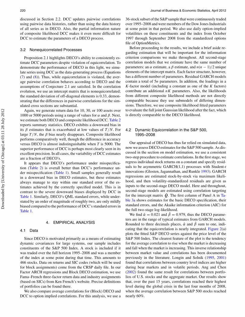
Figure 2. Fitted dynamic equicorrelation by factor model, S&P 500 constituents, 1995–2008. The figure shows fitted residual equicorrelationsof S&P 500 constituents estimated with the DECO model (black line) and the S&P 500 index level (gray area). Equicorrelation fits are basedon model estimates in the first column of Table 3. The graphs correspond to the following factor schemes: (a) no factor, (b) the Sharpe–LintnerCAPM, and (c) the Fama–French (1993) three-factor model.

Dow

nloa

ded

by [

Uni

vers

ity o

f C

hica

go]

at 0

3:11

28

July

201

2


Table 3a. Full-sample correlation estimates for S&P 500 constituents,1995–2008

DECO 10-Block DCC

Panel A: No Factorα 0.021 0.023 0.014

0.003 0.007 0.005β 0.979 0.975 0.975

0.003 0.008 0.034AIC –6802.0 –6861.6 –6735.0

Panel B: CAPM Market Factorα 0.006 0.008 0.005

0.005 0.010 0.004β 0.986 0.982 0.986

0.016 0.028 0.019AIC –6851.4 –6921.9 –7182.2

Panel C: Fama–French 3 Factorsα 0.010 0.002 0.004

0.005 0.001 0.003β 0.804 0.998 0.984

0.114 0.001 0.029AIC –6899.2 –6955.2 –7270.2

The table presents estimation results for nine dynamic covariance models. Each model is atwo-stage quasi-maximum likelihood estimator and is a combination of one of three first-stage models with one of three second-stage models. The first-stage models are GARCHregression models imposing a factor structure for the cross section of returns, in whichthe structures are no factor (Panel A), the Sharpe–Lintner one-factor CAPM (Panel B),and the Fama–French (1993) three-factor model (Panel C). The second-stage correlationmodels, estimated on standardized residuals from the first stage, are one- and 10-BlockDECO and composite likelihood DCC. Below each estimate, we report quasi-maximumlikelihood asymptotic standard errors in italics. Asymptotic standard errors are calculatedusing the “sandwich” covariance estimator of Bollerslev and Wooldridge (1992). For eachmodel, we report the Akaike information criterion calculated using the sum of the first- andsecond-stage log likelihoods penalized for the number of parameters in both stages. Theanalysis is performed on the S&P 500 dataset described in Section 4.

of individual stock returns on a set of factors where, as be-fore, all factors and idiosyncrasies are modeled as asymmet-ric GARCH(1,1). The second-stage is estimated with the basicDECO specification. Estimation results are shown in the firstcolumn of Panels B and C in Table 3(a). CAPM residual cor-relations are slightly less persistent than the no factor case,with α̂ + β̂ = 0.992. Adding the market factor substantially in-creases the log-likelihood, even after accounting for its addi-tional parameters (as seen by the decreased AIC versus column1 of Panel A). CAPM residual correlations are plotted againstS&P 500 Index price level in Figure 2(b). On average, the resid-ual correlation is very low, dropping to less than 2% for mostof the sample from a time average of over 20% with no factor(Figure 2(a)). The most striking feature of this plot is the largeincrease in residual correlations from 1999 through late 2001,corresponding to the rise and fall of the technology bubble. Itappears that, before and after the tech boom, the CAPM does avery good job of describing return correlations. During the techepisode, an additional factor seems to surface. The impact ofthis factor on dependence among assets is not captured by theCAPM, but is picked up by residual DECO.

Estimates for residual correlations using the Fama–Frenchthree-factor model show much weaker dynamics among residualcorrelations, as persistence drops to α̂ + β̂ = 0.814. Includingthree factors further improves the AIC. Figure 2(c) shows thatresidual correlations are almost always about 1.5% and flat. The

only exceptions are brief spikes to 3% during the peak of thetech bubble and the crisis of late 2008.

4.4 Comparing DECO and DCC Correlations

The previous subsections have explored DECO fits using nofactor structure, the one-factor CAPM, and the Fama–Frenchthree-factor model. We now examine the fits of DCC for each ofthese three first-stage models to compare with DECO. DCC isestimated using composite likelihood with submodels that arepairs of stocks; n of the possible n(n − 1)/2 pairs are randomlyselected as submodels, where n = 466 for our sample. The useof a large subset of all pairs reduces computation time whilenegligibly degrading the performance of the estimator (as sug-gested by Engle et al. 2008). As a check of this point, we useall pairs for estimating composite likelihood DCC in a smallercross-section of 36 Dow Jones constituents (a subset of our S&Psample) and find that the results are nearly identical to the resultswhen only 36 randomly selected pairs are used.

DCC parameter estimates are shown in the third column ofTable 3(a). When no factor is used, parameter estimates forDECO and DCC are similar and within two standard errors ofeach other. DECO achieves a lower AIC, making it the bettermodel according to this criterion. Note, DECO and DCC use thesame number of parameters, so the lower AIC for DECO is duesolely to its better likelihood fit. We next evaluate how muchpairwise DCC correlations deviate from the equicorrelation se-ries of DECO. Figure 3(a) plots DECO against the 25th, 50th,and 75th percentile of pairwise DCC correlations when the firststage model has no factor. These quartiles give a sense of the dis-persion of pairwise correlations. As the figure shows, the upperand lower quartiles are almost always within 5% of the me-dian, and the dynamic pattern of the quartiles closely track theequicorrelation. The similar correlation dynamics for pairs ofstocks and for equicorrelation is consistent with DECO’s abilityto achieve a superior fit.

When the first-stage model includes the CAPM market fac-tor, DCC α and β estimates again are very close to those ofDECO. In this case, DCC fits the data better according to theAkaike criterion. To understand how DCC might provide a bet-ter fit, consider the DCC residual correlation quartiles shown inFigure 3(b). We see first that the dispersion of correlations hasincreased relative to the average correlation. Residual equicor-relation is roughly 2–3% over time, while the 75th and 25thDCC percentiles are around 6% and –3% on average. Further-more, other than during the technology bubble, there appearsto be no systematic relationship between the time series patternin equicorrelation and the pattern of pairwise correlations. Thispicture therefore suggests that the ability of DECO to describeresidual CAPM correlations is limited, consistent with the AICvalues we find.

Using the Fama–French model reinforces the notion that DCCis a more apt descriptor of factor model residuals due to the ten-dency for residual pairwise correlations to exhibit idiosyncraticdynamics. Table 3(a), Panel C shows that DCC continues tofind stronger dynamics in correlations than DECO in terms of α

and β estimates, and pairwise DCC correlations in Figure 3(c)are quite distinct from the equicorrelation in their time series

Dow

nloa

ded

by [

Uni

vers

ity o

f C

hica

go]

at 0

3:11

28

July

201

2


(a)

(b)

(c)

1995 1997 1999 2001 2003 2005 2007 20090

0.1

0.2

0.3

0.4

0.5

0.6C

orre

latio

nOne-Block DECOPairwise 75th PercentilePairwise MedianPairwise 25th Percentile

1995 1997 1999 2001 2003 2005 2007 2009

-0.04

-0.02

0

0.02

0.04

0.06

0.08

0.1

0.12

Cor

rela

tion

One-Block DECOPairwise 75th PercentilePairwise MedianPairwise 25th Percentile

1995 1997 1999 2001 2003 2005 2007 2009

-0.03

-0.02

-0.01

0

0.01

0.02

0.03

0.04

0.05

0.06

0.07

Cor

rela

tion

One-Block DECOPairwise 75th PercentilePairwise MedianPairwise 25th Percentile

Figure 3. The figure shows fitted correlations of S&P 500 Con-stituents, 1995–2008. The figure shows fitted correlations of S&P 500constituents estimated with DECO and DCC. Correlation fits are basedon model estimates in Table 3. The graphs correspond to the follow-ing first-stage factor schemes: (a) no factor, (b) the Sharpe–LintnerCAPM, and (c) the Fama–French (1993) three-factor model. Each plotshows the fitted one-block equicorrelation and the 25th, 50th, and 75thpercentile of pairwise DCC correlations in each period.

behavior. In summary, our results elucidate the conditions underwhich DECO can provide a good description of the data. Whencomovement among all pairs shows broadly similar time seriesdynamics, DECO fits well and outperforms DCC. Conversely,when dynamics in pairwise correlations are dissimilar, DCCmay be a more appropriate model.

4.5 Block DECO

In our last description of correlations among S&P con-stituents, we repeat the above analyses using 10-Block DECOas the correlation estimator. Stocks are assigned to blocksbased on SIC codes according to the industry classificationscheme for Ken French’s 10 industry portfolios. We esti-mate 10-Block DECO using Gaussian composite likelihoodwith submodels that are pairs of blocks. Due to the lownumber of blocks, all 10(10 − 1)/2 pairs of industries areused to form the Block DECO composite likelihood. In par-ticular, when formulating the likelihood contribution of in-dustry pair i, j , a total of ni + nj stocks are used in thesubmodel.

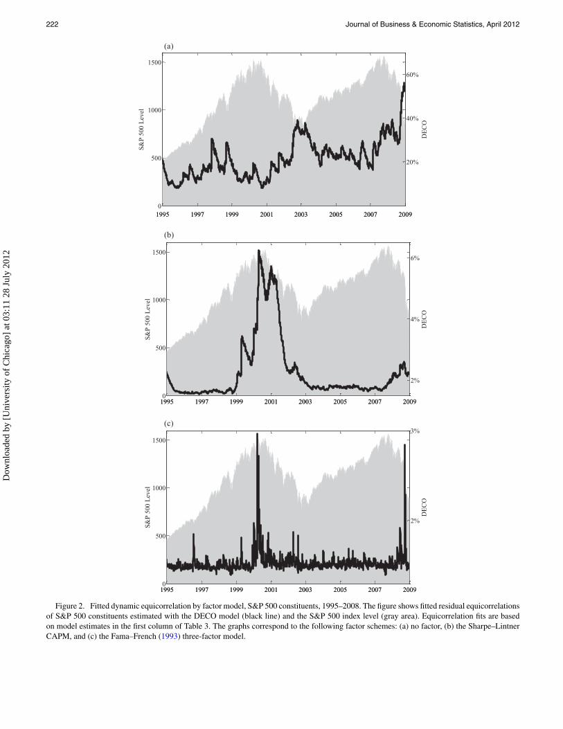
When no factors are used in the first-stage GARCH regres-sions, Block DECO achieves a better AIC than both DCC andDECO, and finds similar parameter estimates. To get a senseof the flexibility Block DECO adds to the correlation structure,Figure 4 plots within-industry correlations for energy, telecom,and health stocks. We choose only three of the 10 sectors to keepthe plot legible while illustrating the richness a block structurecan add to the cross-section of correlations. A few interestingpatterns emerge. First, the correlation among energy stocks hasslowly trended upward over the entire sample. While correla-tions were low for the market as a whole over 2004–2007, energycorrelations remained high and continued to climb. Telecomstocks, meanwhile, had the sharpest rise in correlations in themarket downturn following the technology boom. Health stocksmaintained relatively low correlations throughout the sample.All three groups, however, experience drastic increases in cor-relations during late 2008, at which time all groups saw theirhighest level of comovement.

We also estimate Block DECO on residuals from the CAPMand Fama–French model. While Block DECO achieves a bet-ter fit than DECO in these factor models, DCC maintains thesuperior AIC. Block DECO, like DCC, finds more persistent dy-namics in correlations for Fama–French residuals than DECO.

4.6 Equicorrelation and Implied Correlations, DowJones Index

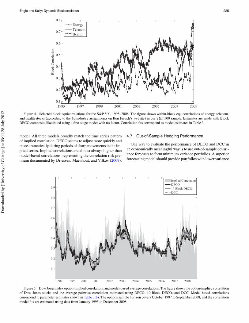
Options traded on an index and its members provide an oppor-tunity to validate fits from correlation models against forward-looking implied correlations that are based solely on optionsprices. We briefly compare fitted correlations from DECO andDCC to option-implied correlations. Since options do not ex-ist for all members of the S&P 500, we instead examine theDow Jones Index, for which liquid options are traded on allconstituents. Our sample of options data for the Dow Jones andits members begins in October 1997 (when Dow Jones Indexoptions were introduced) through September 2008. Implied cor-relation is calculated from implied volatilities of the index andits constituents as in Equation (1). We use implied volatilities oncall options standardized to have one month to maturity, avail-able from OptionMetrics. We also estimate DECO, 10-BlockDECO, and DCC using daily returns on Dow Jones stocks from1995–2008. The first-stage model in all cases has no factors.Estimates are reported in Table 3(b). Figure 5 plots the impliedcorrelation against the average fitted pairwise correlation of each

Dow

nloa

ded

by [

Uni

vers

ity o

f C

hica

go]

at 0

3:11

28

July

201

2


1995 1997 1999 2001 2003 2005 2007 20090.1

0.2

0.3

0.4

0.5

0.6

0.7

0.8

Blo

ck C

orre

lati

on

EnergyTelecomHealth

Figure 4. Selected block equicorrelations for the S&P 500, 1995–2008. The figure shows within-block equicorrelations of energy, telecom,and health stocks (according to the 10 industry assignments on Ken French’s website) in our S&P 500 sample. Estimates are made with BlockDECO composite likelihood using a first-stage model with no factor. Correlation fits correspond to model estimates in Table 3.

model. All three models broadly match the time series patternof implied correlation. DECO seems to adjust more quickly andmore dramatically during periods of sharp movements in the im-plied series. Implied correlations are almost always higher thanmodel-based correlations, representing the correlation risk pre-mium documented by Driessen, Maenhout, and Vilkov (2009).

4.7 Out-of-Sample Hedging Performance

One way to evaluate the performance of DECO and DCC inan economically meaningful way is to use out-of-sample covari-ance forecasts to form minimum variance portfolios. A superiorforecasting model should provide portfolios with lower variance

1998 1999 2000 2001 2002 2003 2004 2005 2006 2007 2008

0.1

0.2

0.3

0.4

0.5

0.6

0.7

0.8

0.9

Implied CorrelationDECO10-Block DECODCC

Figure 5. Dow Jones index option-implied correlations and model-based average correlations. The figure shows the option-implied correlationof Dow Jones stocks and the average pairwise correlation estimated using DECO, 10-Block DECO, and DCC. Model-based correlationscorrespond to parameter estimates shown in Table 3(b). The options sample horizon covers October 1997 to September 2008, and the correlationmodel fits are estimated using data from January 1995 to December 2008.

Dow

nloa

ded

by [

Uni

vers

ity o

f C

hica

go]

at 0

3:11

28

July

201

2


Table 3b. Full-sample correlation estimates for Dow Jonesconstituents, 1995–2008

DECO 10-Block DCC

α 0.034 0.023 0.0190.005 0.010 0.005

β 0.964 0.971 0.9700.005 0.013 0.007

AIC –572.7 –581.3 –577.4

This table repeats the analysis of Table 3(a), Panel A (no factor) for the subsample of 36Dow Jones constituents.

than portfolios formed based on competing models. This typeof comparison is motivated by the well-known mean–varianceoptimization setting of Markowitz (1952). Consider a collectionof n stocks with expected return vector µ and covariance matrix�. Two hedge portfolios of interest are the global minimumvariance (GMV) portfolio and the minimum variance portfoliosubject to achieving an expected return of at least q. The GMVportfolio weights are the solution to the problem

minω

ω′�ω s.t. ω′ι = 1.

The MV portfolio is found by solving this problem subject tothe additional constraint ω′µ ≥ q. The expressions for optimalweights are

ωGMV = 1

A�−1ι and

ωMV = C − qB

AC − B2�−1ι + qA − B

AC − B2�−1µ, (13)

where A = ι′�−1ι, B = ι′�−1µ and C = µ′�−1µ.We focus on two forecasting questions. The first is motivated

by Elton and Gruber (1973), who demonstrated that minimumvariance portfolio choices can be improved by averaging pair-wise correlations within groups. Our question extends this ideato the conditional setting, and is linked to the question of bestcorrelation fit structure to employ with ex post averaging. OnceDECO is estimated, it can be used to form out-of-sample unre-stricted pairwise correlation forecasts (as in DCC). These pair-wise correlations can then be used to form different fitted cor-relation structures by averaging pairwise correlation forecastswithin blocks as discussed in Section 2.4 and outlined in Fig-ure 1. Ultimately, DECO estimates can be used to construct cor-relation forecasts that are equicorrelated, block equicorrelated,or unrestricted. By varying the choice of correlation structurein our forecasts, we can evaluate the portfolio choice benefit ofaveraging pairwise correlations in a conditional setting (whilekeeping the estimation structure fixed as basic DECO).

Our experiment proceeds as follows. Using daily returns ofthe S&P cross-section for the five-year estimation window be-ginning in January 1995 and ending December 1999, we

1. Estimate first-stage factor volatility models for each stock2. Use estimates of regression/volatility models to form one-

step ahead volatility forecasts for each stock3. Using devolatized residuals from the first stage, estimate the

second-stage correlation model

4. Use correlation model parameter estimates to forecast unre-stricted pairwise correlations one step ahead

5. Conduct ex post averaging of pairwise correlations to achieveeach of the following correlation forecast fit structures (i) un-restricted, (ii) 30 industry blocks, (iii) 10 industry blocks, and(iv) a single block

6. Combine correlation forecasts for each fit structure with re-gression/volatility model estimates and forecasts to constructthe full covariance matrix forecast

7. Plug the resulting covariance forecast into (13) to find opti-mal portfolio weights (this step also requires an estimate ofmean return µ. We set µ equal to the historical mean andchoose q = 10% annually)

8. Record realized returns for portfolios based on forecasts.

One-step-ahead forecasts and portfolio choices are made inthis manner for the next 22 days. After 22 days, the second-stage model is reestimated and the new parameters are usedto generate the one-day ahead forecasts for the next 22 daysand new out-of-sample portfolio returns are calculated. This isrepeated until all data through December 2008 have been used.The result is a set of 2263 out-of-sample GMV and MV portfolioreturns for each model.

After completing the forecasting procedure and recordingportfolio returns, we calculate the realized daily variance foreach ex post correlation fit structure. A superior model will pro-duce optimal portfolios with lower variance realizations. Wecan test the significance of differences between portfolio vari-ances for different correlation fit structures with a Diebold andMariano (2002) test between the vectors of squared returns foreach method. These tests are also related to the tests of Engleand Colacito (2006).

Out-of-sample GMV portfolio standard deviations when thefirst-stage has no factors model are reported in the first columnof Table 4. A 30-block fit structure generates the lowest varianceGMV portfolio with a standard deviation of 0.0093. This im-proves over the next best ex post structure, which used 10 blocksand achieves a standard deviation of 0.0096. The difference issignificant at the 0.1% one-sided significance level. The sameresult is found for MV portfolios.

We repeat the hedging experiment using the CAPM andFama–French factor structures. When the CAPM is used, ex postaveraging over 10 blocks takes over the lowest variance posi-tion, significantly outperforming the second best (unrestricted)structure at the 2.5% one-sided significance level. The 10-blockfit structure also achieves the lowest variance MV portfolio,though its improvement is not statistically significant over thenext best model. For the Fama–French model, the unrestrictedfit becomes the superior structure and significantly outperforms(block) equicorrelated structures.

DECO’s minimum variance portfolio results so far suggestthat there can be hedging benefits to varying the block struc-ture of correlations after estimation. These results, however, donot speak about the estimation ability of different correlationmodels. If the same exercises were repeated using different cor-relation models than DECO to estimate α and β, how wouldportfolio choices fare?

Table 5 reports the standard deviations of GMV and MV port-folios when 10-Block DECO and DCC are used for estimation.

Dow

nloa

ded

by [

Uni

vers

ity o

f C

hica

go]

at 0

3:11

28

July

201

2


Table 4. DECO Out-of-sample minimum variance portfolio comparison (by ex post fit structure)

GMV MV

Estimation structure Fit structure No factor CAPM FF3 No factor CAPM FF3

DECO Unrestricted 0.0117 0.0090 0.0073 0.0106 0.0086 0.0073∗∗∗ ∗∗∗

30-Block 0.0093 0.0093 0.0091 0.0088 0.0090 0.0091∗∗∗ ∗∗∗

10-Block 0.0096 0.0090 0.0087 0.0090 0.0086 0.0086∗∗ ∗

1-Block 0.0101 0.0100 0.0091 0.0096 0.0098 0.0091

The table presents the results of an out-of-sample portfolio formation experiment to test covariance forecasting ability. The following procedure is used to create sequential, nonoverlappingcovariance forecasts, which are then used to form portfolios. First, the covariance model is estimated using a cross-section of daily returns for the five-year estimation window beginningJanuary 1995 and ending December 1999, and one-step-ahead covariance forecasts for the next 22 days are formed. Using each day’s forecast, we construct the global minimum variance(GMV) portfolio and the minimum variance (MV) portfolio subject to a 10% required annual return (see Section 4) and record the return for each portfolio that day. Data from the22-day forecast period is then added to the estimation sample and the model is reestimated. The new estimates are used to generate covariance forecasts for the subsequent 22 daysand new out-of-sample portfolio returns are calculated. This is repeated until all data through December 2008 has been used. The result is a set of 2263 out-of-sample GMV and MVportfolio returns. The table reports standard deviations of the portfolio return time series. Three different first-stage models, which are factor structures for the cross-section of returns,are considered (1) no factor (2) the Sharpe–Lintner CAPM, and (3) the Fama–French (1993) three-factor model. The second-stage model is DECO, estimated on standardized residualsfrom the first stage. Portfolios are formed with four different ex post correlation fit structures based on industry assignment, as described in Section 4. Within each column, the correlationforecasting method that achieves the lowest standard deviation portfolio is shown in bold. A Diebold–Mariano test is calculated for the significance of the best model against the secondbest model in the same column. The best model is accompanied by *, **, or *** if it achieves a lower standard deviation than the next best model at the 2.5%, 1.0%, or 0.1% (one-sided)level, respectively. The analysis is performed on the S&P 500 dataset described in Section 4.

For ease of reference and to conduct a new set of hypothesistests, we reproduce DECO’s results from Table 4. The table hasa column for each first-stage factor model. Within a column,we report portfolio standard deviations achieved across differ-ent estimation and fit structures for correlations. Then, withincolumns (i.e., for a given factor structure), Diebold–Marianotests are performed to compare the variances achieved by DECOand Block DECO against the base case of DCC, holding the cor-

relation fit structure fixed. For instance, the variance of DECOwith an unrestricted fit structure is tested against DCC with anunrestricted structure, and 10-Block DECO with a 30-block fitis compared against DCC with a 30-block fit. In this way, wecan test whether (Block) DECO chooses significantly superiorportfolios, holding the correlation fit structures fixed.

When the first-stage model includes no factors, the bestoverall GMV portfolio performance is achieved by estimating

Table 5. Out-of-sample minimum variance portfolio comparison (by correlation and factor model)

GMV MV

Estimation structure Fit structure No factor CAPM FF3 No factor CAPM FF3

DECO Unrestricted 0.0117 0.0090 0.0073 0.0106 0.0086 0.007330-Block 0.0093 0.0093 0.0091 0.0088 0.0090 0.0091

∗∗∗ ∗∗ ∗∗ ∗ ∗∗ ∗∗∗

10-Block 0.0096 0.0090 0.0087 0.0090 0.0086 0.0086∗∗ ∗∗ ∗∗∗ ∗∗

1-Block 0.0101 0.0100 0.0091 0.0096 0.0098 0.009110-Block DECO Unrestricted 0.0112 0.0097 0.0077 0.0102 0.0091 0.0077

∗

30-Block 0.0094 0.0093 0.0091 0.0088 0.0090 0.0092∗ ∗

10-Block 0.0096 0.0091 0.0087 0.0090 0.0087 0.00881-Block 0.0101 0.0101 0.0091 0.0096 0.0099 0.0091

DCC Unrestricted 0.0118 0.0091 0.0073 0.0105 0.0086 0.007330-Block 0.0094 0.0093 0.0091 0.0088 0.0090 0.009110-Block 0.0096 0.0091 0.0087 0.0089 0.0087 0.00871-Block 0.0101 0.0100 0.0092 0.0096 0.0098 0.0091

The table presents the results of an out-of-sample portfolio formation experiment to test covariance forecasting ability. The following procedure is used to create sequential, nonoverlappingcovariance forecasts, which are then used to form portfolios. First, a covariance model is estimated using a cross-section of daily returns for the five-year estimation window beginningJanuary 1995 and ending December 1999, and one-step-ahead covariance forecasts for the next 22 days are formed. Using each day’s forecast, we construct the global minimum variance(GMV) portfolio and the minimum variance (MV) portfolio subject to a 10% required annual return (see Section 4) and record the return for each portfolio that day. Data from the22-day forecast period is then added to the estimation sample and the model is reestimated. The new estimates are used to generate covariance forecasts for the subsequent 22 daysand new out-of-sample portfolio returns are calculated. This is repeated until all data through December 2008 has been used. The result is a set of 2263 out-of-sample GMV and MVportfolio returns. The table reports standard deviations of the portfolio return time series. Three different first-stage models, which are factor structures for the cross section of returns,are considered (1) no factor (2) the Sharpe–Lintner CAPM, and (3) the Fama–French (1993) three-factor model. Three second-stage models, DECO, 10-Block DECO, and DCC, areestimated on standardized residuals from the first stage. Portfolios are formed with four different ex post correlation fit structures based on industry assignment, as described in Section 4.Within each column, the correlation forecasting method that achieves the lowest standard deviation portfolio is shown in bold. A Diebold–Mariano test is calculated for the significanceof difference between each structure/fit pair (for DECO and Block DECO) against the same fit structure based on DCC estimates. Values accompanied by *, **, or *** achieve a lowerstandard deviation than their DCC counterpart at the 2.5%, 1.0%, or 0.1% (one-sided) level, respectively. The analysis is performed on the S&P 500 dataset described in Section 4.

Dow

nloa

ded

by [

Uni

vers

ity o

f C

hica

go]

at 0

3:11

28

July

201

2


DECO, then using parameter estimates to construct 30-blockcorrelation matrices ex post. This superior performance is sta-tistically significant compared to DCC with 30-block fit struc-ture. Block DECO also manages to significantly outperformDCC when the ex post structure has 30 blocks or is unrestricted.When a market factor or Fama–French factors are included,DECO continues to be the best estimation model, though itsoutperformance loses significance in the Fama–French case.The results are essentially the same for MV portfolios, with theexception that block-DECO becomes the best estimator for thefirst-stage model without a factor.

What qualitative assessments can we make from this analy-sis? First, the results highlight that tailoring the ex post blockstructure, regardless of the correlation estimator, can providesubstantial improvement in hedging performance, corroborat-ing evidence from a long strand of literature on unconditionalportfolio choice. Second, it appears that (Block) DECO, besidesoffering a relatively good in-sample fit of the data as shown inTable 3a, provides statistically superior out-of-sample correla-tion forecasts compared with DCC. We interpret this as evidencethat DECO can be a valuable way of dealing with noisy pairwisecorrelations during estimation.

5. CONCLUSION

DECO represents a major simplification in modeling timevarying conditional covariance matrices for returns of an arbi-trary number of assets. The equicorrelation assumption can beused to reduce noise and improve portfolio selection procedures,and it is a simplifying assumption that arises naturally in a vari-ety of financial contexts. We extend the model to accommodateequicorrelated blocks which can be used to ease the restrictive-ness of DECO while maintaining its simplicity and robustness.DECO and Block DECO are valuable models in the presence ofnonequicorrelated variables. We prove quasi-maximum likeli-hood results that ensure (Block) DECO is a consistent estimatoreven when the true correlation process follows DCC. The theo-retical properties of DECO are confirmed in experiments usingsimulated systems. For constituents of the S&P 500 Index, es-timates show that DECO provides a superior fit in the senseof information criteria relative to DCC. A test of forecastingperformance shows that DECO can be used to construct out-of-sample hedge portfolios with significantly lower variance thanthose based on DCC.

ACKNOWLEDGMENT

The authors thank two anonymous referees, the associate ed-itor, and editors Arthur Lewbel and Jonathan Wright for help-ful comments. Kelly’s research was supported in part by theNeubauer Family Foundation.

[Received February 2008. Revised July 2011.]

REFERENCES

Aielli, G. (2009), “Dynamic Conditional Correlations: On Properties and Esti-mation,” Working Paper, University of Florence. [215]

Ang, A., and Chen, J. (2002), “Asymmetric Correlations of Equity Portfolios,”Journal of Financial Economics, 63(3), 443–494. [220]

Bauwens, L., Laurent, S., and Rombouts, J. (2006), “Multivariate GARCHModels: A Survey,” Journal of Applied Econometrics, 21(1), 79–109. [212]

Berndt, E., and Savin, N. (1975), “Estimation and Hypothesis Testing in SingularEquation Systems with Autoregressive Disturbances,” Econometrica, 43(5),937–957. [213]

Bollerslev, T., Engle, R., and Nelson, D. (1994), “ARCH Models,” Handbookof Econometrics, 4, 2959–3038. [212]

Bollerslev, T., and Wooldridge, J. (1992), “Quasi-Maximum Likelihood Esti-mation and Inference in Dynamic Models With Time-Varying Covariances,”Econometric Reviews, 11(2), 143–172. [219,221]

Diebold, F., and Mariano, R. (2002), “Comparing Predictive Accuracy,” Journalof Business and Economic Statistics, 20(1), 134–144. [226]

Driessen, J., Maenhout, P., and Vilkov, G. (2009), “Option-Implied Corre-lations and the Price of Correlation Risk,” Journal of Finance, 1377–1406. [225]

Elton, E., and Gruber, M. (1973), “Estimating the Dependence Structure ofShare Prices—Implications for Portfolio Selection,” Journal of Finance,28(5), 1203–1232. [213,226]

Engle, R. (2002), “Dynamic Conditional Correlation: A Simple Class ofMultivariate Generalized Autoregressive Conditional HeteroskedasticityModels,” Journal of Business and Economic Statistics, 20(3), 339–350. [212,215]

——— (2009a), Anticipating Correlations, A New Paradigm for Risk Manage-ment, Princeton, NJ: Princeton University Press. [212]

——— (2009b), “High Dimension Dynamic Correlations,” in The Methodologyand Practice of Econometrics: A Festschrift in Honour of David F. Hendry,pp. 122–148. [212,221]

Engle, R., and Colacito, R. (2006), “Testing and Valuing Dynamic Correlationsfor Asset Allocation,” Journal of Business and Economic Statistics, 24(2),238–253. [226]

Engle, R., Ng, V., and Rothschild, M. (1990), “Asset Pricing With a Factor-ARCH Covariance Structure: Empirical Estimates for Treasury Bills,” Jour-nal of Econometrics, 45, 213–237. [212]

Engle, R., Ng, V., and Rothschild, M. (1992), “A Multi-Dynamic-FactorModel for Stock Returns,” Journal of Econometrics, 52(1–2), 245–266. [212]

Engle, R., and Rangel, J. (2012), “The Factor-Spline-GARCH Model for Highand Low Frequency Correlations,” Journal of Business and Economic Statis-tics, 30(1), 109–124. [212]

Engle, R., Shephard, N., and Sheppard, K. (2008), “Fitting Vast DimensionalTime-Varying Covariance Models,” Working Paper, Oxford University.[212,218,221,223]

Engle, R., and Sheppard, K. (2005), “Theoretical and Empirical Properties ofDynamic Conditional Correlation Multivariate GARCH,” Working Paper,Oxford University. [212,215]

Fama, E., and French, K. (1993), “Common Risk Factors in the Returns onStocks and Bonds,” Journal of Financial Economics, 33(1), 3–56. [223,227]

Glosten, L., Jagannathan, R., and Runkle, D. (1993), “On the Relation Betweenthe Expected Value and the Volatility of the Nominal Excess Return onStocks,” Journal of Finance, 48(5), 1779–1801. [220]

Jagannathan, R., and Ma, T. (2003), “Risk Reduction in Large Portfolios: WhyImposing the Wrong Constraints Helps,” The Journal of Finance, 58(4),1651–1684. [213]

Jobson, J., and Korkie, B. (1980), “Estimation for Markowitz Efficient Port-folios,” Journal of the American Statistical Association, 75(371), 544–554. [213]

Ledoit, O., and Wolf, M. (2003), “Improved Estimation of the Covariance Matrixof Stock Returns With an Application to Portfolio Selection,” Journal ofEmpirical Finance, 10(5), 603–621. [213]

Ledoit, O., and Wolf, M. (2004), “Honey, I Shrunk the Sample CovarianceMatrix,” Journal of Portfolio Management, 31(1), 110–119. [213]

Longin, F., and Solnik, B. (1995), “Is the Correlation in International Equity Re-turns Constant: 1960–1990?” Journal of International Money and Finance,14(1), 3–26. [220]

Longin, F., and Solnik, B. (2001), “Extreme Correlation of International EquityMarkets,” Journal of Finance, 56(2), 649–676. [220]

Markowitz, H. (1952), “Portfolio Selection,” Journal of Finance, 7(1), 77–91. [226]

Meng, J. G., Hu, G., and Bai, J. (2011), “OLIVE: A Simple Method for Estimat-ing Betas When Factors Are Measured With Error, 11,” Journal of FinancialResearch, 34(1), 27–60. [213]

Michaud, R. (1989), “The Markowitz Optimization Enigma: Is Optimized Op-timal,” Financial Analysts Journal, 45(1), 31–42. [213]

Silvennoinen, A., and Terasvirta, T. (2008), “Multivariate GARCH Models,”Working Paper, SSRN. [212]

White, H. (1994), Estimation, Inference and Specification Analysis, New York,NY: Cambridge University Press. [214]

Dow

nloa

ded

by [

Uni

vers

ity o

f C

hica

go]

at 0

3:11

28

July

201

2

dynamic equicorrelation journal of business & economic...

Documents