dynamic behavior characterization of a power transfer …1234119/fulltext01.pdf · power transfer...

Dynamic behavior characterization of aPower Transfer Unit using Multi Body

Simulation

PUNEETH LINGAIAH

MASTER OF SCIENCE THESIS TRITA-ITM-EX 2018:366KTH INDUSTRIAL ENGINEERING AND MANAGEMENT

MACHINE DESIGNSE-100 44 STOCKHOLM

Master of Science Thesis TRITA-ITM-EX 2018:366

Dynamic behavior characterization of a PowerTransfer Unit using Multi Body Simulation

Puneeth Lingaiah

Approved Examiner Supervisor2018-06-11 Ulf Sellgren Stefan Björklund

Commisioner Contact PersonGKN Driveline AB Stefano Orzi

Abstract

Automotive drive units play an important role in transmitting power from an engine to the wheels.In today’s competitive world, there is an increasing demand for these devices to be more efficient,quiet, and reliable at the same time. In order to achieve this, a better understanding of system’sdynamic behavior is necessary. A detailed dynamic model of a system is often computationallyintense to solve and time consuming. This demands more efficient tools to be developed and insome cases integrating two or more tools would be a better option. The integrated platform can beused to effectively model the dynamic behavior of a system and get better insights on the systembehavior.

Power Transfer Unit (PTU) is a device whose function is to distribute power between a front axleand rear axle. This unit basically includes hypoid gear set and a dog clutch that is engaged whenthere is a requirement to transfer power to the Rear Drive Unit (RDU) through prop shaft. Thismaster thesis describes modeling the dynamic behavior of a PTU with a goal of predicting thetransmission error in the system and its effect as a source of excitation on the entire unit followedby studying system response to this type of excitation. MSC ADAMS was used as a Multi-BodySimulation tool to model the dynamic behavior of the PTU.

The transmission error predicted by the simulation was compared with the test results, a co-simulation between SIMULINK and ADAMS was established in order to create a platform toapply optimization algorithms. The bolt and bearing stiffness were incorporated in the model andtheir effect on the mounting point accelerations and bearing point accelerations were studied. Itwas found that the bolt stiffness affects the acceleration levels at the coupling points and suitablealgorithms could be applied in order to find an optimum value. As a result of the good correlationbetween test and simulation data, some other useful conclusions have been derived in order todevelop this approach of modeling.

Keywords: Power Transfer Unit (PTU), Rear Drive Unit (RDU), Multi-body simulation (MBS),Transmission Error (TE), MSC ADAMS

i

Master of Science Thesis TRITA-ITM-EX 2018:366

Simulering av en vinkelväxels dynamiska beteende

Puneeth Lingaiah

Godkänd Examinator Handledare

2018-06-11 Ulf Sellgren Stefan BjörklundUppdragsgivare Kontaktperson

GKN Driveline AB Stefano Orzi

SammanfattningVinkelväxlar och slutväxlar spelar en viktig roll för kraftöverföringen mellan motor och hjul

i fyrhjulsdrivna bilar. Med en ökande konkurrens finns en efterfrågan för att ständigt förbät-

tra effektivitet, ljudgenereringegenskaper och hållfasthet. För att uppnå detta krävs en bättre

förståelse av systemets dynamiska egenskaper. En detaljerad numerisk dynamisk modell är

dock ofta beräkningsmässigt tung och tidskrävande. Verktygen för den dynamiska modelleringen

behöver bli mer effektiva och i vissa fall kan en kombinationen av två verktyg vara ett bättre

alternativ. Denna integrerade plattform kan användas för att effektivt modellera dynamiken och

få en bättre inblick i systemts beteende.

Vinkelväxlen är en enhet vars funktion är att fördela kraften mellan fram- och bakaxel. De vikti-

gaste komponenterna i vinkelväxeln är en hypoid-drevsats och en klokoppling, som aktiveras när

kraft ska överföras till bakaxeln via kardanaxeln. Detta arbete modellerar dynamiskt beteende

i vinkelväxeln och har sytftet att beräkna transmissionsfelet i systemet och dess effekt som

exciteringskälla av ljud och vibrationer i systemet. MSC ADAMS har använts för Multi-Body

beräkningsverktyg för modelleringen.

Det beräknade transmissionsfelet har jämfört med testresultat. Dessutom har en co-simulering

med både ADAMS och SIMULINK genomförts för att skapa en bas för tillämpa optimeringsalgo-

ritmer. Bultarna i bultförbandet samt deras styvhet och förspänning har inkluderats i modellen

och studerats med avseende på effekten på vibrationer i kopplingspunkter, samt algoritmer

för optimering har föreslagits. Korrelationen mellan test och beräkning var mycket god, och

dessutom har förslag på hur denna typ av beräkning kan förbättras ytterligare givits.

Nyckelord: Vinkelväxlen (PTU), Multi Body Simulering (MBS), Bakaxeln(RDU), Transmissions-

felet (TE), MSC ADAMS

iii

Foreword

With a great sense of satisfaction performing my master thesis at GKN Driveline AB, Köping, Iwould like to thank Magnus Löfberg for providing this wonderful opportunity and Stefano Orzifor being my supervisor and guiding me throughout the journey at GKN. I would like to extend mygratitude to CAE and Design team at GKN Driveline for helping me in so many ways and alsowould like to thank all who have played a major role in my thesis.

Special thanks to my academic supervisor Stefan Björklund and examiner Ulf Sellgren at KTHRoyal Institute of Technology for their valuable suggestions and guidance to make this workpossible.

I would like to dedicate this work to my beloved parents Sharada and Lingaiah for all theirsupport, encouragement and endless love all throughout my life.

Puneeth LingaiahStockholm, June 2018

v

NomenclatureAbbreviations

PTU Power Transfer Unit

AWD All Wheel Drive

RDU Rear Drive Unit

NVH Noise Vibration and Harshness

TE Transmission Error

MBS Multi-Body Simulation

EOL End of Line

MNF Modal Neutral File

RPM Rotations Per Minute

FEA Finite Element Analysis

DOF Degree of Freedom

RBE Rigid Body Element

BAC Bolt Acceleration Computation

SVL Surface Velocity Levels

CMS Component Mode Synthesis

DOE Design of Experiments

FFT Fast Fourier Transform

vii

Table of Contents

Abstract i

Sammanfattning iii

Foreword v

Nomenclature vii

1 Introduction 11.1 Background . . . . . . . . . . . . . . . . . . . . . . . . . . . . . . . . . . . . . . . . . . . 1

1.2 Purpose . . . . . . . . . . . . . . . . . . . . . . . . . . . . . . . . . . . . . . . . . . . . . 2

1.3 Delimitation . . . . . . . . . . . . . . . . . . . . . . . . . . . . . . . . . . . . . . . . . . 2

1.4 Method . . . . . . . . . . . . . . . . . . . . . . . . . . . . . . . . . . . . . . . . . . . . . 3

2 Frame of Reference 52.1 Bevel gears . . . . . . . . . . . . . . . . . . . . . . . . . . . . . . . . . . . . . . . . . . . 5

2.1.1 Hypoid gears . . . . . . . . . . . . . . . . . . . . . . . . . . . . . . . . . . . . . 5

2.1.2 Contact Ratio . . . . . . . . . . . . . . . . . . . . . . . . . . . . . . . . . . . . . 7

2.1.3 Tooth Force on Hypoid Gears . . . . . . . . . . . . . . . . . . . . . . . . . . . . 7

2.2 Gear Mesh Stiffness . . . . . . . . . . . . . . . . . . . . . . . . . . . . . . . . . . . . . . 8

2.3 Transmission error . . . . . . . . . . . . . . . . . . . . . . . . . . . . . . . . . . . . . . 9

2.4 Contact mechanics . . . . . . . . . . . . . . . . . . . . . . . . . . . . . . . . . . . . . . 11

2.4.1 Contact Force in MSC ADAMS . . . . . . . . . . . . . . . . . . . . . . . . . . . 12

2.5 Modal analysis . . . . . . . . . . . . . . . . . . . . . . . . . . . . . . . . . . . . . . . . . 13

2.5.1 Modal superposition . . . . . . . . . . . . . . . . . . . . . . . . . . . . . . . . . 15

2.6 Multi-Body Dynamics . . . . . . . . . . . . . . . . . . . . . . . . . . . . . . . . . . . . . 16

2.6.1 Rigid Body Dynamics . . . . . . . . . . . . . . . . . . . . . . . . . . . . . . . . 16

2.6.2 Flexible Body Dynamics . . . . . . . . . . . . . . . . . . . . . . . . . . . . . . . 16

2.6.3 Equations governing flexible bodies . . . . . . . . . . . . . . . . . . . . . . . . 17

2.7 Power Transfer Unit . . . . . . . . . . . . . . . . . . . . . . . . . . . . . . . . . . . . . 18

3 Implementation 213.1 Modeling Procedure . . . . . . . . . . . . . . . . . . . . . . . . . . . . . . . . . . . . . . 21

3.1.1 Geometry and Material Properties . . . . . . . . . . . . . . . . . . . . . . . . 21

3.1.2 Generating NASTRAN input file . . . . . . . . . . . . . . . . . . . . . . . . . 21

3.1.3 Generating Modal Neutral File . . . . . . . . . . . . . . . . . . . . . . . . . . 23

viii

TABLE OF CONTENTS

3.2 MBS Environment - MSC ADAMS . . . . . . . . . . . . . . . . . . . . . . . . . . . . . 23

3.2.1 Importing Flexible body in ADAMS . . . . . . . . . . . . . . . . . . . . . . . . 23

3.2.2 Unit system . . . . . . . . . . . . . . . . . . . . . . . . . . . . . . . . . . . . . . 23

3.2.3 Joints . . . . . . . . . . . . . . . . . . . . . . . . . . . . . . . . . . . . . . . . . . 23

3.2.4 Motions and Force . . . . . . . . . . . . . . . . . . . . . . . . . . . . . . . . . . 24

3.2.5 Contact Modeling . . . . . . . . . . . . . . . . . . . . . . . . . . . . . . . . . . . 24

3.2.6 Bolt modeling . . . . . . . . . . . . . . . . . . . . . . . . . . . . . . . . . . . . . 25

3.2.7 Bearing stiffness . . . . . . . . . . . . . . . . . . . . . . . . . . . . . . . . . . . 31

3.3 Models built in MSC ADAMS . . . . . . . . . . . . . . . . . . . . . . . . . . . . . . . . 32

3.3.1 Hypoid Gear Pair Model . . . . . . . . . . . . . . . . . . . . . . . . . . . . . . . 32

3.3.2 Complete Model . . . . . . . . . . . . . . . . . . . . . . . . . . . . . . . . . . . 33

3.3.3 Solver settings and Simulation Parameters . . . . . . . . . . . . . . . . . . . 35

3.4 SIMULINK-ADAMS Co-simulation . . . . . . . . . . . . . . . . . . . . . . . . . . . . 35

3.4.1 Defining State Variables . . . . . . . . . . . . . . . . . . . . . . . . . . . . . . 36

3.4.2 Exporting ADAMS control Plant . . . . . . . . . . . . . . . . . . . . . . . . . . 37

3.4.3 Simulation parameters in SIMULINK . . . . . . . . . . . . . . . . . . . . . . 37

4 Results and Discussion 394.1 Forces on Hypoid Gears . . . . . . . . . . . . . . . . . . . . . . . . . . . . . . . . . . . 39

4.1.1 Analytical results . . . . . . . . . . . . . . . . . . . . . . . . . . . . . . . . . . . 39

4.1.2 MSC ADAMS Simulation results . . . . . . . . . . . . . . . . . . . . . . . . . 39

4.2 Transmission Error (TE) . . . . . . . . . . . . . . . . . . . . . . . . . . . . . . . . . . . 42

4.2.1 TE - Hypoid gear set level . . . . . . . . . . . . . . . . . . . . . . . . . . . . . . 43

4.2.2 EOL and TE Test Rig - Test results . . . . . . . . . . . . . . . . . . . . . . . . 44

4.2.3 Comparing Test and Simulation TE values . . . . . . . . . . . . . . . . . . . 44

4.3 Acceleration of Bearing points . . . . . . . . . . . . . . . . . . . . . . . . . . . . . . . 44

4.4 Acceleration of mounting points . . . . . . . . . . . . . . . . . . . . . . . . . . . . . . 46

4.5 Co-Simulation results . . . . . . . . . . . . . . . . . . . . . . . . . . . . . . . . . . . . . 47

4.6 Transient behavior of the system . . . . . . . . . . . . . . . . . . . . . . . . . . . . . . 50

5 Conclusions and Future work 535.1 Conclusions . . . . . . . . . . . . . . . . . . . . . . . . . . . . . . . . . . . . . . . . . . . 53

5.2 Future work . . . . . . . . . . . . . . . . . . . . . . . . . . . . . . . . . . . . . . . . . . 54

References 55

Appendix 57

ix

Chapter 1

IntroductionThis chapter introduces the reader to the background of this thesis, its purpose, the delimitations

involved and also the method followed to accomplish the work.

1.1 Background

GKN plc is a multinational company head quartered in the UK. The main business of GKN is to

provide technology driven products mainly in the aerospace and automotive sector. The work that

is presented here was carried out at GKN Driveline Köping AB. This unit of GKN group, excels in

developing and manufacturing All Wheel Drive (AWD) systems. A typical AWD system consists

of a Power Transfer Unit (PTU) with a connect-disconnect functionality and a Rear Drive Unit

(RDU) both connected by a Propshaft. A good knowledge on dynamic behavior of these systems

in real time application is of high importance from the Noise, Vibration and Harshness (NVH)

perspective. Automotive products are optimized to low weight and high performance resulting in

low intrinsic damping, high vehicle power to weight ratio [Menday, 2010]. The identification of

vibratory excitation from various sources at varied environment is another challenge. These are

some of the main reasons for better understanding NVH, studying the propagation of vibration

through complex paths, also modeling them to fit varied applications. This can be achieved by

simplified modeling and integrating domain specific tools that are well established. One small

step in that direction is the objective of this thesis.

Figure 1.1: Typical All wheel Drive Unit (AWD)

1

CHAPTER 1. INTRODUCTION

1.2 Purpose

The purpose of this work is to develop methods for realistic modeling along with computational

efficiency within Multi-Body Simulation (MBS) and interfacing different tools to understand

the potential benefits of control strategies, optimization methods without compromising on the

accuracy of the results. The built dynamic model should be able to be detailed in stages and used

as an efficient integrated tool for product development, to minimize corrections after the End of

Line (EOL) tests.

The goal of this thesis is to build the dynamic model of a PTU including an hypoid gear pair

contact definition within MBS environment, focus is also on determining the transmission error

and correlating with the test results. The research questions that would address the goal of this

thesis are as follows:

• Can flexible multi-body modeling in MBS predict transmission error of a drive unit?

• How to increase computational efficiency by simplified modeling approach?

• Does interfacing MBS with other tools increase the controlling and optimizing options?

1.3 Delimitation

Simulating reality involves considering numerous design variables into account, the nonlineari-

ties present in the system. Often it is computationally expensive to consider every aspect of the

system, a balanced approach between reality and assumption is required to achieve the desired

level of accuracy in results. A dynamic model of PTU consists of non linear system properties and

sensitive variables like shaft misalignments, bearing preload which influence the contact pattern

between two mating gears to a greater extent. As a primary step, to achieve the purpose of this

thesis, the present work proceeds by making certain assumptions and considerations as follows:

• Bearing stiffness is non linear and depends on many factors, it plays an important role in a

coupled system and setting an optimum stiffness value improves the overall response of

the system [Jinli u.a., 2016], this work excludes the non linearity in the bearing stiffness

and assumes it to be linear during the simulation.

• The contact parameters’ non-linearity between hypoid gear pair is not considered into

account and is modeled as an impact force (spring damper system) whose parameters will

be considered constant throughout the simulation.

• Drive units usually contain certain lubricative fluids to reduce the friction between mating

parts, this lubrication effect of the oil is not considered and hence viscous forces are not

included in the dynamic model.

2

1.4. METHOD

• The thermal expansion of the material will have slight influence on the gear misalignments

and bearing preload which is not included in this work.

• Disturbance from outside environment such as engine noise, noise from wheel-road interac-

tion and chassis vibration is not included in the model.

• Clutch pack is excluded from the model since the behavior of the core components has to be

understood in the primary stage.

1.4 Method

The method includes analyzing the functionality of the system and individual components to

understand critical areas such as bearings, hypoid gear pair contact, bolt preload and stiffness

etc. These areas were considered to be significant while modeling, since they greatly influence

the dynamic behavior of the system. Also the existing modeling methods were taken into account.

The geometry details of all the components involved in this model were analyzed and certain

features such as splines, threads, steps etc. which do not contribute much to the dynamic behavior

were removed and/or simplified to basic representation. These features were known to increase

the pre-processing and computational time of the simulation with no influence on the results. All

components were meshed in SIMLAB tool and exported as a NASTRAN input file which were

then imported into NASTRAN-PATRAN. The boundary conditions, material properties were spec-

ified and finally the modal behavior of individual component was captured for a pre-determined

frequency band by performing modal analysis, the same result was exported as modal neutral

file (.mnf).

The .mnf file which thus contain the modal information of individual component was imported

into MSC ADAMS which was selected as MBS tool to be used in this work. Now, the bodies

were treated as flexible entities and were connected to each other via respective joints. Motion,

force and contact were defined at specific locations followed by running the simulation to get the

results for correlation with the test data.

A co-simulation was set up between MATLAB-SIMULINK and MSC ADAMS to explore sim-

plifying and optimizing methods in order to develop the product effectively and later the same

integrated tool could be used to apply complex control strategies to test and increase the perfor-

mance of the system.

3

Chapter 2

Frame of ReferenceThis chapter describes the associated theoretical background, existing research that is present in

this field and an insight towards the literatures that were referred during the thesis.

2.1 Bevel gears

Bevel gears are one among many type of gears, which are employed to transmit power at a certain

angle usually in a perpendicular direction, the shaft axis of the mating bevel gears intersect each

other at an angle. They are employed in various fields, right from devices like nut runner to

advanced systems like aircrafts. They are classified based on attributes like progression of tooth

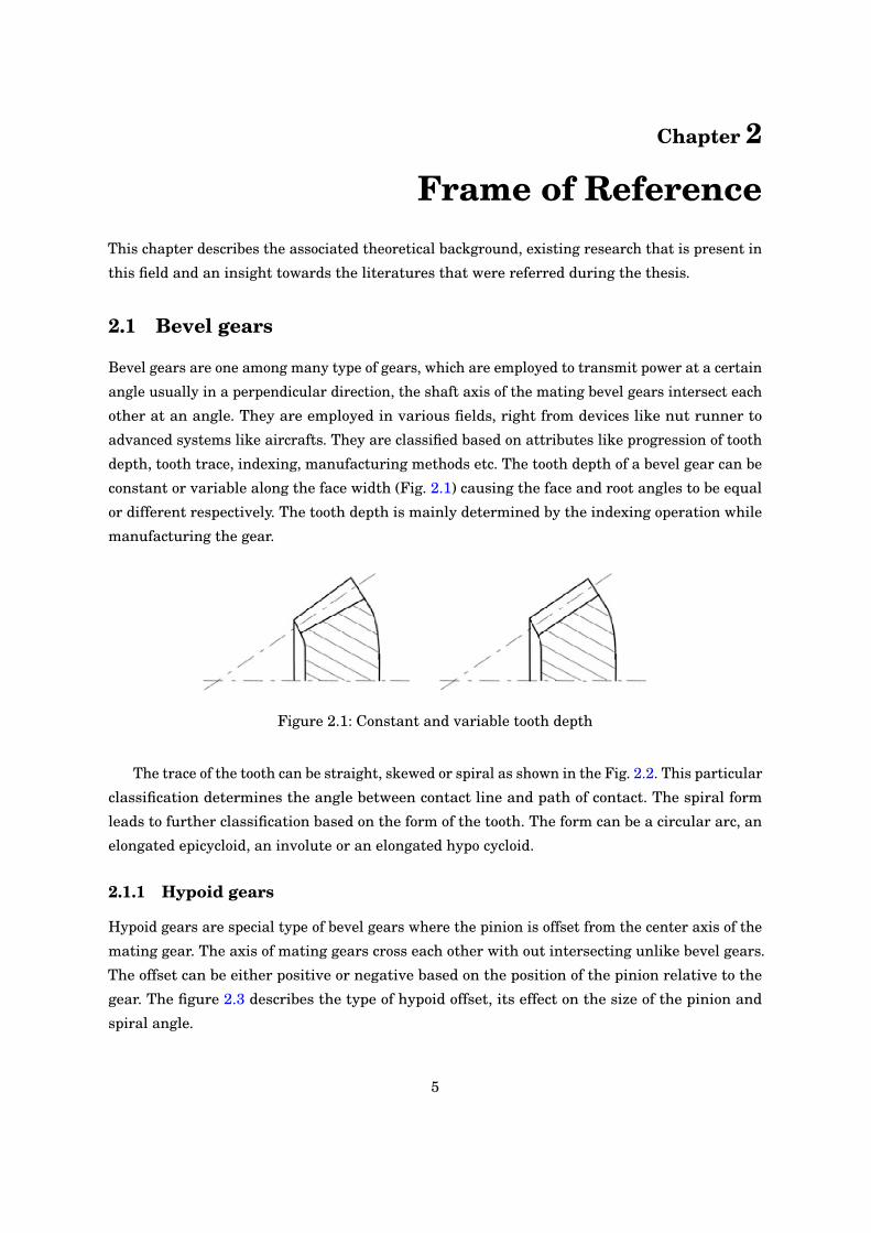
depth, tooth trace, indexing, manufacturing methods etc. The tooth depth of a bevel gear can be

constant or variable along the face width (Fig. 2.1) causing the face and root angles to be equal

or different respectively. The tooth depth is mainly determined by the indexing operation while

manufacturing the gear.

Figure 2.1: Constant and variable tooth depth

The trace of the tooth can be straight, skewed or spiral as shown in the Fig. 2.2. This particular

classification determines the angle between contact line and path of contact. The spiral form

leads to further classification based on the form of the tooth. The form can be a circular arc, an

elongated epicycloid, an involute or an elongated hypo cycloid.

2.1.1 Hypoid gears

Hypoid gears are special type of bevel gears where the pinion is offset from the center axis of the

mating gear. The axis of mating gears cross each other with out intersecting unlike bevel gears.

The offset can be either positive or negative based on the position of the pinion relative to the

gear. The figure 2.3 describes the type of hypoid offset, its effect on the size of the pinion and

spiral angle.

5

CHAPTER 2. FRAME OF REFERENCE

Figure 2.2: Straight, Skewed and Spiral bevel gears

Figure 2.3: Hypoid Offset

There are two types of hypoid pinion offset, positive and negative. In case of positive offset,

the pinion axis is displaced in the direction of the spiral angle of the gear and in case of negative

the displacement is in the opposite direction of the spiral angle. The mean helix angle of the

pinion when compared with that of the gear is larger for positive offset and smaller for negative

offset. The diameter of the pinion when compared with that of an equivalent gear set with no

offset, increases with positive offset and decreases with negative offset [Klingelnberg, 2016].

6

2.1. BEVEL GEARS

2.1.2 Contact Ratio

Contact ratio is a parameter which describes the average no. of teeth that are simultaneously

engaged. The total contact ratio is the sum of contact ratio and overlap ratio which results

from the working height of the profile and spiral angle respectively, provided the tooth flanks

are perfectly conjugate. Crowning of bevel gears results in slight decrease of the contact ratio

from non crowned gears. Tooth flexibility, contact pattern, flattening of tooth under load, axes

deflection have to be considered while calculating the actual contact ratio.

(2.1) Prof ile contact ratio = εα = Path of contactBase pitch

(2.2) Overlap ratio = εβ = included angle of the f ace width (φβ)included angle of one axial pitch (τ)

(2.3) Total contact ratio = εγ = εα + εβ (valid f or con jugate tooth f lanks)

(2.4) Total contact ratio = εγ =√ε2α +ε2

β) (valid f or ell iptical contact pattern)

Figure 2.4: Contact Ratio source: [Klingelnberg, 2016]

2.1.3 Tooth Force on Hypoid Gears

The contact between hypoid gear pair generates a 3D force which is resolved into three mutually

perpendicular directions namely axial, radial and tangential with respect to the rotation axis of

gear bodies as shown in the fig 2.5. The force value differs depending on the drive or coast side,

the drive flank for pinion is concave and coast flank is convex, whereas for ring gear it is vice

versa.

7


Figure 2.5: Tooth forces. 1 pinion, 2 wheel, 3 direction of rotation, Source: [Klingelnberg, 2016]

2.2 Gear Mesh Stiffness

The compliance involved in an hypoid geared rotor model is a combined effect of many factors. The

major contribution to this is; from the gear and pinion shaft torsional stiffness, three translation

and two rotational stiffness at every bearing location and finally the gear mesh stiffness. The

figure 2.6 shows the lumped mass model of an hypoid gear rotor system.

Figure 2.6: 14 DOF hypoid geared rotor system model, Source [Wang u.a., 2013]

8

2.3. TRANSMISSION ERROR

Gear mesh stiffness is the combined effect of tooth and contact compliance. The hypoid gear

pair usually have three tooth pair contact as shown in the figure 2.7 and this is dependent on load,

pinion roll angle and tooth geometry [Wang u.a., 2013]. Gear mesh stiffness is simply defined as

follows:

(2.5) Km = FeL − eo

where,

Km = mesh stiffness of the gear pair,

F = total force along the line of action in the contact region,

e l and eo are translational loaded and unloaded transmission error (TE).

Figure 2.7: Tooth pair contact regions

The mesh stiffness varies along the gear tooth width, the variation profile is different for each

engaging gear tooth pair, which is the main reason for varying mesh force that cause TE and

vibration in the structure.

2.3 Transmission error

The transmission error (TE) in a gear drive is one of the main reason for gear noise and is termed

as the potential excitation source of vibration in the system [Henriksson.M, 2009]. The vibration

frequency from TE varies from low meshing order frequency to high frequency tonal noise due to

gear tooth surface characteristics.

The TE is defined as the difference between the theoretical angular position of a driven gear

assuming ideal conditions and it’s actual angular position, as shown in the figure 2.8. Mathemati-

cally it is expressed as follows:

(2.6) T.E =Θgear −Rpinion

RgearΘpinion

9


where,

Θgear = angular position of ring gear

Θpinion = angular position of pinion

Rpinion and Rgear = pitch circle radius of pinion and gear respectively.

Figure 2.8: Transmission Error

To study TE in detail, it is classified into three types mainly based on the response at different

torque and speed levels.

1. Geometrical Transmission Error:The Geometrical TE is something which is related to manufacturing defects and assembly

errors in the gear drive unit, a slight eccentricity in the pinion or gear, surface defects

on the flanks, pitch errors etc. are some typical examples which cause geometrical TE. It

is measured by giving a low rotational speed to the pinion with no load/torque so as to

determine the load independent errors in the drive.

2. Static Transmission Error:The Static TE includes all entities which cause geometric TE and in addition to that it also

considers the effect of gear body distortion and gear tooth stiffness into account. Static

TE is measured at low rpm but in loaded condition to capture the effect of varying mesh

stiffness.

3. Dynamic Transmission Error:The Dynamic TE includes all the factors that cause static TE and in addition to that it also

10

2.4. CONTACT MECHANICS

considers the support stiffness, drive shaft stiffness and damping effects from them. In

other words, it tries to take into account the induced disturbance from the support/bearings

due to gear contact. This is measured at high speed and high load rating.

2.4 Contact mechanics

The Hertzian contact mechanics was used to calculate the approximate contact stiffness between

Pinion and Ring gear. Since the contacting bodies were three dimensional, formulations of

elliptical contact [Johnson, 1985] were employed to calculate the contact stiffness between them.

(2.7) Rc =√

RaRb

(2.8) Ra = 1(A+B)− (B− A)

(2.9) Rb =1

(A+B)− (B− A)

(2.10) A+B = 12

{ 1R1xx

+ 1R1yy

+ 1R2xx

+ 1R2yy

}

(2.11) B− A = 12

{( 1R1xx

− 1R1yy

)2 + ( 1R2xx

− 1R2yy

)2 +2( 1R1xx

− 1R1yy

)( 1R2xx

− 1R2yy

)cos(2α)

} 12

(2.12) c =(3PRc

4Ec

) 13 F1

(2.13) F1= 1−[(Ra

Rb

)0.0602 −1]1.456

(2.14) F2= 1−[(Ra

Rb

)0.0684 −1]1.531

Normal stiffness is defined as:

(2.15) k = 2 Ec cF1 F2

where,

R1xx, R1yy, R2xx, R2yy are radius of curvature of two contacting 3D bodies in two mutually

perpendicular planes, the subscript 1 and 2 represent first and second body.

P is the normal load.

’α’ is the angle between orthogonal system of first body w.r.t that of second body.

11


2.4.1 Contact Force in MSC ADAMS

The contact definition in MSC ADAMS between two bodies can be modelled as restitution based

or IMPACT function based. Restitution based contact definition does not support contact between

flexible bodies, where as IMPACT function does.

The IMPACT function in ADAMS is defined as IMPACT (x, x’, x1, k, e, Cmax, d) [MSC-Software,

2017]. The arguments are defined as follows:

x = instantaneous distance between I and J marker of contacting bodies as shown in fig. 2.9

x’= time derivative of the distance between the markers

x1 = distance between I Marker from the boundary of its respective body

k = stiffness of the boundary surface interaction

e = positive real variable that specifies the exponent of the force - deformation characteristic. For

a stiffening spring characteristic, e > 1.0. For a softening spring characteristic, 0 < e < 1.0.

Cmax = damping co efficient

d = specifies boundary penetration which results in full damping from ADAMS Solver

Figure 2.9: Illustration of Impact, Source [MSC-Software, 2017]

(2.16) IMP ACT ={

Max (0, k (x1−x)e−STEP (x, x1−d, cmax, x1, 0). x′)) : x<x10 : x<x1

}The penetration is said to happen only when x < x1 criteria is met and a separating force sets in,

whose value is defined by the Impact function and if x > x1, then the force is set to zero. When

the penetration depth in simulation reaches the set limit ’d’, then there is an activation of full

damping which would have followed a cubic function from 0 to ’Cmax’ as shown in fig. 2.10.

12

2.5. MODAL ANALYSIS

Figure 2.10: Damping co-efficient as function of penetration depth, Source : [MSC-Software, 2017]

2.5 Modal analysis

Modal analysis is a method of identifying the vibration characteristics of a given component in the

form of mode shapes and modal properties such as stiffness and damping. There are two ways to

capture the modal behavior namely, experimental modal analysis and FEM based modal analysis.

The method followed in this thesis is FEM Based Modal Analysis which involves discretizing the

component into finite elements and then capturing its modal behavior within a frequency band of

interest.

FEM Model consist large degree of freedom (DOF) due to large number of nodes in a discretised

component. Hence a technique called FE condensation is used to reduce component’s DOF. Any

condensation technique basically involves creating Ritz vectors that are used to reduce full size

mass, stiffness and damping matrix of a discretized component.

If we consider a system governed by the following equation:

(2.17) Mx′′ + Cx′ + kx = 0

where xT = [x1, x2, x3,.....xn] is the generalized displacement for all n DOF in the model. The

basic idea of FE condensation is to reduce the displacement matrix to ’xr ’ with the help of Ritz

vectors in the following manner:

(2.18) x =Wxr

(2.19) Mr = WT M W , Cr = WT C W , and Kr = WT K W

where, W is the Ritz vector that constitute reduced basis and Mr,Cr,Kr are reduced mass, damp-

ing, and stiffness matrices [Sellgren, 2003]. Some of the important FE condensation techniques

are mentioned below

13


1. Static condensation also termed as Guyan reduction -The technique behind this condensation is to separate the entire DOF as master DOF and

slave DOF, the master DOF are retained where as the slave ones are removed and are

dependent on master DOF. The system is divided as follows:

(2.20)[

Kmm KmsKsm Kss

][umus

]=

[FmFs

]where, K, u, F represents stiffness, displacement and force respectively while subscript ’m’

and ’s’ stands for master and slave DOF. The Ritz vector for this condensation method is

defined as:

(2.21) W =[

I−K−ss1 Ksm

]this is used to reduce the stiffness and mass matrices. Some assumptions in this method

are, for low frequency modes the inertia forces on slave nodes are less significant when

compared with elastic forces exerted by master nodes. Slave nodes move quasi-statically

w.r.t master nodes. The challenges faced in this method are, to match the centre of mass

of reduced model with the parent model and also the inertia properties are affected. An

error called condensation error is introduced, which is dependent on choosing the master

nodes while FEM algorithms try to minimize this error by iteratively choosing different set

of master DOF [Sellgren, 2003].

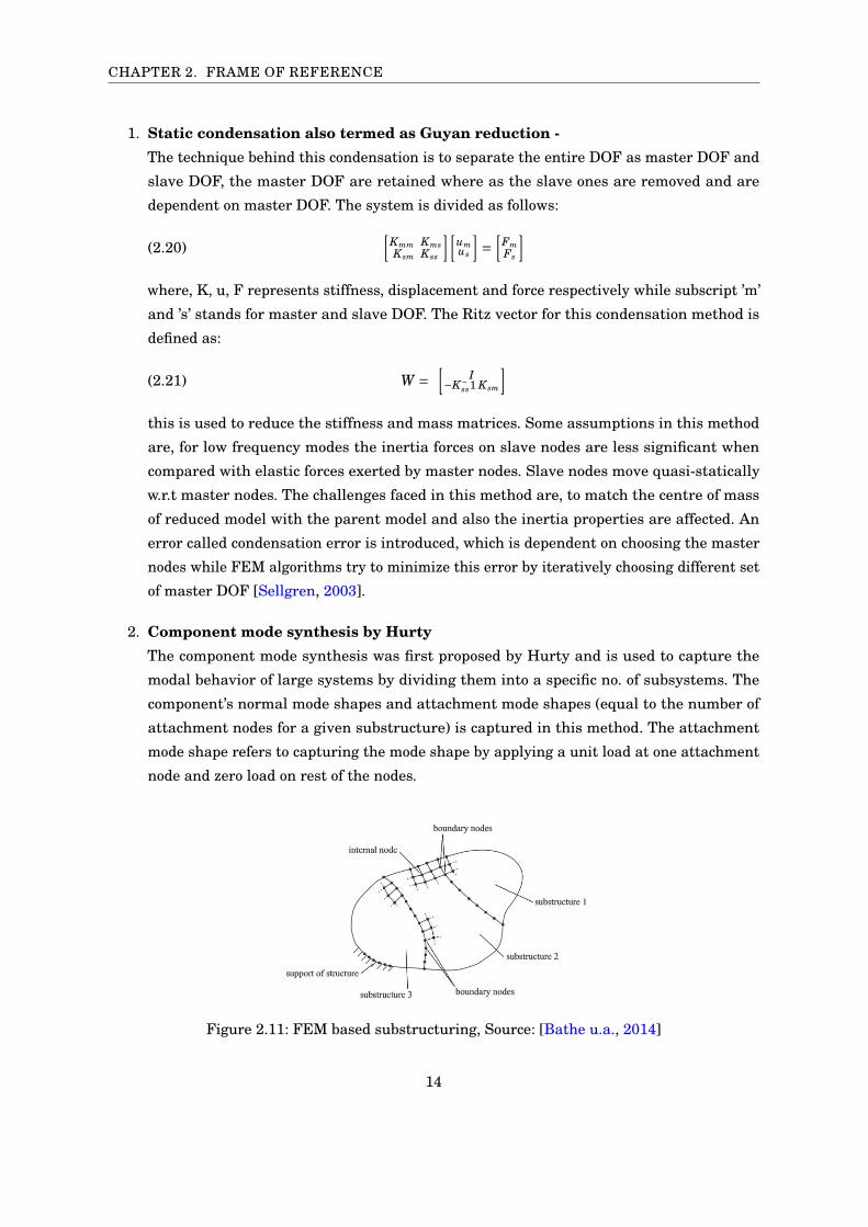
2. Component mode synthesis by HurtyThe component mode synthesis was first proposed by Hurty and is used to capture the

modal behavior of large systems by dividing them into a specific no. of subsystems. The

component’s normal mode shapes and attachment mode shapes (equal to the number of

attachment nodes for a given substructure) is captured in this method. The attachment

mode shape refers to capturing the mode shape by applying a unit load at one attachment

node and zero load on rest of the nodes.

Figure 2.11: FEM based substructuring, Source: [Bathe u.a., 2014]

14

2.5. MODAL ANALYSIS

3. Craig-Bampton MethodThe Craig Bampton method is widely used in CMS technique, this method captures the

constrained mode shapes and fixed interface mode shapes of any given component [Craig,

2011]. The component nodes are subdivided into attachment nodes and internal nodes

fig 2.11, all attachment nodes are fixed during capturing the fixed interface mode shapes

where as in constraint mode shapes, a unit displacement is given to one attachment node

by fixing the rest of them. Hence the relation between the physical co-ordinates and modes

that are synthesised with Craig Bampton method goes as follows:

(2.22) u ={

uBuI

}=

[I 0

φIC φIN

] {qCqN

}Where,

uB = boundary or attachment DOF

uI = interior DOF

φIC = physical displacements of interior nodes in constraint modes

φIN = physical displacements of interior nodes in Normal modes

qC = the modal coordinates of the constraint modes

qN = the modal coordinates of the fixed-boundary normal modes.

Although Craig Bampton method is powerful in synthesizing the modal behaviour some

modifications and considerations are necessary namely, the rigid body mode shapes will

be truncated since MSC ADAMS compute its own rigid body modes, the constraint mode

shapes is based on static condensation and thus lack dynamic content that they should

exhibit [MSC-Software, 2017].

2.5.1 Modal superposition

The dynamic behavior of a finite element model with N DOF can be represented with relatively

less no of mode shapes that are captured from modal reduction techniques, any deformation of a

structure can be represented as combined contributions from these mode shapes. This is termed

as modal superposition and is defined as follows:

(2.23) u =M∑

i=0φi qi

where,

u = physical co ordinates

M = total number of modes

φi = mode shape vector

qi = modal co ordinates

15


2.6 Multi-Body Dynamics

2.6.1 Rigid Body Dynamics

The rigid body dynamics is a simplified form of simulating dynamics, this treats all bodies involved

in the analysis as un-deformable entities, this form of analysis is mainly used in applications

where elastic deformations and modal behavior of structures are of less important.

2.6.2 Flexible Body Dynamics

The flexible body dynamics considers the inherent elastic nature of a component that is involved

in the model, this consideration is important for modelling a complex system whose performance

and reliability assessment is of high importance. There is a huge variation in dynamic force

calculation with and with out considering the elastic nature of a particular component.

2.6.2.1 Kinematics of markers on flexible bodies

In MSC ADAMS, markers play an important role in defining the position, orientation of a flexible

body. They are used to measure entities such as velocity, accelerations of a node on a flexible body

and to define constraints between two bodies.

The instantaneous position of a marker on a flexible body is expressed as follows:

(2.24) ~rp = ~x + ~sp + ~up

where,

~x = position vector from ground to local reference of body B

~sp = undeformed position of point P w.r.t local reference of body B

~up = translational deformation vector of point P from undeformed position P

Figure 2.12: Marker position on a flexible body, Source: [MSC-Software, 2017]

16

2.6. MULTI-BODY DYNAMICS

The above equation is transformed to global coordinates in the following equation:

(2.25) ~rp = ~x + ABG (~sp + ~up)

where,

ABG = is the transformation matrix from local reference frame to gobal reference frame

up is the translation deformation vector of point P which is nothing but the modal superposition

of truncated mode shapes as a result of modal reduction and is expressed as follows:

(2.26) up =Φpq

where,

Φp is a part of complete modal matrix and contains the modal contribution of that node.

q is the modal coordinates

The general co ordinates that governs a flexible body is given as follows:

(2.27) ζ =

x

y

z

Ψ

Θ

Φ

qi

where x, y, z are translational co ordinates, Ψ, Θ, Φ are rotational co ordinates and q is modal

coordinates.

2.6.3 Equations governing flexible bodies

The Lagrange’s equation is applied to govern the flexible bodies and is defined as follows:

(2.28)ddt

(∂L∂ζ

)− ∂L

∂ζ+ ∂F

∂ζ+

[∂Ψ∂ζ

]Tλ − Q = 0

(2.29) Ψ = 0

where,

L = the lagrangian defined as L = T - V,

T being the kinetic energy and V being potential energy of the system.

F = energy dissipation function

Ψ = constraint equations

λ = the lagrange multipliers for constraints

17


ζ = the generalised coordinates

Q = generalised applied forces

Kinetic energy, T is defined as:

(2.30) T = 12ζT M(ζ) ζ

The mass matrix M is governed by nine inertia invariants which are basically computed from

finite number of nodes in the FEM model based on nodal mass, its undeformed location and its

involvement in the component modes Φp [MSC-Software, 2017]

The nine inertia invariants play an important role in the modal formulation of flexible bodies,

by activating only specific invariants the formulation method can be chosen. The four major

formulations are rigid, constant, partial coupling and full coupling.

In ’rigid’ formulation, invariant 6 also termed as modal mass, is disabled. This formulation treats

flexible bodies as rigid and is close to simulating rigid body dynamics. The ’constant’ formulation

disables 3, 4, 5, 8 and 9 invariants, the flexible nature of bodies is included but this formulation

does not take into account the variation of inertial properties due to body deformation.

In case of ’partial’ coupling, invariants 3, 4, 5 and 9 are disabled, this formulation considers

the effect of body deformations on inertial properties. The ’full coupling’ method activates all

invariants except 3 and 4, which results in considering second order correction to the inertial

properties due to body deformations, this is used only when full accuracy is required. There would

be a small difference in the accuracy of results when full coupling method is preferred over partial

but there should always be a fair judgment before choosing between these two methods since

the second order correction might not be required untill and unless the bodies are too flexible or

application demands it.

2.7 Power Transfer Unit

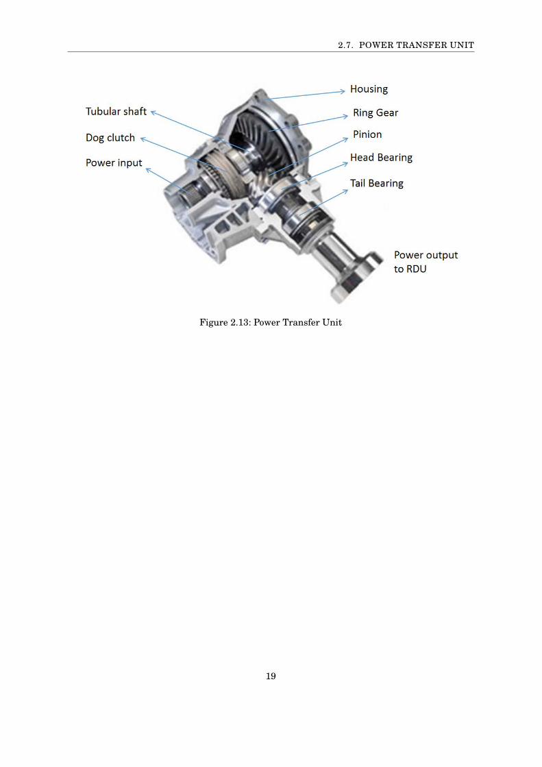
Power transfer unit is the device which will be modelled in this thesis and a brief explanation

about the functionality of this device is given here, see fig. 2.13

Power transfer unit is a device that is installed in AWD vehicle Driveline to control the power

supply to the rear drive unit. The control unit makes decision as to when the power needs

to supplied to the RDU. The power input to PTU is from the transmission unit, clutch plays

an important role in transferring this power to tubular shaft when it is engaged. The power

then flows to ring gear, pinion and finally to RDU via prop shaft. The head and tail bearing

supports pinion inside the housing similarly the tubular shaft is supported by two bearings. All

the components except clutch is modelled in MSC ADAMS which is discussed in the next chapter.

18

2.7. POWER TRANSFER UNIT

Figure 2.13: Power Transfer Unit

19

Chapter 3

ImplementationThis chapter explains the procedure followed in modeling a system within MBS environment and

also the method to perform a co-simulation with a control tool in order to enhance the efficiency

in simulating the dynamic behavior of a system.

3.1 Modeling Procedure

3.1.1 Geometry and Material Properties

Geometry files of all components were analyzed to simplify the features. Splines, threads, center-

ing holes and logos were removed from the geometry in order to reduce the processing time and

computational time of the simulation. These features do not contribute to the accuracy of results

unless they were specifically considered to be important in the analysis.

The properties such as Young’s modulus, poisson’s ratio and density of the material of all compo-

nents were identified in order to be defined while performing the modal analysis.

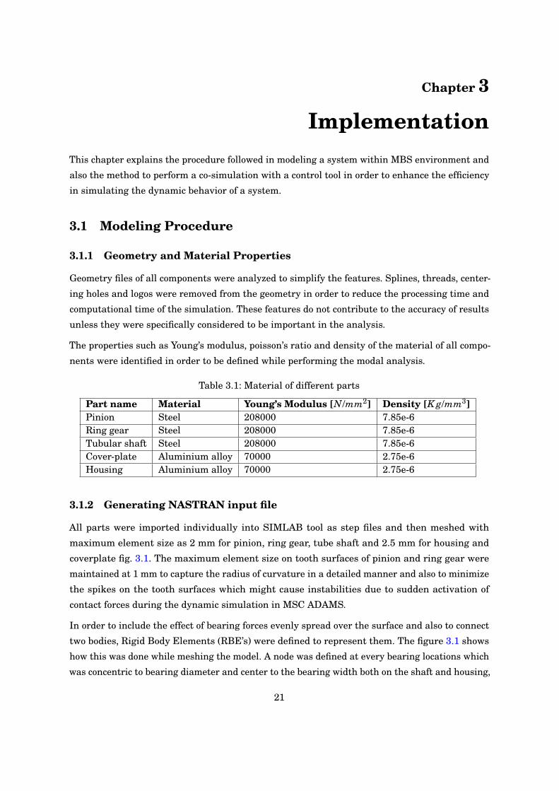
Table 3.1: Material of different parts

Part name Material Young’s Modulus [N/mm2] Density [K g/mm3]Pinion Steel 208000 7.85e-6Ring gear Steel 208000 7.85e-6Tubular shaft Steel 208000 7.85e-6Cover-plate Aluminium alloy 70000 2.75e-6Housing Aluminium alloy 70000 2.75e-6

3.1.2 Generating NASTRAN input file

All parts were imported individually into SIMLAB tool as step files and then meshed with

maximum element size as 2 mm for pinion, ring gear, tube shaft and 2.5 mm for housing and

coverplate fig. 3.1. The maximum element size on tooth surfaces of pinion and ring gear were

maintained at 1 mm to capture the radius of curvature in a detailed manner and also to minimize

the spikes on the tooth surfaces which might cause instabilities due to sudden activation of

contact forces during the dynamic simulation in MSC ADAMS.

In order to include the effect of bearing forces evenly spread over the surface and also to connect

two bodies, Rigid Body Elements (RBE’s) were defined to represent them. The figure 3.1 shows

how this was done while meshing the model. A node was defined at every bearing locations which

was concentric to bearing diameter and center to the bearing width both on the shaft and housing,

21

CHAPTER 3. IMPLEMENTATION

then the surface nodes which comes in contact with the race ways of the bearing were selected

and RBE’s were connected to the centre node and selected surface nodes which results in the form

of a spider net. A similar approach was followed for bolt modelling which is explained in detail

under bolt modelling section 3.2.6. The meshed components were then exported as NASTRAN

input files to perform Modal analysis in NASTRAN-PATRAN.

Figure 3.1: Pinion, Tubular shaft, Ring gear, Housing and Cover-plate

22

3.2. MBS ENVIRONMENT - MSC ADAMS

3.1.3 Generating Modal Neutral File

The NASTRAN input files were imported into PATRAN individually, attachment node set for

each of them was defined for "component mode synthesis" as per Craig-Bampton method. For

this, NASTRAN specific commands called ’QSET’ and ’ASET’ were used in order to define the

attachment node set and the constraints on their DOF respectively. The first 20 modes excluding

the rigid body modes of every individual components were captured.

MSC ADAMS understands the flexible behavior of components in the form of dynamic submodel

from CMS as Modal Neutral File (MNF), prior to performing the modal analysis in PATRAN the

output file format was set to MNF in which the modal behavior of a component was stored as

Craig Bampton Modes.

3.2 MBS Environment - MSC ADAMS

3.2.1 Importing Flexible body in ADAMS

All components in the form of MNF were imported into ADAMS, by doing so, ADAMS automati-

cally detects and removes the rigid body modes of the components and takes only the flexible

modes into account. The "Partial" inertia coupling method in ADAMS was used to represent the

flexible bodies, more information about the coupling methods can be seen under 2.6.3 and the

default mode for damping was applied which means the damping was 1%, 10%, 100% of critical

damping for modes of frequency <100Hz, 100 to 1000Hz and >1000Hz respectively.

3.2.2 Unit system

The unit system that was followed through out the modeling and simulation procedure was

MMKS with length in millimeter, mass in kilogram and time in second.

3.2.3 Joints

The constraints between parts were defined in ADAMS with the help of joints, in this case there

were four rotary joints; two between pinion-housing and two between tubular shaft - housing as

shown in the figure 3.2, there were bolt joints between coverplate - housing, housing - ground,

and coverplate - ground.

The head bearing and tail bearing were located in housing where as the ’B22’ bearing was located

in coverplate and ’B21’ bearing was located inside the housing. The Ring gear was rigidly fixed

to the tubular shaft which was done by joining the RBE spider center node of ring gear with

that of tubular shaft. The housing and coverplate connection is explained in the bolt modelling

procedure section 3.2.6

23


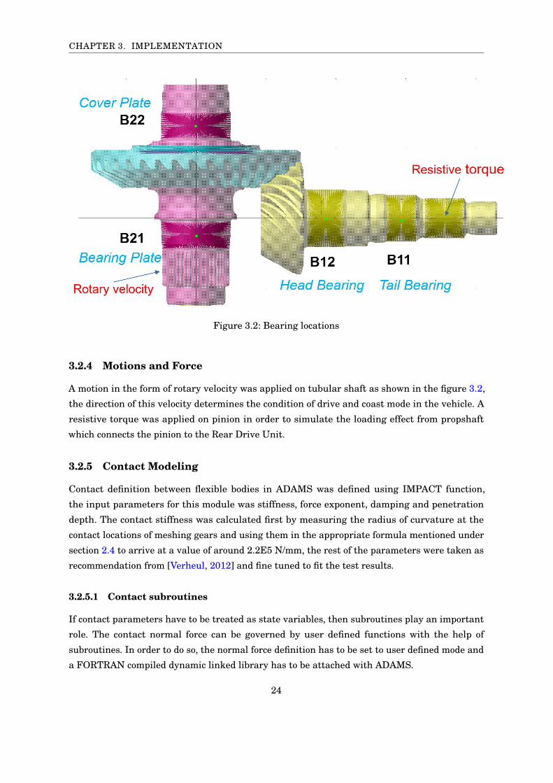
Figure 3.2: Bearing locations

3.2.4 Motions and Force

A motion in the form of rotary velocity was applied on tubular shaft as shown in the figure 3.2,

the direction of this velocity determines the condition of drive and coast mode in the vehicle. A

resistive torque was applied on pinion in order to simulate the loading effect from propshaft

which connects the pinion to the Rear Drive Unit.

3.2.5 Contact Modeling

Contact definition between flexible bodies in ADAMS was defined using IMPACT function,

the input parameters for this module was stiffness, force exponent, damping and penetration

depth. The contact stiffness was calculated first by measuring the radius of curvature at the

contact locations of meshing gears and using them in the appropriate formula mentioned under

section 2.4 to arrive at a value of around 2.2E5 N/mm, the rest of the parameters were taken as

recommendation from [Verheul, 2012] and fine tuned to fit the test results.

3.2.5.1 Contact subroutines

If contact parameters have to be treated as state variables, then subroutines play an important

role. The contact normal force can be governed by user defined functions with the help of

subroutines. In order to do so, the normal force definition has to be set to user defined mode and

a FORTRAN compiled dynamic linked library has to be attached with ADAMS.

24


Figure 3.3: Contact definition

The CNF subroutine allows to control the contact parameters such as stiffness, force exponent,

damping and penetration depth. The CFF subroutine helps to control the contact frictional

parameters. Although, a simulation was set up to vary the contact stiffness dynamically based on

the variation of surface characteristics on tooth flank, it took significantly more time to solve and

accuracy of result was affected.

The reason behind this was, MSC ADAMS has to continuously exchange data with .dll file in

order to generate the normal force and apart from that, the automatic intermediate steps to

compute normal force when the contact is detected was lacking while using subroutines which

demands the simulation error tolerance to be set to a lower value.

3.2.6 Bolt modeling

Bolt stiffness has significant effect on the behavior of a system, which means there is a difference

in the dynamic response with two mounting points fixed together and the dynamic response with

a stiffness definition between them. In this model there were 15 bolts used to hold the entire

assembly in place, the table 3.2 shows the bodies that were coupled together with these bolts.

The tubular shaft was supported by two bearings, one bearing was located inside the housing and

the other one was located in the Cover plate, which makes it important to define bolt stiffness

between these two bodies.

25


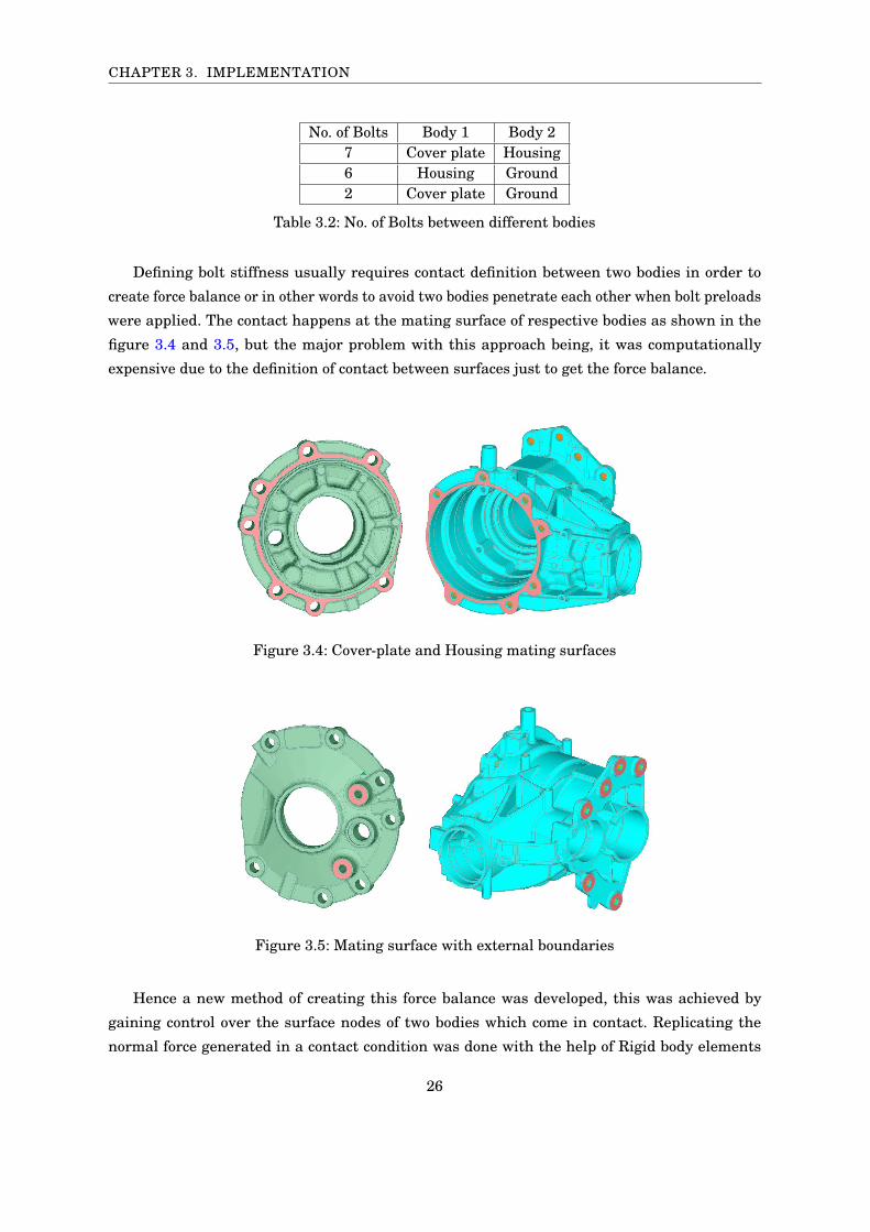
No. of Bolts Body 1 Body 27 Cover plate Housing6 Housing Ground2 Cover plate Ground

Table 3.2: No. of Bolts between different bodies

Defining bolt stiffness usually requires contact definition between two bodies in order to

create force balance or in other words to avoid two bodies penetrate each other when bolt preloads

were applied. The contact happens at the mating surface of respective bodies as shown in the

figure 3.4 and 3.5, but the major problem with this approach being, it was computationally

expensive due to the definition of contact between surfaces just to get the force balance.

Figure 3.4: Cover-plate and Housing mating surfaces

Figure 3.5: Mating surface with external boundaries

Hence a new method of creating this force balance was developed, this was achieved by

gaining control over the surface nodes of two bodies which come in contact. Replicating the

normal force generated in a contact condition was done with the help of Rigid body elements

26


(RBE) as shown in the figure 3.9. If we consider a mating surface of a particular body, then RBEs

were defined between the surface nodes of this mating surface and a single node which was away

from the surface by a certain distance. This helps us to gain control over surface nodes through

which we can define boundary conditions.

Figure 3.6: Cover-plate mating surface nodes connected to a single node through RBEs

Figure 3.7: Housing mating surface nodes connected to a single node through RBEs

In this case the mating surface nodes of housing and cover-plate were connected via RBEs to

their respective single node which was at a certain distance from the mating plane, farther this

single node from the mating plane better was the normal force on the contacting bodies. At last

27


both "single nodes" of two contacting bodies were fixed together as shown in the figure 3.8. The

concept of this procedure for a single bolting region is explained in the figure 3.9

Figure 3.8: Two components in place with their single node connected to each other

Figure 3.9: Conceptual representation of a single bolting region

28


All mounting holes have a centre node which was connected by RBEs to the nodes on the

threaded region in case of threaded holes or to the nodes of bolt-head seating surface in case of

clearance holes as shown in the figure 3.10

Figure 3.10: Illustration of connecting two centre nodes with a bolt

3.2.6.1 Bolt stiffness and damping calculation

The bolt stiffness can be approximately calculated with the following formulation:

(3.1) K = AEL

where,

A = Area of cross section of bolt

E = Young’s modulus of the material

29


L = Shank length of the bolt

A rough calculation on the stiffness gives a value of around 5e5 N/mm to 6e5N/mm. To have

an idea on the damping co-efficient of the bolt, it’s mass was calculated which was 20.52g and

assuming 50 percent contribution to the stiffness, a mass of 10g can be considered to calculate

the first natural frequency and an estimate on its damping.

(3.2) Natural f requency, ωn =√

Km

(3.3) CriticalDamping, Cc = 2 m ωn

The structural damping can be around 2 percent of critical damping [Gaul u.a., 2008] and with

that a 0.1 Ns/mm of damping co-efficient can be estimated. Both the calculated stiffness and

damping values were in the agreeable range as mentioned in [Tsai u.a., 1988].

3.2.6.2 Defining Bolt Stiffness in ADAMS

In ADAMS "S-Force" with stiffness and damping characteristics was defined between two center

nodes of a particular mounting region. With this definition the bolt stiffness and damping

properties were taken into account eqn 3.4. Bolt pre-load was incorporated by defining a constant

force value within the "SForce" equation. The equation 3.4 is an illustration of how a bolt was

defined using the two markers of different bodies (two center nodes in this case) which can be

connected via stiffness damping and preload values.

(3.4) Fb = Kb dx + Cdxdt

+ Preload

where,

Fb = bolting force

Kb = bolt stiffness

dx = change in distance between two connected nodes

C = bolt damping co-efficientdxdt = rate of change of distance between two nodes

3.2.6.3 Defining Sensors

Sensors in ADAMS were defined to evaluate and store the value of a particular expression during

a specific instant of time which can be utilized later in the model . In this case defining sensors

was a requirement to model the bolting effect in a proper manner, the main reason being elastic

deformation of the bodies when bolt preload was applied.

30


Figure 3.11: Defining Sensors in ADAMS

Force due to bolt stiffness was generated only when there was a change in the distance

between two connected nodes. As bolt preload was applied during the initial stage of simulation

two connected nodes used to come closer due to the flexible nature of bodies, this created an

unwanted spring force between the two nodes in the opposite direction that reduced the preload

value to some extent. Hence the unwanted spring force was reset to zero by measuring the elastic

deformation of two nodes with the help of sensors and from there on the spring force would be

generated as it should be in reality.

3.2.7 Bearing stiffness

In ADAMS model, bushings were defined in order to include the compliance effect of bearings

at specific locations. The bushing module definition in ADAMS had an option to input 6 DOF

(3 translation and 3 rotation) stiffness and damping properties between two bodies, along with

preload values for each DOF. This makes it convenient to model bearings by defining 5 DOF

31


stiffness and damping properties, setting the rotational axis stiffness and damping to zero as

shown in the figure 3.12.

Figure 3.12: Defining Bushings in ADAMS

The inputs for stiffness values were from a specific tool, which was efficient in estimating

the bearing stiffness for a given load. Although stiffness of the bearing is non linear and load

dependent, a fair approximation should give better results. As explained there were four bearings

in the model, each of them having specific stiffness value depending on their configuration and

type.

3.3 Models built in MSC ADAMS

3.3.1 Hypoid Gear Pair Model

Hypoid gear pair model includes tubular shaft, ring gear and pinion. The main purpose of this

model was to simulate the experimental set up in Gleason 600HTT tester machine, which was

used to measure the transmission error of an hypoid gear set. The boundary conditions were

defined similar to how the components were mounted in the testing machine. The pinion and

tubular shaft were connected to the ground via revolute joint this replicates the conditions of

holding the components in the chuck of the tester machine. A torque was defined on the pinion in

a direction opposite to its rotation so as to generate the resistive load and for the tubular shaft a

specific rotational velocity was defined. This was followed by defining the contact between pinion

and ring gear. The model is shown in the figure 3.13.

32

3.3. MODELS BUILT IN MSC ADAMS

Figure 3.13: Hypoid gear pair model

3.3.2 Complete Model

The complete model includes pinion, ring gear, tubular shaft, housing and cover-plate fig 3.14.

There are four bearings in the real product which were modelled as bushings as explained in

3.2.7. The bolt stiffness was incorporated in the model as explained in 3.2.6.

The contact conditions between Pinion and Ring Gear for complete model were defined as follows:

Stiffness 2e5 N/mmExponent 3Damping 60 Ns/mm

Penetration Depth 0.03 mm

Table 3.3: Contact Parameters

33


Figure 3.14: Complete model of PTU

As explained, the method of bolting the parts together was responsible to hold the structure

intact. But the activation of these bolt preloads and bolt stiffness properties need to be defined

carefully. For example if all the bolt preloads connecting the housing were activated at the same

instant then, it would cause simulation errors due to force convergence problem. So the activation

of bolt preloads were defined as how the product was assembled in reality. The sequence is

34

3.4. SIMULINK-ADAMS CO-SIMULATION

described in the table 3.4.

Table 3.4: Activation Sequence of Bolt Preload

Time (sec) Sequence of Events0 – 0.1 Bolt preload, Cover-plate and Housing0.1 - 0.2 Bolt preload, Housing and Ground0.2 - 0.3 Bolt preload, Cover-plate and Ground0.5 Activation and Evaluation of Sensors0.5 - 0.6 Stiffness definition for all Bolts0.9 - 1 Resistive Torque applied on the pinion

3.3.3 Solver settings and Simulation Parameters

Different solver settings in MSC ADAMS and their capabilities in solving the dynamic equations

of a similar system was studied in [Stefano.Orzi, 2016]. Based on that, solver settings were

chosen as shown in the table 3.5. The solver executable threads were set to 8 which utilizes the

maximum CPU capabilities.

Table 3.5: MSC ADAMS Solver settings

Integrator GSTIFFError tolerance 1e-3

Formulation I3Corrector Original

3.4 SIMULINK-ADAMS Co-simulation

Co-simulation is a technique which involves integrating two or more tools to increase the perfor-

mance and flexibility of a simulation. In this thesis, a co-simulation between MSC ADAMS and

SIMULINK was established in order to explore optimization methods for developing the product

and also creating an option for future to test control strategies. This can be developed to combine

multiple mechanical and electrical systems.

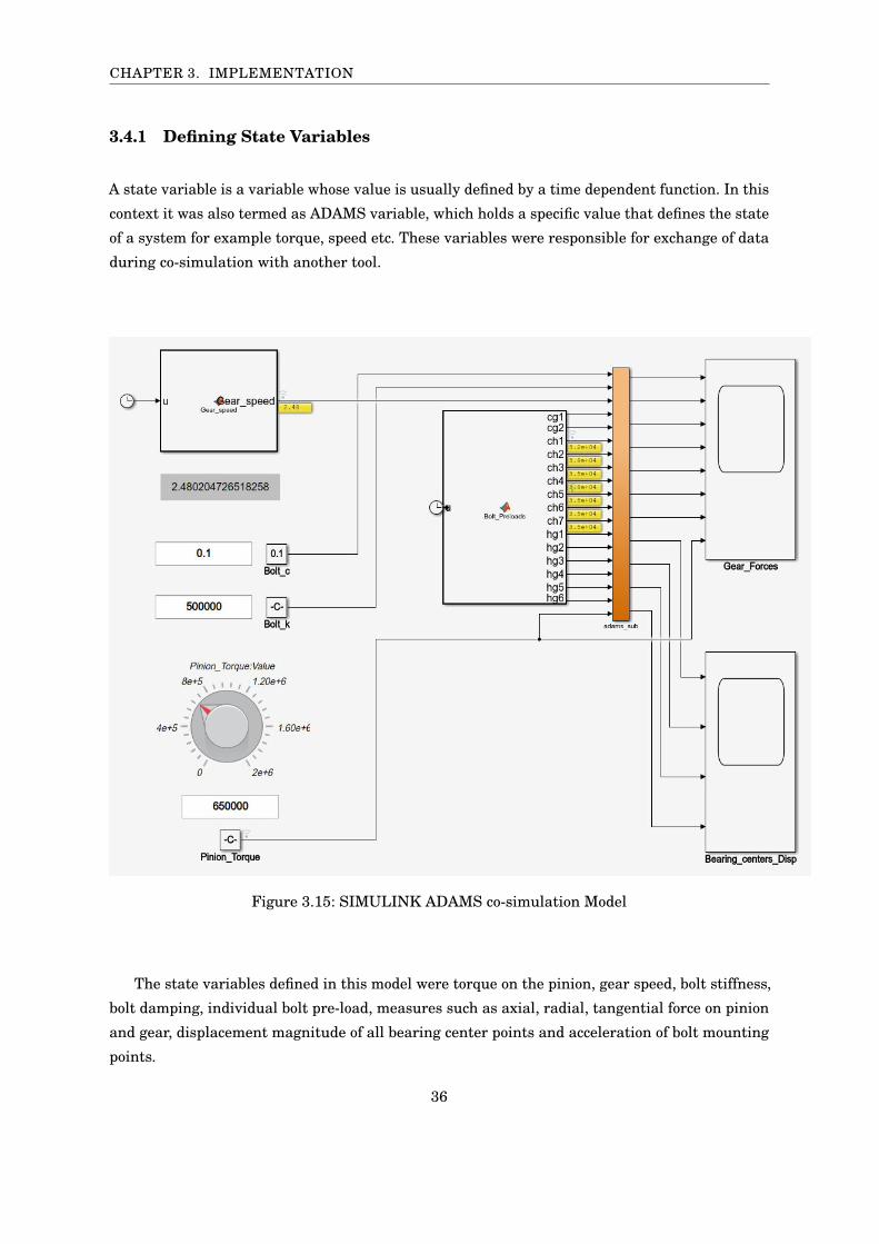
The figure 3.15 shows the co-simulation that was set up. The "adams sub" block represents the

complete model of PTU. An optimization block for bolt preloads was set up in this case. There

were two scopes(graphical window) in this model one with the name Gear force where the forces

on gear bodies were plotted instantaneously as the simulation was running and the other scope

with name Bearing centre disp. showed the plot of bearing point displacement magnitude. The

simulation was basically to set a unique bolt preload values between coverplate and housing

each second and the effect of that on the bearing centre displacement was observed. This was

performed for 57 different combination of bolt preloads as a part of DOE.

35


3.4.1 Defining State Variables

A state variable is a variable whose value is usually defined by a time dependent function. In this

context it was also termed as ADAMS variable, which holds a specific value that defines the state

of a system for example torque, speed etc. These variables were responsible for exchange of data

during co-simulation with another tool.

Figure 3.15: SIMULINK ADAMS co-simulation Model

The state variables defined in this model were torque on the pinion, gear speed, bolt stiffness,

bolt damping, individual bolt pre-load, measures such as axial, radial, tangential force on pinion

and gear, displacement magnitude of all bearing center points and acceleration of bolt mounting

points.

36

3.4. SIMULINK-ADAMS CO-SIMULATION

3.4.2 Exporting ADAMS control Plant

ADAMS control plant export was a step to specify the input and output variables of the ADAMS

system block that will be later used in the co-simulation environment. This step also requires

specifying the target software which in this case was MATLAB. Initialization command can be

used to initialize certain variable value before the start of co-simulation.

3.4.3 Simulation parameters in SIMULINK

An ODE15s (stiff/NDF) solver was used in SIMULINK to perform the co simulation, animation

mode was set to batch and simulation mode being discrete which means the control equations

are solved by SIMULINK and mechanical system equations were solved by ADAMS solver in the

background.

Figure 3.16: SIMULINK Solver settings

37

Chapter 4

Results and DiscussionIn this chapter, the results obtained from the simulation of various models are discussed.

4.1 Forces on Hypoid Gears

4.1.1 Analytical results

The three mutually perpendicular gear body forces namely axial, radial and tangential force that

are acting on the hypoid gear sets can be calculated for any given torque using the analytical

formulae. The same has been calculated for two torque levels i.e. 650Nm and 1343Nm acting on

the pinion which corresponds to 1646.6Nm and 3402.2 Nm on Gear side. The analytical results

are shown in table 4.1 & 4.2.

Table 4.1: Forces acting on Pinion

Torque (Nm) Axial Force (N) Radial Force (N) Tangential Force (N)650 20722 2301 216081343 42941 5093 44540

Table 4.2: Forces acting on Ring gear

Torque (Nm) Axial Force (N) Radial Force (N) Tangential Force (N)1647 659 14531 262683402 1297 30382 54120

4.1.2 MSC ADAMS Simulation results

ADAMS simulation was performed with a pinion torque of 650 Nm maintaining its rotational

speed at 60 rpm. The forces acting on the gear bodies is shown in fig 4.1 to fig 4.6. It is important to

note that the torque was zero till 0.9 sec and was taken to the desired level within the simulation

time frame of 0.9 to 1 sec. As explained before the delay in application of torque was because of

the bolt preload and stiffness activation within simulation time span of 0 to 0.9 second. The blue

dashed line in the below figures represents the analytical value for the same.

The comparison between analytical and simualtion results shows a good correlation of forces

acting on the gear bodies, but still there was an error of some percentage depending on the

magnitude of forces. This can be attributed to the fact that analytical formulae considers a

constant pitch circle diameter which is not the same in reality and also the angle used to resolve

the force components might vary since the tooth surfaces are not smooth enough.

39

CHAPTER 4. RESULTS AND DISCUSSION

Figure 4.1: Pinion Axial Force

Figure 4.2: Pinion Radial Force

Figure 4.3: Pinion Tangential Force

40

4.1. FORCES ON HYPOID GEARS

Figure 4.4: Gear Axial Force

Figure 4.5: Gear Radial Force

Figure 4.6: Gear Tangential Force

41


4.2 Transmission Error (TE)

The TE was computed by measuring the difference between the angular position of pinion

calculated based on ring gear rotation and actual angular position of the marker on the pinion

where resistive torque was applied. The fig 4.7 shows TE signal that was measured from the

simulation with a specific Gear torque and specific Pinion rotational speed. This particular

simulation setting is similar to the End of Line (EOL) test that was performed at the test rig once

the complete product was assembled.

Figure 4.7: Transmission Error (1 to 2 sec)

The interesting part of Fast Fourier transform (FFT) of TE signal is to observe the amplitude of

the signal at the meshing frequency which is defined as the no. of teeth on pinion/gear multiplied

by the base rotational speed of pinion/gear in rps respectively. Since, the pinion had a specific

no. of teeth a certain rotational speed would give us the fundamental frequency also called as

meshing frequency and its first harmonic which is twice the fundamental frequency, typically

major part of the TE disturbance will be concentrated in the base meshing frequency and the

amplitude usually decreases with higher orders and dies out.

In the figure 4.8 it can be seen that the TE at fundamental frequency is around 27.5 micro-radian

and at first harmonics it is around 8 micro-radian. The contact conditions and simulation settings

are mentioned in the table 4.3.

ADAMS Solver GSTIFFError tolerance 1e-3Inertia coupling PartialContact stiffness 2e5 (N/mm)

Exponent 3Damping 60 (Ns/mm)

Penetration depth 0.03 (mm)

Table 4.3: Settings - Simulation and Contact parameters

42

4.2. TRANSMISSION ERROR (TE)

Figure 4.8: FFT of Transmission Error signal (1 to 2 sec)

4.2.1 TE - Hypoid gear set level

This simualtion was performed at a gear set level with pinion, ring gear and tubular shaft. The

settings used for this simulation was same as used for the above full model but, only change was

the torque on the gear. The TE obtanied from the ADAMS simulation is shown in fig 4.9 and fig

4.10.

Figure 4.9: Transmission Error - Hypoid gear set level

Figure 4.10: FFT of TE signal - Hypoid gear set level

43


This simulation was similar to the TE test rig set up. In the figure 4.10 it can be seen that the

TE at fundamental frequency is around 25.17 micro-radian and at first harmonics it is around

8.4 micro-radian, which goes on decreasing at higher orders.

4.2.2 EOL and TE Test Rig - Test results

The End of Line test was carried out in a test rig which measures the TE of the complete

assembled unit at the end of assembly line and the test results are shown in table 4.4. It is

important to note that the TE measured in this test rig is from zero to peak which means its

amplitude is comparable to the amplitude of TE signal in ADAMS simulation.

Frequency [Hz] Test [u-rad] Simulation [u-rad]Fundamental 28 27.5

First harmonic 5 8

Table 4.4: EOL test results

The hypoid gear set level test was carried out in TE tester machine, which was designed to

measure TE of a given hypoid gear pair. The TE measured in this machine was peak to peak

which means 50 percent of its amplitude corresponds to the TE predicted by ADAMS simulation.

The results from the tester machine is shown in table 4.5

Frequency [Hz] Test [u-rad] Simulation [u-rad]Fundamental 26 (13) 25.17

First harmonic 4 (2) 8.4

Table 4.5: TE tester results

4.2.3 Comparing Test and Simulation TE values

The comparison of simulation results with test results shows that the fundamental TE for

complete model is closely matching with test results, where as at first harmonic is slightly

deviating by 3 micro-radian. In case of hypoid gear set level, only 50 percent of test results

(since it is peak to peak) i.e. 13 and 2 micro-radian should be compared with the simulation

results which is not exactly matching, the reason for this could be that the compliance effect of

spindle bearing in tester machine was not included in hypoid gear set model, which is driving the

simulation results higher. More importantly the complete model TE is correlating well with the

test results which is beneficial in many ways.

4.3 Acceleration of Bearing points

The acceleration at bearing points plays an important role in the performance of any drive unit,

lesser the acceleration in those points better it is from NVH perspective, which leads to elongated

44

4.3. ACCELERATION OF BEARING POINTS

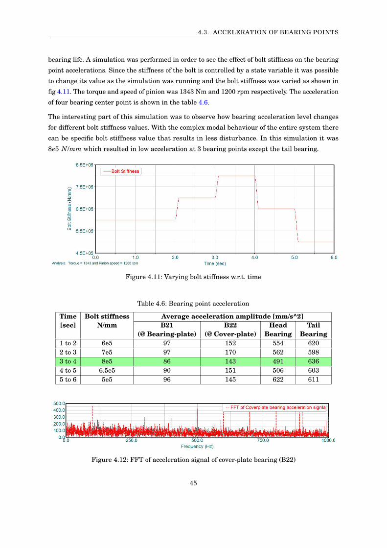
bearing life. A simulation was performed in order to see the effect of bolt stiffness on the bearing

point accelerations. Since the stiffness of the bolt is controlled by a state variable it was possible

to change its value as the simulation was running and the bolt stiffness was varied as shown in

fig 4.11. The torque and speed of pinion was 1343 Nm and 1200 rpm respectively. The acceleration

of four bearing center point is shown in the table 4.6.

The interesting part of this simulation was to observe how bearing acceleration level changes

for different bolt stiffness values. With the complex modal behaviour of the entire system there

can be specific bolt stiffness value that results in less disturbance. In this simulation it was

8e5 N/mm which resulted in low acceleration at 3 bearing points except the tail bearing.

Figure 4.11: Varying bolt stiffness w.r.t. time

Table 4.6: Bearing point acceleration

Time[sec]

Bolt stiffnessN/mm

Average acceleration amplitude [mm/s^2]B21

(@ Bearing-plate)B22

(@ Cover-plate)Head

BearingTail

Bearing1 to 2 6e5 97 152 554 6202 to 3 7e5 97 170 562 5983 to 4 8e5 86 143 491 6364 to 5 6.5e5 90 151 506 6035 to 6 5e5 96 145 622 611

Figure 4.12: FFT of acceleration signal of cover-plate bearing (B22)

45


4.4 Acceleration of mounting points

The results that are important to predict NVH performance of a drive unit are discussed here. Bolt

Acceleration Computation (BAC) and Surface Velocity Levels (SVL) are some of the important

measures to analyse the NVH Performance of a particular system [Selmane u.a., 2004]. These

measures also play an important role in the development of a product for better NVH performance

relative to a reference product.

The bolt joints’ acceleration between cover-plate and housing were analyzed in this case, but

this analysis can be extended to other mounting points in order to improve the complete system.

The bolt joints acceleration results were taken from the same simulation that was performed

in case of bearing point acceleration mentioned in section 4.3. The table 4.7 shows bolt joints’

acceleration between cover-plate and housing. This acceleration has been measured at markers

on the cover-plate to which one end of the bolt was connected.

Table 4.7: Bolt Joint Accelerations

Avg. acceleration amplitude [mm/s^2]Time[sec]

Bolt stiffness[N/mm] CH1 CH2 CH3 CH4 CH5 CH6 CH7

1 to 2 6e5 107 126 139 133 125 79 922 to 3 7e5 134 140 162 161 153 98 1073 to 4 8e5 104 121 140 137 127 76 864 to 5 6.5e5 113 123 149 143 133 82 875 to 6 5e5 109 114 139 143 134 76 78

** CH1 stands for cover plate-housing bolt number 1 and there are seven bolts securing

coverplate to housing, hence CH1 to CH7

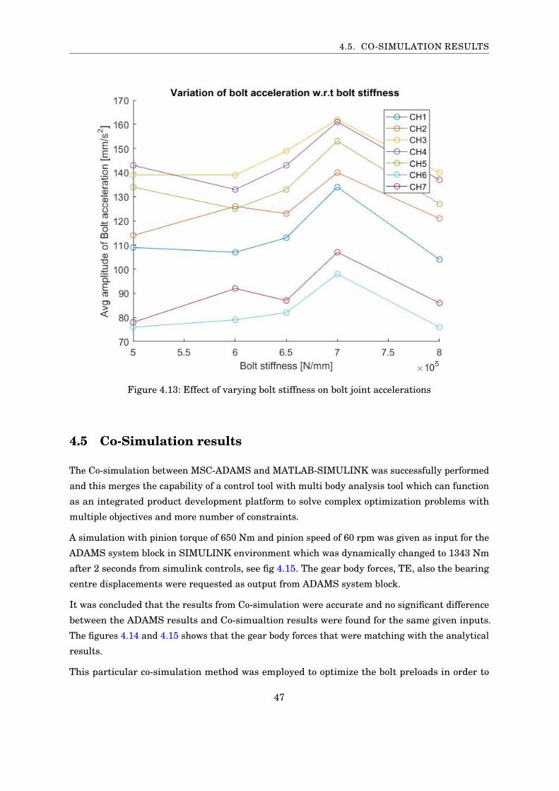
From the table 4.7 it can be clearly concluded that average acceleration values were affected

by varying the bolt stiffness and there is no direct relation as such between them since it is a

combined effect of various stiffness in the system. A specific bolt stiffness value of 8e5 N/mm has

a minimizing effect on the overall acceleration levels in case of bolted joints, although it was not

the lowest level for individual case but was still relatively low fig. 4.13

This method of analysing bolt accelerations and bearing point accelerations definitely has a

potential to tune a specific product for better performance in terms of NVH by just making some

minor modifications to the bolt stiffness value. It would be interesting to analyse the effect of

varying individual bolt stiffness.

The further development in this regard is to analyze the effect of varying bearing preloads, bolt

preloads and the combined effect of these on the NVH performance of the system. Since the

optimisation process becomes complicated to be only handled by ADAMS, a co-simulation might

be a better option.

46

4.5. CO-SIMULATION RESULTS

Figure 4.13: Effect of varying bolt stiffness on bolt joint accelerations

4.5 Co-Simulation results

The Co-simulation between MSC-ADAMS and MATLAB-SIMULINK was successfully performed

and this merges the capability of a control tool with multi body analysis tool which can function

as an integrated product development platform to solve complex optimization problems with

multiple objectives and more number of constraints.

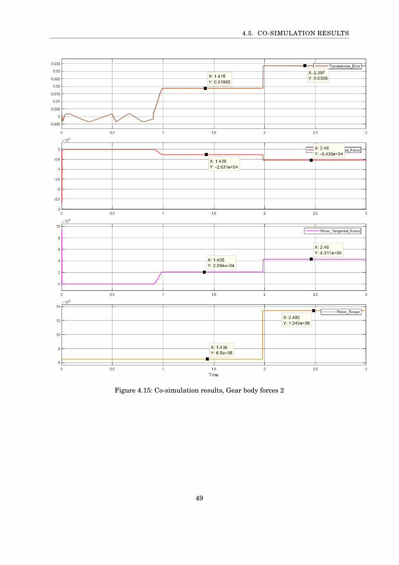
A simulation with pinion torque of 650 Nm and pinion speed of 60 rpm was given as input for the

ADAMS system block in SIMULINK environment which was dynamically changed to 1343 Nm

after 2 seconds from simulink controls, see fig 4.15. The gear body forces, TE, also the bearing

centre displacements were requested as output from ADAMS system block.

It was concluded that the results from Co-simulation were accurate and no significant difference

between the ADAMS results and Co-simualtion results were found for the same given inputs.

The figures 4.14 and 4.15 shows that the gear body forces that were matching with the analytical

results.

This particular co-simulation method was employed to optimize the bolt preloads in order to

47


minimise the displacement of bearing centers. A DOE was setup to change the bolt preloads

between cover-plate and housing from a nominal value of 3.5e4 by a value of +2e3 and-2e3 as two

levels. Therefore for every second the seven bolts between coverplate and housing had a unique

preload value differing slightly from the nominal value. It can be seen in the figure 4.16 that,

even though the variation in bolt preloads had an effect on the bearing point displacement it

was negligibly small i.e. less than 1 micron difference between each trial every second and hence

it was concluded that a different criteria has to be followed to optimize bolt preloads such as

comparing bearing point accelerations instead of bearing point displacement.

Figure 4.14: Co-simulation results, Gear body forces 1

48

4.5. CO-SIMULATION RESULTS

Figure 4.15: Co-simulation results, Gear body forces 2

49


Figure 4.16: Effect of varying bolt preloads on Bearing center displacement, x-axis representssimulation time in seconds and y axis represents the displacement magnitude from global originin mm

4.6 Transient behavior of the system

A simulation of the complete model was performed with a constant pinion torque of 1343 Nm,

varying pinion speed from 0 to 4800 rpm in 0 to 10 sec duration to understand the transient

dynamic behavior of the system. Bearing point accelerations were studied to understand the

transient behavior of the system.

3D fft were plotted as we can analyze the effect of varying pinion speed and also at different time

slice. In figures 4.17 and 4.18, x axis represents frequency content of the variation in a particular

50

4.6. TRANSIENT BEHAVIOR OF THE SYSTEM

entity for example acceleration in bearing B21, y axis represents time slice and z axis represents

the amplitude of signal. Since the torque is not varied the nominal force acting on the gear bodies

remains the same and only power in the drive increases as the simulation time progress.

Figure 4.17: 3D FFT of Bearing B21 acceleration

Figure 4.18: 3D FFT of Bearing B22 acceleration

51


Figure 4.17 and 4.18 shows the variation of bearing point acceleration amplitude with respect

to pinon speed. It can be seen that the acceleration levels are lower at initial stages and higher in

the time range of 7 to 10 seconds since it corresponds to higher power in the drive unit as the

torque is constant and pinion speed is increasing linearly w.r.t time. Due to limitation of time

much analysis could not be made on transient behavior, but can be a potential future work to

study how system responds for sudden change in the inputs.

The deformation plot of the entire model is captured to have a rough idea of what is happening

in the model during the simulation. The figure 4.19 shows the deformation contour, important

areas to observe in this plot are the torque transfer regions gear contact region and bolting region

which gives a visual approximation of the deformation that is happening during the simulation

for a particular torque level.

Figure 4.19: Deformation contour of PTU during simulation

52

Chapter 5

Conclusions and Future workThis chapter mentions the conclusions that were derived from the results and recommends the

possible future work to progress further.

5.1 Conclusions

The thesis was able to model the dynamic behavior of a Power Transfer Unit mounted in an AWD

vehicle, the transmission error predicted by the built model in MSC ADAMS was well within

the agreeable range, the TE of the complete model correlated well with the EOL tests that were

carried out at GKN.

The forces generated on gear bodies for a specific torque during the simulation were matching

with the analytical results, which was an added confirmation that no extremely large force due

to material "dig-in" was happening in the simulation and the model can be effectively used for

further analysis.

A new approach was followed to incorporate bolt stiffness in the model, with which different

studies were carried out by varying the bolt stiffness and analyzing its effect on the acceleration

levels at bearing points and mounting points, since these were crucial from NVH perspective

and used as qualitative measure to predict the performance and durability of a product. Bearing

stiffness and bearing preload were also modelled by using bushing module in MSC ADAMS.

The co-simulation between SIMULINK and ADAMS was set up and this created opportunities

to integrate the capabilities of a control tool with MBS tool in order to create a platform which

can optimize the design space of a model with multiple objectives and complex constraints. The

co-simulation results correlated well with the results obtained from the simulation performed

solely in ADAMS. A co-simulation was performed with different combination of bolt preloads

between cover-plate and housing with a criteria to minimize the bearing point displacement,

although there was an effect of varying bolt preload, it was negligibly small and hence a different

criteria such as bearing point acceleration was recommended to optimise bolt preload.

From this it was concluded that Multi-Body Simulation in ADAMS had potential to predict the

dynamic behavior of a system if all parameters were taken into account. It was also proven that

MBS can be effectively used to optimize the design and this capability can be improved by co

simulating with SIMULINK. Other auxiliary components such as dog clutch and structures can

be attached in co simulation mode which adds flexibility to develop and create complex simulation.

53

CHAPTER 5. CONCLUSIONS AND FUTURE WORK

5.2 Future work

The future work is to incorporate non linearity of bearing stiffness in the model and also to

analyze the effect of varying bearing preloads. Although the transmission error was matching

with EOL test, there was some difference with the hypoid gear set level test which needs to be

understood.

The effect of bolt stiffness on bearing point accelerations and mounting point accelerations needs

to be analyzed in a detail way and should be validated with experimental results. Once it is

accomplished, optimisation could be carried out to find the optimum bolt stiffness and bolt

preloads that meets all the requirement. The new bolt modelling method tried in this thesis has

to be critically evaluated in order to verify its correctness.

The capabilities of ADAMS-SIMULINK co-simulation has to be explored more in order to perform

simulation by coupling auxiliary components such as dog clutch to the main model. Templatizing

the current procedure can be done since that option is available in ADAMS and thus, it can be a

general platform to model similar products with varying designs which will definitely save time.

54

ReferencesTsai, J. S. / Chou, Y. F.(1988): The identification of dynamic characteristics of a single bolt joint, 3:

487–502.

Sellgren, Ulf(2003): COMPONENT MODE SYNTHESIS -A method for efficient dynamic simula-

tion of complex technical systems.

Selmane, Abbas / Felice, Mario / Li, Yingmin(2004): Engine Cylinder Blocks and Heads NVH

Improvements: Bolt Accelerations Computation Methodology.

Gaul, L. / Roseira, J. / Becker, J.(2008): Structural Damping with Friction Beams, 3-4: .

Henriksson.M(2009): On Noise Generation and Dynamic Transmission Error of Gears, PhD

dissertation.

Verheul, Chris(2012): ADAMS methodology for contact modelling.

Wang, Yawen / Lim, Teik / Yang, Junyi(2013): Multi-Point Mesh Modeling and Nonlinear Multi-

Body Dynamics of Hypoid Geared SystemIn: SAE International Journal of Passenger Cars -

Mechanical Systems1127-1132.

Bathe, Klaus Jürgen / Dong, Jian(2014): Component mode synthesis with subspace iterations for

controlled accuracy of frequency and mode shape solutions28 - 32.

Jinli, Xu / Lei, Wan / Wenxin, Luo(2016): Influence of Bearing Stiffness on the Nonlinear Dynamics

of a Shaft-Final Drive System14.

Stefano.Orzi(2016): NVH performance prediction in a Rear Drive Unit.

MSC Software(2017): MSC ADAMS 2017, A Reference Manual, MSC Software.

Craig, Roy R.; Kurdila Andrew J. (2011): Fundamentals of Structural Dynamics. , Wiley.

Johnson, K. L. (1985): Contact Mechanics. , Cambridge University Press.

Klingelnberg, Jan (2016): Bevel Gear: Fundamentals and Applications. Berlin, Heidelberg,

Springer Berlin Heidelberg.

Menday, M. (2010): An introduction to noise and vibration issues in the automotive drivetrain

and the role of tribology. In: Rahnejat, Homer (Hg.), Tribology and Dynamics of Engine and

Powertrain.Woodhead Publishing: 663 - 679.

55

Appendix

Figure 1: Deformation at bolting regions

Figure 2: Coverplate - Housing Bolt acceleration, Bolt stiffness 6e5

57

APPENDIX

Figure 3: Coverplate - Housing Bolt acceleration, Bolt stiffness 7e5

Figure 4: 3D FFT of Head Bearing acceleration

Figure 5: 3D FFT of Tail bearing acceleration

58

dynamic behavior characterization of a power transfer …1234119/fulltext01.pdf · power transfer...

Documents