dynamic adaption of dcf and pcf mode of ieee 802.11 …sri/students/abhishek-thesis.pdf · dynamic...
TRANSCRIPT
Dynamic Adaption of DCF and PCF mode ofIEEE 802.11 WLAN
Dissertation
Submitted in partial fulfillment of the requirementsfor the degree of
Master of Technology
by
Abhishek Goliya(Roll No: 01329012)
under the guidance of
Prof. Sridhar Iyerand
Dr. Leena-Chandran Wadia
aKanwal Rekhi School of Information Technology,
Indian Institute of Technology, Bombay2003

To my late grandparentsand my family

Abstract
IEEE 802.11 specifies the most famous family of WLANs. It features two basic mode ofoperation: Distributed Coordinating Function (DCF) and Point Coordinating Function(PCF). Both PCF and DCF mode of IEEE 802.11 do not perform equally well under alltraffic scenarios. Their behavior varies depending upon current network size and trafficload. It is useful to use the DCF mode for low traffic and small network size, and thePCF mode for high traffic loads and to reduce contention in large size network. In thisthesis, we have designed three protocols to dynamically adapt IEEE 802.11 MAC undervarying load. One of them is designed to dynamically switch between either modes. OurDynamic Switching Protocol (DSP) observes network traffic to decide switching pointand switches dynamically to suit current traffic load and network size.
PRRS is our second contribution that aims to reduce polling overheads. A majordrawback of polling scheme in PCF, is their inefficiency when only a small number ofnodes have data to send. Unsuccessful polling attempts causes unnecessary delays forstation with data. We have presented network monitoring based scheme that replacessimple Round Robin scheduling in PCF with our Priority Round Robin Scheduling(PRRS). Result shows considerable increase in throughput especially when small fractionof node has data to transmit.
In addition, we have presented the need to dynamically adapt various configurationparameters in both PCF and DCF. Statically configured values results in degradedperformance under varying scenarios .We have showed the performance variation of PCFwith PRRS by using different CFP repetition intervals. Our proposed CFP repetitioninterval adaption algorithm dynamically adjust the value of CFP repetition interval,depending upon last CFP usage.
ii
Acknowledgments
I take this opportunity to express a deep sense of gratitude for Prof. Sridhar Iyer andDr. Leena-Chandran Wadia, for providing excellent guidance and unbelievable sup-port . It is because of their constant and general interest and assistance that this projecthas been successful. I would like to thank the members of the Mobile ComputingResearch Group at KReSIT, namely Satyajit Rai, Srinath Perur, Vijay Rajsinghani,Vikram Jamwal, Deepanshu Shukla and Anupam Goyal for their valuable suggestionsand helpful discussions.
I would also like to thank my family and friends who have been a source of en-couragement and inspiration throughout the duration of this project.
Abhishek GoliyaIIT Bombay
iii

Contents
Abstract ii
Acknowledgments iii
List of Figures vii
1 Introduction: Wireless LANs 11.1 Motivation . . . . . . . . . . . . . . . . . . . . . . . . . . . . . . . . . . 1
1.1.1 Why IEEE 802.11 WLAN . . . . . . . . . . . . . . . . . . . . . 11.2 Need for Specialized Wireless MAC . . . . . . . . . . . . . . . . . . . . 1
1.2.1 Hidden and Exposed Node Problem . . . . . . . . . . . . . . . . 21.3 Challenges in Wireless LANs . . . . . . . . . . . . . . . . . . . . . . . . 31.4 IEEE 802.11 standard . . . . . . . . . . . . . . . . . . . . . . . . . . . . 31.5 Problem Statement . . . . . . . . . . . . . . . . . . . . . . . . . . . . . . 41.6 Thesis outline . . . . . . . . . . . . . . . . . . . . . . . . . . . . . . . . . 4
2 MAC Sublayer in IEEE 802.11 52.1 Scope and Purpose of IEEE 802.11 standard . . . . . . . . . . . . . . . . 52.2 System Architecture . . . . . . . . . . . . . . . . . . . . . . . . . . . . . 52.3 Medium Access Control Sublayer . . . . . . . . . . . . . . . . . . . . . . 72.4 Distributed Coordination Function . . . . . . . . . . . . . . . . . . . . . 72.5 Point Coordination Function . . . . . . . . . . . . . . . . . . . . . . . . 11
2.5.1 Polling List processing and update procedure . . . . . . . . . . . 13
3 Problem Analysis and Related Work 143.1 Need for Switching between PCF and DCF . . . . . . . . . . . . . . . . 143.2 Polling overheads . . . . . . . . . . . . . . . . . . . . . . . . . . . . . . . 15
3.2.1 Theoretical analysis . . . . . . . . . . . . . . . . . . . . . . . . . 153.3 Need for Dynamic Tuning Configuration parameter . . . . . . . . . . . . 173.4 Tuning of DCF . . . . . . . . . . . . . . . . . . . . . . . . . . . . . . . . 183.5 Solution strategy . . . . . . . . . . . . . . . . . . . . . . . . . . . . . . . 183.6 Related Work . . . . . . . . . . . . . . . . . . . . . . . . . . . . . . . . . 18
3.6.1 Signaling Polling Information . . . . . . . . . . . . . . . . . . . . 183.6.2 STRP: Efficient Polling MAC . . . . . . . . . . . . . . . . . . . . 193.6.3 DDRR: Distributed Deficit Round Robin Scheduling . . . . . . . 203.6.4 How our approach is different . . . . . . . . . . . . . . . . . . . . 20
3.7 Application in Ad hoc Networks . . . . . . . . . . . . . . . . . . . . . . 21
iv

4 Optimizing PCF mode of IEEE 802.11 MAC 224.1 Why PCF . . . . . . . . . . . . . . . . . . . . . . . . . . . . . . . . . . 224.2 Solution Overview . . . . . . . . . . . . . . . . . . . . . . . . . . . . . . 224.3 Network Monitoring Layer . . . . . . . . . . . . . . . . . . . . . . . . . 23
4.3.1 Node List Management . . . . . . . . . . . . . . . . . . . . . . . 244.4 PRRS-Priority Round Robin Scheduling . . . . . . . . . . . . . . . . . . 254.5 DSP-Dynamic Switching Protocol . . . . . . . . . . . . . . . . . . . . . 274.6 Learning In DCF . . . . . . . . . . . . . . . . . . . . . . . . . . . . . . . 274.7 When to Switch . . . . . . . . . . . . . . . . . . . . . . . . . . . . . . . . 284.8 Restricted DSP . . . . . . . . . . . . . . . . . . . . . . . . . . . . . . . 30
4.8.1 Switching PCF to DCF . . . . . . . . . . . . . . . . . . . . . . . 304.8.2 Switching DCF to PCF . . . . . . . . . . . . . . . . . . . . . . . 31
4.9 Distributed DSP protocol . . . . . . . . . . . . . . . . . . . . . . . . . . 31
5 Simulation Results 325.1 Simulation Setup . . . . . . . . . . . . . . . . . . . . . . . . . . . . . . . 325.2 Simulation Results of PRRS . . . . . . . . . . . . . . . . . . . . . . . . . 33
5.2.1 Throughput . . . . . . . . . . . . . . . . . . . . . . . . . . . . . . 335.2.2 Delay . . . . . . . . . . . . . . . . . . . . . . . . . . . . . . . . . 36
5.3 Simulation Results of DSP . . . . . . . . . . . . . . . . . . . . . . . . . . 385.4 Result Summary . . . . . . . . . . . . . . . . . . . . . . . . . . . . . . . 39
6 Adapting CFP under varying Load 406.1 CFP Adaption . . . . . . . . . . . . . . . . . . . . . . . . . . . . . . . . 426.2 Simulation Results . . . . . . . . . . . . . . . . . . . . . . . . . . . . . . 44
7 Conclusion and Future Research 467.1 Conclusion . . . . . . . . . . . . . . . . . . . . . . . . . . . . . . . . . . 467.2 Future Research . . . . . . . . . . . . . . . . . . . . . . . . . . . . . . . 46
Bibliography 48
v

List of Figures
1.1 Hidden and Exposed Node Scenario . . . . . . . . . . . . . . . . . . . . 2
2.1 Sketch of an ad hoc network . . . . . . . . . . . . . . . . . . . . . . . . . 62.2 Sketch of an infrastructure network . . . . . . . . . . . . . . . . . . . . . 72.3 MAC Architecture . . . . . . . . . . . . . . . . . . . . . . . . . . . . . . 82.4 Transmission of an MPDU without RTS/CTS . . . . . . . . . . . . . . . 92.5 Transmission of an MPDU using RTS/CTS . . . . . . . . . . . . . . . . 102.6 Superframe CFP/CP alternation . . . . . . . . . . . . . . . . . . . . . . 122.7 PCF PC-to-station frame transmission . . . . . . . . . . . . . . . . . . . 13
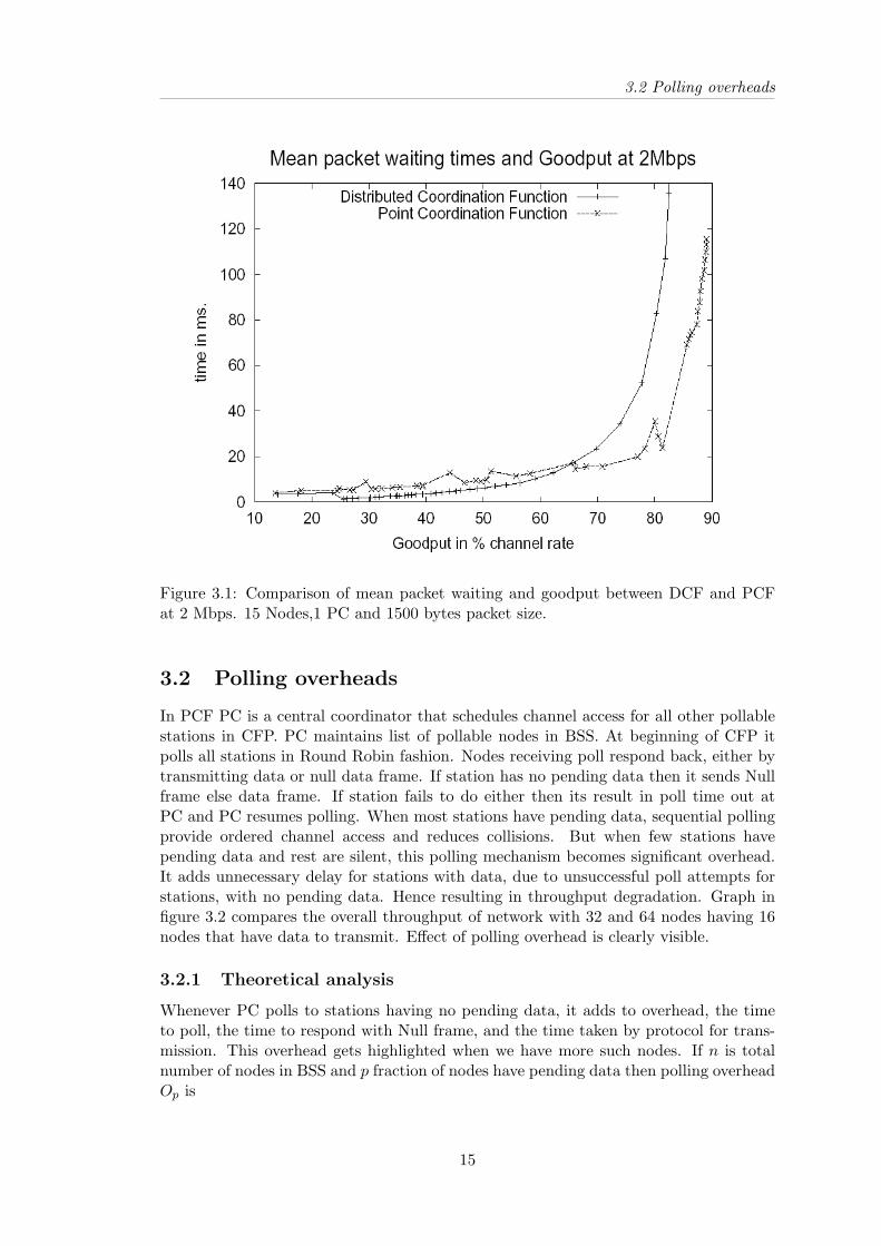
3.1 Comparison of mean packet waiting and goodput between DCF and PCFat 2 Mbps. 15 Nodes,1 PC and 1500 bytes packet size. . . . . . . . . . 15
3.2 Effect of polling overhead on network throughput . . . . . . . . . . . . . 163.3 A Transmission pattern and ring updation . . . . . . . . . . . . . . . . 203.4 Central Node Scenario . . . . . . . . . . . . . . . . . . . . . . . . . . . . 21
4.1 Solution model at PC . . . . . . . . . . . . . . . . . . . . . . . . . . . . 234.2 Example of stations/nodes in Active and Passive list. The order is im-
posed by the Node list. . . . . . . . . . . . . . . . . . . . . . . . . . . . . 234.3 Transmission sequence and list updation in CFP . . . . . . . . . . . . . 244.4 Transmission sequence and list updation in CP . . . . . . . . . . . . . . 254.5 An example of exponential increase of CW . . . . . . . . . . . . . . . . . 284.6 Extending learning to DCF . . . . . . . . . . . . . . . . . . . . . . . . . 284.7 Extending learning to DCF . . . . . . . . . . . . . . . . . . . . . . . . . 294.8 CF parameter set in beacon frame . . . . . . . . . . . . . . . . . . . . . 31
5.1 Throughput Comparison between PCF with PRRS and non optimizedPCF with RRS. Total node =32 and 25% active node . . . . . . . . . . 34
5.2 Throughput Comparison between PCF with PRRS and non optimizedPCF with RRS. Total node =64 and 25% active node . . . . . . . . . . 34
5.3 Throughput comparison of PRRS against non optimized PCF with 32nodes . . . . . . . . . . . . . . . . . . . . . . . . . . . . . . . . . . . . . 35
5.4 Throughput comparison of PRRS against non optimized PCF with 64nodes . . . . . . . . . . . . . . . . . . . . . . . . . . . . . . . . . . . . . 35
5.5 Average Delay comparison between PCF with PRRS and PCF with RRS.Total node =32 and 25% active node . . . . . . . . . . . . . . . . . . . . 36
5.6 Delay Graphs with 32 nodes and among them 50%, 75%, and 100% active. 375.7 Delay Graphs with 64 nodes and among them 25% and 50% active . . 375.8 Throughput comparison of DSP with PCF and DCF . . . . . . . . . . . 385.9 Delay comparison of DSP with PCF and DCF . . . . . . . . . . . . . . 39
vi
6.1 Throughput in PCF with PRRS for different CFP repetition interval with32 active nodes . . . . . . . . . . . . . . . . . . . . . . . . . . . . . . . . 41
6.2 Throughput in PCF with PRRS for different CFP repetition interval with8,16 and 64 active nodes. . . . . . . . . . . . . . . . . . . . . . . . . . . 41
6.3 Mean packet delays in PCF with PRRS for different CFP repetition in-terval with 8,16 and 64 active nodes. . . . . . . . . . . . . . . . . . . . . 42
6.4 Throughput comparison of PCF with PRRS for different CFP repetitioninterval with CFP adaption enabled PCF with PRRS . . . . . . . . . . 44
6.5 Delay characteristic of PCF with PRRS for different CFP repetition in-terval with CFP adaption enabled PCF with PRRS . . . . . . . . . . . 44
6.6 Throughput comparison of PCF with PRRS for different CFP repetitioninterval with CFP adaption enabled PCF with PRRS, having 8 and 16active nodes. . . . . . . . . . . . . . . . . . . . . . . . . . . . . . . . . . 45
6.7 Delay characteristic of PCF with PRRS for different CFP repetition in-terval with CFP adaption enabled PCF with PRRS, having 8 and 16active nodes. . . . . . . . . . . . . . . . . . . . . . . . . . . . . . . . . . 45
vii

Chapter 1
Introduction: Wireless LANs
1.1 Motivation
Wireless computing is a rapidly emerging technology providing users with network con-nectivity without being tethered off of a wired network. Wireless local area networks(WLANs), like their wired counterparts, are being developed to provide high bandwidthto users in a limited geographical area. WLANs are being studied as an alternative tothe high installation and maintenance costs incurred by traditional additions, deletions,and changes experienced in wired LAN infrastructures. Physical and environmentalnecessity is another driving factor in favor of WLANs.
The operational environment may not accommodate a wired network, or the networkmay be temporary and operational for a very short time, making the installation of awired network impractical. Examples where this is true include ad hoc networking needssuch as conference registration centers, campus classrooms, emergency relief centers,and tactical military environments. However, to meet these objectives, the wirelesscommunity faces certain challenges and constraints that are not imposed on their wiredcounterparts.
1.1.1 Why IEEE 802.11 WLAN
IEEE 802.11 standard is one of the prominent wireless local area network standardsbeing adopted as a mature technology. The success of the IEEE 802.11 standard hasresulted in the easy availability of commercial hardware and a proliferation of wirelessnetwork deployment, in wireless LANs as well as in mobile ad hoc networks. AlthoughIEEE 802.11 is not designed for multihop ad hoc networks, the easy availability hasmade it, most chosen MAC.
1.2 Need for Specialized Wireless MAC
Existing MAC schemes from wired networks like, CSMA/CD are not directly applicableto wireless medium. In CSMA/CD sender senses the medium to see if it is free. Ifmedium is busy, the sender waits until it is free. If the medium is free, sender startstransmitting data and also continues to listen into the medium. It stops transmissionas soon as it detects collision and sends a jam signal. In wired medium, this worksbecause more or less the same signal strength can be assumed all over the wire. Ifcollision occurs somewhere in the wire, everybody will notice it. This assumption gets
1
1.2 Need for Specialized Wireless MAC
invalidated in wireless medium, as the signal strength decreases proportionally to thesquare of distance to the sender.
In wireless medium, sender may apply carrier sense and detect an idle medium. Thus,the sender starts sending, but a collision happens at the receiver due to a second sender.Second sender may or may not be audible to first sender. Hence the sender detects nocollision, assumes that data has been transmitted without errors, but actually a collisionmight have destroyed the data at the receiver.
Besides that, wireless devices are half duplex and battery operated. They are unableto listen to the channel for collision while transmitting data.
1.2.1 Hidden and Exposed Node Problem
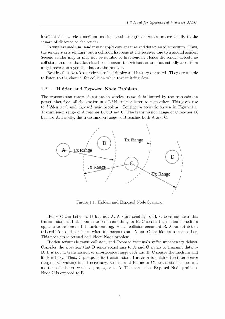
The transmission range of stations in wireless network is limited by the transmissionpower, therefore, all the station in a LAN can not listen to each other. This gives riseto hidden node and exposed node problem. Consider a scenario shown in Figure 1.1.Transmission range of A reaches B, but not C. The transmission range of C reaches B,but not A. Finally, the transmission range of B reaches both A and C.
Figure 1.1: Hidden and Exposed Node Scenario
Hence C can listen to B but not A. A start sending to B, C does not hear thistransmission, and also wants to send something to B. C senses the medium, mediumappears to be free and it starts sending. Hence collision occurs at B. A cannot detectthis collision and continues with its transmission. A and C are hidden to each other.This problem is termed as Hidden Node problem.
Hidden terminals cause collision, and Exposed terminals suffer unnecessary delays.Consider the situation that B sends something to A and C wants to transmit data toD. D is not in transmission or interference range of A and B. C senses the medium andfinds it busy. Thus, C postpone its transmission. But as A is outside the interferencerange of C, waiting is not necessary. Collision at B due to C’s transmission does notmatter as it is too weak to propagate to A. This termed as Exposed Node problem.Node C is exposed to B.
2

1.3 Challenges in Wireless LANs
1.3 Challenges in Wireless LANs
Many different and sometimes competing design goals have to be taken into account forWLANs to ensure their commercial success.
• Global operation: WLAN products should sell in all countries, therefore, manynational and international frequency regulations have to be considered.
• Low Power: Devices communicating via a WLAN are typically also wirelessdevices running on battery power. Hence, WLAN must implement special powersaving modes and power management functions.
• License-free operation: LAN operators do not want to apply for a special licensein order to be able to use the product. Thus, the equipment must operate in alicense-free band, such as the 2.4 GHz ISM band.
• Bandwidth: Bandwidth is the one of the most scarce resource in wireless net-works. The available bandwidth in wireless networks is far less than the wiredlinks.
• Link Errors: Channel fading and interference cause link errors and these errorsmay sometimes be very severe.
• Robust transmission technology: Compared to wired counterparts, WLANsoperate under difficult conditions. If they use radio transmission, many otherelectrical devices may interfere.
• Simplified spontaneous co-operation: To be useful in practice, WLANs shouldnot require complicated setup routines but should operate spontaneously afterpower up. Otherwise these LANs would not be useful for supporting e.g., ad hocmeetings, etc.
• Easy to use: LANs should not require complex management but rather work ona plug-and-play basis.
• Protection of investment: A lot of money has already been invested into wiredLANs. Hence new WLANs must protect this investment by being inter operablewith the existing networks.
• Safety and security: Most important concern is of safety and security. WLANsshould be safe to operate, especially regarding low radiation. Furthermore, nousers should be able to read personal data during transmission i.e., encryptionmechanism should be integrated. The network should also take into account userprivacy.
• Transparency for application: Existing applications should continue to runover WLANs. The fact of wireless access and mobility should be hidden if notrelevant.
1.4 IEEE 802.11 standard
IEEE 802.11 MAC features two mode of operations: Distributed Coordinating Function(DCF) and Point Coordinating Function (PCF). DCF is CSMA/CA based random
3

1.5 Problem Statement
access protocol that uses random backoff to avoid collision. It uses RTS/CTS exchangemechanism to reserve channel when packet size is above the RTSthreshold. It reducesthe hidden terminal effect (section 1.2.1). PCF provide centralized scheduled access tochannel. It comprises of chain of contention free period (CFP) and contention period(CP). DCF rules are followed in the CP. In the CFP point coordinator (PC) polls thenode one by one and grant access to channel. New stations that need to get enrolled inpoll list, send request in CP.
1.5 Problem Statement
Our work aims at optimizing overall performance of IEEE 802.11 MAC. Although wehave tried to keep solution robust enough to suit different traffic scenarios, our mainfocus is on traffic directed towards a central node. Both DCF and PCF do not performwell under all load regime. Each has its own pros and cons depending upon differentload condition. When only small number of nodes have data to transmit PCF incurspolling overheads, and at high load DCF performance degrades. We think there is needto dynamically adapt IEEE 802.11 MAC under varying load, such that coexistence ofboth the modes can be exploited.
Besides that, performance of DCF and PCF depends highly upon their various con-figuration parameters. Studies shows that good values of these configuration parametersdepend upon network load. Statically configured values result in degraded throughputunder varying load. So there is need to dynamically adapt these values.
We have proposed learning based protocol to reduce polling overheads in PCF andto dynamically adapt configuration parameters. To exploit better half of both PCF andDCF, we have proposed a protocol to dynamically switch between two modes.
1.6 Thesis outline
In this thesis, in next chapter we start with summarization of existing IEEE 802.11bWLAN standard. We emphasize fully on the MAC sub-layer explaining both DCFand PCF. Chapter 3 discuss in depth view of problems, we attacking and also presenttheoretical analysis of problem. Moving further, various existing approaches to dealwith performance issue are then discussed, along with arguments for the need of ourapproach.
Following the track, Chapter 4 explains our solutions to problem, termed as PriorityRound Robin Scheduling (PRRS) and Dynamic Switching Protocol (DSP). Chapter 5describes simulation scenario and performance metric used by us. Following this, weanalyze our results that lead to further optimization of our solution, PRRS in Chapter6. Chapter 7 then concludes our work and points to future work to be explored.
4

Chapter 2
MAC Sublayer in IEEE 802.11
The IEEE standard 802.11 specifies the most famous family of WLANs in which manyproducts are already available. Standard belongs to the group of 802.x LAN standards,e.g., 802.3 Ethernet or 802.5 Token Ring. This means that the standard specifies thephysical and medium access layer adapted to the special requirements of wireless LANs,but offers the same interface as the others to higher layers to maintain interoperability.
2.1 Scope and Purpose of IEEE 802.11 standard
The scope of this standard is to develop a medium access control (MAC) and physi-cal layer (PHY) specification for wireless connectivity for fixed, portable, and movingstations within a local area.
The purpose of this standard is to provide wireless connectivity to automatic ma-chinery, equipment, or stations that require rapid deployment, which may be portableor hand-held, or which may be mounted on moving vehicles within a local area. Thisstandard also offers regulatory bodies a means of standardizing access to one or morefrequency bands for the purpose of local area communication.
Primary goal of the standard was the specification of a simple and robust WLANwhich offers time-bounded and asynchronous services. Furthermore, the MAC layershould be able to operate with the multiple physical layers, each of which exhibits adifferent medium sense and transmission characteristic. Candidates for physical layerswere infrared and spread spectrum radio transmission techniques.
Additionally features of the WLAN should include the support of the power man-agement, the handling of hidden nodes, and the ability to operate worldwide.
2.2 System Architecture
The basic service set (BSS) is the fundamental building block of the IEEE 802.11 ar-chitecture. A BSS is defined as a group of stations that are under the direct controlof a single coordination function (i.e., a DCF or PCF) which is defined below. Thegeographical area covered by the BSS is known as the basic service area (BSA), whichis analogous to a cell in a cellular communications network. Conceptually, all stationsin a BSS can communicate directly with all other stations in a BSS. However, transmis-sion medium degradations due to multipath fading, or interference from nearby BSSsreusing the same physical-layer characteristics (e.g., frequency and spreading code, orhopping pattern), can cause some stations to appear hidden from other stations. An
5

2.2 System Architecture
ad hoc network is a deliberate grouping of stations into a single BSS for the purposesof internetworked communications without the aid of an infrastructure network. Figure2.1 is an illustration of an independent BSS (IBSS), which is the formal name of an adhoc network in the IEEE 802.11 standard. Any station can establish a direct communi-cations session with any other station in the BSS, without the requirement of channelingall traffic through a centralized access point (AP).
Figure 2.1: Sketch of an ad hoc network
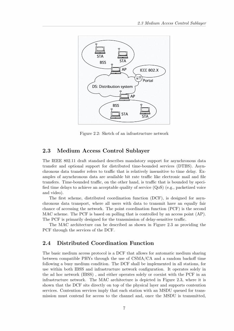
In contrast to the ad hoc network, infrastructure networks are established to providewireless users with specific services and range extension. Infrastructure networks in thecontext of IEEE 802.11 are established using APs. The AP is analogous to the basestation in a cellular communications network. The AP supports range extension byproviding the integration points necessary for network connectivity between multipleBSSs, thus forming an extended service set (ESS). The ESS has the appearance ofone large BSS to the logical link control (LLC) sublayer of each station (STA). TheESS consists of multiple BSSs that are integrated together using a common distributionsystem (DS). The DS can be thought of as a backbone network that is responsiblefor MAC-level transport of MAC service data units (MSDUs). The DS, as specifiedby IEEE 802.11, is implementation independent. Therefore, the DS could be a wiredIEEE 802.3 Ethernet LAN, IEEE 802.4 token bus LAN, IEEE 802.5 token ring LAN,fiber distributed data interface (FDDI) metropolitan area network (MAN), or anotherIEEE 802.11 wireless medium. Note that while the DS could physically be the sametransmission medium as the BSS, they are logically different, because the DS is solelyused as a transport backbone to transfer packets between different BSSs in the ESS. AnESS can also provide gateway access for wireless users into a wired network such as theInternet. This is accomplished via a device known as a portal. The portal is a logicalentity that specifies the integration point on the DS where the IEEE 802.11 networkintegrates with a non-IEEE 802.11 network. If the network is an IEEE 802.X, theportal incorporates functions which are analogous to a bridge; that is, it provides rangeextension and the translation between different frame formats. Figure 2.2 illustrates asimple ESS developed with two BSSs, a DS, and a portal access to a wired LAN.
6
2.3 Medium Access Control Sublayer
Figure 2.2: Sketch of an infrastructure network
2.3 Medium Access Control Sublayer
The IEEE 802.11 draft standard describes mandatory support for asynchronous datatransfer and optional support for distributed time-bounded services (DTBS). Asyn-chronous data transfer refers to traffic that is relatively insensitive to time delay. Ex-amples of asynchronous data are available bit rate traffic like electronic mail and filetransfers. Time-bounded traffic, on the other hand, is traffic that is bounded by speci-fied time delays to achieve an acceptable quality of service (QoS) (e.g., packetized voiceand video).
The first scheme, distributed coordination function (DCF), is designed for asyn-chronous data transport, where all users with data to transmit have an equally fairchance of accessing the network. The point coordination function (PCF) is the secondMAC scheme. The PCF is based on polling that is controlled by an access point (AP).The PCF is primarily designed for the transmission of delay-sensitive traffic.
The MAC architecture can be described as shown in Figure 2.3 as providing thePCF through the services of the DCF.
2.4 Distributed Coordination Function
The basic medium access protocol is a DCF that allows for automatic medium sharingbetween compatible PHYs through the use of CSMA/CA and a random backoff timefollowing a busy medium condition. The DCF shall be implemented in all stations, foruse within both IBSS and infrastructure network configuration. It operates solely inthe ad hoc network (IBSS) , and either operates solely or coexist with the PCF in aninfrastructure network. The MAC architecture is depicted in Figure 2.3, where it isshown that the DCF sits directly on top of the physical layer and supports contentionservices. Contention services imply that each station with an MSDU queued for trans-mission must contend for access to the channel and, once the MSDU is transmitted,
7

2.4 Distributed Coordination Function
Figure 2.3: MAC Architecture
must recontend for access to the channel for all subsequent frames. Contention servicespromote fair access to the channel for all stations.
The CSMA/CA protocol is designed to reduce the collision probability betweenmultiple stations accessing a medium, at the point where collisions would most likelyoccur. Just after the medium becomes idle following a busy medium, is when thehighest probability of a collision exists. This is because multiple stations could havebeen waiting for the medium to become available again. This is the situation thatnecessitates a random backoff procedure to resolve medium contention conflicts.
Station that needs to transmit data, first sense the carrier. In IEEE 802.11, carriersensing is performed at both the air interface, referred to as physical carrier sensing,and at the MAC sublayer, referred to as virtual carrier sensing. Physical carrier sensingdetects the presence of other IEEE 802.11 WLAN users by analyzing all detected packets,and also detects activity in the channel via relative signal strength from other sources.
A virtual carrier-sense mechanism shall be provided by the MAC. This mechanismis referred to as the network allocation vector (NAV). The NAV maintains a predictionof future traffic on the medium based on duration information that is announced inRTS/CTS frames prior to the actual exchange of data. The duration information is alsoavailable in the MAC headers of other frames sent during the CP. The Duration/ IDfield defines the period of time that the medium is to be reserved to transmit the actualdata frame and the returning ACK frame. Stations in the BSS use the information inthe duration field to adjust their network allocation vector (NAV), which indicates theamount of time that must elapse until the current transmission session is complete andthe channel can be sampled again for idle status. The channel is marked busy if eitherthe physical or virtual carrier sensing mechanisms indicate the channel is busy.
Priority access to the wireless medium is controlled through the use of interframespace (IFS) time intervals between the transmission of frames. The IFS intervals aremandatory periods of idle time on the transmission medium. Three IFS intervals arespecified in the standard: short IFS (SIFS), point coordination function IFS (PIFS),and DCF-IFS (DIFS). The SIFS interval is the smallest IFS, followed by PIFS andDIFS, respectively. Stations only required to wait a SIFS have priority access over thosestations required to wait a PIFS or DIFS before transmitting; therefore, SIFS has thehighest-priority access to the communications medium. For the basic access method,when a station senses the channel is idle, the station waits for a DIFS period and samples
8

2.4 Distributed Coordination Function
the channel again. If the channel is still idle, the station transmits an MPDU. The re-ceiving station calculates the checksum and determines whether the packet was receivedcorrectly. Upon receipt of a correct packet, the receiving station waits a SIFS intervaland transmits a positive acknowledgment frame (ACK) back to the source station, indi-cating that the transmission was successful. Figure 2.4 is a timing diagram illustratingthe successful transmission of a data frame. When the data frame is transmitted, theduration field of the frame is used to let all stations in the BSS know how long themedium will be busy. All stations hearing the data frame adjust their NAV based onthe duration field value, which includes the SIFS interval and the ACK following thedata frame.
Figure 2.4: Transmission of an MPDU without RTS/CTS
Since a source station in a BSS cannot hear its own transmissions, when a collisionoccurs, the source continues transmitting the complete MPDU. If the MPDU is large(e.g., 2300 bytes), a lot of channel bandwidth is wasted due to a corrupt MPDU. RTSand CTS control frames can be used by a station to reserve channel bandwidth prior tothe transmission of an MPDU and to minimize the amount of bandwidth wasted whencollisions occur. RTS and CTS control frames are relatively small (RTS is 20 bytes andCTS is 14 bytes) when compared to the maximum data frame size (2346 bytes). The RTScontrol frame is first transmitted by the source station (after successfully contending forthe channel) with a data or management frame queued for transmission to a specifieddestination station. All stations in the BSS, hearing the RTS packet, read the durationfield and set their NAVs accordingly. The destination station responds to the RTSpacket with a CTS packet after an SIFS idle period has elapsed. Stations hearing theCTS packet look at the duration field and again update their NAV. Upon successfulreception of the CTS, the source station is virtually assured that the medium is stableand reserved for successful transmission of the MPDU. Note that stations are capableof updating their NAVs based on the RTS from the source station and CTS from thedestination station, which helps to combat the hidden terminal problem [1.2.1]. Figure2.5 illustrates the transmission of an MPDU using the RTS/CTS mechanism. Stationscan choose to never use RTS/CTS, use RTS/CTS whenever the MSDU exceeds thevalue of RTS Threshold (manageable parameter), or always use RTS/CTS. If a collision
9

2.4 Distributed Coordination Function
occurs with an RTS or CTS MPDU, far less bandwidth is wasted when compared to alarge data MPDU. However, for a lightly loaded medium, additional delay is imposedby the overhead of the RTS/CTS frames.
Figure 2.5: Transmission of an MPDU using RTS/CTS
Large MSDUs handed down from the LLC to the MAC may require fragmenta-tion to increase transmission reliability. To determine whether to perform fragmenta-tion, MPDUs are compared to the manageable parameter Fragmentation Threshold. Ifthe MPDU size exceeds the value of Fragmentation Threshold, the MSDU is brokeninto multiple fragments. The resulting MPDUs are of size Fragmentation Threshold,with exception of the last MPDU, which is of variable size not to exceed Fragmenta-tion Threshold. When an MSDU is fragmented, all fragments are transmitted sequen-tially. The channel is not released until the complete MSDU has been transmittedsuccessfully, or the source station fails to receive an acknowledgment for a transmittedfragment. The destination station positively acknowledges each successfully receivedfragment by sending a DCF ACK back to the source station. The source station main-tains control of the channel throughout the transmission of the MSDU by waiting onlyan SIFS period after receiving an ACK and transmitting the next fragment. When anACK is not received for a previously transmitted frame, the source station halts trans-mission and recontends for the channel. Upon gaining access to the channel, the sourcestarts transmitting with the last unacknowledged fragment.
If RTS and CTS are used, only the first fragment is sent using the handshakingmechanism. The duration value of RTS and CTS only accounts for the transmissionof the first fragment through the receipt of its ACK. Stations in the BSS thereaftermaintain their NAV by extracting the duration information from all subsequent frag-ments. The collision avoidance portion of CSMA/CA is performed through a randombackoff procedure. If a station with a frame to transmit initially senses the channel tobe busy; then the station waits until the channel becomes idle for a DIFS period, andthen computes a random backoff time. For IEEE 802.11, time is slotted in time periodsthat correspond to a Slot Time. Unlike slotted Aloha, where the slot time is equal tothe transmission time of one packet, the Slot Time used in IEEE 802.11 is much smallerthan an MPDU and is used to define the IFS intervals and determine the backoff time
10

2.5 Point Coordination Function
for stations in the CP. The Slot Time is different for each physical layer implementa-tion. The random backoff time is an integer value that corresponds to a number of timeslots. Initially, the station computes a backoff time in the range equals size of contentionwindow (CW). After the medium becomes idle after a DIFS period, stations decrementtheir backoff timer until the medium becomes busy again or the timer reaches zero. Ifthe timer has not reached zero and the medium becomes busy, the station freezes itstimer. When the timer is finally decremented to zero, the station transmits its frame. Iftwo or more stations decrement to zero at the same time, a collision will occur, and eachstation will have to generate a new backoff time but for each retransmission attempt,station doubles its contention window. The advantage of this channel access methodis that it promotes fairness among stations, but its weakness is that it probably couldnot support DTBS. Fairness is maintained because each station must recontend for thechannel after every transmission of an MSDU. All stations have equal probability ofgaining access to the channel after each DIFS interval. Time-bounded services typicallysupport applications such as packetized voice or video that must be maintained witha specified minimum delay. With DCF, there is no mechanism to guarantee minimumdelay to stations supporting time-bounded services.
2.5 Point Coordination Function
The PCF provides contention-free frame transfer. The PC shall reside in the AP. It is anoption for an AP to be able to become the PC. All stations inherently obey the mediumaccess rules of the PCF, because these rules are based on the DCF, and they set theirNAV at the beginning of each CFP. The operating characteristics of the PCF are suchthat all stations are able to operate properly in the presence of a BSS in which a PC isoperating, and, if associated with a point-coordinated BSS, are able to receive all framessent under PCF control. It is also an option for a station to be able to respond to acontention-free poll (CF-Poll) received from a PC. A station that is able to respond toCF-Polls is referred to as being CF-Pollable, and may request to be polled by an activePC. CF-Pollable stations and the PC do not use RTS/CTS in the CFP. When polledby the PC, a CFPollable station may transmit only one MPDU, which can be to anydestination (not just to the PC), and may piggyback the acknowledgment of a framereceived from the PC using particular data frame subtypes for this transmission. If thedata frame is not in turn acknowledged, the CF-Pollable station shall not retransmit theframe unless it is polled again by the PC, or it decides to retransmit during the CP. If theaddressed recipient of a CF transmission is not CF-Pollable, that station acknowledgesthe transmission using the DCF acknowledgment rules, and the PC retains control ofthe medium. A PC may use contention-free frame transfer solely for delivery of framesto stations, and never to poll non-CF-Pollable stations.
The PCF controls frame transfers during a CFP. The CFP shall alternate with a CP,when the DCF controls frame transfers, as shown in Figure 2.6.Combined CFP and CPis termed as one superframe. Each CFP shall begin with a Beacon frame that containsa DTIM element (hereafter referred to as a DTIM ). The CFPs shall occur at a definedrepetition rate, which shall be synchronized with the beacon interval as specified in thefollowing paragraphs.
The PC generates CFPs at the contention-free repetition rate (CFPRate), which isdefined as a number of DTIM intervals. The PC shall determine the CFPRate to usefrom the CFPRate parameter in the CF Parameter Set. This value, in units of DTIMintervals, shall be communicated to other stations in the BSS in the CFPPeriod field of
11

2.5 Point Coordination Function
the CF Parameter Set element of Beacon frames.
Figure 2.6: Superframe CFP/CP alternation
The length of the CFP is controlled by the PC, with maximum duration specified bythe value of the CFPMaxDuration Parameter in the CF Parameter Set at the PC. ThePC may terminate any CFP at or before the aCFPMaxDuration, based on availabletraffic and size of the polling list.
The contention-free transfer protocol is based on a polling scheme controlled by a PCoperating at the AP of the BSS. The PC gains control of the medium at the beginning ofthe CFP and attempts to maintain control for the entire CFP by waiting a shorter timebetween transmissions than the stations using the DCF access procedure. All stationsin the BSS (other than the PC) set their NAVs to the CFPMaxDuration value at thenominal start time of each CFP. This prevents most contention by preventing non-polledtransmissions by stations whether or not they are CF-Pollable.The PC shall transmit aCF-End or CF-End+ACK frame at the end of each CFP. A station that receives eitherof these frames, from any BSS, shall reset its NAV.
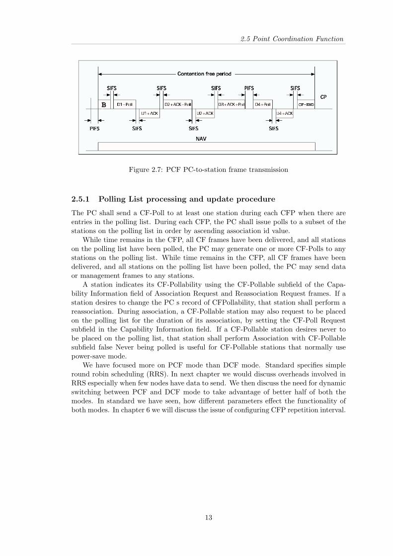
At the nominal start of the CFP, the PC senses the medium. If the medium remainsidle for a PIFS interval, the PC transmits a beacon frame to initiate the CFP. The PCstarts CF transmission a SIFS interval after the beacon frame is transmitted by sendinga CF-Poll (no data), Data, or Data+CF-Poll frame. The PC can immediately terminatethe CFP by transmitting a CF-End frame, which is common if the network is lightlyloaded and the PC has no traffic buffered. If a CF-aware station receives a CF-Poll (nodata) frame from the PC, the station can respond to the PC after a SIFS idle period,with a CF-ACK (no data) or a Data + CF-ACK frame. If the PC receives a Data +CFAck frame from a station, the PC can send a Data + CFACK + CF-Poll frame to adifferent station, where the CF-ACK portion of the frame is used to acknowledge receiptof the previous data frame. The ability to combine polling and acknowledgment frameswith data frames, transmitted between stations and the PC, was designed to improveefficiency. If the PC transmits a CF-Poll (no data) frame and the destination stationdoes not have a data frame to transmit, the station sends a Null Function (no data)frame back to the PC. Figure 2.7 illustrates the transmission of frames between the PCand a station, and vice versa. If the PC fails to receive an ACK for a transmitted dataframe, the PC waits a PIFS interval and continues transmitting to the next station in thepolling list. After receiving the poll from the PC, as described above, the station maychoose to transmit a frame to another station in the BSS. When the destination stationreceives the frame, a DCF ACK is returned to the source station, and the PC waits aPIFS interval following the ACK frame before transmitting any additional frames.
12
2.5 Point Coordination Function
Figure 2.7: PCF PC-to-station frame transmission
2.5.1 Polling List processing and update procedure
The PC shall send a CF-Poll to at least one station during each CFP when there areentries in the polling list. During each CFP, the PC shall issue polls to a subset of thestations on the polling list in order by ascending association id value.
While time remains in the CFP, all CF frames have been delivered, and all stationson the polling list have been polled, the PC may generate one or more CF-Polls to anystations on the polling list. While time remains in the CFP, all CF frames have beendelivered, and all stations on the polling list have been polled, the PC may send dataor management frames to any stations.
A station indicates its CF-Pollability using the CF-Pollable subfield of the Capa-bility Information field of Association Request and Reassociation Request frames. If astation desires to change the PC s record of CFPollability, that station shall perform areassociation. During association, a CF-Pollable station may also request to be placedon the polling list for the duration of its association, by setting the CF-Poll Requestsubfield in the Capability Information field. If a CF-Pollable station desires never tobe placed on the polling list, that station shall perform Association with CF-Pollablesubfield false Never being polled is useful for CF-Pollable stations that normally usepower-save mode.
We have focused more on PCF mode than DCF mode. Standard specifies simpleround robin scheduling (RRS). In next chapter we would discuss overheads involved inRRS especially when few nodes have data to send. We then discuss the need for dynamicswitching between PCF and DCF mode to take advantage of better half of both themodes. In standard we have seen, how different parameters effect the functionality ofboth modes. In chapter 6 we will discuss the issue of configuring CFP repetition interval.
13

Chapter 3
Problem Analysis and RelatedWork
In this work we have focused on three problem areas that lead to performance degrada-tion in IEEE 802.11 WLAN. One major problem with PCF that gets highlighted whensmall fraction of associated and pollable nodes in BSS are sending data, and rest aresilent. This results in significant polling overheads that wastes the scare channel band-width. Second problem area is to define protocol for dynamic switching between twomodes. Mean packet delays can be reduced by having DCF when less nodes have pend-ing data and PCF otherwise. Third problem area is statically configured configurationparameters of PCF and DCF. Depending on the network configuration, the standardcan operate far from the theoretical throughput limits.
3.1 Need for Switching between PCF and DCF
The DCF mode of IEEE 802.11 exerts a CSMA/CA approach, which is in fact a 1-persistent random access protocol with delay. Random access protocol works satisfac-torily as long as network size is limited. Here by network size we mean number of nodethat have pending data in BSS, i.e. in transmission range of central node. Load isdefined as total bits transmitted by all stations in BSS per second. As network expands,competition for accessing shared wireless channel increases. This results in throughputdegradation and more delay because of more collision and increased time spent for ne-gotiating channel access. We need ordered way to schedule the channel access at highloads.
IEEE 802.11 provide another more organized way to grant channel access calledPCF. But better management always poses some overheads that become prominentunder low load scenarios. Similar story appears here. DCF whose performance degradesat high load and in big size network, provide lesser delays at low load. On counter side,scheduled MAC like PCF with centralized control better utilize resources at high loadand in large network. But when few nodes have data to send PCF perform worse thanDCF because of scheduling overhead in PCF (section 3.2). Graph ∗ shown in figure 3.1presents goodput and delay at different load. PCF starts with slightly high delay, butit remains low and constant up to 80% goodput. In DCF beyond 60% load the delayincreases exponentially. We think dynamic switching between them will increase thechannel capacity and offer lower delays.
∗Graph by Wolisz, et. al [6]
14
3.2 Polling overheads
Figure 3.1: Comparison of mean packet waiting and goodput between DCF and PCFat 2 Mbps. 15 Nodes,1 PC and 1500 bytes packet size.
3.2 Polling overheads
In PCF PC is a central coordinator that schedules channel access for all other pollablestations in CFP. PC maintains list of pollable nodes in BSS. At beginning of CFP itpolls all stations in Round Robin fashion. Nodes receiving poll respond back, either bytransmitting data or null data frame. If station has no pending data then it sends Nullframe else data frame. If station fails to do either then its result in poll time out atPC and PC resumes polling. When most stations have pending data, sequential pollingprovide ordered channel access and reduces collisions. But when few stations havepending data and rest are silent, this polling mechanism becomes significant overhead.It adds unnecessary delay for stations with data, due to unsuccessful poll attempts forstations, with no pending data. Hence resulting in throughput degradation. Graph infigure 3.2 compares the overall throughput of network with 32 and 64 nodes having 16nodes that have data to transmit. Effect of polling overhead is clearly visible.
3.2.1 Theoretical analysis
Whenever PC polls to stations having no pending data, it adds to overhead, the timeto poll, the time to respond with Null frame, and the time taken by protocol for trans-mission. This overhead gets highlighted when we have more such nodes. If n is totalnumber of nodes in BSS and p fraction of nodes have pending data then polling overheadOp is
15

3.2 Polling overheads
Figure 3.2: Effect of polling overhead on network throughput
Parameter Symbol ValueSIFS Interval SIFS 10µs
Channel B/w bw 2MbpsCF-Poll size SizePoll 20 bytes
Ack Size SizeAck 14 bytesNull Frame Size SizeNull 34 bytes
Time to send poll TPoll SizePoll × 8/bw
Time to send Null Frame TNull SizeNull × 8/bw
Time to send Data TData Psize × 8/bw
Time to send Ack TAck SizeAck × 8/bw
Table 3.1: 802.11b Default parameters
Op = p ∗ n ∗ TPollFail
where TPollFail is worst case time ∗ overhead due to unsuccessful poll attempt given as
TPollFail = TPoll + SIFS + TNull + SIFS
where TPoll and TNull is time to send poll and send Null data frame respectively. Ifwe assume mean packet size be Psize then time for successful poll attempt is given byTPollSuccess.
TPollSuccess = TPoll + SIFS + TData + SIFS + TAck + SIFS
Now we can compute percentage overhead as ratio of TPollFail and CFP duration.Default values for IEEE 802.11b parameters are depicted in table 3.1. Polling overheadis presented as percentage of CFP get wasted in unsuccessful polling attempts. Assumesingle complete round of polling. Table 3.2 shows polling overheads in different scenarios
∗Frame type CFPoll+DATA+ACK can reduce this
16

3.3 Need for Dynamic Tuning Configuration parameter
using different values of p and Psize. Regime where performance can be improved byreducing polling overhead is quite clear. As mean packet size reduces and number ofnodes sending null frame increases, the effect of overhead heightens. With increase intotal number of nodes in BSS, overall throughput degradation will also increase.
Percentage of active Nodes
Packet sizein bytes
12.5% 25% 50% 75%300 52.37% 32.03% 13.57% 4.97%500 41.77% 23.51% 9.29% 3.29%1000 27.74% 13.97% 5.19% 1.78%1500 20.76% 10.09% 3.60% 1.22%
Table 3.2: Percentage polling overheads with active nodes percentage 10,25, 50, and 75and packet size (bytes) 300,500,100,and 1500
3.3 Need for Dynamic Tuning Configuration parameter
Both DCF and PCF has lot of configuration parameters that directly affects their func-tioning. Good values of these parameter is highly dependent on network size and trafficload. Besides network load, traffic model and mobility pattern also play significant rolein deciding its performance, as these factors too affect configuration parameters. Table3.3 list some main parameters that need to accurately configured.
It is not always possible to accurately approximate the network size and load andthen statically configured various configuration parameters. Even if network adminis-trator has certain approximation, even then its true that the approximation doesn’t holdaround the clock. So we though that there is a need to have some intelligent systemthat learns network continuously and dynamically reconfigures the parameters.
Parameter Meaning EffectRTS threshold MPDU size above
which RTS/CTS isused
Directly monitor effect of hidden nodes. Valuedepend upon number of competing stations
CW min Minimum number ofbackoff slots
Directly control number of collision, Value de-pend upon number of competing stations
aFragmentationThreshold
Size above whichMPDU need to befragmented
Decides probability of successful transmission
CFP repetitioninterval
Decides CFP and CPduration
Depend on number of nodes to service anddirectly affect delays
Table 3.3: Configuration parameters
17

3.4 Tuning of DCF
3.4 Tuning of DCF
DCF mode of operation has been studied more than PCF. Frederico, et. al [12] concludedthat appropriate tuning of the backoff algorithm can drive the DCF mode operationclose to the theoretical throughput limit. They adopted p-persistent backoff algorithmto show that it is possible, by observing the network status, to estimate the averagebackoff window size that maximizes the throughput.
Wolisz,et. [20, 21] al have identified the backoff strategy and RTS/CTS messageexchange as the elements with crucial impact on the network performance. They showedvia simulation that it is reasonable only to use RTS/CTS mechanism when load ishigh. They extensively studied the effect of hidden terminals (section 1.2.1) and needof RTS/CTS using different packet sizes and varying number of stations. Chayya, et.al [13] also concluded same result regarding the use of RTS/CTS mechanism. They alsostudied the effect of station location on probability of success.
3.5 Solution strategy
Our solution aims to fine tune existing IEEE 802.11 LAN such that it shows betterperformance results under all load regime. We tried to adhere to existing standardand suggest minimal changes to meet our goals. As standard allows coexistence ofboth functionality, so our effort aims to devise solution that includes better half ofboth functionalities. We have used a network monitoring layer at the PC that learnsnetwork and tries to approximate current network load. Using information generatedby monitoring layer, we have designed simple protocols. First step towards our goal isPRRS priority round robin scheduling that replaces simple round robin scheduling inPCF. Tuning further, we devise a algorithm for dynamically configuring CFP repetitioninterval. Next step is to dynamically switch between DCF and PCF mode and exploitthere coexistence power. We have provided DSP, a dynamic switching protocol to switchbetween either modes.
3.6 Related Work
To the best of our knowledge, there is very little literature , that deals with pollingoverhead in PCF. People have mentioned the problem earlier and there also exist someproposed solution to deal with it. Besides that people have depicted the importanceof polling for providing QoS service in IEEE 802.11 WLAN. New upcoming standardfor QoS, IEEE 802.11e [17] defines intelligent polling based HCF ∗ that assign timebounded transmission opportunities to all stations. Visser,et. al [19] have studied theimpact of superframe length (CFP+CP), on the voice transmission over IEEE 802.11 inPCF mode.
3.6.1 Signaling Polling Information
Wolisz, et al [6] have identified the somewhat similar problem and proposed solutionsbased on implicit and explicit signaling. According to them mobile nodes have to providethe AP with suitable polling information, to reduce polling overhead. Two methodproposed by them for signaling polling information is:
∗built on top of Enhanced DCF
18

3.6 Related Work
1. Explicit signaling: Node signal its transmission request in the contention periodof the superframe by means of a dedicated short signaling frame.
2. Implicit signaling: Node indicates by means of the recently transmitted framethat there are more packets pending.
First approach added additional overhead of signaling packet and second one requiresexisting frame structure to be modified.
3.6.2 STRP: Efficient Polling MAC
Oran sharon and Eitan Altman [15] suggest STRP, a efficient polling MAC which ex-ploits the capture phenomena and enables simultaneous polling and transmission ofinformation packet. Their proposal tries to overcome the inefficiency encountered (un-successful poll attempts) when only part of the stations have packets to transmit bytaking advantage of the capture phenomena in radio channel.
Simultaneous Transmission and Response Polling(STRP) utilizes three logical ringat the BS. First System Ring contains all the stations in the BSS, which are arranged incyclic. Other two logical rings, Active ring and Idle ring contains stations that notifiedBSS that they have packets to transmit and and those that notified BSS that they donot have packets to transmit respectively. Order of stations in logical rings is definedby system ring.
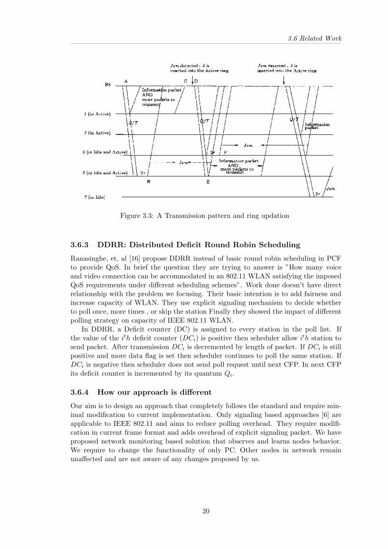
BS enables a station in the active ring to transmit data and polls a station in the idlering by the same control packet denoted by Query/Transmit (Q/T). It contains identityof the station(I) in the active ring as well as identity of station(J) in the idle ring. WhenI receive Q/T packet it begins transmission as per predefined rules. When J receivesthe same packet, it waits for predefined time units and then begins to transmit a Jamsignal by a weaker signal than I, if it has packet(s) to transmit and wants to join theactive ring. Jam from J collides with I’s transmission but since J transmits the Jam bya weaker signal, by the capture effect, BS succeeds in receiving the packet from I. I whiletransmitting packet also explicit signals the BS if it wants to stay in the active ring. If Idoes not signals BS that it wants to stay in active list, then it is shifted to idle list. Afterdetecting the end of packet from I, the BS continues to listen to the upstream link. If itdetects the Jam signal from J then J is moved to the active list. J continuously transmitthe Jam signal until it hears the next control packets from the BS. Hence signal controlpacket serve multiple purpose like, enables station in the active ring to transmit, pollsstation in the idle ring, and may also give indication to some station in the idle ring toend the jam signal. Figure 3.3 shows how the BS transmits to the stations in the logicalring.
Although approach succeeds in reducing in the polling overhead caused by stationshaving no pending data to transmit, but it adds lots of prerequisite. To implementsimilar approach in existing PCF, need to change the existing frame structure of controlpackets or to add new control packet. Most important prerequisite is that the aboveapproach requires two separate transmission links in the system, an Upstream and aDownstream, capable of working simultaneously. And of course it needs to implementcapture phenomena.
19
3.6 Related Work
Figure 3.3: A Transmission pattern and ring updation
3.6.3 DDRR: Distributed Deficit Round Robin Scheduling
Ranasinghe, et, al [16] propose DDRR instead of basic round robin scheduling in PCFto provide QoS. In brief the question they are trying to answer is ”How many voiceand video connection can be accommodated in an 802.11 WLAN satisfying the imposedQoS requirements under different scheduling schemes”. Work done doesn’t have directrelationship with the problem we focusing. Their basic intention is to add fairness andincrease capacity of WLAN. They use explicit signaling mechanism to decide whetherto poll once, more times , or skip the station Finally they showed the impact of differentpolling strategy on capacity of IEEE 802.11 WLAN.
In DDRR, a Deficit counter (DC) is assigned to every station in the poll list. Ifthe value of the ith deficit counter (DCi) is positive then scheduler allow ith station tosend packet. After transmission DCi is decremented by length of packet. If DCi is stillpositive and more data flag is set then scheduler continues to poll the same station. IfDCi is negative then scheduler does not send poll request until next CFP. In next CFPits deficit counter is incremented by its quantum Qi.
3.6.4 How our approach is different
Our aim is to design an approach that completely follows the standard and require min-imal modification to current implementation. Only signaling based approaches [6] areapplicable to IEEE 802.11 and aims to reduce polling overhead. They require modifi-cation in current frame format and adds overhead of explicit signaling packet. We haveproposed network monitoring based solution that observes and learns nodes behavior.We require to change the functionality of only PC. Other nodes in network remainunaffected and are not aware of any changes proposed by us.
20

3.7 Application in Ad hoc Networks
3.7 Application in Ad hoc Networks
Closed-User-Group Multihop Ad Hoc networks have an increasing role to play in thefuture networks. Well known examples are military networks, disaster managementnetworks, tourist information center, inquiry booth, etc. Such networks will almostcertainly have one or more command and control centers and traffic will be skewedtowards them i.e., most nodes will send traffic to the command/control center. Such atraffic pattern has not yet been studied in literature. Problems in DCF gets aggravatedin such traffic pattern.
Our focus is on such networks. Central commander node that can be a access point,is surrounded by other nodes that communicate with it. Nodes are in the range of accesspoint but they may not be in range of other nodes in network.
Figure 3.4: Central Node Scenario
21
Chapter 4
Optimizing PCF mode of IEEE802.11 MAC
4.1 Why PCF
In recent years there has been an increasing trend towards personal computers andworkstations becoming portable and mobile. People need the same service quality as inwired network. Future demands support of voice and other real time traffic. We believePCF will better satisfy the future needs. Existing studies shows the PCF ability toprovide better quality of service and support of voice and real time traffic. Upcomingstandard for QoS in IEEE 802.11 MAC, 802.11e [17] also justify our keen interest inoptimizing PCF. Malathi,et. al [18] discuss the support of voice services via PCF mode.We are not focusing on QoS issues, support of voice and real time data, etc. We haveproposed generalised improvement in PCF that we believe will enhance existing IEEE802.11 mac.
4.2 Solution Overview
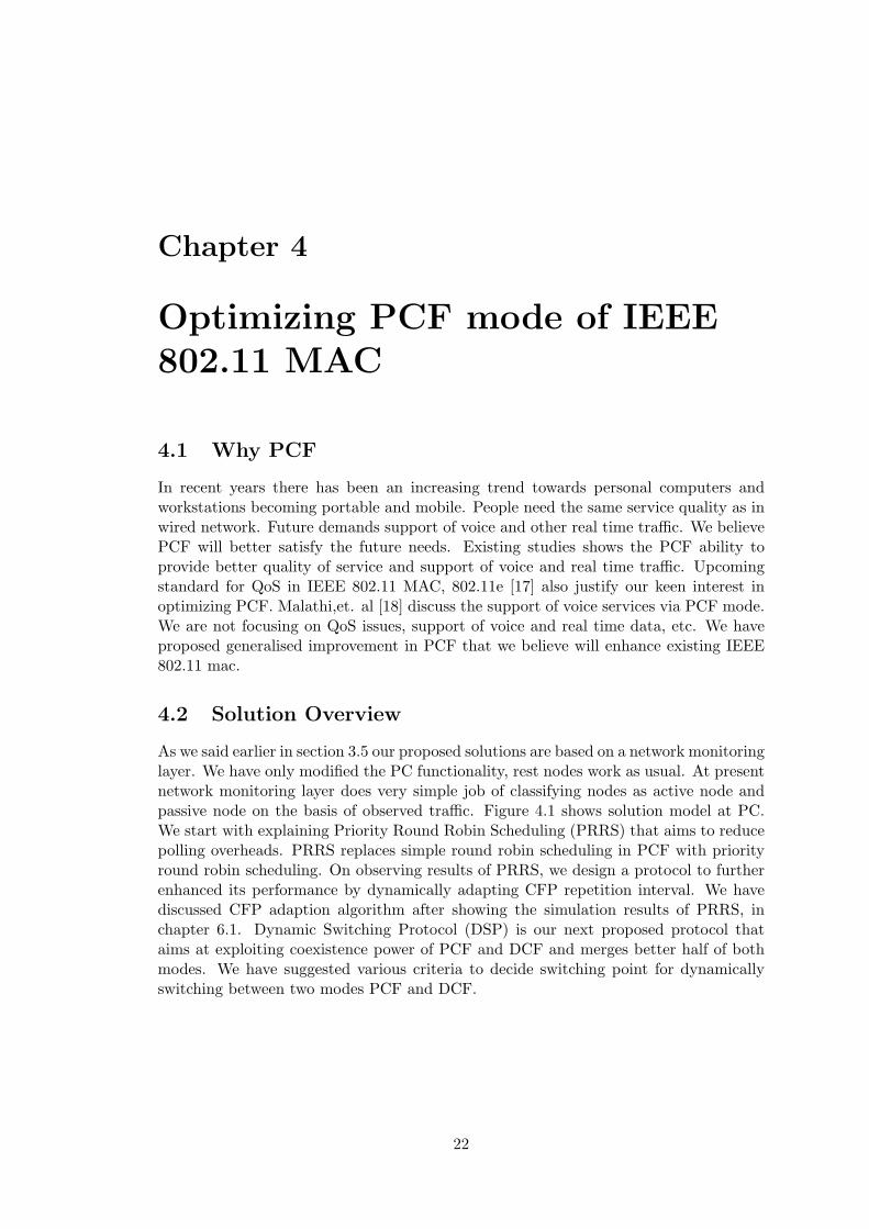
As we said earlier in section 3.5 our proposed solutions are based on a network monitoringlayer. We have only modified the PC functionality, rest nodes work as usual. At presentnetwork monitoring layer does very simple job of classifying nodes as active node andpassive node on the basis of observed traffic. Figure 4.1 shows solution model at PC.We start with explaining Priority Round Robin Scheduling (PRRS) that aims to reducepolling overheads. PRRS replaces simple round robin scheduling in PCF with priorityround robin scheduling. On observing results of PRRS, we design a protocol to furtherenhanced its performance by dynamically adapting CFP repetition interval. We havediscussed CFP adaption algorithm after showing the simulation results of PRRS, inchapter 6.1. Dynamic Switching Protocol (DSP) is our next proposed protocol thataims at exploiting coexistence power of PCF and DCF and merges better half of bothmodes. We have suggested various criteria to decide switching point for dynamicallyswitching between two modes PCF and DCF.
22
4.3 Network Monitoring Layer
Figure 4.1: Solution model at PC
4.3 Network Monitoring Layer
Network Monitor which is PC or access point plays a vital role in both approaches.All stations in BSS need to first associate with PC. PC maintains circular list of allstations associated with it. Root of cause of degraded throughput at low load, whenfew nodes ∗ are speaking, is unsuccessful polling attempts. To avoid such unsuccessfulpolling attempt one needs to have information whether node next in poll list would havedata to transmit or not. Our network monitor PC attempts to do so. It classifies nodeinto distinct categories namely:
• Active Node : Node having high probability to transmit data when being polled.
• Passive Node: Node having low probability to transmit data when being polled.
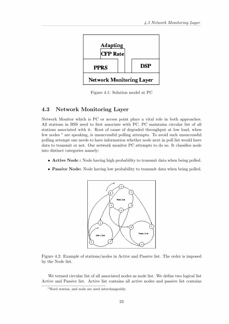
Figure 4.2: Example of stations/nodes in Active and Passive list. The order is imposedby the Node list.
We termed circular list of all associated nodes as node list. We define two logical listActive and Passive list. Active list contains all active nodes and passive list contains
∗Word station, and node are used interchangeably.
23

4.3 Network Monitoring Layer
all passive nodes. Consider figure and assume that stations 1,3, and 5 are classified asactive nodes and may have packet to send. These stations belong to the Active list.Stations 2,4, and 6 are idle nodes and so they belong to passive list. The relative orderin each list is the same as in the node list.
NodeList = ActiveList ∪ PassiveList
ActiveList ∩ PassiveList = Φ
Initially we place all the nodes in active list.
4.3.1 Node List Management
In contention period(CP) of super frame, PC learns node’s activity and at the beginningof each polling round in the next CFP, PC decides which new nodes to be added to activelist. Node list management in contention free period (CFP) is shown in Figure4.3 Everystation on active list retain its position in the list if it transmits data in response to poll.If station does not respond to poll or send null frame then it is termed as passive nodeand placed in passive list. Active node i retains its position as it sends data frame inresponse to poll frame, indicating higher probability of having more data. But node j ismoved to passive list, as its null response reduces its priority.
Figure 4.3: Transmission sequence and list updation in CFP
PC eavesdrops every packet transmitted in the CP and keeps count of number ofdata packets transmitted in CP. Count keeps importance in our DSP approach and itsuse will be discussed later. It examines MAC header to determine frame control typeand subtype. If it is a RTS packet or data packet then PC marks source node as Listennode. Heuristic behind this is very simple. Node transmitting data or RTS packet hashigher probability of sending more data if polled in CFP. In contrast node that remainsilent during entire CP has lesser probability to have data. Obviously second part ofheuristic does hold if CP period is small or node may not get opportunity to transmitor collision occurs, etc. We will discuss this issue in detail later.
Node in passive list remains there if it remain silent in entire CP period. If node inpassive is marked Listen then it is placed in active list for next round of polling.
24
4.4 PRRS-Priority Round Robin Scheduling
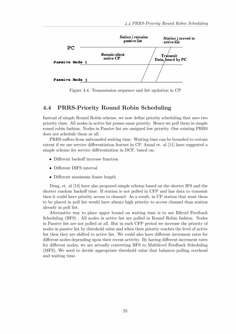
Figure 4.4: Transmission sequence and list updation in CP
4.4 PRRS-Priority Round Robin Scheduling
Instead of simple Round Robin scheme, we now define priority scheduling that uses twopriority class. All nodes in active list posses same priority. Hence we poll them in simpleround robin fashion. Nodes in Passive list are assigned low priority. Our existing PRRSdoes not schedule them at all.
PRRS suffers from unbounded waiting time. Waiting time can be bounded to certainextent if we use service differentiation feature in CP. Amad et. al [11] have suggested asimple scheme for service differentiation in DCF, based on:
• Different backoff increase function
• Different DIFS interval
• Different maximum frame length
Deng, et. al [14] have also proposed simple scheme based on the shorter IFS and theshorter random backoff time. If station is not polled in CFP and has data to transmitthen it could have priority access to channel. As a result, in CP station that want themto be placed in poll list would have always high priority to access channel than stationalready in poll list.
Alternative way to place upper bound on waiting time is to use Bilevel FeedbackScheduling (BFS) . All nodes in active list are polled in Round Robin fashion. Nodesin Passive list are not polled at all. But in each CFP period we increase the priority ofnodes in passive list by threshold value and when their priority reaches the level of activelist then they are shifted to active list. We could also have different increment rates fordifferent nodes depending upon their recent activity. By having different increment ratesfor different nodes, we are actually converting BFS to Multilevel Feedback Scheduling(MFS). We need to decide appropriate threshold value that balances polling overheadand waiting time.
25

4.4 PRRS-Priority Round Robin Scheduling
Algorithm 1: Priority Round Robin Scheduling1: Active list ← ∀0≥i≤N add ni where ni is associated with PC and pollable2: Passive list ←3: if CFP and PC then4: for ni ∈ Active list do5: Poll ni
6: if Recv Null Data Frame or Poll time out then7: Active list ← Active List− ni
8: Passive list ← Passive List + ni
Ensure: Nodes position in logical lists match their corresponding position innode list
9: end if{Actual Implementation may have single node list with boolean param-eter mark don’t poll associated with each node. Set mark don’t poll to true}
10: end for11: else if CP and PC then12: if Listen Packet then13: if Packet.subtype = MAC Subtype RTS or Packet.subtype =
MAC Subtype DATA then14: source node ← Packet.source15: Active list ← Active List + source node16: Passive list ← Passive List− source node17: end if18: end if{Set mark don’t poll to false }19: end if
26
4.5 DSP-Dynamic Switching Protocol
4.5 DSP-Dynamic Switching Protocol
Dynamic switching protocol is defined to exploit the better half of both DCF and PCFmodes. Section 3.2 clears the need of switching protocol. At the broad level, we cansay that in small sized network it is better to use the DCF, otherwise use the PCF.We define network size, not as the total number of nodes in BSS but as the number ofactive nodes. We have network monitoring layer at PC that attempts to approximatethe network size. But it serves our purpose till, we follow the PCF access mode. Sowe need to have some extra mechanism in our existing network monitoring layer toapproximate the network size in DCF mode.
4.6 Learning In DCF
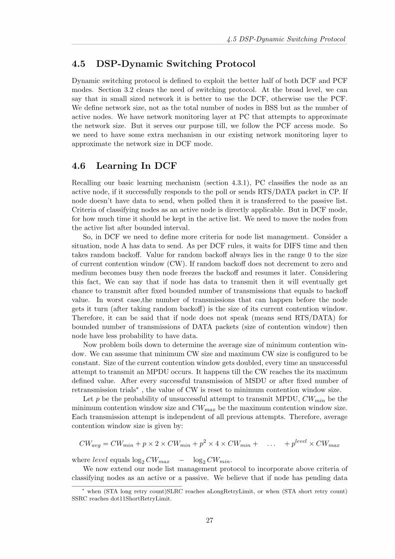
Recalling our basic learning mechanism (section 4.3.1), PC classifies the node as anactive node, if it successfully responds to the poll or sends RTS/DATA packet in CP. Ifnode doesn’t have data to send, when polled then it is transferred to the passive list.Criteria of classifying nodes as an active node is directly applicable. But in DCF mode,for how much time it should be kept in the active list. We need to move the nodes fromthe active list after bounded interval.
So, in DCF we need to define more criteria for node list management. Consider asituation, node A has data to send. As per DCF rules, it waits for DIFS time and thentakes random backoff. Value for random backoff always lies in the range 0 to the sizeof current contention window (CW). If random backoff does not decrement to zero andmedium becomes busy then node freezes the backoff and resumes it later. Consideringthis fact, We can say that if node has data to transmit then it will eventually getchance to transmit after fixed bounded number of transmissions that equals to backoffvalue. In worst case,the number of transmissions that can happen before the nodegets it turn (after taking random backoff) is the size of its current contention window.Therefore, it can be said that if node does not speak (means send RTS/DATA) forbounded number of transmissions of DATA packets (size of contention window) thennode have less probability to have data.
Now problem boils down to determine the average size of minimum contention win-dow. We can assume that minimum CW size and maximum CW size is configured to beconstant. Size of the current contention window gets doubled, every time an unsuccessfulattempt to transmit an MPDU occurs. It happens till the CW reaches the its maximumdefined value. After every successful transmission of MSDU or after fixed number ofretransmission trials∗ , the value of CW is reset to minimum contention window size.
Let p be the probability of unsuccessful attempt to transmit MPDU, CWmin be theminimum contention window size and CWmax be the maximum contention window size.Each transmission attempt is independent of all previous attempts. Therefore, averagecontention window size is given by:
CWavg = CWmin + p× 2× CWmin + p2 × 4× CWmin + . . . + plevel × CWmax
where level equals log2 CWmax − log2 CWmin.We now extend our node list management protocol to incorporate above criteria of
classifying nodes as an active or a passive. We believe that if node has pending data∗ when (STA long retry count)SLRC reaches aLongRetryLimit, or when (STA short retry count)
SSRC reaches dot11ShortRetryLimit.
27

4.7 When to Switch
Figure 4.5: An example of exponential increase of CW
then it will contend for medium and would eventually get chance. to transmit. If nodehas pending data and is contending for medium then it has high probability to getthe chance with in CWavg transmissions. If any active station remains silent for cwavg
transmissions of MPDU in DCF then it is moved to passive list.
Figure 4.6: Extending learning to DCF
4.7 When to Switch
Switching point plays a vital role in DSP. It is very difficult to precisely answer thequestion that ”What should be the optimum point for switching and how to measurethat point?”. We have depicted certain factors that may give some approximation ofswitching point. We will first discuss switching from PCF to DCF and then continuedwith switching from DCF to PCF.
In PCF mode PC being central coordinator, makes the designing of the switchingprotocol little bit easier. It can be assumed that PC can hear every other node in its
28
4.7 When to Switch
BSS. By two ways we can approximate network load and size. First by keeping trackof number of active and passive nodes in the network (refer section 4.3.1). We canalso approximate network load by keeping track of CFP utilization. Details of howto approximate load by CFP utilization can be found in section 6.1. There, we haveused this criteria to dynamically adapt CFP repetition interval. We can also use bothapproaches simultaneously to precise our decision. Here we have used only our firstbasic learning approach.
In DCF mode, things becomes more complicated. How will keep track of node’sactivities, or how many node should do this, Who will be next PC, etc. To simplifythings here, we have used the restricted version of this protocol. We require one fixedpre configured node to act as a PC. PC is made responsible for the network monitoringeven in DCF. Different criteria for approximating load suggested by us are listed below:
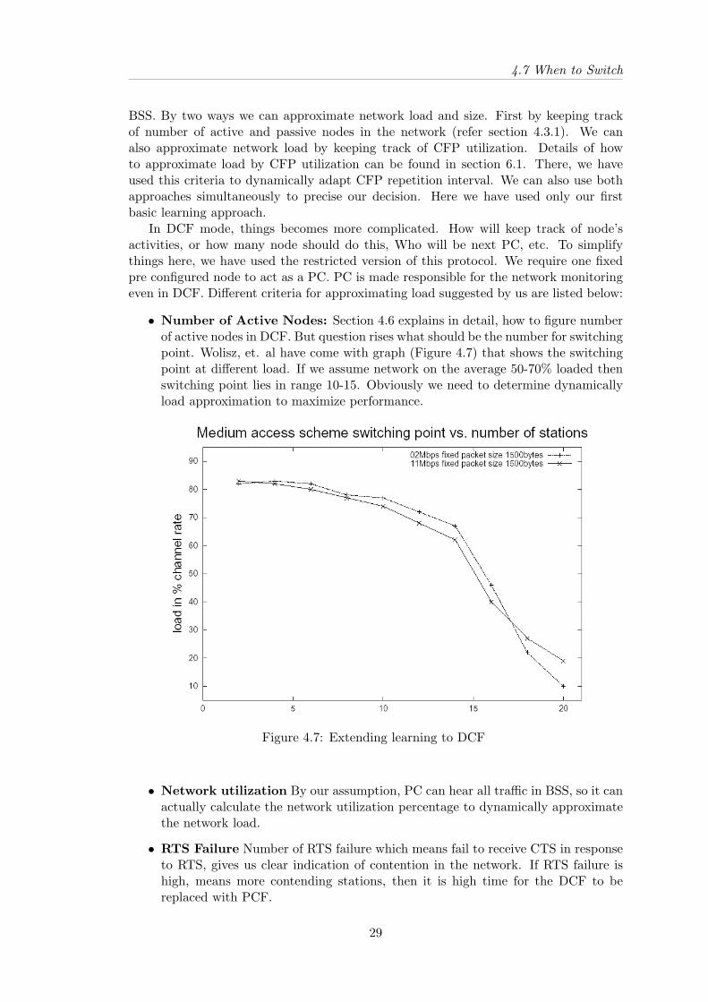
• Number of Active Nodes: Section 4.6 explains in detail, how to figure numberof active nodes in DCF. But question rises what should be the number for switchingpoint. Wolisz, et. al have come with graph (Figure 4.7) that shows the switchingpoint at different load. If we assume network on the average 50-70% loaded thenswitching point lies in range 10-15. Obviously we need to determine dynamicallyload approximation to maximize performance.
Figure 4.7: Extending learning to DCF
• Network utilization By our assumption, PC can hear all traffic in BSS, so it canactually calculate the network utilization percentage to dynamically approximatethe network load.
• RTS Failure Number of RTS failure which means fail to receive CTS in responseto RTS, gives us clear indication of contention in the network. If RTS failure ishigh, means more contending stations, then it is high time for the DCF to bereplaced with PCF.
29

4.8 Restricted DSP
• Number of Collision Assuming center position for PCF, it can hear collisionin its BSS. So we can use the fact to approximate load on the basis of number ofcollision.
Although we have depicted so many criteria for approximating network load, butstill we are not in position to replace all fuzzy decision boundaries with actual switchingpoints. Lots of simulation results and actual experimental data need to be generated,in order come up with good switching points. We decided to stick with graph (Figure4.7) and to use only single criteria of number of active nodes.
4.8 Restricted DSP
Restricted version of DSP, imposes centralization of monitoring and decision makingregarding switching point. Just as the PCF, DSP also needs the central coordinatortermed as PC. PC can regarded as a head of network that decides fate of other station inBSS. All station in BSS needs to be associated with PC just as they do in PCF. This givesus the fair indication of total number of nodes in BSS. Station can change its associationparameters by reassociation request and can also deassociate with deassociation request.Procedure for all these request is same as defined in PCF mode of IEEE 802.11 standard.
Initially network starts in PCF mode. Station associates with PC. PC starts mon-itoring network and decides whether to continue with PCF or switch to DCF. Beacon‘transmissions are scheduled by PC at fixed regular interval.
In PCF mode decision of whether to switch to DCF or not is made at the time ofsending beacon that starts CFP. So after every CFP repetition interval, PC can decideto switch between either modes.
4.8.1 Switching PCF to DCF
Basic intuition behind the protocol is to exploit the virtual carrier sense at the stations inBSS. PC announces CFP by setting the CFP MaxDuration field in the beacon. Stationsin BSS, on the receipt of beacon set their NAV according to the CFP MaxDuration value.This action prevents stations from taking control of the medium during the CFP. If wecan avoid setting of NAV at stations then stations can successfully clear virtual carriersense. Eventually they can take control of medium through DCF access rules. Hencethe network would behave as if, it is in DCF mode. If PC decides to switch to DCFthen following steps are taken:
• Transmit beacon as it do in normal fashion, but with different set of CF parameter.
• Figure 4.8 shows CF parameter set in beacon frame. If PC instead of announcingCFP, want to switch to DCF then set CFMaxDuration, CF DurRemaining andCFP count to non zero high value.
• PC set its CFP count to infinite, set mode ∗ variable DCF and set boolean variablecfp ∗ false.
• PC now doesn’t transmit CFPoll, CF-END, etc.∗ Both variables mode and cfp are required for bookkeeping, not a standard parameter.
30

4.9 Distributed DSP protocol
Figure 4.8: CF parameter set in beacon frame
4.8.2 Switching DCF to PCF
Switching from DCF to PCF uses the same concept of setting NAV that disables thestations to take over medium at the beginning of CFP period. But certain things needto be changed to enable PC and to declare CFP as soon as possible whenever it wantsto switch. In DCF beacon transmission is distributed but in our DSP we have prioritiesPC, such that it is whole and sole responsible for beacon transmission at fixed interval.
Every beacon transmitted in DCF by PC always contains values zero for CFP Max-Duration and CFP DurRemaining. To priorities PC in DCF for transmitting beacons,we have used IFS smaller than DIFS, i.e., PIFS. After PC senses medium free, it needsto wait for only PIFS time instead of DIFS time for other stations. PC decides whetherto switch to PCF or not at the time to send beacon. If PC decides to switch to PCFthen following steps are taken:
• Transmit beacon containing normal values
• PC set its CFP count to its original value(in PCF), set mode variable PCF andset boolean variable cfp true.
• PC now resume its normal functioning, same that it do in PCF after announcingCFP begin.
Bookkeeping helps PC to keep track of its current state. These variables are laterby it decide its functioning.
4.9 Distributed DSP protocol
Distributed version of protocol is designed, keeping in view ad hoc networks. What webelieve that the future advanced IEEE 802.11 LAN card will have both functionalitybuilt in and user will have choice to switch it on or off. Infrastructure need of accesspoint will not be any more. As in ad hoc networks nodes are able to move freely andnetwork size varies a lot. So we believe dynamic switching between either modes wouldgive better performance result and would increase network capacity.
Each node will now monitor the network to keep track of its active neighbours. Whennumber of active neighbours reaches a switching point, then nodes would start to formcluster and runs distributed leader selection algorithm to elect PC among them. Thatnode will then switch on its PCF mode and would take the role of point coordinator.After wards our restricted DSP protocol would take care.
To make whole picture realistic, there exist lots of challenges that needs to be re-solved. Our DSP is first step towards it. Dynamic PC coordinator selection requires aefficient leader selection algorithm that imposes very little overhead. Beside that thereare many security issue regarding association, deassociation with old and new PC, thatneeds to be resolved.
31

Chapter 5
Simulation Results
Our simulations are done using the public domain network simulator NS-2 (2.1b8)[3].Support for wireless simulations in ns was added as a part of the CMU Monarch project[4]. Support for the PCF mode of IEEE 802.11 already exists. [2]. PCF patch addedby Lindgren, et. simulates only limited PCF features. We have simply extended somefeature of existing PCF patch like:
• We added the support for Null data frame that need to be sent in response to poll,if station have no pending data. Previously it was resolved via poll timed out atPC.
• We added support for sending broadcast packet in CFP. Existing implementationsimply drops such packet in CFP
Support for association, deassociation and reassociation still have not been added.Presently nodes need to be associated through tcl script. Since we assume nodes remainin range of PC all the time, therefore static association simply serves our purpose.
5.1 Simulation Setup
Our studies are confined to a single cell of radius 240m, slight less than the transmissionrange of central coordinator. Conceptually every station in region can communicate di-rectly with central node. However, transmission medium degradations due to multipathfading, or interference from nearby BSSs reusing the same physical-layer characteristicscan cause some stations to appear hidden from other stations. In our simulations weare working with only one BSS, a clean channel without errors and fading effects etc.,so all stations can indeed communicate directly with PC.
We have used the default values for all the physical and MAC layer parameters. Thenumber of stations other than PC in circular cell is varied from 8 to 64 asynchronousdata user. Nodes are placed randomly around PC. All our runs are averaged over tensuch random placements. At stations, we attached a cbr source that simulates arrivalof frames for transmission at constant rate. Packet size is kept constant at 500 bytesfor most simulations, except when throughput is studied as a function of packet size.The choice of 500 bytes as a packet size worth studying is motivated by the fact thatwe consider messaging applications to be appropriate for wireless networks.
32

5.2 Simulation Results of PRRS
Parameter ValueTransmission Power 281.8mWTransmission Range 250m
Slot Time 20µs
SIFS 10µs
Channel Bandwidth 2MbpsNumber of Stations Varied from 8 to 64Central Coordinator 1
Packet Size 500 bytesRTS/CTS threshold 250 bytes
Fragmentation threshold 2346 bytesCW Min 31CW Max 1024
CFP repetition interval Varied from 50 to 400 TUsTime Unit (TU) 1024µs
Table 5.1: Simulation Parameters
5.2 Simulation Results of PRRS
We simulated PRRS for 300 seconds using different traffic loads and network size. Nodesplacement is total random. In all simulations for PRRS, we have changed the sourcesdynamically. Consider graph in figure 5.1, we have three different set of 8 sources.Source nodes of each set send packets for 100 seconds. All 8 cbr sources start and endat same time.
5.2.1 Throughput
We define throughput as the total number of bits per second passed up from the MACsublayer at each destination. Then we present it as a fraction of channel bandwidth. Sothe throughput what we measure here is actually the goodput, because control frames,management frames,routing packets, header size, etc. are not counted. Similarly, weoffered load as the average number of bits per second of actual data offered to the MACsublayer at each source. It is then represented as a fraction of channel bandwidth.
Figure 5.1 shows PRRS result with 25% node active and total 32 nodes in BSS.Highest throughput achieved by PRRS is 0.637534 × 2000000 = 1275068 bps and withRRS is 0.585006×2000000 = 1170012 bps. Around 10% increase in goodput is achieved.Considering the same ratio of active nodes and total nodes, with 64 nodes (figure 5.2Throughput difference is highest when offered load is 80%. Throughput achieved byPCF with RRS at 80% offered load is 0.511695 × 2000000 = 1023390 bps and by PCFwith PRRS is 0.592234 × 2000000 = 1184460 bps. Throughput improved by 15.7%approximately.
33

5.2 Simulation Results of PRRS
Figure 5.1: Throughput Comparison between PCF with PRRS and non optimized PCFwith RRS. Total node =32 and 25% active node
Figure 5.2: Throughput Comparison between PCF with PRRS and non optimized PCFwith RRS. Total node =64 and 25% active node
Figure 5.3 shows the throughput comparison with 32 nodes and among them 50%75%100% active. As number of active nodes increases throughput difference decreases.Figure 5.4 shows the throughput comparison with 64 nodes and among them 50% and75% active.
34

5.2 Simulation Results of PRRS
(a) 50% Active nodes
(b) 75% Active nodes (c) 100% Active nodes
Figure 5.3: Throughput comparison of PRRS against non optimized PCF with 32 nodes
(a) 50% Active nodes (b) 75% Active nodes
Figure 5.4: Throughput comparison of PRRS against non optimized PCF with 64 nodes
35
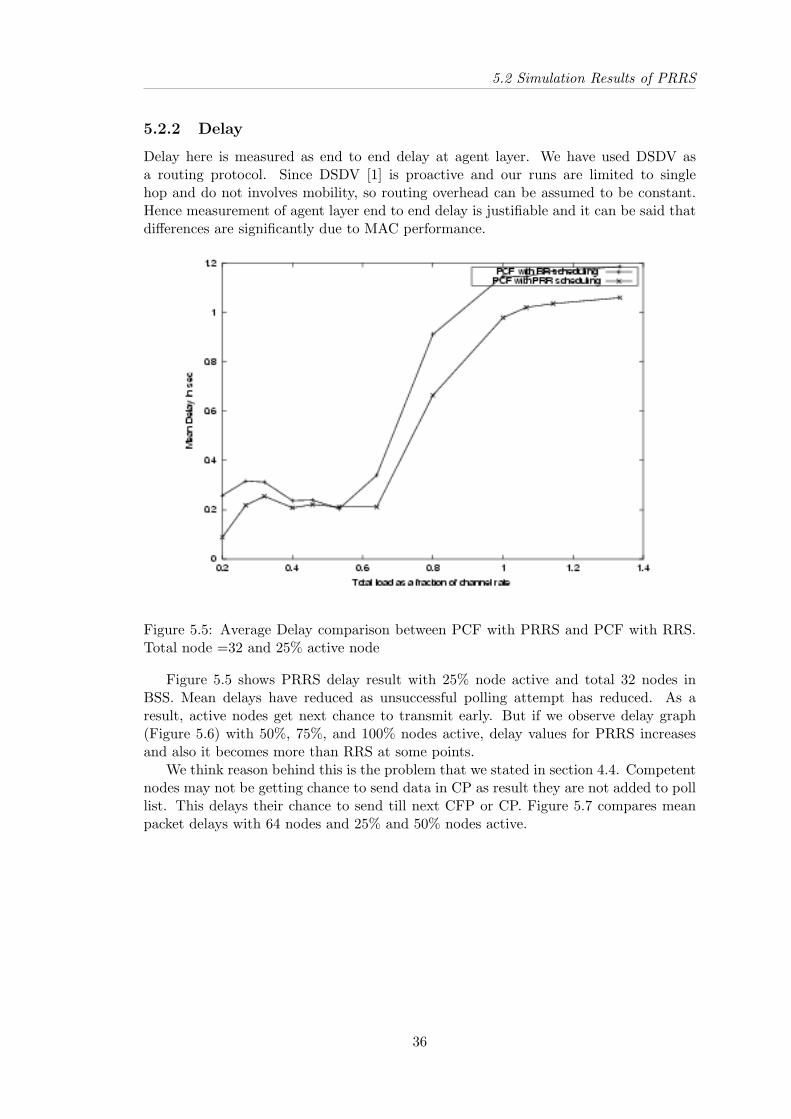
5.2 Simulation Results of PRRS
5.2.2 Delay
Delay here is measured as end to end delay at agent layer. We have used DSDV asa routing protocol. Since DSDV [1] is proactive and our runs are limited to singlehop and do not involves mobility, so routing overhead can be assumed to be constant.Hence measurement of agent layer end to end delay is justifiable and it can be said thatdifferences are significantly due to MAC performance.
Figure 5.5: Average Delay comparison between PCF with PRRS and PCF with RRS.Total node =32 and 25% active node
Figure 5.5 shows PRRS delay result with 25% node active and total 32 nodes inBSS. Mean delays have reduced as unsuccessful polling attempt has reduced. As aresult, active nodes get next chance to transmit early. But if we observe delay graph(Figure 5.6) with 50%, 75%, and 100% nodes active, delay values for PRRS increasesand also it becomes more than RRS at some points.
We think reason behind this is the problem that we stated in section 4.4. Competentnodes may not be getting chance to send data in CP as result they are not added to polllist. This delays their chance to send till next CFP or CP. Figure 5.7 compares meanpacket delays with 64 nodes and 25% and 50% nodes active.
36

5.2 Simulation Results of PRRS
(a) 50% Active nodes
(b) 75% Active nodes (c) 100% Active nodes
Figure 5.6: Delay Graphs with 32 nodes and among them 50%, 75%, and 100% active.
(a) 25% Active nodes (b) 50% Active nodes
Figure 5.7: Delay Graphs with 64 nodes and among them 25% and 50% active
37

5.3 Simulation Results of DSP
5.3 Simulation Results of DSP
We simulated DSP for 350 seconds. We changed the traffic pattern for DSP simulation.Previously all cbr connection starts and ends at same instant of time but now we haveintroduced 1ms time gap between starting time of cbr connections. We have placednodes randomly and averaged the reading over 10 such random placements. Switchingpoint used by us is:
• DCF till number of active nodes less than equal to 10.
• PCF when number of active nodes exceeds 10.
Figure 5.8: Throughput comparison of DSP with PCF and DCF
Graph shown in figure 5.8 shows the throughput comparison of DSP with PCF and DCFmode. We simulated with 16 nodes in BSS. Number of active nodes is varied form 4 to16. Traffic load is defined as
• From 0 to 50 sec, we have 4 cbr connections
• From 51 to 100 sec, we have 8 cbr connections
• From 101 to 150 sec, we have 12 cbr connections
• From 151 to 200 sec, we have 16 cbr connections
• From 201 to 250 sec, we have 11 cbr connections
• From 251 to 300 sec, we have 7 cbr connections
• From 301 to 351 sec, we have 4 cbr connections
On x-axis we have varied packet inter arrival time from 200 ms to 10 ms. Resultshows the throughput improvements on using DSP. Graph in figure 5.9 shows the delaycurve for DSP. DSP offers lower mean packet delays than both PCF and DCF.
38

5.4 Result Summary
Figure 5.9: Delay comparison of DSP with PCF and DCF
5.4 Result Summary
PRRS shows better results than PCF with RRS, especially when less than 75% nodehave pending data to send. It suffers from higher delays when percentage of active nodesreaches 75% and more. We have discussed possible reason for this in section 4.4. DSPrequires extensive experimentations. We have seen improvements in both throughputand mean delay.
We have used different CFP repetition intervals, while experimenting with PRRS.We varied the parameter in accordance with number of nodes in network. In nextchapter we will show effect of this parameter on PCF performance.
39

Chapter 6
Adapting CFP under varyingLoad
In this chapter we concentrate on the dynamic adaption of CFP repetition interval.Basic intuition behind the use of different CFP repetition interval in our simulations(Section 5.2) for different number of nodes in network,is to poll nodes in CFP exactlyonce and to have enough CP period left for the PC to learn nodes activity. So thatmore more competing station can be added to active list. Big CFP repetition intervalimplies large CFP Max duration. After single round of polling, PC transmits CF Endand starts the CP that lasts till the next CFP. Large CP, no doubt gives the PC moretime to examine nodes activity but network remains in DCF mode for that longer period.
Similarly small CFP repetition interval implies small CFP Max duration. So, it mayhappen that PC may not be able to poll all active nodes at least once. CP period is alsoless because whole CFP max may be utilized. This reduces the chance for competingstations to get enrolled in active list. Hence stations are polled after longer delays. Westatically calculated CFP repetition interval for our runs. Let total number of nodesin network be 32 and mean packet size be 500 bytes. Time require to poll all stationsassuming each will have data to send is:-
Total T ime = 32 ∗ TP oll
= 32 ∗ 3SIFS + TCFpoll + TData
= 32 ∗ 2.5TUs
= 80TUs
It takes 80 TUs to poll all 32 stations. Hence, we took CFP repetition interval as100 TUs for such scenario.
In short, arbitrary chosen value for CFP repetition interval may deviate performancefar from achievable Effect of CFP repetition interval on throughput can be properlyanalysed from graphs. Simulation setup is same as we described in section 5.1.Graph 6.1shows that with 32 active nodes better throughput is achieved when CFP repetitioninterval is 100 TUs. At peak load story is slightly different. CFP repetition intervalequals 50 TUs gives better throughput than rest. We think more throughput value maybe because, nodes always have data to send, so low CFP repetition interval like 50 TUsallows to poll at lower delays. But we think that it may cause unfairness with otherstations. Since network remains in CP for less time, so other competent nodes get lesstime to get enrolled in active list while stations in active list get polls at lower delay.
40

Figure 6.1: Throughput in PCF with PRRS for different CFP repetition interval with32 active nodes
We need to noted that there is high variation in throughput by changing just singleconfiguration parameter (CFP repetition interval). At 70% load, throughput acheivedwith CFP repetition interval equals 100 TUs is approximately 61.5% and with 400 TUsit is only 52.8%. This clearly justifies our argument of dynamic adaption.
(a) 16 Active nodes (b) 64 Active nodes
Figure 6.2: Throughput in PCF with PRRS for different CFP repetition interval with8,16 and 64 active nodes.
As the number of active nodes changes, better CFP repetition interval value varies.Graphs in figure 6.2 shows the dependence of good value on the number of active nodes.Same arguments holds for the delay values. Graph in figure 6.3 shows the delay curves
41

6.1 CFP Adaption
(a) 16 Active nodes
(b) 32 Active nodes (c) 64 Active nodes
Figure 6.3: Mean packet delays in PCF with PRRS for different CFP repetition intervalwith 8,16 and 64 active nodes.
for different number of active nodes.
6.1 CFP Adaption
Standard states that each beacon transmitted during CFP or starts CFP, always containsinformation regarding the remaining CFP duration or CFP max duration respectively.Stations hearing beacon, set their NAV according to announced CFP duration. Weutilize this fact to further optimize PRRS and dynamically adapt CFP repetition intervalunder varying load. Our solution to dynamically adapt CFP repetition interval is alsoapplicable to PCF with RRS.
Although we have notion of number of active nodes in network but assumption ofaverage packet size may not be correct. So statically calculated CFP repetition intervalmay not be optimal. We take different path of measuring CFP utilization to definenew CFP repetition interval. Basic purpose is to keep to keep the network in CFP formaximum possible time and to ensure fairness for passive nodes by having enough CPlength and CP repetition interval.
42
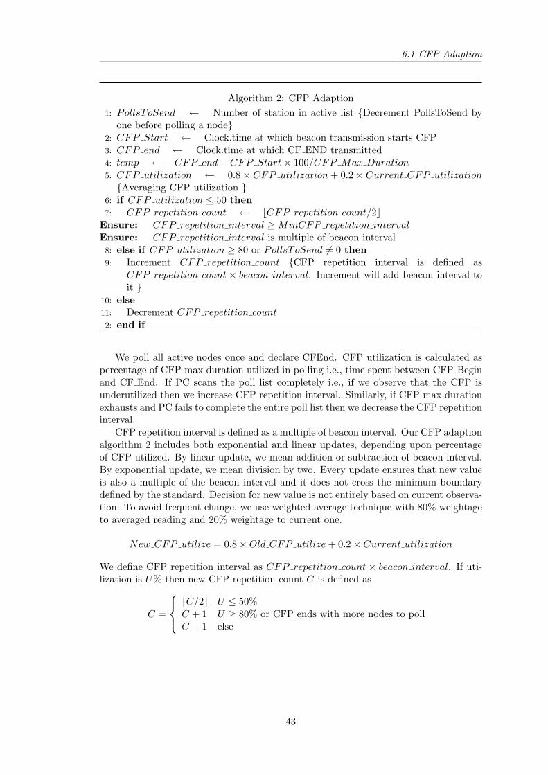
6.1 CFP Adaption
Algorithm 2: CFP Adaption1: PollsToSend ← Number of station in active list {Decrement PollsToSend by
one before polling a node}2: CFP Start ← Clock.time at which beacon transmission starts CFP3: CFP end ← Clock.time at which CF END transmitted4: temp ← CFP end− CFP Start× 100/CFP Max Duration5: CFP utilization ← 0.8× CFP utilization + 0.2× Current CFP utilization{Averaging CFP utilization }
6: if CFP utilization ≤ 50 then7: CFP repetition count ← bCFP repetition count/2c
Ensure: CFP repetition interval ≥MinCFP repetition intervalEnsure: CFP repetition interval is multiple of beacon interval8: else if CFP utilization ≥ 80 or PollsToSend 6= 0 then9: Increment CFP repetition count {CFP repetition interval is defined as
CFP repetition count× beacon interval. Increment will add beacon interval toit }
10: else11: Decrement CFP repetition count12: end if
We poll all active nodes once and declare CFEnd. CFP utilization is calculated aspercentage of CFP max duration utilized in polling i.e., time spent between CFP Beginand CF End. If PC scans the poll list completely i.e., if we observe that the CFP isunderutilized then we increase CFP repetition interval. Similarly, if CFP max durationexhausts and PC fails to complete the entire poll list then we decrease the CFP repetitioninterval.
CFP repetition interval is defined as a multiple of beacon interval. Our CFP adaptionalgorithm 2 includes both exponential and linear updates, depending upon percentageof CFP utilized. By linear update, we mean addition or subtraction of beacon interval.By exponential update, we mean division by two. Every update ensures that new valueis also a multiple of the beacon interval and it does not cross the minimum boundarydefined by the standard. Decision for new value is not entirely based on current observa-tion. To avoid frequent change, we use weighted average technique with 80% weightageto averaged reading and 20% weightage to current one.
New CFP utilize = 0.8×Old CFP utilize + 0.2× Current utilization
We define CFP repetition interval as CFP repetition count × beacon interval. If uti-lization is U% then new CFP repetition count C is defined as
C =
bC/2c U ≤ 50%C + 1 U ≥ 80% or CFP ends with more nodes to pollC − 1 else
43

6.2 Simulation Results
6.2 Simulation Results
We have used same simulation scenario as used in section 5.2. Figure 6.4 shows theperformance of CFP adaption enabled PCF. It adapts very well at moderate load, andthe delay characteristics (fig. 6.5) have also improved.
Figure 6.4: Throughput comparison of PCF with PRRS for different CFP repetitioninterval with CFP adaption enabled PCF with PRRS
Figure 6.5: Delay characteristic of PCF with PRRS for different CFP repetition intervalwith CFP adaption enabled PCF with PRRS
Figure 6.6 shows results with 8 and 16 nodes active. Their delay characteristic are shownin figure 6.7
44
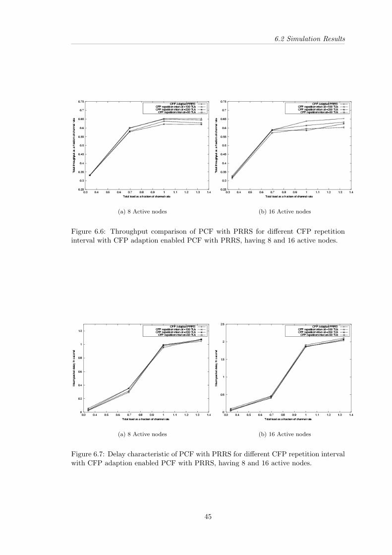
6.2 Simulation Results
(a) 8 Active nodes (b) 16 Active nodes
Figure 6.6: Throughput comparison of PCF with PRRS for different CFP repetitioninterval with CFP adaption enabled PCF with PRRS, having 8 and 16 active nodes.
(a) 8 Active nodes (b) 16 Active nodes
Figure 6.7: Delay characteristic of PCF with PRRS for different CFP repetition intervalwith CFP adaption enabled PCF with PRRS, having 8 and 16 active nodes.
45
Chapter 7
Conclusion and Future Research
7.1 Conclusion
IEEE 802.11 MAC needs dynamic adaption to enhance its performance. Static con-figured MAC performance deviates a lot from achievable limit. We have suggesteda network monitoring based approaches to approximate the network sizeand load and dynamically adapt MAC. Our approaches add very little overheadand strictly follows the standard, without demanding any change in existing frame for-mats and access procedures. The best thing about our approaches is that, they addjust one additional network monitoring layer at access point (PC) and rest all stationsfunctionality remain unchanged.
PRRS that replaces simple round robin scheduling in PCF, significantly overcomesthe efficiency of the polling schemes especially when small fraction of stations have datato transmit and when the traffic load is moderate. We have achieved around 10% to15% improvement in throughput. By reducing unsuccessful polling attempts when fewnodes in BSS have data to transmit, it reduces mean packet delays. This makes it moresuitable for handling real time data and multimedia traffic.
DSP that defines protocol for dynamic switching between PCF and DCF, opens anew door to exploit coexistence of DCF and PCF mode and to mix better half of boththe modes. We have also provided various ways to approximate size and traffic load, fordefining ideal switching point. Our idea of distributed DSP would increase the networkcapacity and enhance performance in an ad hoc networks.
We have showed the need for dynamic adaption of CFP repetition interval for en-suring both better throughput and the fairness. Around 10-20% throughput variationis observed by using different configuration. Our CFP Adaption protocol success-fully adapt CFP rate to suit current network load. CFP adapted PCF has achievedperformance almost close to or even better than statically configured PCF.
7.2 Future Research
Our current version of PRRS introduces slight more delays for some nodes, when numberof active nodes ∗ approaches total number of nodes. We need to implement servicedifferentiation mechanism to priorities nodes that have not been polled in CFP, to senddata packet in CP. There is need to explore alternative Bilevel feedback scheduling policy(Section 4.4). Whether Bilevel feedback scheduling is sufficient, when we need multiple
∗nodes have data to transmit
46
7.2 Future Research
feedback scheduling, how to adjust number of levels in feedback scheduling dynamicallydepending upon current traffic load and network size, etc., are still open for researchand further experimentation.
Restricted version of DSP needs better approximation of traffic load to define switch-ing point. We have suggested various alternative for that, but there is need to extensivelyexplore these options and do rigorous experiments. Designing the distributed version ofDSP is a great challenge in itself. It require robust protocol for clustering of nodes andPC selection. Many security related issues ∗ need to be resolved for deploying distributedDSP.
CFP Adaption algorithm is just a first step towards dynamic adaption of configura-tion parameters. Algorithm needs to be refined further. Using the network monitoringlayer, we need to design protocol for adapting other configuration parameters like min-imum CW size, RTS/CTS threshold,etc.
∗Regarding association and deassociation with newly selected PC
47
Bibliography
[1] Charles E. Perkins, Pravin Bhagwat, Highly dynamic Destination-SequencedDistance-Vector routing (DSDV) for mobile computers, ACM SIGCOMM ComputerCommunication Review, v.24 n.4, p.234-244, Oct. 1994.
[2] Anders Lindgren and Andreas Almquist, Implementation of the PCF mode ofIEEE 802.11 for the NS-2 Network Simulator, http://www.sm.luth.se/ dug-dale/index/software.shtml
[3] The VINT project, NS notes and documentation, editors Kevin Fall and Kan-nan Varadhan, http://www.isi.edu/nsnam/ns
[4] Josh Broch, David A. Maltz David B. Johnson,Yih-Chun Hu and Jorjeta Jetcheva,A Performance Comparison of Multi-hop Wireless ad hoc Networking Routing Pro-tocols, Proceedings of Mobicom,October 1998.
[5] Shugong Xu, Tarek Saadawi Does IEEE 802.11 MAC Protocol Work Well in Multi-hop Wireless Ad Hoc Networks?, IEEE Communications Magazine, p.130-137, June2001.
[6] Andreas Kopsel, Jean-Pierre Ebert, and Adam Wolisz, A Performance Comparisonof Point and Distributed Coordination Function of an IEEE 802.11 WLAN in thepresence of Real-Time Requirements, Proc. of 7th Intl. Workshop on Mobile Multi-media Communications (MoMuC2000), October 23-26, 2000.
[7] Leena Chandran-Wadia, Shruti M. and Sridhar Iyer. Throughput Performance of theDistributed and Point Coordination Functions of an IEEE 802.11 Wireless LAN ,ICCC’2002, Aug. 11-4, Mumbai, India
[8] Brian P. Crowe, I. Widjaja, J. Kim, P. Sakai, IEEE 802.11 Wireless Local AreaNetworks, IEEE Communications Magazine, September 1997.
[9] Vaduvur Bharghavan, Alan Demers, Scott Shenker and Lixia Zhang. MACAW: amedia access protocol for wireless LAN’s in Proc. ACM SIGCOMM ’94, pp. 212-25,London, UK, Aug. 31–Sept. 2, 1994.
[10] IEEE Std. 802.11, Wireless LAN Media Access Control (MAC) and Physical Layer(PHY) Specifications, 1999.
[11] I. Aad and C. Castelluccia. Differentiation mechanisms for IEEE 802.11 In Pro-ceedings of IEEE INFOCOM 01,Anchorage, Alaska, April 2001.
[12] Frederico Cal̀ı, Marco Conti, and Enrico Gregori Dynamic tuning of the IEEE802.11 protocol to achieve a theoretical throughput limit, IEEE /ACM Transactionson Networking, 8(6):785-799, 2000.
48

BIBLIOGRAPHY
[13] Harshal S. Chhaya and Sanjay Gupta. Performance modeling of asynchronous datatransfer methods of IEEE 802.11 mac protocol, Wireless Networks,3(3):217-234,1997.
[14] J. Deng and R. Chang. “A priority scheme for IEEE 802.11 DCF access method”IEICE Trans. Comm. E82-B, (1): 96-102, Jan. 1999.
[15] Oran Sharon, Eitan Altman An efficient polling MAC for Wireless LANsIEEE/ACM Transactions on Networking 9(4):439-451, (2001).
[16] Ravindra S. Ranasinghe, Lachlan L. H. Andrew, and David Everitt, Impact ofpolling strategy on capacity of 802.11 based wireless multimedia LANs. In Proc. IEEEInt. Conf. On Networks ICON,Brisbane, Australia, 1999.
[17] P. May, O. Klein, G. Hiertz, S. Mangold, S. Choi and L. Stibor, IEEE 802.11ewireless LAN for quality of service (invited paper), In Proceedings of the EuropeanWireless, volume 1, pages 32-39, Florence, Italy, February 2002.
[18] Malathi Veeraraghavan, Nabeel Cocker, and Tim Moors: Support of voice servicesin IEEE 802.11 wireless LANs. INFOCOM 2001 : 488-497
[19] Matthijs A. Visser and Magda El Zarki Voice and data transmission over an 802.11wireless network. Proceedings of the 6th IEEE International Symposium on Personal,Indoor and Mobile Radio Communications, PIMRC’95, pages 648-652, Sept. 27-291995.
[20] J.Weinmiller, H.Woesner, J. P. Ebert, and A.Wolisz. Analyzing and tuning theDistributed Coordination Function in the IEEE 802.11 DFWNAC draft standard.MASCOT,San Jose, CA, Feb. 1996.
[21] Jost Weinmiller, Morten Schlger, Andreas Festag, and Adam Wolisz. Performancestudy of access control in wireless LANS IEEE 802.11 DFWMAC and ETSI RES10 Hiperlan, Mobile Networks and Applications, 2(1):55-67, 1997.
49