durrani thesis
TRANSCRIPT

Investigations into Smart Antennas forCDMA Wireless Systems
by
Salman Durrani
A thesis submitted in theSchool of Information Technology & Electrical Engineering
in fulfillment of the requirementsfor the degree of
Doctor of Philosophy
at the
The University of Queensland,Brisbane, Australia.
August 2004

Investigations into Smart Antennas for CDMA Wireless Systems
Copyright c© 2004 by Salman Durrani.
All Rights Reserved.
This thesis is dedicated to my parents, Karam Elahi Durrani and Samia Durrani, to whom
I owe my love of learning.


Statement of Originality
The work presented in the thesis is, to the best of my knowledge and belief, original and my
own work except as acknowledged in the text. The material has not been submitted, either
in whole or in part, for a degree at the University of Queensland or any other university.
Salman Durrani
August 2004
v


Abstract
Over the last few years, wireless cellular communications has experienced rapid growth in
the demand for provision of high data rate wireless multimedia services. This fact motivates
the need to find ways to improve the spectrum efficiency of wireless communication sys-
tems. Smart or adaptive antennas have emerged as a promising technology to enhance the
spectrum efficiency of present and future wireless communications systems by exploiting
the spatial domain. The aim of this thesis is to investigate smart antenna applications for
Direct Sequence Code Division Multiple Access (DS-CDMA) systems. CDMA is chosen
as the platform for this thesis work since it has been adopted as the air-interface technology
by the Third Generation (3G) wireless communication systems.
The main role of smart antennas is to mitigate Multiple Access Interference (MAI) by
beamforming (i.e. spatial filtering) operation. Therefore, irrespective of a particular wire-
less communication system, it is important to consider whether a chosen array configuration
will enable optimal performance. In this thesis an initial assessment is carried out consid-
ering linear and circular array of dipoles, that can be part of a base station antenna system.
A unified and systematic approach is proposed to analyse and compare the interference
rejection capabilities of the two array configurations in terms of the Signal to Interference
Ratio (SIR) at the array output. The theoretical framework is then extended to include the
effect of mutual coupling, which is modelled using both analytical and simulation methods.
Results show that when the performance is averaged over all angles of arrival and mutual
coupling is negligible, linear arrays show similar performance as circular arrays. Thus in
the remaining part of this thesis, only linear arrays are considered.
In order to properly evaluate the performance of smart antenna systems, a realistic chan-
nel model is required that takes into account both temporal and spatial propagation char-
vii

acteristics of the wireless channel. In this regard, a novel parameterized physical channel
model is proposed in this thesis. The new model incorporates parameters such as user mo-
bility, azimuth angle of arrival, angle spread and Doppler frequency, which have critical
influence on the performance of smart antennas. A mathematical formulation of the chan-
nel model is presented and the proposed model is implemented in software using Matlab.
The statistics of the simulated channels are analysed and compared with theory to confirm
that the proposed model can accurately simulate Rayleigh and Rician fading characteristics.
To assist system planners in the design and deployment of smart antennas, it is important
to develop robust analytical tools to assess the impact of smart antennas on cellular systems.
In this thesis an analytical model is presented for evaluating the Bit Error Rate (BER) of
a DS-CDMA system employing an array antenna operating in Rayleigh and Rician fading
environments. The DS-CDMA system is assumed to employ noncoherentM-ary orthog-
onal modulation, which is relevant to IS-95 CDMA and cdma2000. Using the analytical
model, an expression of the Signal to Interference plus Noise Ratio (SINR) at the output
of the smart antenna receiver is derived, which allows the BER to be evaluated using a
closed-form expression. The proposed model is shown to provide good agreement with
the (computationally intensive) Monte Carlo simulation results and can be used to rapidly
calculate the system performance for suburban and urban fading environments.
In addition to MAI, the performance of CDMA systems is limited by fast fading. In
this context, a hybrid scheme of beamforming and diversity called Hierarchical Beamform-
ing (HBF) is investigated in this thesis to jointly combat MAI and fading. The main idea
behind HBF is to divide the antenna elements into widely separated groups to form sub-
beamforming arrays. The performance of a hierarchical beamforming receiver, applied
to an IS-95 CDMA system, is compared with smart antenna (conventional beamforming)
receiver and the effect of varying the system and channel parameters is studied. The sim-
ulation results show that the performance of hierarchical beamforming is sensitive to the
operating conditions, especially the value of the azimuth angle spread.
The work presented in this thesis has been published in part in several journals and
refereed conference papers, which reflects the originality and significance of the thesis con-
tributions.
viii

Acknowledgements
First, I would like to express my deepest appreciation and sincerest gratitude to my advisor,
Prof. Dr. Marek E. Bialkowski, for his encouragement, advice and generous financial
support during the course of my PhD. This thesis would not have been possible without his
invaluable technical insight and continuous guidance.
I would like to thank all my senior colleagues at the University of Queensland, in par-
ticular Dr. John Homer, Dr. Nicholas Shuley and Prof. John L. Morgan (Warden, St John’s
College) for their advice. I thank my office mates and PhD colleagues Eddie Tsai, Januar
Janapsatya and Serguei Zagriatski for their enjoyable company and discussions, both tech-
nical and non-technical. Many thanks are also due to Mr. Richard Taylor (School Technical
Infrastructure Manager) for providing the extra computer systems support and facilities for
the simulation work in the thesis.
Special thanks are due to Emad Abro and Ishaq Burney for their friendship and sense
of humour which kept me sane over the past three and a half years.
I would like to acknowledge the support of the Australian government and the School of
Information Technology & Electrical Engineering (ITEE), The University of Queensland,
Brisbane, for provision of an International Postgraduate Research Scholarship (IPRS) and
a School of ITEE International Scholarship respectively.
Last but not the least, I would like to thank my family; my sisters Sarah and Sameera
for their love and patience and my parents for their continuous encouragement and moral
support.
ix


Thesis Publications
The work presented in this thesis has been published, in part, in the following journals and
refereed conference proceedings:-
Refereed Journal Papers
• S. Durrani and M. E. Bialkowski, “Analysis of the error performance of adaptive ar-
ray antennas for CDMA with noncoherentM-ary orthogonal modulation in nakagami
fading,” to appear in IEEE Communications Letters, vol. 9, no. 2, Feb. 2005.
• S. Durrani and M. E. Bialkowski, “Effect of mutual coupling on the interference
rejection capabilities of linear and circular arrays in CDMA systems,”IEEE Trans-
action on Antennas and Propagation, vol. 52, no. 4, pp. 1130-1134, Apr. 2004.
• S. Durrani and M. E. Bialkowski, “An investigation into the interference rejection
capability of a linear array in a wireless communications system,”Microwave and
Optical Technology Letters, vol. 35, no. 6, pp. 445-449, Dec. 2002.
• S. Durrani and M. E. Bialkowski, “Interference rejection capabilities of different
types of antenna arrays in cellular systems,”IEE Electronics Letters, vol. 38, pp.
617-619, June 2002.
Refereed International Conference Papers
• S. Durrani and M. E. Bialkowski, “A simple model for performance evaluation of
a smart antenna in a CDMA system,” inProc. IEEE International Symposium on
Spread Spectrum Techniques and Applications (ISSSTA), Sydney, Australia, Aug. 30
- Sep. 2, 2004, pp. 379-383.
• S. Durrani and M. E. Bialkowski, “Performance of hierarchical beamforming in a
xi

Rayleigh fading environment with angle spread,” inProc. International Symposium
on Antennas (ISAP), vol. 2, Sendai, Japan, Aug. 17-21, 2004, pp. 937-940.
• S. Durrani and M. E. Bialkowski, “Effect of angular energy distribution of an inci-
dent signal on the spatial fading correlation of a uniform linear array,” inProc. Inter-
national Conference on Microwaves, Radar and Wireless Communications (MIKON),
vol. 2, Warsaw, Poland, May 17-19, 2004, pp. 493-496.
• S. Durrani and M. E. Bialkowski, “Performance analysis of beamforming in ricean
fading channels for CDMA systems,” inProc. Australian Communications Theory
Workshop (AusCTW), Newcastle, Australia, Feb. 4-6, 2004, pp. 1-5.
• S. Durrani and M. E. Bialkowski, “A smart antenna model incorporating an az-
imuthal dispersion of received signals at the base station of a CDMA system,” in
Proc. IEEE International Multi Topic Conference (INMIC), Islamabad, Pakistan,
Dec. 8-9, 2003, pp. 218-223.
• S. Durrani and M. E. Bialkowski, “BER performance of a smart antenna system for
IS-95 CDMA,” in Proc. IEEE International Symposium on Antennas and Propaga-
tion (AP-S), vol. 2, Columbus, Ohio, June 22-27, 2003, pp. 855-858.
• S. Durrani and M. E. Bialkowski, “Simulation of the performance of smart anten-
nas in the reverse link of CDMA system,” inProc. IEEE International Microwave
Symposium (IMS), vol. 1, Philadelphia, Pennsylvania, June 8-13, 2003, pp. 575-578.
• S. Durrani, M. E. Bialkowski and J. Janapsatya, “Effect of mutual coupling on the
interference rejection capabilities of a linear array antenna, ” inProc. Asia Pacific
Microwave Conference (APMC), vol. 2, Kyoto, Japan, Nov. 19-22, 2002, pp. 1095-
1098.
• S. Durrani and M. E. Bialkowski, “Investigation into the performance of an adaptive
array in cellular environment,” inProc. IEEE International Symposium on Antennas
and Propagation (AP-S), vol. 2, San Antonio, Texas, June 16-21, 2002, pp. 648-651.
• S. Durrani and M. E. Bialkowski, “Development of CDMASIM: a link level simu-
lation software for DS-CDMA systems,” inProc. 14th International Conference on
Microwaves, Radar and Wireless Communications (MIKON), Gdansk, Poland, May
20-22, 2002, pp. 861-864.
xii

National Conference Abstracts
• S. Durrani and M. E. Bialkowski, “Influence of mutual coupling on the interfer-
ence rejection capability of a smart antenna system,”8th Australian Symposium on
Antennas (ASA), Sydney, pp. 20, Feb. 12-13, 2003.
• S. Durrani and M. E. Bialkowski, “The performance of a smart antenna system in
multipath fading environment for CDMA,”4th Australian Communications Theory
Workshop (AusCTW), Melbourne, pp. 10, Feb. 5-7, 2003.
Project Awards
• Highly Commended Student Presentation Award, Eighth Australian Symposium
on Antennas, CSIRO Telecommunications & Industrial Physics Centre, Sydney, Aus-
tralia, Feb. 2003.
(one first prize and two honourable mention prizes were awarded at the conference.)
• Richard Jago Memorial Prize, School of Information Technology & Electrical En-
gineering, The University of Queensland, 2001.
(prize awarded for the purpose of furthering research by attendance at a conference.)
xiii

Contents
Statement of Originality v
Abstract vii
Acknowledgements ix
Thesis Publications xi
List of Figures xxi
List of Tables xxv
List of Abbreviations xxvii
List of Symbols xxix
1 Introduction 1
1.1 Background . . . . . . . . . . . . . . . . . . . . . . . . . . . . . . . . . .1
1.2 Smart Antennas for CDMA Cellular Systems . . . . . . . . . . . . . . . .2
1.2.1 What is a Smart Antenna ? . . . . . . . . . . . . . . . . . . . . . .2
1.2.2 Classification . . . . . . . . . . . . . . . . . . . . . . . . . . . . .3
1.2.3 Key System Aspects Influencing Smart Antenna Performance . . .6
1.3 Aims of this Thesis . . . . . . . . . . . . . . . . . . . . . . . . . . . . . .9
1.4 Literature Survey . . . . . . . . . . . . . . . . . . . . . . . . . . . . . . .10
1.4.1 Interference Rejection and Mutual Coupling . . . . . . . . . . . . .10
1.4.2 Channel Modelling . . . . . . . . . . . . . . . . . . . . . . . . . .11
xv

1.4.3 Performance Analysis of Smart Antennas . . . . . . . . . . . . . .13
1.4.4 Adaptive Beamforming Algorithms . . . . . . . . . . . . . . . . .15
1.4.5 Hybrid Smart Antenna Applications . . . . . . . . . . . . . . . . .16
1.5 Thesis Contributions . . . . . . . . . . . . . . . . . . . . . . . . . . . . .17
1.6 Thesis Organisation . . . . . . . . . . . . . . . . . . . . . . . . . . . . . .19
2 Interference Rejection Capabilities of Array Antennas 21
2.1 Modelling of Array Antennas . . . . . . . . . . . . . . . . . . . . . . . . .21
2.1.1 Uniform Linear Array . . . . . . . . . . . . . . . . . . . . . . . .21
2.1.2 Uniform Circular Array . . . . . . . . . . . . . . . . . . . . . . .22
2.2 Signal Model . . . . . . . . . . . . . . . . . . . . . . . . . . . . . . . . .23
2.2.1 Received Signal . . . . . . . . . . . . . . . . . . . . . . . . . . . .23
2.2.2 Spatial Interference Suppression Coefficient . . . . . . . . . . . . .26
2.2.3 Performance Improvement in terms of SNR and SIR . . . . . . . .27
2.2.4 Circular Array . . . . . . . . . . . . . . . . . . . . . . . . . . . .27
2.3 Mutual Coupling . . . . . . . . . . . . . . . . . . . . . . . . . . . . . . .28
2.3.1 Induced EMF Method . . . . . . . . . . . . . . . . . . . . . . . .28
2.3.2 Modified Signal Model . . . . . . . . . . . . . . . . . . . . . . . .29
2.4 Results . . . . . . . . . . . . . . . . . . . . . . . . . . . . . . . . . . . . .30
2.4.1 Mutual Impedance Matrix . . . . . . . . . . . . . . . . . . . . . .30
2.4.2 Plot of Spatial Interference Suppression Coefficient for ULA . . . .31
2.4.3 Plot of Average Improvement in SIR vs. AOA for ULA . . . . . . .31
2.4.4 Interference Reduction Beamwidth . . . . . . . . . . . . . . . . .32
2.4.5 Effect of Mutual Coupling on Spatial Interference Suppression Co-
efficient for ULA . . . . . . . . . . . . . . . . . . . . . . . . . . . 34
2.4.6 Plot of Spatial Interference Suppression Coefficient for UCA . . . .34
2.4.7 Variation of Mean of Spatial Interference Suppression Coefficient
with N . . . . . . . . . . . . . . . . . . . . . . . . . . . . . . . .34
2.5 Summary . . . . . . . . . . . . . . . . . . . . . . . . . . . . . . . . . . .36
xvi

3 Description and Modelling of Wireless Channel 37
3.1 Physical Channel Model Parameters . . . . . . . . . . . . . . . . . . . . .37
3.1.1 Path Loss . . . . . . . . . . . . . . . . . . . . . . . . . . . . . . .39
3.1.2 Shadowing . . . . . . . . . . . . . . . . . . . . . . . . . . . . . .40
3.1.3 Multipath Fading . . . . . . . . . . . . . . . . . . . . . . . . . . .40
3.1.4 Power Spectral Density . . . . . . . . . . . . . . . . . . . . . . . .42
3.1.5 Power Delay Profile . . . . . . . . . . . . . . . . . . . . . . . . .43
3.1.6 Mean Angle of Arrival . . . . . . . . . . . . . . . . . . . . . . . .45
3.1.7 Angular Distribution of Users . . . . . . . . . . . . . . . . . . . .46
3.1.8 Azimuth Field Dispersion at MS and BS . . . . . . . . . . . . . . .47
3.1.9 Spatial Correlation Coefficient . . . . . . . . . . . . . . . . . . . .48
3.1.10 MS Mobility Model . . . . . . . . . . . . . . . . . . . . . . . . .51
3.2 Channel Response Vector . . . . . . . . . . . . . . . . . . . . . . . . . . .54
3.2.1 Rayleigh Fading . . . . . . . . . . . . . . . . . . . . . . . . . . .54
3.2.2 Rician Fading . . . . . . . . . . . . . . . . . . . . . . . . . . . . .56
3.3 Rayleigh Fading Channel Simulations . . . . . . . . . . . . . . . . . . . .57
3.3.1 Single Antenna, Zero Angle Spread . . . . . . . . . . . . . . . . .57
3.3.2 Array Antennas with Zero Angle Spread . . . . . . . . . . . . . . .60
3.3.3 Array Antennas with Angle Spread . . . . . . . . . . . . . . . . .60
3.4 Rician Fading Channel Simulations . . . . . . . . . . . . . . . . . . . . .63
3.4.1 Effect of Rice Factor . . . . . . . . . . . . . . . . . . . . . . . . .63
3.4.2 Distribution of Channel Coefficients . . . . . . . . . . . . . . . . .63
3.5 Summary . . . . . . . . . . . . . . . . . . . . . . . . . . . . . . . . . . .63
4 Performance Evaluation of Smart Antennas for CDMA 67
4.1 System Model . . . . . . . . . . . . . . . . . . . . . . . . . . . . . . . . .67
4.1.1 Transmitter Model . . . . . . . . . . . . . . . . . . . . . . . . . .69
4.1.2 Channel Model . . . . . . . . . . . . . . . . . . . . . . . . . . . .70
4.1.3 Received Signal . . . . . . . . . . . . . . . . . . . . . . . . . . . .70
xvii

4.2 Smart Antenna Receiver Model . . . . . . . . . . . . . . . . . . . . . . . .71
4.2.1 Extraction of Quadrature Components . . . . . . . . . . . . . . . .71
4.2.2 Despreading for Noncoherent Detection . . . . . . . . . . . . . . .73
4.2.3 Beamforming . . . . . . . . . . . . . . . . . . . . . . . . . . . . .75
4.2.4 Walsh Correlation and Demodulation . . . . . . . . . . . . . . . .75
4.3 Probability of Error Analysis for Single Antenna . . . . . . . . . . . . . .76
4.3.1 Variances . . . . . . . . . . . . . . . . . . . . . . . . . . . . . . .76
4.3.2 Decision Statistics and Error Probability . . . . . . . . . . . . . . .78
4.4 Probability of Error Analysis for Array Antennas . . . . . . . . . . . . . .80
4.4.1 BER Approximation Procedure . . . . . . . . . . . . . . . . . . .80
4.4.2 Modified Variances . . . . . . . . . . . . . . . . . . . . . . . . . .82
4.4.3 Mean BER . . . . . . . . . . . . . . . . . . . . . . . . . . . . . .83
4.5 General Simulation Assumptions . . . . . . . . . . . . . . . . . . . . . . .83
4.5.1 Simulation Strategy . . . . . . . . . . . . . . . . . . . . . . . . . .87
4.6 Results . . . . . . . . . . . . . . . . . . . . . . . . . . . . . . . . . . . . .87
4.6.1 Single Antenna . . . . . . . . . . . . . . . . . . . . . . . . . . . .88
4.6.2 Rician Fading . . . . . . . . . . . . . . . . . . . . . . . . . . . . .88
4.6.3 Rayleigh Fading . . . . . . . . . . . . . . . . . . . . . . . . . . .90
4.7 Summary . . . . . . . . . . . . . . . . . . . . . . . . . . . . . . . . . . .94
5 Performance of Hierarchical Beamforming for CDMA 95
5.1 System Model . . . . . . . . . . . . . . . . . . . . . . . . . . . . . . . . .95
5.1.1 Expression of Transmitted Signal . . . . . . . . . . . . . . . . . .97
5.1.2 Channel Model . . . . . . . . . . . . . . . . . . . . . . . . . . . .97
5.1.3 Received Signal . . . . . . . . . . . . . . . . . . . . . . . . . . . .97
5.2 Receiver Model . . . . . . . . . . . . . . . . . . . . . . . . . . . . . . . .98
5.3 General Simulation Assumptions . . . . . . . . . . . . . . . . . . . . . . .98
5.4 Results . . . . . . . . . . . . . . . . . . . . . . . . . . . . . . . . . . . . .100
5.4.1 Effect of Noise Level . . . . . . . . . . . . . . . . . . . . . . . . .102
xviii

5.4.2 Effect of Angle Spread . . . . . . . . . . . . . . . . . . . . . . . .103
5.4.3 Effect of Number of Antennas . . . . . . . . . . . . . . . . . . . .103
5.4.4 Effect of Number of Multipaths . . . . . . . . . . . . . . . . . . .104
5.4.5 Effect of Number of Users . . . . . . . . . . . . . . . . . . . . . .105
5.5 Summary . . . . . . . . . . . . . . . . . . . . . . . . . . . . . . . . . . .106
6 Conclusions and Future Work 107
6.1 Summary of Thesis Conclusions . . . . . . . . . . . . . . . . . . . . . . .107
6.2 Future Work . . . . . . . . . . . . . . . . . . . . . . . . . . . . . . . . . .110
A Reverse Link of IS-95 CDMA 111
B Simulation Model for CDMA Smart Antenna Systems 115
B.1 Simulation Software . . . . . . . . . . . . . . . . . . . . . . . . . . . . .115
B.1.1 Program Environment . . . . . . . . . . . . . . . . . . . . . . . .117
B.1.2 Program Operation . . . . . . . . . . . . . . . . . . . . . . . . . .117
B.2 Example . . . . . . . . . . . . . . . . . . . . . . . . . . . . . . . . . . . .118
B.3 Simulation Timings . . . . . . . . . . . . . . . . . . . . . . . . . . . . . .120
Bibliography 121
xix


List of Figures
1.1 Block diagram of a smart antenna system. . . . . . . . . . . . . . . . . . .3
1.2 Different classifications of smart antenna systems. . . . . . . . . . . . . . .4
2.1 Uniform linear array geometry. . . . . . . . . . . . . . . . . . . . . . . . .22
2.2 Uniform circular array geometry. . . . . . . . . . . . . . . . . . . . . . . .23
2.3 The magnitude of the normalized impedance matrix elements for an array
of N = 12, l = λ/2 dipoles with (a) linear and (b) circular geometries. . . .31
2.4 Variation of the spatial interference coefficientGavg(θ1) with AOA θ1 for
ULA antenna(N = 4,8,12,16,20), without mutual coupling. . . . . . . . . 32
2.5 Plot of Average Improvement in SIR versus AOAθ1 for N = 8 ULA an-
tenna, under no mutual coupling assumption. . . . . . . . . . . . . . . . .33
2.6 Plot of ‘Interference Reduction Beamwidth’ versus number of antenna ele-
mentsN, for a ULA antenna under no mutual coupling assumption. . . . .33
2.7 Variation of the spatial interference coefficientGavg(θ1) with AOA θ1 for
ULA antenna(N = 4,8,12), with and without mutual coupling. . . . . . .35
2.8 Variation of the spatial interference suppression coefficientGavg(θ1) with
AOA θ1 for UCA antenna(N = 4,8,12), with and without mutual coupling. 35
3.1 Illustration of wireless propagation environment. . . . . . . . . . . . . . .38
3.2 The Rice probability density function for Rice factorsKR =−∞,1,5,10 dB
respectively. . . . . . . . . . . . . . . . . . . . . . . . . . . . . . . . . . .42
3.3 The autocorrelation function corresponding to the Jakes power spectral den-
sity for fD = 100 Hz. . . . . . . . . . . . . . . . . . . . . . . . . . . . . .44
3.4 Uniform power delay profiles: (a) two-path and (b) three-path. . . . . . . .46
xxi

3.5 Uniform pdf’s in azimuth AOA for mean AOAθ = 0 and angle spreads
σAOA = 5,10,20,60 respectively. . . . . . . . . . . . . . . . . . . . . .49
3.6 Gaussian pdf’s in azimuth AOA for mean AOAθ = 0 and angle spreads
σAOA = 5,10,20,60 respectively. . . . . . . . . . . . . . . . . . . . . .49
3.7 Spatial envelope correlation coefficient for mean AOA’sθ = 0,30 and an-
gle spreadsσAOA = 5,10,20,60 assuming uniform and Gaussian pdf’s
in AOA respectively. . . . . . . . . . . . . . . . . . . . . . . . . . . . . .52
3.8 Spatial envelope correlation coefficient for mean AOA’sθ = 60,90 and
angle spreadsσAOA= 5,10,20,60 assuming uniform and Gaussian pdf’s
in AOA respectively. . . . . . . . . . . . . . . . . . . . . . . . . . . . . .53
3.9 Plot of (a) magnitude of channel response (b) phase of channel response (c)
probability density function of the channel amplitude and (d) the cumula-
tive distribution function of the channel phase for single antenna assuming
Rayleigh fading and Doppler frequencyfD = 100 Hz. . . . . . . . . . . . . 58
3.10 Plot of (a) magnitude and (b) phase of channel response forN = 4 antenna
elements with inter-element spacingd = λ/2 assuming Rayleigh fading,
mean AOAθ = 20, Doppler frequencyfD = 100 Hz and no angle spread. .59
3.11 Channel magnitude response forN = 4 antenna elements with inter-element
spacingd = λ/2 assuming Rayleigh fading, Gaussian pdf in AOA, mean
AOA θ = 0 and angle spreadsσAOA = 0,5,10,20 respectively. . . . . . 61
3.12 Space-time fading:N = 8 antenna elements,d = λ/2, Doppler frequency
fD = 100 Hz and angle spreadσAOA = 0. . . . . . . . . . . . . . . . . . . 62
3.13 Space-time fading:N = 8 antenna elements,d = λ/2, Doppler frequency
fD = 100 Hz and angle spreadσAOA = 10. . . . . . . . . . . . . . . . . . 62
3.14 Channel magnitude response for single antenna assuming Rician fading and
Rice factorsKR =−∞,1,5,7,10 dB respectively. Curves are offset upwards
by 20 dB for increasingKR values for clarity. . . . . . . . . . . . . . . . . 64
3.15 The probability density histograms of the channel amplitude assuming Ri-
cian fading and Rice factorsKR =−∞,1,5,10 dB respectively. . . . . . . . 65
xxii

4.1 Smart antenna BS serving a single 120 angular sector of CDMA system. .68
4.2 Block diagram of mobile station transmitter. . . . . . . . . . . . . . . . . .69
4.3 Block diagram of smart antenna receiver. . . . . . . . . . . . . . . . . . .72
4.4 Despreading for noncoherent detection ofM-ary orthogonal modulation. . .74
4.5 Illustration of the beampattern approximation and partitioning of interferers.81
4.6 Mean BER vs.Eb/No for N = 1 antenna, assumingK = 1,15 users,L =
1,2,3 Rayleigh fading paths/user respectively (lines: analytical model, mark-
ers: simulations). . . . . . . . . . . . . . . . . . . . . . . . . . . . . . . .88
4.7 Mean BER vs.Eb/No (dB) for N = 6 antennas,K = 1 user,L = 1 path/user,
assuming Rayleigh and Rician fading channels respectively (lines: analyti-
cal model, markers: simulations). . . . . . . . . . . . . . . . . . . . . . . .89
4.8 Mean BER vs. Number of usersK for Eb/No = 10 dB,N = 6 antennas,
L = 1 path/user, assuming Rayleigh and Rician fading channels respectively
(lines: analytical model, markers: simulations). . . . . . . . . . . . . . . .91
4.9 Mean BER vs. Number of antennasN, for Eb/No = 10 dB,K = 15 users,
L = 1 path/user, assuming Rayleigh and Rician fading channels respectively
(lines: analytical model, markers: simulations). . . . . . . . . . . . . . . .91
4.10 Mean BER vs. Number of usersK for Eb/No = 10 dB, assumingL = 1,2
Rayleigh fading paths/user andN = 1,4,6,8 antennas respectively (lines:
analytical model, markers: simulations). . . . . . . . . . . . . . . . . . . .93
4.11 Mean BER vs.Eb/No for N = 8 antennas, assumingK = 5,20 users and
L = 2,3 Rayleigh fading paths/user respectively (lines: analytical model,
markers: simulations). . . . . . . . . . . . . . . . . . . . . . . . . . . . .93
4.12 Mean BER vs. Number of antennasN, for Eb/No = 10 dB,K = 15 users,
assumingL = 1,2,3 Rayleigh fading paths/user respectively (lines: analyt-
ical model, markers: simulations). . . . . . . . . . . . . . . . . . . . . . .94
5.1 Hierarchical beamforming array geometry. . . . . . . . . . . . . . . . . . .96
5.2 Receiver block diagram for hierarchical beamforming. . . . . . . . . . . .99
xxiii

5.3 Mean BER vs.Eb/No (dB) for K = 1 user,L = 2 Rayleigh fading path-
s/user, angle spreadσAOA = 0 andN = 4,6,8 antennas respectively. . . . .102
5.4 Mean BER vs.Eb/No (dB) for N = 6 antennas,K = 1 user,L = 2 Rayleigh
fading paths/user and angle spreadsσAOA = 0,5,10 respectively. . . . .103
5.5 Mean BER vs. Number of antennasN for Eb/No = 10 dB,K = 15 users,
L = 1 Rayleigh fading path/user and angle spreadsσAOA = 0,5,10,15
respectively. . . . . . . . . . . . . . . . . . . . . . . . . . . . . . . . . . .104
5.6 Mean BER vs. Number of antennasN for Eb/No = 10 dB,K = 15 users,
L = 2 Rayleigh fading paths/user and angle spreadsσAOA= 0,5,10,15
respectively. . . . . . . . . . . . . . . . . . . . . . . . . . . . . . . . . . .105
5.7 Mean BER vs. Number of usersK for Eb/No = 10 dB,N = 6 antennas,
L = 2 Rayleigh fading paths/user and angle spreadsσAOA = 0,5,10 re-
spectively. . . . . . . . . . . . . . . . . . . . . . . . . . . . . . . . . . . .106
A.1 Block diagram of reverse link IS-95 CDMA transmitter for a single user. . .112
B.1 Block diagram highlighting simulation program capabilities. . . . . . . . .116
xxiv

List of Tables
2.1 Mean ofGavg(θ1) over AOA θ1 for linear and circular arrays, with and
without mutual coupling . . . . . . . . . . . . . . . . . . . . . . . . . . .36
3.1 Typical RMS delay spread values reported in literature [141]. . . . . . . . .45
4.1 Equivalent beamforming parameters . . . . . . . . . . . . . . . . . . . . .82
4.2 Main parameters for smart antenna simulations . . . . . . . . . . . . . . .86
5.1 Main parameters for hierarchical beamforming simulations . . . . . . . . .101
B.1 Format of output file for simulation example in Section B.2 . . . . . . . . .119
B.2 Illustration of execution timings for smart antenna simulations . . . . . . .120
xxv


List of Abbreviations
1-D One-Dimensional
2-D Two-Dimensional
1G First Generation
2G Second Generation
3G Third Generation
3GPP Third Generation Partnership Project
3GPP2 Third Generation Partnership Project Two
AOA Angle of Arrival
AOD Angle of Departure
AS Angle Spread
AWGN Additive White Gaussian Noise
BER Bit Error Rate
BS Base Station
CBF Conventional Beamforming
CDMA Code Division Multiple Access
dB Decibels
EGC Equal Gain Combining
FDD Frequency Division Duplex
GSM Global System for Mobile communications
HBF Hierarchial Beamforming
IS-95 Interim Standard-95
LOS Line-Of-Sight
MAI Multiple Access Interference
xxvii

MIMO Multiple Input Multiple Output
MS Mobile Station
NLOS Non-Line-Of-Sight
OQPSK Offset Quadrature Phase Shift Keying
pdf Probability Density Function
PDP Power Delay Profile
PSD Power Spectral Density
PN Pseudo-Noise
RMS Root Mean Square
SCM Spatial Channel Model
SDMA Space Division Multiple Access
SFIR Spatial Filtering for Interference Rejection
SINR Signal to Interference plus Noise Ratio
SIR Signal to Interference Ratio
SNR Signal to Noise Ratio
TDD Time Division Duplex
TDMA Time Division Multiple Access
UCA Uniform Circular Array
ULA Uniform Linear Array
W-CDMA Wideband-Code Division Multiple Access
xxviii

List of Symbols
a(θ) Array steering vector
a(I)(t) In-phase(I) channel spreading sequence
a(Q)(t) Quadrature(Q) channel spreading sequence
ak(t) kth user long code sequence
A Array manifold
BWir Interference reduction beamwidth
c Velocity of light (3×10⁸ m/s)
C Coupling matrix
d(θ) Gradient of array steering vector
d Inter-element distance for ULA
Dk Distance between thekth MS and the BS
Eb/No Ratio of bit energy to noise power spectral density
F Number of hierarchical beamforming sub-arrays
f Frequency
fAOA(θ) Probability density function of AOA
fc Carrier frequency (900 MHz)
fD Doppler frequency
gk(θ1,θk) Normalised interference power fromkth interferer
Gavg(θ1) Spatial interference suppression coefficient
h(θ) Channel vector
hk,l ,n Channel response forl th multipath ofkth user atnth antenna
j Complex number
κ Number of in-beam interferers
xxix

k User index
K Number of users
KR Rice factor
K Wave number
l Multipath index
L Number of resolvable multipaths per user
m Hadamard-Walsh symbol index
M M-ary Hadamard-Walsh symbol
Mc Number of Monte Carlo simulation drops
n Antenna index
N Number of antenna elements
Nc Spreading gain of CDMA system
p(t) Chip pulse shape
P(τ) Power Delay Profile
P(1-D)b Probability of bit error for 1-D RAKE (conventional) receiver
P(2-D)b Probability of bit error for 2-D RAKE receiver
Q Oversampling factor
Rs Array spatial correlation matrix
R Radius of UCA
R(τ) Autocorrelation function
s Subpath index
sk(t) Signal transmitted bykth user
S Number of subpaths per path
Sk Shadowing attenuation for thekth MS
t Time
Tc Chip time
To Half chip delay for OQPSK signals
Tw Walsh symbol time
Un(θ) nth element antenna pattern
xxx

v Velocity of MS
w Weight vector
W(m)k mth Hadamard-Walsh symbol of thekth user
xn(t) Received signal at thenth antenna
yn(t) Array output signal at thenth antenna
Z Mutual Impedance matrix
α(s)k,l Complex amplitude of subpath
αo Attenuation factor for out-of-beam interferers
βk,l Overall channel gain ofl th multipath ofkth user
Γk Random asynchronous delay of thekth user
∆ Scattering angle for uniform distribution of AOA
∆θ AOA change per snapshot
ε Path loss exponent
η Additive White Gaussian Noise
θBW Half of total beamwidth towards desired user
θk AOA of thekth user
θ(s)k,l AOA of sth subpath for thel th path of thekth user
ϑ(s)k,l Angular deviation ofsth subpath for thel th path of thekth user
λ Wavelength of carrier frequency
Λ Average SIR improvement at array output
ξ Probability of an in-beam interferer
ρ(Dk) Overall path loss including the effect of shadowing
ρs Spatial envelope correlation coefficient
ρ(Dk) Average path loss for thekth user
σDS RMS delay spread
σAOA Standard deviation of the pdf in AOA
σAS RMS angle spread
σ2I Variance of self interference terms
xxxi

σ2M Variance of MAI terms
σ2N Variance of noise terms
σ2S Variance of the shadowing random variable
σ2I Modified variance of self interference terms
σ2M Modified variance of MAI terms
σ2N Modified variance of noise terms
τk,l Delay of thel th path of thekth user
υ Correction factor for in-beam interferer
φ(s)k,l Random phase ofsth subpath for thel th path of thekth user
φk,l Overall random phase ofl th multipath ofkth user
ϕk,l ,n Overall phase forl th multipath ofkth user at thenth antenna
ψn Angular position of thenth UCA element onxyplane
Ψ(s)k,l AOD of sth subpath for thel th path of thekth user,
relative to the motion of the mobile
Ωk,l Power of thel th path of thekth user.
E[·] Statistical averaging operator
(·)T Transpose
(·)H Hermitian transpose or complex conjugate transpose
(·)∗ Complex conjugate
||(·)|| Vector norm
ℑ· Imaginary part of complex number
ℜ· Real part of complex number
In(x) nth order modified Bessel function of the first kind
Jn(x) nth order Bessel function of the first kind
xxxii

Chapter 1
Introduction
In this chapter, a brief introduction to the concept and application of smart antennas for
Code Division Multiple Access (CDMA) systems is presented. Following some introduc-
tory remarks in Section 1.1, the basic definition and classification of smart antennas is pre-
sented in Section 1.2. Key system aspects influencing the performance of smart antennas
are also addressed in this section. The aims of this thesis are then identified in Section 1.3.
In light of the thesis aims, a literature survey is presented in Section 1.4 which forms the
basis of the work presented in this thesis and covers the topics of (i) interference rejection
capabilities of array antennas, (ii) channel modelling for smart antennas, (iii) performance
analysis of smart antennas for CDMA systems, (iv) adaptive beamforming algorithms for
smart antennas and (v) hybrid smart antenna applications. The main thesis contributions
are presented in Section 1.5. Finally, the thesis organisation is described in Section 1.6.
1.1 Background
Wireless cellular communication systems have evolved considerably since the development
of the first generation (1G) systems in the 70’s and 80’s, which relied exclusively on Fre-
quency Division Multiple Access/Frequency Division Duplex (FDMA/FDD) and analog
Frequency Modulation (FM) [1]. The second generation (2G) wireless communication sys-
tems, which make up most of today’s cellular networks, use digital modulation formats
and Time Division Multiple Access/Frequency Division Duplex (TDMA/FDD) and Code
Division Multiple Access/Frequency Division Duplex (CDMA/FDD) multiple access tech-
1

2 Chapter 1. Introduction
niques [2]. Examples of 2G systems include Interim Standard-95 Code Division Multiple
Access (IS-95 CDMA) which is used in American, Asian and Pacific countries including
USA, South Korea and Australia [3, 4] and Global System for Mobile communications
(GSM) which is widely used in European and Asian countries including China and Aus-
tralia [5,6]. The 2G systems have been designed for both indoor and vehicular environments
with an emphasis on voice communication. While great effort in current 2G wireless com-
munication systems has been directed towards the development of modulation, coding and
protocols, antenna related technology has received significantly less attention up to now [7].
However, it has to be noted that the manner in which radio energy is distributed into and
collected from space has a profound influence on the efficient use of spectrum [8].
Over the last few years, wireless cellular communication has experienced rapid growth
in the demand for wireless multimedia services such as internet access, multimedia data
transfer and video conferencing. Thus the third generation (3G) wireless communications
systems must provide a variety of new services with different data rate requirements under
different traffic conditions, while maintaining compatibility with 2G systems. Examples
of 3G standards include cdma2000 [4] which has been commercially launched in coun-
tries including USA and South Korea and Wideband-CDMA (W-CDMA) [9] which has
been launched in Europe, Japan and Australia [10]. This increasing demand for high data
rate mobile communication services, without a corresponding increase in radio frequency
spectrum allocation, motivates the need for new techniques to improve spectrum efficiency.
Smart or adaptive arrays have emerged as one of the most promising technologies for in-
creasing the spectral efficiency and improving the performance of present and future wire-
less communication systems [11–13].
1.2 Smart Antennas for CDMA Cellular Systems
1.2.1 What is a Smart Antenna ?
A smart antenna is defined as an array of antennas with a digital signal processing unit, that
can change its pattern dynamically to adjust to noise, interference and multipaths.

1.2. Smart Antennas for CDMA Cellular Systems 3
Adaptive signalprocessor
S
w1
w2
wN
y(t)
x1(t)
x2(t)
xN(t)
1
2
N
Array antenna
Available information
Arrayoutput
Desired user
Interferer
Figure 1.1: Block diagram of a smart antenna system.
The conceptual block diagram of a smart antenna system is shown in Figure 1.1. The
following three main blocks can be identified: (i) array antenna (ii) complex weights and
(iii) adaptive signal processor. The array antenna comprises of a Uniform Linear Array
(ULA) or Uniform Circular Array (UCA) of antenna elements. The individual antenna ele-
ments are assumed to be identical, with omni-directional patterns in the azimuth plane. The
signals received at the different antenna elements are multiplied with the complex weights
and then summed up. The complex weights are continuously adjusted by the adaptive sig-
nal processor which uses all available information such as pilot or training sequences or
knowledge of the properties of the signal to calculate the weights. This is done so that
the main beam tracks the desired user and/or nulls are placed in the direction of interfer-
ers and/or side lobes towards other users are minimized. It should be noted that the term
“smart” refers to the whole antenna system and not just the array antenna alone.
1.2.2 Classification
The fundamental idea behind a smart antenna is not new but dates back to the early sixties
when it was first proposed for electronic warfare as a counter measure to jamming [14].

4 Chapter 1. Introduction
Switched Beam Phased Array Adaptive Array
Desired user Desired user Desired user
Figure 1.2: Different classifications of smart antenna systems.
Until recently, cost barriers have prevented the use of smart antennas in commercial sys-
tems. Thus in existing wireless communication systems, the base station antennas are either
omni-directional which radiate and receive equally well in all azimuth directions, or sector
antennas which cover slices of 60 or 90 or 120 degrees [15]. However, the advent of low
cost Digital Signal Processors (DSPs), Application Specific Integrated Circuits (ASICs)
and innovative signal processing algorithms have made smart antenna systems practical for
commercial use [15–17].
The smart antenna systems for cellular base stations can be divided into three main
categories, which are illustrated in Figure 1.2 [18]. These are (i) switched beam system (ii)
phased arrays and (iii) adaptive arrays. It has to be noted that this division is not rigid and
switched beam and phased array systems are simpler physical approaches to realising fully
adaptive antennas. This step by step migration strategy has been used to lower the initial
deployment costs to service providers. These categories are discussed in detail below:-
1.2.2.1 Switched Beam Systems
A switched beam antenna system consists of several highly directive, fixed, pre-defined
beams which can be formed by means of a beamforming network [14] e.g., the Butler

1.2. Smart Antennas for CDMA Cellular Systems 5
matrix [19, 20] which consists of power splitters and fixed phase shifters. The system
detects the signal strength and chooses one beam, from a set of several beams, that gives
the maximum received power.
A switched beam antenna can be thought of as an extension of the conventional sector
antenna in that it divides a sector into several micro-sectors [14]. It is the simplest technique
and easiest to retro-fit to existing wireless technologies. However switched beam antenna
systems are effective only in low to moderate co-channel interfering environments owing
to their lack of ability to distinguish a desired user from an interferer, e.g. if a strong
interfering signal is at the center of the selected beam and the desired user is away from
the center of the selected beam, the interfering signal can be enhanced far more than the
desired signal with poor quality of service to the intended user [14].
1.2.2.2 Phased Arrays
Phased arrays make use of the Angle of Arrival (AOA) information from the desired user
to steer the main beam towards the desired user [14]. The signals received by each antenna
element are weighted and combined to create a beam in the direction of the mobile. Only
the phases of the weights are varied and the amplitudes are held constant.
Phased arrays improve upon the capabilities of a switched beam antenna. They can be
considered as a generalization of the switched lobe concept and have an infinite number of
possible beam directions [18]. The limitations of phased array can be overcome using fully
adaptive arrays.
1.2.2.3 Adaptive Antennas
In an adaptive array, signals received by each antenna are weighted and combined using
complex weights (magnitude and phase) in order to maximise a particular performance cri-
terion e.g. the Signal to Interference plus Noise Ratio (SINR) or the Signal to Noise Ratio
(SNR). Fully adaptive system use advanced signal processing algorithms to locate and track
the desired and interfering signals to dynamically minimize interference and maximize in-
tended signal reception [21].

6 Chapter 1. Introduction
The main difference between a phased array and an adaptive array system is that the
former uses beam steering only, while the latter uses beam steering and nulling. For a given
number of antennas, adaptive arrays can provide greater range (received signal gain) or
require fewer antennas to achieve a given range [22]. However the receiver complexity and
associated hardware increases the implementation costs.
1.2.3 Key System Aspects Influencing Smart Antenna Performance
The choice of a smart antenna receiver is highly dependent on the air interface and its pa-
rameters such as multiple access method, the type of duplexing, and pilot availability [17].
Besides the compatibility with the air interface, the number of antenna elements is also
a very important consideration. These parameters, which are relevant to the work in this
thesis, are discussed below:-
1.2.3.1 CDMA versus TDMA
The different air interface techniques have significant impact on the design and optimum
approach for smart antennas because of the different interference scenarios [7]. In TDMA
systems, the users are separated by orthogonal time slots. TDMA systems employ fre-
quency reuse plan, which leads to a small number of strong interferers for both uplink and
downlink [7]. By comparison, CDMA systems employ a total frequency reuse plan and the
different users are multiplexed by distinct code waveforms. Thus in CDMA, each user’s
transmission is a source of interference for all other users.
The utilization of smart antennas in TDMA systems can be divided into two main stages.
These are Spatial Filtering for Interference Reduction (SFIR) and Space Division Multiple
Access (SDMA) [7]. SFIR uses the beam directivity from smart antennas to reduce the
interference. Thus base stations with the same carrier frequencies can be put closer together,
without violating the requirements for the signal to interference ratios. The increase in
the capacity is then the decrease in the reuse factor [23]. With SDMA, the reuse factor
remains unchanged compared to the conventional system. Instead, several users can operate
within one cell on the same carrier frequency and the same time slot distinguished by their

1.2. Smart Antennas for CDMA Cellular Systems 7
angular position. The possible capacity gains for SDMA are larger than for spatial filtering.
However, the required changes in the base station and base station controller software are
more extensive and complicated [23].
For CDMA systems, there is less difference between SFIR and SDMA because any
interference reduction provided by a smart antenna translates directly into a capacity or
quality increase, e.g. more users in the system, higher bit rates for the existing users,
improved quality for the existing users at the same bit rates, extended cell range for the
same number of users at the same bit rates, or any arbitrary combination of these [24].
This thesis concentrates on smart antennas for CDMA since the Third Generation (3G)
wireless communication systems are based on CDMA.
1.2.3.2 Downlink versus Uplink
Smart antennas are usually physically located at the Base Station (BS) only. Due to power
consumption and size limitations, it is not practical to have multiple antennas at the Mo-
bile Station (MS) in the downlink. Current 2G systems such as GSM and IS-95 CDMA are
Frequency Division Duplex (FDD) systems. In FDD systems, the downlink channel charac-
teristics are independent of the uplink characteristics due to the frequency difference. Thus
the processing performed on the uplink cannot be exploited directly in the downlink with-
out any additional processing [7]. By comparison in Time Division Duplex (TDD) systems,
the uplink and downlink can be considered reciprocal, provided that the channel conditions
have not changed considerably between the receive and transmit time slots. Under these
conditions the weights calculated by the smart antenna for the uplink can also be used for
the downlink. Application of smart antennas to the downlink transmission for current FDD
systems is therefore one of the major challenges related to smart antenna technology [7].
In this regard, retrodirective arrays for both receive and transmit applications have recently
been proposed [25].
Since future multimedia services will place higher demands on the downlink than on the
uplink, it is important to find techniques that can boost the data rate of the downlink chan-
nel. Base station transmit diversity has been identified as an efficient way of improving the

8 Chapter 1. Introduction
data rate of the downlink channel without increasing the bandwidth [26, 27]. Transmit di-
versity using two antennas at the base station has been adopted for the W-CDMA standards
being developed within the Third Generation Partnership Project (3GPP) [28]. Both open
loop and closed loop transmit diversity are specified. The standards specify the transmis-
sion formats and certain performance requirements, but leave room for manufacturers and
operators to implement individual data receiver solutions [29,30].
Traditionally, diversity arrays are considered separate from smart antenna systems and
fall outside the scope of this thesis. Therefore this thesis considers suitable receiving smart
antenna architectures for base stations of CDMA wireless communication systems.
1.2.3.3 Pilot Availability
In IS-95 CDMA forward link, a common pilot channel is broadcast throughout the sector to
provide cell identification, phase reference and timing information to the mobile stations.
However, this common pilot cannot be used for channel estimation in smart antenna ap-
plications because the reference signal (pilot) used for channel estimation must go through
the exact same path as the data [31]. The IS-95 CDMA reverse link has no pilot signal
to maintain a coherent reference. Hence non-coherent demodulation is used in the reverse
link [4].
Recognizing the potential of smart antennas in improving the performance of CDMA
systems, some additional channels are dedicated in 3G wireless communication systems
for potential use by smart antenna receivers, e.g. W-CDMA has connection dedicated pilot
bits to assist in downlink beamforming while cdma2000 has auxiliary carriers to help with
downlink channel estimation in forward link beamforming [2].
1.2.3.4 Array Size
The number of elements in the array antenna is a fundamental design parameter, as it defines
the number of interference sources the array can eliminate and/or reduce and the additional
gain the array will provide. The achievable improvement in system spectral efficiency
increases with the number of elements in the array [8].

1.3. Aims of this Thesis 9
Because of practical considerations regarding costs, hardware implementation and in-
stallation, the number of horizontally separated antenna elements is usually in the range
4−12 [8]. Typical element spacing used is half wavelength in order to minimise mutual
coupling and avoid grating lobes [32]. This corresponds to an array size of approximately
1.2 m at 900 MHz and 60 cm at 2 GHz for an 8 element array antenna. Environmental
issues may also have an impact on the array size, especially with recent growing public
demand for reduced visible pollution and less visible base stations.
In light of the above considerations, this thesis generally considers the number of half
wavelength spaced antenna elements in the range 4−8.
1.3 Aims of this Thesis
This thesis aims at developing suitable analytical and simulation models for assessing the
performance of a CDMA system which employs a smart antenna. The specific aims of the
thesis concern:-
• Determining the interference rejection capabilities of linear and circular array anten-
nas, when the effect of mutual coupling between array elements is first neglected and
then taken into account.
• Developing a general channel model for use in the performance evaluation of a
CDMA system employing a smart antenna.
• Determining the performance of a CDMA system with a smart antenna receiver us-
ing analytical methods and validating the obtained analytical model by simulations.
• Investigating the performance of a CDMA system which applies hierarchical beam-
forming (combination of diversity and beamforming) for array antennas and compar-
ing its performance with the one using conventional smart antenna beamforming.

10 Chapter 1. Introduction
1.4 Literature Survey
The literature survey covers topics that form the basis of the work in this thesis. In light of
the thesis aims identified in the previous section, these topics are considered in the follow-
ing order (i) interference rejection capabilities of array antennas, (ii) channel modelling for
smart antennas, (iii) performance analysis of smart antennas for CDMA systems, (iv) adap-
tive beamforming algorithms for smart antennas and (v) hybrid smart antenna applications.
Each of these topics is addressed in detail below.
1.4.1 Interference Rejection and Mutual Coupling
In CDMA systems, all users communicate simultaneously in the same frequency band and
hence Multiple Access Interference (MAI) is one of the major causes of transmission im-
pairment. The interference rejection or Signal to Interference Ratio (SIR) improvement
capability is, therefore, an important measure of performance of a CDMA cellular system
employing BS array antennas. The figure of merit used to quantify this interference rejec-
tion capability is the spatial interference suppression coefficient [33]. The applications of
the spatial interference suppression coefficient have appeared in a number of recent papers,
e.g. it is employed in determining an expression for the theoretical bit error rate of a smart
antenna system in [34] and it is used to find the capacity of a CDMA multi-antenna system
in [35, 36]. It has to be noted that the above applications are only concerned with finding
the mean value of the spatial interference suppression coefficient i.e. the value averaged
over all angles of arrivals.
Many research papers have addressed the SIR improvement of linear arrays while ne-
glecting mutual coupling between antenna elements [33, 37, 38]. Cellular base stations,
however, are not restricted to linear array configurations. Before devising any beamform-
ing algorithm, it is worthwhile to consider whether a chosen array configuration will enable
optimal performance. Hence it is important to provide an assessment of performance for
other configurations of arrays, e.g. uniform circular arrays.
In real arrays, mutual coupling is always present. The mutual coupling can be modelled

1.4. Literature Survey 11
by using analytical techniques e.g., the Induced EMF method [32] as well as commercially
available electromagnetic analysis packages e.g., FEKO [39]. A common assumption in the
study of mutual coupling is that it will lead to degradation in the performance of the sys-
tem. However this is not the case in general, e.g. it was found in [40] that by decreasing the
amount of correlation between parallel channel, mutual coupling can in fact increase the
channel capacity for Multiple Input Multiple Output (MIMO) systems. Studies ignoring
mutual coupling may lead to less accurate system performance prediction results. Hence
it is important to assess the SIR performance when mutual coupling between antenna ele-
ments is included in the array analysis.
1.4.2 Channel Modelling
Channel modelling is one of the most important and fundamental research areas in wireless
communications. It plays a crucial role in the design, analysis and implementation of smart
antennas in wireless communication systems [41–44]. In the past, classical channel models
have focused mainly on the modelling of temporal aspects, such as fading signal envelopes,
Doppler shifts of received signals and received power level distributions [45–48]. The use
of smart antennas introduces a new spatial dimension in the channel models. The spatial
properties of the channel, e.g. the angle of arrival and the distribution of arriving waves in
azimuth, have an enormous impact on the performance of smart antenna systems and hence
need to be accurately characterized [49].
The spatial channel models have received much attention in literature. A good overview
of the spatial channel models for smart antennas is provided in [49] and for the case of
MIMO systems in [50]. It has to be noted that all the channel models considered in this
section are Two-Dimensional (2-D) in nature i.e. they assume that radio propagation takes
place in the azimuth plane containing the transmitter and the receiver. Work has also been
undertaken with regard to Three Dimensional (3-D) models [51–54].
The channel models for smart antennas can be divided into four main categories. These
are (i) empirical models (ii) deterministic models (iii) geometric scatterer models and (iv)
physical models. They are discussed in detail below:-

12 Chapter 1. Introduction
1.4.2.1 Empirical Models
Empirical or field measurement models are based on extensive sets of measurements. In
such models, measurements are performed at the site of interest and suitable functions are
fitted to the measurements [55–57].
The main advantage of empirical models is that the formulation of the model is quite
simple to compute and the model can be used to extrapolate results for similar environ-
ments. However these models fail when used in a location that has different characteristics
than those in which the measurements have been originally performed [58, Chapter 5].
1.4.2.2 Deterministic Models
Ray tracing is based on geometrical theory and considers direct, reflected and diffracted
rays. Ray tracing produces deterministic channel models that operate by processing user-
defined environments [59]. In recent years, many authors have investigated the application
of ray tracing to predict the amplitudes, time delays, and arrival angles of the various mul-
tipath components for indoor and outdoor scenarios [60,61].
The advantage of ray tracing models is that they offer great accuracy with site-specific
results. However they are computationally intensive especially in complex environments.
Also the detailed physical characteristics of the environment, e.g. terrain and building
databases, must be known beforehand.
1.4.2.3 Geometric Scatterer Models
Geometric scatterer models are defined by a spatial scatterer density function. They assume
that the propagation between the transmit and receive antennas takes place via single scat-
tering from an intervening obstacle. Numerous scatterer models have been proposed e.g. a
ring model [46, 62], discrete uniform model [63], Elliptical Scattering Model (ESM) [64]
and the Circular Scattering Model (CSM) [65]. Each of these models is applicable to a spe-
cific application. For example, the ESM assumes that the scatterer density is constant within
an elliptical region about the MS and BS and is suitable for micro or picocell environments.
On the other hand, the CSM assumes a constant scatterer density within a circular region

1.4. Literature Survey 13
about the MS and is suitable for macrocell environments. Recently, the versatile Gaussian
Scatter Density Model (GSDM) was proposed which assumes a Gaussian distribution of
scatterer density about the MS and BS [66]. It is applicable to both macrocell and pico-
cell environments, depending on appropriate choice of input parameters. Comparison with
measurements have shown that GSDM is superior to both CSM and ESM respectively [66].
The main advantage of scatterer models is that once the coordinates of the scatterers
are drawn from a random process, all necessary spatial information can easily be derived.
The main disadvantage is that a large number of scatterers are required for realistic fading
simulation. Also consideration of continuously moving mobiles increases the complexity,
which limits the applicability of these models for chip level simulations [67].
1.4.2.4 Physical Models
Physical models use important physical parameters to provide a reasonable description of
the wireless channel characteristics and the surrounding scattering environment [68–70].
Of particular importance to this thesis is the Spatial Channel Model (SCM) [71], currently
under consideration within the Third Generation Partnership Project Two (3GPP2) which
is a standardisation body for 3G cellular systems. This detailed system level model is ap-
plicable for a variety of environments. Typical parameters used by the SCM model include
array orientations, MS directions, shadow fading, path delays, delay spread, average path
powers, angle of departures, angle of arrivals, angle spread and random phases. However a
limitation of the above model is that it does not take into account MS mobility.
The main advantage of physical models, compared with scatterer models, is the reduced
complexity and easier mathematical formulation of the channel model.
1.4.3 Performance Analysis of Smart Antennas
It is well known that array antennas with a suitable signal processing algorithm can improve
the performance of Direct Sequence Code Division Multiple Access (DS-CDMA) systems
by reducing the Multiple Access Interference (MAI) [72,73]. In this regard, it is important
to analyse the mean Bit Error Rate (BER) performance of a DS-CDMA system, withM-

14 Chapter 1. Introduction
ary orthogonal modulation and noncoherent detection, employing a smart antenna. This
is because this type of modulation has been successfully used in the reverse link of IS-95
CDMA system (for details, see Appendix A) and is also specified in radio configurations
1 and 2 of the reverse link in cdma2000 standard [4]. A major challenge in the analysis
is to derive closed-form expressions for the BER, which are a very important tool in the
planning and design of smart antenna systems.
The BER analysis of CDMA systems with noncoherentM-ary orthogonal modulation
has been done by a number of researchers [74–79]. In [74] and [75], the analysis was
presented for an Additive White Gaussian Noise (AWGN) channel. Extensions to the case
of a multipath fading channel for the Rayleigh distribution was presented in [77, 78] and
for the case of more general Nakagami fading in [79] (the Nakagami distribution includes
Rayleigh distribution as a special case and can also accurately approximate Rician fading).
In both these papers, the mean Bit Error Rate (BER) was calculated by using the standard
Gaussian Approximation (GA) [80] by first replacing the values of all the fading coefficients
in the interference terms by their expectations and then using Stirling’s formula [77] or
averaging over a known fading distribution in order to reflect the effect of fading [79].
Recently, an analysis of multicode CDMA with noncoherentM-ary orthogonal modulation
was published in [81]. It has to be noted that all the above considerations were restricted to
the case of single antenna receivers.
An exact analysis of the BER of CDMA systems with array antennas is difficult. Thus
different approximate analytical methods have been proposed to analyse the performance of
CDMA smart antenna systems. Analytical results for a CDMA system with noncoherentM-
ary orthogonal modulation and employing an array antenna operating in a Rayleigh fading
environment were presented in [82], which used the analysis procedure given in [77]. No
closed-form expression for the BER was given in [82]. This analysis procedure given in [77,
82] was also used to analyse the performance of a W-CDMA based smart antenna system
in [83]. An alternative simplified technique utilising the interference suppression coefficient
was proposed in [33, 84] and illustrated for the case of a cdma2000 based smart antenna
system in [34].

1.4. Literature Survey 15
Recently in [85, 86], a simple analytical method was described to analyse the perfor-
mance of a DS-CDMA system employing an array antenna. The proposed method was
shown to provide a more accurate assessment than the method of [33, 84]. However, the
application of the proposed method was considered only for the simple case of coherent
Binary Phase Shift Keying (BPSK) modulation.
1.4.4 Adaptive Beamforming Algorithms
Several adaptive beamforming algorithms have been proposed in literature for CDMA sys-
tems [73,84,87–95]. These algorithms generally fall into two main categories. These are (i)
Maximum Signal to Interference plus Noise Ratio (SINR) beamforming and (ii) Maximum
Signal to Noise Ratio (SNR) beamforming.
Maximum SINR beamforming is also called optimal combining. A technique to im-
plement Maximum SINR beamforming, which utlilised the pre- and post-array correlation
matrices, was first proposed in [87]. However the disadvantage of the above procedure was
its heavy computational load. Recently, more simplified Maximum SINR beamforming
algorithms have been proposed in [34].
Maximum SNR beamforming is also called Spatial Matched Filtering (SMF). This type
of beamforming is comparatively simpler as it utilises post-array correlation matrices only.
Simple smart antennas utilising Maximum SNR beamforming have been proposed based on
Modified Conjugate Gradient Method (MCGM) [37], Lagrange multipliers [96] and power
method [97] respectively. Maximum SNR beamforming is sub-optimal but computationally
simpler. It was shown in [83] that for moderate number of interferers and/or multipaths per
user and low to moderate angle spreads, the performance of antenna arrays with Maximum
SNR beamforming is close to the performance with Maximum SINR beamforming.
From the point of view of theoretical performance evaluation of smart antenna systems,
the actual adaptive beamforming algorithms used to determine the weights are not very
important, as concluded in [34,83,88]. Thus the ideal solution for the weight vectors can be
used in the analysis. This assumption is useful for performance evaluation and simulation
studies and provides an estimate of the best possible system performance.

16 Chapter 1. Introduction
1.4.5 Hybrid Smart Antenna Applications
A smart antenna can mitigate Multiple Access Interference (MAI) by beamforming (spatial
filtering) operation and consequently improve the performance of a CDMA system. How-
ever smart antennas may not be effective in all circumstances. This has led to the creation
of novel hybrid applications of smart antennas. Recently smart antennas have been consid-
ered in combination with multi-user detectors/interference cancellation [98–100], PN code
acquisition [101, 102] and power control [103, 104]. Of particular interest to this thesis is
the combination of diversity and smart antennas. This is because in addition to MAI, the
performance of CDMA systems is limited by multipath fast fading. Therefore further im-
provement in performance can be expected if efforts are made to jointly combat MAI and
fading.
Diversity is a very effective technique which has been traditionally employed to combat
fading. It uses multiple antennas to provide the receiver with multiple uncorrelated replicas
of the same signal. The signals received on the disparate diversity branches can then be
combined using various combining techniques, e.g. Equal Gain Combining (EGC) [105–
107]. However diversity arrays have limited interference rejection and fail to eliminate the
error probability floor in CDMA [72,108]. Diversity and beamforming also have conflicting
requirements for optimum performance, e.g. diversity arrays employ widely spaced antenna
elements (5λ or 20λ, whereλ denotes the wavelength) while conventional beamforming
arrays employ closely spaced antenna elements, with typical inter-element spacing of half
wavelength.
A hybrid scheme of diversity and beamforming called Hierarchical Beamforming (HBF),
was recently proposed in [109, 110]. In HBF, the array elements are divided into groups
to form several sub-beamforming arrays. The inter-element spacing within a sub-array is
assumed half wavelength, while the distance between the adjacent sub-arrays is large (e.g.
5λ or 20λ or more) to ensure independent fading between sub-arrays. The performance of a
generic DS-CDMA system employing such an array in the downlink was analysed in [111].
However the analysis assumed zero angle spread. This assumption is reasonable in subur-
ban areas where the coverage is from elevated BS antennas as the multipath rays arrive at

1.5. Thesis Contributions 17
the BS with a small angle spread. However when the base stations are located within or
near urban clutter, they can consequently experience a much larger angle spread than the
elevated base stations [57]. Thus it is important to consider the effect of angle spread.
1.5 Thesis Contributions
The original contributions accomplished in this thesis stem from the literature review pre-
sented in Section 1.4 and include the following:-
• With regard to the optimal choices of the BS array antenna configurations, this thesis
undertakes comparison between an array of dipoles arranged in equi-spaced linear
and circular configurations. Two cases are considered; when mutual coupling be-
tween array elements is neglected and when it is taken into account by employing
the Induced EMF method. An expression for the spatial interference suppression co-
efficient is derived for the first case and is then generalized to include the effect of
mutual coupling. The results provide novel insights into the interference rejection
capabilities of the investigated arrays.
• In view of the pros and cons of the various channel models considered in Sec-
tion 1.4.2, this thesis constructs a parameterized physical channel model for evaluat-
ing the performance of smart antenna systems. The channel model assumes a single
antenna at the mobile station and a uniform linear array of omni-directional antenna
elements at the BS. It incorporates parameters such as azimuth angle of arrival, angle
spread, power delay profiles and Doppler frequency, which have critical influence on
the performance of smart antennas. A new feature of the channel model, in com-
parison with the SCM model described in Section 1.4.2.4, is a thorough framework
for the incorporation of user mobility. The proposed model allows for efficient and
accurate characterisation of Rayleigh and Rician fading multipath channels, which
are relevant to urban and suburban fading environments.

18 Chapter 1. Introduction
• Because of the need for system planners to know how different design choices affect
the overall performance of the smart antenna system, this thesis develops an analyt-
ical model for evaluating the mean BER of a DS-CDMA system employing a smart
antenna. The analysis is performed assuming Rayleigh and Rician fading multipath
environments. The DS-CDMA system is assumed to employM-ary orthogonal mod-
ulation with noncoherent detection, which is relevant to IS-95 CDMA and cdma2000.
A novel expression is derived of the Signal to Interference plus Noise Ratio (SINR)
at the smart antenna receiver output, which allows the BER to be easily evaluated us-
ing a closed-form expression. The model provides rapid and accurate assessment of
the performance of the DS-CDMA system employing a smart antenna. It is validated
by comparison with Monte Carlo simulation results.
• Smart antennas can efficiently combat Multiple Access Interference (MAI) by form-
ing a narrow beam towards the desired user and minimising side-lobes towards inter-
ferers. However, the performance of CDMA systems is limited by both fast fading
and MAI. To this purpose, this thesis considers a hybrid scheme of beamforming and
diversity called hierarchical beamforming. The novelty of the presented work is the
analysis and comparison of the performance of hierarchical beamforming with con-
ventional smart antenna beamforming in a Rayleigh fading multipath environment.
The assessment takes into account the effect of azimuth angle spread at the base sta-
tion. The results provide new insights into optimum receiver architectures including
array antennas for the considered channel conditions.
The originality and significance of the above thesis contributions is reflected by publi-
cation of parts of this thesis in several journals and refereed conference proceedings. The
work on the interference rejection capabilities has been published in [112–114]. The pa-
rameterized channel model has been reported in [115–117]. The performance evaluation
of a DS-CDMA system employing a smart antennas has been presented in [116–118]. The
performance analysis of hierarchical beamforming has been published in [119]. The con-

1.6. Thesis Organisation 19
struction of the chip-level CDMA smart antenna simulation model, which is used to gen-
erate the simulation results and validate the analytical models proposed in this thesis, has
been partially reported in [120]. Also the author’s publications in [121–125] stem from the
work presented in this thesis work.
1.6 Thesis Organisation
This chapter has provided an introduction to the concept and application of smart antennas
for CDMA systems. It has explained the motivation behind this work and identified the
aims and contributions of this thesis. The remainder of this thesis is organised as follows.
In Chapter 2, a signal model is developed for investigating the performance of linear and
circular array antennas, in terms of the Signal to Interference Ratio at the array output. The
model is extended to include the effect of mutual coupling. Performance analysis results
are then provided to assess and compare the interference rejection capabilities of the two
array geometries.
In Chapter 3, a parameterised physical channel model incorporating user mobility is
presented for use in performance evaluation of smart antenna systems. The modelling of
the various spatial and temporal parameters, which have a crucial influence on the perfor-
mance of smart antennas, is described and these are then used to construct the mathematical
formulation of the channel model. The proposed model is implemented in software and dif-
ferent Rayleigh and Rician fading channel simulation results are provided and discussed.
In Chapter 4, an analytical model is presented for evaluating the BER performance
of a DS-CDMA system employing a smart antenna. The system and receiver model is
presented in detail. The new model, which permits the BER to be readily evaluated using a
closed-form expression, is described. The Monte Carlo simulation strategy and simulation
assumptions employed to simulate the performance of smart antennas are discussed. The
model is validated by comparison with the simulation results for suburban and urban fading
environments.
In Chapter 5, a hybrid scheme of diversity and conventional beamforming called hier-
archical beamforming is investigated. Its performance is compared with the conventional

20 Chapter 1. Introduction
smart antenna receiver, presented in Chapter 4, and the effect of varying the system and
channel parameters is determined. Conclusions are drawn regarding the optimum receiver
strategy for different fading environments.
In Chapter 6, the main thesis contributions are summarized and some suggestions for
future work are presented.
Appendix A provides technical details of the reverse link of IS-95 CDMA system.
Finally, Appendix B provides a description of the customized chip-level simulation
software, which has been developed in MATLAB [126] for the purpose of investigating the
performance of CDMA smart antennas systems.

Chapter 2
Interference Rejection Capabilities ofArray Antennas
In this chapter, the interference rejection capabilities of linear and circular array of half-
wavelength spaced dipoles, that can be part of a CDMA cellular base station antenna sys-
tem, are addressed. In Section 2.1, the modelling of the linear and circular array antennas
is presented. In Section 2.2, the signal model for array antennas is described and an expres-
sion for the spatial interference suppression coefficient, which is the performance criteria
for interference rejection, is derived. In Section 2.3, the modelling of mutual coupling is
explained and the signal model is modified to include the effect of mutual coupling. Finally,
results are presented in Section 2.4.
2.1 Modelling of Array Antennas
This section deals with the modelling of the Uniform Linear Array (ULA) and the Uniform
Circular Array (UCA) antennas respectively.
2.1.1 Uniform Linear Array
A ULA consists of antenna elements placed uniformly along a straight line. It is the most
commonly used array antenna in mobile communication systems because of its relative
simplicity compared to other geometries.
Consider a linear array ofN antenna elements located at the origin of the cartesian
coordinate system and spaced a uniform distanced = λ/2 along thex-axis, as shown in
21

22 Chapter 2. Interference Rejection Capabilities of Array Antennas
y
x
antenna elements
θ
θ
dsinθ
1 2 3 N
d
array normal
wavefront
source
Figure 2.1: Uniform linear array geometry.
Figure 2.1. The spatial response of the array due to an incident plane wave fromθ direction
is modelled by theN×1 array steering vectora(θ). In general, it is the product of antenna
response and the geometrical array factor [127] and is given as
a(θ) =[U1(θ) U2(θ)e− jK dsinθ · · · UN(θ)e− jK (N−1)dsinθ
]T(2.1)
whereK = 2π/λ is the wave number,Un(θ) denotes the response of antenna elementn and
(·)T denotes transpose operation. If mutual coupling between antenna elements is neglected
and the individual element patterns are identical, then scaling them with respect to element
number 1 reduces (2.1) to
a(θ) = [ 1 e− jK dsinθ · · · e− jK d(N−1)sinθ ]T (2.2)
2.1.2 Uniform Circular Array
A UCA consists ofN antenna elements evenly spaced in a circle of radiusR.
Consider a UCA of radiusR= λ/[4sin(π/N)] in thexy plane, as shown in Figure 2.2.
This radius is chosen to maintain an inter-element spacing ofd = λ/2, equivalent to that
used for the linear array [128]. For convenience, the center of the circle is selected as the
phase reference.

2.2. Signal Model 23
source
y
x
θ
dR ψ1
ψ2
ψ3
ψn= (n-1)2π/N
n
1
N
2 3
ψΝ
wavefront
Figure 2.2: Uniform circular array geometry.
Assuming identical and omni-directional antenna elements, the array steering vector
can then be written as [32]
a(θ) = [ ejK Rsin(θ+ψ1) ejK Rsin(θ+ψ2) · · · ejK Rsin(θ+ψN) ]T (2.3)
whereψn = 2π(n−1)/N for n = 1,2, . . . ,N is the angular position of thenth element on
thexyplane.
2.2 Signal Model
The signal model for investigating the interference rejection capabilities of array antennas
is developed by considering the case of the ULA. The model is later extended for the case
of the UCA.
2.2.1 Received Signal
Consider a ULA ofN antenna elements located at the origin of the cartesian coordinate
system and spaced a distanced = λ/2 along thex-axis. The array receives signals from
K narrow-band mobile users, which are randomly distributed in thexy plane (azimuthal

24 Chapter 2. Interference Rejection Capabilities of Array Antennas
direction) in the far-field of the array. In this case, the parameter that characterizes the
location of each user is its Angle of Arrival (AOA)θ, which is conventionally measured
from the array broadside (θ = 0 is referred to as the broadside direction andθ = 90 as the
end-fire direction). For simplicity, mutual coupling is first ignored and the linear array is
considered to be made of omni-directional antenna elements. Selecting the first element as
the phase reference, the received signal at thenth antenna element can be expressed as
xn(t) =K
∑k=1
sk(t)e− jK d(n−1)sinθk +ηn(t) (2.4)
whereK is the wave number= 2π/λ, λ = wavelength of the carrier frequency of the
signals,d = uniform inter-element distance,sk(t) = signal transmitted by thekth source as
received by the reference antenna,θk = AOA of the kth source as measured from the array
broadside andηn(t) = Additive White Gaussian Noise (AWGN) at the antenna elements
with zero mean and having varianceσ2. Using vector notation, the received signal can be
expressed as
x(t) =K
∑k=1
a(θk)sk(t)+η(t) = A(θ)s(t)+η(t) (2.5)
wherex(t) is N× 1 received signal vector,s(t) is K × 1 transmitted signal vector,η(t)
is N×1 noise vector,a(θk) is theN×1 steering vector given in (2.2) which models the
spatial response of the array due to an incident plane wave from theθk direction andA(θ) =
[a(θ1),a(θ2), . . . ,a(θK)] is N×K matrix whose columns are steering vectors of the sources.
The collection of these steering vectors over the parameter set of interestA = a(θ)|θ∈Θ
is called the array manifold, whereΘ denotes the set of all possible parameter vectors. The
array manifold is assumed to be unambiguous, i.e. the matrixA(θ) has full rank for all
distinctθk ∈ Θ. It can be shown that the uniform linear array manifold is unambiguous if
the AOA’s are confined to the setΘ = [−π/2,π/2] [129].
The array correlation matrix associated with vectorx(t) contains information about how
signals from each element are correlated with each other and is given by
Rxx = E[x(t)xH(t)] (2.6)

2.2. Signal Model 25
whereE[·] denotes expectation or statistical averaging operator and(·)H denotes Hermitian
transpose.
Let s1(t) be the desired user’s signal arriving from directionθ1 and consider the rest of
the signalssk(t),k = 2,3, . . . ,K as interferences arriving from their respective directions.
The array output is given by
y(t) = wHx(t) (2.7)
wherew is the weight vector that is applied to the antenna array to produce a beam pattern
with its main lobe in the direction of the desired user. Assuming that Maximum Signal to
Noise Ratio (SNR) beamforming is performed,w is given by [37]
w = ζ1vmax (2.8)
wherevmax is the eigenvector corresponding to the largest eigenvalueλmax of Rxx. It was
shown in [37] that the eigenvector corresponding to the maximum eigenvalue of the array
correlation matrix is approximately equal to the steering vector of the desired user when
the desired signal is much stronger than the interferers at the receiver. Thusw is given by
w = ζ1a(θ1) (2.9)
whereζ1 is a constant and is set to 1/N. Substituting (2.9) in (2.7) and using (2.5) and
simplifying, we get
y(t) =K
∑k=1
wHa(θk)sk(t)+wH η(t)
= wH a(θ1)s1(t)+K
∑k=2
wH a(θk)sk(t)+wH η(t)
=1N
aH(θ1)a(θ1)s1(t)+1N
K
∑k=2
aH(θ1)a(θk)sk(t)+1N
aH η(t)
= s1(t)+1N
K
∑k=2
aH(θ1)a(θk)sk(t)+1N
aH(θ1)η(t) (2.10)

26 Chapter 2. Interference Rejection Capabilities of Array Antennas
The mean output power of the processor is
P(t) = E[y(t)y∗(t)]
= E[|s1(t)|2]+K
∑k=2
1N2 |a
H(θ1)a(θk)|2E[|sk(t)|2]+E[1N|aH(θ1)η(t)|2]
= E[|s1(t)|2]+K
∑k=2
gk(θ1,θk)E[|sk(t)|2]+σ2
N(2.11)
where the expectation is taken over time and the noise and signals are assumed to be uncor-
related. The first term on the right side in (2.11) is the desired signal power, whereas the
second and third terms represent interference and noise power respectively.
2.2.2 Spatial Interference Suppression Coefficient
The coefficientgk(θ1,θk) = 1N2 |aH(θ1)a(θk)|2 in (2.11) is a measure of how much unde-
sired power is picked up from an interferer. This is due to the fact that the array is unable
to form a perfect pencil beam radiation pattern towards the desired signal atθ = θ1 so the
side lobes pick up interfering signals.
The normalized amount of interference power seen from an interfererk at angle of
arrivalθk can be expressed in more general form as a scalar product of beamforming weight
vector representing phased antenna elements and the array steering vector representing a
plane wave as
gk(θ1,θk) =∣∣∣∣ wHa(θk)||wH || ||a(θk)||
∣∣∣∣2 (2.12)
where||(·)|| denotes the Euclidean norm of a vector. Substituting the values from (2.2)
and (2.9) and simplifying, we get
gk(θ1,θk) =1
N2 |aH(θ1)a(θk)|2
=1
N2
|sin(πN2 (sinθ1−sinθk))|2
|sin(π2(sinθ1−sinθk))|2
(2.13)
Assuming the interferers are uniformly distributed in the range[−π/2,π/2], the mean
value ofgk(θ1,θk) is given as
Gavg(θ1) = E[gk(θ1,θk)] =1π
∫ π/2
−π/2gk(θ1,θk) dθk (2.14)
whereGavg(θ1) is the spatial interference suppression coefficient [33].
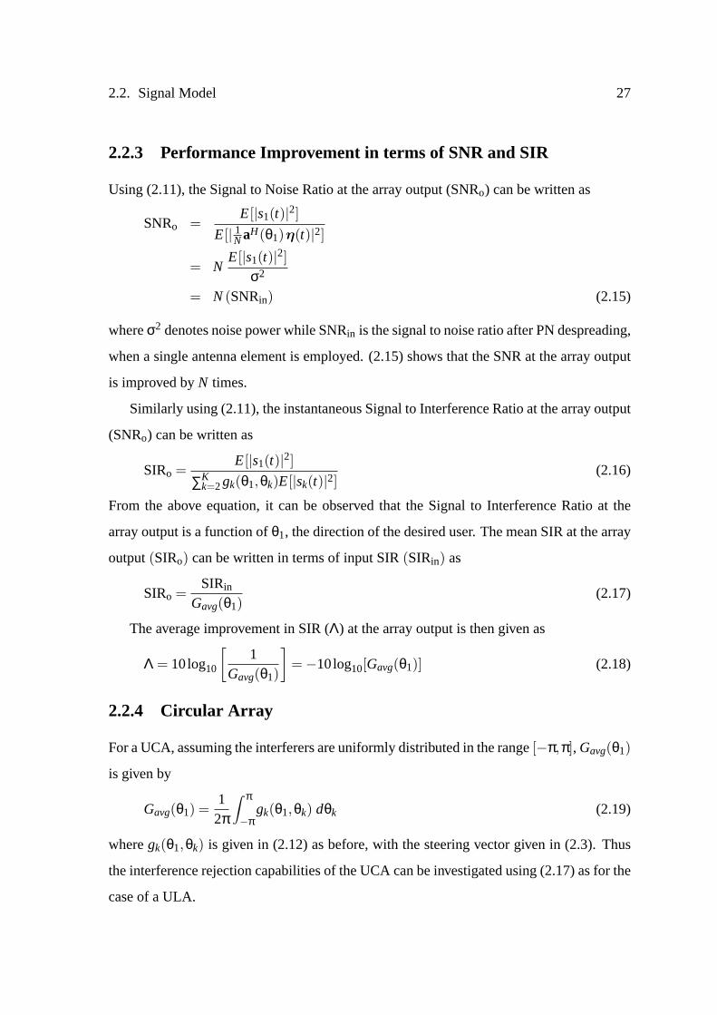
2.2. Signal Model 27
2.2.3 Performance Improvement in terms of SNR and SIR
Using (2.11), the Signal to Noise Ratio at the array output (SNRo) can be written as
SNRo =E[|s1(t)|2]
E[| 1NaH(θ1)η(t)|2]
= NE[|s1(t)|2]
σ2
= N(SNRin) (2.15)
whereσ2 denotes noise power while SNRin is the signal to noise ratio after PN despreading,
when a single antenna element is employed. (2.15) shows that the SNR at the array output
is improved byN times.
Similarly using (2.11), the instantaneous Signal to Interference Ratio at the array output
(SNRo) can be written as
SIRo =E[|s1(t)|2]
∑Kk=2gk(θ1,θk)E[|sk(t)|2]
(2.16)
From the above equation, it can be observed that the Signal to Interference Ratio at the
array output is a function ofθ1, the direction of the desired user. The mean SIR at the array
output(SIRo) can be written in terms of input SIR(SIRin) as
SIRo =SIRin
Gavg(θ1)(2.17)
The average improvement in SIR (Λ) at the array output is then given as
Λ = 10log10
[1
Gavg(θ1)
]=−10log10[Gavg(θ1)] (2.18)
2.2.4 Circular Array
For a UCA, assuming the interferers are uniformly distributed in the range[−π,π], Gavg(θ1)
is given by
Gavg(θ1) =12π
∫ π
−πgk(θ1,θk) dθk (2.19)
wheregk(θ1,θk) is given in (2.12) as before, with the steering vector given in (2.3). Thus
the interference rejection capabilities of the UCA can be investigated using (2.17) as for the
case of a ULA.

28 Chapter 2. Interference Rejection Capabilities of Array Antennas
2.3 Mutual Coupling
Thus far in this chapter, it has been assumed that the elements of the array antenna are
independent isotropic point sensors that sample but do not reradiate the incident signal.
However in a real system, each antenna element has some physical size and the elements
sample and reradiate the incident signal. The reradiated signals interact with the surround-
ing elements causing the elements to be mutually coupled. Mutual coupling is the name
given to this phenomenon that a current flowing in one antenna element can induce a volt-
age on a neighbouring antenna element.
To model the effects of mutual coupling, a mutual impedance matrix is used to char-
acterize the interaction among the array antenna components [130]. Mathematically, the
mutual impedance matrixZ is given by
Z =
ZA Z12 . . . Z1n
Z21 ZA . . . Z2n...
......
...Zn1 Zn2 . . . ZA
(2.20)
whereZA is the element’s impedance in isolation (forλ/2 dipole, its value isZA = 73+
j42.5 ohm), ZT is the impedance of the receiver at each element and is chosen as the
complex conjugate ofZA to obtain an impedance match for maximum power transfer.
In general, numerical techniques such as Method of Moments [131] or Full-Wave Elec-
tromagnetic Numerical Computation [132] can be used to obtain the mutual impedance
matrix. For dipoles, however,Z can be easily determined using classical Induced Electro-
motive Force (EMF) method [32].
2.3.1 Induced EMF Method
Induced EMF method is a classical method of computing the self and mutual impedances
of an antenna array. This method is restricted to straight and parallel elements in formation
and does not account for the radii of the wires and the gaps at the feeds. However, the
advantage of this method is that it leads to closed form solutions for the three classic cases
of side-by-side, collinear and parallel-in-echelon configurations [36].

2.3. Mutual Coupling 29
For the side-by-side configuration and dipole lengthsl = λ/2, an element of the mutual
impedance matrixZmn, where 1≤m,n≤ N, is given by [32]
Zmn =
30[0.5772+ ln(2K l)−Ci(2K l)]+
j[30Si(2K l)], m= n (2.21a)
30[2Ci(u0)−Ci(u1)−Ci(u2)]−
j[30(2Si(u0)−Si(u1)−Si(u2))], m 6= n (2.21b)
whereK is the wave number,dh is the horizontal distance between the two dipole antennas
and
u0 = K dh (2.22)
u1 = K (√
d2h + l2 + l) (2.23)
u2 = K (√
d2h + l2− l) (2.24)
andCi(u) andSi(u) are the Cosine and Sine integrals respectively, defined as [133]
Ci(u) =∫ u
∞
cos(x)x
dx (2.25)
Si(u) =∫ u
0
sin(x)x
dx (2.26)
2.3.2 Modified Signal Model
In order to include effect of mutual coupling for both linear and circular arrays, a mutual
coupling matrix is inserted in the model for the received signal, modifying (2.5) to
x(t) =K
∑k=1
C a(θk)sk(t)+η(t) =K
∑k=1
aMC(θk)sk(t)+η(t) (2.27)
whereaMC(θk) = C a(θk) is the modified array steering vector andC is the coupling matrix
of the antenna array, which can be written using fundamental electromagnetics and circuit
theory as [134]
C = (ZA +ZT)(Z +ZT IN)−1 (2.28)
whereIN is theN×N identity matrix andZ is the mutual impedance matrix in (2.21).

30 Chapter 2. Interference Rejection Capabilities of Array Antennas
In addition, the beamforming weight vector is modified as
wMC =1N
C a(θ1) (2.29)
Once theC matrix has been obtained, the capability of the array including mutual cou-
pling effects can be assessed by finding the mean output power of the processor, as before,
and identifying the signal, noise and interference power terms respectively. Repeating the
analysis in the last section, it can be shown that with mutual coupling matrix taken into
account the normalized amount of interference power seen from an interfererk at angle of
arrival θk is
gk(θ1,θk) =∣∣∣∣ wH
MC aMC(θk)||wH
MC|| ||aMC(θk)||
∣∣∣∣2 (2.30)
wherewMC is given in (2.29) andaMC(θk) in (2.27) respectively. The numerator in (2.30)
after substituting the values becomes∣∣wHMC aMC(θk)
∣∣2 =∣∣∣∣[ 1
NC a(θ1)]H [C a(θk)]
∣∣∣∣2=
1N2
∣∣aH(θ1) CH C a(θk)∣∣2 (2.31)
(2.30) is then substituted in (2.14) and (2.19) to get the spatial interference suppression
coefficient for linear and circular arrays respectively.
2.4 Results
2.4.1 Mutual Impedance Matrix
When there is no mutual coupling, the matrixZ appearing in (2.20) is diagonal. In the
presence of mutual coupling between antenna elements, there are non-zero elements off the
diagonal. Figure 2.3 shows the plot of the magnitude of the normalized impedance matrix
elements for an array ofN = 12, l = λ/2 dipoles with terminating impedanceZT = ZA for
(a) linear and (b) circular geometries respectively. The figure shows that for a linear array,
the coupling between the neighbouring elements is almost the same along the array. Also
the magnitude of the coupling decreases quite rapidly as we move away from the diagonal.
For a circular array, the magnitude also decreases initially but it increases again due to the
circular symmetry of the geometry.
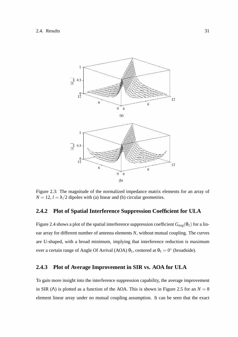
2.4. Results 31
Figure 2.3: The magnitude of the normalized impedance matrix elements for an array ofN = 12, l = λ/2 dipoles with (a) linear and (b) circular geometries.
2.4.2 Plot of Spatial Interference Suppression Coefficient for ULA
Figure 2.4 shows a plot of the spatial interference suppression coefficientGavg(θ1) for a lin-
ear array for different number of antenna elementsN, without mutual coupling. The curves
are U-shaped, with a broad minimum, implying that interference reduction is maximum
over a certain range of Angle Of Arrival (AOA)θ1, centered atθ1 = 0 (broadside).
2.4.3 Plot of Average Improvement in SIR vs. AOA for ULA
To gain more insight into the interference suppression capability, the average improvement
in SIR (Λ) is plotted as a function of the AOA. This is shown in Figure 2.5 for anN = 8
element linear array under no mutual coupling assumption. It can be seen that the exact

32 Chapter 2. Interference Rejection Capabilities of Array Antennas
−90 −60 −30 0 30 60 900
0.05
0.1
0.15
0.2
0.25
0.3
0.35
0.4
0.45
AOA θ1 (degrees)
Gav
g(θ1)
N = 4N = 8N = 12N = 16N = 20
N = 4
N = 8
Figure 2.4: Variation of the spatial interference coefficientGavg(θ1) with AOA θ1 for ULAantenna(N = 4,8,12,16,20), without mutual coupling.
amount of SIR at the array output is dependent on AOAθ1. The maximum SIR improve-
ment of about 10.85 dB is achieved when DOA isθ = 0. However this decreases by more
than half to about 5.1 dB for end-fire incidence. The presented result confirms the expecta-
tion that for a linear array its discrimination against interferers (in terms of SIR) is best in
the array’s broadside direction and deteriorates in its end-fire directions.
2.4.4 Interference Reduction Beamwidth
To characterise this degradation in performance as we move from broadside to end-fire
direction, we can define an ‘Interference Reduction Beamwidth’(BWir ) as the range of
AOA θ1 over whichGavg(θ1) is within 3 dB of its maximum value at 0. Figure 2.6 shows
the variation ofBWir with N. ForN = 4, the beamwidth is approximately±51 but increases
to about±59 for N = 12. The range is nearly the same whenN increases further, with a
small oscillation about this value, implying the onset of diminishing returns.

2.4. Results 33
0 15 30 45 60 75 900
2
4
6
8
10
12A
vera
ge im
prov
emen
t in
SIR
Λ (d
B)
AOA θ1 (degrees)
3 dB
Interference Reduction Beamwidth
Figure 2.5: Plot of Average Improvement in SIR versus AOAθ1 for N = 8 ULA antenna,under no mutual coupling assumption.
4 8 12 16 20 24 2845
50
55
60
65
BW
ir(D
egre
es)
Number of antenna elements N
Figure 2.6: Plot of ‘Interference Reduction Beamwidth’ versus number of antenna elementsN, for a ULA antenna under no mutual coupling assumption.

34 Chapter 2. Interference Rejection Capabilities of Array Antennas
2.4.5 Effect of Mutual Coupling on Spatial Interference SuppressionCoefficient for ULA
Figure 2.7 shows a plot of the spatial interference suppression coefficientGavg(θ1) for a
linear array for different number of antenna elementsN with mutual coupling. TheZ matrix
is obtained using the Induced EMF method. The figure shows that for a linear array, mutual
coupling degrades the SIR improvement capability of the array. For larger scan angles, the
performance is the same as for the case of no mutual coupling, but for broad-side incidence
there is degradation due to mutual coupling.
2.4.6 Plot of Spatial Interference Suppression Coefficient for UCA
The plot ofGavg(θ1) for circular array is shown in Figure 2.8. For a smaller number of
antenna elements, the SIR improvement shows an oscillatory variation. However asN
increases the curves flatten, indicating uniform SIR improvement over all angles.
For the case when mutual coupling is considered, theZ matrix is obtained using Induced
EMF method and also using FEKO [39], which is a commercially available electromagnetic
analysis package based on the Method of Moments (in FEKO simulations, frequency of 2
GHz and a wire radius of 0.5mm or 3.33×10⁻³λ are assumed). From the figure, it can be
observed that contrary to the case of the linear array, a slight improvement in performance
can be observed when mutual coupling is included, for all scan angles. The figure also
shows that the curves obtained usingZ determined from the Induced EMF method show
a good agreement with the curves obtained usingZ calculated from FEKO. The slight
difference in the curves can be attributed to limitations of the Induced EMF method, e.g. it
cannot take into account the gaps at the feed and the radius of the wires.
2.4.7 Variation of Mean of Spatial Interference Suppression Coeffi-cient with N
Finally, Table 2.1 shows a comparison of mean ofGavg(θ1) over AOA θ1 for different
N for linear and circular arrays, with and without mutual coupling. The mean is taken
over 180 (−π/2≤ θ ≤ π/2) for linear array and 360 (−π ≤ θ ≤ π) for circular array.

2.4. Results 35
−90 −60 −30 0 30 60 900
0.05
0.1
0.15
0.2
0.25
0.3
0.35
0.4
0.45
0.5
AOA θ1 (degrees)
Gav
g(θ1)
without mutual couplingwith mutual coupling(Induced EMF)
N = 4
N = 12
N = 8
Figure 2.7: Variation of the spatial interference coefficientGavg(θ1) with AOA θ1 for ULAantenna(N = 4,8,12), with and without mutual coupling.
−180 −120 −60 0 60 120 1800
0.05
0.1
0.15
0.2
0.25
0.3
0.35
0.4
AOA θ1 (degrees)
Gav
g(θ1)
without mutual couplingwith mutual coupling (Induced EMF)with mutual coupling (FEKO)
N = 4
N = 8
N = 12
Figure 2.8: Variation of the spatial interference suppression coefficientGavg(θ1) with AOAθ1 for UCA antenna(N = 4,8,12), with and without mutual coupling.

36 Chapter 2. Interference Rejection Capabilities of Array Antennas
Table 2.1: Mean ofGavg(θ1) over AOA θ1 for linear and circular arrays, with and withoutmutual coupling
N
Mean ofGavg(θ1) over AOA θ1
Linear Circular
without coupling with coupling without coupling with coupling
4 0.3021 0.3667 0.3241 0.2926
8 0.1668 0.2369 0.1683 0.1438
12 0.1176 0.1852 0.1134 0.0996
16 0.0917 0.1558 0.0915 0.0811
20 0.0756 0.1363 0.0774 0.0722
The table shows that when averaged over all values of AOA, both arrays show a similar
performance for the case of no mutual coupling. This conclusion is in good agreement
with the findings recently reported in [135]. However when mutual coupling is taken into
account, the values are higher for a linear array indicating a degradation in performance
while for a circular array the values are slightly reduced indicating a small improvement in
performance. The values also confirm that for largeN, the interference rejection capability
reaches an asymptotic level both with or without mutual coupling.
2.5 Summary
This chapter has addressed the modelling of linear and circular array of half-wavelength
spaced dipoles, which can be part of a base station of a CDMA cellular communication
system. The performance of these two array antennas has been compared in terms of their
interference rejection capabilities for the two cases of with and without mutual coupling. It
has been shown that a circular array provides a more uniform improvement in terms of SIR
than a linear array and is less susceptible to the effects of mutual coupling. However when
the performance is averaged over all angles of arrival and mutual coupling is negligible,
linear arrays show similar performance to circular arrays. Thus in the remaining chapters
of this thesis, only linear arrays are considered.

Chapter 3
Description and Modelling of WirelessChannel
In this chapter a new spatio-temporal channel model, for use in the performance analysis of
wireless communication systems incorporating smart antennas, is presented. As mentioned
in Chapter 1, there are several ways to characterize the wireless propagation environment.
This chapter describes the construction of a parameterized physical channel model for smart
antennas and is organised as follows. In Section 3.1, modelling of the various spatial and
temporal parameters of the channel model is described. In Section 3.2, these parameters are
then combined into a single channel model and a mathematical description of the model is
presented. Finally, the proposed model is implemented in software and Sections 3.3 and 3.4
present and discuss different Rayleigh and Rician fading channel simulations respectively.
3.1 Physical Channel Model Parameters
Consider the scenario where the Base Station (BS) is an elevated and separate structure that
is located well above the surrounding scatterers. Without loss of generality, it is assumed
that the BS employs a Uniform Linear Array (ULA) ofN omni-directional antenna ele-
ments, with inter-element spacingd = λ/2. The Mobile Station (MS), however, moves on
the street level (at a typical height of 1−2 m) and is surrounded by local scattering struc-
tures (e.g., an urban or suburban environment). Furthermore, a few dominant and spatially
well-separated reflectors, such as hills or large buildings, are located in the environment in
the far-field of the array. The propagation scenario is illustrated in Figure 3.1.
37

38 Chapter 3. Description and Modelling of Wireless Channel
Local scatteringstructuresaround the MS
y
Dominant reflector
Subpaths
MeanAOA θk
N element ULAantenna at BS
x
Angular dispersion ofreceived signal at theBS, characterized byangle spread σAOA
Figure 3.1: Illustration of wireless propagation environment.
The signal transmitted by the MS illuminates the local scattering structures around the
MS. This generates numerous subpaths of the signal. The subpaths reach the BS either
directly (line-of-sight propagation) or after undergoing further reflection from a dominant
reflector (non-line-of-sight propagation), which gives rise to multipath propagation. Each
propagation path arriving at the BS is itself composed of a large number of subpaths, which
cannot be resolved by the receiver because their relative time delay is too small (i.e. less
than one chip duration). Since the dominant reflectors are significantly separated, a different
combination of the incoming subpaths is reflected at each reflector. Therefore independent
fading is assumed for each path. In case of movement of the MS, the superposition of the
subpaths results in time-correlated multipath fading.
Each propagation path is associated with its own power, time delay and angle of arrival.
In general, the received signal at the BS arrives mainly from one given direction. In addi-
tion, a small angle spread of subpaths is observed at the BS as the MS is far away from the
BS and the BS is well above the surrounding objects.
Various parameters of the physical model, that are used to characterise the wireless

3.1. Physical Channel Model Parameters 39
channel between the MS and BS, can be grouped into the following two main categories:-
1. Temporal Parameters
(a) Path loss.
(b) Shadowing.
(c) Multipath fading.
(d) Power Spectral Density.
(e) Power Delay Profile.
2. Spatial Parameters
(a) Angle of Arrival.
(b) Angular distribution of users.
(c) pdf’s in Angles of Departure and Angles of Arrival.
(d) Spatial correlation.
(e) MS mobility.
The modelling of these parameters is detailed in the following subsections.
3.1.1 Path Loss
Path loss is defined as an overall decrease in signal strength with distance between the
transmitter and receiver [136]. Measurements show that the average received signal power
decreases logarithmically with distance [2]. The average path lossρ(Dk) can thus be ex-
pressed as
ρ(Dk) = ρ(D0)+10ε log10
(Dk
D0
), dB (3.1)
whereε is the path loss exponent that indicates the rate of signal power attenuation with
distance,D0 is the close-in reference distance which is determined from measurements
close to the transmitter,Dk is the distance between thekth MS and the BS andρ(D0) is
the average path loss at close-in reference distance [2]. The value ofε depends on the
specific propagation environment, e.g. in free spaceε = 2. For a typical urban macrocell
environment, the value ofε ranges between 2 and 5, with a typical value of 4 [2].

40 Chapter 3. Description and Modelling of Wireless Channel
3.1.2 Shadowing
Shadowing or slow fading represents the variation of average path loss in a local area (sev-
eral tens of meters). It is caused by variation of propagation conditions due to buildings,
roads, trees and other obstacles in a relatively small area [137].
Empirical studies show that the received signal levels at a specific transmitter-receiver
separation have a Gaussian distribution about the distance dependent average path loss
from (3.1), where the measured signal levels have values in dB units [2]. Thus considering
shadowing, the overall path lossρ(Dk) is given by
ρ(Dk) = ρ(Dk)+Sk, dB (3.2)
whereρ(Dk) is given in (3.1) andSk is a zero mean Gaussian distributed random variable
(in dB) with varianceσ2S (also in dB). The variance usually lies in the range 4− 12 dB,
depending upon the propagation environment. For urban macrocells, typical value forσ2S
is 8 dB [107].
Shadowing and path loss both affect the mean power of the received signal and their
combined effect changes slowly over time due to motion of the MS. It is assumed that
these slow-fading effects are compensated for by the perfect power control system and are
therefore not considered in the simulations.
3.1.3 Multipath Fading
When a radio signal is transmitted in a wireless channel, the waves propagate through the
physical medium (atmosphere or free space) and interact with the physical objects that
constitute the propagation environment such as buildings, hills, trees and moving vehi-
cles, giving rise to many subpaths of the transmitted signal. Multipath fading is caused
by the constructive and destructive combination of these randomly delayed, reflected, scat-
tered and diffracted subpath signal components over distances of the order of a few wave-
lengths [42]. This type of fading is relatively fast and is therefore responsible for short-term
signal variations.

3.1. Physical Channel Model Parameters 41
Depending on the nature of the propagation environment, the multipath fading envelope
can be described by different models [42]. In this thesis the Rayleigh (non-line-of-sight)
and Rician (line-of-sight) fading models, which are most commonly used to describe the
statistical time varying nature of the individual multipath envelopes, are considered [2].
3.1.3.1 Rayleigh Model
The Rayleigh distribution can be used to model the multipath fading in Non-Line-Of-Sight
(NLOS) fading environments, i.e. when there is no direct Line-Of-Sight (LOS) path be-
tween the MS and BS. In this case, the channel fading amplitudeα is distributed according
to
fα(α) =2αΩ
exp
(−α2
Ω
), α≥ 0 (3.3)
whereΩ = E[α2] is the average envelope power andE[·] denotes expectation operator.
3.1.3.2 Rice Model
The Rice distribution is used to model the propagation paths consisting of one direct LOS
component and many random weaker NLOS components. In this case, the channel fading
amplitude is distributed according to [107]
fα(α) =2αb0
exp
(−α2 +s2
2b0
)I0
(αsb0
), α≥ 0 (3.4)
wheres2 is the specular power, 2b0 is the scattered power andI0(·) is the modified Bessel
function of the first kind and zero order [133].
The Rice factorKR is defined as the ratio of the specular power to the diffuse or scattered
power. This ratio is commonly expressed in decibels as
KR = 10log10
(s2
2b0
)(3.5)
The Rice factor completely specifies the Rice distribution. In terms of the Rice factor,
the specular and scattered powers can be written as [107]
s2 =KRΩ
KR+1(3.6a)
2b0 =Ω
KR+1(3.6b)

42 Chapter 3. Description and Modelling of Wireless Channel
0 0.5 1 1.5 2 2.5 30
0.5
1
1.5
2
2.5
3
α
f α(α)
KR = −∞ dB
KR = 1 dB
KR = 5 dB
KR = 10 dB
Figure 3.2: The Rice probability density function for Rice factorsKR = −∞,1,5,10 dBrespectively.
whereΩ = s2+2b0 is the average envelope power. Using (3.6a) and (3.6b), the probability
density function (pdf) of the Rice distribution can be written as [138]
fα(α) =2α(KR+1)
Ωexp
(−KR−
(KR+1)α2
Ω
)I0
(2α√
KR(KR+1)Ω
), α≥ 0 (3.7)
Figure 3.2 shows the Rice pdf for several values ofKR. The curve forKR = −∞ dB
corresponds to the Rayleigh pdf. It can be seen that the Rician pdf degenerates to a Rayleigh
pdf as the value ofKR→−∞ dB.
3.1.4 Power Spectral Density
Whenever relative motion exists between the transmitter and receiver, it causes an appar-
ent shift in the frequency of the received signal due to the Doppler shift. The Doppler
shift is different for every subpath as it depends on the Angle of Departure (AOD) of the
subpath relative to the direction of movement of the MS. For the sum of all the scattered

3.1. Physical Channel Model Parameters 43
and reflected subpaths, this yields a continuous spectrum of Doppler frequencies, called the
Power Spectral Density (PSD). The inverse Fourier transform of the PSD is the autocorre-
lation function of the fading signal [107,139].
The shape of the PSD determines the time domain fading signal and its temporal corre-
lation properties. The proper selection of the fading spectrum is, therefore, very important
in order to produce realistic fading signals that have proper temporal correlation behaviour.
Depending upon the particular propagation environment and the underlying communica-
tion scenario, different PSD’s have been proposed [42]. A popular choice for land mobile
communications, which is also adopted this thesis, is the Jakes PSD [45,46].
For the case of Rayleigh fading, the normalised Jakes PSD and the corresponding auto-
correlation function are given by [42]
S( f ) =1
π fD√
(1− ( f/ fD)2, | f | ≤ fD (3.8a)
R(τ) = J0(2π fD τ) (3.8b)
whereJ0(·) is the zero-order Bessel function of the first kind andfD is the maximum
Doppler shift that the signal undergoes, given by
fD =vλ
=v fcc
(3.9)
wherev is the vehicle speed (in m/s),λ is the wavelength of the transmitted signal,c is the
velocity of light andfc is the carrier frequency.
In this thesis, the maximum Doppler frequency used is 100 Hz. This corresponds to a
speed ofv = 120 km/hr for fc = 900 MHz andv = 54 km/hr for fc = 2 GHz respectively
(i.e. a fast vehicular channel). Figure 3.3 shows a plot of the autocorrelation function
against the time delay assumingfD = 100 Hz.
3.1.5 Power Delay Profile
The information about the multipath delays (τl ) and powers (Ωl = E[(αl )2]) is conveniently
represented using the channel’s Power Delay Profile (PDP), which is also referred to as the
Multipath Intensity Profile (MIP). It shows the mean power present at different time delays.

44 Chapter 3. Description and Modelling of Wireless Channel
0 10 20 30 40 50−0.6
−0.4
−0.2
0
0.2
0.4
0.6
0.8
1
Time delay τ (ms)
Aut
ocor
rela
tion
func
tion
R (τ
)
fD
= 100 Hz (Rayleigh)
Figure 3.3: The autocorrelation function corresponding to the Jakes power spectral densityfor fD = 100 Hz.
The PDP model can assume various forms, depending on the type of environment (indoor
or outdoor) and the general propagation conditions [140]. In this work, the simplifying
assumption is made that the time delays associated with the different resolvable multipaths
are independent of the Angles of Arrival (AOA’s) [71].
An important measure which characterizes the time dispersiveness of the channel is the
RMS delay spreadσDS. It is defined as the square root of the second central moment of the
PDP and is given as [2]
σDS =√
τ2− (τ)2 (3.10)
where
τ2 =∑l
Ωl (τl )2
∑l
Ωl(3.11)
and τ is the first moment of the power delay profile called the mean excess delay. It is

3.1. Physical Channel Model Parameters 45
Table 3.1: Typical RMS delay spread values reported in literature [141].
Environment RMS Delay Spread (µs)
Suburban 0.1−1
Urban 1−3
Rural 6−7
defined as [2]
τ =∑l
Ωl τl
∑l
Ωl(3.12)
(3.11) and (3.12) do not rely on the absolute path powers but only on the relative am-
plitudes. The delays in the above equations are measured relative to the first path. Typ-
ical values for the RMS delay spread at 900 MHz reported in literature are shown in Ta-
ble 3.1 [141].
In this thesis, a uniform PDP is assumed. The two-path model is often used for analyti-
cal treatments. The impulse response for this model can be written as [142]
h(t) = α1δ(t− τ1)+α2δ(t− τ2) (3.13)
whereτ1 andτ2 are the path delays andα1 andα2 are the complex fading coefficients. The
PDP can be written as
P(τ) = Ω1δ(t− τ1)+Ω2δ(t− τ2) (3.14)
whereΩ1 andΩ2 are the path powers respectively.
The two- and and three-path PDP’s used in the work are shown in Figure 3.4 [2].
3.1.6 Mean Angle of Arrival
Each MS’s incoming signal at the BS is described with a mean Angle of Arrival (AOA)θk.
It is assumed that the AOA is the same for all the multipaths of a particular user, i.e. the
spatial channel is assumed to be based on one AOA only (θk,l = θk). As per convention, the
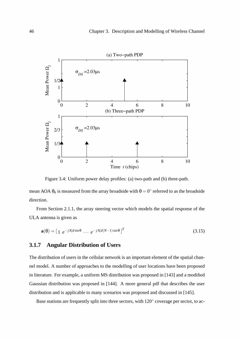
46 Chapter 3. Description and Modelling of Wireless Channel
0 2 4 6 8 100
11/2
1
Mea
n Po
wer
Ωl
(a) Two−path PDP
σDS
=2.03µs
0 2 4 6 8 100
1/3
2/3
1
Time t (chips)
σDS
=2.03µs
(b) Three−path PDP
Mea
n Po
wer
Ωl
Figure 3.4: Uniform power delay profiles: (a) two-path and (b) three-path.
mean AOAθk is measured from the array broadside withθ = 0 referred to as the broadside
direction.
From Section 2.1.1, the array steering vector which models the spatial response of the
ULA antenna is given as
a(θ) = [ 1 e− jK dsinθ · · · e− jK d(N−1)sinθ ]T (3.15)
3.1.7 Angular Distribution of Users
The distribution of users in the cellular network is an important element of the spatial chan-
nel model. A number of approaches to the modelling of user locations have been proposed
in literature. For example, a uniform MS distribution was proposed in [143] and a modified
Gaussian distribution was proposed in [144]. A more general pdf that describes the user
distribution and is applicable to many scenarios was proposed and discussed in [145].
Base stations are frequently split into three sectors, with 120 coverage per sector, to ac-

3.1. Physical Channel Model Parameters 47
commodate more users per base station. In this thesis, a single 120 sector is considered for
compatibility with the tri-sectored approach used by most of the current commercial sys-
tems. It is assumed that theK users in the system are uniformly distributed in[−60, 60],
along the arc boundary of the sector cell in the far field of the array.
3.1.8 Azimuth Field Dispersion at MS and BS
One of the most important spatial assumption relates to the probability density function
(pdf) of the Angle of Departure (AOD) of the subpaths at the MS and the pdf of the Angle
of Arrival (AOA) of the subpaths at the BS respectively. There is a fundamental difference
between azimuthal field dispersion at an elevated BS and a MS, even though the propaga-
tion channel is assumed to be reciprocal, e.g at the elevated BS, the incoming field can be
expected to be more concentrated in azimuth since the BS antenna is located well above the
scatterers [57].
3.1.8.1 pdf in AOD
The pdf in the AOD at the MS describes the angular distribution of the subpaths departing
the MS in azimuth. It is assumed that the azimuth field distribution at the MS can be
modelled by a uniform probability density function over[0,2π]. This corresponds to the
isotropic scattering model, also known as the Clarke’s model [45,46]. Recently, it has been
suggested that von Mises distribution provides a more accurate description of the angular
distribution of the subpaths at the MS [146,147].
3.1.8.2 pdf in AOA
The pdf in the AOA at the BS describes the angular distribution of the subpaths arriving
at the BS in azimuth. For urban environments, a commonly used assumption for azimuth
energy distribution is a uniform distribution [148], given by
fAOA(θ) =1
2∆, θk−∆≤ θ≤ θk +∆ (3.16)
where∆ is called the scattering angle and is related to the standard deviation of the uniform
distribution asσAOA = ∆√3
and 2∆ is the range of angles about the Mean AOAθk.

48 Chapter 3. Description and Modelling of Wireless Channel
Another distribution that has been suggested is a Gaussian distribution in AOA, given
by [149]
fAOA(θ) =Cg√
2πσAOAexp
[(θ−θk)2
2σ2AOA
], −π+θk ≤ θ≤ π+θk (3.17)
whereσAOA is the standard deviation and controls the spread of the pdf function andCg is a
constant that ensures thatfAOA(θ) fulfils the requirements of a pdf, given by [150]
Cg =1
erf(π/√
2σAOA)(3.18)
where erf(x) = 2/(√
π)∫ x
0 e−t2dt is the error function. Note that when angular spread is
small,Cg is almost unity. The uniform and Gaussian distributions are shown in Figures 3.5
and 3.6 respectively for various angle spreadsσAOA= 5,10,20,60 about the mean AOA
θ = 0.
In addition to the uniform and Gaussian distributions, other distributions have also been
proposed, e.g. cosn(θ) [62] and Laplacian distributions [151, 152]. According to [57],
a Gaussian pdf best matches the azimuth pdf in typical urban environments. However
from the point of view of simulations, the key parameter of the system performance is the
standard deviation of the pdf in AOA and not the type of pdf in AOA under investiga-
tion [115,153,154].
3.1.9 Spatial Correlation Coefficient
The performance of different antenna array architectures is dependant on the spatial corre-
lation between the antenna elements, e.g. traditional beamforming techniques depend on
the perfect correlation of the received signals at the array while diversity techniques depend
on low correlation of the received signal between the antenna branches. Thus it is important
to study the cross-correlation behaviour for different environment conditions. The cross-
correlation between the waves impinging on two antenna elements depends mostly on the
pdf in AOA. In this section, both uniform and Gaussian distributions are employed to model
the AOA’s and their impact on array spatial correlation is considered. To allow a consistent
comparison, the Angle Spread (AS) is assumed equal to the standard deviationσAOA of the
underlying pdf.

3.1. Physical Channel Model Parameters 49
−3 −2 −1 0 1 2 30
0.5
1
1.5
2
2.5
3
3.5
4
AOA θ (radians)
f AO
A(θ)
σAOA
= 5°σ
AOA = 10°
σAOA
= 20°σ
AOA = 60°
Figure 3.5: Uniform pdf’s in azimuth AOA for mean AOAθ = 0 and angle spreadsσAOA=5,10,20,60 respectively.
−3 −2 −1 0 1 2 30
0.5
1
1.5
2
2.5
3
3.5
4
4.5
5
AOA θ (radians)
f AO
A(θ)
σAOA
= 5°σ
AOA = 10°
σAOA
= 20°σ
AOA = 60°
Figure 3.6: Gaussian pdf’s in azimuth AOA for mean AOAθ = 0 and angle spreadsσAOA=5,10,20,60 respectively.

50 Chapter 3. Description and Modelling of Wireless Channel
The array spatial correlation between thenth andpth antenna elements for the ULA is
defined as
Rs(n, p) = Ean(θ)a∗p(θ)
=∫
θan(θ)a∗p(θ) fAOA(θ)≡ℜRs(n, p)+ jℑRs(n, p) (3.19)
where(·)∗ denotes complex conjugate,fAOA(θ) is the pdf of the AOA distribution andan(θ)
andap(θ) are elements of the array steering vector from (3.15).
The spatial envelope correlation coefficientρs is then defined as
ρs = |Rs(n, p)|2 = |ℜRs(n, p)+ jℑRs(n, p)|2 (3.20)
whereℜRs(n, p) andℑRs(n, p) are the real and imaginary parts of signal correlation
respectively. The required antenna separation forρs = 0.7 is also known as the correlation
distance.
Assuming a uniform distribution in AOA, the real and imaginary parts of signal corre-
lation between thenth andpth antenna elements are given by [148,155]
ℜRs(n, p) = J0(znp)+2∞
∑v=1
J2v(znp) cos(2vθ) sinc(2v∆) (3.21a)
ℑRs(n, p) = 2∞
∑v=0
J2v+1(znp) sin[(2v+1)θ]sinc[(2v+1)∆] (3.21b)
whereznp = 2π|p− n|d/λ, d is the inter-element distance,λ is the wavelength,θ is the
mean AOA,∆ is the scattering angle,Jn(x) is thenth order Bessel function of the first kind
and sinc(x) = sin(x)x is the sinc(·) function.
Assuming a Gaussian distribution in AOA, it can be shown that the real and imaginary
parts ofRs(n, p) are given by [149,156]
ℜRs(n, p) = J0(znp)+2Cg
∞
∑v=1
J2v(znp) cos(2vθ)
exp(−2v2σ2
AOA
)ℜ
erf
(π+ j2vσ2
AOA√2σAOA
)(3.22a)
ℑRs(n, p) = 2Cg
∞
∑v=0
J2v+1(znp)sin[(2v+1)θ]
exp
[−(2v+1)2σ2
AOA
2
]ℜ
erf
[π+ j(2v+1)σ2
AOA√2σAOA
](3.22b)

3.1. Physical Channel Model Parameters 51
whereCg is given in (3.18) and erf(a+ jb) is the complex input error function [157].
(3.21) and (3.22) can be numerically evaluated using MATLAB [126]. For the numer-
ical evaluation, the summation of over 30 terms is enough for accuracy of six digits after
the decimal point [150]. Figures 3.7 and 3.8 show the plots ofρs assuming uniform and
Gaussian AOA’s and different angle spreads respectively. The figures show that in general,
the spatial correlation decreases with increasing angular spread, increasing inter-element
distance and decreasing angle of arrival as measured from the array broadside. The largest
correlation is achieved atθ = 90 andσAOA = 0. The consequences of this correlation
behaviour are two-fold [149]:-
• If the azimuth angular spread is small, the output signals of the elements of the BS
antenna array are strongly correlated. Therefore the array antenna will provide beam-
forming gain only.
• If the azimuth angular spread is moderate or large, the output signals of the elements
of the BS antenna array are not strongly correlated. Therefore in this situation, the
array antenna can provide diversity gain from spatial fading in addition to the beam-
forming gain.
3.1.10 MS Mobility Model
Modelling of MS mobility is a crucial subject for the simulation of space-time channels.
The movement of the MS influences both the spatial and temporal channel characteristics.
Also for the case of adaptive beamforming, the smart antenna must track and steer its beam
towards the desired user. Therefore, the performance of a smart antenna cannot be realisti-
cally evaluated without simulating MS mobility.
For implementation efficiency, the following assumptions are used to model the effects
of MS mobility [67]:-
• The number of subpaths and the number of multipath components are kept constant
as the mobile moves for a particular Monte Carlo simulation run.
• The subpath parameters (angles of departures, random phases and angular spread)
are kept constant as the mobile moves.
• Only the mean AOAθk of the path is adjusted as the mobile moves.

52 Chapter 3. Description and Modelling of Wireless Channel
00.
51
1.5
22.
53
3.5
40
0.2
0.4
0.6
0.81
Nor
mal
ised
inte
r−el
emen
t dis
tanc
e d
/λ
Spatial Envelope Correlation Coefficient ρs
(a) M
ean
AO
A θ
= 0
°, un
ifor
m p
df in
AO
A
σ AO
A = 5
°σ A
OA =
10°
σ AO
A = 2
0°σ A
OA =
60°
00.
51
1.5
22.
53
3.5
40
0.2
0.4
0.6
0.81
Nor
mal
ised
inte
r−el
emen
t dis
tanc
e d
/λ
Spatial Envelope Correlation Coefficient ρs
(c) M
ean
AO
A θ
= 3
0°, u
nifo
rm p
df in
AO
A
σ AO
A = 5
°σ A
OA =
10°
σ AO
A = 2
0°σ A
OA =
60°
00.
51
1.5
22.
53
3.5
40
0.2
0.4
0.6
0.81
Nor
mal
ised
inte
r−el
emen
t dis
tanc
e d
/λ
Spatial Envelope Correlation Coefficient ρs
(b) M
ean
AO
A θ
= 0
°, G
auss
ian
pdf i
n A
OA
σ AO
A = 5
°σ A
OA =
10°
σ AO
A = 2
0°σ A
OA =
60°
00.
51
1.5
22.
53
3.5
40
0.2
0.4
0.6
0.81
Nor
mal
ised
inte
r−el
emen
t dis
tanc
e d
/λ
Spatial Envelope Correlation Coefficient ρs
(d) M
ean
AO
A θ
= 3
0°, G
auss
ian
pdf i
n A
OA
σ AO
A = 5
°σ A
OA =
10°
σ AO
A = 2
0°σ A
OA =
60°
Figure 3.7: Spatial envelope correlation coefficient for mean AOA’sθ = 0,30 and anglespreadsσAOA= 5,10,20,60 assuming uniform and Gaussian pdf’s in AOA respectively.

3.1. Physical Channel Model Parameters 53
00.
51
1.5
22.
53
3.5
40
0.2
0.4
0.6
0.81
Nor
mal
ised
inte
r−el
emen
t dis
tanc
e d
/λ
Spatial Envelope Correlation Coefficient ρs
(a) M
ean
AO
A θ
= 6
0°, u
nifo
rm p
df in
AO
A
σ AO
A = 5
°σ A
OA =
10°
σ AO
A = 2
0°σ A
OA =
60°
00.
51
1.5
22.
53
3.5
40
0.2
0.4
0.6
0.81
Nor
mal
ised
inte
r−el
emen
t dis
tanc
e d
/λ
Spatial Envelope Correlation Coefficient ρs
(c) M
ean
AO
A θ
= 9
0°, u
nifo
rm p
df in
AO
A
σ AO
A = 5
°σ A
OA =
10°
σ AO
A = 2
0°σ A
OA =
60°
00.
51
1.5
22.
53
3.5
40
0.2
0.4
0.6
0.81
Nor
mal
ised
inte
r−el
emen
t dis
tanc
e d
/λ
Spatial Envelope Correlation Coefficient ρs
(b) M
ean
AO
A θ
= 6
0°, G
auss
ian
pdf i
n A
OA
σ AO
A = 5
°σ A
OA =
10°
σ AO
A = 2
0°σ A
OA =
60°
00.
51
1.5
22.
53
3.5
40
0.2
0.4
0.6
0.81
Nor
mal
ised
inte
r−el
emen
t dis
tanc
e d
/λ
Spatial Envelope Correlation Coefficient ρs
(d) M
ean
AO
A θ
= 9
0°, G
auss
ian
pdf i
n A
OA
σ AO
A = 5
°σ A
OA =
10°
σ AO
A = 2
0°σ A
OA =
60°
Figure 3.8: Spatial envelope correlation coefficient for mean AOA’sθ = 60,90 and anglespreadsσAOA= 5,10,20,60 assuming uniform and Gaussian pdf’s in AOA respectively.

54 Chapter 3. Description and Modelling of Wireless Channel
In the simulations, the mean AOA of the desired user is varied from−60 to 60 with
step size∆θ = 0.01 per snapshot to cover the entire azimuth range. This value of the step
size is widely used in the simulation studies, for instance [34,37,158]. It corresponds to an
angular speed of 48 degree/s and provides a worst case scenario for a very fast moving MS
at a very close distance to the BS, e.g. an MS travelling at velocity 300 km/hr at only 100
m from the BS. By comparison, when an MS travels at velocity 120 km/hr at a distance of
0.5 km from the BS, this corresponds to an angular speed of only 3.82 degree/s.
It must be noted that effect of mobility (Doppler frequencyfD) on temporal fading
characteristics is already taken into account, as explained in Section 3.1.4.
3.2 Channel Response Vector
Following the approach of [71], the temporal and spatial parameters discussed in the previ-
ous section can be combined into a single model. As discussed in Section 3.1, it is assumed
that the BS is equipped with a ULA ofN receive antennas while each MS has a single
transmit antenna. The signal received at the BS for thekth user consists ofL time delayed
multipath replicas of the transmitted signal. The individual paths are defined by their pow-
ers, delays and angles of arrival. Each path is itself a superposition ofS subpaths. These
subpaths arrive at the base station from a random directionθ(s)k,l = θk +ϑ(s)
k,l , whereθk is the
mean AOA andϑ(s)k,l is a zero mean random angular deviation with standard deviationσAOA.
The following two cases of Rayleigh and Rician fading are considered:-
3.2.1 Rayleigh Fading
For the case of Rayleigh fading multipaths, the total multiplicative distortion of thel th
resolvable path of thekth user at thenth antenna can be given as [71,116]
hk,l ,n(t) =
√Ωk,l
S
S
∑s=1
exp[
j(φ(s)k,l +2π fD t cosΨ(s)
k,l )]
exp[− jK d(n−1)sin(θk +ϑ(s)
k,l )]
=S
∑s=1
α(s)k,l exp
[− jK d(n−1)sinθ(s)
k,l
](3.23)
whereα(s)k,l denotes the complex subpath amplitude,Ωk,l is the mean path power (allS

3.2. Channel Response Vector 55
subpaths associated with thel th multipath have identical powersΩk,l/S), K = 2π/λ is
the wave number,d is the inter-element distance,φ(s)k,l is random phase of each subpath
uniformly distributed over[0,2π] and Ψ(s)k,l is the AOD for each subpath relative to the
motion of the mobile and is also uniformly distributed over[0,2π].
In vector notation, the spatial signature or channel response vector associated with the
l th multipath of thekth user can be expressed by aN×1 vector as
hk,l (t) =
[S
∑s=1
α(s)k,l
S
∑s=1
α(s)k,l e
[− jK dsin(θk+ϑ(s)k,l )] · · ·
S
∑s=1
α(s)k,l e
[− jK d(N−1)sin(θk+ϑ(s)k,l )]
]T
(3.24)
The following two special subcases of no angle spread and small angle spread are
considered:-
3.2.1.1 No Angle Spread
This subcase is applicable for the case of rural or suburban environments. It is equivalent
to the point source or plane wave channel model, which is commonly used when AOA
estimation algorithms are used [73]. In this case,θ(s)k,l = θk and (3.23) can be simplified as
follows
hk,l ,n(t) =
(S
∑s=1
α(s)k,l
)[exp(− jK d(n−1)sinθk)]
= αk,l (t) exp[− jK d(n−1)sinθk] (3.25)
whereαk,l (t) denotes the complex Rayleigh fading coefficient given by
αk,l (t) =S
∑s=1
α(s)k,l =
√Ωk,l
S
S
∑s=1
exp[
j(φ(s)k,l +2π fDt cosΨ(s)
k,l )]
(3.26)
The channel vector associated with the signal transmitted by thekth user can thus be
written as
hk,l (t) = αk,l (t)a(θk) (3.27)
wherea(θk) is theN×1 array steering vector given by (3.15).

56 Chapter 3. Description and Modelling of Wireless Channel
3.2.1.2 Moderate Angle Spread
This subcase is applicable to suburban and urban environments with angle spread in the
range 5−15 [57]. For the case of small to moderate angle spread, a Taylor expansion
of (3.23) gives [95]
hk,l (t)≈ αk,l a(θk)+ αk,l d(θk) (3.28)
wherea(θk) is the array steering vector andd(θk) is the gradient of the array steering vector,
which for a linear array is given by
d(θk) =ddθ
a(θk)
=[
0 − jK dcosθk e− jK dsinθk · · · − jK d(N−1)cosθk e− jK d(N−1)sinθk]T
(3.29)
and the constantsαk,l andαk,l are given by
αk,l =S
∑s=1
α(s)k,l (3.30a)
αk,l =S
∑s=1
α(s)k,l ϑ(s)
k,l (3.30b)
(3.28) shows that for a particular AOA, the time variant channel vectorhk,l (t) can be
represented as a linear combination of two time-invariant vectorsa(θk) andd(θk) and two
uncorrelated time-variant weightsαk,l and αk,l . This fact can be used in estimating the
channel vector for smart antenna applications [95].
3.2.2 Rician Fading
For the case of Rician fading (L = 1), which is relevant to urban micro-cellular areas with
a direct LOS component, the channel impulse response for thekth user at thenth antenna
is given as [71,117]
hk,n(t) =√
KR
1+KRh(LOS)
k,n (t)+√
11+KR
h(NLOS)k,n (t) (3.31)

3.3. Rayleigh Fading Channel Simulations 57
whereKR is the Rician factor given in (3.5) andh(LOS)k,n (t) andh(NLOS)
k,n (t) are the specular
and scattered components given by
h(LOS)k,n (t) = exp
[j(φ(LOS)
k +2π fD t cosθk)]
exp[− jK d(n−1)sinθk] (3.32)
h(NLOS)k,n (t) =
1√S
S
∑s=1
exp[
j(φ(s)k +2π fD t cosΨ(s)
k )]
e[− jK d(n−1)sinθk] (3.33)
whereφ(LOS)k is the random phase of the LOS subpath. It can be observed thath(NLOS)
k,n (t) is
a random process whileh(LOS)k,n (t) is deterministic.
3.3 Rayleigh Fading Channel Simulations
The results in this section are obtained by implementing (3.23), using the simulation model
developed for the purpose (see Appendix B). The value ofS= 15 subpaths is used in the
simulations. The following cases are considered:-
3.3.1 Single Antenna, Zero Angle Spread
Figure 3.9 shows the magnitude (a) and phase (b) of the simulated channel response for
a total time period of 100 ms, assuming a Doppler frequencyfD = 100 Hz. The distance
covered by the mobile station during this time period is equal to 3.33 m or 10λ. It can be
seen that deep fades occur with a periodicity of almost half wavelength. Also the occurrence
of deep fades coincides with the rapid jumps in the phase plot.
Figure 3.9 (c) shows the probability density histogram of the channel amplitude. The
statistics of the channel amplitude are collected over an extended time period of 2.5 s (cor-
responding to 250λ). The theoretical Rayleigh probability density function is also shown
for comparison. It can be seen that there is a very good match between the simulated and
theoretical values. Thus the channel coefficients follow a Rayleigh distribution. Also from
Figure 3.9 (d), which shows the plot of the cumulative distribution function of the phase of
the channel, it is observed that the phase is well described by a uniform distribution.
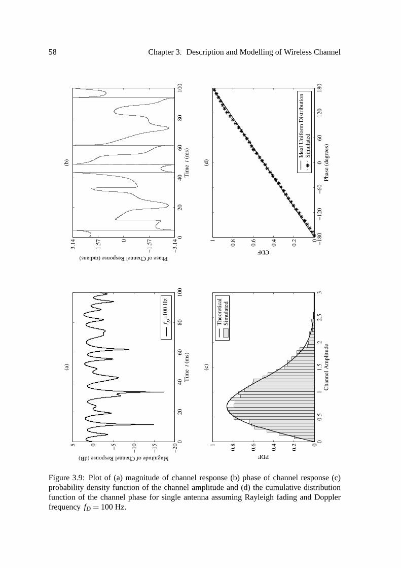
58 Chapter 3. Description and Modelling of Wireless Channel
020
4060
8010
0−2
0
−15
−10−505
Magnitude of Channel Response (dB)
Tim
e t
(ms)
(a)
f D=1
00 H
z
020
4060
8010
0−3
.14
−1.5
70
1.57
3.14
Phase of Channel Response (radians)
Tim
e t
(ms)
(b)
00.
51
1.5
22.
53
0
0.2
0.4
0.6
0.81
Cha
nnel
Am
plitu
de
(c)
The
oret
ical
Sim
ulat
ed
−180
−120
−60
060
120
180
0
0.2
0.4
0.6
0.81
Phas
e (d
egre
es)
CDF
(d) Id
eal U
nifo
rm D
istr
ibut
ion
Sim
ulat
ed
Figure 3.9: Plot of (a) magnitude of channel response (b) phase of channel response (c)probability density function of the channel amplitude and (d) the cumulative distributionfunction of the channel phase for single antenna assuming Rayleigh fading and DopplerfrequencyfD = 100 Hz.

3.3. Rayleigh Fading Channel Simulations 59
0 5
1015
2025
3035
40−3
0
−25
−20
−15
−10−505
Magnitude of Channel Response (dB)
Tim
e t
(ms)
(a)
0 5
1015
2025
3035
40−3
.14
−1.5
7
0
1.57
3.14
Phase of Channel Response (radians)
Tim
e t
(ms)
(b)
N =
1N
= 2
N =
3N
= 4
N =
1N
= 2
N =
3N
= 4
Figure 3.10: Plot of (a) magnitude and (b) phase of channel response forN = 4 antennaelements with inter-element spacingd = λ/2 assuming Rayleigh fading, mean AOAθ =20, Doppler frequencyfD = 100 Hz and no angle spread.
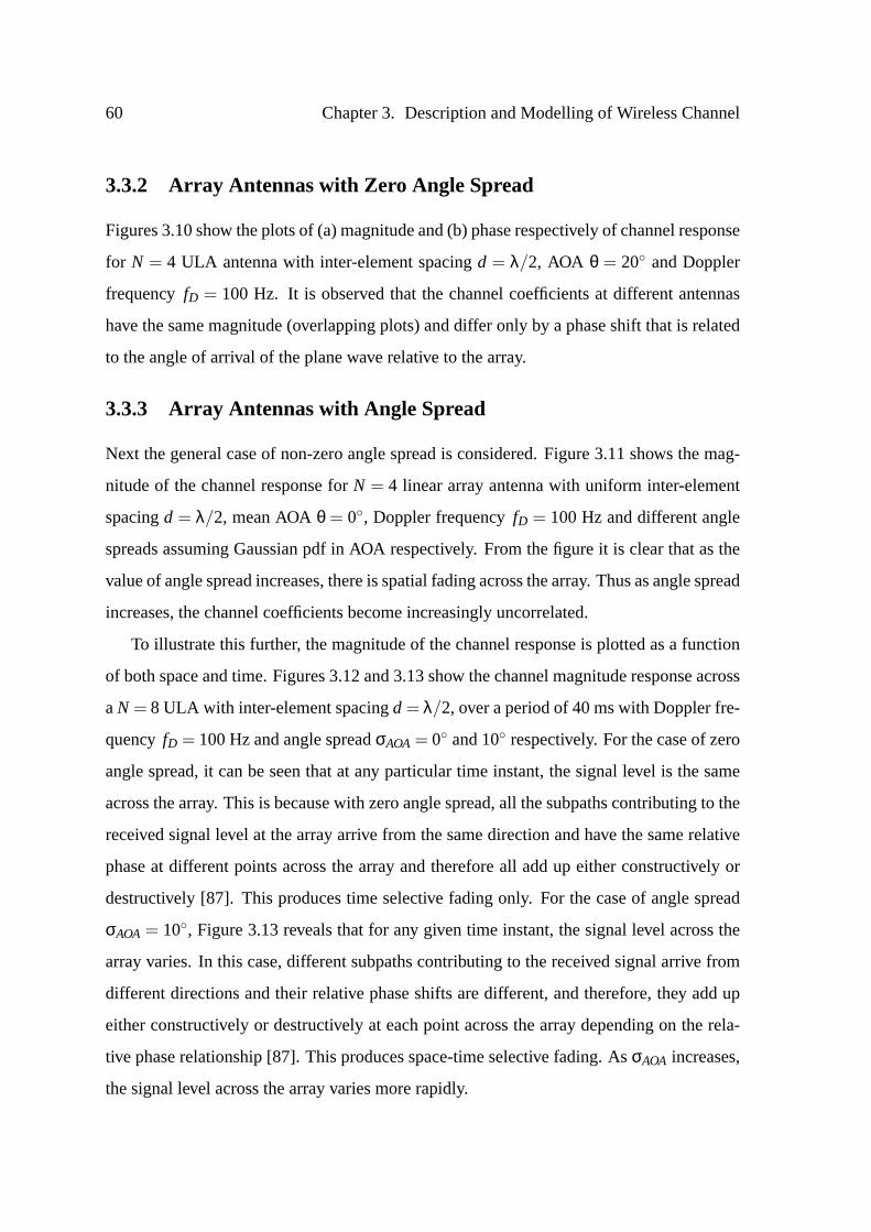
60 Chapter 3. Description and Modelling of Wireless Channel
3.3.2 Array Antennas with Zero Angle Spread
Figures 3.10 show the plots of (a) magnitude and (b) phase respectively of channel response
for N = 4 ULA antenna with inter-element spacingd = λ/2, AOA θ = 20 and Doppler
frequencyfD = 100 Hz. It is observed that the channel coefficients at different antennas
have the same magnitude (overlapping plots) and differ only by a phase shift that is related
to the angle of arrival of the plane wave relative to the array.
3.3.3 Array Antennas with Angle Spread
Next the general case of non-zero angle spread is considered. Figure 3.11 shows the mag-
nitude of the channel response forN = 4 linear array antenna with uniform inter-element
spacingd = λ/2, mean AOAθ = 0, Doppler frequencyfD = 100 Hz and different angle
spreads assuming Gaussian pdf in AOA respectively. From the figure it is clear that as the
value of angle spread increases, there is spatial fading across the array. Thus as angle spread
increases, the channel coefficients become increasingly uncorrelated.
To illustrate this further, the magnitude of the channel response is plotted as a function
of both space and time. Figures 3.12 and 3.13 show the channel magnitude response across
aN = 8 ULA with inter-element spacingd = λ/2, over a period of 40 ms with Doppler fre-
quencyfD = 100 Hz and angle spreadσAOA= 0 and 10 respectively. For the case of zero
angle spread, it can be seen that at any particular time instant, the signal level is the same
across the array. This is because with zero angle spread, all the subpaths contributing to the
received signal level at the array arrive from the same direction and have the same relative
phase at different points across the array and therefore all add up either constructively or
destructively [87]. This produces time selective fading only. For the case of angle spread
σAOA = 10, Figure 3.13 reveals that for any given time instant, the signal level across the
array varies. In this case, different subpaths contributing to the received signal arrive from
different directions and their relative phase shifts are different, and therefore, they add up
either constructively or destructively at each point across the array depending on the rela-
tive phase relationship [87]. This produces space-time selective fading. AsσAOA increases,
the signal level across the array varies more rapidly.

3.3. Rayleigh Fading Channel Simulations 61
0 5
1015
2025
3035
40−2
0
−15
−10−505
Magnitude of Channel Response (dB)
Tim
e t
(ms)
(a) A
OA
θ =
0°, σ
AO
A = 0
°
0 5
1015
2025
3035
40−2
0
−15
−10−505
Magnitude of Channel Response (dB)
Tim
e t
(ms)
(b) A
OA
θ =
0°, σ
AO
A = 5
°
0 5
1015
2025
3035
40−2
0
−15
−10−505
Magnitude of Channel Response (dB)
Tim
e t
(ms)
(c) A
OA
θ =
0°, σ
AO
A = 1
0°
0 5
1015
2025
3035
40−2
0
−15
−10−505
Magnitude of Channel Response (dB)
Tim
e t
(ms)
(d) A
OA
θ =
0°, σ
AO
A = 2
0°
N =
1N
= 2
N =
3N
= 4
N =
1N
= 2
N =
3N
= 4
N =
1N
= 2
N =
3N
= 4
N =
1N
= 2
N =
3N
= 4
Figure 3.11: Channel magnitude response forN = 4 antenna elements with inter-elementspacingd = λ/2 assuming Rayleigh fading, Gaussian pdf in AOA, mean AOAθ = 0 andangle spreadsσAOA = 0,5,10,20 respectively.

62 Chapter 3. Description and Modelling of Wireless Channel
0 10 20 30 40
01
23
4−20
−15
−10
−5
0
5
Time t (ms)Space (d/λ)
Mag
nitu
de o
f Cha
nnel
Res
pons
e (d
B)
Figure 3.12: Space-time fading:N = 8 antenna elements,d = λ/2, Doppler frequencyfD = 100 Hz and angle spreadσAOA = 0.
0 10 20 30 40
01
23
4−20
−15
−10
−5
0
5
Time t (ms)Space (d/λ)
Mag
nitu
de o
f Cha
nnel
Res
pons
e (d
B)
Figure 3.13: Space-time fading:N = 8 antenna elements,d = λ/2, Doppler frequencyfD = 100 Hz and angle spreadσAOA = 10.

3.4. Rician Fading Channel Simulations 63
3.4 Rician Fading Channel Simulations
The results in this section are obtained by implementing (3.31), using the simulation model
developed for the purpose (see Appendix B). The value ofL = 1 path is used in the simu-
lations. The following cases are considered:-
3.4.1 Effect of Rice Factor
Figure 3.14 shows the magnitude of the channel response with Rician fading for a total time
period oft = 200 ms and different Rician factorsKR =−∞,1,5,7,10 (dB) respectively. The
curve forKR = 0 (−∞ dB) corresponds to the case of Rayleigh fading. From the figure, it
is clear that asKR increases, the probability of encountering deep fades is reduced. Thus
a Rician channel is a more ‘friendly’ channel while the Rayleigh case represents a ‘worst-
case’ mobile channel, as the signal fading is more severe with deeper and more frequent
nulls.
3.4.2 Distribution of Channel Coefficients
Figure 3.15 shows the probability density histograms of the channel amplitude forKR =
−∞,1,5,10 dB respectively. The statistics of the channel amplitudes are collected over an
extended time period of 2.5 s (corresponding to 250λ). The theoretical Rice probability
density functions are also shown for comparison. It can be observed that there is a very
good match between the simulated and theoretical values. This result indicates that the
proposed model is able to accurately simulate Rician fading characteristics.
3.5 Summary
This chapter has presented a new parameterized physical channel model for use in per-
formance evaluation of smart antennas. The proposed model includes the temporal and
spatial propagation processes such as MS mobility, azimuth angle of arrival, angle spread
and Doppler frequency which are of critical importance for smart antenna systems. A
mathematical formulation of the channel model has also been presented, along with the

64 Chapter 3. Description and Modelling of Wireless Channel
050
100
150
200
−20020406080100
Magnitude of Channel Response (dB)
Tim
e t (
ms)
KR =
− ∞
dB
KR =
1 d
B
KR =
5 d
B
KR =
7 d
B
KR =
10
dB
Figure 3.14: Channel magnitude response for single antenna assuming Rician fading andRice factorsKR = −∞,1,5,7,10 dB respectively. Curves are offset upwards by 20 dB forincreasingKR values for clarity.

3.5. Summary 65
00.
51
1.5
22.
53
0
0.51
1.52
2.53
Cha
nnel
Am
plitu
de
(a) K
R =
−∞
dB
The
oret
ical
Sim
ulat
ed
00.
51
1.5
22.
53
0
0.51
1.52
2.53
Cha
nnel
Am
plitu
de
(b) K
R =
1 d
B
The
oret
ical
Sim
ulat
ed
00.
51
1.5
22.
53
0
0.51
1.52
2.53
Cha
nnel
Am
plitu
de
(c) K
R =
5 d
B
The
oret
ical
Sim
ulat
ed
00.
51
1.5
22.
53
0
0.51
1.52
2.53
Cha
nnel
Am
plitu
de
(d) K
R =
10
dB
The
oret
ical
Sim
ulat
ed
Figure 3.15: The probability density histograms of the channel amplitude assuming Ricianfading and Rice factorsKR =−∞,1,5,10 dB respectively.

66 Chapter 3. Description and Modelling of Wireless Channel
simulation results. It has been shown that the proposed channel model is able to accurately
simulate various Rayleigh and Rician fading scenarios. In addition, it has been shown that
angle spread produces spatial fading across the array, affording additional space diversity
gain. The proposed channel model is used to analyse and simulate the performance of smart
antenna systems in Chapters 4 and 5.

Chapter 4
Performance Evaluation of SmartAntennas for CDMA
In this chapter an analytical model for investigating the mean Bit Error Rate (BER) per-
formance of a Direct Sequence Code Division Multiple Access (DS-CDMA) system em-
ploying a smart antenna is described. The DS-CDMA system is assumed to utiliseM-ary
orthogonal modulation. As mentioned in Chapter 1, this type of modulation has been suc-
cessfully used in the reverse link of IS-95 CDMA system and is also specified in radio
configurations 1 and 2 of the reverse link in cdma2000 standard. The proposed model
incorporates the array and channel models developed in Chapters 2 and 3 respectively.
This chapter is organised as follows. The detailed system model is presented in Sec-
tion 4.1. The smart antenna receiver structure and its different blocks are described in
Section 4.2. The analysis results for noncoherentM-ary orthogonal modulation with single
antenna, which form the basis of the proposed model, are outlined in Section 4.3. Follow-
ing this, the analytical model is described in Section 4.4. The simulation assumptions and
Monte Carlo simulation strategy employed to simulate the performance of smart antennas
are discussed in Section 4.5. Finally, the analytical results are compared with simulation
results in Section 4.6 to validate the proposed model.
4.1 System Model
Consider a BS serving a single 120 angular sector. Without loss of generality, it is assumed
that the BS employs a Uniform Linear Array (ULA) ofN identical omni-directional antenna
67

68 Chapter 4. Performance Evaluation of Smart Antennas for CDMA
MSk
0°
1
−60° 60°
BS array antenna
MS1
MS2
MSK
2 3 4 5 N
θk
θ1
d
Figure 4.1: Smart antenna BS serving a single 120 angular sector of CDMA system.
elements, with inter-element spacing ofd = λ/2, as shown in Figure 4.1.
Let K denote the total number of active Mobile Stations (MS) in the system, which are
randomly distributed in the azimuthal direction, along the arc boundary of the sector cell
in the far field of the array. It is assumed that each MS usesM-ary orthogonal modula-
tion [159]. Thek = 1 user is assumed to be the desired user. For simplicity, an uncoded
system is considered i.e. the convolutional encoder and interleaver are ignored. This ap-
proach is widely used (see, for instance [30,34,82,83]) as it allows the analysis of wireless
communication systems employing multiple antennas. It has to be noted that, in practice,
channel coding is an essential component of DS-CDMA wireless communication systems.
The signals transmitted by theK users pass through a multipath channel and are received
by the BS array antenna. The location of each MS is characterized by its Angle of Arrival
(AOA) θk, which is conventionally measured from the array broadside.
The BS receiver consists of a two-dimensional (2-D) RAKE receiver [82] with a con-
ventional Maximum Signal to Noise Ratio beamformer [160] followed by anL finger non-
coherent RAKE combiner [161]. As mentioned in Chapter 1, the actual beamforming algo-
rithms used to determine the weights fall outside the scope of this thesis. Hence, the ideal
solution for the beamforming weight vectors is used. Also the RAKE receiver is assumed
to have perfect knowledge of the multipath delays.

4.1. System Model 69
RandomData Bits
Walsh CodeModulation
and Spreading
To
a(I)(t)
sk(t)
I-channel
Q-channel
a(Q)(t)
TransmitAntenna
ak(t)Long Code
Figure 4.2: Block diagram of mobile station transmitter.
4.1.1 Transmitter Model
The block diagram of the MS transmitter is shown in Figure 4.2, which is adapted from
Figure A.1 (see Appendix A). It employs Offset Quadrature Phase Shift Keying (OQPSK)
M-ary orthogonal modulation and closely follows the reverse link specifications of the IS-
95 CDMA [4,159]. The transmitted signalsk(t) of thekth user can be written as [82]
sk(t) = W(m)k (t)a(I)
k (t)cos(ωct)+W(m)k (t−To)a(Q)
k (t−To)sin(ωct) (4.1)
wherem= 1,2, . . . ,M,W(m)k (t) is a Hadamard-Walsh function of dimensionM which repre-
sents themth orthogonal signal of thekth user,a(I)k (t) = ak(t)a(I)(t), a(Q)
k (t) = ak(t)a(Q)(t),
ak(t) is thekth user’s long code sequence,a(I)(t) anda(Q)(t) are the in-phase and quadra-
ture channel Pseudo-Noise (PN) random sequences respectively,To is the half chip delay for
OQPSK signals,ωc = 2π fc and fc is the carrier frequency. The transmitted power of each
user is assumed unity. This reflects the assumption of perfect power control. To simplify
the analysis, the PN codes are represented by [77]
a(I)k (t) =
∞
∑r=−∞
a(I)k,r(t) p(t−Tc) (4.2)
a(Q)k (t) =
∞
∑r=−∞
a(Q)k,r (t) p(t−Tc) (4.3)
wherea(I)k,r anda(Q)
k,r are assumed to be independent and identically distributed (i.i.d.) ran-
dom variable taking values±1 with equal probability andp(t) is the chip pulse shape,
which is assumed to be rectangular.

70 Chapter 4. Performance Evaluation of Smart Antennas for CDMA
Re-writing the transmitted signal in (4.1), we get
sk(t) = ℜ
[W(m)k (t)a(I)
k (t)+ jW(m)k (t−To)a(Q)
k (t−To)]e− jωct
= ℜsk(t)e− jωct (4.4)
wheresk(t) = s(I)k (t)+ j s(Q)
k (t) is the complex low pass equivalent of the transmitted signal.
The two representations are equivalent [162] and are used interchangeably in this chapter.
4.1.2 Channel Model
Thekth user’s signal propagates through a multipath fading channel with Angle of Arrival
(AOA) θk. Using the channel model presented in Chapter 3, the complex lowpass equivalent
representation of the channel impulse response between thel th multipath of thekth user and
thenth element of the array antenna is given by
hk,l ,n(t) = βk,l e− j(φk,l +2π dλ (n−1)sinθk)δ(t− τk,l )
= βk,l e− jϕk,l ,nδ(t− τk,l ) (4.5)
whereβk,l , φk,l andτk,l are the path gain, phase and delay respectively,ϕk,l ,n is the overall
phase which includes the path phase and the difference in propagation delays between the
antennas andλ is the wavelength. The path gains are assumed to follow the Rayleigh or the
Rician distributions respectively. It is also assumed that the multipath channel parameters
βk,l (t) andϕk,l ,n(t) remain constant for the duration of a Walsh symbol [77]. Therefore,
βk,l (t) = βk,l andϕk,l ,n(t) = ϕk,l ,n for t ∈ [0,Tw], whereTw is Walsh symbol period.
4.1.3 Received Signal
Following [77], the total received signal at thenth antenna element can be written as
xn(t) =K
∑k=1
L
∑l=1
ℜ[sk(t−Γk)∗ hk,l ,n(t)]e−ωct+η(t)
=K
∑k=1
L
∑l=1
[βk,l W
(m)k (t− τk,l )a(I)
k (t− τk,l )cos(ωct +ϕk,l ,n)
+ βk,l W(m)k (t−To− τk,l )a(Q)
k (t−To− τk,l )sin(ωct +ϕk,l ,n)]+ηn(t) (4.6)

4.2. Smart Antenna Receiver Model 71
wheresk(t) is the signal transmitted bykth user given in (4.1),τk,l = Γk + τk,l , Γk is the
random delay of thekth user due to the asynchronous nature of the CDMA system andη(t)
is the Additive White Gaussian Noise (AWGN). The noise may be represented in terms of
its lowpass equivalent by
η(t) = ℜη(t)e− jωct (4.7)
whereη(t) = η(I)(t) + j η(Q)(t) and η(I)(t) and η(Q)(t) are the in-phase and quadrature
components ofη(t).
4.2 Smart Antenna Receiver Model
The functional block diagram of the smart antenna receiver is shown in Figure 4.3, which is
adapted and simplified from [82]. It has a Two-Dimensional (2-D) RAKE structure where
the multipath components are tracked in both time and space. From the figure, the following
main blocks can be identified (i) array antenna, (ii) PN despreading, (iii) beamforming and
(iv) Walsh correlation and demodulation. The function and modelling of these blocks is
explained below.
4.2.1 Extraction of Quadrature Components
The first step for the receiver is to obtain the quadrature components at each antenna. This
is achieved by multiplying the received waveforms by cos(ωct) and sin(ωct) respectively
and then lowpass filtering to remove the double frequency components that result from
multiplication [159]. The output of theI -channel andQ-channel lowpass filters can be
written as
x(I)k,l ,n(t) =
[xk,l ,n(t)cos(ωct)
]LPF
=
βk,l W(m)k (t− τk,l )a(I)
k (t− τk,l )cosϕk,l ,n
2
+βk,l W(m)k (t−To− τk,l )a(Q)
k (t−To− τk,l )sinϕk,l ,n
2
+
η(I)(t)2
(4.8)

72 Chapter 4. Performance Evaluation of Smart Antennas for CDMA
Dow
nC
onve
rsio
n
N
Fing
er 1
(PN
des
prea
ding
)
Fing
er
L(P
N d
espr
eadi
ng)
Dow
nC
onve
rsio
n
1
Fing
er 1
(PN
des
prea
ding
)
Fing
er
L(P
N d
espr
eadi
ng)
Arr
ayan
tenn
a
nk
L nn
ky
w,1,
*
1,1,
)(
∑ =
nL
k
N nn
Lk
yw
,,
*
1,
,)
(∑ =B
eam
form
ing
=L l
lk
u1
,
Wal
shC
orre
latio
n
Wal
shC
orre
latio
n
Wal
shD
emod
ulat
ion
BE
R
1,k
u Lk
u,
1,kz
Lkz
,
1,1,ky L
ky,1,
1,,L
ky
NL
ky,
,
Figure 4.3: Block diagram of smart antenna receiver.

4.2. Smart Antenna Receiver Model 73
x(Q)k,l ,n(t) =
[xk,l ,n(t)sin(ωct)
]LPF
=
βk,l W(m)k (t− τk,l )a(Q)
k (t−To− τk,l )cosϕk,l ,n
2
−βk,l W(m)k (t−To− τk,l )a(I)
k (t− τk,l )sinϕk,l ,n
2
+
η(Q)(t)2
(4.9)
Using the quadrature components, the complex lowpass equivalent of the received signal
can be written as
xk,l ,n(t) = x(I)k,l ,n(t)+ j x(Q)
k,l ,n(t) (4.10)
4.2.2 Despreading for Noncoherent Detection
After filtering, each resolvable path is then detected by one of the RAKE fingers immedi-
ately following the radio-frequency stages. To detect thel th path, the signal is despread
using the sequence of the respective mobile and synchronized to the delay of thel th path.
Additionally, the cross-correlation of theI andQ channels is found in order to noncoher-
ently combine the signals. Thus the in-phase signal is also correlated with the quadrature
arm and an equivalent operation performed for the quadrature signal, as shown in Fig-
ure 4.4 [159]. This process can be mathematically represented as follows.
Let the complex lowpass equivalent of the post PN-despread signal ˜yk,l ,n(t) be given as
yk,l ,n(t) = y(I)k,l ,n(t)+ j y(Q)
k,l ,n(t) (4.11)
Denoting the despreading sequences as ˜a(t) = [a(I)k (t − τk,l ) + j a(Q)
k (t −To− τk,l )] [107,
163], the quadrature components of ˜yk,l ,n can be written as
y(I)k,l ,n(t) = ℜ
(a(t), xk,l ,n(t)
)= x(I)
k,l ,n(t)a(I)k (t− τk,l )+x(Q)
k,l ,n(t)a(Q)k (t−To− τk,l ) (4.12)
y(Q)k,l ,n(t) = ℑ
(a(t), xk,l ,n(t)
)= x(I)
k,l ,n(t)a(Q)k (t−To− τk,l )−x(Q)
k,l ,n(t)a(I)k (t− τk,l ) (4.13)
where(a,b) = a·b∗ denotes the dot product between the complex numbers.
The post PN-despread signals can be written in vector notation as
yk,l = [ yk,l ,1 yk,l ,2 · · · yk,l ,N ]T (4.14)

74 Chapter 4. Performance Evaluation of Smart Antennas for CDMA
x(I)(t)
x(Q)(t)
ak(t-To-τ)
ak(t-To-τ)
a(Q)(t-To-τ)
a(Q)(t-To-τ)
ak(t-τ)
ak(t-τ) a(I)(t-τ)
a(I)(t-τ)
x(QQ)(t)
Low PassFilter
cos(ωct)
sin(ωct)
Low PassFilter
__
+
+
+
y(I)
x(t)
y(Q)
x(QI)(t)
x(IQ)(t)
x(II)(t)
Figure 4.4: Despreading for noncoherent detection ofM-ary orthogonal modulation.

4.2. Smart Antenna Receiver Model 75
4.2.3 Beamforming
A beamformer is then constructed for each resolvable multipath and the signal after PN
despreading is combined by the beamformer. In the beamforming operation, the signals
received by the antenna elements are weighted by complex weights and then summed up.
The smart antenna output is given by
zk,l (t) = (wk,l )H yk,l (t) (4.15)
= z(I)k,l + j z(Q)
k,l (4.16)
wherewk,l is the beamforming weight vector given by
wk,l = [ wk,l ,1 wk,l ,2 · · · wk,l ,N ]T (4.17)
It is assumed that the weights are determined using the Maximum Signal to Noise Ratio
(SNR) beamforming criteria [160]. As mentioned in Chapter 1, the actual mechanisms used
to determine the weights fall outside the scope of the thesis. Thus the weights are set as
wk,l = hk,l and these vector channel coefficients are assumed to be perfectly known. This
provides the best case system performance.
4.2.4 Walsh Correlation and Demodulation
The next step is the correlation of the smart antenna output with stored replicas of the Walsh
functions. This is required to form the decision variable for demodulation. The output of
theqth Walsh correlator (q = 1,2, · · · ,M) is given by
Z(I)k,l (q) =
1Tw
∫ Tw+τk,l
τk,l
[z(I)k,l W(q)(t− τk,l )+z(I)
k,l W(q)(t−To− τk,l )]dt (4.18)
Z(Q)k,l (q) =
1Tw
∫ Tw+τk,l
τk,l
[z(Q)k,l W(q)(t− τk,l )+z(Q)
k,l W(q)(t−To− τk,l )]dt (4.19)
The decision variable for thel th multipath of thekth user is obtained from the Walsh
correlated values as
uk,l (q) =(
Z(I)k,l
)2+(
Z(Q)k,l
)2(4.20)

76 Chapter 4. Performance Evaluation of Smart Antennas for CDMA
The overall decision variable is obtained by Equal Gain Combining (EGC) of all the
decision variables from theL multipaths as [79]
uk(q) =L
∑l=1
uk,l (q) =L
∑l=1
[(Z(I)
k,l
)2+(
Z(Q)k,l
)2]
(4.21)
Finally, the receiver makes a hard decision on themth symbol of thekth user by using
the Maximum Likelihood Criteria rule as
m= arg maxq=1,...,M
uk(q) (4.22)
4.3 Probability of Error Analysis for Single Antenna
Before considering the performance of the smart antenna system, discussed in the previous
section, the Mean BER performance of the conventional single antenna receiver (i.e.N = 1)
is examined. The results in this section form the basis of the proposed analytical model,
which is presented in the next section.
4.3.1 Variances
Following [77, 79], it can be shown that for a single antenna, the output of theqth Walsh
correlator (q = 1,2, · · · ,M) can be written as
Z(I)k,l (q) =
βk,l cosϕk,l + I (I)
k,l +M(I)k,l +N(I)
k,l ; if q = m
I (I)k,l +M(I)
k,l +N(I)k,l ;else
(4.23)
Z(Q)k,l (q) =
βk,l sinϕk,l + I (Q)
k,l +M(Q)k,l +N(Q)
k,l ; if q = m
I (Q)k,l +M(Q)
k,l +N(Q)k,l ;else
(4.24)
whereN(I)k,l andN(Q)
k,l denote the noise terms,M(I)k,l andM(Q)
k,l denote the MAI terms andI (I)k,l
andI (Q)k,l denote the self interference terms.
The Gaussian approximation is used for the noise and interference terms [80]. The
Gaussian approximation does not always hold for CDMA analyses. However for largeNc,
this approximation has been shown to give reasonable results [164]. Using this approxi-
mation, it can be shown that the multiple access interferences termsM(I)k,l andM(Q)
k,l can be

4.3. Probability of Error Analysis for Single Antenna 77
modelled as zero mean Gaussian random processes with variance [79]
σ2M =
Es
3Nc
K−1
∑k=1
L
∑l=1
E[(βk,l )2] (4.25)
whereEs = Eb log2(M) is the symbol energy,Eb is the bit energy andNc = Tw/Tc is the
spreading factor.
I (I)k,l andI (Q)
k,l are the respective self interferences due to the desired users own multipaths
and can be modelled as zero mean Gaussian random processes with variance [79]
σ2I =
Es
3Nc
L−1
∑l=1
E[(βk,l )2] (4.26)
The noise termsN(I)k,l andN(Q)
k,l are mutually independent zero mean Gaussian random
processes with variance
σ2N =
No
2(4.27)
whereNo is the noise PSD.
The decision variable in (4.21) is a sum of squares of two Gaussian random variables,
each with variance
σ2T = σ2
N +σ2I +σ2
M
=No
2+
Es
3Nc
L−1
∑l=1
E[(βk,l )2]+K−1
∑k=1
L
∑l=1
E[(βk,l )2]
(4.28)
It is assumed that uniform power delay profile is used to characterize the multipath
fading channel and that all users have the same average signal power at the receiver due to
perfect power control, i.e.Ωk,1 = Ωk,2 = · · ·= Ωk,L = Ω/L. Therefore, (4.28) becomes
σ2T =
No
2+
Es
3Nc
ΩL
(L−1)+Es
3Nc
ΩL
(K−1)L
=No
2+
Es
3Nc
ΩL
(KL−1) (4.29)
The SINR can thus be written as
ρ =ΩL
Es
2σ2T
=γ
1+ 23Nc
γ(KL−1)(4.30)
whereγ = ΩL
EsNo
= ΩL
EbNo
log2(M).

78 Chapter 4. Performance Evaluation of Smart Antennas for CDMA
4.3.2 Decision Statistics and Error Probability
Using the SINR in (4.30), the BER of the single antenna system can be derived. Follow-
ing [79], it can be shown that when the desired signal is not present (i.e.q 6= m), the
decision variableuk(q) in (4.21) has a chi-square distribution with 2L degrees of freedom
and its probability density function (pdf) is given by
fuk(q)(z) =1
(2σ2T)L (L−1)!
zL−1exp
(− z
2σ2T
)(4.31)
When the desired signal is present (i.e.q = m), the decision variableuk(q) has a non-
central chi-square distribution with 2L degrees of freedom and noncentrality parameter
c = Es
L
∑l=1
(βk,l )2 (4.32)
Therefore given the path gainsβk,l , the conditional probability density function of the deci-
sion variableuk(q) is given by
fuk(q)(z|c) =1
2σ2T
(zc
) L−12
exp
(−z+c
2σ2T
)IL−1
(√zc
σ2T
)(4.33)
whereσ2T is given in (4.29) andIL−1(·) is the modified Bessel function of orderL−1. The
conditioning in (4.33) may be removed using
fuk(q)(z) =∫ ∞
0fuk(q)(z|c) f (c) dc (4.34)
where f (c) is the pdf ofc.
The receiver uses maximum likelihood decision rule and chooses the largest among the
decision variables. We assume without loss of generality thatm= 1, i.e. the first Walsh
symbolW(1)(t) is transmitted. Then the probability of symbol error is
PM = 1−Pc
= 1−P(uk(2) < uk(1), uk(3) < uk(1), . . . , uk(M) < uk(1))
= 1−∫ ∞
0[P(uk(2) < z1 |uk(1) = z1)]M−1 fuk(1)(z1) dz1 (4.35)
wherePc is the probability of correct decision. Finally the corresponding BER can easily
be obtained using the relationship [159]
P(1-D)b =
2K−1
2K −1PM =
M/2M−1
PM (4.36)

4.3. Probability of Error Analysis for Single Antenna 79
The results, obtained by evaluating and simplifying (4.35) for the commonly used
Rayleigh and Rician fading distributions, are given below:-
4.3.2.1 Rayleigh Fading
For the case of Rayleigh fading, it can be shown that the mean BER for a conventional one-
dimensional (1-D) RAKE receiver (i.e. single antenna without beamforming) withL-fold
multipath diversity and Equal Gain Combining (EGC) is given by [159]
P(1-D)b =
M/2M−1
M−1
∑m=1
(M−1
m
)(−1)m+1
(1+m+mρ)L
m(L−1)
∑l=0
Cl (m)(
L+ l −1l
)(1+ρ
1+m+mρ
)l
(4.37)
whereρ is given in (4.30) and the coefficientsCl (m) can be computed recursively us-
ing [159]
Cl (m) =
1l
l∑
q=1
( lq
)[(m+1)q− l ]Cl−q(m) ; l ≤ L−1,
1l
L−1∑
q=1
( lq
)[(m+1)q− l ]Cl−q(m) ; l ≥ L−1.
(4.38)
with C0(m) = 1 for all m.
For the special case of no multipath diversity (i.e.L = 1), (4.37) reduces to
P(1-D)b =
M/2M−1
M−1
∑m=1
(M−1
m
)(−1)m+1
1+m+mρ
whereρ is given by substitutingL = 1 in (4.30) and its value isρ = γ1+ 2
3Ncγ(K−1)
.
4.3.2.2 Rician Fading
For the case of Rician fading withL = 1, it can be shown that the mean BER for a conven-
tional 1-D RAKE receiver (i.e. single antenna without beamforming) is given by [165]
P(1-D)b =
M/2M−1
M−1
∑m=1
(M−1
m
)(−1)m+1
(1+m+mδ1)exp
(−δ1
1+m+mδ2
)(4.39)
where the variablesδ1 andδ2 are given by
δ1 =ρ
1+ 1KR
(4.40)
δ2 =ρ
1+KR(4.41)

80 Chapter 4. Performance Evaluation of Smart Antennas for CDMA
andρ is given by substitutingL = 1 in (4.30) andKR is the Rice factor given in (3.5).
4.4 Probability of Error Analysis for Array Antennas
The performance analysis of CDMA systems with smart antennas can be carried out by
following the same approach as outlined in the previous section for the case of the con-
ventional receiver. However, the inclusion of the complex beamformer weights in (4.15)
significantly complicates the mathematical analysis. As discussed in Section 1.4.3, various
BER approximation techniques have been proposed in order to analyse the mean BER of
the CDMA system with smart antennas. In this thesis the BER approximation procedure
for generic 2-D RAKE receivers described in [85] is followed.
4.4.1 BER Approximation Procedure
The BER approximation proposes to adapt the single antenna performance bounds (which
have been presented in Section 4.3) to array antenna systems. This is achieved by manipu-
lating those terms in the error probability formulas for single antenna receivers that account
for the noise and MAI. The following assumptions are made [85,86,166]:-
• The interferers are uniformly distributed in the coverage area comprising an angular
sector of 120.
• The interferers are partitioned into two spatial equivalence classes [167]− in-beam
and out-of-beam− based on whether their Angles of Arrivals lie inside or outside
the beam formed toward the desired user.
• A piece-wise beampattern is used to approximate the actual ULA beampattern. In the
pass band (or in-beam) the beampattern is modelled by a triangular function while
in the stop-band (or out-of-beam) the beampattern is approximated by a constant
attenuation factor representing an average side-lobe level.
• Because of the piece-line approximation, the energy of each in-beam interferer is a
random variable uniformly distributed within[12,1] (half power beamwidth region).
Hence a correction factor ofυ = 3/4 (average value) is applied for in-beam interfer-
ers.

4.4. Probability of Error Analysis for Array Antennas 81
−θBW 0 θ
BW
αo
00 dB
−∆θ = −60° ∆θ = 60°
Out−of−beamInterferers
Desired UserIn−beam Interferer
Out−of−beam Interferers
αo
Array Antenna
Actual ULA Beampattern
ApproximatedBeampattern
−3 −3
Figure 4.5: Illustration of the beampattern approximation and partitioning of interferers.
• For the purpose of evaluation of the error probability, the in-beam interferers are
counted as interference while the out-of-beam users increase the additive noise level.
The beampattern assumption and the partitioning of interferers is illustrated in Fig-
ure 4.5.
4.4.1.1 Mathematical Expression for Mean BER
Using the above model, it can be shown that the average bit error probability of a generic
2-D RAKE receiver is given by [85]
P(2-D)b =
K−1
∑κ=0
χξκ(
K−1κ
)P(1-D)
b (4.42)
whereκ denotes the number of in-beam interferers,(K−κ−1) is the number of out-of-
beam interferer,P(1-D)b is the probability of bit error for the scalar (single) antenna receiver
andχ and the probability of an in-beam interfererξ, are defined as [85]
ξ =(2θBW)
∆θ(4.43)
χ = (1−ξ)K−κ−1 (4.44)

82 Chapter 4. Performance Evaluation of Smart Antennas for CDMA
Table 4.1: Equivalent beamforming parameters
Number of antenna elementsN 4 6 8
Attenuationαo (dB) -12 -14 -16
Beamwidth 2θBW (degs.) 30 20 15
where∆θ = 120 is the total coverage angle of the sector and 2θBW is the total beamwidth
towards the desired user. The optimized values of equivalent beamforming parameters
2θBW andαo used in this work are given in Table 4.1 [85].
(4.42) can be adapted to different receivers depending on the probability of bit error of
the scalar receiver. In the next section, this approximation is applied and extended to the
case of a 2-D RAKE receiver for CDMA with noncoherentM-ary orthogonal modulation.
4.4.2 Modified Variances
Let the modified variances of the noise, self interference and MAI be denoted asσ2N, σ2
I and
σ2M respectively.
Partitioning the interferers into in-beam and out-of-beam categories, we have
σ2M =
out-of-beam︷ ︸︸ ︷αo
Es
3Nc
ΩL
(K−κ−1)L
+
in-beam︷ ︸︸ ︷υ
Es
3Nc
ΩL
κL
(4.45)
whereαo is the attenuation factor for out-of-beam interferers andυ = 3/4 is a correction
factor for in-beam interferers.
Since the spatial channel in (4.5) is based on one AOA only, the self interference due
to desired user’s multipaths cannot be reduced by beamforming. Hence we haveσ2I = σ2
I ,
whereσ2I is given in (4.26).
In comparison with the power of the desired signal, the noise power at the output of
the antenna array is reduced byN times [37], whereN is the number of antenna elements.
Hence,
σ2N =
σ2N
N=
No2
N(4.46)

4.5. General Simulation Assumptions 83
The modified SINR at the output of the 2-D RAKE receiver is thus given byρ = Es2σ2
T, where
σ2T = σ2
N + σ2I + σ2
M is the total variance. Substituting the values and simplifying, we get
ρ =γ
1N + 2γ
3Nc[(L−1)+αo(K−κ−1)L+υκL]
(4.47)
where averageEb/No of each multipath isγ = ΩL
EsNo
= log2(M)ΩL
EbNo
.
4.4.3 Mean BER
The mean BER of the smart antenna system is given by [85]
P(2-D)b =
K−1
∑κ=0
χξκ(
K−1κ
)P(1-D)
b (4.48)
whereP(1-D)b is given by (4.37) for Rayleigh fading and (4.39) for Rician fading respectively,
ρ is given in (4.47),χ andξ are given in (4.43) and the equivalent beamforming parameters
2θBW andαo are given in Table 4.1 [85].
4.5 General Simulation Assumptions
Monte Carlo simulations [168, 169], based on the system model presented in Sections 4.1
and 4.2, are performed to confirm the validity and accuracy of the analytical model pre-
sented in Section 4.4. It has to be noted that the analytical model is applicable to both 2G
IS-95 CDMA system and 3G cdma2000 system (radio configurations 1 and 2) respectively.
However for the purpose of simulations, an uncoded IS-95 CDMA system with alphabet
sizeM = 64 and spreading gainNc = 256 is considered for simplicity to reduce the sim-
ulation times (see Appendix B). The following assumptions are made with respect to the
system parameters:-
• Cell layout
A single 120 angular sector is considered for compatibility with the tri-sectored
approach used by most of the current wireless communication systems.
• Number of users
The number of active usersK is varied in the range 1−20. UserK = 1 is assumed
to be the desired user.

84 Chapter 4. Performance Evaluation of Smart Antennas for CDMA
• Frame length
A frame length of 576 bits is used. This frame size is consistent with specifications
of IS-95 maximum data rate of 9600 bps at the output of the convolutional encoder.
• Asynchronous user delay
The random asynchronous user delay for each interferer is assumed to be uniformly
distributed over the interval[0,Tc], whereTc is the chip period. An over-sampling
factor ofQ = 4 is used (i.e. there are 4 samples/chip).
• Spreading sequences
The spreading sequences used are PN random sequences. The characteristic poly-
nomials used for generating the long code PN sequence and the in-phase and the
quadrature short code PN sequences are [4]
a(x) = x42+x35+x31+x27+x26+x25+x22+x21+x19 (4.49)
+ x18+x17+x16+x10+x6 +x5 +x3 +x2 +x+1
a(I)(x) = x15+x13+x9 +x8 +x7 +x5 +1 (4.50)
a(Q)(x) = x15+x12+x11+x10+x6 +x5 +x4 +x3 +1 (4.51)
The total processing gain of the system is equal toNc = 256.
• Channel environments
The following two distinct operating environments are considered:-
1. Rician fading withL = 1 path. This situation can occur in the case of urban
micro cell with LOS propagation.
2. Rayleigh fading withL = 1,2,3 multipaths respectively. This situation corre-
sponds to the case of urban or sub-urban macro cell with NLOS propagation.
It is assumed that all multipaths fade independently i.e. the effect of correlated
fading is not considered.
• Power delay profile
A uniform power delay profile is assumed. The two- and three-ray power delay
profiles used in the simulations have been discussed in Section 3.1.5 and are shown
specifically in Figure 3.4. The total average multipath power is normalized to one for
each user.

4.5. General Simulation Assumptions 85
• Doppler frequency
The maximum Doppler frequency considered isfD = 100 Hz in all cases. This cor-
responds to a fast vehicular channel.
• User locations
The desired user is assumed to be located at−60 at the start of the simulation.
The desired user then moves with angle change∆θ = 0.01 per snapshot to cover
the entire azimuth range[−60, 60]. The interferers are assumed to be uniformly
distributed in angle throughout the sector.
• User mobility
To simulate MS mobility, the snapshot rate is assumed equal to the Walsh symbol
rate and the angle change between snapshots is∆θ = 0.01 per snapshot. This value
corresponds to a worst case scenario e.g., a fast moving MS at very close distance to
the BS and is widely used in the simulation studies, as discussed in Section 3.1.10.
• Power control
All the signals from theK users are assumed to arrive at the BS with the same power
level i.e. an ideal power control scenario is assumed.
• RAKE fingers
It is assumed that the 2-D RAKE receiver employs three fingers, i.e. all multipath
energy is assumed to be captured by the receiver. Also the multipath delays are
assumed to be perfectly estimated by the 2-D RAKE receiver.
• Adaptive array antenna
BS employs a Uniform Linear Array (ULA) ofN identical omni-directional antenna
elements, with inter-element spacing ofd = λ/2, to receive the signals.
• Weight vector adaptation
The smart antenna weight vector adaptation rate (snapshot rate) is assumed equal to
Walsh symbol rate. Also the weight vector is assumed to match perfectly with the
channel response vector i.e. the effect of imperfect adaptation is not considered.
The main simulation parameter values, as discussed above, are summarized in Table 4.2.

86 Chapter 4. Performance Evaluation of Smart Antennas for CDMA
Table 4.2: Main parameters for smart antenna simulations
Category Parameter Description or value
Monte Carlo Number of drops 50−100
Minimum number of bit errors 100
General Cellular layout Single 120 angular sector
Power control Ideal
Channel coding No
Oversampling factor Q = 4
Pulse shaping No
Detection Noncoherent
IS-95 CDMA Chip time Tc = 11228800s
Modulation OQPSK
Frame length 20 ms
Bits/frame 576
Base station synchronisation Asynchronous operation
Spreading codes Long code and I and Q channel
sequences
Number of users K = 1−20
Smart Antenna Antenna geometry Uniform linear array
Number of antenna elements N = 1,4,6,8
Inter-element distance d = λ/2
Element pattern Omnidirectional
Angle of Arrival −π/3≤ θ≤ π/3
User motion 0.01 per snapshot
Smart antenna adaptation perfect
Multipath Fading Fading distributions Rayleigh or Rician
Channel Number of subpaths S= 15
pdf in AOD Uniform
Number of multipaths L = 1,2,3
Power Delay Profile Uniform (two- and three-path)
Noise AWGN
Doppler frequency fD = 100 Hz

4.6. Results 87
4.5.1 Simulation Strategy
In order to generate performance results that represent an average measure of the cellular
system’s performance, the following Monte Carlo simulation strategy is adopted:-
• A simulation ‘drop’ [71] is defined as the transmission and reception of 125 frames,
which corresponds to the time required by the desired user to traverse the entire
azimuth range[−60, 60] with angle change∆θ = 0.01 per snapshot.
• In each simulation run over the variable of interest (e.g.Eb/No or K or N), the
number of bit errors is collected over a minimum of 50 drops. If the number of bit
errors exceeds the specified minimum number of bit errors (i.e. 100 [169]), then the
simulation is terminated and the mean BER is calculated. Otherwise, the simulations
are continued until at least 100 bit errors have been detected or the number of drops
reaches a maximum ofMc = 100. This upper limit on the number of drops is imposed
to limit the overall simulation time.
• At the beginning of each drop, the desired user’s AOA is set to−60, while the
AOA’s of the interferers are uniformly randomly distributed over the azimuth sector
range. Also the fading parameters for the multipaths are appropriately initialised as
discussed in Section 3.1.
• During a drop, the MS’s AOA increases or decreases linearly with angle change∆θ.
Also the channel undergoes fast fading according to the motion of the MS’s.
This procedure ensures that the BER performance of the system is averaged over the
ensemble of channel parameters and AOA of the multiple users and is not conditioned on a
particular spatial or temporal state of the system.
4.6 Results
The analytical results in this section are generated using (4.48) while the simulation results
are obtained by using the simulation model developed for the purpose (for details, see
Appendix B).

88 Chapter 4. Performance Evaluation of Smart Antennas for CDMA
0 5 10 15 2010−4
10−3
10−2
10−1
100
Eb/N
o (dB)
Mea
n B
it E
rror
Rat
e
↓ K = 1
↓ K = 15
L = 1 (anal. mod.) L = 2 (anal. mod.) L = 3 (anal. mod.) L = 1 (sim.) L = 2 (sim.) L = 3 (sim.)
Figure 4.6: Mean BER vs.Eb/No for N = 1 antenna, assumingK = 1,15 users,L = 1,2,3Rayleigh fading paths/user respectively (lines: analytical model, markers: simulations).
4.6.1 Single Antenna
First we take a look at the results for the case of a conventional single antenna receiver. Fig-
ure 4.6 shows a plot of Mean BER vs.Eb/No for N = 1 antenna, assumingK = 1,15 users
andL = 1,2,3 Rayleigh fading paths/user respectively. It can be seen that the simulation
results (markers) show good agreement with analytical results (lines). The single antenna
results serve as a reference for assessing the impact of smart antennas.
4.6.2 Rician Fading
The next case considered is the performance of smart antenna system, with parameters
specified in Table 4.2, operating in a Rician fading environment withL = 1.

4.6. Results 89
0 2.5 5 7.5 1010−7
10−6
10−5
10−4
10−3
10−2
10−1
100
Eb/N
o (dB)
Mea
n B
it E
rror
Rat
e
↓ N = 1
↓ N = 6
N = 6, KR= 1,5,7,10 dB
N = 1,6, Rayleigh (anal. mod.) N = 1,6, Rayleigh (sim.) N = 6, Rician (anal. mod.) N = 6, Rician (sim.)
10 dB
7 dB
5 dB
1 dB
Figure 4.7: Mean BER vs.Eb/No (dB) for N = 6 antennas,K = 1 user,L = 1 path/user, as-suming Rayleigh and Rician fading channels respectively (lines: analytical model, markers:simulations).
4.6.2.1 Effect of of varying the noise level for single user
Figure 4.7 shows the Mean BER vs.Eb/No (dB) for N = 6 antennas,K = 1 user with
single path assuming Rician fading with Rice factorKR = 1,5,7,10 dB respectively. The
performance in Rayleigh fading (corresponding toKR = −∞ dB) and the performance of
conventional receiver (i.e.N = 1 with no beamforming) are also shown as reference. From
this figure, it can be seen that beamforming improves the performance of the system. For
low values of Rice factor, the performance is very close to the performance in Rayleigh
fading. However for larger Rice factors, there is a tremendous improvement in the Mean
BER, e.g. forEb/No = 5 dB, a Rician factor ofKR = 5 dB improves the BER by a factor of
approximately 4 as compared to the case of Rayleigh fading. The simulation results (mark-
ers) show excellent agreement with analytical results (lines) for the different combinations
of Eb/No and Rician factorsKR.

90 Chapter 4. Performance Evaluation of Smart Antennas for CDMA
4.6.2.2 Effect of of varying the number of users
Figure 4.8 shows the Mean BER vs. Number of usersK for Eb/No = 10 dB,N = 6 antennas,
L = 1 path/user, assuming Rician fading with different Rice factors. The reference curves
for single antenna and Rayleigh fading are also shown in the figure. The figure shows that
as the number of users increases, the performance of the system gradually deteriorates.
This is to be expected as CDMA systems are interference limited systems. However, as
for the case of a single user, there is an improvement in performance with the increase in
KR, e.g. forK = 15 users, a Rician factor ofKR = 5 dB improves the BER by a factor of
approximately 4 over the Rayleigh fading case.The figure shows that the analytical model
provides a good match with simulation results for multi-user scenarios as well.
4.6.2.3 Effect of varying the number of antennas in multiple user scenario
Figure 4.9 shows the Mean BER vs. Number of antennasN, for Eb/No = 10 dB,K = 15
users assuming Rician fading with different Rice factors. The figure shows that doubling
the number of antennas from 4 to 8 improves the BER by a factor of approximately two
only, for values of Rician factor up to 5 dB (e.g. 1.9 forKR = −∞ dB, 1.9 forKR = 1 dB
and 2.2 forKR = 5 dB). However, for higher values of Rician factors the order of BER
improvement is greater than two, depending upon the value ofKR (e.g. 2.9 forKR = 7
dB and 5.4 forKR = 10 dB). This observation is of value in the planning of smart antenna
structures for urban micro cellular areas. It can also be seen again that the simulation
results show excellent agreement with the analytical results for the different combinations
of number of antennasN and Rician factorsKR.
4.6.3 Rayleigh Fading
Finally, the performance of the smart antenna system in Rayleigh fading multipath environ-
ment is examined.

4.6. Results 91
1 5 10 15 2010−7
10−6
10−5
10−4
10−3
10−2
10−1
100
Number of users K
Mea
n B
it E
rror
Rat
e
↓ N = 1
↓ N = 6
N = 6, KR=1,5,7,10 dB Rayleigh (anal. mod.)
Rayleigh (sim.)Rician (anal. mod.)Rician (sim.)
10 dB
7 dB
5 dB1dB
Figure 4.8: Mean BER vs. Number of usersK for Eb/No = 10 dB,N = 6 antennas,L = 1path/user, assuming Rayleigh and Rician fading channels respectively (lines: analyticalmodel, markers: simulations).
4 5 6 7 810−6
10−5
10−4
10−3
10−2
10−1
Number of Antennas N
Mea
n B
it E
rror
Rat
e
Rayleigh
K = 15, Rayleigh (anal. mod.) K = 15, Rayleigh (sim.) K = 15, Rician (anal. mod.) K = 15, Rician (sim.)
KR=10 dB
KR= 7 dB
KR= 5 dB
KR= 1 dB
Figure 4.9: Mean BER vs. Number of antennasN, for Eb/No = 10 dB,K = 15 users,L = 1path/user, assuming Rayleigh and Rician fading channels respectively (lines: analyticalmodel, markers: simulations).

92 Chapter 4. Performance Evaluation of Smart Antennas for CDMA
4.6.3.1 Effect of varying the number of users
Figure 4.10 shows the Mean BER vs. Number of usersK for Eb/No = 10 dB, assuming
L = 1,2 Rayleigh fading multipaths andN = 1,4,6,8 antennas respectively. Comparing
with the reference curves for single antenna (N = 1), it is clear that beamforming improves
the performance of the system considerably, e.g. forK = 20 users andL = 2 paths/user,
a N = 4 element smart antenna system improves the BER by a factor of approximately 8
as compared to the performance of a conventional receiver. It can be seen from the figure
that as the number of users increases, the analytical model provides a closer match with
simulation results, especially for the case ofL = 2 paths/user. This behaviour is further
illustrated in the next figure.
4.6.3.2 Effect of varying the noise level in a multiple user scenario
Figure 4.11 shows the mean BER versusEb/No (dB) with N = 8 antennas,K = 5,20 users
and L = 2,3 paths/user respectively. It can be seen that forK = 5 users the simulation
results (markers) are close to the analytical results (lines). However forK = 20 users,
which represents a more realistic mobile communications scenario, the simulation results
provide an even better agreement with the results obtained by the analytical model. This is
because the average BER performance predicted by the analytical model in (4.48) is highly
sensitive to the number of in-beam interferers. Consequently, as the number of users and
hence the probability of in-beam interferers increases, the prediction matches more closely
with the simulations.
4.6.3.3 Effect of varying the number of antennas
Figure 4.12 shows the Mean BER vs. Number of antennasN, for Eb/No = 10 dB,K = 15
users, assumingL = 1,2,3 Rayleigh fading multipaths. The figure shows that doubling the
number of antennas from 4 to 8 improves the BER by a factor that increases asL increases,
e.g. (approximately) 1.9 forL = 1, 3.0 forL = 2 and 3.7 forL = 3. Thus the number of
multipaths has a significant effect on the performance of the smart antenna system. It can
be seen again that the simulation results agree well with the analytical results.

4.6. Results 93
1 5 10 15 2010−5
10−4
10−3
10−2
10−1
100
Number of users K
Mea
n B
it E
rror
Rat
e
↓ L = 1
↓ L = 2
↓ N = 1
L = 1
L = 2
N = 1 (anal. mod.) N = 4 (anal. mod.) N = 4 (sim.) N = 6 (anal. mod.) N = 6 (sim.) N = 8 (anal. mod.) N = 8 (sim.)
Figure 4.10: Mean BER vs. Number of usersK for Eb/No = 10 dB, assumingL = 1,2Rayleigh fading paths/user andN = 1,4,6,8 antennas respectively (lines: analytical model,markers: simulations).
0 5 10 15 20 2510−7
10−6
10−5
10−4
10−3
10−2
10−1
Eb/N
o (dB)
Mea
n B
it E
rror
Rat
e
L = 3, K = 5
L = 2, K = 5
L = 3, K = 20
L = 2, K = 20
L=2, K=5 (anal. mod.) L=2, K=20 (anal. mod.) L=3, K=5 (anal. mod.) L=3, K=20 (anal. mod.) L=2, K=5 (sim.) L=2, K=20 (sim) L=3, K=5 (sim.) L=3, K=20 (sim.)
Figure 4.11: Mean BER vs.Eb/No for N = 8 antennas, assumingK = 5,20 users andL =2,3 Rayleigh fading paths/user respectively (lines: analytical model, markers: simulations).

94 Chapter 4. Performance Evaluation of Smart Antennas for CDMA
4 5 6 7 810−4
10−3
10−2
10−1
100
Number of antennas N
Mea
n B
it E
rror
Rat
e
K = 15 users L = 1 (anal. mod.) L = 1 (sim.) L = 2 (anal. mod.) L = 2 (sim.) L = 3 (anal. mod.) L = 3 (sim.)
Figure 4.12: Mean BER vs. Number of antennasN, for Eb/No = 10 dB,K = 15 users, as-sumingL = 1,2,3 Rayleigh fading paths/user respectively (lines: analytical model, mark-ers: simulations).
4.7 Summary
In this chapter, the performance of smart antennas for CDMA with noncoherentM-ary
orthogonal modulation in Rayleigh and Rician fading environments has been analysed. A
simple analytical model has been proposed which permits the BER to be readily evaluated
using a closed-form expression. The results obtained using this analytical model show good
agreement with the (computationally intensive) Monte Carlo simulation results. Thus the
analytical model can be used to rapidly calculate the smart antenna system performance
under a variety of user and channel scenarios and is of value in the planning of smart
antenna systems for urban and suburban areas.

Chapter 5
Performance of HierarchicalBeamforming for CDMA
In the last chapter, it has been shown that a smart antenna can mitigate Multiple Access
Interference (MAI) by beamforming or spatial filtering operation i.e. a smart antenna en-
hances the signal from the desired user (array gain in the direction of the desired user) and
discriminates against interferers located outside the main beam (beamforming gain). As
mentioned in Chapter 1, the performance of a CDMA system is limited by MAI and fast
fading. Traditionally, widely separated diversity antennas have been used to mitigate fad-
ing. In this chapter a hybrid scheme of diversity and smart antennas called Hierarchical
Beamforming (HBF) is investigated for an IS-95 CDMA system, to jointly combat fading
and MAI.
This chapter is organised as follows. In Section 5.1, the system model for the math-
ematical characterisation of HBF is presented. The HBF receiver model is described in
Section 5.2. The simulation strategy employed to simulate the performance of HBF is dis-
cussed in Section 5.3. Finally, in Section 5.4 the simulation results are presented and the
performance of HBF is compared with Conventional Beamforming (CBF).
5.1 System Model
Consider a BS serving a single 120 angular sector. It is assumed that the BS is equipped
with F co-linear sub-beamforming arrays. The number of array elements in each sub-
array isB. Thus the total number of array elements isN = F ×B. Each sub-array has an
95

96 Chapter 5. Performance of Hierarchical Beamforming for CDMA
sub-array #1 sub-array #2
1 2 B B21
w(2)k,l,1
d=λ/2ds>>λ
BS
w(2)k,l,2 w(2)
k,l,Bw(1)k,l,1 w(1)
k,l,2 w(1)k,l,B
Figure 5.1: Hierarchical beamforming array geometry.
inter-element spacing ofd = λ/2, while the spacing between the adjacent sub-arrays (ds) is
assumed large enough (e.g. 20λ or more) to ensure uncorrelated fading. This model is also
applicable to CBF. Specifically, the extreme case ofF = 1 andB = N corresponds to CBF.
The array geometry is illustrated in Figure 5.1 for the case ofF = 2.
The total number of Mobile Stations (MS) in the system is denoted byK. It is assumed
that the MS’s follow specifications of the IS-95 CDMA reverse link [159] and are randomly
distributed in the azimuthal direction, along the arc boundary of the sector cell in the far
field of the array. Thek = 1 user is assumed to be the desired user.
Thekth user’s signal propagates through a multipath fading channel with Angle of Ar-
rival (AOA) θk, as measured from the array broadside. As the required spacing between
sub-arrays for space diversity is much smaller than the sector radius, this AOA is assumed
to be the same at each sub-array [110].
A hierarchical beamforming receiver is implemented at the BS. Each sub-array em-
ploys a two-dimensional (2-D) RAKE receiver with a Maximum Signal to Noise Ratio
beamformer followed by anL finger noncoherent RAKE combiner, which has been dis-
cussed in Section 4.2. The ideal solution for the weight vectors is used in the beamformer.
The decision variable is obtained by selecting the signal from the sub-array branch with the
best channel state [110].

5.1. System Model 97
5.1.1 Expression of Transmitted Signal
The transmitted signalsk(t) of thekth user can be written as [82]
sk(t) =W(m)k (t)ak(t)a(I)(t)cos(ωct)+W(m)
k (t−To)ak(t−To)a(Q)(t−To)sin(ωct) (5.1)
whereW(m)k (t) is the mth M-ary Walsh Symbol(m = 1,2, . . . ,M = 64) of the kth user,
a(I)(t) is the In-phase(I) channel spreading sequence,a(Q)(t) = Quadrature(Q) channel
spreading sequence,ak(t) is thekth user long code sequence,To is the half chip delay for
OQPSK signals,ωc = 2π fc and fc is the carrier frequency.
5.1.2 Channel Model
The transmitted signal is assumed to propagate over a Rayleigh fading multipath channel.
Using the channel model presented in Chapter 3, the complex lowpass equivalent represen-
tation of the channel impulse response between thel th multipath of thekth user and thebth
antenna in thef th sub-array is given as
h( f )k,l ,b(t) = β( f )
k,l e− jϕ( f )k,l ,b δ(t− τk,l ) (5.2)
whereβ( f )k,l is the path amplitude,ϕ( f )
k,l ,b is the overall path phase andτk,l is the path delay
respectively.
In vector notation, the spatial signature or channel response vectorh( f )k,l (t) is given as
h( f )k,l (t) =
[h( f )
k,l ,1 h( f )k,l ,2 · · · h( f )
k,l ,B
]T(5.3)
5.1.3 Received Signal
Under the above assumptions, the total received signal for thef th sub-array can be written
in vector notation as
x( f )(t) =K
∑k=1
L
∑l=1
sk(t− τk,l ) h( f )k,l (t)+η( f )(t) (5.4)
whereτk,l = Γk+ τk,l , Γk is the random delay of thekth user due to the asynchronous nature
of the CDMA system,η is the noise which is assumed to be Additive White Gaussian Noise
(AWGN) andh( f )k,l (t) the channel response vector given in (5.3).

98 Chapter 5. Performance of Hierarchical Beamforming for CDMA
5.2 Receiver Model
A block diagram of the receiver incorporating HBF array is shown in Figure 5.2, which is
adapted and modified from Figure 4.3. The received signal at each sub-array antenna is
first down-converted. Each resolvable path is then detected by one of the RAKE fingers
immediately following the radio-frequency stages. To detect thel th path, the signal at the
different sensors is despread using the sequence of the respective mobile and synchronized
to the delay of thel th path. The post PN-despread signal vector is
y( f )k,l =
[y( f )
k,l ,1 y( f )k,l ,2 · · · y( f )
k,l ,B
]T(5.5)
Next a beamformer is constructed for each resolvable multipath and the signal after PN
despreading is combined by the beamforming process. The beamforming output is given
by
z( f )k,l = (w( f )
k,l )H y( f )k,l (5.6)
wherew( f )k,l is the Maximum SNR beamforming weight vector given by
w( f )k,l =
[w( f )
k,l ,1 w( f )k,l ,2 · · · w( f )
k,l ,B
]T(5.7)
As discussed in Section 4.2.3, the weights are set equal to the channel response vector for
the desired user. This provides a lower bound on the system performance.
Finally, all the outputs of the beamformers are Walsh correlated and then processed by
the conventional RAKE Receiver to combine the various multipath signals and produce the
decision variable by equal gain combining for Walsh demodulation for thef th sub-array.
The overall decision is then made by selecting the decision outcomes from the respective
sub-beamforming array with the best channel state [110].
5.3 General Simulation Assumptions
The general simulation assumptions and the simulation strategy are similar to the one de-
scribed in Section 4.5 in the previous chapter. For clarity of investigations, the main simula-

5.3. General Simulation Assumptions 99
Dow
nC
onve
rsio
n
B
Fing
er 1
(PN
des
prea
ding
)
Fing
er
L(P
N d
espr
eadi
ng)
Dow
nC
onve
rsio
n
1
Fing
er 1
(PN
des
prea
ding
)
Fing
er
L(P
N d
espr
eadi
ng)
Sub-
arra
y #1
)1(
,,
*
1
)1(
,,
)(
bL
k
B b
bL
ky
w
=Bea
mfo
rmin
g
∑ =L ll
ku
1
)1(,
max
)(
f
kf
u
Wal
shC
orre
latio
n
Wal
shC
orre
latio
n
Wal
shD
emod
ulat
ion
BE
R
)(
Fk
u
)1(,L
kz
)1(1,1,
ky
Sub-
arra
y #
F
)1( k
u)
1(1,
ku )
1(,L
ku
)1(
1,k
z
)1(,1,B
ky
)1(
,,
BL
ky
)1(1,
,Lky
)1(
,1,
*
1
)1(
,1,
)(
bk
B
b
bk
yw
=
Figure 5.2: Receiver block diagram for hierarchical beamforming.

100 Chapter 5. Performance of Hierarchical Beamforming for CDMA
tion assumptions are summarized in Table 5.1 and the additional assumptions with respect
to the system parameters are discussed below:-
• Number of antenna elements
To make a fair comparison, the total number of antenna elementsN is assumed to be
the same for both HBF and CBF.
• Number of HBF branches
It is assumed that the BS is equipped withF = 2 co-linear sub-beamforming arrays.
This choice of the number of sub-arrays is motivated by practical array size consid-
erations.
• Channel
The channel considered is Rayleigh fading withL = 1,2 paths/user respectively.
• pdf in AOA
The angular distribution of the waves arriving at the BS in azimuth is described by
the pdf in the AOA. A Gaussian PDF in AOA is assumed, which has been shown to
best match the azimuth pdf in typical urban environments [57].
• Angle spread
According to measurements [57], the median angle spreadσAOA in urban macro-
cellular areas lies between 5−15, depending on the height of the BS. The values
of angle spread used in the simulations, therefore, lie in the above range.
5.4 Results
The performance of HBF is jointly determined by the interaction of a number of factors.
These include beamforming gain via closely spaced antenna elements within each sub-
array, space diversity gain via widely separated sub-arrays, additional space diversity gain
via angle spread and temporal diversity gain via the multipaths [119]. To investigate the
impact of these gains on the performance of HBF and CBF, the effect of varying the noise
levelEb/No, angle spreadσAOA, number of antennasN, number of multipathsL and number
of usersK is studied. The results are generated by using the simulation model developed
for the purpose (for details, see Appendix B).

5.4. Results 101
Table 5.1: Main parameters for hierarchical beamforming simulations
Parameter Value/Description
Chip time Tc = 11228800s
Bits/frame 576
Frame length 20 ms
Oversampling factor Q = 4
Base station synchronisation Asynchronous operation
Channel estimation perfect
Power control ideal
RAKE receiver synchronizationperfect
Detection Non-coherent
Sectorization angle 120 (3 sectors/cell)
Antenna geometry Uniform Linear Array
Number of antenna elements N = 4,6,8
Number of sub-arrays F = 2
Inter-element distance d = λ/2
Angle of Arrival −60 ≤ θ≤ 60
User mobility 0.01 per snapshot
Number of sub-paths S= 15
Doppler frequency fD = 100 Hz
Power Delay Profile L = 2 equal strength paths (τd = 5Tc)
pdf in AOD Uniform
pdf in AOA Gaussian
Angle spread σAOA = 0, 5, 10, 15

102 Chapter 5. Performance of Hierarchical Beamforming for CDMA
0 2.5 5 7.5 1010−6
10−5
10−4
10−3
10−2
10−1
100
Mea
n B
it E
rror
Rat
e
Eb/N
o (dB)
↓CBF, N = 4,6,8
↓HBF, N = 4,6,8
N = 1↓
N = 1N = 4, CBFN = 6, CBFN = 8, CBFN = 4, HBFN = 6, HBFN = 8, HBF
Figure 5.3: Mean BER vs.Eb/No (dB) for K = 1 user,L = 2 Rayleigh fading paths/user,angle spreadσAOA = 0 andN = 4,6,8 antennas respectively.
5.4.1 Effect of Noise Level
To begin with, the performance of HBF and CBF is examined for the case of a single
user. It is apparent that there is no MAI in this case. Figure 5.3 shows the plot of mean
BER vs. Eb/No (dB) for K = 1 user,L = 2 paths/user, zero angle spread andN = 4,6,8
antennas respectively. The reference curve in the figure is the theoretical performance of
conventional receiver with a single antenna element in (4.37). It can be seen that both CBF
and HBF show a big improvement in mean BER compared to the conventional receiver and
the improvement increases with increasingEb/No. The performance of HBF is superior to
CBF, e.g. for a BER threshold of 10−3 andN = 8, anEb/No of about 6.2 dB is required for
CBF but only 2.5 dB is required for HBF. This performance improvement can be attributed
to the space diversity gain offered by the widely separated sub-arrays, which is the dominant
factor (in the absence of MAI) for the case of a single user.

5.4. Results 103
0 2.5 5 7.5 1010−6
10−5
10−4
10−3
10−2
10−1
100M
ean
Bit
Err
or R
ate
Eb/N
o (dB)
CBF, σAOA
= 0°CBF, σ
AOA = 5°
CBF, σAOA
= 10°HBF, σ
AOA = 0°
HBF, σAOA
= 5°HBF, σ
AOA = 10°
Figure 5.4: Mean BER vs.Eb/No (dB) for N = 6 antennas,K = 1 user,L = 2 Rayleighfading paths/user and angle spreadsσAOA = 0,5,10 respectively.
5.4.2 Effect of Angle Spread
Figure 5.4 shows the performance of HBF and CBF forN = 6 antennas,K = 1 user,L = 2
paths/user and angle spreadsσAOA= 0,5,10 respectively. The inclusion of angle spread
produces spatial fading across the array which results in additional spatial diversity gain and
improves the performance of both CBF and HBF. Consequently, the performance further
improves as the angle spreadσAOA increases from 5 to 10. Comparing CBF and HBF in
the presence of angle spread, it can be seen that for lowEb/No CBF is slightly better, but
asEb/No gets higher diversity gain becomes dominant and HBF becomes better.
5.4.3 Effect of Number of Antennas
Figure 5.5 shows the plot of mean BER vs. Number of antennasN for Eb/No = 10 dB,
K = 15 users,L = 1 path/user and angle spreadsσAOA= 0,5,10,15 respectively. From

104 Chapter 5. Performance of Hierarchical Beamforming for CDMA
4 5 6 7 810−7
10−6
10−5
10−4
10−3
10−2
10−1
Number of Antennas N
Mea
n B
it E
rror
Rat
e
↓σ
AOA= 0°
σAOA
= 5°σAOA
= 10°
↓σ
AOA= 15°
CBF, σAOA
= 0°CBF, σ
AOA = 5°
CBF, σAOA
= 10°CBF, σ
AOA = 15°
HBF, σAOA
= 0°HBF, σ
AOA = 5°
HBF, σAOA
= 10°HBF, σ
AOA = 15°
Figure 5.5: Mean BER vs. Number of antennasN for Eb/No = 10 dB,K = 15 users,L = 1Rayleigh fading path/user and angle spreadsσAOA = 0,5,10,15 respectively.
the figure, it can be observed that for zero angle spread, HBF is again better than CBF
due to diversity gain afforded by the array architecture. However for both CBF and HBF,
there is not much improvement in performance by doubling the number of antennasN from
4 to 8. This finding is important from the point of view of planning of antenna systems.
By comparison in angle spread scenario, the performance of both schemes improves by
increasing the number of antennas. It can be seen that forσAOA = 5, HBF is better than
CBF. For larger angle spreads ofσAOA = 10 and 15, both array architectures show a
similar performance since all antenna elements in HBF and CBF arrays respectively are
nearly uncorrelated.
5.4.4 Effect of Number of Multipaths
Figure 5.6 shows the mean BER vs. Number of antennasN for Eb/No = 10 dB,K = 15
users,L = 2 paths/user and angle spreadsσAOA = 0,5,10,15 respectively. From the

5.4. Results 105
4 5 6 7 810−8
10−7
10−6
10−5
10−4
10−3
10−2
Number of Antennas N
Mea
n B
it E
rror
Rat
e
σAOA
= 10°σ
AOA= 5°
σAOA
= 0°
σAOA
= 15 °
CBF, σAOA
= 0°CBF, σ
AOA = 5°
CBF, σAOA
= 10°CBF, σ
AOA = 15°
HBF, σAOA
= 0°HBF, σ
AOA = 5°
HBF, σAOA
= 10°HBF, σ
AOA = 15°
Figure 5.6: Mean BER vs. Number of antennasN for Eb/No = 10 dB,K = 15 users,L = 2Rayleigh fading paths/user and angle spreadsσAOA = 0,5,10,15 respectively.
figure, it can be observed that for the case of zero angle spread, HBF is again much better
than CBF. ForσAOA = 5, HBF is still better than CBF. However forσAOA = 10 and 15,
we see that CBF outperforms HBF. This is because at these angle spreads all the antenna
elements in HBF and CBF arrays respectively are nearly uncorrelated and, in the presence
of path diversity, the MAI becomes the dominant factor.
5.4.5 Effect of Number of Users
Finally, the performance of HBF and CBF with varying number of users is examined. Fig-
ure 5.7 shows the plot of mean BER vs. Number of usersK with Eb/No = 10 dB,N = 6,
L = 2, andσAOA= 0,5,10 respectively. The trends identified in Figures 5.3, 5.4 and 5.5
are re-confirmed from this figure. It can be seen that forσAOA= 0 and 5, HBF is superior
to CBF. ForσAOA = 10 and small number of users, HBF is better than CBF. However for
larger number of users when MAI becomes the dominant factor, beamforming gain helps
to combat interference and it is better to utilise all available elements for CBF.

106 Chapter 5. Performance of Hierarchical Beamforming for CDMA
0 5 10 15 2010−6
10−5
10−4
10−3
10−2
10−1
100
Number of users K
Mea
n B
it E
rror
Rat
e
CBF, σAOA
= 0° CBF, σ
AOA = 5°
CBF, σAOA
= 10°HBF, σ
AOA = 0°
HBF, σAOA
= 5° HBF, σ
AOA = 10°
Figure 5.7: Mean BER vs. Number of usersK for Eb/No = 10 dB,N = 6 antennas,L = 2Rayleigh fading paths/user and angle spreadsσAOA = 0,5,10 respectively.
5.5 Summary
In this chapter, a hybrid scheme of diversity and beamforming called hierarchical beam-
forming has been investigated. The application of this scheme to the reverse link of IS-95
CDMA system has been discussed. Furthermore, its performance has been compared with
conventional beamforming and the effect of varying the system parameters such as angle
spread, number of antennas, number of multipaths and number of users has been studied.
It has been shown that the performance of hierarchical beamforming is superior to conven-
tional beamforming while assuming zero angle spread. However for the case of moderate
or large angle spread, when path diversity is exploitable and the system is heavily loaded,
conventional beamforming yields better mean Bit Error Rate results than hierarchical beam-
forming. Thus the choice of the optimum receiver architecture is dependant on the channel
conditions.

Chapter 6
Conclusions and Future Work
The previous chapters of this thesis have reported on the work concerning the four main the-
sis aims, which have been outlined in Section 1.3. This included the performance analysis
and comparison of linear and circular arrays with respect to their interference rejection ca-
pabilities, an introduction of a suitable channel model incorporating user mobility for smart
antennas, proposal of an analytical model for evaluating the mean BER of a CDMA system
employing a smart antenna and assessment of a hybrid antenna system with diversity and
beamforming capabilities.
This chapter provides a summary of the main findings resulting from the undertaken
work and is organised as follows. Section 6.1 provides a discussion of individual findings
of each chapter. Section 6.2 presents suggestions for future investigations.
6.1 Summary of Thesis Conclusions
In Chapter 2 a unified approach has been proposed for analysing and comparing the interfer-
ence rejection capabilities of linear and circular arrays of half-wavelength spaced dipoles,
which can be part of a base station of a CDMA cellular communication system. It has been
shown that there is an improvement in the interference rejection, in terms of the Signal to In-
terference Ratio (SIR) at the array output, as the number of antenna elementsN increases.
For a linear array the interference rejection is maximum in the array broadside direction
and deteriorates in the array end-fire direction. The range of angles (measured from array
broadside) over which the most significant improvement occurs is limited to approximately
107

108 Chapter 6. Conclusions and Future Work
±59. This occurs when about 12 antenna elements are used. IncreasingN further results
in diminishing returns. In comparison, for a full angular range surrounding a base station,
a circular array provides a more uniform SIR improvement than a linear array. The effect
of mutual coupling on these interference rejection capabilities has also been assessed. The
obtained results have shown that mutual coupling degrades the SIR improvement capabil-
ity of the linear array, particularly in the broad-side direction. In contrast mutual coupling
has little effect on the SIR improvement capability of the circular array, for the assumed
element spacing of half-wavelength. This can be attributed to the inherent symmetry of the
circular array. However it has been shown that when the performance is averaged over all
angles of arrival and mutual coupling is negligible, linear arrays show similar performance
to circular arrays. The above findings are useful in determining the optimum number of
antenna elements for base station antennas.
In Chapter 3, a parameterized physical channel model incorporating mobile station mo-
bility has been proposed for use in performance evaluation of smart antennas. The mod-
elling of the various temporal and spatial parameters of the channel model has been detailed.
It has been shown that the proposed model is able to accurately simulate Rayleigh and Ri-
cian fading environments. In addition, it has been indicated that when azimuth angle spread
is very small (e.g. a few degrees) the received signal across the antenna elements is highly
correlated. As the angle spread increases, there is spatial fading across the array and the
channel coefficients become increasingly uncorrelated. This affords additional space diver-
sity gain, which can be exploited to improve the performance of the system. The proposed
model is convenient and easy to use and enables realistic performance evaluation of smart
antennas for wireless communication systems.
In Chapter 4 an analytical model for evaluating the mean BER of a Direct Sequence
Code Division Multiple Access (DS-CDMA) system, with noncoherentM-ary orthogonal
modulation, employing an array antenna and operating in Rayleigh and Rician fading en-
vironments has been proposed. The proposed model incorporates the array and channel
models developed in Chapters 2 and 3 respectively. It has been shown that the assumption
of Rayleigh (NLOS) fading, which is commonly used, gives the worst case performance
6.1. Summary of Thesis Conclusions 109
of the system. Under the Ricean (LOS) fading assumption, which can occur frequently in
urban micro-cellular systems, the system performance is improved depending on the power
of the LOS component. The proposed model has been shown to predict the performance
of the complex smart antenna system in Rayleigh as well as Rician fading under different
conditions with reasonable degree of accuracy. The analytical model can be used to rapidly
calculate the smart antenna system performance and is of value in the planning of smart
antennas for urban and suburban areas.
In Chapter 5 the performance of Hierarchical Beamforming (HBF), which is a hybrid
scheme of diversity and smart antennas, has been investigated. A signal model has been
presented for a HBF receiver applied to the reverse link of IS-95 CDMA, including the
channel model presented earlier in Chapter 3. Simulation results have been presented com-
paring the performance of HBF with conventional beamforming (i.e. smart antennas which
have been analysed in Chapter 4) while taking into account moderate values of angle spread.
This assumption is valid for urban and suburban scenarios. It has been shown that while
assuming zero angle spread, the performance of HBF is superior to Conventional Beam-
forming (CBF) due to space diversity gain afforded by the well separated sub-arrays. The
inclusion of angle spread produces spatial fading across the array, which results in addi-
tional diversity gain and improves the performance of both CBF and HBF. For small angle
spreads (e.g.< 5), the performance of HBF is still better than CBF. However for larger
angle spreads (e.g. 10 or 15), when path diversity is exploitable and the system is heavily
loaded, CBF yields better mean BER results than HBF. This is because all antenna elements
in HBF and CBF array are nearly uncorrelated and it is better to utilise the available anten-
nas for beamforming to combat multiple access interference. These findings are based on
the assumption of perfect channel estimation and provide an estimate of the best case sys-
tem performance. The findings are of value in selecting the appropriate array architecture
for a particular channel environment.
Finally, the reverse link of IS-95 CDMA is briefly described in Appendix A and the
simulation model, which is used to generate the simulation results in this thesis, is dis-
cussed in Appendix B. The developed model is versatile and easily customizable for future

110 Chapter 6. Conclusions and Future Work
investigations involving multiple antennas for CDMA system.
6.2 Future Work
Although this thesis has answered a number of important questions regarding smart anten-
nas for CDMA systems, several issues remain for possible future work:-
• The analytical model proposed in Chapter 4 can be modified for the case of enhanced
radio configurations (3 and higher) of cdma2000 which use additional reverse link
channels, variable length Walsh codes and complex Walsh codes to enable higher
data rates. The model can also be extended for the case of coded CDMA systems,
utilising error correcting codes and interleavers.
• Ideal beamforming weight vectors have been used in this thesis work. In practice, the
weights are determined using an adaptive beamforming algorithm. Due to limitations
of actual beamforming algorithms, errors are introduced in the beamforming weights.
In this context, the performance of different beamforming algorithms can be explored
with regard to their sensitivity to the operating channel and user conditions.
• The interference model considered in this thesis work assumed a perfect power con-
trol scenario. In future mobile radio systems with multi-rate wireless services, con-
ditions with high data rate interferers and low data rate desired users are likely to
occur. Thus suitable combinations of smart antennas and interference cancellation
techniques is an important and interesting future research topic.
• Importance sampling technique [170] can be used in the Monte Carlo simulations to
further reduce the simulation runtimes.

Appendix A
Reverse Link of IS-95 CDMA
This appendix describes the reverse link (mobile to base station) of the IS-95 CDMA air
interface, which is used in the analytical model developed in Chapter 4 and the simulation
model discussed in Appendix B. The IS-95 CDMA standard was first published by the US
Telecommunications Industry Association (TIA) in 1993. More detailed information on
this standard can be found in [2,4,171].
The block diagram of the reverse link transmitter in IS-95 CDMA is shown in Fig-
ure A.1 [2]. The source data is assumed to consist of sequences of random bits (1’s and
0’s) representing voice signals. Data transmitted on the reverse link is grouped into 20 ms
frames. For maximum data rate of 9600 bps, there are 192 bits per frame. The reverse
link transmitter uses a combination of convolutional coding andM = 64-ary orthogonal
modulation to form a concatenated coding scheme. The data bits are first passed through a
rater = 1/3, constraint lengthKc = 9 convolutional encoder. This produces 576 encoded
bits per frame. The next stage involves interleaving the encoded bits using a 32×18 block
interleaver. Bits are written column-wise in the matrix and output is read row-wise. These
bits are then fed to the Walsh modulator. For each 6 bits in the input, Walsh modulator out-
puts 1 Walsh symbol consisting of 64 chips. Thus we get(576/6)×64= 96×64= 6144
Walsh chips per frame at the output. Next long code PN sequence is used to spread the
signal by a factor of 4. The final stage in generating the baseband reverse link signal is
the Quadrature spreading operation. The long code spread stream is mapped onto both in-
phase and quadrature branches with each branch being further encoded by theI -channel
andQ-channel PN sequences respectively. The signal is sampled and theQ-channel is then
111

112 Appendix A. Reverse Link of IS-95 CDMA
Tra
nsm
itA
nten
na
Pow
er C
ontro
l
M =
64-
ary
Wal
shM
odul
ator
T o D
elay
a(I) (t
)
I-ch
anne
l
Q-c
hann
el
a(Q) (t
)
a k(t)
Lon
g C
ode
Spee
ch C
oder
Con
volu
tiona
lE
ncod
er a
ndIn
terl
eave
r
Bas
eban
dFi
lter
Bas
eban
dFi
lter
cos(
ωct)
sin(
ωct)
Figure A.1: Block diagram of reverse link IS-95 CDMA transmitter for a single user.

113
delayed byTo = Tc/2 chips to achieve Offset Quadrature Phase Shift Keying (OQPSK)
modulation.
The BS uses a noncoherent RAKE receiver to take advantage of multipath delays greater
thanTc. Noncoherent demodulation is used because IS-95 CDMA reverse link does not
have a pilot signal transmitted on the reverse link to maintain a coherent reference. Such
an approach leads to reduced complexity implementation as it does not require the estima-
tion of phase of the received signal. It also minimizes the power consumption at the MS.
However noncoherent demodulation has a higher BER compared with coherent demodu-
lation. Also since the users operate asynchronously, the system must tolerate cochannel
interference generated by other users within the reference cell and in neighbouring cells.
The output of the noncoherent RAKE is then decoded using hard or soft decision Viterbi
decoding.

114 Appendix A. Reverse Link of IS-95 CDMA

Appendix B
Simulation Model for CDMA SmartAntenna Systems
This appendix provides a brief description of the simulation model which has been devel-
oped and used to generate the simulation results presented in Sections 3.3, 3.4, 4.6 and 5.4
respectively. The appendix consists of three sections. Section B.1 describes the software
platform and overall simulation environment and capabilities of the model. Section B.2
describes, with the help of an example, the general program flow to illustrate the simula-
tion algorithm used in the model. Section B.3 provides details of the average time taken to
simulate a typical smart antenna system.
B.1 Simulation Software
The simulation software is based on the reverse link of the IS-95 CDMA system (described
in Appendix A). It consists of a large library of over a hundred customized MATLAB func-
tions (m-files), which have been developed to implement the analytical models, presented
in Sections 2.2, 3.2, 4.1, 4.2, 5.1 and 5.2, in this thesis. These include random signal gener-
ators, PN sequence generators, modulators and demodulators for IS-95 CDMA reverse link,
Rayleigh and Rician fading multipath channels, linear and circular array antenna models,
RAKE combiners, smart antenna beamformer, hierarchical beamformer and error analy-
sis functions. The various functions can be conveniently grouped into Transmitter (TX),
Channel and Receiver (RX) blocks, as illustrated in Figure B.1.
115

116 Appendix B. Simulation Model for CDMA Smart Antenna Systems
TX
Blo
ck
Ran
dom
sig
nal
gene
rato
rs
M-a
ry o
rtho
gona
lm
odul
ator
s
PN s
eque
nce
gene
rato
rs
PN s
prea
ding
Sa
mpl
ing
Tra
nsm
itA
nten
na
Cha
nnel
Blo
ck
A
WG
N
Ray
leig
h fa
ding
R
icia
n fa
ding
Po
wer
del
ay p
rofi
les
A
ngle
spr
ead
A
OA
’s a
nd A
OD
’s
MS
mob
ility
RX
Blo
ck
RA
KE
com
bine
r
Smar
t ant
enna
beam
form
er
PN d
espr
eadi
ng
Wal
sh d
emod
ulat
ion
H
iera
rchi
cal
beam
form
er
Err
or a
naly
sis
func
tions
Inpu
t.mR
esul
ts
N R
ecei
veA
nten
nas
Para
met
erV
alue
s
Prog
ram
Initi
alis
atio
n
Gra
phic
alO
utpu
t
Out
put.t
xt
Figure B.1: Block diagram highlighting simulation program capabilities.

B.1. Simulation Software 117
B.1.1 Program Environment
The simulation program has been written and tested in MATLAB 6.5 [126]. The software
is implemented as a complete system in MATLAB. This means that additional MATLAB
Toolboxes, such as the Communications and Signal Processing Toolboxes, are not neces-
sary for running the program.
The open MATLAB programming language has been used to write most of the func-
tions, enabling their easy customisation. A modular approach has been used in the design
of overall software environment so that new functions can easily be written and integrated
into the main program. Also frame-based data processing is used by all the functions, i.e.
data is processed and propagated through the program using blocks of consecutive samples
rather than individual samples. This mimics the real-time operation of communications and
signal processing applications [126,168].
To provide an efficient computational engine and to overcome MATLAB’s inherent
weakness in dealing with algorithms requiring nestedfor loops, vectorized MATLAB
coding has been used. In addition, some of the computationally intensive functions e.g.
PN sequence generators and the complex channel coefficient generators have been imple-
mented as C language MEX (Matlab EXecutable) files for faster execution.
B.1.2 Program Operation
As illustrated in Figure B.1, the input data parameters (discussed in Sections 4.5 and 5.3)
are fed to the main program through a separate “Input.m” m-file, which is read by the main
program upon execution. As part of the program initialisation, the seeds for MATLAB’s
uniform (rand ) and Gaussian (randn ) random number generator functions, which de-
termine the sequence of numbers generated, are reset to a known value. Therand and
randn functions are used in the TX data generator and channel functions and resetting
their seeds ensures repeatability of results. Also the arrays that store output results are pre-
allocated. This helps to reduce memory fragmentation and consequently improves the code
execution time. At the completion of the simulation, the mean BER results are displayed
in graphical format. A simulation report, including the simulation time and BER results, is
118 Appendix B. Simulation Model for CDMA Smart Antenna Systems
also generated and saved in an “output.txt” text-file.
B.2 Example
To illustrate the structure and operation of the simulation program the simulation result
shown in Figure 4.11, concerning the performance of the smart antenna (Mean BER vs.
Eb/No for N = 8 antennas, assumingK = 5 users andL = 3 paths/user respectively), is
used as an example. These results are obtained by implementing the Monte Carlo simula-
tion technique, discussed in Section 4.5.1, using the following algorithm:-
1. Initialise transmitter parameters
− Number of usersK = 5
− Number of bits/frame = 576
− Eb/No = [0 : 5 : 20] (using MATLAB notation)
2. Initialise channel parameters
− Channel type: Rayleigh fading channel
− Number of mutipaths/userL = 3
− Number of subpathsS= 15
− Doppler frequencyfD = 100 Hz
3. Initialise receiver parameters
− Receiver type: smart antenna receiver with Maximum SNR beamforming
− Number of antenna elementsN = 8
− Number of RAKE fingers= 3
4. Initialise Monte Carlo simulation parameters
− Number of dropsMc = 50−100
− Minimum number of bit errors= 100
− Number of data frames/drop= 125
− Oversampling factorQ = 4
5. Reset MATLAB random number generator seeds and
preallocate output arrays in memory

B.2. Example 119
6. for EbNo =[0:5:25] (using MATLAB notation)
while(((biterrors <= 100) & Mc <= 100) | Mc <= 50)
(a) Generate the random transmit data for each user
(b) Generate channel coefficients for each user’s multipath signal
(c) Generate the total received signal
(d) Generate the decoded data for the desired (i.e. first) user
(e) Store the number of bit errors for each drop
end
Calculate and store the overall BER
end
7. Plot the simulation results and compare with analytical
model prediction (using (4.48))
8. Generate and save the simulation report
The simulation report, generated for the case considered, is shown in Table B.1.
Table B.1: Format of output file for simulation example in Section B.2
Mean BER vs. EbNo:-N = 8 antennasK = 5 usersL = 3 paths/user
Computer = PIII 1266 MHz
Simulation Time (hours) = 388.42
EbNo(dB) SNR(dB) Drops Tot. bits Tot. Err. Mean BER0 -22.321 50 3.6e+006 36359 1.0100e-0025 -17.321 50 3.6e+006 2805 7.7917e-00410 -12.321 50 3.6e+006 466 1.2944e-00415 -7.3215 50 3.6e+006 260 7.2222e-00520 -2.3215 50 3.6e+006 199 5.5278e-00525 +2.6785 50 3.6e+006 188 5.2222e-005

120 Appendix B. Simulation Model for CDMA Smart Antenna Systems
B.3 Simulation Timings
Table B.2 illustrates the time taken to complete a Monte Carlo simulation for a singleEb/No
value for different combinations of input parameters (Number of antenna elementsN, Num-
ber of usersK, Number of paths/userL, Type of fading and No. of Drops†). The simulation
times are indicated for the following different computers:-
• Pentium III, CPU 1.0 GHz, 256 MB of RAM.
• Pentium IV, CPU 2.5 GHz, 512 MB of RAM.
• Pentium IV, CPU 3.2 GHz, 2 GB of RAM.
It can be seen from Table B.2 that the typical simulation time for a singleEb/No value is
of the order of a couple of days. This computationally intensive nature of the Monte Carlo
simulations illustrates the advantage of the analytical model developed in this thesis.
Table B.2: Illustration of execution timings for smart antenna simulations
N K L Fading Drops Computer Speed Time (hours)
4 15 1 Rayleigh 100 1.0 GHz 39.4
6 15 1 Rayleigh 100 1.0 GHz 56.4
8 15 1 Rayleigh 100 1.0 GHz 74.1
4 15 1 Rician 50 2.5 GHz 17.7
6 15 1 Rician 50 2.5 GHz 26.6
8 15 1 Rician 50 2.5 GHz 35.7
4 15 2 Rayleigh 100 2.5 GHz 66.0
6 15 2 Rayleigh 100 2.5 GHz 82.6
8 15 2 Rayleigh 100 2.5 GHz 109.5
6 15 3 Rayleigh 100 3.2 GHz 79.9
8 20 3 Rayleigh 50 3.2 GHz 67.9
†1 Drop = 125 data frames = 125×576= 72000 data bits (see Section 4.5).

Bibliography
[1] D. P. Agrawal and Q.-A. Zeng,Introduction to Wireless and Mobile Systems. Thom-
son Brooks/Cole, 2003.
[2] T. S. Rappaport,Wireless Communications: Principles and Practice, 2nd ed. Pren-
tice Hall, 2002.
[3] CDMA Development Group. (2004). [Online]. Available: http://www.cdg.org
[4] V. K. Garg, IS-95 CDMA and Cdma2000, Cellular/PCS System Implementation.
Prentice Hall PTR, 2000.
[5] GSM Association. (2004). [Online]. Available: http://www.gsmworld.com/index.
shtml
[6] V. K. Garg and J. E. Wilkes,Principles and Applications of GSM. Prentice Hall,
2003.
[7] G. V. Tsoulos, “Smart antennas for mobile communication systems: Benefits and
challenges,”Electronics and Communication Engineering Journal, vol. 11, no. 2,
pp. 84–94, Feb. 1999.
[8] “Adaptive antennas concepts and key technical aspects,” International Telecommu-
nications Union,” Draft New Report ITU-R M [adapt] [Doc. 8/10], Dec. 2003.
[9] R. Prasad and T. Ojanpera, “An overview of CDMA evolution towards wideband
CDMA,” IEEE Communications Survey, vol. 1, no. 1, pp. 2–29, Fourth Quarter 1998.
121

122 Bibliography
[10] M. Landrigan and K. Ong, “Whither 3G?: Regulatory settings and investment in-
centives− an international perspective,”Telecommunications Journal of Australia,
vol. 53, no. 3, pp. 67–77, Spring 2002.
[11] T. S. Rappaport, Ed.,Smart Antennas: Adaptive Arrays, Algorithms & Wireless Po-
sition Location. IEEE Press, 1998.
[12] G. V. Tsoulos, Ed.,Adaptive Antennas for Wireless Communications. IEEE Press,
2001.
[13] R. D. Murch and K. B. Lataief, “Antenna systems for broadband wireless access,”
IEEE Communications Magazine, pp. 76–83, Apr. 2002.
[14] R. Janaswamy,Radiowave Propagation and Smart Antennas for Wireless Communi-
cations. Kluwer Academic Publishers, 2001.
[15] International Engineering Consortium. (2003) Smart antenna systems. [Online].
Available: http://www.iec.org/online/tutorials/smartant/index.html
[16] ArrayComm, Inc. (2003). [Online]. Available: http://www.arraycomm.com/prods/
ic.htm
[17] A. O. Boukalov and S. G. Haggman, “System aspects of smart-antenna technology in
cellular wireless communications− an overview,”IEEE Transactions on Microwave
Theory and Techniques, vol. 48, no. 6, pp. 919–929, June 2000.
[18] P. H. Lehne and M. Pettersen, “An overview of smart antenna technology for mo-
bile communication systems,”IEEE Communications Survey, vol. 2, no. 4, Fourth
Quarter 1999.
[19] J. L. Butler, “Digital, matrix and intermediate frequency scanning,” inMicrowave
Scanning Antennas, R. C. Hansen, Ed. Academic Press, 1966, vol. 3, ch. 3.
[20] B. Pattan,Robust Modulations Methods and Smart Antennas in Wireless Communi-
cations. Prentice Hall PTR, 2000.

Bibliography 123
[21] I. Stevanovic, A. Skrivervik, and J. R. Mosig, “Smart antenna systems for mo-
bile communications,” Ecole Polytechnique Federale De Lausanne, Tech. Rep., Jan.
2003.
[22] J. H. Winters and M. J. Gans, “The range increase of adaptive versus phased arrays in
mobile radio systems,”IEEE Transactions on Vehicular Technology, vol. 48, no. 2,
pp. 353–362, Mar. 1999.
[23] W. Schuttengruber, A. F. Molisch, and E. Bonek. (2004) Smart antennas for mobile
communications - tutorial. [Online]. Available: http://www.nt.tuwien.ac.at/mobile/
research/smartantennastutorial/
[24] A. Jacobsen, “Smart antennas for dummies,” Telenor,” R&D Report, Nov. 2001.
[25] R. Y. Miyamoto and T. Itoh, “Retrodirective arrays for wireless communications,”
IEEE Microwave Magazine, vol. 3, no. 1, pp. 71–79, Mar. 2002.
[26] R. T. Derryberry, S. D. Gray, D. M. Ionescu, G. Mandyam, and B. Roghothaman,
“Transmit diversity in 3G CDMA systems,”IEEE Communications Magazine, pp.
68–75, Apr. 2002.
[27] S. M. Alamouti, “A simple transmit diversity technique for wireless communication,”
IEEE Journal on Selected Areas in Communications, vol. 16, pp. 1451–1458, Oct.
1998.
[28] Third Generation Partnership Project (3GPP), “Technical specification group radio
access network, physical layer procedures (FDD) (release 1999), 3GPP TS25.214
v3.7.0,” 2003.
[29] M. Sandell, “Analytical analysis of transmit diversity in WCDMA on fading mul-
tipath channels,” inProc. IEEE International Symposium on Personal, Indoor and
Mobile Radio Communications (PIMRC), 1999.

124 Bibliography
[30] B. A. Bjerke, Z. Zvonar, and J. G. Proakis, “Antenna diversity combining aspects
for WCDMA systems in fading multipath channels,”IEEE Transactions on Wireless
Communications, vol. 3, no. 1, pp. 97–106, Jan. 2004.
[31] R. Giuliano, F. Mazzenga, and F. Vatalaro, “Smart cell sectorization for third gen-
eration CDMA systems,”Wireless Communications and Mobile Computing, vol. 2,
pp. 253–267, 2002.
[32] C. A. Balanis,Antenna Theory: Analysis and Design, 2nd ed. John Wiley, 1997.
[33] Y. S. Song and H. M. Kwon, “Analysis of a simple smart antenna for CDMA wire-
less communications,” inProc. IEEE Vehicular Technology Conference (VTC), San
Antonio, Texas, May 16-20, 1999, pp. 254–258.
[34] Y. S. Song, H. M. Kwon, and B. J. Min, “Computationally efficient smart antennas
for CDMA wireless communications,”IEEE Transactions on Vehicular Technology,
vol. 50, no. 6, pp. 1613–1628, Nov. 2001.
[35] A. M. Wyglinski and S. D. Blostein, “Mutual coupling and scattering effects on
cellular CDMA systems using smart antennas,” inProc. IEEE Vehicular Technology
Conference (VTC), vol. 4, Boston, MA, Sept. 2000, pp. 1656 –1662.
[36] ——, “On uplink CDMA cell capacity: Mutual coupling and scattering effects on
beamforming,”IEEE Transactions on Vehicular Technology, vol. 52, no. 2, pp. 289–
304, Mar. 2003.
[37] S. Choi and D. Yun, “Design of adaptive antenna array for tracking the source
of maximum power and its application to CDMA mobile communications,”IEEE
Transactions on Antennas and Propagation, vol. 45, no. 9, pp. 1393–1404, Sept.
1997.
[38] G. W. K. Colman and S. D. Blostein, “Improved power and capacity predictions of a
CDMA system with base-station antenna arrays and digital beamforming,” inProc.
19th Biennial Symposium on Communications, Kingston, June 1998, pp. 280–284.

Bibliography 125
[39] FEKO User’s Manual, EM Software & Systems Inc., July 2001.
[40] T. Svantesson and A. Ranheim, “Mutual coupling effects on the capacity of multiele-
ment antenna systems,” inProc. IEEE International Conference on Speech, Acous-
tics, and Signal Processing (ICASSP), vol. 4, Salt Lake City, Utah, May 2001, pp.
2485 –2488.
[41] J. D. Parsons,The Mobile Radio Prpagation Channel. Halsted, 1992.
[42] M. K. Simon and M.-S. Alouini,Digital Communication over Fading Channels.
John Wiley & Sons, 2000.
[43] J. K. Cavers,Mobile Channel Characteristics. Kluwer Academic Publishers, 2000.
[44] M. Patzold,Mobile Fading Channels. John Wiley, 2002.
[45] R. H. Clark, “A statistical theory of mobile radio reception,”Bell Labs Syst. Tech. J.,
vol. 47, pp. 957–1000, July-Aug. 1968.
[46] W. C. Jakes,Microwave Mobile Communications. John Wiley, 1974.
[47] B. Sklar, “Rayleigh fading channels in mobile digital communications part I: Chara-
terization,”IEEE Communications Magazine, pp. 90–100, July 1997.
[48] ——, “Rayleigh fading channels in mobile digital communications part II: Mitiga-
tion,” IEEE Communications Magazine, pp. 102–109, July 1997.
[49] R. Ertel, P. Cardieri, K. W. Sowerby, T. S. Rappaport, and J. H. Reed, “Overview of
spatial channel models for antenna array communication systems,”IEEE Personal
Communications Magazine, vol. 5, no. 1, pp. 10–22, Feb. 1998.
[50] K. Yu and B. Ottersten, “Models for MIMO propagation channels: A review,”Wire-
less Communications and Mobile Communications, vol. 2, no. 7, pp. 653–666, Nov.
2002.

126 Bibliography
[51] T. Aulin, “A modified model for the fading signal at a mobile radio channel,”IEEE
Transactions on Vehicular Technology, vol. 29, pp. 182–203, Aug. 1979.
[52] J. D. Parsons and M. D. Turkmani, “Characterization of mobile radio signals: Model
description,”Proc. Inst. Elect. Eng., vol. 138, pp. 459–556, Dec. 1991.
[53] Y. Z. Mohassed and M. P. Fritz, “A 3-D spatio-temporal simulation model for wire-
less channels,”IEEE Journal on Selected Areas in Communications, vol. 20, no. 6,
pp. 1193–1203, Aug. 2002.
[54] G. E. Athanasiadou and A. R. Nix, “A novel 3-D indoor ray-tracing propagation
model: The path generator and evaluation of narrow-band and wide-band predic-
tions,” IEEE Transactions on Vehicular Technology, vol. 49, no. 4, pp. 1152–1168,
July 2000.
[55] P. Eggers, “Angular dispersive mobile radio environments sensed by highly directive
base station antennas,” inProc. IEEE International Symposium on Personal, Indoor
and Mobile Radio Communications (PIMRC), Sept. 1995, pp. 522–526.
[56] L. J. Greenstein, V. Erceg, Y. S. Yeh, and M. V. Clark, “A new path-gain/delay-spread
propagation model for digital cellular channels,”IEEE Transactions on Vehicular
Technology, vol. 46, no. 2, pp. 477–485, May 1997.
[57] K. I. Pedersen and P. E. Mogensen, “A stochastic model of the temporal and azimuth
dispersion seen at the base sation in outdoor propagation environments,”IEEE Trans-
actions on Vehicular Technology, vol. 49, no. 2, pp. 437–447, Mar. 2000.
[58] D. Mavrakis, “Measurement and prediction of the indoor radio and infrared wide-
band channels,” Ph.D. dissertation, University of Surrey, UK, Oct. 2002.
[59] G. Liang and H. L. Bertoni, “Review of ray modeling techniques for site specific
propagation prediction,” inWireless Communications: TDMA versus CDMA, S. G.
Glisic and P. A. Leppanen, Eds. Kluwer Academic Publishers, 1999, pp. 323–343.

Bibliography 127
[60] K. Rizk, J.-F. Wagen, and F. Gardiol, “Two-dimensional ray-tracing modeling for
propagation prediction in microcellular environments,”IEEE Transactions on Vehic-
ular Technology, vol. 46, no. 2, pp. 508–518, May 1997.
[61] G. E. Athanasiadou, A. R. Nix, and J. P. McGeehan, “A microcellular ray-tracing
propagation model and evaluation of its narrow-band and wide-band predictions,”
IEEE Journal on Selected Areas in Communications, vol. 18, no. 3, pp. 322–335,
Mar. 2000.
[62] W. C. Y. Lee, “Effects of correlation between two mobile radio base-station anten-
nas,”IEEE Transactions on Communications, vol. 21, no. 11, pp. 1214–1224, 1973.
[63] H. Suzuki, “A statistical model for urban radio propagation,”IEEE Transactions on
Communications, vol. 25, pp. 673–680, July 1977.
[64] R. B. Ertel and J. H. Reed, “Angle and time of arrival statistics for circular and
elliptical scattering models,”IEEE Journal on Selected Areas in Communications,
vol. 17, pp. 1829–1840, Nov. 1999.
[65] P. Petrus, J. H. Reed, and T. S. Rappaport, “Geometrically based statistical channel
model for macrocellular mobile environments,” inProc. IEEE Global Telecommuni-
cations Conference (GLOBECOM), London, UK, Nov. 1996, pp. 1197–1201.
[66] R. Janaswamy, “Angle and time of arrival statistics for the gaussian scatter density
model,”IEEE Transactions on Wireless Communications, vol. 1, no. 3, pp. 488 –497,
July 2002.
[67] J. Jelitto, M. Stege, M. Lohning, M. Bronzel, and G. Fettweis, “A vector channel
model with stochastic fading simulation,” inProc. IEEE International Symposium
on Personal, Indoor and Mobile Radio Communications (PIMRC), Osaka, Japan,
Sept. 1999.

128 Bibliography
[68] M. P. Lotter and P. V. Rooyen, “Cellular channel modelling and the performance
of DS-CDMA systems with antenna arrays,”IEEE Journal on Selected Areas in
Communications, vol. 17, no. 12, pp. 2181–2196, Dec. 1999.
[69] M. P. Lotter, “Numerical analysis of spatial/temporal cellular CDMA,” Ph.D. disser-
tation, University of Pretoria, South Africa, July 1999.
[70] A. F. Molisch, “A generic model for MIMO wireless propagation channels in macro-
and microcells,”IEEE Transactions on Signal Processing, vol. 52, no. 1, pp. 61–71,
Jan. 2004.
[71] Third Generation Partnership Project Two (3GPP2), “Spatial Channel Model Text
Description (SCM Text v2.3),” Jan. 30, 2003.
[72] L. C. Godara, “Applications of antenna arrays to mobile communications, part I:
Performance improvement, feasibility, and system considerations,”Proceedings of
the IEEE, vol. 85, no. 7, pp. 1031–1060, July 1997.
[73] ——, “Application of antenna arrays to mobile communications, part II: Beam-
forming and direction-of-arrival consideration,”Proceedings of the IEEE, vol. 85,
no. 8, pp. 1195–1245, August 1997.
[74] Q. Bi, “Performance analysis of a cellular CDMA system,” inProc. IEEE Vehicular
Technology Conference (VTC), Denver, CO, May10-13, 1992, pp. 43–46.
[75] K. I. Kim, “On the error probability of a DS/SSMA system with a noncoherentM-
ary orthogonal modulation,” inProc. IEEE Vehicular Technology Conference (VTC),
vol. 1, Denver, CO, May 1992, pp. 482–485.
[76] Q. Bi, “Performance analysis of a CDMA system in the multipath fading environ-
ment,” inProc. IEEE International Symposium on Personal, Indoor and Mobile Ra-
dio Communications (PIMRC), Boston, MA, 1992, pp. 108–111.

Bibliography 129
[77] L. M. Jalloul and J. M. Holtzman, “Performance analysis of DS/CDMA with non-
coherentM-ary orthogonal modulation in multipath fading channels,”IEEE Journal
on Selected Areas in Communications, vol. 12, no. 5, pp. 862–870, June 1994.
[78] P. Patel and J. Holtzman, “Analysis of simple successive interference cancellation
scheme in a DS/CDMA system,”IEEE Journal on Selected Areas in Communica-
tions, vol. 12, no. 5, pp. 796–807, June 1994.
[79] V. Aalo, O. Ugweje, and R. Sudhakar, “Performance analysis of a DS/CDMA system
with noncoherentM-ary orthogonal modulation in nakagami fading,”IEEE Trans-
actions on Vehicular Technology, vol. 47, no. 1, pp. 20–29, Feb. 1998.
[80] J. M. Holtzman, “A simple accurate method to calculate spread-spectrum multiple-
access probabilities,”IEEE Transactions on Communications, vol. 40, no. 3, pp.
461–464, Mar. 1992.
[81] C.-D. Iskander and P. T. Mathiopoulos, “Performance of multicode DS/CDMA with
M-ary orthogonal modulation in multipath fading channels,”IEEE Transactions on
Wireless Communications, vol. 3, no. 1, pp. 209–223, Jan. 2004.
[82] A. F. Naguib and A. Paulraj, “Performance of wireless CDMA withM-ary orthog-
onal modulation and cell site antenna arrays,”IEEE Journal on Selected Areas in
Communications, vol. 14, no. 9, pp. 1770–1783, Dec. 1996.
[83] M. D. Anna and A. H. Aghvami, “Performance of optimum and suboptimum com-
bining at the antenna array of a W-CDMA system,”IEEE Journal on Selected Areas
in Communications, vol. 17, no. 12, pp. 2123–2137, Dec. 1999.
[84] Y. S. Song, “Smart antenna algorithms and PN code tracking,” Ph.D. dissertation,
Wichita State University, Fall 2001.
[85] U. Spagnolini, “A simplified model to evaluate the probability of error in DS-CDMA
systems with adaptive antenna arrays,”IEEE Transactions on Wireless Communica-
tions, vol. 3, no. 2, pp. 578–587, Mar. 2004.

130 Bibliography
[86] ——, “A simplified model for probability in error in DS-CDMA systems with adap-
tive antenna arrays,” inProc. IEEE International Conference on Communications
(ICC), June 2001, pp. 2271–2275.
[87] A. F. Naguib, “Adaptive antennas for CDMA wireless networks,” Ph.D. dissertation,
Stanford University, Aug. 1996.
[88] J. S. Thompson, P. M. Grant, and B. Mulgrew, “Performance of antenna array re-
ceiver algorithms for CDMA,” inProc. IEEE Global Telecommunications Confer-
ence (GLOBECOM), vol. 1, Nov. 1996, pp. 18–22.
[89] P. M. Grant, J. S. Thompson, and B. Mulgrew, “Adaptive arrays for narrowband
CDMA base stations,”Electronics & Communication Engineering Journal, vol. 10,
no. 4, pp. 156 – 166, Aug. 1998.
[90] J. S. Thompson, P. M. Grant, and B. Mulgrew, “Smart antenna arrays for CDMA
systems,”IEEE Personal Communications, vol. 3, no. 5, pp. 16–25, Oct. 1996.
[91] G. V. Tsoulos, G. E. Athanasiadou, and R. J. Piechocki, “Low-complexity smart
antenna methods for third-generation W-CDMA systems,”IEEE Transactions on
Vehicular Technology, vol. 49, no. 6, pp. 2382–2396, Nov. 2000.
[92] J. Choi, “Pilot channel-aided techniques to compute the beamforming vector in
CDMA system with antenna array,”IEEE Transactions on Vehicular Technology,
vol. 49, no. 5, pp. 1760–1775, Sept. 2000.
[93] S. Choi, J. Choi, H.-J. Im, and B. Choi, “A novel adaptive beamforming algorithm
for antenna array CDMA systems with strong interferers,”IEEE Transactions on
Vehicular Technology, vol. 51, no. 5, pp. 808–816, Sept. 2002.
[94] H. J. Li and T. Y. Liu, “Comparison of beamforming techniques for W-CDMA com-
munication systems,”IEEE Transactions on Vehicular Technology, vol. 52, no. 4, pp.
752–760, July 2003.

Bibliography 131
[95] J. Choi and S. Choi, “Diversity gain for CDMA systems equipped with antenna
arrays,” IEEE Transactions on Vehicular Technology, vol. 52, no. 3, pp. 720–725,
May 2003.
[96] S. Choi and D. Shim, “A novel adaptive beamforming algorithm for a smart antenna
system in a CDMA mobile communication environment,”IEEE Transactions on
Antennas and Propagation, vol. 49, no. 5, pp. 1793–1806, Sept. 2000.
[97] W.-C. Lee, S. Choi, J. Choi, and M. Suk, “An adaptive beamforming technique for
smart antennas in WCDMA system,”IEICE Transaction on Communications, vol.
E86-B, no. 9, pp. 2838–2843, Sept. 2003.
[98] S. N. Nazar, M. Ahmad, M. N. S. Swamy, and W.-P. Zhu, “An adaptive parallel inter-
ference canceler using adaptive blind arrays,” inProc. IEEE Vehicular Technology
Conference (VTC), vol. 1, Sept. 24-28, 2002, pp. 425 – 429.
[99] D. Dahlhaus and C. Zhenlan, “Smart antenna concepts with interference cancellation
for joint demodulation in the WCDMA UTRA uplink,” inProc. IEEE International
Symposium on Spread Spectrum Techniques and Applications ISSSTA, vol. 1, Sept.
2000, pp. 244 – 248.
[100] N. A. Mohamed and J. G. Dunham, “A low-complexity combined antenna array and
interference cancellation DS-CDMA receiver in multipath fading channels,”IEEE
Journal on Selected Areas in Communications, vol. 20, no. 2, pp. 248–256, Feb.
2002.
[101] B. Wang and H. M. Kwon, “PN code acquisition using smart antenna for spread-
spectrum wireless communications− part I,” IEEE Transactions on Vehicular Tech-
nology, vol. 52, no. 1, pp. 142–149, Jan. 2003.
[102] ——, “PN code acquisition for DS-CDMA systems employing smart antennas−
part II,” IEEE Transactions on Wireless Communications, vol. 2, no. 1, pp. 108–117,
Jan. 2003.

132 Bibliography
[103] R. Knopp and G. Caire, “Power control and beamforming for systems with multiple
transmit and receive antennas,”IEEE Transactions on Wireless Communications,
vol. 1, no. 4, pp. 638–648, Oct. 2002.
[104] A. Mercado and K. J. R. Liu, “Adaptive QoS for wireless multimedia networks using
power control and smart antennas,”IEEE Transactions on Vehicular Technology,
vol. 51, no. 5, pp. 1223–1233, Sept. 2002.
[105] J. G. Proakis,Digital Communications, 3rd ed. McGraw-Hill, 1995.
[106] T. Eng, N. Kong, and L. B. Milstein, “Comparison of diversity combining techniques
for rayleigh fading channels,”IEEE Transactions on Communications, vol. 44, no. 9,
pp. 1117–1129, Sept. 1996.
[107] G. L. Stuber,Principles of Mobile Communication, 2nd ed. Kluwer Academic
Publishers, 2001.
[108] P. V. Rooyen, M. Lotter, and D. V. Wyk,Space-Time processing for CDMA Mobile
Communications. Kluwer Academic Publishers, 2000.
[109] Third Generation Partnership Project (3GPP), “Tx diversity solutions for multiple
antennas (release 5), TR25.869 v1.0.0(2002-2),” in TSG-RAN Meeting #15, Jeju,
Korea, Mar. 5-8, 2002.
[110] Y. Zhou, F. Chin, Y. C. Liang, and C. C. Ko, “A novel beam selection transmit
diversity scheme for DS-CDMA system,”IEICE Trans. Commun., vol. E84-B, no. 8,
pp. 2178–2185, Aug. 2001.
[111] ——, “Performance comparison of transmit diversity and beamforming for down-
link of DS-CDMA system,”IEEE Transactions on Wireless Communications, vol. 2,
no. 2, pp. 320–334, Mar. 2003.
[112] S. Durrani and M. E. Bialkowski, “Effect of mutual coupling on the interference
rejection capabilities of linear and circular arrays in CDMA systems,”IEEE Trans-
actions on Antennas and Propagation, vol. 52, no. 4, pp. 1130–1134, Apr. 2004.

Bibliography 133
[113] ——, “Interference rejection capabilities of different types of antenna arrays in cel-
lular systems,”Electronics Letters, vol. 38, pp. 617–619, June 2002.
[114] ——, “Investigation into the performance of a adaptive array in cellular environ-
ment,” in Proc. IEEE International Symposium on Antennas and Propagation (AP-
S), vol. 2, San Antonio, Texas, June 16-21, 2002, pp. 648–651.
[115] ——, “Effect of angular energy distribution of an incident signal on the spatial fading
correlation of a uniform linear array,” inProc. 15th International Conference on Mi-
crowaves, Radar and Wireless Communications (MIKON), vol. 2, Warsaw, Poland,
May 17-19, 2004, pp. 493–496.
[116] ——, “A simple model for performance evaluation of a smart antenna in a CDMA
system,” inProc. Eighth IEEE International Symposium on Spread Spectrum Tech-
niques and Applications (ISSSTA), Sydney, Australia, Aug. 30 - Sep. 2, 2004, pp.
379–383.
[117] ——, “Performance analysis of beamforming in ricean fading channels for CDMA
systems,” inProc. 5th Australian Communications Theory Workshop (AusCTW),
Newcastle, Australia, Feb. 4-6, 2004, pp. 1–5.
[118] ——, “Analysis of the error performance of adaptive array antennas for CDMA with
noncoherentM-ary orthogonal modulation in nakagami fading,”to appear in IEEE
Communications Letters, vol. 9, no. 2, Feb. 2005.
[119] ——, “Performance of hierarchical beamforming in a rayleigh fading environment
with angle spread,” inProc. International Symposium on Antennas (ISAP), vol. 2,
Sendai, Japan, Aug. 17-21, 2004, pp. 937–940.
[120] ——, “Development of CDMASIM: A link level simulation software for DS-CDMA
systems,” inProc. 14th International Conference on Microwaves, Radar and Wire-
less Communications (MIKON), vol. 3, Gdansk, Poland, May 20-22, 2002, pp. 861–
864.
134 Bibliography
[121] ——, “A smart antenna model incorporating an azimuthal dispersion of received
signals at the base station of a CDMA system,” inProc. IEEE International Multi
Topic Conference (INMIC), Islamabad, Pakistan, Dec. 8-9, 2003, pp. pp. 218–223.
[122] ——, “BER performance of a smart antenna system for IS-95 CDMA,” inProc.
IEEE International Symposium on Antennas and Propagation (AP-S), vol. 2, Colum-
bus, Ohio, June 22-27, 2003, pp. 855–858.
[123] ——, “Simulation of the performance of smart antennas in the reverse link of CDMA
system,” inProc. IEEE International Microwave Symposium (IMS), vol. 1, Philadel-
phia, Pennsylvania, June 8-13, 2003, pp. 575–578.
[124] ——, “An investigation into the interference rejection capability of a linear array
in a wireless communications system,”Microwave and Optical Technology Letters,
vol. 35, no. 6, pp. 445–449, Dec. 2002.
[125] S. Durrani, M. E. Bialkowski, and J. Janapsatya, “Effect of mutual coupling on the
interference rejection capabilities of a linear array antenna,” inProc. Asia Pacific
Microwave Conference (APMC), vol. 2, Kyoto, Japan, Nov. 19-22, 2002, pp. 1095–
1098.
[126] Using Matlab Version6.5, The Mathwoks Inc., 2003.
[127] L. C. Godara, Ed.,Handbook of Antennas in Wireless Communications. CRC Press,
2002.
[128] R. A. Monzingo and T. W. Miller,Introduction to Adaptive Arrays. John Wiley,
1980.
[129] S. Anderson, M. Millnert, M. Vitberg, and B. Wahlberg, “An adaptive array for mo-
bile communication systems,”IEEE Transactions on Vehicular Technology, vol. 40,
no. 1, pp. 230–236, Feb. 1991.
[130] R. S. Elliott,Antenna Theory and Design, Revised ed. IEEE Press, 2003.

Bibliography 135
[131] R. F. Harrington,Field Computation by Moment Method. IEEE Press, 1993.
[132] IE3D Electronic Simulator: User Manual, 5th ed., Zealand Software Inc., 1999.
[133] M. R. Spiegel,Mathematical Handbook of Formulas and Tables. McGraw-Hill,
1968.
[134] T. Svantesson, “Modelling and estimation of mutual coupling in a uniform linear
array of dipoles,” inProc. ICASSP 99, Phoenix, Arizona, Mar. 1999, pp. 2961–2964.
[135] J.-A. Tsai, R. M. Buehrer, and B. D. Woerner, “BER performance of a uniform
circular array versus a uniform linear array in a mobile radio environment,”IEEE
Transactions on Wireless Communications, vol. 3, no. 3, pp. 695–700, May 2004.
[136] N. Blaunstein and J. B. Andersen,Multipath Phenomena in Cellular Networks.
Artech House, 2002.
[137] K. Wesolowski,Mobile Communication Systems. John Wiley, 2002.
[138] C. Tepedelenlioglu, A. Adbi, and G. B. Giannakis, “The riceanK factor: Estimation
and performance analysis,”IEEE Transactions on Wireless Communications, vol. 2,
no. 4, pp. 799–809, July 2003.
[139] M. Wittmann, J. Marti, and T. Kurner, “Impact of the power delay profile shape on
the bit error rate in mobile radio systems,”IEEE Transactions on Vehicular Technol-
ogy, vol. 46, no. 2, pp. 329–339, May 1997.
[140] “COST 207: Digital land mobile radio communications,” Office for Official Publi-
cations of the European Communities, Luxembourg, Final report, 1989.
[141] R. L. Peterson, R. E. Ziemer, and D. E. Broth,Introduction to Spread Spectrum
Communications. Prentice Hall, 1995.
[142] Y. Akaiwa, Introduction to Digital Mobile Communication. John Wiley, 1997.

136 Bibliography
[143] D. Hong and T. S. Rappaport, “Traffic model and performance analysis for cellular
mobile radio telephone systems with prioritized and nonprioriotized handoff proce-
dures,”IEEE Transactions on Vehicular Technology, vol. 35, pp. 77–92, Aug. 1986.
[144] R. Prasad,CDMA for Wireless Personal Communications. Artech House, 1996.
[145] M. Lotter and P. V. Rooyen, “Modelling spatial aspects of cellular CDMA/SDMA
systems,”IEEE Communications Letters, vol. 3, no. 5, pp. 128–131, May 1999.
[146] A. Abdi, J. A. Barger, and M. Kaveh, “A parametric model for the distribution of
the angle of arrival and the associated correlation function and power spectrum at
the mobile station,”IEEE Transactions on Vehicular Technology, vol. 51, no. 3, pp.
425–433, May 2002.
[147] A. Abdi and M. Kaveh, “A space-time correlation model for multielement antenna
systems in mobile fading channels,”IEEE Transactions on Communications, vol. 20,
no. 3, pp. 550–560, Apr. 2002.
[148] J. Salz and J. H. Winters, “Effect of fading correlation on adaptive arrays in digital
mobile radio,”IEEE Transactions on Vehicular Technology, vol. 43, no. 4, pp. 1049–
1057, Nov. 1994.
[149] J. Fuhl, A. F. Molisch, and E. Bonek, “Unified channel model for mobile radio sys-
tems with smart antennas,”Proc. Inst. Elect. Eng. Radar, Sonar, Navigation, vol.
145, no. 1, pp. 32–42, Feb. 1998.
[150] J. Luo, J. R. Zeidler, and S. McLaughlin, “Performance analysis of compact antenna
arrays with MRC in correlated nakagami fading channels,”IEEE Transactions on
Vehicular Technology, vol. 50, no. 1, pp. 267–277, Jan. 2001.
[151] K. I. Pedersen, P. E. Mogensen, and B. H. Fleury, “Power azimuth spectrum in out-
door environments,”IEE Electronics Letters, vol. 33, no. 18, pp. 1583–1584, 1997.

Bibliography 137
[152] ——, “Spatial channel characteristics in outdoor environments and their impact on
BS antenna system performance,” inProc. IEEE Vehicular Technology Conference
(VTC), Ottawa, Canda, May 1998, pp. 719–724.
[153] S. K. Yong and J. S. Thompson, “The impact of angle of arrival distribution on the
performance analysis of different antenna array architectures,” inProc. IEE Interna-
tional Conference on Antennas and Propagation(ICAP), vol. 2, no. 491, UK, Mar.
2003, pp. 840–843.
[154] T. S. Pollock, T. D. Abhayapala, and R. A. Kennedy, “Introducing space into MIMO
capacity calculations,”Telecommunication Systems, vol. 24, no. 2-4, pp. 415–436,
Oct.-Dec. 2003.
[155] J. A. Tsai, R. M. Buehrer, and B. D. Woerner, “The impact of AOA energy distribu-
tion on the spatial fading correlation of linear antenna array,” inProc. IEEE Vehicular
Technology Conference (VTC), vol. 2, May 6-9 2002, pp. 933–937.
[156] P. D. Teal, T. D. Abhayapala, and R. A. Kennedy, “Spatial correlation for general
distributions of scatterers,”IEEE Signal Processing Letters, vol. 9, no. 10, pp. 305–
308, Oct. 2002.
[157] M. Abramowitz and I. A. Stegun, Eds.,Handbook of Mathematical Functions: With
Formulas, Graphs, and Mathematical Tables. Dover, 1965.
[158] T. Ihara, S. Tanaka, M. Sawahashi, and F. Adachi, “Fast two-step beam tracking
algorithm of coherent adapative antenna array diversity receiver in W-CDMA reverse
link,” IEICE Transactions on Communications, vol. E84-B, no. 7, pp. 1835–1848,
July 2001.
[159] J. S. Lee and L. E. Miller,CDMA Systems Engineering Handbook. Artech House,
1998.
[160] J. E. Hudson,Adaptive Array Principles. Peter Peregrinus Ltd., 1981.

138 Bibliography
[161] R. Price and P. E. Green, “A communication technique for multipath channels,”Pro-
ceedings of Institute of Radio Engineers (IRE), vol. 46, pp. 555–570, Mar. 1958.
[162] B. Sklar,Digitial Communications Fundamentals and Applications, 2nd ed. Pren-
tice Hall, 2001.
[163] R. Steele,Mobile Radio Communications. John Wiley, 1992.
[164] D. J. Torrieri, “Performance of direct-sequence systems with long psuedonoise se-
quences,”IEEE Journal on Selected Areas in Communications, vol. 10, no. 4, pp.
770–781, May 1992.
[165] P. J. Crepeau, “Uncoded and coded performance of MFSK and DPSK in nakagami
fading channels,”IEEE Transactions on Communications, vol. 40, no. 3, pp. 487–
493, Mar. 1992.
[166] A. Poloni and U. Spagnolini, “A simple method to calculate the error probability for
2D RAKE receivers,” inProc. IEEE Vehicular Technology Conference (VTC), vol. 1,
May 2001, pp. 590–594.
[167] C. Z. W. H. Sweatman, B. Mulgrew, J. S. Thompson, and P. M. Grant, “Spatial equiv-
alence classes for CDMA array processing,” inProc. IEEE International Conference
on Communications (ICC), Vancouver, Canada, June 199, pp. 544–548.
[168] H. Harada and R. Prasad,Simulation and Software Radio for Mobile Communica-
tions. Artech House, 2002.
[169] M. C. Jeruchim, P. Balaban, and K. S. Shanmugan,Simulation of Communication
Systems. Plenum Press, 1992.
[170] P. J. Smith, M. Shafi, and H. Gao, “Quick simulation: A review of importance sam-
pling techniques in communications systems,”IEEE Journal on Selected Areas in
Communications, vol. 15, no. 4, pp. 579–613, May 1997.
[171] S. C. Yang,CDMA RF System Engineering. Artech House, 1998.