Durham E-Theses

Dissolved organic carbon (DOC) management inpeatlands

ZHANG, ZHUOLI

How to cite:

ZHANG, ZHUOLI (2015) Dissolved organic carbon (DOC) management in peatlands, Durham theses,Durham University. Available at Durham E-Theses Online: http://etheses.dur.ac.uk/11357/

Use policy

The full-text may be used and/or reproduced, and given to third parties in any format or medium, without prior permission orcharge, for personal research or study, educational, or not-for-pro�t purposes provided that:

• a full bibliographic reference is made to the original source

• a link is made to the metadata record in Durham E-Theses

• the full-text is not changed in any way

The full-text must not be sold in any format or medium without the formal permission of the copyright holders.

Please consult the full Durham E-Theses policy for further details.

Academic Support O�ce, Durham University, University O�ce, Old Elvet, Durham DH1 3HPe-mail: e-theses.admin@dur.ac.uk Tel: +44 0191 334 6107

http://etheses.dur.ac.uk

2

Dissolved organic carbon (DOC) management in peatlands

Zhuoli Zhang

Department of Earth Science

Durham University

One volume

Thesis submitted in accordance with the regulations for the degree of Doctor of Philosophy in Durham university, Department of Earth Sciences, 2015

1

Zhuoli Zhang

Dissolved organic carbon (DOC) management in peatlands

Abstract

Peatlands are serving as one of the most important terrestrial carbon stores in the

United Kingdom and globally. In the UK, the current trend of peatlands turning from carbon

sinks to carbon sources is widely observed and reported. As numerous factors may affect

the carbon cycle of peatlands, including climate, land management, hydrology and

vegetation, dissolved organic carbon (DOC) was commonly used as an indicator of peatland

carbon changes. Besides the function as an indicator of carbon turnover in peatland,

increasing DOC in the stream water also raises concern in water companies as the removal of

DOC from water represents a major cost of water treatment.

This thesis investigates the impacts of land management such as drain blocking and

revegetation on stream DOC changes. By building a pilot column study, this thesis also

assessed the potential of bank filtration serving as DOC treatment in UK.

Results of drain blocking shows the management was a significant impact on the DOC

changes. However, later investigation of peak flow events indicates such positive impacts

from drain blocking were minor in terms of high peak flow events. Since the majority of DOC

export occurred during such peak flow events, drain blocking were found not as an efficient

management of DOC changes. The field study of revegetation observed minor effects of

revegetation on stream DOC. The results of column bank filtration indicate low DOC removal

rate under the current stream DOC level in UK. The bank filtration may efficient remove

DOC when higher DOC input applied. However, it is not suitable for UK peatland under

current DOC export.

2

Declaration and Copyright

I confirm that no part of the material presented in this thesis has previously been submitted

by me or any other person for a degree in this or any other university. Where relevant,

material from the work of others has been acknowledged.

Signed:

Date:

© Copyright, Zhuoli Zhang, 2015

The copyright of this thesis rests with the author. No quotation from it should be published

without prior written consent and information derived from it should be acknowledged.

3

Acknowledgements

I would like to start by offering my sincere thanks to my supervisor, Professor Fred

Worrall, for his patience and encouragement during the periods of writing this thesis and

during my time in Durham.

During my time in Durham, I received a lot help and support from my research group.

Either the early induction of lab work and field works from Kate Tuner and Simon Dixon or

later field trips with Suzane Qassim and Cat Moody. I’m grateful for your help and advice. In

particular, I’m grateful to Ian Boothroyd for his support during my study as well as being a

caring and cheering housemate.

Thanks to all these days in college with my fellow castle man. Either the corking and jokes

on the formal table or the quick pint catch up after work, thank you been there with me.

Martin Rose, Marco Marvelli, Ashley Savard, George Wells, Jonathan Migliori and James

Radke – your existence is the mere sunshine that shine through the heavy cloud of

sometime lonely and frustrating PhD journey of mine.

Finally, I’d like to thank my family for all their selfless love and endless supports for past

few years. This thesis wouldn’t be done without them.

4

Chapter 1 Introduction ...................................................................... 16

1.1 DOC problem ............................................................................................................................... 16

1.2. Long-term records of DOC ......................................................................................................... 19

1.3. Alternative explanation of increasing DOC ................................................................................ 21

1.4. Land management ..................................................................................................................... 25

1.4.1. Burning and grazing management ...................................................................................... 26

1.4.2 Drainage management......................................................................................................... 28

1.4.3. Revegetation ....................................................................................................................... 32

1.5 Bank filtration ............................................................................................................................. 33

1.6 Conclusion ................................................................................................................................... 35

Chapter 2 Drain blocking .................................................................. 38

2.1. Introduction ............................................................................................................................... 38

2.2 Methodology ............................................................................................................................... 40

2.2.1 Study site .............................................................................................................................. 40

2.2.2 Sampling Program ................................................................................................................ 43

2.2.3 Sampling Analysis ................................................................................................................. 44

2.2.4 Budget Calculation ............................................................................................................... 46

2.2.5 Statistical Analysis ................................................................................................................ 47

2.3. Results ........................................................................................................................................ 50

2.3.1 DOC concentration ............................................................................................................... 50

2.3.2 Relative DOC concentrations ............................................................................................... 54

5

2.3.3 DOC Export ........................................................................................................................... 57

2.3.4 Relative DOC Export ............................................................................................................. 61

2.4 Discussion .................................................................................................................................... 66

2.5 Conclusion ................................................................................................................................. 67

Chapter 3 Events analysis ................................................................. 68

3.1. Introductions .............................................................................................................................. 68

3.2. Methodology .............................................................................................................................. 69

3.3 Statistical analysis ....................................................................................................................... 71

3.4. Result and Discussion ................................................................................................................. 74

3.4.1. DOC concentration .............................................................................................................. 79

3.4.2 Relative DOC concentration ................................................................................................. 83

3.4.3 Principal components analysis ............................................................................................. 84

3.4.4 PCA including other chemical parameters ......................................................................... 104

3.4.5 DOC flux ............................................................................................................................. 108

3.5 Conclusion ................................................................................................................................. 126

Chapter 4 Revegetation .................................................................. 128

4.1 Introduction .............................................................................................................................. 128

4.2. Methodology ............................................................................................................................ 130

4.2.1 Study Site ........................................................................................................................... 130

4.2.2 Study Periods ..................................................................................................................... 133

4.2.3 Meteorological data ........................................................................................................... 134

6

4.2.4 Runoff and spot sample data ............................................................................................. 137

4.2.5 Sample analysis .................................................................................................................. 138

4.2.6 Statistical analysis .............................................................................................................. 139

4.3. Results and Discussion ............................................................................................................. 142

4.3.1 DOC concentration ............................................................................................................. 142

4.3.2 Relative DOC concentration ............................................................................................... 146

4.3.3 Water colour ...................................................................................................................... 147

4.3.4 Relative water colour ......................................................................................................... 153

4.4 Water balance ........................................................................................................................... 156

4.4.1 Water table ........................................................................................................................ 156

4.4.2 Evaporation ........................................................................................................................ 158

4.5 Principal components analysis of DOC ............................................................................... 161

4.6 Principal components analysis including anion data ................................................................ 164

4.7. Conclusion ................................................................................................................................ 171

Chapter 5 Column study on bank filtration ............................. 172

5.1 Introduction .............................................................................................................................. 172

5.2 Materials and methodologies ................................................................................................... 176

5.2.1 Elution Water ..................................................................................................................... 176

5.2.2 River bank material ............................................................................................................ 176

5.2.3 Batch experiments ............................................................................................................. 178

5.2.4 Column Experiment ........................................................................................................... 180

5.3. Results and discussion ............................................................................................................. 183

7

5.3.1 Results of the batch experiments ...................................................................................... 183

5.3.2 Results of the column study ............................................................................................... 189

5.4 Summary and conclusion .......................................................................................................... 202

Chapter 6 Conclusion ...................................................................... 203

6.1 Progress against study objectives ............................................................................................. 203

Objective 1 ...................................................................................................................................... 203

Objective 2 ...................................................................................................................................... 204

Objective 3 ...................................................................................................................................... 204

Objective 4 ...................................................................................................................................... 206

6.2 Study limitations ....................................................................................................................... 207

6.3 Future work ............................................................................................................................... 210

Reference ............................................................................................ 212

Figure 1.1: Components of the carbon cycle in peat. (Holden at al., 2005) ......................................... 17

Figure 2.1: Location of Monitoring Sites in Upper Teesdale (Turner, 2012). ....................................... 41

Figure 2.2: Blocked drain in Cronkley Fell looking, north west to the Cowgreen Reservoir, October

2010 ...................................................................................................................................................... 42

Figure 2.3: Schematic diagram of monitoring site layout on Cronkley Fell (Turner, 2011) .................. 43

Figure 2.4 Display of V-Notch Weir and Autosampler in Cronkley, 2010. ............................................ 44

Figure 2.5: illustration of whisker box plot. .......................................................................................... 49

Figure 2.6: Time series of monthly DOC concentration of all catchments, where CR1- CR3 are control

catchment; CR4-CR6 are experimental catchments. The access to study site was limited from June

8

2010 to April 2011, which left the gap in time series. The units of DOC concentrations are mg Carbon

per g soil per liter sample. .................................................................................................................... 50

Figure 2.7: The box plot of DOC concentration of control catchment on Cronkley Fell. ...................... 51

Figure 2.8: the box plot of DOC concentration of experimental catchment on Cronkley Fell. ........... 52

Figure 2.9:The box plot of relative DOC concentration at first order catchment................................. 55

Figure 2.10:The box plot of relative DOC concentration at zero order catchment. ............................. 55

Figure 2.11: Monthly DOC export time series for all sites. ................................................................... 57

Figure 2.12: The correlation between water yield on DOC export at zero order scale for experimental

catchment. Trend line: y=0.465+22.7x, R2=0.88 .................................................................................. 60

Figure 2.13: The correlation between water yield on DOC export at first order scale for experimental

catchment. Trend line: y=0.057+21.2x, R2=0.78. ................................................................................. 60

Figure 2.14The box plot of relative DOC export at zero order and first order catchment. .................. 62

Figure 2.15: Double Mass Curve for Cronkley Experimental Catchment. Blue Line represents the start

of blocking. Where the Blue line shows the start of blocking. ............................................................. 63

Figure 2.16: Double Mass Curve for the control catchment on Cronkley Fell. ..................................... 64

Figure 2.17: Double Mass Curve for DOC export on zero order in both control and experimental

catchment. CR1, control catchment; CR6, experimental catchment. The black trend line indicates the

straight linear trend from which the curve is tending away. The data point represent cumulative

monthly intervals. The blue line represents the start point of blocking. ............................................. 65

Figure 2.18: Double Mass Curve for DOC export on first order in both control and experimental

catchment. CR3, control catchment; CR4, experimental catchment. The curve does not tend away

from the trend line post blocking. The data points represent cumulative monthly intervals. The blue

line represents the start point of blocking. .......................................................................................... 65

Figure 3.1: Deconstruction of hydrograph for event analysis showing the characteristics considered.

.............................................................................................................................................................. 71

9

Figure 3.2: Box plots of antecedent flow of blocked and unblocked drains. The lower whiskers (low

25% of data) of blocked drain in both scales are too close to up boundary of interquartile box to

shown in figure. .................................................................................................................................... 75

Figure 3.3: plots for peak flow and antecedent flow measured from drains, prior and after blocking.

The lower whiskers (low 25% of data) of blocked drain in both scales are too close to up boundary of

interquartile box to shown in figure. .................................................................................................... 77

Figure 3.4: plots for flow lag time measured from drains, prior and after blocking. ........................... 78

Figure 3.5: DOC concentration changes before and after blocking. ..................................................... 79

Figure 3.6: DOC concentration changes in control catchment (where CR1 and CR2 are zero order

drain and CR3 is first order drain). ........................................................................................................ 80

Figure 3.7: DOC concentration changes in experimental catchment. .................................................. 82

Figure 3.8: Relative DOC concentration changes before and after blocking in both scales. The upper

whiskers (top 25% of data) of blocked drain in both scales are too close to upper boundary of

interquartile box to be visible in the figure, which duo to the lower available samples in blocked

drains compare to unblocked drains. ................................................................................................... 83

Figure 3.9: Score plot PC1 vs PC2 on control catchment. ..................................................................... 89

Figure 3.10: Score plot PC2 vs PC3 on control catchment. ................................................................... 90

Figure 3.11: Score plot PC1 vs PC3 on control catchment. ................................................................... 92

Figure 3.12: Score plot PC1 vs PC4 on control catchment. ................................................................... 94

Figure 3.13: Score plot PC2 vs PC4 on control catchment. .................................................................. 94

Figure 3.14: Score plot PC3 vs PC4 on control catchment ................................................................... 95

Figure 3.15: Score plot PC1 vs PC2 on experimental catchment ......................................................... 97

Figure 3.16: Score plot PC1 vs PC2 on experimental catchment. ........................................................ 98

Figure 3.17: Score plot PC3 vs PC2 on experimental catchment. ......................................................... 99

Figure 3.18: Score plot PC4 vs PC2 on experimental catchment. ...................................................... 100

Figure 3.19: Score plot PC3 vs PC2 on experimental catchment. ...................................................... 101

10

Figure 3.20: Score plot PC3 vs PC1 on experimental catchment. ...................................................... 102

Figure 3.21: Score plot PC4 vs PC1 on experimental catchment. ...................................................... 103

Figure 3.22: Score plot PC4 vs PC2 on experimental catchment. ...................................................... 103

Figure 3.23: Score plots of PC1 VS PC2 on different drain scales. ...................................................... 105

Figure 3.24: Score plots of PC1 VS PC2 on blocking statue. ............................................................... 106

Figure 3.25: Whisker box of pH on two different scale drains before and after blocking. ................. 106

Figure 3.26: Whisker box of conductivity on two different scale drains before and after blocking .. 107

Figure 3.27: DOC flux changes before and after blocking. ................................................................. 109

Figure 3.28: DOC flux changes in control catchment. The upper whiskers (top 25% of data) of CR 1 is

too close to up boundary of interquartile box to shown in figure, which duo to the lower data point

compare to other two drains. ............................................................................................................. 110

Figure 3.29: DOC flux changes in experimental catchment. ............................................................... 111

Figure 3.30: Relative DOC flux changes before and after blocking in both scales. The upper whiskers

(top 25% of data) of unblocked drains in both scales are too close to up boundary of interquartile

box to shown in figure. ....................................................................................................................... 112

Figure 3.31: Relative DOC flux changes before and after blocking..................................................... 113

Figure 3.32: Plots of PC1 VS PC2 on control catchment. .................................................................... 120

Figure 3.33: PC3 vs PC4 in control catchment. ................................................................................... 121

Figure 3.34: Plots of PC 1 vs PC2 before and after blocking in individual sites in experimental

catchment. .......................................................................................................................................... 122

Figure 3.35: Plots of PC3 vs PC4 in experimental catchment before and after blocking in individual

site. ...................................................................................................................................................... 124

Figure 4.1: Location of study site, Killhope, Co. Durham (North Pennines, 2013). ............................ 131

Figure 4.2: Placement of meteorological tower on site. .................................................................... 133

Figure 4.3: the placement of runoff traps in experimental catchment .............................................. 137

11

Figure 4.4: Boxplots of DOC concentration in both catchments. The box represents the inter-

quartile range; the whiskers represent the range of the data; and the horizontal bar represents the

median value. ...................................................................................................................................... 143

Figure 4.5: DOC concentrations of runoff and spot samples from both catchments. ........................ 143

Figure 4.6: Relative DOC concentration changes over months. ......................................................... 147

Figure 4.7: Boxplots of sample absorbance at 400 nm of both catchments. ..................................... 148

Figure 4.8: Box plots of E4/E6 ratio of both catchments. ................................................................... 149

Figure 4.9: Boxplots of spot and runoff sample absorbance at 400 nm of both catchments. ........... 149

Figure 4.10: E4/E6 of runoff and spot samples from both catchments. ............................................ 150

Figure 4.11: relative absorbance at 400 nm over months, where there was only one reading available

in March. where 1 stand for Jan, ect. ................................................................................................. 155

Figure 4.12: Relative E4/E6 ratio over months, where there was only one reading available in March.

where 1 stand for Jan, ect. .................................................................................................................. 155

Figure 4.13: Depth of the water table in control and experimental catchment. ............................... 157

Figure 4.14: relative water table depth over months, where January is marked as month 1 etc. ..... 158

Figure 4.15: Box plots of daily evaporation over months. .................................................................. 159

Figure 4.16: A comparison of PC1 and PC2 for all sample types. ....................................................... 162

Figure 4.17: A comparison of PC1 and PC2 for all sample types based on anion data. ..................... 166

Figure 4.18: A comparison of PC1 and PC4 of all sample types based on anion data. ....................... 168

Figure 4.19: A comparison of PC2 and PC4 of all sample types based on data set 2. ....................... 169

Figure 4.20: A comparison of PC3 and PC4 of all sample types based on data set 2. ........................ 170

Figure 5.1: Location of Maiden castle (OS grid reference NZ 283 417) .............................................. 177

Figure 5.2: Experimental column set up. ............................................................................................ 181

Figure 5.3: Boxplot of the relative DOC changes over 2 dilutions in eluent dilution experiment. ..... 185

Figure 5.4: Relative DOC changes over different soil to solution ratios. ............................................ 187

12

Figure 5.5: DOC concentration changes / solution hydrological changes over eluent dilute process.

............................................................................................................................................................ 188

Figure 5.6: DOC concentration changes / solution hydrological changes over wash process. .......... 188

Figure 5.7: DOC changes over three running time RF1 (75 mins), RF2 (90 mins)and RF3 (180 mins)

among blank samples. ........................................................................................................................ 191

Figure 5.8: Eluate DOC concentrations under DI eluent with different running time. The upper

whiskers (top 25% of data) of RF1 are too close to up boundary of interquartile box to shown in

figure. .................................................................................................................................................. 191

Figure 5.9: time series of DOC changes on every RF1 experiment. .................................................... 193

Figure 5.10: Relative DOC over RF1 experiment. There was only 1 time sample input, therefore the

plot box of Y is represented as a single line. ....................................................................................... 193

Figure 5.11: time series of DOC changes on first day of RF2 experiment. ......................................... 194

Figure 5.12: time series of DOC changes on second day of RF2 experiment. .................................... 195

Figure 5.13: Relative DOC changes during RF2 experiment. .............................................................. 196

Figure 5.14: time series of DOC changes on every 180 mins refiling ................................................. 197

Figure 5.15: Relative DOC changes during 180 mins experiment. During the experiment, there were

only two times sample inputs, therefore the upper and lower boundaries of Y were same as

interquartile box. ................................................................................................................................ 198

Figure 5.16: time series of DOC changes on extended time ............................................................... 200

Figure 5.17: Relative DOC changes over three experiments .............................................................. 201

Figure 6.1: Picture of Killhope, County Durham. a) Taken in February 2013 of experimental

catchment. b) Taken in June 2013 of experimental catchment. ........................................................ 209

Table 2.1: ANOVA of DOC concentration for all monitored sites and months giving the probability of

the factor and portion of variance explained by the factor. ................................................................ 54

13

Table 2.2: ANOVA of relative DOC concentration for all monitored sites and months giving the

probability of the factor/interaction and portion of variance explained by the factor. ...................... 56

Table 2.3: ANOVA of DOC export for all monitored sites and months giving the probability of the

factor/interaction and portion of variance explained by the factor without covariant. ...................... 58

Table 2.4: ANOVA of DOC export for all monitored sites and months giving the probability of the

factor/interaction and portion of variance explained by the factor..................................................... 58

Table 2.5: The percentage change in total annual DOC export when the total annual DOC exports

from the pre-blocking year is compared is compared to the mean annual total DOC export from the

three post blocking years. ..................................................................................................................... 59

Table 2.6: ANOVA of relative DOC export for all monitored sites and months giving the probability of

the factor/interaction and portion of variance explained by the factor. ............................................. 62

Table 3.1: Detailed description of recorded rainfall and flow events. ................................................. 75

Table 3.2: Results of ANOVA for antecedent flow. ............................................................................... 76

Table 3.3: Results of ANOVA for peak flow. .......................................................................................... 77

Table 3.4: Results of ANOVA for Flow lag time. .................................................................................... 78

Table 3.5: Hydrological loadings of first four PCs. ................................................................................ 85

Table 3.6: Hydrological characters of the four end-members in control catchment. .......................... 88

Table 3.7: Hydrological characters of the two end-members In control catchment............................ 91

Table 3.8: Hydrological characters of the two end-members In control catchment.RT: Rainfall total

(mm); RD: Rain duration (hour); RI: Rain intensity (mm/hour); FLT: Flow lag time (hour); PF: Peak flow

(m3/s), AntF: Antecedent flow (m3/s). ................................................................................................... 93

Table 3.9: Hydrological characters of the four end-members in experimental catchment ................. 96

Table 3.10: The first two principal components of Cronkley Fell. ...................................................... 104

Table 3.11: ANOVA of first two components. ..................................................................................... 108

Table 3.12: Hydrological loadings of first four PCs. ............................................................................ 114

Table 3.13: ANOVA of first two principal components, NS: not significant variances. ...................... 116

14

Table 3.14: ANOVA of principal component 3 and 4, NS: not significant variances. ......................... 117

Table 3.15: Hydrological characters of the four end-members In control catchment ....................... 120

Table 3.16: First two components in terms of DOC flux. .................................................................... 124

Table 3.17: ANOVA of first two principal components. ...................................................................... 125

Table 4.1: ANOVA of DOC concentration using pH and water depth as covariate............................. 144

Table 4.2: ANOVA of DOC concentration using anion concentrations as covariates. ........................ 145

Table 4.3: ANOVA of absorbance (400 nm) when pH and conductivity are applied as covariates. ... 151

Table 4.4: ANOVA of absorbance (400 nm) when anion data were included as covariates. ............. 151

Table 4.5: ANOVA of E4/E6 ratio. ....................................................................................................... 152

Table 4.6: ANOVA of water table depth for all catchments. .............................................................. 157

Table 4.7: Results of ANOVA of daily evaporation in experimental catchment. ................................ 160

Table 4.8: First three principal components of PCA . ......................................................................... 161

Table 4.9: First four principal components selected by PCA including anion data ............................. 165

Table 5.1: DOC changes over original DOC eluent concentration after two dilutions. ...................... 183

Table 5.2: results of batch experiment of DOC concentration and C/C0 ratio under different soil

weights applied in each dilution experiment process. ....................................................................... 184

Table 5.3: Comparison of the soil to solution ratios and amount of DOC released from soil. ........... 184

15

16

Chapter 1 Introduction

The aim of this chapter is to discuss the widely observed increases in stream water

dissolved organic carbon (DOC) concentration from northern peat lands and attempts to

reduce these DOC releases from peatland. A variety of possible causative factors will be

discussed, including the effect of burning, grazing, drain blocking; and the influence of

severe drought.

1.1 DOC problem

Peatlands cover about 4.16 million km2 worldwide, with 80% of the peatland area

situated in temperate-cold climates in the northern hemisphere (Holden et al, 2011), and

typically as the UK, the peat bogs are seen as the largest carbon reserve (Cannell et al,

1993). As part of the Kyoto protocol (UNFCCC, 1992), developed countries are committed to

reducing greenhouse gas emissions to 5% below their 1990 level by 2012, which highlighted

the need of control of carbon release from peatland. Also, according to the demands of the

United Nations Framework Convention on Climate Change (UNFCCC, 2001), countries would

meet their target by accounting for the carbon sequestration on grazing land since 1990.

Therefore, the peatland in UK, which are mostly grazing land, are vital to meet the policy

requirements (Worrall et al, 2006). In UK, the peatland are currently still seen as the sink for

atmosphere carbon (Worrall et al., 2003), however, as it is largely managed for forestry and

recreational shooting uses is as also receive influence from atmospheric deposition and

tourist pressure, the UK peatland soil may be fragile to damage (Clay et al, 2010). There is

increasing evidence of increasing carbon turnover, which indicates that peatlands are in the

process of switching from a sink to a source of carbon. For instance, Freeman et al.(2001)

17

have shown increase in DOC concentration of 65% for 11 UK stream and lake catchments

over the last 12 years. The majority of carbon losses in UK peatland are as aquatic fluxes of

carbon (Dinsmore et al., 2010). There are numerous pathways for releasing the carbon from

peatlands which are related to changes in the depth to the water table, for instance

increased decomposition following the increased aerobic condition as the water table

depths increase (Christensen et al., 1998); and nitrogen supply changes may cause the shifts

in carbon storage (Updegraff et al., 1995). Among these pathways of carbon release is the

flux of DOC, and therefore, the control of DOC release is important in controlling carbon

balance in peatlands (Figure 1.1).

Figure 1.1: Components of the carbon cycle in peat. (Holden at al., 2005)

18

Also, among the aquatic components, dissolved organic carbon (DOC) is generally

considered as the largest contributor to carbon loss (Limpens et al, 2008). The increasing

release of DOC have also been observed by a range of studies observed in North America

(Discoll et al., 2003); central Europe (Hejzar et al., 2003). For UK, Worrall et al. (2004) have

shown that among 198 catchments studied, 77% of them showed a significant increase of

DOC concentration on the time scale between 9 to 42 years (Figure1.2).

Figure 1.2 (a) The DOC loss trend in the UK from 1997 to 1986. (b) The DOC loss trend in the UK from 1993 to 2002. (c) The distribution of peat soils based on Host classification (Worrall and Burt, 2008).

The concern over DOC release is not just a concern over soil carbon storage. The removal

of DOC from water represents a major cost of water treatment known as water colour,

which is often used as an indicator of DOC release. Unsuccessful removal of water colour

may cause aesthetic problems for drinking water supply, interfere with disinfection

processes, and breech environmental standards (such as EU Water Framework Directive,

2000/60/EC). Increased requirement for the removal of water colour would increase the

cost of treatment for water (Wilson et al., 2011). The coagulant can flocculate the DOC and

so remove the water colour, however treatability could be expected to change with changes

C

19

in concentration and composition as a result of the enzyme-latch process (Freeman et al.,

2001). The enzyme-latch process results in increased release of phenolic compounds that

are part of the DOC and phenolic compounds are strongly absorptive of light, and therefore

the DOC release would become more coloured per unit of DOC (Worrall and Burt 2010). The

enhanced level of decomposition after restoration can also leads to the formation of highly

coloured, bio-resistant humic organic material, which may be maintain a highly resistant

under land management or climate change (Wallage and Holden, 2010 ). Therefore, the

removal of water colour is strongly related to the treatment of increasing DOC.

1.2. Long-term records of DOC

Long-term records of DOC concentration in surface waters and lakes exist for many

locations in the UK. The observation of DOC is not always directly measured, instead, water

colour is often used as a proxy for DOC concentration. In a study of three catchments in

North England, a significant increase in water colour was observed in two catchments over a

period of 39 years, through no increase was observed in the third catchment, and the inter

annual control on carbon releasing in response to droughts was suggested as the cause

(Worrall et al., 2003). The distribution of the daily values of DOC concentration and water

colour may be the cause of the differences between three catchments. In other words, the

accuracy of the measuring methodology in DOC- colour relation, which cause the observed

differences. The difference might be caused by the different land use such as the different

drainage in different catchments. What‘s more, when coupled with the severe drought, the

enzymatic latch mechanism might be triggered, as Freeman et al. (1999) implied. In his

mechanism the falling of the water table would enhance the phenyl oxidase and restricted

hydrolase enzymes which lead to the destruction of the phenolic compounds and continuing

20

decomposition even after the restoration of water table, which contributes to the carbon

release (Holden, Worrall, 2003). As cited before, the phenolic compounds then would make

DOC release more coloured (Worrall et al.,2010). This change is apparently related to the

change of the DOC composition and therefore could be easily tested by the change in the

level of the water colour. What’s more, an alternative mechanism (Clark et al., 2005) also

related the DOC increases to the severe drought, in which the effects lies on the oxidation of

the sulphate minerals present in peat to sulphate which suppress the DOC solubility and

then recovery from drought causes increased DOC release. This process is also an

explanation for the observed correlation between declines in atmospheric deposition and

increased DOC release from peat bogs. Thus, the changes in the hydrophobic fraction would

become more coloured, which also indicted the changes of DOC composition. Furthermore,

as Lumsdon et al. (2005) indicated, even changes in air temperature would lead to the

changes in DOC composition. However, the expected compositional step changes in DOC

records were not observed and the records of the DOC compositional changes are rare

(Worrall and Burt, 2010). Besides, no correlation between river discharge, pH, alkalinity,

rainfall and increasing colour trend were shown in the study (Worrall et al., 2010), but

summer temperature trends were indicated as a possible trigger for the observed DOC

concentration trend. The distribution of daily values also suggested a change in sources in

colour over the trend. From the study of Worrall et al. (2010), it is clear that the changes in

the water colour were not caused by the change of DOC flow but may be an effect of long-

term variation of the composition of DOC. Thus this limitation should be noted when using

water colour as an indicator of DOC.

When extended to national scale, Worrall et al. (2004) considered 198 sites varying in

duration from 8 to 42 years, going back as far as 1961, and showed a consistent DOC

21

increase through trends may have been hidden by increasing discharges over the same

period. Possible reasons for the observed trends were increasing temperature and the

increased frequency of severe drought. The effect would be accentuated when combined

with land use change and eutrophic ratio (The ratios of different forms of nitrogen to

phosphorus). Long term DOC observation indicated that upland catchments would be a net

source of carbon during periods of drought. This result suggested a single upland peat

catchments over a ten year period would become a net source, instead of a net sink

(Worrall et al., 2007).

In summary, the DOC and water colour are increasing and there are several

hypothesis for the possible changes, as cited earlier with climate change caused rising

temperature and the frequency of severe droughts probably the main driver of this trend.

1.3. Alternative explanation of increasing DOC

With the concern of increasing DOC release from the catchment, there are several

possible hypotheses to explain the observations, these include: increasing air temperature

(Freeman et al., 2003); change in land management (Worrall et al., 2003); changes in pH

(Kung and Frink, 1983); change in the nature of the flow (Tranvik and Jansson, 2002);

eutrophication (Harriman et al. , 1998).

Over the period of observed records, the temperature of UK has been rising (Worrall et

al., 2010). It is proposed that the increasing temperature has two effects on release of DOC:

1) directly or indirectly faster decomposition reactions; 2) increased DOC solubility; 3)

increased drawdown of water tables which increases rates of the process of oxidation.

However, Tipping et al.,(1999) proposed, that instead of increases in temperature, it is the

22

combination of warming and drying cycle that leads to increases in DOC release. Further,

the observed effect is built on the 1 K rise in air temperature compared against an almost

100% increase over the same period in the DOC concentration. Thus, the temperature

changes appear too small, unless it combined with other trigger mechanisms.

The influence of acidity upon DOC production was raised by Krug and Frink (1983).

However, the evidence from later fieldwork was unequivocal. Both Holden et al. (1990) and

Wright (1989) indicated that the effects of acidity are small and non-existent. Further, the

assumed linear relationship between DOC increase and pH increase were not found (Worrall

et al., 2003). Although the changes in pH may result in the changes in DOC composition, it

still was not possible to see it as a main factor of DOC concentration change.

Changes in the nature of flow could cause a rise in DOC concentration. It could be

caused by the increasing headwater contribution to flow in large catchments, or increased

storm runoff, without changes in overall discharge, which will increase DOC bypass through

both subsoil horizons and surface, organic-rich peat (Tranvik and Jansson, 2002). However,

this later study did not provide evidence to support the hypothesis.

In UK upland streams, evidence has been found to support that eutrophication from N-

deposition may be the main factor controlling the changes releasing DOC (Cole et al., 2002).

This reaction is mainly driven by the increase activity of the enchytraeidae worm which

influenced by the temperature change, would increase microbial activity and therefore

enhance the DOC release. However, the scale of this effect is too small compared to the

large observed increase in DOC concentration. Conversely, Harriman et al. (1998) showed

that it is the DOC increase that is causing the eutrophication and not vice versa.

It seems that correlation between any of these factors and increasing DOC

concentrations was equivocal and none of these possibilities, when considered as single

23

factors, could be considered as the main explanation. An alternative hypothesis is the action

of drought as a possible driver in the DOC release of UK peatland (Worrall and Burt, 2005).

The mechanism by which severe drought could lead to an increase in DOC losses from

peat have four possible hypothesis 1) The enzyme - latch mechanism (Freeman et al., 2001);

2) Creation of new pathways; 3) Dried peat causing water exclusion from parts of the peat

matrix; 4) crusting of surface preventing infiltration (Worrall et al., 2006). According to the

observations by Edwards and Cresser (1987) and Worrall et al., (2002) it is possible that not

only the hydrological changes results in DOC increase but also the physical effects of

drought will lead to the DOC increase. To test these hypotheses, Worrall et al (2005) used

single and multiple tracers from long-term records of stream chemistry. As the hypothesises

predicted , there would be expected to observed two consequences:

1) a lower conductivity in streams caused by a decrease in residence time or interaction

between mobile and immobile water; and

2) an increasing influence upon the soil water chemistry in the catotelm, thus the deep soil

water may become more rain water like.

However, none of these consequences were observed. By contrast, the observed

changes in conductivity suggested that the evaporation may increase the residence time

rather than decrease it (Worrall et al., 2006). Furthermore, long periods of influence of

drought were not observed, except for an offset between drought and maximum stream

water concentrations of Fe, DOC, Al (Worrall et al., 2006). These observations then

suggested that the continuing drought effect were due to consequences for DOC via

enzyme-latch production and hydrophobic effects rather than the assumed physical changes

in flow path (Worrall et al., 2006). The study also indicated that the increased DOC post

drought occurred in the soil matrix, which did not have its full effect until the next major

24

water table drawdown in the following summer. The peatlands would become ever

increasing sources of DOC if the general re-wet process was not finished before the next

severe drought occurred, i.e. the drought return period is too short to let the peat

catchment recover. In order to evaluate this process, Worrall et al. (2005) built a first- decay

process concerning the enzyme-latch process and recovery from this biogeochemical effect.

Worrall et al. (2006) concluded that the study site is close to a balance point where the

effect of drought would continue even after that the return period of the drought, which

means that a new position of equilibrium is never achieved. In other words, the peat

catchments in summer are hydrologically independent of the winters because of the

limitation arising from severe drought. Therefore, the balance between the return period of

severe drought and the time constant of the recovery from drought might be the main

control upon the biogeochemical consequences of drought.

However, the hypothesis that the severe drought caused the DOC increase was

challenged by later research. Worrall et al. (2008) compared monthly and annual DOC flux

estimates to the total flow, total rainfall, actual evapotranspiration (AET) and average

temperature. Most of these comparison show a high degree of collinearity, the best-fit

equation between DOC flux and different drivers were then been built on two levels. The

test for the drought effect used the residual magnitude after removal of the best-fit

equation. If the drought effect did have a further influence upon the DOC flux an increase in

the residual should be observed. However, no significant decline was observed, and

furthermore, no significant relationship between annual DOC flux and drought effect

measurements have been found (Worrall et al., 2008). The earlier evidence cited by Worrall

et al. (2005) showed severe drought influenced DOC flux mere can be explained by :1)

earlier estimates of enzyme-latch time constant are in fact the cyclicity of the river flow

25

(Worrall et al., 2008); 2) The CO2 respiration was limited by the organic matter turnover not

the flux of DOC. Worrall et al. (2006) also indicated the present literature of DOC trends

might be exaggerated by the relatively short period of the available records. Like other

possible hypothesizes, the drought mechanism has not yet proved to be a fully acceptable

explanation of rising DOC concentrations. Indeed, there may not be a single hypothesis that

covers the whole reason causing the increasing release of carbon from the peatlands. The

use of land management is commonly used among UK peatland and therefore could be a

main contributor of the DOC release from peatland.

1.4. Land management

Land management in UK peatlands commonly includes grazing, burning and drainage.

These management practices would initially cause the fluctuation of the water table and

could be coupled with climate change to increase the water colour (Worrall et al., 2003).

Further, land management like afforestation and drainage has been reported as widely used

in peat land in the UK, the management of afforestation can disturb the water equilibrium,

which will lead to carbon release (Worrall et al., 2003). Worrall et al. (2008) examined the

flux of the DOC and indicated that the most likely treatment of the control for the DOC

releasing is to limit the runoff of the catchments, which, in the case of the UK, might be

largely influenced by the variations of water table (Holden et al., 2011)

Normally, the water table depth in intact peatland is close to the surface during most

parts of the year and water table fluctuation are generally limited (Holden et al., 2011).

However, as cited before, the peatlands in the UK are usually drained in response to some

severe drivers, including 1) enhanced agriculture demand in marginal areas of productivity;

2) land for afforestation; 3) the demand for horticulture and energy production; 4) the

26

prevention of the flood risk (Holden et al, 2011). However, results of studies usually fail to

find a significant impact due to the draining (Stewart et al., 1991). The failed attempts to

find drain impact on DOC changes could be caused by the low saturated hydrological

conductivity or the wrong focus on the distance away from drain where the drawdown

couldn’t be observed (Holden et al., 2003). Also, if the pools are generally receiving

influence of the local slope and the hydrological integrity of dams (Armstrong et al., 2009),

then the blindness of the spatial and physical dynamics, such as the difference in layer on

either side of the drains, may influence the result of the observed fluctuation (Holden et al.,

2011).

Drainage of peat could drawdown the water tables, expend the area of oxygen in

drained area and thus stimulate DOC production. However, the extension of land

management over time would still not fit the observed increase in DOC concentration and

therefore Worrall et al. (2003) suggested them to be accentuating factors.

1.4.1. Burning and grazing management

In UK, most upland peat catchments are used for grazing or breeding animals and 40% of

English peatlands are under burn management (Worrall et al., 2008, quoted Thomas et al.

(2005)). The rotation timescale of burn managements is normally between 7 to 20 years and

so the impact of burning would require a long periods of observation (Worrall et al., 2007).

Using long-term monitoring sites, Worrall et al. (2007) showed that:

1) both the grazing and regular burning leads to a different water table depth as both

management strategies limited the development of vegetation;

2) the burning process controlled the pH and conductivity of soil water; and

27

3) DOC was largely dominated by date of collection, but soil water concentrations were

lower on both burned and grazed areas when compared to unburnt and ungrazed areas.

However, it should be noticed that the results were limited to the behaviour of soil water

composition, which cannot directly reflect the composition of runoff from the managed

catchment (Worrall, et, al., 2007). Furthermore, the study only considered the end of the

burning cycle, and could not compare the changes before, or after a burn. Later research on

soil water composition showed that significant difference between burning treatments but

only slight differences were found on grazing (Worrall and Adamson, 2008). This is because

grazing has less effect on water table depth, compared to the effect of burning and

vegetation. On the other hand, the results shows the water table difference between

burned and unburned sites may be caused by the vegetation development and evaporation,

where unburned area have higher evaporation and vegetation leads to draw in deeper

water table with distinct composition. Some studies were focused on finding evidence for

soil structural changes. If such a change happened, new flow paths may appeared which

may explain changes in the DOC concentration observed by Worrall et al. (2007). The

analysis (Clay, 2011) did show there was no interaction between shallow and deep soil

water, however the tracer also showed, that upon burning, the soil water composition

became more soil-like and less rain-water like. The increasing similar composition in soil

water may indicate to the changes in interaction between incoming water and the peat soil,

not a creation of the new flow pathways. The result were collected at the end of burning,

which may indicated that after the burning changes may consisted long period and may be

severer immediately after burning.

The study on the runoff of the stream (Clay, 2009) showed the influencing factors included:

1) The rising water table;

28

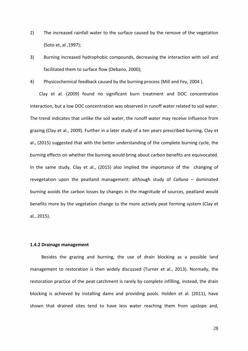
2) The increased rainfall water to the surface caused by the remove of the vegetation

(Soto et, al ,1997);

3) Burning increased hydrophobic compounds, decreasing the interaction with soil and

facilitated them to surface flow (Debano, 2000);

4) Physicochemical feedback caused by the burning process (Mill and Fey, 2004 ).

Clay et al. (2009) found no significant burn treatment and DOC concentration

interaction, but a low DOC concentration was observed in runoff water related to soil water.

The trend indicates that unlike the soil water, the runoff water may receive influence from

grazing (Clay et al., 2009). Further in a later study of a ten years prescribed burning, Clay et

al., (2015) suggested that with the better understanding of the complete burning cycle, the

burning effects on whether the burning would bring about carbon benefits are equivocated.

In the same study, Clay et al., (2015) also implied the importance of the changing of

revegetation upon the peatland management: although study of Calluna – dominated

burning avoids the carbon losses by changes in the magnitude of sources, peatland would

benefits more by the vegetation change to the more actively peat forming system (Clay et

al., 2015).

1.4.2 Drainage management

Besides the grazing and burning, the use of drain blocking as a possible land

management to restoration is then widely discussed (Turner et al., 2013). Normally, the

restoration practice of the peat catchment is rarely by complete infilling, instead, the drain

blocking is achieved by installing dams and providing pools. Holden et al. (2011), have

shown that drained sites tend to have less water reaching them from upslope and,

29

therefore, the water table maybe lower on one side of the drain than the other. Hence drain

blocking can be claimed to solve this problem by supplying a pool of water that seeps

through the hill slope, therefore, drain blocking might be a possible pathway to control the

DOC release.

However, the efficiency of drain blocking is doubted by the results of some studies

which show a conflicting trend. Daniels et al. (2008) and Holden and Burt (2002) showed the

evidence that the raised water table may increase the flashiness which may indicate

efficiency of drain blocking. This findings is then challenged by Armstrong et al. (2010) who

found a decrease in DOC and discharge upon drain blocking. The two findings are indeed

conflicting and require further study for explanation. Possible reasons are listed by Wilson et

al. (2011), whom indicated that the conflicting results may have been caused by the

variations between the study sites, but these differences also require further investigation.

The study of Holden et al. (2011) showed that the blocked drains appeared to have

hydrological functions moving towards the level of intact drains, however, this is varied

owing to spatial and physical impacts. In the long term, the dynamics of these restored

peatlands are doubted, and even if the hydrological function is restored, the timescale is

much longer than anticipated by most restoration programmes (Holden et al., 2011). Wilson

et al. (2011) and Tuner et al. (2013) did a study on the DOC concentration trend after the

drain blocking; the effects were somehow minimal and limited. Wilson et al. (2011)

estimated the DOC concentration for two study sites: an unblocked drain (A) and a post-

blocked drain (B). The results showed a decline in DOC concentration after the drain

blocking (Wilson et al., 2011), matching the study of Gibson et al. (2009) who also showed

that changes in DOC concentration are probably small in magnitude after blocking. The

increase of DOC might be because of the sharp decline of flow rate and yield decline after

30

drain blocking (Wilson et al., 2011). On the other hand, Armstrong et al. (2010) showed that

a blocked drain had a higher DOC concentration with higher flows than those of unblocked

drains. Wilson et al. (2010) indicated the importance of the discharge rates in determining

overall organic carbon losses. The hypothesis that water table depth would control the DOC

behaviour has been tested by Turner et al. (2013) and results for DOC export showed that

the reduction in export was only 9.2% at zero-order drains and 2.2% at first-order drains, i.e.

the effect of drain blocking was lost at larger scales. There are potentially several reasons

for the small effect of drain blocking. The bypass flow around the blockage was observed to

add high DOC concentration to the runoff flows down the drain. The alternative hypothesis

was proposed by Freeman et al. (2001), the so-called ‘enzyme latch ‘mechanism’, by which

hydrolase enzymes increase the DOC production and this process will not stop right after

the restoration of the water table. However, Wilson et al. (2011) has showed a reduction of

DOC from deeper peat simultaneous with drain-blocking, but failed to found evidence to

support the ‘enzyme latch’ mechanism. Furthermore, the effect which caused by the change

of water table depth observed by Tuner et al. (2013) was only 1 cm. The results of Tuner et

al. (2013) also matched the result of the study of Gibson et al. (2009), which showed that

the drain blocking did decrease the export of DOC but only achieved by decreasing water

yield. What’s more, the observed decrease in absorbance and DOC concentration could only

explain 1% of variation in their data. Thus, the use of drain blocking to control the DOC

release is an equivocal factor and needs further observation.

The changes of hydrological regime associated with drainage management are likely

to alter runoff response from peatland (Ballard et al., 2012). The hydrological regime

changes of peatland, which cause potential inimical changes of peatland runoff and raises

the chances of erosion have been widely discussed (Worrall et al., 2006, Holden et al.,

31

2007). Observations suggest that increased temperature and changes in rainfall patterns

could leads to the production of DOC (Worrall et al., 2004, Clark et al., 2007). Unlike the

widely discussed drain blocking effects on the DOC export, the drain blocking impact on

peak flows has not been conclusively covered by research to date. The concentration of DOC

has been associated with discharge and frequently correlated to storm events.(Austnes et

al., 2009). Several studies has illustrated the correlation between DOC export and flow path

changes in the organic mineral soil (Dawson et al., 2002; Soulsby et al., 2003). The

concentration changes of DOC has been associated with the flow path changes where the

higher DOC concentration from increased lateral flow through the upper horizon compared

to the lower horizon were exported with peak flow in organomineral soil (Worrall et al.,

2003). Peat and organic mineral soil differ in terms of profile and hydrological behaviour,

and therefore DOC dynamics would also differ in response of the storm events. In peatland,

the carbon stored in lower horizon (catotelm) is hydrologically disconnected from the

stream (Billett et al., 2006, Clark et al., 2007) where the base flow of the stream is

characterised as alkaline poor ground water (Worrall et al., 2002) and hydrologically

connected between peat and the mineral soil. When the water table rise during the peak

flow event, the upper horizon (acrotelm) flow with DOC rich soil water would raise the

stream DOC concentration (Worrall et al., 2002, Clark et al., 2008). Holden et al. (2011)

further indicated that DOC export is controlled by either saturated overland flow and

macropore flow of peat matrix, or direct rainfall dilution during the peak flow events. The

drainage area were correlated with peak flow event water contribution to storm (Pearce et

al., 1990; Brown et al., 1999).

32

1.4.3. Revegetation

The main effects of peat land management e.g. peatland drainage and burning includes

changes of water table, hydrology, water quality, sediment flows and vegetation (Bellamy et

al., 2012). The peat land restoration in UK is typically carried out by drain blocking in which

water table been raised (Turner et al., 2013) and in turn the blocking also encourages the

growth of peat formatting plant species (i.e. Sphagnum) (Holden et al., 2007; Peacock et al.,

2013). Restoration by drain blocking often helps to reestablish the vegetation. The

pioneering plant species such as Sphagnum often are indicative to the changes of species’

associated with improved fluvial carbon balance. In particular the recolonization of such

pioneer species are dominant and reestablished faster than the original species that

covered peat (Palmer et al., 2001; Robroek et al., 2010). The impact of the revegetation on

DOC export is highlighted as Parry et al. (2014) demonstrated that surface roughness may

play a more dominant role in terms of peak flow events. The transition from the bare peat

to vegetated peat would yield greater storm flow changes in rivers than blocked drains.

Thus, the revegetation would initially decrease the overflow and decreases the DOC export.

However, other studies (Robroek et al., 2010) indicate although the particulate organic

carbon (POC) of runoff water from peat land were recorded as having been stabilized

through the revegetation, DOC concentration and vegetation were found to be uncorrelated

to each other following the drain blocking (Bellamy et al., 2012; Kopeć et al., 2013; Peacock

et al., 2013). Unlike drain blocking, other land management such as burning strongly

effected the vegetation and often leads to significant changes in carbon cycle and hydrology

(Brown et al., 2015). The vegetation affects soil water balance through growth dynamic,

transpiration and interception. The removal of vegetation would elicit the chance of a runoff

event and thus introduce more DOC to the stream water (Robroek et al., 2010; Kopeć et al.,

33

2013). Further, vegetation removal with fire can significant alter the energy balance duo to

the exposure of more bare peat to solar radiation and therefore leads to the changes of soil

thermal regimes and thus leads to changes in carbon cycling, often with simultaneous

increased DOC concentration (Kettridge et al., 2012; Brown et al., 2015). The revegetation

with improving of self-regulated acrotelm by retaining high moisture level beneath the plant

canopies would lead to the substantially increased stability of the DOC production from the

peat (Ballard et al., 2011). Most studies are focused on the vegetation communities’

changes following peatland restoration (Brown et al., 2015); the relationship between

vegetation and ground water table (Kopeć et al., 2013). There is little in the literature about

revegetation impacts on DOC export followed by burning apart from Qassim et al. (2014).

The study (Qassim et al., 2014) looked through 5 years field study of the burned and

revegetated site in comparison of both a bare peat control and vegetated none –restored

control. The result of this revegetation study found a significant import of DOC in the soil

pore water of revegetated site in comparison to the bare peat and vegetated site and no

significant difference between soil pore water DOC concentration and runoff DOC

contortion. Qassim et al. (2014) also highlighted the possible drawdown of DOC export in

the runoff with the water table restoration alongside the vegetation. Therefore, further

study of revegetation effects on DOC runoff should be considered.

1.5 Bank filtration

Besides the possible land managements listed above for carbon release, other

possible hypotheses for prevention of DOC release might be considered. Bank filtration, for

instance, is widely used as a efficient water treatment both in Europe and United States

(Grunheid et al., 2005). In this process, the primary aim is to remove the pathogenic

34

microbes from the raw water, but also biodegradation processes would initially remove

turbidity and DOC (Grunheid et al., 2005). Therefore, bank filtration could be used as a

possible management to remove DOC. However, it should be noted that there are big

difference between how Europe and North American have reportedly used bank filtration

which initially might arise because of the designed retention time. In Europe, the retention

times are mostly designed for several weeks or even months according to the straight

demand for the drinking water whereas, in North America the retention time is only ranging

from several hours to days, at most a few weeks. As the DOC removal is mostly based on the

biodegradation process of bank filtration, the redox condition is then highlighted as its

control and the need for changing retention time (Grunheid et al., 2005). This is also

supported by the research of the Kim et al. (1997) who indicated no significant differences

between absorbed DOC in winter and summer and the percentage of biodegradable DOC

was higher in the winter than in summer probably due to active biodegradation in the

reservoir in summer. Furthermore, zonation was not effective to change the molecular

weight of organic substance, but could enhance biodegradability of DOC and reduce

absorbance in UV 260nm. It should be noted that even through the bank filtration could

decrease the DOC level of stream water, there is a potential danger to introduce other

contaminated compounds to the water sample, such as the increasing the dissolved iron by

the degradation through aquifers (Kim et al., 1997). Either natural or induced through the

river bed by pumping from a system of connected lateral or vertical wells, riverbed

clogging’s beneficial effect on promoting the biogeochemical degradation of contaminants

and its disadvantage on the reducing the hydrological conductivity of the infiltration zone

(Hiscock and Grischek, 2002) were noticed. Mostly, these pump locations could be set near

to the riparian zone near the drains (Fiebig et al., 1990). The possible effects of the riparian

35

zone on the DOC releasing is then discussed, with again some studies showing that the

riparian zone can contribute substantial amounts of DOC to a stream ecosystem, and that

the stream bed must be a key area of chemical reactivity where much of this material is

initially processed. As the delivery of DOC to the stream bed will depends on the hydrology

of the riparian zone, knowledge of this is an essential prerequisite to modelling the transfer

of organic material from a catchment to a stream. It is indeed unclear how the effects of the

hydrology process would also potentially 1) increase the DOC instead of the suspended 2)

sometimes decreasing when building bank filtration on riparian zone and pump water from

stream through aquifer to dip wells. Thus, it is necessary to undertake further study of the

bank filtration of the riparian zone.

1.6 Aim and object

This introduction chapter has illustrated the importance of the management of DOC upon

the UK upland peat with is impacts on both the carbon cycle and water treatment. A series

of heated researches has been interested in the effect of land management upon the

peatland (Gibson et al., 2010; Worrall et al., 2014), especially the impact land management

may have on the DOC. Studies of the burning and grazing of peat land carbon management

(Worrall et al., 2008; Clay et al., 2015) found both the burning and grazing were equivocal

on the effects which benefits the carbon sink. Therefore, this thesis will focus on the work

of DOC management through land management such as drain blocking, revegetation and a

pilot study of potential use of bank filtration as tools of such management. Despite the

effects such as those described by Turner et al. (2013), which previously contributed on the

drain blocking effects on DOC management, the impacts of peak flow events on the such

management have rarely been discussed. This present work also included a chapter of peak

36

flow events upon drain blocking effects in which would hopefully enhance a better

understanding of the drain blocking as a management of DOC in upland peat.

This can be broken down to series of specific objectives:

1) Measurement of the DOC concentration and budget on a series of nested and

blocked catchments. Chapter 2 will be dedicated on such aim by assessing a five

year long field observation on drain blocking in Northern England. By comparing the

DOC concentration and export from both blocked and unblocked catchments in the

study site over the periods before and after the blocking applied to site, decreased

DOC exports and concentrations would be expected duo to blocking.

2) Access the blocking effects upon the peak flow events in upland peat. Following the

findings and discussion on drain blocking in chapter 2, Chapter 3 will be focused on

the drain blocking impacts on DOC during the peak flow events. If the drain blocking

was proved to be an efficient practice of controlling the DOC releasing from peat

soil during the study period in Chapter 2, then drain blocking would be also

expected to be an efficient practice during the peak flow events during study

periods. It is crucial to assess the efficiency of drain blocking during peak flow

events, as the most DOC exports from soil to water were occurred during peak flow

events.

37

3) Assess the impact of revegetation on DOC changes in upland peat streams. As a

common management in Northern England peat, cool burning was widely applied

(Clay et al., 2009). Chapter 4 will assess how revegetation affects DOC release to

stream runoff after cool burning by comparing a revegetated catchment and a bare

catchment site. Revegetated catchment compare to bare catchment would

expected a much more stable water table and thus may lead to an also more stable

and lower DOC export over the study periods.

4) Assess bank filtration as an alternative approach to the management of high DOC

concentrations. A pilot study was performed on the side of the major field

observations to assess alternative management to drawdown runoff DOC in chapter

5. The assessed management is bank filtration, where was successfully applied in

Germany as water treatment and proved to decrease the runoff DOC (Grünheid et

al., 2005). By conducting a column study to mimic the filtration process using river

bank soils from river wear, filtrated water DOC would use to compare with the

runoff water DOC to assess whether the practice is suitable for river wear or not.

38

Chapter 2 Drain blocking

2.1. Introduction

This study was designed to evaluate the potential positive influence of drain blocking

on dissolved organic carbon (DOC) releasing from peat. There are several reasons for

concern over DOC with respect to water quality that was discussed in detail in chapter 1.

These can be summarised as:

1) Peatlands in the UK could be changing from a carbon reservoir to carbon sources

(Freeman et al., 2001), and an important component of the carbon release in UK is via

aquatic flux (Dinsmore et al., 2010). The aquatic flux of carbon from peat soils is commonly

related to changes in the depth to the water table. Dissolved organic carbon (DOC) flux is

one of the most important pathways of aquatic carbon release. At the same time, DOC is

also generally considered to be the largest contributor to aquatic carbon among the aquatic

components (Limpens et al., 2008).

2) The removal of DOC from water is a major water treatment issue. Unsuccessful

removal of DOC may cause aesthetic problems in drinking water supply, which is a key part

of the disinfection process (Wilson et al., 2011), and breech environmental standards (such

as EU Water Framework Directive, 2000/60/EC).

There are several possible hypothesises to explain the observed increase in DOC

release from peat soils that have been outlined previously (Chapter 1). Among all of the

explanations it is clear that water table fluctuation is seen as an important factor, which

highlighted the importance of managing a stable water table in control of DOC releasing

from peatland (Worrall et al., 2008; Holden et al., 2011).Several common land management

39

practices could influence DOC release from peat bogs, these include: grazing, burning and

drainage. These management practises would initially cause the fluctuation of the water

table which could couple with climate change to increase the release of DOC. Normally, the

water table depth in intact peatland is close to the surface during most parts of the year and

water table fluctuations are generally limited (Holden et al., 2011). However, the peatlands

of the UK are usually drained in response to resource demand, including 1) enhanced

agriculture demand in marginal areas of productivity; 2) afforestation; 3) horticulture and

energy production; 4) prevention of flood risk (Holden et al., 2011). Therefore, the

drawdown of the water table in drained blanket peat was observed throughout the UK

(Holden et al., 2011). However the observed results usually fail to find significant impact

between the drain and drawing down of the water table. (Stewart et al., 1991). As listed in

chapter 1, the failure of finding impacts between DOC and water table might be caused by

the site difference (Holden et al., 2003) or slope effects of the study site (Armstrong et al.,

2009).

In case of providing a stable water table, which initially may control the DOC release,

the uses of drain blocking as a possible land management for peatland restoration is widely

discussed (Turner et al., 2013). Normally, the restoration practice is rarely achieved by

completing infilling, instead, the drain blocking is achieved by installing dams and providing

pools. Holden et al. (2011), have shown that drained sites tend to have less water reaching

them from upslope and, therefore, the water table maybe lower on one side of the drain

than the other. Hence, the drain blocking might solve this problem by supplying a pool of

water that seeps through the hill slope. Therefore, drain blocking alters depth to water table

and could alter flow paths through the peat thus changing DOC release.

40

In this chapter, a year and half of stream water samples from post-blocking periods in

the study site, which we collected by the author and pre-blocking samples by Turner et al.,

(2013) to access a total three and half years drain blocking project conducted in northern

English upland. The aim of the project is to test whether the blocking effects the DOC export

and concentration changes and whether the blocking effects upon DOC would be effected

by different catchment scales.

2.2 Methodology

The approach of this study was to test the effect of drain blocking on the release of DOC

from peatland in the UK. In the study, two sets of paired catchments have been observed

for a year prior to any blocking, one set of drains was then blocked and the other left open,

both the open and blocked set were then monitored for three subsequent years. In each set

of drains there were two zero-order drains and a first-order drain, the zero-order drains

both feeding into the first order drain in each set. One of paired sets of catchments was

blocked as a treatment, while the other set remained unblocked as a control. Therefore, the

study allows comparison assessments in parallel controls of two scales of catchments during

several years. At the end of this period of monitoring a tracer experiment was conducted.

2.2.1 Study site

The study location was located on Cronkley Fell, an area of moor used for grouse shooting

and sheep grazing. The area was managed using rotational burning (Turner et al., 2013).

The six catchments share a common watershed and were divided into two sets of nested

41

catchments: the first set catchment is left unblocked through the whole study as the control

(National grid reference NY 83140 27284, Figure 2.1) at an altitude of 520 m above sea level;

the second set, which were blocked after one year using peat dams, were used as

experimental catchment, where located at an altitude of 570 m above sea level (National

grid reference NY83800 26996). The underlying geology of the catchments is a succession of

limestones of the Great Scar Limestone group. The vegetation of the catchments is

dominated by Eriophorum spp. (cotton grass), Calluna vulgaris (heather) and Sphagnum spp.

(moss).

Figure 2.1: Location of Monitoring Sites in Upper Teesdale (Turner, 2012).

42

Figure 2.2: Blocked drain in Cronkley Fell looking, north west to the Cowgreen Reservoir, October 2010

Within the context of two large catchments, individual ones can be monitored. For the

control set, first orders drain (CR3) and zero-order drains (CR1 and CR2) were monitored.

The actual scale of each three drains was: 0.230 km2 on CR1; 0.215 km2 on CR2; 0.750 km2

on CR3 (Figure 2.2 and Figure 2.3).

The experimental set of catchments follows a similar pattern to the control set, which

also had two zero-order catchments (CR5 and CR6), and a first-order catchment (CR4).

However, CR5 runs parallel to the rest of the site rather than flowing directly into CR4. The

topographic characters of CR5 are with a small cross-sectional area and lack of feeder drains

which means that CR5 has the typical characteristics of a zero-order drain. The other zero-

43

order drain (CR6) flows directly into CR4. In this set, CR4 has a catchments area of 0.715

km2, CR5 of 0.443 km2 and CR6 of 0.305 km2 (Figure 2.3).

Figure 2.3: Schematic diagram of monitoring site layout on Cronkley Fell (Turner, 2011)

KEY Monitoring site Flow direction

First order stream Soil water dip well network

Zero order stream Run off trap network

2.2.2 Sampling Program

To calculate the DOC export from each catchment, a detailed sampling program was

taken from 2011 to 2012, although data from the site were available form 2007 and

discussed in Turner et al. (2013). The author was involved in the last year and half of field

sampling and analyzed 1120 post blocking water sample, which are included in this chapter.

In the six study catchments, an automatic water sampler was positioned and took samples

of a frequency up to every 24 hours. It should be noticed that during later November to

early January the heavy snow made it impossible to get the study site.

44

Once the samples were collected, they were then transported to the laboratory. If the

samples could not be analyzed immediately they were frozen.

Figure 2.4 Display of V-Notch Weir and Autosampler in Cronkley, 2010.

2.2.3 Sampling Analysis

All samples collected from the field were analyzed for pH, conductivity, and absorbance.

The significant amount of samples from the study site also makes the measurement of DOC

concentration in every single sample impractical. Sample absorbance at 400 nm is typical for

the humic fraction of DOC (Thurman et al., 1985) and was thus used for the basic colour

reading. The E4:E6 ratio (Thurman et al., 1985), the ratio of absorbance at 465 nm and 665

nm, was used as a measure of DOC composition. Although there are some concerns of

inaccuracy relating water colour to DOC concentration (Wallage and Holden, 2010), a total

of 3945 samples were collected from the study site and 1125 samples collected from the

field were selected to present the actual range of flow, weather and seasonal conditions.

The selected samples were filtered through 0.45 μm filters and the DOC concentration

measured using the colorimetric method of Bartlett and Ross (1988). The method relies on

measuring the loss of colour by a Mn(III)-pyrophosphate complex as Mn(III) becomes

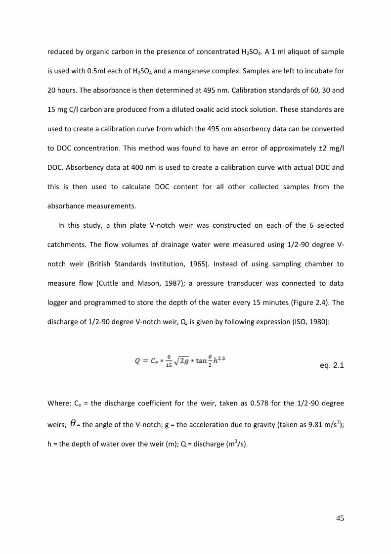
45

reduced by organic carbon in the presence of concentrated H2SO4. A 1 ml aliquot of sample

is used with 0.5ml each of H2SO4 and a manganese complex. Samples are left to incubate for

20 hours. The absorbance is then determined at 495 nm. Calibration standards of 60, 30 and

15 mg C/l carbon are produced from a diluted oxalic acid stock solution. These standards are

used to create a calibration curve from which the 495 nm absorbency data can be converted

to DOC concentration. This method was found to have an error of approximately ±2 mg/l

DOC. Absorbency data at 400 nm is used to create a calibration curve with actual DOC and

this is then used to calculate DOC content for all other collected samples from the

absorbance measurements.

In this study, a thin plate V-notch weir was constructed on each of the 6 selected

catchments. The flow volumes of drainage water were measured using 1/2-90 degree V-

notch weir (British Standards Institution, 1965). Instead of using sampling chamber to

measure flow (Cuttle and Mason, 1987); a pressure transducer was connected to data

logger and programmed to store the depth of the water every 15 minutes (Figure 2.4). The

discharge of 1/2-90 degree V-notch weir, Q, is given by following expression (ISO, 1980):

eq. 2.1

Where: Ce = the discharge coefficient for the weir, taken as 0.578 for the 1/2-90 degree

weirs; = the angle of the V-notch; g = the acceleration due to gravity (taken as 9.81 m/s2);

h = the depth of water over the weir (m); Q = discharge (m3/s).

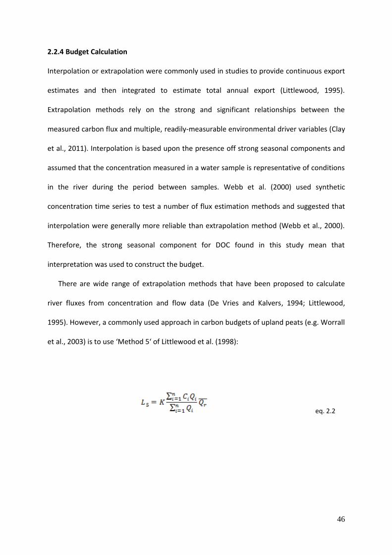
46

2.2.4 Budget Calculation

Interpolation or extrapolation were commonly used in studies to provide continuous export

estimates and then integrated to estimate total annual export (Littlewood, 1995).

Extrapolation methods rely on the strong and significant relationships between the

measured carbon flux and multiple, readily-measurable environmental driver variables (Clay

et al., 2011). Interpolation is based upon the presence off strong seasonal components and

assumed that the concentration measured in a water sample is representative of conditions

in the river during the period between samples. Webb et al. (2000) used synthetic

concentration time series to test a number of flux estimation methods and suggested that

interpolation were generally more reliable than extrapolation method (Webb et al., 2000).

Therefore, the strong seasonal component for DOC found in this study mean that

interpretation was used to construct the budget.

There are wide range of extrapolation methods that have been proposed to calculate

river fluxes from concentration and flow data (De Vries and Kalvers, 1994; Littlewood,

1995). However, a commonly used approach in carbon budgets of upland peats (e.g. Worrall

et al., 2003) is to use ‘Method 5‘ of Littlewood et al. (1998):

eq. 2.2

47

Where: Ci = instantaneous concentration; Qi = instantaneous flow; n = number of sampling

the record; rQ = the mean river discharge over the period; K = conversion factor for the

period of the record.

2.2.5 Statistical Analysis

This study was focused on the possible effects of drain blocking on DOC concentration

and export. Both the scale and drain blocking have been assessed in consideration of

impacts on DOC concentration and export. Further, water yield was considered as a

covariate in DOC export . Thus the analysis of variance (ANOVA) was used to analysis the

data here.

The factors considered in ANOVA were month of the year; site; drain-blocking status;

and scales of catchment. There were 12 levels on Month factors each represent a month in

a year. The site factor had 6 levels representing each monitoring site. The two sets of

catchments left blocked and unblocked which means 2 levels in drain-blocking status. Then,

the scales of drains had 2 levels, namely zero-order and first-order.

The existence of two sets of catchments makes it possible to consider the relative DOC

concentration. The relative DOC concentration is calculated as the ratio between post

blocking DOC concentration in both catchments. The ratios between the concentration of

blocked drains and unblocked drains were given in case of eliminating any effects of natural

variation on DOC concentration (for instance, the effects of year to year difference on DOC

values). The ratio values were considered as per the first analysis.

The analysis of DOC export considered the above factors again. What’s more, the water

yield from each drain in that month was also taken as covariates.

48

Post hoc comparisons between factor levels were made using Tukey test and the

magnitude of the effects of each significant factor and interaction were calculated using the

ω2 method (Vaughan and Corballis, 1969).

Besides the use of the ANOVA, the entire DOC exports dataset, between blocked and

unblocked catchments, was analyzed by double mass analysis. Double mass analysis uses

the curve between two cumulative values, x and y, and x is then plotted against y. The

curves allowed estimation of whether the variables had followed the same trends over the

course of the study period. Thus, any breaks in the slope of curve indicated a change in

trend for one of the variables (Searcy and Hardison, 1960). Double mass analysis was firstly

used to test the effects blocking has on the relationship between water yield and DOC

fluxes, and then on the relative accumulation of DOC exports between two catchments.

Whisker box plots were used across the entire thesis to give the visual illustration on the

subjected changes. An animated example was given in figure 2.5 to distributed different

sections of plots, where:

•A: upper whisker: represents the upper 25% of the distribution (excluding outliers)

•B: interquartile range box: middle 50% of the data

•C: median of the data.

•D: lower whisker represents the lower 25% of the distribution (excluding outliers)

49

yn

1.2

1.0

0.8

0.6

0.4

0.2

0.0

Blocked

Re

lati

ve

DO

C c

on

A

BC

D

Figure 2.5: illustration of whisker box plot.

50

2.3. Results

2.3.1 DOC concentration

From August 2007 to April 2012, 5260 samples were collected from Cronkley. Of these,

3945 of them were analysed directly for the DOC concentration using the method of Bartlett

and Ross (1988). For the rest of the samples the DOC concentration was calculated by

calibration curve between DOC concentration and absorbency at 400 nm. On both the

control and experimental catchment, DOC concentration changes were observed on

different scale and site (Figure 2.6, Figure 2.7 and Figure 2.8).

month

year

294116183105128

2012

2011

2011

2010

2010

2010

2009

2009

2008

2008

2007

2007

70

60

50

40

30

20Mo

nth

ly D

OC

co

nce

ntr

ati

on

(m

g C

g/

l) CR1

CR2

CR3

CR4

CR5

CR6

Variable

Figure 2.6: Time series of monthly DOC concentration of all catchments, where CR1- CR3 are control catchment; CR4-CR6 are experimental catchments. The access to study site was limited from June 2010 to April 2011, which left the gap in time series. The units of DOC concentrations are mg Carbon per g soil per liter sample.

51

Analysis of the monthly time series (Figure 2.6) for all the monitored sites shows a

strong seasonal cycle with the increase of DOC concentration during spring and summer. A

reversed relation between scale of drain and DOC concentration was observed throughout

the study periods. Differences between different scales of drains can be observed on the

time series (Figure 2.6). For instance, CR1 and CR3 in the control catchment (Black and

Green line in Figure 2.6); CR4 and CR6 in the experimental catchment (Blue and Pink line in

Figure 2.6) both observed an average of 22 mg C g/l increase from first order drain to zero

order drain.

CR3 20

11.3

CR3 20

10.3

CR3 20

09.3

CR3 20

08.3

CR2 20

11.3

CR2 20

10.3

CR2 20

09.3

CR2 20

08.3

CR1 20

11.3

CR1 20

10.3

CR1 20

09.3

CR1 20

08.3

80

70

60

50

40

30

20

10

DO

C c

on

ce

ntr

ati

on

(m

g C

g/

l)

Figure 2.7: The box plot of DOC concentration of control catchment on Cronkley Fell.

52

CR6 20

11.3

CR6 20

10.3

CR6 20

09.3

CR6 20

08.3

CR5 20

11.3

CR5 20

10.3

CR5 20

09.3

CR5 20

08.3

CR4 20

11.3

CR4 20

10.3

CR4 20

09.3

CR4 20

08.3

80

70

60

50

40

30

20

10

0

DO

C c

on

ce

ntr

ati

on

(m

g C

g/

l)

Figure 2.8: the box plot of DOC concentration of experimental catchment on Cronkley Fell.

The concentration of dissolved organic carbon in the control catchment increased with

increasing scale (i.e. CR1, CR2 - zero-order catchment, CR3 - first order catchment). A

notable concentration increase was observed between zero and first order drains (Figure

2.7), which might be the result of a combination of various processes. Firstly, natural DOC

degradation may have occurred as water moved down the catchment. However, earlier

studies of DOC degradation showed that these influences were small and cannot be the

main reason of DOC concentration decrease (Turner et al., 2013). Secondly, the DOC

concentration may dilute with increasing large amount of water from low DOC sources

being added into the system. It is suggested that with two reasons combined together, the

observed decrease of DOC concentration may be explained.

The DOC concentration of experiment catchment also showed a decrease with increasing

scale (Figure 2.8). Again this can be explained by a combination of the effects of dilution and

DOC degradation. A slight increase was observed in the drains after blocking. The median

53

DOC concentration change caused by blocking was an increase of between 3% and 23%

between zero and first order drains. The reason for this increase might be the effects of the

periods of monitoring, as concentrations may naturally fluctuate from year to year

independent of blocking status (Turner et al., 2013).

The ANOVA of DOC concentration data found that all these factors were significant at

least at the 95% probability and explain 42.5% of the original variance in the dataset. It

should be noticed that error term here explained 59.2% of the original variance. This high

proportion of the original variance due to the error term may not be just because of a

matter of measurement and sampling error, it could, for instance, represent some unknown

interaction between influential factors or covariates that could not be included in the

ANOVA. The lower P values in Turner et al. (2013) were all zero, which indicated the factors

involving in this study were more sensitive (Table 2.1) and this was probably due to the

additional data over the extra year since the study of Turner et al. (2013). The proportion of

variance showed that blocking explained a considerable proportion of the variance (10%),

which previous work didn’t find any significant influence for (Turner et al., 2013). This

significant change could be the result of various reasons; for instance, increased sample size

and time may increase the sensitivity of ANOVA. Among the three factors, the most

significant factor was scale, which explained 27% of variance. The interaction of scale and

month was significant, however it explained just 1% of the variance. Still, the presence of

significant interactions between month and scale showed different seasonal cycles for first

and zero-order streams.

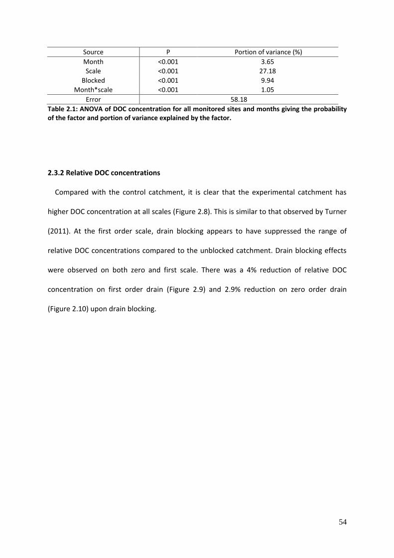
54

Source P Portion of variance (%)

Month <0.001 3.65

Scale <0.001 27.18

Blocked <0.001 9.94

Month*scale <0.001 1.05

Error 58.18

Table 2.1: ANOVA of DOC concentration for all monitored sites and months giving the probability of the factor and portion of variance explained by the factor.

2.3.2 Relative DOC concentrations

Compared with the control catchment, it is clear that the experimental catchment has

higher DOC concentration at all scales (Figure 2.8). This is similar to that observed by Turner

(2011). At the first order scale, drain blocking appears to have suppressed the range of

relative DOC concentrations compared to the unblocked catchment. Drain blocking effects

were observed on both zero and first scale. There was a 4% reduction of relative DOC

concentration on first order drain (Figure 2.9) and 2.9% reduction on zero order drain

(Figure 2.10) upon drain blocking.

55

first blockedFirst unblocked

1.50

1.25

1.00

0.75

0.50

rela

tiv

e D

OC

co

nce

ntr

ati

on

4%

Figure 2.9:The box plot of relative DOC concentration at first order catchment.

ZERO BLOCKEDZERO UNBLOCKED

0.95

0.90

0.85

0.80

0.75

0.70

0.65

0.60

rela

tiv

e D

OC

co

nce

ntr

ati

on

2.9%

Figure 2.10:The box plot of relative DOC concentration at zero order catchment.

56

ANOVA was performed on the relative DOC concentration factors, which included

the factors of blocking status, scale, and the interaction between blocking and scale (Table

2.2). Using relative DOC concentration eliminated the effect of seasonal differences and the

ANOVA showed that the scale factor was insignificant (Table 2.2). However, the interaction

between scale and blocking was found to be significant and explained 38.3% of the variance

in the dataset. This highlighted the possibility that blocking may be having an effect on DOC

concentration as scale changes. The majority of the variance in the dataset was explained by

blocking status: estimated at 42% of the original variance. The error term was about 20%,

which is a large decrease compared to the earlier analysis, which was 49.4% (Turner et al.,

2013). It also shows a reduction compared to the actual DOC concentration in this study and

shows the usefulness of the relative DOC which can eliminate a considerable proportion of

the unaccounted for natural variation. The ANOVA difference between DOC concentration

and relative DOC concentration here highlighted the reliability of relative values.

Source P Portion of variance (%)

Scale 0.212 0

Blocked 0.008 42.24

Scale*Blocked 0.01 38.83

Error 18.92

Table 2.2: ANOVA of relative DOC concentration for all monitored sites and months giving the probability of the factor/interaction and portion of variance explained by the factor.

57

2.3.3 DOC Export

The measurement of DOC export (g Carbon per m2) is the mass of DOC leaving the

observing catchments per unit area. The data were available from August 2007 to April

2012, which including both annual and monthly results.

There is an observed reduction in DOC export between the pre-blocking and post

blocking state. The annual DOC export reduction was recorded at all sites (Figure 2.11). The

reduction size varied with the change of site and scale. The result showed that reduction

was about 3% at zero order drain on control catchment and 0.65% on first order drain. This

reduction based on the control catchment reflected the natural year-to-year changes of

DOC export. Whereas the reduction observed on experimental catchments were 10% at

zero order drains and 2.56% at first order drain. This reflected the combination effects of

nature year-to-year variance and the effects of blocking on DOC export.

month

year

294116183105128

2012

2011

2011

2010

2010

2010

2009

2009

2008

2008

2007

2007

20

15

10

5

0

Mo

nth

ly D

OC

Exp

ort

CR1

CR2

CR3

CR4

CR5

CR6

Variable

Figure 2.11: Monthly DOC export time series for all sites.

(gC

/m2 )

58

ANOVA was performed with and without covariates. In this analysis, water yield was

used as a covariate. When the ANOVA was performed without water yield as a covariate,

month of year, scale, blocking statues and interaction of blocking and scale were found to

be significant (Table 2.3), with the majority of the variance being explained by the month of

the year and a increase rate of error term of 16.2%.

Source P Portion of variance (%)

Month <0.001 96.27

Scale 0.489 0

Blocked <0.001 3.73

Scale*Blocked 0.933 0

Error 0.002

Table 2.3: ANOVA of DOC export for all monitored sites and months giving the probability of the factor/interaction and portion of variance explained by the factor without covariant.

Source P Portion of variance (%)

Water Yield <0.001 88.21

Month <0.001 11.49

Scale 0.492 0.22

Blocked 0.286 0.04

Scale*Blocked 0.238 0.04

Error 8.79E-05

Table 2.4: ANOVA of DOC export for all monitored sites and months giving the probability of the factor/interaction and portion of variance explained by the factor.

It was found that when water yield was included in the analysis, water yield, site month

of the year, blocking status and the interaction of blocking and site are all significant and

together explained 89% of the original variance, i.e. the error term explained only 11% of

the original variance. Water yield, as a covariate, explained the majority of the variance in

the data set (88%, Table 2.4). However, the significance of water yield as covariance is that

export includes flow in its calculation and so it’s self-correlated. It should be noticed that

month factor also explained 11.4% of variance, which highlighted the seasonal change as an

influence on the DOC export. Besides the variance of water yield, it is rare to find that the

59

blocking (0.04%) and scale (0.22%) did not show a big influence on actual DOC export (Table

2.4).

Site Catchment/Scale TAE MAE Change in DOC Export

(%)

CR1 Control zero-order 78.54 76.21 -2.96

CR2 Control zero-order 77.97 75.62 -3.01

CR3 Control first-order 80.44 79.91 -0.65

CR4 Experimental first-order 61.57 59.97 -2.56

CR5 Experimental zero-order 72.7 65.81 -9.47

CR6 Experimental zero-order 62.56 55.02 -12.05

Table 2.5: The percentage change in total annual DOC export when the total annual DOC exports from the pre-blocking year is compared is compared to the mean annual total DOC export from the three post blocking years. Where: TAE=Total Annual DOC Export: Pre-blocking year (tC/km2), MAE=Mean Annual Total DOC Export: Post-blocking years (tC/km2).

A plot of DOC export against water yield for the zero order sites in the experimental

catchment demonstrates a clear reduction in the DOC export caused by the blocking (Figure

2.12). However, this decrease was not observed on the first order drain on the experimental

catchment (Figure 2.13). It is possible that the bypass flow around the zero order drain

blocks was adding additional water to first order drains, which initially suppressed DOC

export on this scale. The mixing effects of additional water source and any dilution effects

from alternatively sources of water would disrupt the expected linear relationship between

water yield and DOC export at this scale as seen in Figure 2.10. Also the combined effects

with additional water sources, dilution and DOC degradation might be acting at this larger

scale. The presence of any component of bypass flow or external water source will reduce

the efficiency of any blocking.

60

0.40.30.20.10.0

10

8

6

4

2

0

Water Yield

DO

C E

xp

ort

(g

C/

m2

/m

on

th)

Post-Blocking

Pre-Blocking

Figure 2.12: The correlation between water yield on DOC export at zero order scale for experimental catchment. Trend line: y=0.465+22.7x, R2=0.88

0.50.40.30.20.10.0

12

10

8

6

4

2

0

Water Yield

DO

C E

xp

ort

(g

C/

m2

/m

on

th)

Post-Blocking

Pre-Blocking

Figure 2.13: The correlation between water yield on DOC export at first order scale for experimental catchment. Trend line: y=0.057+21.2x, R2=0.78.

(m3/m2/month)

(m3/m2/month)

61

2.3.4 Relative DOC Export

The comparison of the DOC export between catchments (Figure 2.14) shows that at all

scales that the control catchment has higher DOC export than experimental catchment.. A

clear reduction in relative DOC export was observed between the blocked and unblocked

catchment at all scales, but the reduction was larger at the first order scale with 7%

reduction and 12% reduction at zero order drains. When ANOVA was performed on the

relative DOC export data; it was found that water yield, month of the year, scale, blocking

and interaction of scale and blocking were significant and in total explained 83.7% of the

original variance (Table 2.6). The error term explained 16.2% of variance. As above with the

DOC export, water yield still explained about 94% of the variance whereas the scale,

blocking and interaction between both explained the rest of the original variance in the

dataset. This comparison between water yield and other factors indicated how those

decreases in DOC export recorded post blocking are mainly controlled by reduction of water

yield than DOC concentration.

62

Source P Portion of variance (%)

Water Yield 0 94.65

Month 0.193 0.98

Scale 0.003 1.83

Blocking 0.009 2.34

Scale*Blocking 0.222 0.18

Error 0.00092

Table 2.6: ANOVA of relative DOC export for all monitored sites and months giving the probability of the factor/interaction and portion of variance explained by the factor.

first blockedfirst unblockedzero blockedzero unblocked

1.1

1.0

0.9

0.8

0.7

0.6

0.5

0.4

0.3

0.2

rela

tiv

e D

OC

exp

ort

Figure 2.14The box plot of relative DOC export at zero order and first order catchment.

63

2.3.5 Double Mass analysis

A linear trend is apparent in the double mass curve between cumulative monthly DOC flux

in both control and experimental catchments (Figure 2.15 and Figure 2.16). An instant

change on the slope of the double mass curve was observed on the zero order drains (CR5

and CR6) of the experimental catchment at the time of drain-blocking. The curve change is

clearly showed that a DOC change occurred post-blocking (Figure 2.15). Although the first

order drain (CR4) doesn’t show the instant break like others, it is possible to show a

continuing decrease on DOC flux with the increasing water flux in future observation (Figure

2.15). There is no slope break observed on the double mass curve for the control catchment

where no drain blocking happened (Figure 2.16). This excludes the possibility that the slope

break in the double mass curve for the experimental catchment was due to a common

change in both catchments.

Figure 2.15: Double Mass Curve for Cronkley Experimental Catchment. Blue Line represents the start of blocking. Where the Blue line shows the start of blocking.

(gC

)

(m3)

Blocking

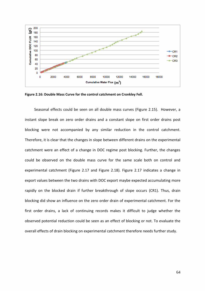
64

Figure 2.16: Double Mass Curve for the control catchment on Cronkley Fell.

Seasonal effects could be seen on all double mass curves (Figure 2.15). However, a

instant slope break on zero order drains and a constant slope on first order drains post

blocking were not accompanied by any similar reduction in the control catchment.

Therefore, it is clear that the changes in slope between different drains on the experimental

catchment were an effect of a change in DOC regime post blocking. Further, the changes

could be observed on the double mass curve for the same scale both on control and

experimental catchment (Figure 2.17 and Figure 2.18). Figure 2.17 indicates a change in

export values between the two drains with DOC export maybe expected accumulating more

rapidly on the blocked drain if further breakthrough of slope occurs (CR1). Thus, drain

blocking did show an influence on the zero order drain of experimental catchment. For the

first order drains, a lack of continuing records makes it difficult to judge whether the

observed potential reduction could be seen as an effect of blocking or not. To evaluate the

overall effects of drain blocking on experimental catchment therefore needs further study.

(gC

)

(m3)

65

Figure 2.17: Double Mass Curve for DOC export on zero order in both control and experimental catchment. CR1, control catchment; CR6, experimental catchment. The black trend line indicates the straight linear trend from which the curve is tending away. The data point represent cumulative monthly intervals. The blue line represents the start point of blocking.

Figure 2.18: Double Mass Curve for DOC export on first order in both control and experimental catchment. CR3, control catchment; CR4, experimental catchment. The curve does not tend away from the trend line post blocking. The data points represent cumulative monthly intervals. The blue line represents the start point of blocking.

(gC

) (g

C)

(gC/m2)

(gC/m2)

Blocking

Blocking

66

2.4 Discussion

Evaluation of DOC release from peat bog in Cronkley Fell was based on four years of

observation. Both actual and relative values were used to show the change of DOC behavior

in this peat bog. It was found that relative values, which could eliminate the natural year-to-

year variance, were more sensitive than actual values. The reduction of DOC concentration

and DOC export were observed on both first order and zero order drains, however, the size

of the reduction was only 2.2% on the zero order and 4 % on the first order drain.

At different scales, the reduction of DOC concentration was observed, but the drain

blocking effects were not as big as might be expected. A small fluctuation was observed

both on the control catchment and experimental catchment. The ANOVA suggested the

biggest contribution to this reduction is the natural seasonal change rather than blocking.

Use of relative rather than absolute values can eliminate the effects of year-to-year natural

changes effects on the DOC values. A reduction still exists on both catchments. It is

comparatively small at only 2.9% on zero order drains and 4% on first order drains. It also

should be noticed that with the increasing of the scale the DOC reduction is bigger. The

difference between DOC reductions at different scales indicates that the effects of drain

blocking may get bigger at larger scales. However, this difference with scale may not be a

result of drain blocking; it may be caused by the potential water sources that adding into the

first order drain. The large amount of extra water may increase the water table and

therefore cause the dilution of DOC concentration on first order drains. Apart from the scale

effects on the DOC concentration changes during study, the observed positive DOC

concentration decrease can be speculated to be duo to the DOC concentration being

strongly related to water table. This speculation assumes that if there is observed significant

water table changes, it would be expected to show as observed DOC concentration changes.

67

The controversial point is that there was not an observed significant water table change,

which may indicate other possible reasons that increase DOC export. For instance, the

potential water bypass sources, which were adding DOC to the study catchment

According to the observed water yield data in DOC export, it is also showed it is the

water table, instead of the blocking, explains the large part of variance of DOC export where

the water table explained 88.21% variances of ANOVA of DOC export and blocking factor

only explained 4% variances. It is clear that the DOC export followed the change in the

water yield rather than the drain blocking.

2.5 Conclusions

Drain blocking on Cronkley Fell based on four years observation from 2008 to 2012,

has shown that DOC concentration did decrease upon drain blocking. However, the effect

of drain-blocking was lower at larger catchment scales. Result of observations showed that

there is a 4% reduction of relative DOC concentration on first order drain and 2.9%

reduction on zero order drain; 12% reduction on zero order drain for relative DOC export

and 7% on first order drains. This clearly showed that the effect of drain blocking was

decreasing with increasing scale.

68

Chapter 3 Events analysis 3.1. Introductions

There are several reasons why the study of storm events is of increasing interest to

upland peat and hydrology research. First, the transportation of dissolved organic carbon

(DOC) from soil systems to the aquatic system remains an important part of the carbon

cycling. Numerous research studies have reported the increasing DOC concentration in

upland catchments draining peat soils (Worrall et al., 2004, Wilson et al., 2011) and the

majority of this DOC export is during storm events (Clark et al., 2008). Second, studies of

storm events give insight into the flowpaths and sources of DOC within the catchment

(Worrall et al., 2007, Austnes et al., 2009). During the hydrological peak, the DOC export is

controlled by either the dilution from direct rainfall or interactions with the peat matrix

(Holden et al. 2011). The interactions between different flowpaths can lead to variations in

the concentration and composition of DOC leaching to the surface water between and

during events. Besides the flow pathways, Pearce et al. (1990) found that event water

contributions to storm flow increased with increasing drainage area. Brown et al. (1999)

found peak runoff increased significantly with increasing catchment area, whereas the

event-water contributions at the hydrography peak decreased significantly with increasing

catchment area for all but the most intense rainfall events.

The mix of flowpath determines surface water chemistry during and after the peak flow

events (Brown et al. 1999). End-member mixing models of various kinds have been used to

understand the sources and pathways in catchments (Christophersen and Hooper, 1992).

Worrall et al. (2003) used two end-member mixing model to assess old versus new water

contributions to runoff in the peat catchment, however, three and four end-member

69

analysis have also been also used (Worrall et al. 2006). Further more, the interpretation

between the principal components analysis (PCA) and end-member analysis (EMMA ) has

been widely used in the study of peat-covered catchments (eg. Worrall et al., 2006). This

study used PCA to understand the composition and sources of events water between

managements in a peat-covered catchment.

As observed in the previous chapter, the concentration and flux of DOC observed as a

result of drain blocking will change with scale of catchment and the blocking may alter the

flowpaths operating during an event. For example, the blocking of drains could lead to

longer residence times in the catchment. Therefore, an event analysis was conducted to

assess different flowpaths. PCA and EMMA were conducted on the hydrological

characteristics of the events. The same analysis included a range of chemical parameters to

aid the investigation of the concentration changes during the events. ANOVA was used to

determine whether drain blocking had an effect during the events.

3.2. Methodology

Events recognition exploits the outputs of hydrological changes as well as changes in DOC

concentration and DOC flux in order to detect changes due to drain blocking. The analysis is

based on characterising individual flow events using a range of hydrological data and

including DOC flux and concentration changes over the subsequent days.

The approach of this study was to include non-events in the analysis, i.e. the event

analysis started with consideration of rainfall events and if they did not result in a

measurable runoff event then this was recorded as a non-event. The events analysis was

based on the data collection used in chapter 2, where three years drain blocking analysis

was conducted. The final data set considered one year pre-blocking data from January 1st,

70

2008 to February 28th, 2009 and two years post-blocking data Match 1st, 2009 to April 1st ,

2010.

Storm hydrographs for each flow gauge were plotted against rainfall, and standard

parameters were measured either from hydrograph or calculated from the time series.

The parameters were (Figure 3.1):

1. Rainfall characters

Each individual rain storm was described by the total rainfall of the day (mm), the rainfall

duration (hours),and peak rainfall intensity (mm/hour ).

2. Flow characters

The flow characteristics considered were: the flow lag time (hour), peak flow of the day

(m3/s), and the antecedent flow (m3/s). Therefore, the analysis gathered the information of

flow conditions of two days during a single event and linked the flow condition with next

day’s DOC concentration and flux changes.

3. Time since previous event

The time between events was included in the analysis whenever possible. However, due to

heavy snow conditions; changes in the fledging season and equipment failure, there are

gaps in the record which meant that it was not always possible to measure the actual time

between events.

71

Figure 3.1: Deconstruction of hydrograph for event analysis showing the characteristics considered.

Events analysis was also performed with the consideration of the DOC concentration

changes and DOC flux changes which were calculated from water samples before and after

the rainfall events. The DOC concentration changes and flux changes were calculated from

water samples taken from the autosampler in the field. As mentioned in earlier chapters,

the sampling was programed to take samples every 24 hours. That means the DOC

concentration were selected only 24 hours after the peak flow even through flow events

may last longer or shorter than this.

3.3 Statistical analysis

Analysis of variance (ANOVA) was used in two separate ways to assess the impact

that drain blocking had upon both the DOC concentration and DOC flux. Firstly, the DOC

concentration change from the every single events was considered along with the factors:

year, month, site, scale, and blocking statue. The Month factor has 12 levels, one for each

month of the year. The site had 6 levels one for each of the monitored catchments. The

scale factor had two levels, zero and first order. Even through the site differences would

explain more variance of data set, the scale factor was included in this analysis to minimize

m3/s

72

the difference of the actual site difference. The blocking had two levels: blocked and

unblocked. Along with the four main factors, the hydrological data including: rainfall total,

rainfall duration, peak rainfall intensity, flow lag time, peak flow, antecedent flow, and time

between events were used as covariates. The same analysis was repeated for change in the

DOC flux.

To negate effects of the natural variations in DOC from year to year, both the DOC

concentration change and DOC flux changes of a blocked drain in experimental catchment

were considered relative to the DOC concentration and DOC flux of an unblocked drain of

the same scale in the control catchment at the same time. Relative DOC was calculated by

the ratio of the monthly average DOC concentration or DOC flux of a blocked and unblocked

drain from the experimental and control catchments respectively. The relative DOC

concentration and flux changes were subject to ANOVA as above.

The event analysis included a large range of hydroclimatic characteristics and

responses and therefore a multivariate analysis was required to produce easily interpretable

results. Principal components analysis (PCA) is a multivariate analysis that allows data

described by multiple primary variables to be converted into the same number of principal

components, which are mutually orthogonal (Harrington et al., 2005). The principal

components combine variables from the original dataset and are calculated in the order of

decreasing proportion of the original variance explained. In doing so it is hoped that by

using PCA the number of components which need to be examined is fewer than the original

number of variables while also highlighting multiple associations and correlations between

the original set of variables. Therefore, PCA was employed here to look through the impact

of hydrological factors on DOC concentration and DOC flux of the flow events.

73

The variables used in PCA were: rainfall total (mm), rainfall duration (hour), peak

rainfall intensity (mm/hour), flow lag time (hour), peak flow ( m3/s), antecedent flow (m3/s),

and time between events (hour). The PCA was first performed with DOC concentration and

then applied to DOC flux. Because the variables have different units all data were converted

to standard normal distribution by using z-transform before analysis. The z-transform is:

𝑍 =(𝑋−𝜇)

𝜎 eq. 3.1

Where: x is a raw value to be standardized; μ is the mean of the population; and σ is the

standard deviation of the population. The quantity z represents the distance between the

raw score and the population mean in units of the standard deviation: z is negative when

the raw score is below the mean and positive when above.

To assess which of the principal components (PC) would be retained for assessment

the following rule was applied: Chatfield and Collins (1980) states that when analyzing a

correlation matrix from a PCA the sum of the eigenvalue is equal to the number of variables,

therefore components with eigenvalues less than 1 may be disregarded as they represent

less variance in the original data than a single variable. Therefore, in the events analysis

here, all PCs with eigenvalues greater than 1 were considered but the first PC with

eigenvalue less than 1 was also included.

Christophersen and Hooper (1992) discussed multi-end-member interpretation in

combination with principal components analysis to identify the source solutions from

potential groundwater mixtures. The end-member mixing approach was then widely used as

an efficient analysis to evaluate the ability of independently measured source compositions

74

of combined water sources (Worrall et. al., 2003). Christophersen and Hooper (1992) argued

that PCA can only be used to identify the number of end-members prior to using the EMMA

approach, however, Worrall et al. (2003) argued this assumption is only valid if the end-

members are independently measured. However, the PCA doesn’t presume the nature of

the end-members and the EMMA is dependent on the end-member composition and its

antecedent conditions (Soulsby et al., 1995). In this study the composition at the catchment

outlet and the antecedent characters such as antecedent rainfall and antecedent flow (see

illustration in Figure 3.1) are gathered over the same time period with the same frequency.

This means the end-member mixing analysis can be performed for each component and in

combination to understand the sources and controls on the composition of the events.

Furthermore, the scores on key principal components (PCs) were chosen for ANOVA. This

process is aimed to investigate if these PCs are significant influenced by the blocking. During

the ANOVA, scale, blocking status, and month were considered as the factors, whereas DOC

flux was considered as a covariate. The factors had the same levels as described above.

3.4. Result of DOC Concentration

During the three years of study, there were 2710 rainfall events recorded from six drains.

Among these 2710 events, there were 1626 rainfall events which could be matched with a

measurable flow event and 1080 events with no identical flow events. That means there

were 271 days out of three years which were under the peak flow conditions. However,

equipment problems meant that the automatic sampler only collected samples every 24

hours, therefore when DOC concentration or export were considered then only 756 out of

1626 events could be included for analysis. A detailed description of the analyzed rainfall

and flow events can be found in Table 3.1.

75

Descriptor control Experimental

max min max min

Total Rainfall (mm) 33.6 0.2 33.6 0.2

Rainfall durations (h) 28.8 0.2 28.8 0.2

Rainfall intensity (mm/h) 25.6 0.08 25.6 0.08

Flow lag time (h) 3 0.25 3 0.25

Peak flow (m3/s) 0.430733 1.12×10-8 0.700052 3.07×10-7

Antecedent flow (m3/s) 0.430733 1.12×10-8 0.700052 3.07×10-7

Table 3.1: Detailed description of recorded rainfall and flow events.

The antecedent flow as an estimated base flow of the events, showed no significant

change before and after blocking (Figure 3.2), however flow lag times were observed to

increase after blocking (Figure 3.4). The flow lag times could be influenced by the different

Figure 3.2: Box plots of antecedent flow of blocked and unblocked drains. The lower whiskers (low 25% of data) of blocked drain in both scales are too close to up boundary of interquartile box to shown in figure.

yn

0.06

0.05

0.04

0.03

0.02

0.01

0.00

Blocked?

An

tece

ed

en

t fl

ow

(m

3/

s)

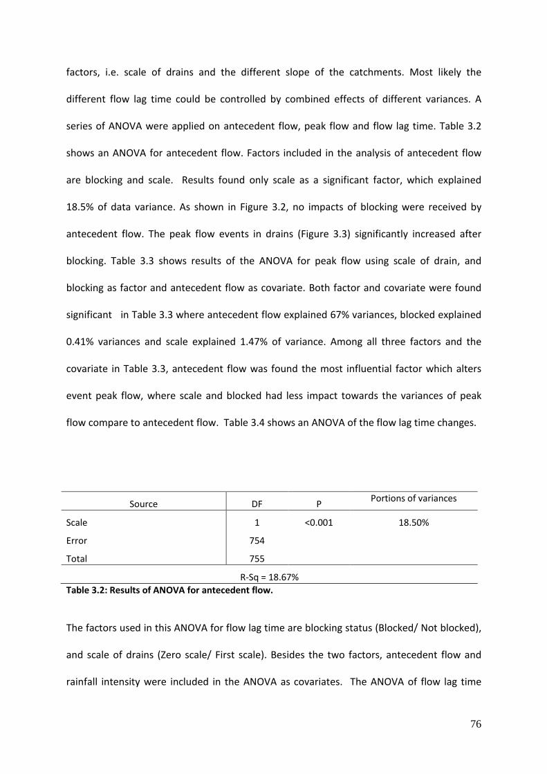
76

factors, i.e. scale of drains and the different slope of the catchments. Most likely the

different flow lag time could be controlled by combined effects of different variances. A

series of ANOVA were applied on antecedent flow, peak flow and flow lag time. Table 3.2

shows an ANOVA for antecedent flow. Factors included in the analysis of antecedent flow

are blocking and scale. Results found only scale as a significant factor, which explained

18.5% of data variance. As shown in Figure 3.2, no impacts of blocking were received by

antecedent flow. The peak flow events in drains (Figure 3.3) significantly increased after

blocking. Table 3.3 shows results of the ANOVA for peak flow using scale of drain, and

blocking as factor and antecedent flow as covariate. Both factor and covariate were found

significant in Table 3.3 where antecedent flow explained 67% variances, blocked explained

0.41% variances and scale explained 1.47% of variance. Among all three factors and the

covariate in Table 3.3, antecedent flow was found the most influential factor which alters

event peak flow, where scale and blocked had less impact towards the variances of peak

flow compare to antecedent flow. Table 3.4 shows an ANOVA of the flow lag time changes.

Source DF P Portions of variances

Scale 1 <0.001 18.50%

Error 754

Total 755

R-Sq = 18.67%

Table 3.2: Results of ANOVA for antecedent flow.

The factors used in this ANOVA for flow lag time are blocking status (Blocked/ Not blocked),

and scale of drains (Zero scale/ First scale). Besides the two factors, antecedent flow and

rainfall intensity were included in the ANOVA as covariates. The ANOVA of flow lag time

77

found blocking as most important factor by which explained 17.4 % of variance. Scale didn’t

show any significance in the analysis. Both the covariates were found as significant factor

with respect of explaining 4.35% of data variances by antecedent flow and 2.85% variances

of data by rain intensity. Changes of the events parameters may effects water runoff

reaction to the flow events after blocking been applied i.e. the increase of flow lag time

after blocking would in turn enhance the stream runoff.

Source DF P Portions of variances

Antecedent flow 1 <0.001 66.96%

Blocked? 1 <0.001 0.41%

Scale 1 <0.001 1.74%

Error 752 Total 755 R-Sq = 69.27%

Table 3.3: Results of ANOVA for peak flow.

Figure 3.3: plots for peak flow and antecedent flow measured from drains, prior and after blocking. The lower whiskers (low 25% of data) of blocked drain in both scales are too close to up boundary of interquartile box to shown in figure.

yn

0.12

0.10

0.08

0.06

0.04

0.02

0.00

Blocked?

Pe

ak f

low

(m

3/

s)

78

Source DF P Portions of variances

Rain Intensity (mm/hour) 1 0.001 2.86%

Antecedent flow 1 <0.001 4.35%

Blocked? 1 <0.001 17.24%

Error 435

Total 438

R-Sq = 25.01%

Table 3.4: Results of ANOVA for Flow lag time.

Figure 3.4: plots for flow lag time measured from drains, prior and after blocking.

yn

3.0

2.5

2.0

1.5

1.0

0.5

0.0

Blocked?

Flo

w la

g t

ime

(h

ou

r)

79

3.4.1. DOC concentration

The DOC concentration has been calculated on a total of 5960 samples. Of these

water samples only 756 could be associated with the flow events. Analysis of variance

(ANOVA) was performed on the DOC concentration data from Cronkley and covariates from

the next day hydrological behavior. In the ANOVA of 756 DOC concentration, the data set of

DOC concentration was replaced by its logged value so as to give a normal distribution (For

details of ANOVA see chapter 2). The following factors of ANOVA of DOC concentration

changes of events were found to be significant: month, site, and blocking status. The

combination of covariates and factors explained 50.78% of the original variance. Site was

the most important factor and explained 42.52% of the original variance in the dataset. The

month and blocking factors explained 4.2% and 3.29% of the original variance respectively.

Figure 3.5: DOC concentration changes before and after blocking.

yn

20

10

0

-10

-20

Blocked?

DO

C c

on

ce

ntr

ati

on

Ch

an

ge

s (

mg

g/

l)

80

The site and scale factors are correlated and so when the scale was used as a factor instead

of site, it was found that flow lag time, month, scale, blocking statue were significant and

explained 31.99% of variance. In this case scale was the most important factor and blocking

still only explained a small portion of the original variance (0.94%). The significant effect of

blocking was an average a decrease in DOC concentration changes of 0.8 mg g/l (Figure 3.5),

i.e. the change in DOC concentration across an event was smaller after blocking.

A clear difference between zero and first order drains can be observed for the control

catchments (Figure 3.6). The decrease in DOC concentration changes can be ascribed to the

greater dilution potential at scale and the longer residence time leading to greater DOC

losses via degradation processes.

Figure 3.6: DOC concentration changes in control catchment (where CR1 and CR2 are zero order drain and CR3 is first order drain).

CR3CR2CR1

15

10

5

0

-5

-10

-15

Site

DO

C c

on

ce

ntr

ati

on

Ch

an

ge

s (

mg

C g

/l)

81

The whisker plots of the experimental catchments show a similar pattern between the

DOC concentration changes between the different scales as observed for the control

catchments (Figure 3.7), where the zero order drains (CR5, CR6) show lower DOC

concentration changes than the first order drain (CR4) before blocking. Among two zero

order drains, CR6 showed relative smaller changes compare with CR4 and CR5 before and

after blocking, while CR5 showed a decrease after blocking. The different DOC concentration

changes could be due to a number of reasons, however the most likely is that different

setting of experimental catchment compared to the control catchment: unlike the control

catchment both zero order drains in the experimental catchment can be seen as two

parallel bypass drains to the first order drain, only CR6 can be seen as such a bypass drain in

the control catchment, CR5 is independent of CR4 (first order drain) and linked directly to a

shake hole. In this case, the significant decrease in DOC concentration changes after

blocking observed in CR4 can be explained by a combination of DOC concentration changes

by itself and an accumulation of DOC concentration changes from both CR6 and CR4. Vice

versa, because the independence of CR5 to CR4, therefore DOC concentration changes of

CR5 were not affected by the DOC concentration changes of CR4. Another possible reason

of the bigger DOC concentration changes in first order drains after blocking is that the bigger

scale drain might receive more influence from the blocking than smaller scale drains in the

experimental catchment. Blocking may have caused changes in flowpath during events that

caused water to go deeper into the soil and flush out higher DOC concentration soil water.

As mentioned earlier, the flow lag time is only dependent upon the blocking rather than

upon scale. After blocking both scales of drain would have had longer flow lag time that

triggered the events water exchanges with deeper soil water.

82

As the first order drain is bigger than the zero order drain, there would be more high

DOC concentration deeper soil water exported from depth in the soil, which resulted in the

greater decrease in the DOC concentration change across events for the larger scale drains

after blocking.

Figure 3.7: DOC concentration changes in experimental catchment.

Site

Blocked?

CR6CR5CR4

ynynyn

30

20

10

0

-10

-20

-30

DO

C c

on

ce

ntr

ati

on

Ch

an

ge

s (

mg

g/

l)

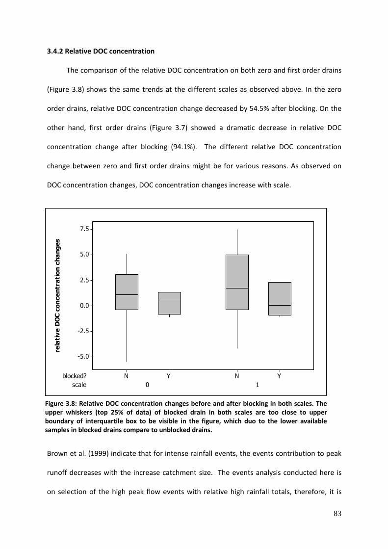
83

3.4.2 Relative DOC concentration

The comparison of the relative DOC concentration on both zero and first order drains

(Figure 3.8) shows the same trends at the different scales as observed above. In the zero

order drains, relative DOC concentration change decreased by 54.5% after blocking. On the

other hand, first order drains (Figure 3.7) showed a dramatic decrease in relative DOC

concentration change after blocking (94.1%). The different relative DOC concentration

change between zero and first order drains might be for various reasons. As observed on

DOC concentration changes, DOC concentration changes increase with scale.

Brown et al. (1999) indicate that for intense rainfall events, the events contribution to peak

runoff decreases with the increase catchment size. The events analysis conducted here is

on selection of the high peak flow events with relative high rainfall totals, therefore, it is

Figure 3.8: Relative DOC concentration changes before and after blocking in both scales. The upper whiskers (top 25% of data) of blocked drain in both scales are too close to upper boundary of interquartile box to be visible in the figure, which duo to the lower available samples in blocked drains compare to unblocked drains.

scale

blocked?

10

YNYN

7.5

5.0

2.5

0.0

-2.5

-5.0

rela

tiv

e D

OC

co

nce

ntr

ati

on

ch

an

ge

s

84

likely to suit the situation Brown et al. described. On the other hand, Brown et al .(1999)

linked the catchment size effects with the changes of flowpath, in which the pre-event

ground water was involved and they indicated a downstream increase in groundwater

compared to storm water. The greatest contribution of event water to storm flow was in the

smallest catchments where the near stream ground water reservoir was probably smaller.

Therefore, the higher order drain is more likely to see a dilution effect from the ground

water. The blocking of the higher order drain increases the flow lag time of the event, which

would lead to the mix of event water and pre event flow, this dilution impact would have a

much bigger impacts on bigger scale drains. The PCAs of the hydrological data and end-

member analysis of the different chemical tracers of the stream water were used to further

investigate this difference.

3.5. Principal components analysis of DOC Concentration

Four PCs were selected based upon the rule that eigenvalues > 1 and the first < 1, and

together they explained 76% of the original variance. Table 3.5 shows the loadings on the

PCs and that rainfall total, rainfall duration, time between events, flow lag time were all

unrelated to DOC concentration changes across all PCs. Traditionally, loadings of

approximately 0.5 were selected as important, however the analysis performed here

considered loadings bigger than 0.4 as important to include more possible variables. The

considered important loadings have been highlighted as red on the Table 2 – it should be

noted that there is no statistically-based rule that allows one to identify variables of

importance within a PC. The first two components together explained 48.2% of dataset

variance and PC1 represented 26.3% of the data variance. Normally, the first component

85

(PC1) is interpreted as a measure of overall variances and facilitates normalization of the

data variances (Worrall et al., 2003). In this events analysis, the z score standardized the

Absolute loading values bigger than 0.400 were considered as dominant loadings and marked red.

variables prior to the PCA, therefore PC1 here represents the actual changes in variables

rather than the difference between units.

In the four PCs, both PC1 and PC2 are mainly governed by changes in: rainfall total,

rainfall durations, peak flow, and antecedent flow. However, PC1 increases with all four of

these variables, while PC2 only increases with increased rainfall total and rainfall duration

but increased with decreasing peak flow and antecedent flow. PC1 seems to distribute

effects of the rainfall to the flow, i.e. increases in rainfall and increased antecedent flow lead

to increased peak flow. On the other hand, the PC2 shows negative loadings of antecedent

Table 3.5: Hydrological loadings of first four PCs.

Variable PC1 PC2 PC3 PC4

Z Rainfall Total (mm)_ 0.517 0.447 -0.052 -0.031

Z Rainfall Duration (hours)_ 0.524 0.426 0.120 -0.050

Z Rainfall Intensity (mm/hour)_ -0.057 0.079 -0.750 0.018

Z Flow lag time 0.220 -0.193 0.547 0.106

Z Antecedent flow 0.411 -0.532 -0.129 -0.008

Z Peak flow 0.392 -0.534 -0.166 -0.133

Z Time between events -0.289 -0.075 0.276 -0.162

Z DOC concentration changes -0.029 0.034 0.019 -0.970

Eigenvalue 2.1077 1.7514 1.1592 1.0128

Proportion 0.263 0.219 0.145 0.127

Cumulative 0.263 0.482 0.627 0.754

86

flow, peak flow and positive loading of rainfall total and rainfall duration. In this case, even

though the total rainfall and rain durations were getting bigger, the peak flow was still

decreasing. The decreased peak flow here might simply be due to the decreased antecedent

flow. Other possibilities include that this PC represents rainfall event which with high rainfall

total, high rainfall duration but low rainfall intensities, and therefore, peak flow could be

low during such long rainfall periods. Besides the above hypothesizes, Holden et al. (2008)

pointed out the existence of the peat pipes, which are common features of peat land

(Holden et al., 2002) may provide the event water with an additional flow path through the

sub soil that leads to the decreasing of the peak flow. The hypotheses given here maybe PC2

may represent a combination of potential flow path effects and low rain intensity effects

upon the peak flow. Therefore, PC2 here is used as an interpretation of counter factor

besides PC1 which represent the effects of rainfall.

The PC2, PC3 are dominated by positive loadings for flow lag time and negative loadings

of rainfall intensity. Loadings of PC3 suggest relationship between decreasing rain intensity

and increasing flow lag time. Loadings of PC4 show negative loadings of DOC concentration

changes, which make PC4 represent the factor of the DOC concentration changes during the

events.

Four individual components were divided to several groups to test the relationship

between hydrological factors and DOC concentration changes during the events. PC1 and

PC2 were first grouped together as both them shared the same important loadings through

each of them represent different movement of the event water. PC3 is then joined

separately to PC1 and PC2 as PC3 illustrate a periods of time between events that may show

different influences on different event water movements. Lastly, PC4 was considered with

PC1 and with PC2 to test the DOC concentration changes on two types of event water

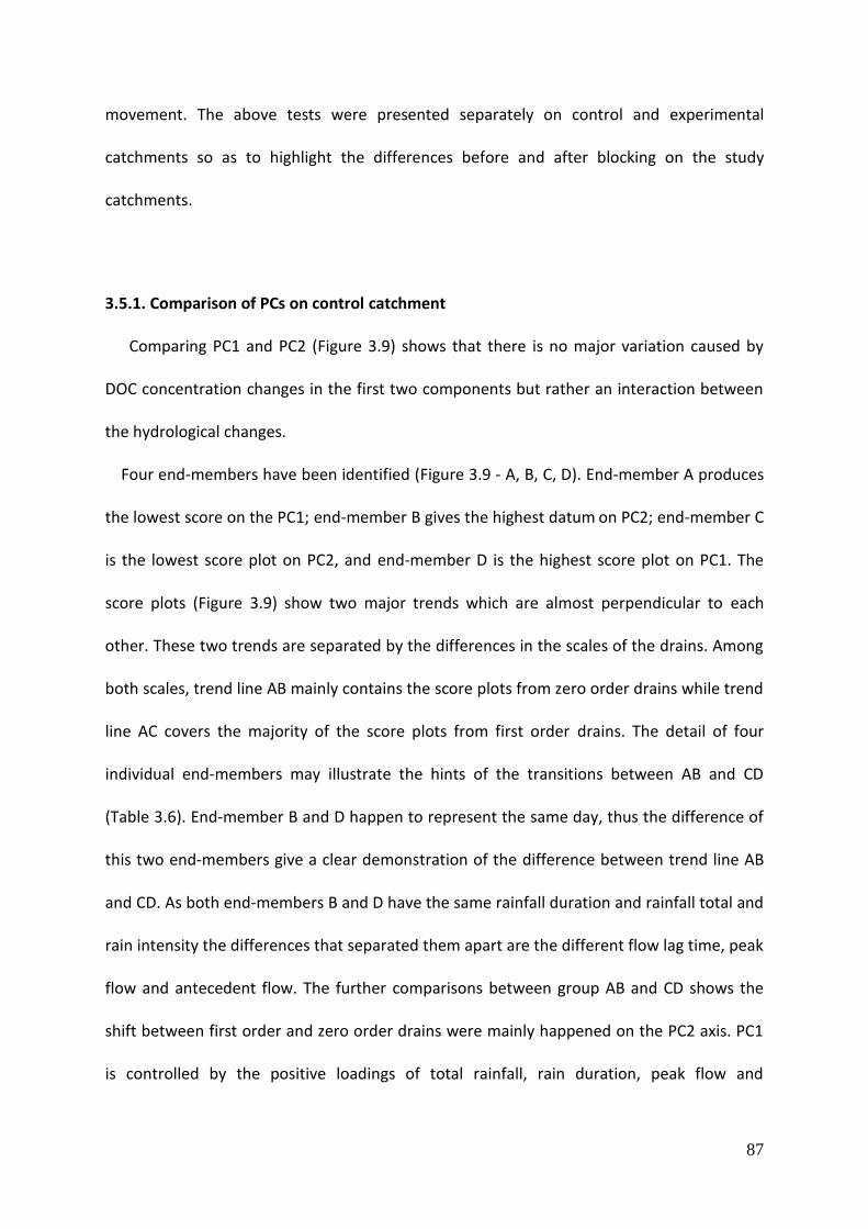
87

movement. The above tests were presented separately on control and experimental

catchments so as to highlight the differences before and after blocking on the study

catchments.

3.5.1. Comparison of PCs on control catchment

Comparing PC1 and PC2 (Figure 3.9) shows that there is no major variation caused by

DOC concentration changes in the first two components but rather an interaction between

the hydrological changes.

Four end-members have been identified (Figure 3.9 - A, B, C, D). End-member A produces

the lowest score on the PC1; end-member B gives the highest datum on PC2; end-member C

is the lowest score plot on PC2, and end-member D is the highest score plot on PC1. The

score plots (Figure 3.9) show two major trends which are almost perpendicular to each

other. These two trends are separated by the differences in the scales of the drains. Among

both scales, trend line AB mainly contains the score plots from zero order drains while trend

line AC covers the majority of the score plots from first order drains. The detail of four

individual end-members may illustrate the hints of the transitions between AB and CD

(Table 3.6). End-member B and D happen to represent the same day, thus the difference of

this two end-members give a clear demonstration of the difference between trend line AB

and CD. As both end-members B and D have the same rainfall duration and rainfall total and

rain intensity the differences that separated them apart are the different flow lag time, peak

flow and antecedent flow. The further comparisons between group AB and CD shows the

shift between first order and zero order drains were mainly happened on the PC2 axis. PC1

is controlled by the positive loadings of total rainfall, rain duration, peak flow and

88

antecedent flow. As mentioned earlier PC1 represents a hydrological relationship that the

flow would increase with increasing rainfall. Therefore, end-member A represents the

events that have low flow conditions and low rainfalls. From Table 1, PC2 represents the

condition that as rain fall increases, the antecedent flow and peak flow are still decreasing.

This may suggest that the base flow is not dependent on the current rainfall. Thus, end-

member B shows the events with the low peak flow and antecedent flow but with the high

rainfall total and rain duration.

The Line AB shows that the zero order drains were controlled by the events under the

increasing rainfall, low peak flow with low antecedent flow. On the contrary, end-member C

has the lowest score on PC 2 which has negative loading of peak flow, antecedent flow and

positive loadings of rainfall total and rainfall duration. Therefore, trend line AC shows that

major transition between zero order to first order drain, however all the loadings were

increased from A to C. End-members B and D are easier to compare in this situation as they

sharing the same rainfall total and rainfall duration. Noticeable, the changes between B and

D were mainly by different flow lag time.

End-

member Date Site Scale RT RD RI FLT PF AntF

A 28/03/2008 CR1 0 0.2 0.2 1 1 0.0005 0.0005

B 04/08/2008 CR1 0 28.8 28.8 1 1.25 0.0005 0.0004

C 10/11/2008 CR3 1 0.6 0.25 2.4 2 0.3945 0.2672

D 04/08/2008 CR3 1 28.8 28.8 1 2 0.3247 0.2499

Table 3.6: Hydrological characters of the four end-members in control catchment.

Where RT: Rainfall total (mm); RD: Rain duration (hour); RI: Rain intensity (mm/hour); FLT: Flow lag time (hour); PF: Peak flow (m3/s), AntF: Antecedent flow (m3/s).

89

The difference between the two scales of drains is the different flow lag times: this

may indicate that there are other factors controlling the event flow rather than the ones

included in this PCA.

The same separation can be observed on the plots that PC2 against PC3 (Figure 3.10). As

mentioned before that PC2 is general interpreted as representative of influence of high

rainfall but low rainfall intensity events. PC3 is taken to represent time periods which the

time between events was getting longer and rain intensity was decreasing. In Figure 3.10,

there is a clear separation between zero order drains and first order drains on the axis of

PC2. In control catchment, majority of the events plot on the positive end of PC3. In other

words, during the long flow lag time and low rain intensity events periods, zero order drains

reflect more events with small peak flow and antecedent flow under bigger rainfall total and

rainfall duration; first order drain have the events with smaller rainfall total and rainfall

Figure 3.9: Score plot PC1 vs PC2 on control catchment.

86420-2

5.0

2.5

0.0

-2.5

-5.0

PC1

PC

2

CR1

CR2

CR3

Site

A

B

C

D

90

duration but bigger peak flow and antecedent flow. On Figure 3.10, two end-members were

identified. These two end-member represent the same day of the hydrological events C and

B in Figure 3.9. Their hydrological details were given by Table 3.7. In Table 3.7, it is clear that

the rise and fall of event flow were following the same trend of rainfall intensity and flow lag

time. When the flow lag time were decreased from C to B, peak flow and antecedent flow

also decreased despite that end-member B has bigger rainfall total and rain durations. It is

noticeable that in end-member C, the rainfall duration is much smaller than flow lag time

which means that by the time the rainfall stops, the steam is still receiving event water.

Figure 3.10: Score plot PC2 vs PC3 on control catchment.

5.02.50.0-2.5-5.0

2

1

0

-1

-2

-3

-4

-5

-6

-7

PC2

PC

3

CR1

CR2

CR3

Site

B

C

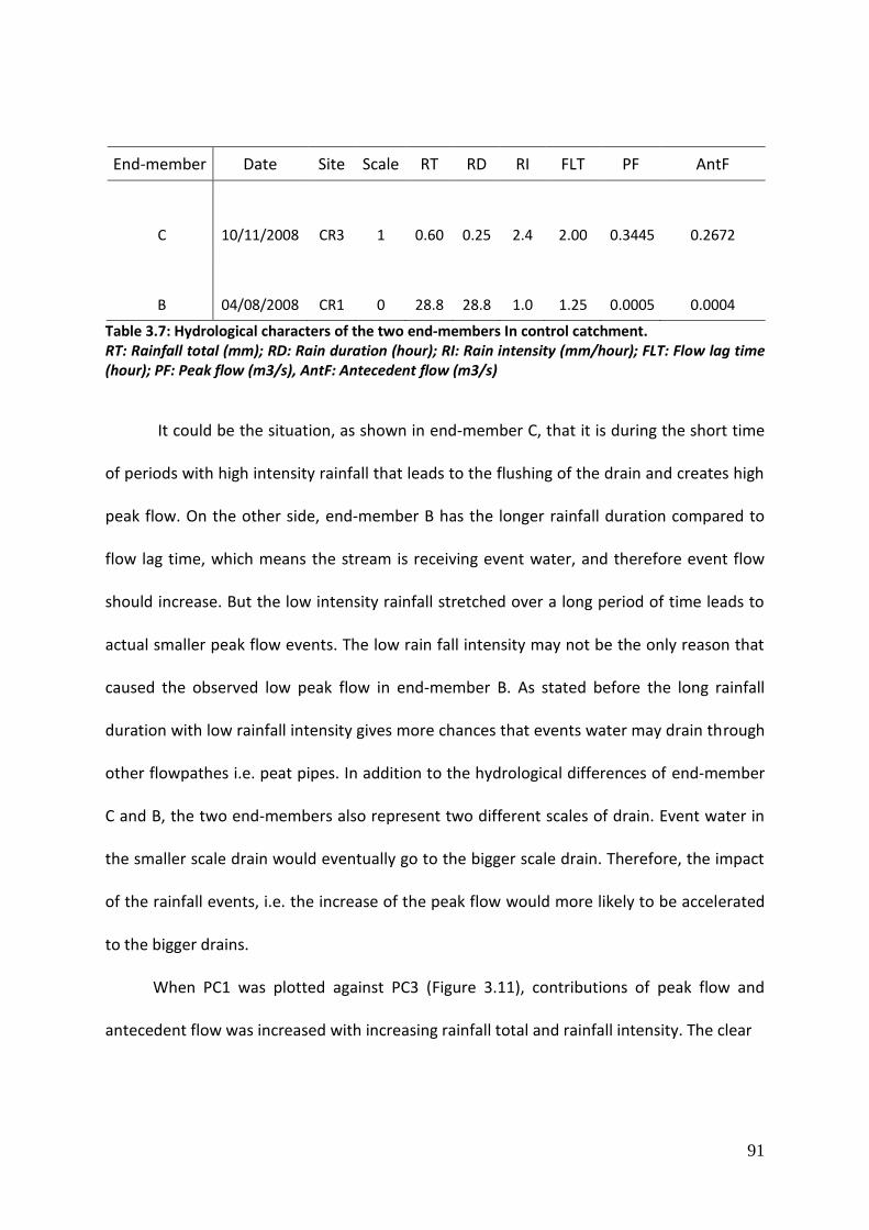
91

End-member Date Site Scale RT RD RI FLT PF AntF

C 10/11/2008 CR3 1 0.60 0.25 2.4 2.00 0.3445 0.2672

B 04/08/2008 CR1 0 28.8 28.8 1.0 1.25 0.0005 0.0004

Table 3.7: Hydrological characters of the two end-members In control catchment. RT: Rainfall total (mm); RD: Rain duration (hour); RI: Rain intensity (mm/hour); FLT: Flow lag time (hour); PF: Peak flow (m3/s), AntF: Antecedent flow (m3/s)

It could be the situation, as shown in end-member C, that it is during the short time

of periods with high intensity rainfall that leads to the flushing of the drain and creates high

peak flow. On the other side, end-member B has the longer rainfall duration compared to

flow lag time, which means the stream is receiving event water, and therefore event flow

should increase. But the low intensity rainfall stretched over a long period of time leads to

actual smaller peak flow events. The low rain fall intensity may not be the only reason that

caused the observed low peak flow in end-member B. As stated before the long rainfall

duration with low rainfall intensity gives more chances that events water may drain through

other flowpathes i.e. peat pipes. In addition to the hydrological differences of end-member

C and B, the two end-members also represent two different scales of drain. Event water in

the smaller scale drain would eventually go to the bigger scale drain. Therefore, the impact

of the rainfall events, i.e. the increase of the peak flow would more likely to be accelerated

to the bigger drains.

When PC1 was plotted against PC3 (Figure 3.11), contributions of peak flow and

antecedent flow was increased with increasing rainfall total and rainfall intensity. The clear

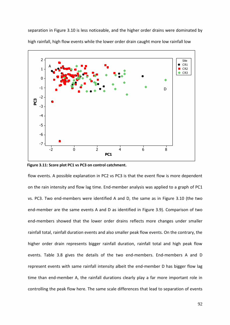
92

separation in Figure 3.10 is less noticeable, and the higher order drains were dominated by

high rainfall, high flow events while the lower order drain caught more low rainfall low

flow events. A possible explanation in PC2 vs PC3 is that the event flow is more dependent

on the rain intensity and flow lag time. End-member analysis was applied to a graph of PC1

vs. PC3. Two end-members were identified A and D, the same as in Figure 3.10 (the two

end-member are the same events A and D as identified in Figure 3.9). Comparison of two

end-members showed that the lower order drains reflects more changes under smaller

rainfall total, rainfall duration events and also smaller peak flow events. On the contrary, the

higher order drain represents bigger rainfall duration, rainfall total and high peak flow

events. Table 3.8 gives the details of the two end-members. End-members A and D

represent events with same rainfall intensity albeit the end-member D has bigger flow lag

time than end-member A, the rainfall durations clearly play a far more important role in

controlling the peak flow here. The same scale differences that lead to separation of events

Figure 3.11: Score plot PC1 vs PC3 on control catchment.

86420-2

2

1

0

-1

-2

-3

-4

-5

-6

-7

PC1

PC

3

CR1

CR2

CR3

Site

A

D

93

in Figure 3.10 were also featured in Figure 3.11. Rainfall character has a greater influence on

first order drains than on zero order drains.

End-member Date Site Scale RT RD RI FLT PF AntF

A 28/03/2008 CR1 0 0.20 0.20 1 1 0.0005 0.0005

D 04/08/2008 CR3 1 28.8 28.8 1 2 0.3247 0.2499

Table 3.8: Hydrological characters of the two end-members In control catchment.RT: Rainfall total (mm); RD: Rain duration (hour); RI: Rain intensity (mm/hour); FLT: Flow lag time (hour); PF: Peak flow (m3/s), AntF: Antecedent flow (m3/s).

The comparison between first three PCs gives an insight into the hydrological changes in

the control catchment during the study period. Of the all the principal components PC4 is

the only principal component that demonstrates a dominant loading for the DOC

concentration changes among all four principal components. The comparisons between PC4

and PC1; and between PC4 and PC2 were therefore plotted to demonstrate patterns of DOC

concentration in the control catchment. PC1 and PC2 are selected because they represent

the two kinds of rainfall event as interpreted earlier: a high rainfall total, high rainfall

duration with high rainfall intensity event; and a high rainfall total, high rainfall duration but

low rainfall intensity event.

94

86420-2

4

3

2

1

0

-1

-2

-3

-4

PC1

PC

4CR1

CR2

CR3

Site

Figure 3.12: Score plot PC1 vs PC4 on control catchment.

5.02.50.0-2.5-5.0

4

3

2

1

0

-1

-2

-3

-4

PC2

PC

4

CR1

CR2

CR3

Site

Figure 3.13: Score plot PC2 vs PC4 on control catchment.

95

In the scatterplots of PC1 vs PC4 and PC2 vs PC4 (Figures 3.12 and 3.13), there are no

clear DOC concentration changes on the PC4 axis that divide between the scales or between

the event types identified.

The scatterplot of PC3 against PC4 (Figure 3.14) is gathered by plots that are patterned

around zero axis. There are no DOC concentration changes that been altered by the PC3

which stand for the increasing flow lag time but decreasing rainfall intensity.

The PCA of the flow event here demonstrated two different kinds of rainfall events that

have different impacts on the peak event flow of the control catchment. However, the

analysis failed to clearly illustrate how the DOC concentration changes between the

catchments.

43210-1-2-3-4

4

3

2

1

0

-1

-2

-3

-4

PC3

PC

4

CR1

CR2

CR3

Site

Figure 3.14: Score plot PC3 vs PC4 on control catchment

96

3.5.2. Comparison of PCs on the experimental catchments

In the experimental catchments four end-members E, F, G, H, were selected. End-

member E has the lowest scores on PC1. End-member F has the highest score on PC2. End-

member G has the lowest score on PC2, while end-member H has the highest score on PC1.

Details of the four end-members are given in Table 5. These four end-member events were

all from the non- blocking periods. Score plots of PC1 against PC2 (Figure 3.15) shows the

trend EF and GH, where events from both the zero order and first order drains plot. Figure

3.15 shows a similar but suppressed pattern compared to Figure 3.9. In Figure 3.15, there

are three parallel lines which divided roughly by each drains that move from E (G) end to F

(H) end. The separation between two different scales of drains observed for the control

catchments (Figure 3.9) still exists, but the boundaries between the drains of different scales

start over lapping on each other in the experimental catchment.

End-member

Date Site Scale RT RD RI FLT PF AntF

E 06/05/200

8 CR6 0 0.2 0.2 1 0.25 0.004 0.004

F 04/08/200

8 CR6 0 28.8 28.8 1 1.25 0.003 0.002

G 03/05/200

8 CR4 1 1 1 1 0.5 0.198 0.075

H 04/08/200

8 CR4 1 28.8 28.8 1 2 0.046 0.043

Table 3.9: Hydrological characters of the four end-members in experimental catchment

RT: Rainfall total (mm); RD: Rain duration (hour); RI: Rain intensity (mm/hour); FLT: Flow lag time (hour); PF: Peak flow (m3/s), AntF: Antecedent flow (m3/s)

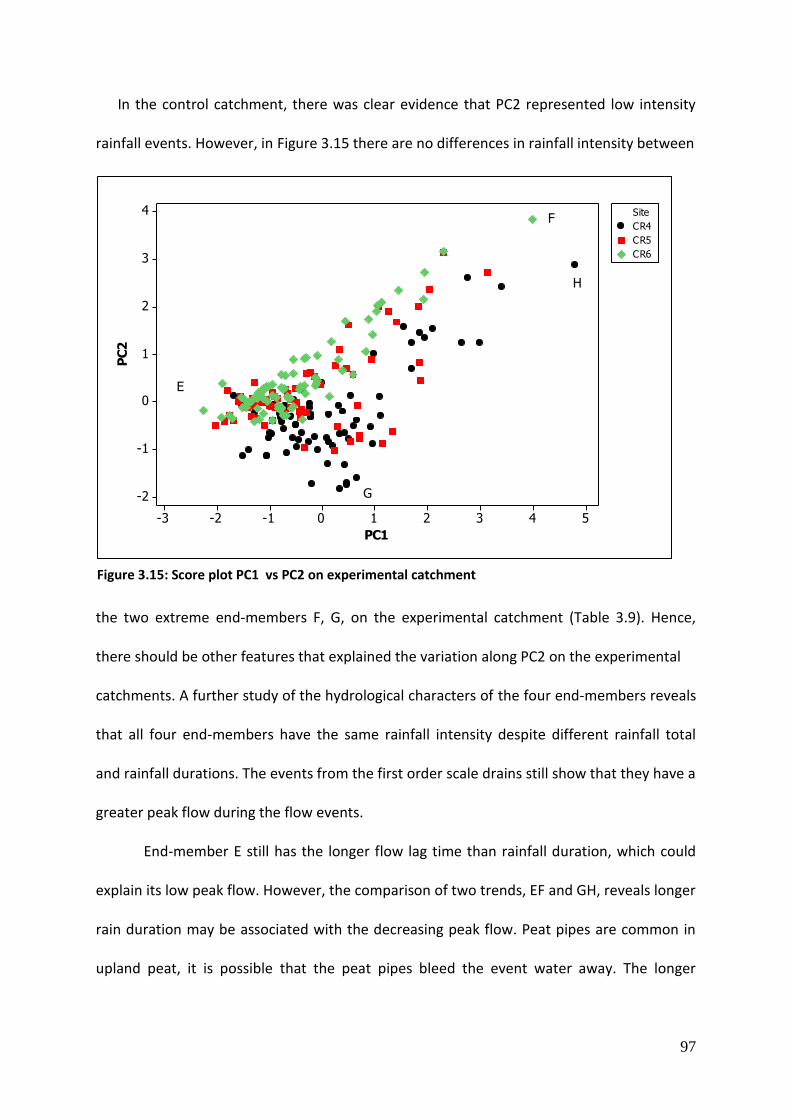
97

In the control catchment, there was clear evidence that PC2 represented low intensity

rainfall events. However, in Figure 3.15 there are no differences in rainfall intensity between

the two extreme end-members F, G, on the experimental catchment (Table 3.9). Hence,

there should be other features that explained the variation along PC2 on the experimental

catchments. A further study of the hydrological characters of the four end-members reveals

that all four end-members have the same rainfall intensity despite different rainfall total

and rainfall durations. The events from the first order scale drains still show that they have a

greater peak flow during the flow events.

End-member E still has the longer flow lag time than rainfall duration, which could

explain its low peak flow. However, the comparison of two trends, EF and GH, reveals longer

rain duration may be associated with the decreasing peak flow. Peat pipes are common in

upland peat, it is possible that the peat pipes bleed the event water away. The longer

Figure 3.15: Score plot PC1 vs PC2 on experimental catchment

543210-1-2-3

4

3

2

1

0

-1

-2

PC1

PC

2

CR4

CR5

CR6

Site

E

F

G

H

98

rainfall event, the more likely peat pipes would have more impact on the flow. Also, the

bigger scale the drain is, the bigger impact of these peat pipes would be.

Scatterplots of PC1 vs PC2 were plotted with blocking status and site on experimental

catchment (Figure 3.16). There is very clear separation between zero order drains on the

plots, i.e. the yellow and purple groups that represent events from drain CR6 before and

after blocking. Two separate trend lines can also be seen for the CR5. These separate trend

lines show the impact of the blocking on zero order drains. After blocking, the zero order

drains were shifted towards higher peak flows.

However, this separation due to blocking can’t be seen for the first order drain (Figure 3.16).

Instead, overlapped plots for the first order drain and lack of separation of events before

and after blocking indicate that drain blocking didn’t necessarily change the event flow

character on the first order drain. A lack of change in event flow character for the first order

Figure 3.16: Score plot PC1 vs PC2 on experimental catchment.

543210-1-2-3

4

3

2

1

0

-1

-2

PC1

PC

2

CR4 n

CR4 y

CR5 n

CR5 y

CR6 n

CR6 y

Site Blocked?

99

drain may indicate that there are more chances the peat pipes are operating at this scale.

The existence of peat pipes would lead to the event water going through the subsoil

pathways and so be unaffected by blocking.

The separation of the different scales observed on PC2 can also been observed by the

score plot of PC3 vs PC2 and score plot of PC4 vs PC2 (Figure 3.17 and Figure 3.18).

However, the same separation cannot be observed for either PC3 vs PC1 or PC4 vs PC1.

Following the earlier analysis of principal components (Table 3.5), PC3 represents for

increasing flow lag time and decreasing rain intensity, and PC4 represents the DOC

concentration changes.

On Figure 3.17, the majority of the events plot on the positive end of PC3 while a separation

between first and zero order was made on PC2. Among all the events that were selected in

this analysis, the contributions of the flow lag time to the events concentration changes

Figure 3.17: Score plot PC3 vs PC2 on experimental catchment.

43210-1-2-3-4-5

2

1

0

-1

-2

-3

-4

-5

-6

-7

PC2

PC

3

0

1

Scale

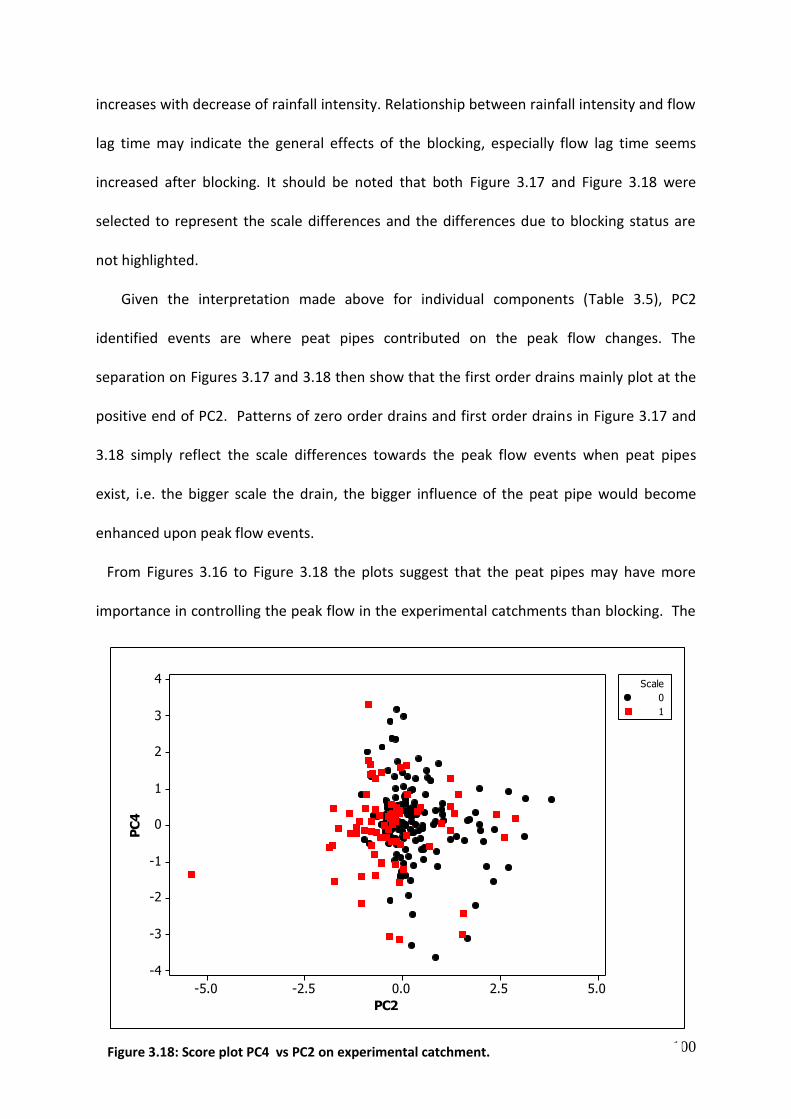
100

increases with decrease of rainfall intensity. Relationship between rainfall intensity and flow

lag time may indicate the general effects of the blocking, especially flow lag time seems

increased after blocking. It should be noted that both Figure 3.17 and Figure 3.18 were

selected to represent the scale differences and the differences due to blocking status are

not highlighted.

Given the interpretation made above for individual components (Table 3.5), PC2

identified events are where peat pipes contributed on the peak flow changes. The

separation on Figures 3.17 and 3.18 then show that the first order drains mainly plot at the

positive end of PC2. Patterns of zero order drains and first order drains in Figure 3.17 and

3.18 simply reflect the scale differences towards the peak flow events when peat pipes

exist, i.e. the bigger scale the drain, the bigger influence of the peat pipe would become

enhanced upon peak flow events.

From Figures 3.16 to Figure 3.18 the plots suggest that the peat pipes may have more

importance in controlling the peak flow in the experimental catchments than blocking. The

Figure 3.18: Score plot PC4 vs PC2 on experimental catchment.

5.02.50.0-2.5-5.0

4

3

2

1

0

-1

-2

-3

-4

PC2

PC

4

0

1

Scale

101

different scale drains, the higher order drains were more likely to see the accumulated peak

flow but at the same time are also more affected by potential existence of peat pipes.

Therefore, drain blocking is more likely to fail to control the peak flow on the higher order

drains in the control catchment.

In the experimental catchment, the blocking effects can be observed on the changes

of flow lag time. Figures 3.19 and 3.20 show the comparison of the blocked and unblocked

drains in terms of hydrological changes and flow lag time with rainfall intensity. PC1

represents the events when the peak flow increased with increasing rainfall while PC2

represents the events where peak flow decreased with increasing rainfall. In both situations,

flow lag time increased with decreasing rainfall intensity after blocking while the unblocked

periods have data plotting across the range of PC3.

Figure 3.19: Score plot PC3 vs PC2 on experimental catchment.

5.02.50.0-2.5-5.0

2

1

0

-1

-2

-3

-4

-5

-6

-7

PC2

PC

3

n

y

Blocked?

102

The separation of blocked and unblocked event periods was less apparent when PC1

and PC2 were plotted against PC4. The small apparent separation on PC4 indicates blocking

is less effective at altering the DOC concentration change across an event (Figures 3.21 and

3.22). Blocking is largely affected by the potential peat pipes which means it failed to

maintain control on the peak flow in the higher order drain of the experimental catchment.

Therefore, the variations of DOC concentration changes are less clear in Figures 3.21 and

3.22.

Figure 3.20: Score plot PC3 vs PC1 on experimental catchment.

543210-1-2-3

2

1

0

-1

-2

-3

-4

-5

-6

-7

PC1

PC

3

n

y

Blocked?

103

Figure 3.21: Score plot PC4 vs PC1 on experimental catchment.

Figure 3.22: Score plot PC4 vs PC2 on experimental catchment.

543210-1-2-3

4

3

2

1

0

-1

-2

-3

-4

PC1

PC

4n

y

Blocked?

5.02.50.0-2.5-5.0

4

3

2

1

0

-1

-2

-3

-4

PC2

PC

4

n

y

Blocked?

104

3.5.3 PCA including other chemical parameters

To assess the potential flow path change that brings about the observed event flow

and DOC concentration changes, a single PCA was performed including: pH, conductivity,

DOC concentration, and applying the same rules described above (section 3.3). Upon

analysis two principal components were selected. Together the two selected PCs explained

80.4% of the variance in the data (Table 3.9). The first component (PC1) is a contrast

between pH and DOC concentration changes. The second principal component (PC2) has

high negative loading for the conductivity. For PC2, the loadings DOC concentration change

and pH are relatively small compared to that for conductivity; therefore, PC2 is dominated

by the conductivity loadings.

Variable PC1 PC2

DOC concentration 0.647 0.325

pH -0.665 -0.202

Conductivity 0.373 -0.924

Eigenvalue 1.489 0.924

Proportion 0.497 0.308

Cumulative 0.497 0.804

Table 3.10: The first two principal components of Cronkley Fell.

Comparing PC1 and PC2 (Figures 3.23 and 3.24) confirms the interpretation of the

components given above. The majority of the variation is parallel to PC1, i.e. variation only

in DOC concentration changes. Separation gradually happens when moving towards the

higher end of PC1, which indicated the inverse relation between two scales of the

105

catchment and DOC concentration changes (Figure 3.23). Increases in pH occurred with

increased scale. After blocking, the majority of the data plots at the negative end of PC2

which indicates an increase in event water conductivity after blocking (Figure 3.24).

Whisker-plots of pH and conductivity for both scale before and after blocking shows

that in the zero order drains, both pH and conductivity increased after blocking. In the first

order drains, pH of event water decreased while the conductivity increased after blocking

(Figure 3.25 and Figure 3.26).

Figure 3.23: Score plots of PC1 VS PC2 on different drain scales.

3210-1-2-3-4

3

2

1

0

-1

-2

-3

-4

-5

PC1

PC

2

0

0

0

1

Scale

106

Figure 3.24: Score plots of PC1 VS PC2 on blocking statue.

Figure 3.25: Whisker box of pH on two different scale drains before and after blocking.

3210-1-2-3-4

3

2

1

0

-1

-2

-3

-4

-5

PC1

PC

20

0

n

y

Blocked?

Scale

Blocked?

10

ynyn

8

7

6

5

4

3

pH

107

An ANOVA was applied on both PC1 and PC2 to investigate impacts of the

experimental factors (Table 3.11). The majority of the variances of PC1 were explained by

scale (38.7%). While PC2 mostly varies with blocking. This indicates the DOC concentration

changes may be mainly controlled by the scale difference, while the blocking effects

changed the conductivity. Worrall et al. (2002) found higher conductivity water was

associated with ‘old water’, whereas the low conductivity at high flow represented the rain

water. The shift from the new to old water after blocking among this events analysis may

imply that the DOC composition changes, blocking brings event water that includes a

greater component of deeper soil water.

Figure 3.26: Whisker box of conductivity on two different scale drains before and after blocking

Scale

Blocked?

10

ynyn

90

80

70

60

50

40

30

20

10

0

Co

nd

ucti

vit

y

108

PC1 PC2

source DF P Portion source DF P Portion Month 1 <0.001 3.00% Month

<0.001 1.61%

Scale 1 <0.001 38.74% Scale

<0.001 5.15% Blocked? 1 0.001 0.04% Blocked?

<0.001 11.45%

Scale* Blocked? 1 <0.001 3.74% Year

<0.001 2.02%

Error 751

Error Total 755

Total

R-Sq =45.73% R-Sq =20.79%

Table 3.11: ANOVA of first two components.

3.6. Results of DOC flux

Variations of DOC flux changes over selected events can be observed on the whisker plot

(Figure 3.27) before and after blocking. DOC flux changes over events decreased by 55.6%

after blocking on both control and experimental catchments. During the peak flow events,

rapid rain flow brought more rain water going through the system and, the DOC

concentration decreased after blocking (Figure 3.4). As mentioned before, the events water

went into the deep soil path ways in the higher order drains in the experimental catchment,

which leads to the decrease in the peak flow. At the same time, the DOC concentrations

changes were varied on a much bigger scale i.e. 400% variations during events. Therefore,

although there are situations that both DOC concentration changes and event flow are

decreasing, DOC flux changes can still been observed an average suppression of 55.6%.

109

Similar to the DOC concentration changes in the control catchment, the DOC flux

changes also show differences between different scales in the control catchment (Figure

3.28). Only this time, the flux changes seem much bigger in zero order drains than the first

order drain. The differences in flux changes could simply be following the same depression

of DOC concentration changes observed in the control catchments (Figure 3.4). The decline

of flux changes from zero order drain to first order drain could be caused by two potential

event flow changes: either the event flow would be increased from zero order drain to first

order drain, or the decline of the event flow should be much smaller compared to the

decline of concentration changes from zero order to first order drain. The smaller changes

in event flow in the control catchment in turn indicate that the DOC concentration changes

Figure 3.27: DOC flux changes before and after blocking.

yn

5.0

2.5

0.0

-2.5

-5.0

-7.5

Blocked?

DO

C F

lux c

ha

ng

e (

gC

)

110

are caused by scale difference between two different scale drains. A further PCA was then

performed on the data set.

The comparison of the DOC flux changes before and after blocking in experimental

catchment in between two scales is showed in Figure 3.29. In Figure 3.29, CR4, a first-order

drain, the DOC flux change over events is smaller after blocking. Although CR5 and CR6 are

zero order drains, only CR6 shows the same change as the first order drain. Instead of

showing smaller changes as its paired drain, CR5 showed bigger, positive flux changes after

blocking. By comparing to the DOC concentration changes in Figure 3.7, it is clear that DOC

concentration changes were getting smaller in all three drains in experimental catchment.

The increased DOC flux in CR5 indicated more of a difference that caused by the drain itself,

as mentioned above, i.e. the presence of peat pipes. The existence of peat pipes would

cause event water to run through sub soils. These flow path changes would minimize the

Figure 3.28: DOC flux changes in control catchment. The upper whiskers (top 25% of data) of CR 1 is too close to up boundary of interquartile box to shown in figure, which duo to the lower data point compare to other two drains.

CR3CR2CR1

100

50

0

-50

Site

DO

C F

lux c

ha

ng

e (

gC

)

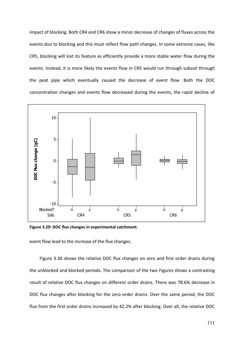
111

impact of blocking. Both CR4 and CR6 show a minor decrease of changes of fluxes across the

events duo to blocking and this must reflect flow path changes. In some extreme cases, like

CR5, blocking will lost its feature as efficiently provide a more stable water flow during the

events. Instead, it is more likely the events flow in CR5 would run through subsoil through

the peat pipe which eventually caused the decrease of event flow. Both the DOC

concentration changes and events flow decreased during the events, the rapid decline of

event flow lead to the increase of the flux changes.

Figure 3.30 shows the relative DOC flux changes on zero and first order drains during

the unblocked and blocked periods. The comparison of the two Figures shows a contrasting

result of relative DOC flux changes on different order drains. There was 78.6% decrease in

DOC flux changes after blocking for the zero-order drains. Over the same period, the DOC

flux from the first order drains increased by 42.2% after blocking. Over all, the relative DOC

Figure 3.29: DOC flux changes in experimental catchment.

Site

Blocked?

CR6CR5CR4

ynynyn

10

5

0

-5

-10

DO

C F

lux c

ha

ng

e (

gC

)

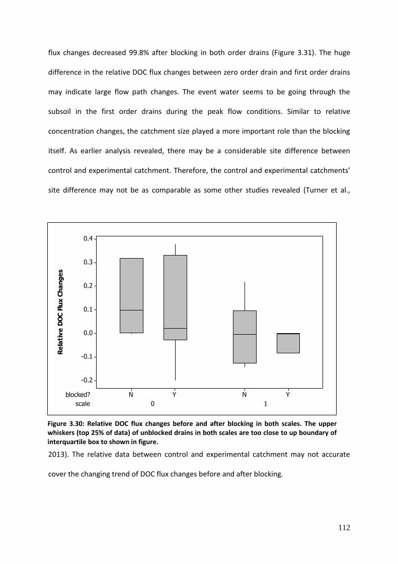
112

flux changes decreased 99.8% after blocking in both order drains (Figure 3.31). The huge

difference in the relative DOC flux changes between zero order drain and first order drains

may indicate large flow path changes. The event water seems to be going through the

subsoil in the first order drains during the peak flow conditions. Similar to relative

concentration changes, the catchment size played a more important role than the blocking

itself. As earlier analysis revealed, there may be a considerable site difference between

control and experimental catchment. Therefore, the control and experimental catchments’

site difference may not be as comparable as some other studies revealed (Turner et al.,

2013). The relative data between control and experimental catchment may not accurate

cover the changing trend of DOC flux changes before and after blocking.

Figure 3.30: Relative DOC flux changes before and after blocking in both scales. The upper whiskers (top 25% of data) of unblocked drains in both scales are too close to up boundary of interquartile box to shown in figure.

scale

blocked?

10

YNYN

0.4

0.3

0.2

0.1

0.0

-0.1

-0.2

Re

lati

ve

DO

C F

lux C

ha

ng

es

113

3.7. PCA of the hydrological changes during events

The first four principal components had eigenvalues greater than one, and the first

principal component with an eigenvalue less than one was also selected. The first four

components together explained 76.8% of the original variance in the dataset, while PC1 and

PC2 explained about half of the original variance. All the data was z transferred and

therefore PC1 represents a major interaction between rainfall total, rainfall duration and

peak flow, antecedent flow rather than variable normalization. PC2 is controlled by positive

loadings of peak flow, antecedent flow and negative loadings of rainfall total and rainfall

intensity. PC3 is determined by a pair of strong positive loadings: flow lag time, DOC flux

changes. PC4 is represented by high positive loadings of rain intensity and DOC flux changes.

A similar hydrological behavior was performed here to the early analysis of the DOC

concentration changes (Table 3.5). According to the dominant loadings of four components,

Figure 3.31: Relative DOC flux changes before and after blocking.

YN

0.5

0.4

0.3

0.2

0.1

0.0

-0.1

-0.2

-0.3

blocked?

Re

lati

ve

DO

C F

lux C

ha

ng

es

114

PC1 represent the positive effects of direct rain fall to the event flow. PC2 demonstrates a

negative relation between rainfall and events flow, events flow is more controlled by its

antecedent flow and additional contribution from other sources rather than rainfall. As for

the PCA of DOC concentration changes, the PC1 and PC2 group together and represent the

hydrological changes while the PC3 and PC4 group together and represent the DOC flux

changes.

Variable PC1 PC2 PC3 PC4

Z Rain Total (mm)_ 0.521 -0.434 -0.1 0.009

Z Rain Duration (hours)_ 0.527 -0.416 0.008 -0.161

Z Rain Intensity (mm/hour)_ -0.058 -0.059 -0.487 0.756

Z Flow lag time 0.222 0.145 0.599 0.112

Z Peak flow 0.389 0.535 -0.043 0.129

Z Antecedent flow 0.405 0.547 -0.1 -0.002

Z Time between events -0.288 0.058 0.231 -0.139

Z DOC flux changes 0.017 -0.159 0.573 0.595

Eigenvalue 2.1077 1.7682 1.2939 0.972

Proportion 0.263 0.221 0.162 0.121

Cumulative 0.263 0.484 0.646 0.768

Table 3.12: Hydrological loadings of first four PCs.

Where absolute loading values bigger than 0.400 were considered as dominate loadings and marked red. In Table 3.12, PC3 represents the positive relationship between flow lag time and

DOC flux changes, the DOC flux change increase with increasing flow lag time which may

indicate the effects of the blocking. Loadings of PC4 highlight the interaction between rain

intensity and DOC flux changes, the intense rainfall contributes to the positive DOC flux

changes.

In the first group PC1 vs PC2, the divisions between the rainfall and events flow on

115

PC2 suggest that PC2 may indicate other sources or caused the increase of the event flow.

Similar relationship between loadings of event flow and rainfall is also observed in the PCA

of DOC concentration changes (Table 3.6). Brown et al. (1999) stated the contribution of

rapid shallow flow to the events water is more likely to cause the DOC changes of events

water than the changes in rainfall causing changes in the DOC flux change. This is especially

so when the events water was mostly alter by the high intensity rainfall with the influence

of the rainfall is often inversely related to the catchment size. The observations of PC1 and

PC2 in both DOC concentration changes and DOC flux changes were most likely reflected by

the same mechanism as Brown et al. (1999) proposed. PC1 represents the contribution of

high intensity rainfall to the event flow and therefore contributed to the DOC flux changes.

Loading from PC2 therefore represented the rapid shallow flow changes which contributed

mostly to the event flow.

When blocking is applied to the sites, the results for DOC concentration changes

suggested a positive effect due to events flow. In term of DOC flux changes in this section, it

is expected a similar impact of the blocking may also reflects on the loadings. To test this

hypothesis, an ANOVA was performed on the all four PCs with the changes of hydrological

variances. Comparisons of ANOVA results in the first two components are listed in Table

3.13. In PC1, only peak flow, antecedent flow, rainfall intensity and flow lag time were

found to be significant factors which in total explained 76.74% variances of PC1. Among

these four significant factors, rainfall intensity explained majority of the variances (74.35%),

while flow lag time explained the smallest of variances only 3.25%. In PC2, rainfall total,

peak flow, antecedent flow, scale, blocked, rainfall intensity, flow lag time together

explained 98.98% of the variance. Among the significant factors in PC 2, rainfall total

explained more than half of the total variance (51.90%). Scale explained only 0.13% of the

116

variance of PC2 which is the least important factor in the PC2. Comparison between PC1

and PC2 indicates blocking effects is limited on PC1 while it is significant on PC2. It is clear

ANOVA of PC1 reflected contribution of the high intensity rain fall to the events flow as both

the rainfall intensity and peak flow are among the significant variances.

The difference between PC1 and PC2 is mainly on the variance of scale and blocking.

Scale is not a significant factor of the variances of PC1 while it is a significant factor in PC2.

Variances between PC1 and PC2 reflected the hypothesis of the identification of each

component earlier, which PC1 reflects the events high intensity rainfall dominated the event

flow and PC2 reflects the event of rapid shallow flow, which dominated the event flow.

Differences of two kinds of flow events are reflected by the blocking effects. In the events of

high rainfall intensity dominated events, the blocking is not a significant factor contributing

to events, nor is the scale factor. As an observation of Brown et al., (1999), scale should be

an important factor during the high intensity rainfall. A one way ANOVA of PC1 with scale as

a factor found scale is still a significant factor contributing to PC1 which explained

approximately 10% of variances of PC1. It is only when the blocking has been introduced to

Component PC1 PC2

Source DF P Portion DF P Portion Rain Total NS NS NS 1 <0.001 5.19% Peak flow 1 <0.001 4.19% 1 <0.001 15.43% Antecedent flow 1 <0.001 7.27% 1 <0.001 21.67% Scale NS NS NS 1 <0.001 0.13% Blocked? NS NS NS 1 <0.001 0. 76% Z Rain Intensity 66 <0.001 74.35% 66 <0.001 7.93% Z Flow lag time 10 <0.001 3.25% 10 1.34% Error 331

10.94% 328

0.85%

Total 409

409

R-Sq = 81.18% R-Sq = 99.16%

Table 3.13: ANOVA of first two principal components, NS: not significant variances.

117

the ANOVA that scale, blocking or interaction between these two were found not be

significant. As the blocking is a significant factor contributing to the variance of PC2, it is

therefore highlighted that positive blocking effects during the event flow are limited to the

rapid shallow flow contribution. While similar effects (blocking) may be applied to high

intensity rainfall events such as PC1, blocking effects may only eliminate the scale effects

that may have brought on the event flow, but overall were not as an efficient control of the

event flow itself. That means in PC1 blocking may have brought up the water table depth in

both scales of drains which eliminated the potential scale effect on the events flow during

the high intensity rainfall, but blocking would have failed to control the event flow as both

scales of drains would quickly have overflown the potential buffer supplied by the drain

blocking.

In PC3, antecedent flow, blocking, rainfall intensity, and flow lag time together

explained 79.05% of the variances. Rainfall intensity in PC3 explained half of the total

variance, while blocking explained the least of variances (6.89%). In PC4, peak flow,

antecedent flow, scale, blocking, rainfall intensity and flow lag time together explained

93.50% of total variances. Rainfall intensity in the PC4 explained 83.11% of the variance.

Scale is the least important factor among all the significant variances as it only explained

0.98% of the variances.

Component PC3 PC4

Source DF P Portion DF P Portion Z Peak flow NS 1 <0.001 0.0226 Z Antecedent flow 1 <0.001 0.0976 1 <0.001 0.0266 Scale NS 1 <0.001 0.0098 Blocked? 1 <0.001 0.0689 1 <0.001 0.0526 Z Rain Intensity 66 <0.001 0.5251 66 <0.001 0.8311 Z Flow lag time 10 <0.001 0.2119

<0.001 NS

Error 331

0.2308 339

0.0574 Total 409

409

R-Sq = 83.05% R-Sq = 97.20%

Table 3.14: ANOVA of principal component 3 and 4, NS: not significant variances.

118

PC3 and PC4 indicated that rainfall intensity is the key factor that controls the DOC flux

changes (Table 3.14). Blocking is expected to be an efficient land management appears to

control the event flux. As shown in the Table 3.13, the blocking effects are significant but

the majority of the flux changes are still controlled by the rainfall intensity. In other words,

the blocking may not be as efficient as expected for controlling the DOC flux changes when

compared to the characteristics of the event itself. The above section of DOC concentration

changes (section 3.2) took the hypothesis that an additional flow path may be involved in

the land management, which leads the event flow drain through the additional flow path

(i.e. peat pipes). This hypothesis maybe also applied to analysis of the DOC flux changes

here, the effects of the blocking is limited by the potential flow paths.

3.7.1. Comparison of PCs in control catchment

The score plots of PC1 against PC2 identified four end-members – a, b, c, and d

(Figure 3.32). The direction of ab generally represents the zero order drains (CR1, CR2),

while the cd trend is gathered by the zero order drains (CR3). The comparison of zero order

drains and first order drains found loading plots of first order drains exist both in area ab

and area cd. On Figure 30, end-member a has the lowest score on PC1. As mentioned

earlier, PC1 is dominated by strong positive loadings of total rainfall, rainfall duration, peak

flow and antecedent flow. End-member b has the lowest score on PC2, which is marked by

high event flow, low rainfall events. End-member c has highest score on the PC2 and end-

member d has the highest score on PC1. The details of the four individual end-members are

119

given in Table 3.15. It is found in Table 3.14, that all four end-members a, b, c, d are exactly

same as the earlier analysis in DOC concentration changes in Table 3.6. The trend line of

zero order drain (Line ab) and the trend line of first order drain (Line cd) were exactly the

same as the study of the control catchment in the analysis of DOC concentration changes

(Figure 3.9). The patterns of two Figures are rotated 90 degrees by the differences of two PC

2s, the earlier one has the positive loadings of rainfall total and rainfall duration and

negative loadings of peak flow, antecedent flow (Table 3.5), but the current one has the

positive loadings of peak flow and antecedent flow and negative loadings of rainfall total

and rainfall duration (Table 3.11). The result of the earlier analysis can therefore imply the

following here: during the hydrological peak flow events the event flow is determined by

the different rainfall intensities and differences of the flow lag time. The flow lag time is

determined by the different scale of the drains. The study also indicates that the potential

flow path would also influence on the event flow typically on the higher order drains. In the

Figure 3.32, the almost paralleled lines among higher order drain that moves between line

ab and cd indicates this potential of the other flow paths causing the event flow to

decrease.

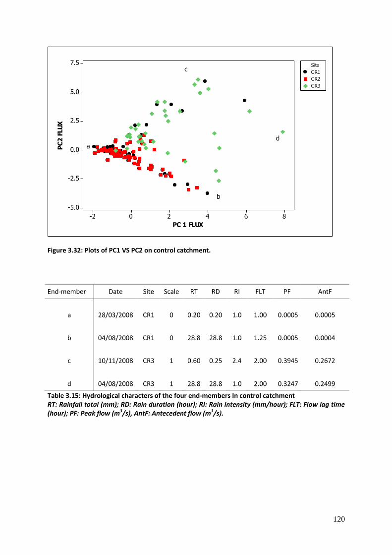
120

86420-2

7.5

5.0

2.5

0.0

-2.5

-5.0

PC 1 FLUX

PC

2 F

LU

X

CR1

CR2

CR3

Site

a

b

c

d

Figure 3.32: Plots of PC1 VS PC2 on control catchment.

Table 3.15: Hydrological characters of the four end-members In control catchment RT: Rainfall total (mm); RD: Rain duration (hour); RI: Rain intensity (mm/hour); FLT: Flow lag time (hour); PF: Peak flow (m3/s), AntF: Antecedent flow (m3/s).

End-member Date Site Scale RT RD RI FLT PF AntF

a 28/03/2008 CR1 0 0.20 0.20 1.0 1.00 0.0005 0.0005

b 04/08/2008 CR1 0 28.8 28.8 1.0 1.25 0.0005 0.0004

c 10/11/2008 CR3 1 0.60 0.25 2.4 2.00 0.3945 0.2672

d 04/08/2008 CR3 1 28.8 28.8 1.0 2.00 0.3247 0.2499

121

Comparison of PC3 VS PC4 would show the DOC flux changes in the control

catchment during the events, as both of two components including the high loadings of DOC

flux changes. Despite six individual events in the first order drains, the majority of data

plots in both order drains are moving towards the positive ends of both axes. As both PC3

and PC4 have the positive loading of DOC flux changes, DOC flux changes were increasing

with increasing rainfall intensity and flow lag time in control catchment.

Figure 3.33: PC3 vs PC4 in control catchment.

7.55.02.50.0-2.5-5.0

6

5

4

3

2

1

0

-1

-2

PC3 FLUX

PC

4 F

LU

X

CR1

CR2

CR3

Site

122

3.7.2. Comparison of PCs in experimental catchment

Similar to the analysis of the data from the control catchments, the analysis of the

data from the experimental catchment is based on the two separate groupings of principal

components - PC1 vs PC2 dominated by hydrological characteristics and PC3 vs PC4

dominated by changes in DOC. In the plots of PC1 against PC2 (Figure 3.34), four end-

members e, f, g, h were identified. As seen earlier, the four end-members are exactly as in

Figure 3.15, therefore the values of individual end-member can be found in Table 3.9.

Similar patterns between control (Figure 3.32) and experimental catchment (Figure 3.34)

were observed before and after blocking. There are clear separations between blocked and

unblocked periods in the zero order drains (CR5, CR6). Event flow changes before and after

blocking in first order drain (CR4). As mentioned before, the unclear transition in first order

drain implies there may be more influence of additional flow path on the first order drains,

Figure 3.34: Plots of PC 1 vs PC2 before and after blocking in individual sites in experimental catchment.

543210-1-2-3

2

1

0

-1

-2

-3

-4

PC 1 FLUX

PC

2 F

LU

X

CR4 n

CR4 y

CR5 n

CR5 y

CR6 n

CR6 y

Site Blocked?

e

f

g

h

123

which limited the blocking effects to maintain the stable water table.

Loading plots of PC3 against PC4 in experimental catchments (Figure 3.35) shows

dramatic changes on patterns to that observed for the control catchment (Figure 3.33). With

both order drains plotting at the end of the negative end of the PC4. The plots showing that

both order drains were under the positive influence of rainfall intensity and flow lag time in

the control catchment (Figure 3.33) are not obvious in the experimental catchment (Figure

3.35). Figure 3.35 shows the majority of the events were plotted at the negative end of PC4

and parallel to the axis of PC3. There are no clear separations between unblocked and

blocked events at each site. Figure 3.35 suggested that the influence of the rainfall intensity

on DOC flux changes were not present, i.e. there are no clear trends on PC4 axis. As shown

on Figure 3.17, blocking have the positive effects on maintained peak flow changes in

experimental catchment despite high rainfall intensity. In Figure 3.35, the DOC flux changes

is also shown been less infected by rainfall intensity. In section 3.5.2, it has been shown that

flow lag time increased after blocking. This is also shown in Figure 3.35 as the majority of

data were parallel to PC3. However, there is no direct trend of DOC flux changes after

blocking events through the blocking has shown a significant impact on changes in flow lag

time. The potential flow path ways have appeared to limit the effects of blocking on DOC

flux changes.

124

3.7.3. Comparison of the pH and conductivity

To estimate the potential flow path changes, PCA were performed that included DOC

flux, pH and conductivity. Two components were selected and together they explained

72.5% of the data set (Table 3.16). PC1 represented the negative correlation between DOC

flux change and pH. Loadings in PC1 are dominated by positive loading of pH and negative

loading for conductivity. PC2 is made of the positive loading of pH and negative DOC flux

changes. Therefore, PC1 stands for the event waters that have high pH and low conductivity

Variable PC1 PC2

pH 0.639 0.418

Conductivity -0.701 -0.028

DOC Flux 0.317 -0.908

Eigenvalue 1.1805 0.9941

Proportion 0.394 0.331

Cumulative 0.394 0.702

Table 3.16: First two components in terms of DOC flux.

Figure 3.35: Plots of PC3 vs PC4 in experimental catchment before and after blocking in individual site.

210-1-2-3-4-5

7

6

5

4

3

2

1

0

-1

-2

PC3 FLUX

PC

4 F

LU

X

CR4 n

CR4 y

CR5 n

CR5 y

CR6 n

CR6 y

Site Blocked?

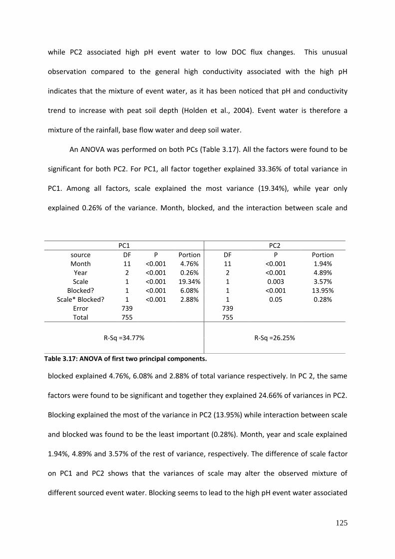
125

while PC2 associated high pH event water to low DOC flux changes. This unusual

observation compared to the general high conductivity associated with the high pH

indicates that the mixture of event water, as it has been noticed that pH and conductivity

trend to increase with peat soil depth (Holden et al., 2004). Event water is therefore a

mixture of the rainfall, base flow water and deep soil water.

An ANOVA was performed on both PCs (Table 3.17). All the factors were found to be

significant for both PC2. For PC1, all factor together explained 33.36% of total variance in

PC1. Among all factors, scale explained the most variance (19.34%), while year only

explained 0.26% of the variance. Month, blocked, and the interaction between scale and

blocked explained 4.76%, 6.08% and 2.88% of total variance respectively. In PC 2, the same

factors were found to be significant and together they explained 24.66% of variances in PC2.

Blocking explained the most of the variance in PC2 (13.95%) while interaction between scale

and blocked was found to be the least important (0.28%). Month, year and scale explained

1.94%, 4.89% and 3.57% of the rest of variance, respectively. The difference of scale factor

on PC1 and PC2 shows that the variances of scale may alter the observed mixture of

different sourced event water. Blocking seems to lead to the high pH event water associated

PC1 PC2

source DF P Portion DF P Portion Month 11 <0.001 4.76% 11 <0.001 1.94%

Year 2 <0.001 0.26% 2 <0.001 4.89% Scale 1 <0.001 19.34% 1 0.003 3.57%

Blocked? 1 <0.001 6.08% 1 <0.001 13.95% Scale* Blocked? 1 <0.001 2.88% 1 0.05 0.28%

Error 739

739 Total 755

755

R-Sq =34.77% R-Sq =26.25%

Table 3.17: ANOVA of first two principal components.

126

with low DOC flux changes. This shows that the blocking alters the flow paths which leads to

the event water going through the deep soil which initially decreased the variation in the

DOC flux changes.

3.8 Conclusions

Blocking was found to be a significant factor impacting both DOC concentration and

DOC flux changes over runoff events. However, the effects of blocking during the peak flow

events were more controlled by the flow path and scale within any catchment. Unlike the

reverse relationship between the DOC concentration and scale shown by the Brown et al.

(1999), this events analysis found the DOC concentration change over events increased

with scale after blocking.

The results showed that the blocking was a significant influence on the DOC flux and

DOC concentration changes over events by controlling the event flow. These event analyses

found rainfall total and peak flow have the biggest impact on changing peak flow of the

events. However, rainfall intensity and relationship between flow lag time and rainfall

duration also alter peak flow throughout the events. When the rainfall duration is smaller

than the flow lag time, the higher rainfall intensity the higher peak flow would be. When

events have the same rainfall intensity, the higher order drain would have the higher peak

flow. When rainfall duration is longer than flow lag time, the peak flow increased with scale.

The blocking method used here was based on peat dams, which, during the storm

events, water would most likely overtop the dam and continuing running through the drain.

Alternatives was to build a series of dams with the aim to encourage revegetation, therefore

events water during significant flow events would overflow the drain cross the vegetation of

127

the peat (Armstrong et al., 2012). Further studies would therefore concentrate on the

vegetation restorations which may impacts on the DOC releasing.

128

Chapter 4 Revegetation

4.1 Introduction

The earlier chapters have discussed the role of peatland as a carbon sink and point out

that peatland is a sensitive system that requires specific climate conditions and poor

drainage to grow, develop and remain stable. Drainage in upland peat therefore would lead

to a negative impact on the ecosystem and could lead to a transition from a carbon sink to a

carbon source. Moreover, studies show that not only the drainage but also burning and

grazing would not only lead to increases in surface runoff but also increased soil erosion,

which would enhance the net dissolved organic carbon (DOC) export (Bellamy et al. 2012;

Brown et al. 2015). Cutover surface plants (Evans and Brazier, 2005) or cool burning (Clay et

al., 2009) have been shown to lead to either the absence of the vegetation or changes to

the colonised vegetation. The absence of vegetation would lead to the exposure of the peat

surface and elicit an increase in the number of runoff events to the stream especially during

storms (Robroek et al., 2010). Moreover, land management, e.g. drainage, would enhance

the runoff events as surface water flow is moving faster for the bare peat surface than for

the vegetated surface. Thus the soil erosion will enhance on the bare peat which will also

lead to increased carbon losses (Worrall et al., 2007; Strack et al., 2011; Peacock et al.,

2013). The potential changes of vegetation following the extraction of the vegetation were

also observed by several researchers (Palmer et al., 2001; Strack et al., 2011). Following the

recolonisation of the vegetation, the changes of fractions of DOC may occur as the different

fractions of DOC were linked to the different vegetation types, most noticeably in the

changes to the coloured fraction of DOC (Peacock et al., 2013).

129

Alternatively, drain blocking could sustain a water table during drought periods and

storm periods which initially would limit DOC export from the peat soil (Worrall et al. 2007).

The stable water table could encourage vegetation and potentially lead to recolonization of

areas of bare peat. Stable water table and changes to flow paths through and over the peat

have resulted in decreased production of the humic DOC from deep peat (Wilson et al.,

2011). Increased vegetation cover of the peat improves self-regulation of the acrotelm by

retaining high moisture level beneath the plant canopies (Petrone et al., 2004), this can lead

to the substantial stability in the high DOC export from the peat during the runoff events

(Jager et al., 2009). Peacock et al. (2013) studied the natural revegetation after drain

blocking and found that around the peat pools the revegetation has little influence on the

DOC concentrations and it was on hill-slopes that DOC concentration change was greatest.

Parry et al. (2012) demonstrated that surface roughness may play a more dominant role in

terms of peak flow events. The transition from the bare peat to vegetated peat would yield

greater storm flow changes in a river than blocked drains and thus the impact of blocking on

the revegetation associated DOC concentration and export would also be limited.

Apart from impact of drainage on revegetation associated DOC concentration and export

from peatland, other land management such as burning also lead to the changes of

vegetation which would alter the thermal regime of the peat surface, leading to significant

changes in carbon cycling and soil hydrology (Clay et al., 2009; Brown et al., 2015). Research

based on drainage associated restoration (i.e. drain blocking) found there was no impact of

revegetation upon DOC concentration and export change (Holden et al., 2007). The impact

of revegetation after burning on the DOC changes were studied by Qassim et al., (2014) and

found a significant increase in DOC concentration in the soil pore water of a revegetated

site. However, as the study (Qassim et al., 2014) was based on the soil pore water, the

130

impact of revegetation on the soil runoff water was still unclear. Although studies observed

soil thermal regime varies with revegetation (Kettridge et al., 2012; Brown et al. 2015), and

therefore leads to the changes in soil moisture, i.e. evapotranspiration changes, there are

no observations drawn between the DOC change and the soil moisture or soil energy

changes. Clay et al., (2009) indicated that managed burning does not correlate with the

changes in DOC concentration, albeit the water colour was found to be related to the

burning impact, again the potential following recolonization of vegetation and the potential

DOC changes were not included. Therefore, the following chapter is focused a study on DOC

concentration changes in runoff during revegetation after a managed burning on the study

catchment.

4.2. Methodology

4.2.1 Study Site

The revegetation study was based at Killhope, Cowshill, County Durham, Northern England

(Figure 4.1). An experimental and a control catchment were chosen with a meteorological

tower and an automatic water sampler on each catchment. Both the experimental and

control catchments have been burned where control catchment was left as bare peat and

experimental catchment had been revegetated in August 2013. Both automatic water

samplers were installed at the bottom of the stream gully in each catchment so as to sample

catchment runoff. Details of the installation of auto samplers are as described in chapter 1.

131

The samplers were installed with a tube up to 3 m long so that the sampler could be

located away from the stream channel to avoid flooding at peak flow. The tube was installed

on the base of the stream in between two flat rocks to ensure the tube was taking the water

sample from the stream base, while ensuring against being blocked by stream sediment.

The samplers were preset to take water samples at least once every 24 hours. During the

start of the grouse shooting season (mid to late August) and the grouse fledging season

(May to mid-June) samples were taken every 48 hours due to site access restrictions. To

mitigate against battery failure during the shooting and fledging seasons, an additional solar

panel was installed on the top of the gully and linked to the sampler battery case through a

2 m long cable to provide sustained power charge to the sampler. Gaps in the sampling

record occurred due to failure of equipment; the freezing of drains in winter; and during dry

periods in the summer when there was little or no water flowing in the drain. In both

experimental and control catchments, the shallow stream flow (water table under 20 cm)

Figure 4.1: Location of study site, Killhope, Co. Durham (North Pennines, 2013).

132

were hugely influenced by the freezing and dry period, noticeably up to 45% of entire study

periods were under the influence of the extreme weather and thus led to no sample being

taken. On the other hand, the flow gauging that was used in chapter 1 and 2 to access the

water flux was not suitable in this revegetation study because each gully floor had eroded

through to the rockhead. Instead of using flow gauges, a meteorological tower was sited in

both catchment to assess the changes in energy budget on both catchments.

Two meteorological towers were built on the top of each gully (experimental and

control catchment). There was an average of 1.8 m vertical distance between the auto

sampler and meteorological tower in both catchments. The two meteorological towers were

from Campbell Scientific (Figure 4.2) and consisted of a 2 m tall tower above the surface

with 1 m driven into the peat soil for stability. A net radiometer (NR-Lite, Campbell Sci,

W/m2) was installed on top of the poll. Two temperature (oC) and relative humidity probes

(HC2S3, Campbell Sci, %) were installed under the net radiometer. Distance between the

two humidity probes was 1 m. A set of two self calibrating soil heat flux plate (HFP01-SC,

Campbell Sci, W/m2 mV) were installed 1 m apart from each other and 10 cm deep under

the soil surface. A set of two pressure transducers for water depth measurement

(PDCR1830, Campbell Sci, m) were installed in two dipwells to measure water table hourly.

A tipping bucket rain-gauge (ARG100, Campbell Sci, mm) was also installed on the

experimental site for the measurement of rain fall hourly. In the control catchment, the

same settings of meteorological tower were applied, apart from a set of two temperature

probe (T107, Campbell Sci, C) were used instead of heat flux to measure soil temperature

hourly. Both the experimental and control catchments have been burned, where the control

catchment was left as bare peat and the experimental catchment has been revegetated.

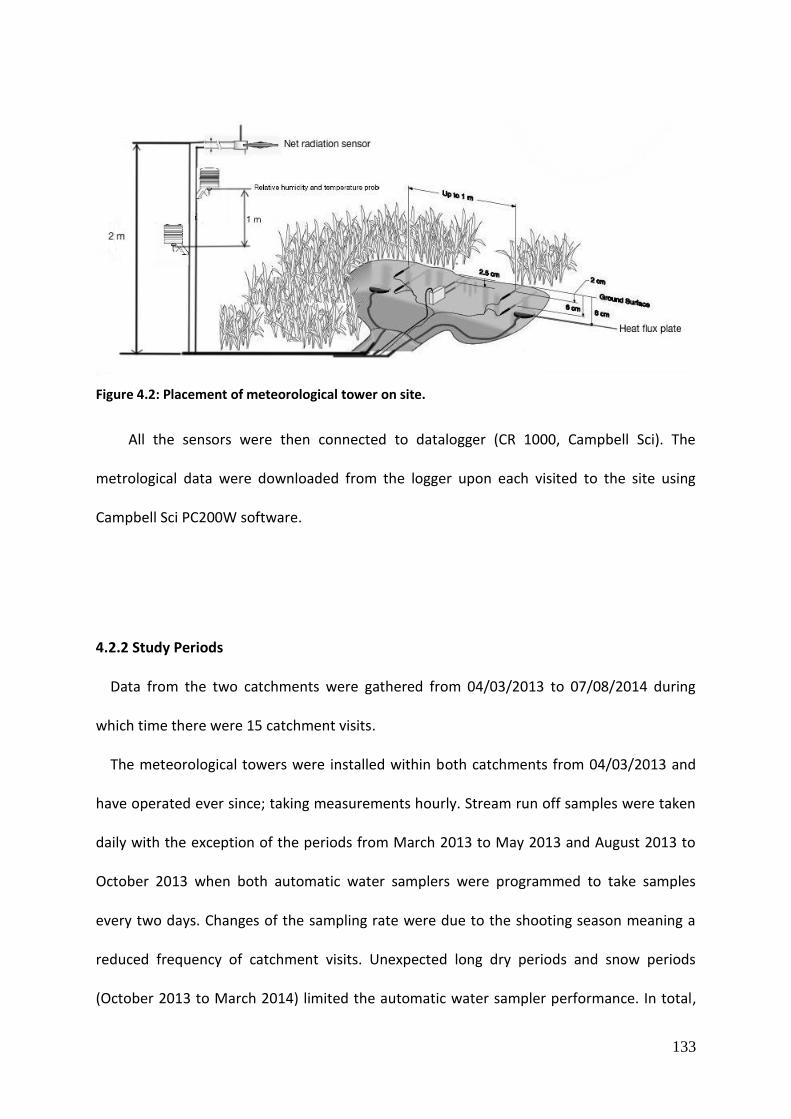
133

All the sensors were then connected to datalogger (CR 1000, Campbell Sci). The

metrological data were downloaded from the logger upon each visited to the site using

Campbell Sci PC200W software.

4.2.2 Study Periods

Data from the two catchments were gathered from 04/03/2013 to 07/08/2014 during

which time there were 15 catchment visits.

The meteorological towers were installed within both catchments from 04/03/2013 and

have operated ever since; taking measurements hourly. Stream run off samples were taken

daily with the exception of the periods from March 2013 to May 2013 and August 2013 to

October 2013 when both automatic water samplers were programmed to take samples

every two days. Changes of the sampling rate were due to the shooting season meaning a

reduced frequency of catchment visits. Unexpected long dry periods and snow periods

(October 2013 to March 2014) limited the automatic water sampler performance. In total,

Figure 4.2: Placement of meteorological tower on site.

134

there were 130 days of samples from the automatic water sampler for the control

catchment and 190 days of sampling for the experimental catchment. In addition to the run

off samples, spot samples were taken tracing the top of the gully to the main stream

channel on both catchments. Effectively, 8 out of 15 visits to the catchments were chosen to

take the spot samples.

4.2.3 Meteorological data

Initially, two micro-meteorological towers were constructed in the experimental and

control catchments. During the experimental period hourly recordings were recorded on the

tower on the experimental catchment. The tower on the control catchment has also been

recording data hourly and was functioning for 291 days out of the 386 days of the total

study period. The tower in the control catchment was set to record: temperature, humidity,

net radiation and water table. However, the height of meteorological tower in the control

catchment and the reflections of the solar panel raised the concerns from the game keeper

of the site, and eventually the net radiation and relative humidity probe along with tower

above the surface were removed under the request of the land management from

31/7/2013. After this date, only soil temperature, air temperature and water table changes

were monitored on the control catchment. The water evaporation was assessed through the

meteorological data, where net radiation, relative humidity and soil heat flux, and

evaporation were unified by the Bowen ratio (Romano and Giudici, 2009). The energy

balance can be written as:

𝑹𝒏 = 𝝆𝝀𝑬 + 𝑯 + 𝑮 (4.1)

135

With Rn : net radiation (W/m2), ρλE: latent heat flux (W/m2), ρ : density of water (kg/m3), λ:

latent heat of evaporation (J/kg), E: evaporation (mm/d), H: sensible heat flux (W/m2), G:

ground heat flux (W/m2).

The Bowen ration can be written as:

𝜷 = 𝑯

𝝆𝝀𝑬 = 𝜸

(𝑻𝟐−𝑻𝟏)

(𝒆𝒂,𝟐 − 𝒆𝒂,𝟏) (4.2)

With β: Bowen ration (-), γ: psychrometric constant (kPa/ ℃), T1: temperature at height z1

(℃), T2: temperature at height z2 (℃), ea,1: vapor pressure at height z1 (kPa), ea,2: vapor

pressure at height z2 (kPa).

By unifying equations 4.1 and 4.2, the evaporation can be written as:

𝑬 = (𝑹𝒏 − 𝑮)

𝝆𝝀 ( 𝟏+ 𝜷) (4.3)

To determine the evaporation in this way, it is necessary to measure the temperature and

relative humidity (Rh) at least at 2 heights. The relative humidity is determined by the

relation:

𝑹𝒉 = 𝒆𝒂 (𝑻𝒂)

𝒆𝒔 (𝑻𝒂) (4.4)

Where es (Ta) is the saturation vapor pressure at the current air temperature Ta.

Saturation vapor pressure (kPa) is a function of the temperature T (℃) and is expressed in

the formula:

136

𝒆𝒔 (𝑻𝒂) = 𝟎. 𝟔𝟏 𝒆𝒙𝒑 ( 𝟏𝟕.𝟑 𝑻

𝟐𝟑𝟕 + 𝑻 ) (4.5)

Thus, equation 1.3 can be transposed as follow:

𝑬 =(𝑹𝒏 − 𝑮)

𝝆𝝀⎨𝟏+ 𝜸(𝑻𝟐−𝑻𝟏)

𝟎.𝟔𝟏𝒉[𝒆𝒙𝒑 (𝟏𝟕.𝟑 𝑻𝟐

(𝟐𝟑𝟕 + 𝑻𝟐))−𝒆𝒙𝒑 (

𝟏𝟕.𝟑 𝑻𝟏(𝟐𝟑𝟕 + 𝑻𝟏)

] ⎬

(4.6)

Because of the meteorological tower in the control catchment was taken down during

the study, different approaches were used to calculate the water balance from control and

experimental data. The evaporation from the experimental catchment was calculated from

the Bowen ratio (Equation 4.6). Water balance was set to help elucidate flow pathways

especially considering the ephemeral nature of the streams in the study catchments. Lack of

evaporation data from the control catchment makes water balance from both incomparable

to each other. The water table variances of individual days of both catchments were then

used in the later statistical analysis as the water balance variable. The water table was

measured in the dipwells using pressure transducers to sense the depth of the water. The

transducers were programmed to take measurements hourly. A daily average water depth

was then calculated and used in the statistical analysis (referred to as water table from here

on). Similar to the events analysis conducted in Chapter 3, the rainfall factor was

characterised by its total daily rainfall (referred as total rainfall from here on). The pre-

existing moisture condition of the ground on to which any precipitation falls was assessed

by the total rainfall 24 hours prior to the start of the daily measurement of rainfall (referred

as antecedent rainfall from here on).

137

4.2.4 Runoff and spot sample data

Two automatic water samples were installed one each on the gullies draining the control

and experimental catchments. Due to the low occurrence of sampling by the auto-samplers,

a program of additional sampling was undertaken. On the basis that water from the study

catchments was not leaving via the monitored gullies the water must be draining vertically

through the soil profile, we started sampling the spring lines downslope of each study

catchment – this resulted in 93 spot samples being taken during the study period.

Furthermore, a total of 36 dipwells were installed in the experimental catchment in a

transect perpendicular to the natural stream (referred as runoff traps). Two small holes

were drilled opposite each other on the side of each trap. The two holes are approximately

30 cm up from the bottom side of the trap. Each runoff trap was placed the position (Figure

4.3) to make the small holes face perpendicular to the stream too. Thus any soil water

running perpendicularly towards the stream would have been trapped into the well. Due to

sampling point

Figure 4.3: the placement of runoff traps in experimental catchment

138

the hard sediment rock on both side of the control catchment, the runoff traps were only

applied in the experimental catchment.

4.2.5 Sample analysis

The water samples were analyzed in the laboratory for pH, conductivity, absorbance

and DOC concentration. The measurement of DOC concentration was by the colorimetric

method of Bartlett and Ross (1988). Sample absorbance was measured at 400, 465 and 665

nm using an UV/VIS spectrophotometer. Various studies have demonstrated a strong

correlation between absorbance of a sample at 400nm and the concentration of humic

matter (Korshin et al., 1997; Bertilsson and Tranvik, 2000). E4/E6 ratio is wildey used as a

measure of humification being the ratio of humic acids to fulvic acids (Anderson et al., 1981;

Wallage et al., 2006). The E4/E6 ratio was then calculated by using absorbance

measurements at 465 and 665 nm of the samples. During the study, the list of analyses was

expanded to include anions: fluoride (F), bromide (Br), chloride (Cl), nitrate (NO3),

phosphate (PO) and sulphate (SO4). The anion data were used in principal component

analysis (PCA) techniques to investigate the mixing of different waters in the system and to

establish the changes of chemical tracers through the stream thus further indicating the

potential changes in flowpaths through the study catchments (Worrall et al., 2003). Anion

analysis was performed by ion chromatography (IC). A Metrohm 761 compact-IC to an 813

Compact auto-sampler was used. Standards of 1.25, 2.5, 5 and 10 mg/l were used to create

linear calibration curve with samples. Two blank run were used before and after each the

standards. An eluent solution of sodium carbonate and sodium hydrogen carbonate were

used to maintain a stable baseline.

139

4.2.6 Statistical analysis

The revegetation effects on DOC concentration and water colour was assessed by

relative DOC and relative water colour. Both the relative DOC and relative water colour

were calculated as the DOC concentration and water colour from the experimental

catchment relative to that in the control catchment for the same month. No water samples

or the meteorological data were taken prior to the start of experiment and, therefore, the

relative data was not used to assess whether the DOC concentrations or water colour are

different between the study catchments but whether the DOC and water colour in the

stream runoff in the experimental catchment declines relative to the control catchment

with time. Due to the differences between control and experimental catchments, i.e.

different dry or wetness conditions of the catchment; different snow melting conditions on

different catchments, the auto sampler in experimental catchment was not always

collecting runoff samples simultaneously within the control catchment. It was only possible

to calculate relative data for 87 days, as a result.

Statistical analysis was applied to the experimental data to assess the benefit of

revegetation on DOC or water balance. Two sets of data both include runoff data and

meteorological data in statistical analysis, one is based on the DOC variation (Set 1), the

other one is based on the relative DOC variation (Set 2). Set 1 data contains the DOC

concentration, water colour, pH, conductivity, ion chromatography, antecedent rainfall

which was calculated from the previous 24 hours meteorological records, and the water

balance of the day. Set 2 data was the relative DOC concentration, month and antecedent

rainfall.

Analysis of variances (ANOVA) was applied to the set 1 data to identify the dominant

variables in DOC concentration changes in the control and experimental catchments.

140

Therefore, DOC concentrations from both catchments were assessed with following factors:

month, catchment and spot. The month factor have 12 levels representing the 12 months of

a year, catchment factor has 2 levels, one for each catchment. Spot factor has two levels,

spot sample or not spot sample. Besides the factors applied on the ANOVA, pH,

conductivity, antecedent rainfall, evaporation and average temperature of the day were

considered as covariates. Set 2 data assessed all stream runoff data from the experimental

catchment relative to control catchment over the monthly changes to identify the

revegetation effects. An ANOVA was applied on set 2 data with the same factors and

covariates used in ANOVA of set 1. In both the ANOVA performed on set 1 and set 2 data,

the proportion of variance explained by a factor or covariate was calculated by using the ω2

method by Vaughan and Corballis (1969), hence any factors or covariates having a

probability larger than 95% of not being zero were considered as significant.

Principal component analysis (PCA) was used to understand changes in flow

pathways between catchments. The compilation of DOC, water colour, pH and conductivity

from set 1 were used in PCA to identify common evolution to stream from soil water. Similar

to chapter 3, principal components (PCs) with eigenvalues greater than 1 and the first PC

with an eigenvalue smaller than 1 were selected for further inspection. The process of

selecting PCs for further inspection is sometime an arbitrary decision (Chatfield and Collins,

1981). The eigenvalue of the correlation matrix which PCA is based on the sum of the

diagonal terms, thus the eigenvalue of PCs is equivalent to the number of variables in the

original dataset. The rule for choosing PCs can then be explained as the chosen PCs

explained more variance than any of the original variables. The parameters applied in PCA

all retained different units. Since principal components are calculated from the covariance

matrix of the variables, the variables are required to ensure equal weight in the PCA. By z

141

transforming all the variables considered in the PCA, all the variables are brought to the

same scale (details see chapter 3). As PC scores for one component were plotted against

another, the distribution of those score would form clear patterns or easily assessed end-

members. The end-members were identified through the plots and the end-member data

was reached by comparing scores from the two PCs which formed the plots. The analysis of

end-members (EMMA) are commonly used in the analysis of mixing sourced water analysis

(Christophersen and Hooper 1992) to help to identify the different source of water. Worrall

et al. (2003) illustrated the use of PCA for mixing analysis combined with end-member

analysis in an upland peat catchment by comparing samples along potential flow paths from

precipitation and ground water, through soil water to streamflow. A further PCA was

performed including the anion data. The variables used in PCA were: DOC, water colour, pH

and conductivity, water balance; and the anion data from both catchments (Anion PCA). The

extension of variables of anion data from set 1 was applied to identify the potential effects

of flow path changes, i.e. the dilution from the flow path changes. End-member analysis and

ANOVA of PCA was applied to the Anion PCA too. The statistical analysis was to help

elucidate flow pathways, especially considering the important ephemeral nature of the

streams in the study catchments. The water balance on both the control and experimental

catchments should also be included in the previous statistical analysis. After initial

assessment of the PCs some were subsequently subjected to an ANOVA following the same

methods stated in this section. The principal components applied in ANOVA were the first

two components as combined two components usually represented about 50% of the

original data variance. The ANOVA was applied on these components to access whether

these values vary significantly due to revegetation. The factor included in this ANOVA

includes: catchment, month and spot. The covariates in the ANOVA were: pH, conductivity.

142

4.3. Results and Discussion

4.3.1 DOC concentration

Assessing all stream runoff and spot samples during the experiment periods shows that

DOC concentration increased from 31.65 mg C/l to 41.68 mg C/l between control and

experimental catchments in all runoff samples (Figure 4.4). Comparisons of DOC

concentrations were made between the two catchments in the two different water sample

types: stream water runoff collected by auto sampler (referred as runoff) and soil water

collected along the stream track (referred to as spot). Results shows that DOC concentration

differences between catchments were smaller in spot samples than in runoff samples. The

median DOC concentration was 33.65 mg C/l compared to 44.68 mg C/l in runoff samples

and median DOC concentration was from 35.60 mg C/l compared to 35.89 mg C/l in spot

samples (Figure 4.5). There are two things that should be noted. First, sampling rates of

runoff samples in two catchments were different, sampling rates in the experimental

catchment were 15.6% higher than in the control catchment. Second, the spot samples

were collected on both catchments per visit to the site, and therefore there is a much

smaller contrast between sampling rates of the two catchments, with the sampling rate of

the experimental catchment was only 3.5% higher than that of control catchment.

143

EXPERIMENTALCONTROL

80

70

60

50

40

30

20

10

0

DO

C c

on

ce

ntr

ati

on

( m

g c

/l)

Figure 4.4: Boxplots of DOC concentration in both catchments. The box represents the inter- quartile range; the whiskers represent the range of the data; and the horizontal bar represents the median value.

catchemnt

spotrunoff

EXPERIMENTALCONTROLEXPERIMENTALCONTROL

80

70

60

50

40

30

20

10

0

DO

C c

ocn

en

tra

tio

n (

mg

c/

l)

Figure 4.5: DOC concentrations of runoff and spot samples from both catchments.

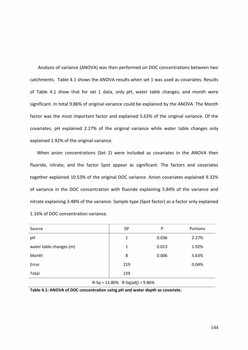
144

Analysis of variance (ANOVA) was then performed on DOC concentrations between two

catchments. Table 4.1 shows the ANOVA results when set 1 was used as covariates. Results

of Table 4.1 show that for set 1 data, only pH, water table changes, and month were

significant. In total 9.86% of original variance could be explained by the ANOVA. The Month

factor was the most important factor and explained 5.63% of the original variance. Of the

covariates, pH explained 2.27% of the original variance while water table changes only

explained 1.92% of the original variance.

When anion concentrations (Set 2) were included as covariates in the ANOVA then

fluoride, nitrate, and the factor Spot appear as significant. The factors and covariates

together explained 10.53% of the original DOC variance. Anion covariates explained 9.32%

of variance in the DOC concentration with fluoride explaining 5.84% of the variance and

nitrate explaining 3.48% of the variance. Sample type (Spot factor) as a factor only explained

1.16% of DOC concentration variance.

Table 4.1: ANOVA of DOC concentration using pH and water depth as covariate.

Source DF P Portions

pH 1 0.036 2.27%

water table changes (m) 1 0.013 1.92%

Month 8 0.006 5.63%

Error 219 0.04%

Total 229

R-Sq = 13.80% R-Sq(adj) = 9.86%

145

Source DF P Portions

Fluoride (as F) 1 <0.001 5.84%

Nitrate (as N) 1 0.004 3.48%

Sample type 1 0.058 1.16%

Error 198 0.04%

Total 201

R-Sq = 11.87% R-Sq(adj) = 10.53%

Table 4.2: ANOVA of DOC concentration using anion concentrations as covariates.

Total rainfall on the day, catchment and spot as factors were not found to be

significant when considered in the ANOVA (Table 4.1). The month factor shows that

seasonal changes were more influential than other factors. The water table changes, rather

than total rainfall of the day, as a significant factor to DOC variance may suggest influences

of water balance on DOC concentration. However, whether the water table changes are due

to the revegetation is not clear and will be assessed below. The low proportion of the

variance explained by the ANOVA (Table 4.1) may be caused by the failure of runoff

sampling. i.e. the extreme conditions during the experimental periods caused low sampling

rates in both catchments and the auto-samplers would only take samples when peak flow

events occurred. The difference between spot and runoff samples is a significant factor,

albeit only explaining a small variance in Table 4.2. The significant variances of anion

covariates from Table 4.2 may hint at a different source of water or the flow path changes

that may contribute to the DOC changes between the two catchments. Further

identification of the source of water or flow path changes may require the principal

component analysis (PCA) of the available data. The lack of pre-experimental period data

means that the analysis should be focused on the DOC concentration changes and water

colour changes from experimental catchment relative to control catchment over time.

146

Overall, the analysis of variances did not observe any direct influence from revegetation

upon DOC concentration.

4.3.2 Relative DOC concentration

Relative DOC concentration change did not appear to show an increase or decrease

over time (Figure 4.6). In between late winter to early spring (January to March), DOC

concentrations increased by an average of 7.8% per month relative to the control. Early

winter periods (October to December), however, showed the rise and fall of relative DOC

concentration between the three months. There is no clear trend in the relative DOC

changes over the months that could be shown in Figure 4.6, as the relative DOC neither

increases or decreases over the months. ANOVA was once again applied on the relative DOC

concentrations from both catchments. However, none of the factors or covariates were

found to be significant in this analysis. This result suggests that revegation was not

successful in decreasing the DOC concentration.

147

121110431

3

2

1

0

-1

Month

rela

tiv

e D

OC

Figure 4.6: Relative DOC concentration changes over months.

4.3.3 Water colour

Water colour of both catchments was measured through the sample absorbance

reading at 400 nm and E4/E6 ratios. Boxplots of both absorbance and the E4\E6 ratio show

higher water color on samples collected from the experimental catchment than the samples

collected from the control catchment (Figures 4.7 and 4.8). The UV-Vis absorbance at 400

nm shows a median value of 0.125 for the control catchment compared to the median value

of 0.181 for the experimental catchment. The E4/E6 ratios showed a contrast of ratios from

0.720 to 3.261 moving from control to the experimental catchment. The increases of the

absorbance and ratio from control to experimental catchment indicated there are more

humic compounds being detected from samples taken from the experimental catchment

than from the control catchment. The boxplots of the 400 nm absorbance and the E4/E6

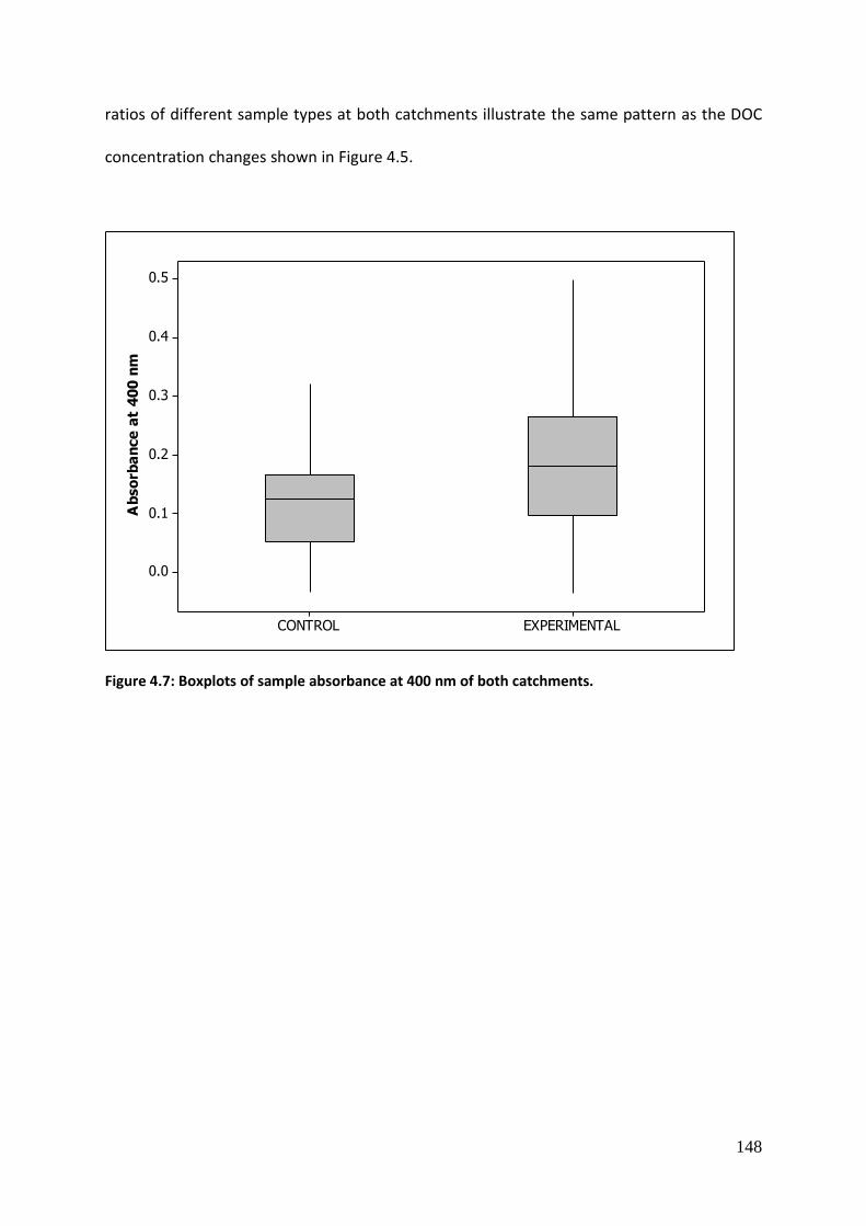
148

ratios of different sample types at both catchments illustrate the same pattern as the DOC

concentration changes shown in Figure 4.5.

EXPERIMENTALCONTROL

0.5

0.4

0.3

0.2

0.1

0.0

Ab

so

rba

nce

at

40

0 n

m

Figure 4.7: Boxplots of sample absorbance at 400 nm of both catchments.

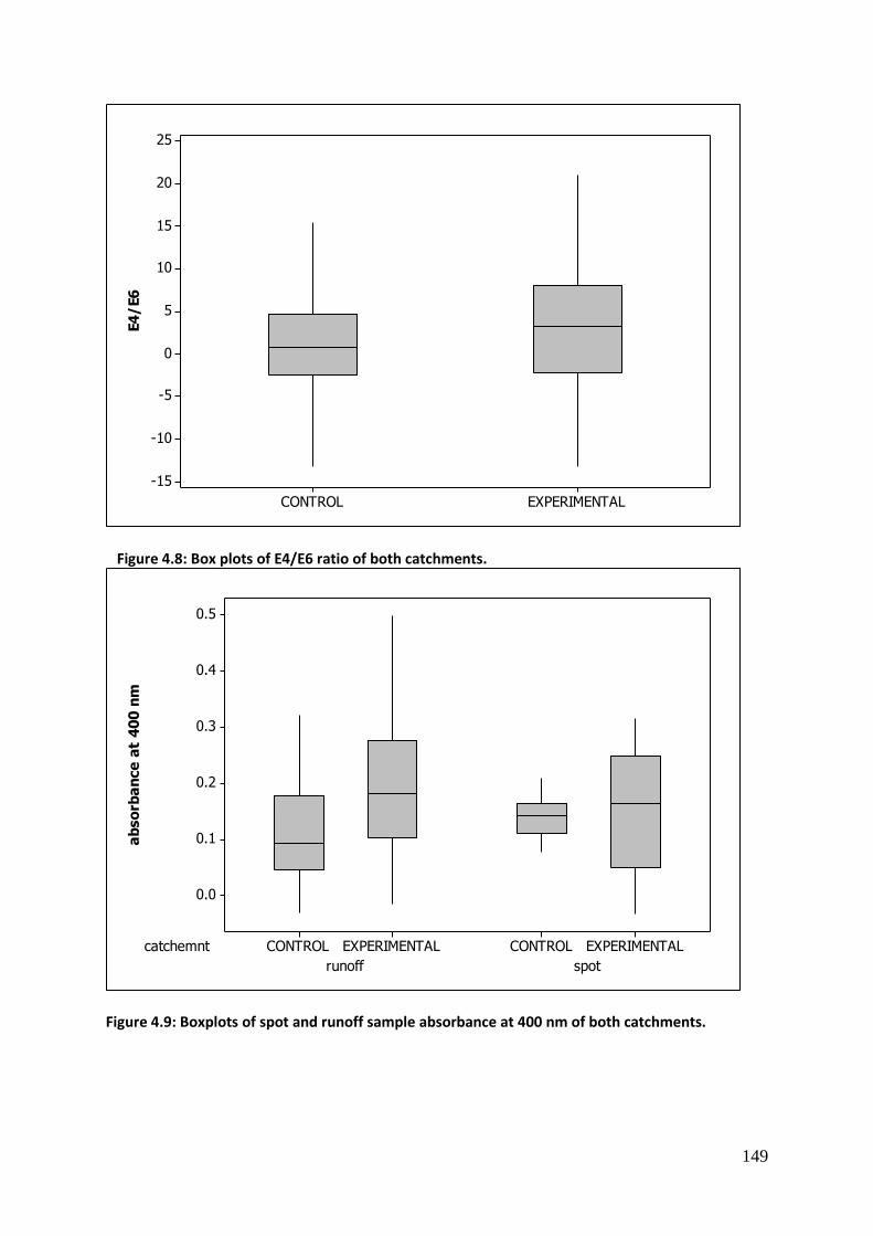
149

EXPERIMENTALCONTROL

25

20

15

10

5

0

-5

-10

-15

E4

/E6

Figure 4.8: Box plots of E4/E6 ratio of both catchments.

catchemnt

spotrunoff

EXPERIMENTALCONTROLEXPERIMENTALCONTROL

0.5

0.4

0.3

0.2

0.1

0.0

ab

so

rba

nce

at

40

0 n

m

Figure 4.9: Boxplots of spot and runoff sample absorbance at 400 nm of both catchments.

150

catchemnt

spotrunoff

EXPERIMENTALCONTROLEXPERIMENTALCONTROL

25

20

15

10

5

0

-5

-10

-15

E4

/E6

Figure 4.10: E4/E6 of runoff and spot samples from both catchments.

Both the 400 nm absorbance and E4/E6 ratio in runoff samples have larger median

values in the experimental catchment than in the control catchment. There was a 92.5%

increase on the median values of the concentration in runoff samples from control to

experimental catchment, and the median value of E4/E6 ratio in experimental catchment

was approximately 5.34 times higher than the value for the control catchment. The changes

between catchments on spot samples is much smaller than that seen for the runoff samples,

with a 16.2% increase from the control catchment to the experimental catchment on the

400 nm absorbance reading and a 35.2% increase of the same kind in E4/E6 ratios.

Following the observation of the DOC concentration changes in section 3.1, the differences

of water color between two kinds of water samples may also illustrate the influence of the

different sampling rates between two kinds of soil samples. While the runoff sample rates

suffered largely by extreme dry or frozen conditions of the land and the failure of the

151

autosamples, the differences of spot sampling rates are relatively smaller than that of runoff

samples. Hence, the water color changes between catchment may not be as severe as

Figure 4.7 and Figure 4.8 appear to suggest. The further test of influence with this sample

type differences on water color could be performed on ANOVAs on the 400 nm absorbance

where sample types was used as an factor alongside with other factors such as month,

catchment, antecedent rainfall and covariance such as pH, conductivity and anion data. A

similar test could also be performed on the E4/E6 ratios too.

Source DF P Portion

pH 1 <0.001 20.22%

Catchment 1 <0.001 7.52%

Sample types 1 0.037 0.01%

Month 9 <0.001 27.02%

Antecedent rainfall 85 <0.001 11.16%

Error 161

0.02%

Total 258

65.96%

S = 0.0603560 R-Sq = 78.81% R-Sq(adj) = 66.04%

Table 4.3: ANOVA of absorbance (400 nm) when pH and conductivity are applied as covariates.

.

Source DF P Portion

pH 1 <0.001 26.67%

Chloride (as Cl) 1 <0.001 6.47%

Nitrate (as N)_1 1 0.002 6.74%

Conductivity 1 <0.001 1.72%

Water table changes (m) 1 0.003 1.99%

Catchment 1 <0.001 9.60%

Sample types 1 0.002 0.02%

Month 9 <0.001 18.36%

Error 166

0.11%

Total 182 S = 0.0510327 R-Sq = 74.18% R-Sq(adj) = 71.69%

Table 4.4: ANOVA of absorbance (400 nm) when anion data were included as covariates.

152

When pH and conductivity were included in the ANOVA of absorbance at 400nm (Table

4.3), the results show all factors included in the ANOVA were significant in explaining the

variance of absorbance. Of the two covariates, only pH was found to significant and

explained 20.22% of the original variance in the absorbance. Among 4 significant factors,

Month explained the most variance in the absorbance changes (27.02%), followed by

antecedent rainfall (11.16%) and then catchment (7.52%), and the sample type explained

the least variance of the absorbance (0.01%). In total, the factor and covariates explained

66.04% of the original variance in the absorbance data.

In the ANOVA of absorbance at 400 nm with the anion data used as covariates (Table

4.4), month (explained 18.36% variances), catchment (9.6% of the variances) and sample

types (0.02%) were found to be the significant factors. Significant covariates were: pH

(26.67%), chloride (6.47%), nitrate (6.74%), conductivity (1.72%) and water table changes

(1.99%). Variates combined the factors and covariates together explained 71.69% of the

variance of the absorbance changes.

Table 4.5: ANOVA of E4/E6 ratio.

When the same ANOVA was applied to the E4/E6 ratios, the results (Table 4.5) of ANOVA

found only water table was the significant factor, contributing 24.2% of the E4/E6 ratio

variance.

Results of ANOVA on the absorbance indicates that the seasonal change is the most

important factor on the absorbance variance. The catchment was a significant factor

Source DF P

Water balance 132 0.004

Error 119 Total 251 S = 15.8965 R-Sq = 64.06% R-Sq(adj) = 24.20%

153

indicating that the revegetation effects are the dominant feature between catchment

differences. Although the sample types were identified as a significant factor, however the

small proportion it contributed to the absorbance indicates the different sample types may

not play an important role (Figure 4.9 and 4.10). Antecedent rainfall as a significant

covariate disappeared when anion data were included in the ANOVA of absorbance, while

the pH was still a significant covariate. The changes of the antecedent rainfall were replaced

by various anions. The anion factor combined with the relative high proportion of pH

contribution to the whole absorbance variance may indicate changes of flow path or

changes in source water mixing.

The ANOVA of E4/E6 ratio also indicated the water table changes were the only factor

contributed to the changes in the proportion of humic compounds. As the catchment,

sample types and month are all ruled out as potential influences on the humic compound

changes, the water table changes therefore may also point to the potential influence of

revegetation on the humic compound characteristics.

4.3.4 Relative water colour

The relative water colour was assessed through the samples absorbance at the

wavelength of 400 nm for the experimental catchment relative to the control catchment

and the E4/E6 ratio of the experimental catchment relative to control catchment over the

months (Figures 4.11 and 4.12). Both the relative absorbance (400 nm) and relative E4/E6

ratios showed no clear changes between different months. By comparing the two Figures

(Figures 4.11 and 4.12), the observed change in the relative absorbance is reversed when

compared to the change in the E4/E6 ratios, i.e., the median relative absorbance changes

increased from 0.28 (January) to 3.8 (March) and decreased to 0.12 (April) while the relative

154

ratios was decreased from 0.05 (January) to -4.6 (March) and then increased to 0.014

between January and April. The changes between the months in both Figure 4.11 and Figure

4.12 were also observed to be getting smaller with time. Changes in Figures 4.11 and 4.12

indicate the reverse relationship between the water colour and less humic compounds of

the samples collected for the site, i.e. the high water colour observed over months is

associated with having less humic compounds in the sample.

ANOVA was used to analyses changes in both relative absorbance (ƛ=400 nm) and

relative E4/E6 ratio over the months. Month was used as a factor and antecedent total

rainfall was used as covariate in both ANOVA. In the ANOVA of relative absorbance, month

was found to be the only significant factor and explained 21.73% variance in the relative

absorbance changes. There were no significant factor or covariates found in the ANOVA of

the relative E4/E6 ratios. In the ANOVA of the relative absorbance, the monthly changes

were not associated with the precipitation as no interaction between Month factor and

antecedent rainfall total was observed. In fact, the antecedent rainfall was not found to be a

significant covariate at all in both the variance of relative absorbance and relative E4/E6

ratio changes indicates the month factor here in both ANOVA of relative absorbance and

relative E4/E6 ratio would represent influence other than that due to precipitation. The

seasonal changes observed in both Figures 4.11 and 4.12 may indicate that seasonal

variations are a consequence of revegetation. However, the low sampling rates over the

several months made the analysis ustruggle to reveal a clear trend of water color changes

over experimental periods. In terms of the result of ANOVA of relative E4/E6 ratio changes

no factor or covariate was found to be significant, and perhaps associated with the

hydrological changes i.e. the flow path changes during the peak flow events.

155

121110431

5.0

2.5

0.0

-2.5

-5.0

-7.5

-10.0

Month

rela

tiv

e a

bso

rba

nce

at

40

0 n

m

Figure 4.11: relative absorbance at 400 nm over months, where there was only one reading available in March. where 1 stand for Jan, ect.

121110431

20

15

10

5

0

-5

-10

Month

rela

tiv

e E

4/

E6

ra

tio

Figure 4.12: Relative E4/E6 ratio over months, where there was only one reading available in March. where 1 stand for Jan, ect.

156

4.4 Water balance

4.4.1 Water table

Observations of water table depth have been made during the study periods with a total of

715 observations being recorded. In general, the experimental catchment observed a small

mean increase of 0.16 m of the daily average water table depth to the control catchment

(Figure 4.13) over the study period. An ANOVA was performed on the water table data from

the site and it was found that month, catchment and antecedent rainfall total were

significant, and together explained 56.81% of the original variance (Table 4.6). The Month

factor explained the majority of the variance in the data and the antecedent rainfall total

explained the least. There were no significant interactions between the factors. Although

the ANOVA indicates the catchment factor as significant and this is manifest as a higher

water table in experimental catchment, the impact of catchment was uncertain due to the

lack of the pre-vegetation periods data.

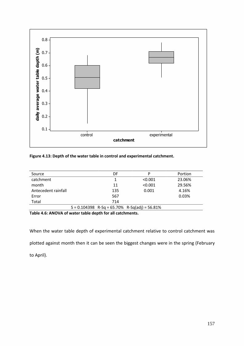
157

experimentalcontrol

0.8

0.7

0.6

0.5

0.4

0.3

0.2

0.1

catchment

da

ily a

ve

rag

e w

ate

r ta

ble

da

pth

(m

)

Figure 4.13: Depth of the water table in control and experimental catchment.

Source DF P Portion

catchment 1 <0.001 23.06% month 11 <0.001 29.56% Antecedent rainfall 135 0.001 4.16% Error 567

0.03%

Total 714 S = 0.104398 R-Sq = 65.70% R-Sq(adj) = 56.81%

Table 4.6: ANOVA of water table depth for all catchments.

When the water table depth of experimental catchment relative to control catchment was

plotted against month then it can be seen the biggest changes were in the spring (February

to April).

158

12111098765432

4

3

2

1

0

month

rela

tiv

e d

aily

wa

ter

tab

le d

ep

th

Figure 4.14: relative water table depth over months, where January is marked as month 1 etc.

Relative daily water table depths between the months were observed (Figure 4.14). An

ANOVA of relative daily water table found only month as the significant factor at explaining

24.77% of the original variance. The antecedent rainfall was not found to be a significant

covariate to the relative water table depth indicating the changes of relative water table

depth were not driven by the change of antecedent rainfall.

The analysis of both water table depth in catchments and the relative water table depth

indicated the effects of revegetation on maintaining an higher water table depth in the

experimental catchment compared to the control catchment.

4.4.2 Evaporation

Since the meteorological tower was taken down at the end of July 2013, the evaporation

was calculated based on the experimental catchment. During experimental periods, the

159

experimental catchment observed an average of 6 mm / day evaporation. Figure 4.16 shows

the changes of daily evaporation rate over months.

1211109876543

30

20

10

0

-10

month

ev

ap

ora

rtio

n (

mm

/d

ay

)

Figure 4.15: Box plots of daily evaporation over months.

Figure 4.15 seems to show seasonal changes over the study periods. The median value

of daily evaporation was observed to increase from March (0.24 mm/day) to July

(17.27mm/day) and decrease from then to December (1.9 mm/day). Seasonal covariates

includes temperature and antecedent daily total daily rainfall as covariates, along with

month were used as factor for an ANOVA of daily evaporation. The results of ANOVA (Table

4.7) show month along with temperature explained 56.6% of data variances where

temperature as covariates explained 29.56% of the original variance and month as a factor

explained 26.95% of the original variance. Antecedent rainfall was not found to be a

160

significant factor. The interaction between month and daily average temperature was also

found not to be a significant factor.

Source DF P Portion of variances

Temperature 1 0 29.56%

month 9 0 26.95%

Error 280

1.30%

Total 290

S = 0.00541073 R-Sq = 58.09% R-Sq(adj) = 56.60%

Table 4.7: Results of ANOVA of daily evaporation in experimental catchment.

The seasonal changes observed in Figure 4.15 therefore are mainly controlled by

changes in the temperature, however, the changes between months are not due to the

variations in the antecedent rainfall. A significant month factor above and beyond that

explained by significant covariates may indicate changes of vegetation. In Figure 4.16, the

spring and summer show a relative low variation of evaporation with a monthly evaporation

difference of 40% during autumn and winter season with 190% monthly evaporation change

between months. However, the lack of comparison between control and experimental

evaporation make the effects of changes of revegetation hard to assess.

161

4.5 Principal components analysis of DOC

Variable PC1 PC2 PC3

Z pH 0.544 -0.185 0.063

Z conductivity -0.21 0.352 0.355

Z DOC 0.429 -0.394 0.203

Z E4/E6 0.038 -0.011 0.901

Z temperature 0.567 0.273 -0.103

Z antecedent rainfall -0.009 0.602 0.053

z water table changes 0.39 0.499 -0.055

Eigenvalue 1.8518 1.4844 1.0248

Proportion 26.50% 21.20% 14.60%

Cumulative 26.50% 47.70% 62.30%

Table 4.8: First three principal components of PCA . Where absolute loading values bigger than 0.400 were considered as dominate loadings and marked red.

Principal components analysis (PCA) was applied to understand the mixing of water

types and changes in flow path between the study catchments. There were three principal

components (PCs) selected during analysis. In total, these three PCs explained 62.3% of

variances in the data set (Table 4.8). Among three PCs, PC1 is dominated by significant

positive loadings of pH, DOC, and temperature. PC2 has high positive loadings for

antecedent rainfall and water table changes. PC3 has very high positive loadings for the

E4/E6 ratio which represents the DOC composition changes. From the different dominant

loadings of each principal component, PC1 can be seen as the influences of DOC changes

with the variances of pH and temperature, PC2 as the influence of hydrological changes, and

162

PC3 is the change of humic compounds. A comparison of PC1 and PC2 for all sample types is

shown below (Figure 4.16).

Figure 4.16: A comparison of PC1 and PC2 for all sample types.

The pattern of data suggests that the stream runoff water in both catchments has a

common end-member composition (Marked A, Figure 4.16) that in part reflects a dilution

trend of soil water samples (Marked B, Red line, Figure 4.16). A series of control spot

samples were gathered with events of decreasing DOC concentration and increasing total

rainfall could be identified (Marked D, green line, Figure 4.16). This green line is largely

made up of samples gathered on 31/07/13, where an event of highest water table changes

and high antecedent rainfall compared to other days for the rest of the spot samples was

163

collected. The separation between samples from 31/07/13 and the rest of the samples from

both catchments indicates the comparison of high peak flow and low flow events.

The stream runoff water evolves to one of the runoff samples (Marked C, Figure 4.17) with

low antecedent rainfall and water table changes. Comparing the two catchments suggests

no difference in the mechanism of DOC runoff. A series of ANOVA were chosen to access

the early observed different sample rate influence on DOC concentration changes (Section

3.1). Of the three principal components selected, only PC1 and PC3 had high loadings for the

DOC concentration. Thus the ANOVA were applied on PC1 and PC3. In the ANOVAs of PC1

were applied on each catchment using sample type (runoff or spot) as factor with pH and

conductivity as covariates. In the ANOVA of PC1 in the control catchment, sample type was

found to be a significant factor which explained 18.95 of PC1 variance. In the ANOVA of

experimental catchment, sample type was also found to be significant factor explaining only

2.12% of the PC1 variance. In the control catchment, DOC concentration of the spot

samples (median value of 35.6 mg C g/l in Figure 4.5) are higher than stream runoff samples

(Median value of 33.6 mg C g/l in Figure 4.5) but in the experimental catchment the

difference is reversed with spot samples having lower DOC concentration (Median value of

35.8 mg C g/l in Figure 4.5) than stream runoff samples (Median value of 44.6 mg C g/l in

Figure 4.5). When pH and conductivity were included as covariates in the ANOVA of PC1,

sample type was still observed as a significant factor with P value less than 0.001 and

explained 25.9% of the original variance in the control catchment, explaining 6.36% of the

original variance. ANOVA of PC1 for the two catchments comparing their respective stream

runoff and spot samples shows that there was a significant interaction with the difference

between stream runoff and spot samples being different between the experimental and

164

control catchment. However, for the ANOVA of PC3, which stands for the water colour

changes, the sample type was not a significant factor in either of the catchments. The

changes of the water colour were not due to the interaction with the difference between

sample type being different in the two catchments indicating possible DOC composition

changes or flow path changes.

4.6 Principal components analysis including anion data

The PCA of the DOC, water colour, antecedent rainfall, water table changes, pH and

conductivity give different features when the anion data from both catchments were

included. There were 6 anion variates included in the PCA. There were fluoride, chloride,

nitrate, sulphate, and nitrite. All the variates have been z transformed. There were four

principal components chosen from the PCA (Table 4.9) and these 4 PCs explained 65.6% of

variance of the data included in the analysis. Among the four PCs, the first component (PC1)

and second component (PC2) together explained about half of the original variance in the

data (44.6%). First principal component (PC1) is dominated by the positive loadings of nitrite

(loading of 0.437) and nitrate (loading of 0.450), second principal component is dominated

by negative loading for chloride (loading s of -0.572) and conductivity (loading of -0.60).

Third principal components have the distinct loading for nitrate (negative loading of -0.43)

and pH (positive loading of 0.554). Unlike the first three principal components that were

dominated by variation in anion concentrations, the fourth principal component (PC4) was

dominated by variation in DOC (loading of 0.612) and fluoride (loading of 0.592).

165

Variable PC1 PC2 PC3 PC4

Z Fluoride (as F) 0.166 -0.145 -0.116 0.592

Z Chloride (as Cl) 0.222 -0.572 0.018 -0.085

Z Nitrate (as N) 0.361 0.046 -0.430 -0.193

Z Sulphate (as S) 0.424 -0.223 0.062 0.019

Z Nitrate (as NO2-) 0.437 0.282 -0.153 -0.166

Z Nitrate (as NO3-) 0.450 0.259 -0.193 -0.172

Z pH 0.227 -0.020 0.554 0.059

Z Conductivity 0.106 -0.600 -0.085 -0.020

Z DOC 0.035 0.021 -0.403 0.612

Z E4/E6 -0.006 0.036 -0.049 -0.015

Z PTemp_C_Avg 0.253 0.227 0.403 0.270

Z Antecedent rainfell 0.146 -0.173 0.156 -0.205

Z water table changes 0.262 0.097 0.267 0.231

Proportion 27.70% 16.90% 11.30% 9.70%

Cumulative 27.70% 44.60% 55.90% 65.60%

Table 4.9: First four principal components selected by PCA including anion data. Where absolute loading values bigger than 0.400 were considered as dominate loadings and marked red.

The pattern of Figure 4.18 and its end-members (E-F-G) are quite distinct from that

of Figure 4.17. Plot of PC1 against PC2 in PCA including anion data (Figure 4.17) suggests

that the runoff water and spot samples in both catchments are sourced from a common

end-member (Marked E in Figure 4.17). The majority of samples from the experimental

catchment appear to evolve in two opposite directions (Marked F and G in Figure 4.17)

which dominated by stream runoff and spot samples respectively. Stream runoff of

166

experimental catchment evolves from samples composted by low concentrations of nitrite,

nitrate, chloride and low conductivity to samples containing high concentrations nitrite,

nitrate, conductivity and chloride. Compared to runoff samples from the experimental

catchment, spot samples are changing from the same composition of low nitrite, nitrate,

chloride concentration and low conductivity to the high nitrite, nitrate concentration but

lower conductivity and chloride composition. Comparing control to experimental

catchments indicates no clear compositional changes of the samples. Two sets of ANOVAs

were applied on first two principal components (PC1 and PC2).

Figure 4.17: A comparison of PC1 and PC2 for all sample types based on anion data.

Results of two sets of ANOVA using sample type (stream runoff and spot samples) as

a factor between the two catchments respectively suggesting that the difference between

samples types in the control catchment was not significant for either PCs while the sample

167

type was a significant factor (p<0.001) for PC2 (the factor explained 11.9% of variance of

PC2) but not a significant factor for PC1 in the experimental catchment. As the difference of

sample type reflects mainly in the different sampling rates, the different pattern (line EG

and EF in Figure 4.17) indicate the soil runoff water suffered by the change of severe

weather condition dominated sample rate variances and thus concentration changes of

nitrate and nitrite (Pattern of EF) were linked to the experimental runoff samples. The trend

E-G linked concentration changes of chloride and change of conductivity to experimental

spot sample sampling rates which are less affected by weather conditions. Therefore, the

pattern changes on Figure 4.17 reflect the composition changes of water samples. Beside

PC1 and PC2 in the PCA of anions (Table 4.9), the fourth principal component (PC4) is the

only component dominated by the loading of the DOC concentration (positive loading of

0.621 in Table 4.9). As all first three components represent one composition combination of

data set 2 been analyzed, each of three components is plotted against the PC 4 to identify

the possible relationship between DOC and each composition albeit PC4 only represents

9.75% of variance of data.

168

Figure 4.18: A comparison of PC1 and PC4 of all sample types based on anion data.

A mix of all type of samples in both catchments of Figure 4.18 suggests no DOC composition

changes on nitrite and nitrate level at all types water of both catchments albeit there is a

clear separation of control spot samples (Red dots of Figure 4.18). The control spot samples

towards the negative end of PC1 on Figure 4.18 were from the 31/07/13 which has already

been identified above as an event marked out by the high antecedent rainfall. The

separation of control spot sample is most likely to be caused by the hydrological difference

between the days upon which spot samples were taken. The apparent difference in the

variance of the spot samples with respect to nitrite and nitrate composition from the two

catchments may be caused by the catchment difference, but may primarily suggest the

experimental spot sample are less sensitive to the hydrological change. Patterns visible in

Figure 4.19 suggested the spot samples’ DOC is less variable with respect to conductivity

169

and chloride, whereas the runoff samples’ DOC is more variable with changes in

conductivity and chloride. In fact, the decrease of DOC on Figure 4.19 (Marked Green and

Red lines) comes with the rapid changes of conductivity and chloride. Figure 4.20 shows the

variance of pH and nitrate of samples from control catchment while the spot samples and

runoff samples of the experimental catchment evolve to the opposite end of the pH and

nitrate variance.

Figure 4.19: A comparison of PC2 and PC4 of all sample types based on data set 2.

Comparisons of all three plots (Figures 4.18 to 4.20) suggest the DOC composition changes

between catchments. The runoff samples and upper stream DOC composition are

associated with the variances of nitrite, nitrate, conductivity and chloride. The control

catchment DOC is less altered by the variance of pH and nitrate, but the experimental

catchment DOC varies with the changes of pH and nitrate. The analysis of PC1 vs PC2 have

170

illustrated the DOC removal on the experimental catchment, the analysis of DOC

compositions here further indicates the removal of DOC may be due to flow path changes.

Figure 4.20: A comparison of PC3 and PC4 of all sample types based on data set 2.

The relative DOC changes of an earlier study contradict with the PCA results, where no

linear relationship of relative DOC between months was observed. The observation of the

relative DOC leads to the assumption that DOC removal observed may not be because of the

revegetation. However, results of the relative water table changes over the months suggest

that the revegetation indeed leads to the stable water table. It should be noted that the lack

of comparable data across different months leads to the separation in Figure 4.12 to form 2

sections with spring and winter. The noticeable stable relative water table may just reflect

the frozen water table during low temperature and thereby the DOC changes would most

unlikely be effected by the revegetation. Result of an ANOVA of water table changes among

171

all catchments where month, rainfall as covariates and catchment as factor find apart

covariance of rainfall, difference between catchments is a significant factor of water table

variances (two variates made up 30% of variance of the water table changes).

4.7. Conclusions

No clear impact of revegetation upon DOC changes was observed during the research

period. The study found the median DOC concentration was 41.7 mg C g/l in the

experimental catchment and 31.7 mg C g/l in control catchment. There is no clear trend of

the relative DOC concentration changes over the month despite the different sampling rates

between runoff sample and spot sample. A clear seasonal pattern in the relative water

colour changes were observed and interpreted as associated with revegetation. However,

the experimental catchment observed high water color less humic water sample and control

catchment observed low water color and more humic samples.

Although the revegetation found no impact on DOC changes, revegetation shows a

significant impact on the water table changes. A noticeable 32.9% of relative water table

variances were observed in spring season. The experimental catchment maintained a 0.16 m

higher water table depth than the experimental catchment.

172

Chapter 5 Column study on bank filtration

5.1 Introduction

The majority of the drinking water supply for the northern England is sourced from

upland peat leading to localised DOC-water colour problems for water treatment. Early

chapters discussed the land management and in particular drain blocking effects upon DOC

release from peat. After three years of experiments based on field studies, drain blocking

was found to be a somewhat effective control of DOC export from peat, but may not act as

an efficient management system to limit DOC release into surface waters of catchments.

Besides the land management, various studies have drawn attention to other possible

drivers of DOC export. For instance, specific hydrological conditions, i.e. storm flow, as these

conditions would act as the main contributor to DOC export. Chapter 3 examined the effects

of hydrological changes upon the DOC export specifically the effect on peak flow events, The

results of studying peak flow events suggested that during peak flood events the flush of

water brought more DOC to the main stream channel despite the drain blocking. As the

most of the DOC export was due to the rapid short term hydrological changes, drain

blocking was not the most ideal management for DOC removal.

Alternatively, different soil-water interactions, especially in the near stream river aquifer

system could remove DOC from water. Several researchers (Maeng et al., 2011; Derx et al.,

2014) have shown that the DOC removal along a flowpath in an aquifer is a complicated

process that can be caused by biodegradation, adsorption of soil or a combined process of

both biodegradation and adsorption. The physical adsorption of DOC has been widely

observed in various different soil types (Kortelacien et al., 2006; Essandoh et al., 2013).

173

Sandy soils have been shown to have the greatest removal rate while clay soils seem least

likely to adsorb DOC (Essandoh et al., 2013). In well drained organo mineral soils, low flow

through the lower mineral layer acts to absorb DOC, and as a result, DOC is retained in the

upper organic. The DOC concentrations in streams draining organo-mineral soils typically

show increasing DOC concentrations with increases in flow as flow comes from the organic

layers and not the mineral horizon (Clark et al., 2008). Increased soil acidity has been shown

to increase DOC adsorption in mineral soils (Kerr and Eimers, 2012; Chapman et al., 2008).

As soils recover from acidification, DOC adsorption by soil would decrease and in turn soil

water DOC would increase (Kew and Eimers, 2012). Besides soil acidity and flow path

changes, soil temperature and DOC adsorption show a positive relationship with increased

concentration of DOC present at high temperatures (Kaiser et al., 2001). Therefore, the

adsorption of DOC through soils is controlled by the flow path changes in-between different

soil layers and the soil acidity and hydrological conductivity changes. Study conducted by

Essandoh et al. (2013) on aquifer soils observed the relatively lower DOC removal rate in

surface soils compared to pure sandy soil systems. Although the surface soil shows the

relative lower DOC removal rate, Essandoh et al. (2013) observed the active microbial

activity in the first few centimeters near the surface leads to DOC degradation. Conversely,

Cha et al. (2005) suggested that the depth of the soil in the unsaturated zone have no direct

link to the DOC removal. Essandoh et al. (2013) illustrated, using a column study, that longer

travel distances of elution water in the unsaturated zone would enhance DOC removal.

Given the potential for DOC removal in aquifers and sub-soils there have been attempts to

use this approach to remove DOC at the water supply scale. River bank filtration (RBF) has

driven interests worldwide as it is used as the main water treatment for DOC in the city of

Berlin, Germany and pre-treatment in various other countries (Ludwig et al., 1997; Ransch

174

et al., 2005). Therefore, this chapter will discuss the DOC dynamics in aquifers rather than

the peat soil, as RBF may provide a new method of DOC control for the UK.

In the case of Berlin, use of RBF meant avoiding adding chlorine to the raw water and

reduced the cost at the conventional drinking water treatment. Numerical studies showed

that, the RBF efficiently removed the bulk of the dissolved organic carbon. The removal of

DOC especially biodegradable fractions of DOC, is essential to RBF as the use of RBF raised

concerns that RBF would lead river bed clogging, and therefore introducing more persistent

pollutants through filtration (Grünheid et al., 2005).

Several studies have been conducted on the removal of DOC through bank filtration

(Miettinen et al., 1994; Grünheid et al., 2005). Kinetic properties like water quality going

through the system (e.g. biodegradation), residence time and travel distance (Grünheid et

al., 2005) would largely effect the process of changing from oxic to anoxic/anaerobic

conditions during bank filtration and therefore effects the DOC degradation through the

filtration process. Miettinen et al. (1994) and Schofrnheinz et al. (2003) showed that

retention time and temperature are the key factors in the degradation of the DOC.

Retention times used for bank filtration vary widely because of the different approaches

to the design of bank filtration. In Berlin, bank filtration is used as the main water treatment

aiming to remove most of the biodegradable dissolved organic carbon (BDOC), pathogens,

and degradable trace organic pollutions from the surface water. In North America, bank

filtration is used as the pre-water treatment primarily to remove the pathogenic microbes,

turbidity and some dissolved organic carbons (DOC). Two approaches from EU and North

America lead to the different designs of the treatment, most noticeably, treatment

retention time. Bank filtration in the EU has the longer retention time, normally lasting from

weeks to months, while North America has much shorter retention times only lasting

175

several hours to days (Grünheid et al., 2005). Berlins’ system uses a semi-closed

underground water system which has its unique soil and water cycles characteristics.

Therefore, DOC removal by the Berlin water treatment system using bank filtration may not

be suitable for other environments. Besides the site limitations that may affect the bank

filtration impact on removing DOC from surface water, different DOC fractions would also

control the different DOC removal rates. Dunnivant et al. (1992), observed the breakthrough

of naturally occurring DOC from soil columns concomitant with, or significantly after, the

solution of conservative tracers, and the movement of the DOC through the soil column was

effectively described by chemical adsorption processes. Essandoh et al. (2013) also indicated

that the longer retention time and longer travel distance would largely enhance the DOC in

the removal process in the unsaturated zone of aquifer. Kalbitz et al. (2004) found that

concentration of DOC in deep soil horizon and its export from mineral subsoil is usually

small with sorptive stabilization of DOC the likely main process for retention. Therefore, in

this study laboratory column experiments were used to mimic the study of DOC adsorption

by aquifer recharge on a river bank. Most of the column studies (e.g. Jardine et al., 1992;

Essandoh et al., 2013) on the column imitation of DOC changes also considered the different

DOC effluent concentrations as the higher effluent concentration showed better removed

rates. The characteristics of the aquifer sediment; redox conditions; and the composition

of the DOC may also play important roles that control the effectiveness of bank filtration,

and with respect to this study, the hydrological transport of DOC from peat soil may differ

from that in the organo-mineral soils that have dominated previous studies. The risk of

artefacts in the type of lab experiment (column study): the use of sieved soil instead of

intact soil core might have changed the mobilisation and leaching of DOC, however, when

both sieved soil and intact soil core were used in experiment, the pattern of DOC leaching

176

was similar (Anderson et al., 1999). The experiment was set to identify the changes of the

DOC concentration changes by mimicking the bank filtration process through a column

study.

5.2 Materials and methodologies

5.2.1 Elution Water

Water containing DOC was collected from a stream channel located at Moor House,

Durham. This site and the characteristics of DOC are described by Moody et al. (2013).

Water was collected in 1 litre polyethylene bottles and immediately transported to the

laboratory and stored at 4 oC until use. The DOC concentration of this stock solution was

increased by evaporation with 2 litters of sample left in an oven of 80 Co for 24 hours to

bring down the volume to 1 litres, i.e. approximately twofold concentration. Dissolved

organic carbon (DOC) analysis was then performed using the method of Bartlett and Ross

(1998) – as described in chapters 2 and 3. The oven drying process brought DOC

concentration to 65 mg C/l from an original concentration of 32 mg C/l. Both concentrated

and un-concentrated solution DOC were used in soil batch experiments, while an average

solution (48.13 mg C/l solution) was used in the column experiments to mimic river bank

filtration (RBF) process on river bank soils.

5.2.2 River bank material

Aquifer material was obtained from Maiden Castle field on the bank of the river

Wear, Durham (54.769°N 1.561°W). The sample site was an eroding river bank which

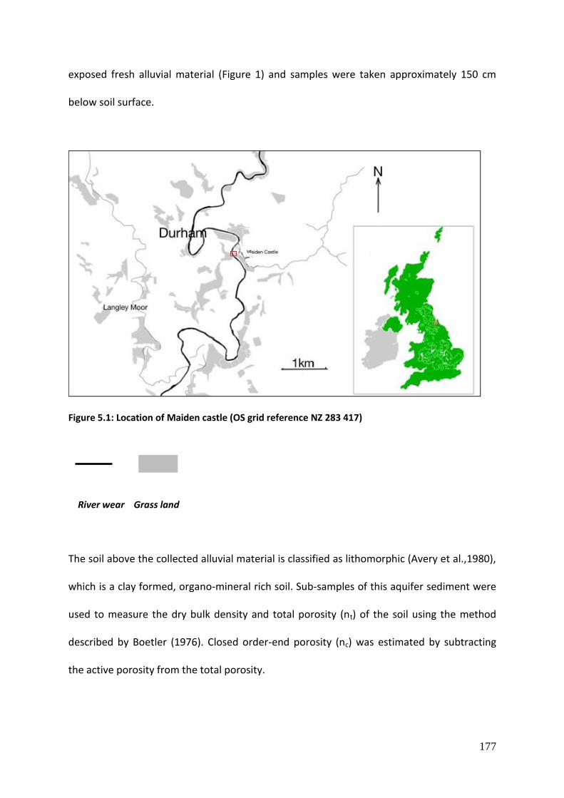
177

exposed fresh alluvial material (Figure 1) and samples were taken approximately 150 cm

below soil surface.

Figure 5.1: Location of Maiden castle (OS grid reference NZ 283 417)

River wear Grass land

The soil above the collected alluvial material is classified as lithomorphic (Avery et al.,1980),

which is a clay formed, organo-mineral rich soil. Sub-samples of this aquifer sediment were

used to measure the dry bulk density and total porosity (nt) of the soil using the method

described by Boetler (1976). Closed order-end porosity (nc) was estimated by subtracting

the active porosity from the total porosity.

178

5.2.3 Batch experiments

Solute retardation may arise from adsorption, biological uptake, chemical factions, and

matrix diffusion (Hoag and Price, 1997). Adsorption of the DOC on soil is a rapid reaction

and the degradation of DOC is a minor factor compared to adsorption in the process of

migration in soil (Li and Shuman, 1997). The retardation assumed the linear adsorption

isotherm in soil; therefore a batch experiment can be used to predict the retardation in the

soil column. The adsorption isotherm for DOC has been found to be linear for soils (Jardine

et al., 1989; Li and Shuman, 1997). Although later studies (Baumgarten et al., 2011) found

the soil adsorption may not be linear, sandy soil adsorption may be more linear than clayey.

To obtain DOC adsorption information from the river bank samples, a series of batch

experiment evaluated at different soil to solution ratios was designed to illustrate DOC

changes. Two approaches were included in these batch experiments. A set of eluent

dilution experiment was designed to access the changes of DOC adsorption for various

solute weights (the river bank samples). The method used in this chapter to get DOC

concentration is sensitive to its upper detection limit (around 65 mg C/l). If the eluent DOC

concentration is over or close to the detection limit of the method used here, dilution of the

eluent would be required to ensure the accurate DOC concentration. Besides the effects to

access the type one error of the DOC methods, the eluent dilution batch experiment was

also designed to use the distilled water (DI water) as the original eluent to access the DOC

released from various soil to solution ratios (river bank samples).

179

5.2.3.1 Eluent dilution experiment

Three sets of 5 polyethylene bottles (120 ml volume) were used in this study, each set of

them were numbered from 1 to 5. The experiments were conducted with varying masses of

river bank sample (60g, 50g, 40g, 30g, 20g respectively), which were mixed with the

standard DOC concentration solutions (32 mg C/l) in the first set of bottles. Therefore, 5 soil

to solution ratios (1:2, 1:2.4, 1:3, 1:4 and 1:6 w/v) were used in the eluent dilution

experiment. The original eluent water were then diluted twice and added to two

polyethylene bottles. Additionally, a pair of batch experiment was conducted using DI water

as eluent. The 25 bottles of suspensions were shaken for 48 h in the dark at 20 oC. The

suspensions were then centrifuged at 3000 min-1 for 15 minutes. Supernatants were then

filtered through 0.45 µm filters. The solutions were then analysed for pH and conductivity.

Eluant DOC concentration was measured using the method of Bartlett and Ross (1998).

Relative DOC concentration changes were calculated as C/Co. where C represents the

solution DOC concentration and Co is the original DOC concentration from the standard

solutions.

Sorption of DOC to the sampled soil was analyzed by use of the initial mass (IM)

relationship (Nodvin et al., 1986). The initial mass method has been a common way to

access DOC sorption in soils (e.g. Kaiser et al., 1996; Kothawala et al., 2008). The IM

approach plotted the concentration of DOC adsorbed or released (Normalised to soil mass,

mg/kg, RE) against the initial DOC concentration of the eluent (Normalised to soil mass,

mg/kg, Xi ). The regression given below:

RE = mXi –b Eq 5.1

The gradient of linear regression (m) is a partition coefficient which measures for the

affinity of the DOC to the eluent. The intercept b is named as desorption term which

180

indicates the amount of DOC released from the soil when the eluent DOC concentration is

zero.

5.2.3.2 Soil wash experiment

Batch experiments of eluate dilution were evaluated at 10 different soil to solution ratios

(1:12, 3:40, 1:15, 7:120, 1:20, 1:24,1:30, 1:40, 1:60 and 1:120 w/v ). The ratios were defined

by the variances of the soil weight applied to the solution range from 10 g to 1 g,

respectively. Soil weight changes were minimized in each individual experiment bottle

between each wash. The batch experiment used DI water as eluent. Suspensions were then

centrifuged at 3000 min-1 for 15 minutes. Supernatants were then separated from the soil.

Same analysis of the eluent dilution was applied on the supernatants. A wash was

performed by adding DI water to each individual bottle to bring it up to its original solution

volume (120 ml). Analysis of DOC was applied on the wash supernatant. The wash of the soil

was repeated three times.

5.2.4 Column Experiment

A 0.60 m long soil core was taken from a Durham river bank. The core was

transported to the laboratory and repacked in the column of the height of 65 cm and

diameter of 15 cm (Figure 2). At the 15 cm tall position of the column, a 15 mm dimension

hole was drilled. A collecting pipe was installed in the middle of the column and linked with

a 1 meter long tube (15 mm diameter). The tube was then linked to a peristaltic pump set

to work at a rate of 0.2×10-3 m/s, there are 34 cm soil packed in between the collecting pipe

181

and the bottom of the elution water. Underneath the collecting pipe, 15 cm sandy soils

were packed up to the bottom of the pipe.

The experimental setup consisted of one unsaturated column of repacked river bank

sediment within a cylinder of inner diameter 150 mm and length 1m - the setup is shown in

Figure 2. The column experiment was conducted at room temperature (approx. 22oC).

Influent water (previously kept at 4oC in the fridge) was brought up to column temperature

before application to the columns by placing a portion of the influent tubing in a warm

water bath.

Figure 5.2: Experimental column set up.

Four small holes were drilled at 1 cm below the top of the column. By doing so, a 15 cm

deep water table was maintained during every refilling of eluting water. The refilling rates

were kept constant during each run, albeit rates varied between runs. Three refilling times

were selected, 75 min, 90 min and 180 min. Three refilling times were then referred to as

182

RF1, RF2 and RF3, respectively, in later analysis. The DOC sorption curve was measured by

plotting DOC changes vs time on each individual run. In this experiment, DOC flux changes

between the extracted solution and elution water were the same as the DOC concentration

changes because the pumping rates were constant during each experiment. Source eluent

water DOC concentration remained constant during all tests (48.13 mg C/l). Following each

run, the column was flushed with distilled water for 3 hours and drained to ensure similar

starting conditions between each run. Similar to the batch experiment, this column study

used both distilled water (DI) water and DOC water as the eluent. DI water was applied to

the column to access the control data while the DOC eluents were used as the experimental

eluent. Experiments started with three days of the distilled water (DI) run through the

column. The average elution time was measured as the time from the introduction of the

sample at the top of the column to the first appearance of DOC in the collected waters. DI

water was used to perform three blank runs with refilling time of 75 mins, 90 mins and 180

min which were named as event RF1, RF2 and RF3. In the first three days of the RF1

experiment, elution water was added by different time gaps. 200 ml eluent was adding in

the system to top up the column. The first day of RF1 experiment the run was for 120 mins.

No additional elution water was added to the system except at beginning of the first day of

the RF1 experiment. The elution water extracted from three blank runs were collected as

the control data. Following the three blank runs, DOC eluent water was applied to the

column system. The collected samples were immediately filtered upon collection through a

0.45 µm filter and then pH, conductivity and DOC concentration were measured. In the

experiment, the eluate DOC concentration over eluent DOC concentration was used to

indicate the concentration changes over each individual run. In addition to DOC changes,

experimental eluate DOC concentration relative to control eluate DOC concentration

183

(Relative DOC) under three different refilling times was used as indication of changes in the

river bank sample adsorption/desorption.

5.3. Results and discussion

5.3.1 Results of the batch experiments

5.3.1.1 Results of eluent dilution experiment

The bulk density of the infilling river bank samples used in experiment was 1.23 g/cm3.

The C/Co increased with the decreasing elusion water DOC concentrations in the batch

experiment. The DOC concentration changes between different soil weights are small in the

lower elution water concentrations with an average 6.43% DOC concentration changes after

the first dilution and 6.98% after the second dilution. DOC concentration changes between

different soil weights were bigger in the original elusion water, which merely reached 8.52%

concentration changes (Table 5.1). Overall, the batch experiment with elution water didn’t

find significant DOC concentration changes between soil weights in the range used. Results

of batch experiment on DOC solute transport also didn’t show any clear link between the

different pore volumes used (Table 5.2).

DOC original Average C/CO Changes between

different soil weights

Original 33.23 1.66 8.52%

1st Dilution 16.62 3.63 6.43%

2nd Dilution 8.31 7.54 6.98%

Table 5.1: DOC changes over original DOC eluent concentration after two dilutions.

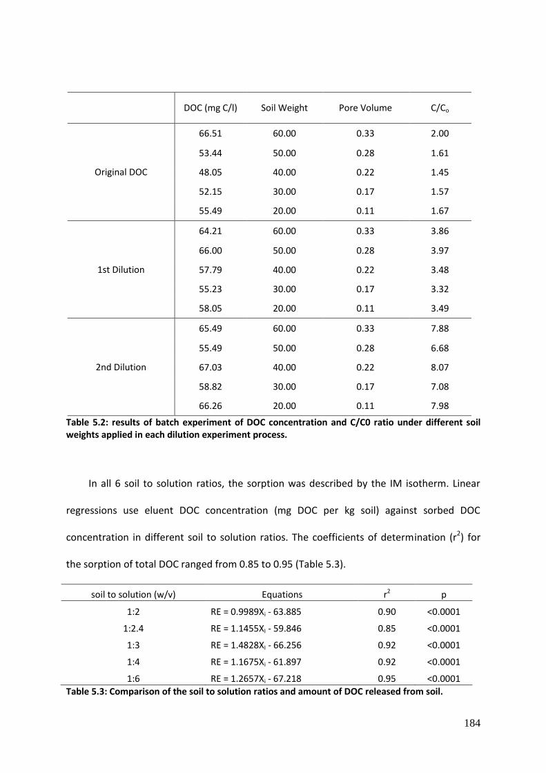
184

DOC (mg C/l) Soil Weight Pore Volume C/Co

Original DOC

66.51 60.00 0.33 2.00

53.44 50.00 0.28 1.61

48.05 40.00 0.22 1.45

52.15 30.00 0.17 1.57

55.49 20.00 0.11 1.67

1st Dilution

64.21 60.00 0.33 3.86

66.00 50.00 0.28 3.97

57.79 40.00 0.22 3.48

55.23 30.00 0.17 3.32

58.05 20.00 0.11 3.49

2nd Dilution

65.49 60.00 0.33 7.88

55.49 50.00 0.28 6.68

67.03 40.00 0.22 8.07

58.82 30.00 0.17 7.08

66.26 20.00 0.11 7.98

Table 5.2: results of batch experiment of DOC concentration and C/C0 ratio under different soil weights applied in each dilution experiment process.

In all 6 soil to solution ratios, the sorption was described by the IM isotherm. Linear

regressions use eluent DOC concentration (mg DOC per kg soil) against sorbed DOC

concentration in different soil to solution ratios. The coefficients of determination (r2) for

the sorption of total DOC ranged from 0.85 to 0.95 (Table 5.3).

soil to solution (w/v) Equations r2 p

1:2 RE = 0.9989Xi - 63.885 0.90 <0.0001

1:2.4 RE = 1.1455XI - 59.846 0.85 <0.0001

1:3 RE = 1.4828XI - 66.256 0.92 <0.0001

1:4 RE = 1.1675Xi - 61.897 0.92 <0.0001

1:6 RE = 1.2657Xi - 67.218 0.95 <0.0001

Table 5.3: Comparison of the soil to solution ratios and amount of DOC released from soil.

185

In Table 5.3, parameter b (intercepts of equation) represents the DOC released from the soil

when the eluent DOC concentration is 0 mg/kg. Comparing the different soil to solution ratio on the

parameter b, the ratios differences influence on b was found to be minor. A regression including all

soil to solution ratios were listed below:

RE =1.21 Xi - 63.8 Eq 5.2

The r2 of equation 1.2 is 0.85 and P value is smaller than 0.001. The parameter m

(1.21), was dependent from the changes of ratios. The IM isotherm indicates an average of

the 63.8 mg/kg DOC will be released from sample soil in experiments.

210

40.00%

20.00%

0.00%

-20.00%

-40.00%

-60.00%

Dilution

Re

lati

ve

DO

C c

ha

ng

es

Figure 5.3: Boxplot of the relative DOC changes over 2 dilutions in eluent dilution experiment.

186

. Results (Figure 5.3) showed relative DOC concentration changes were decreased over

all three eluent DOC concentrations. The original eluent DOC concentration batch had a

median relative DOC concentration of -9.8%. First dilution and second dilution had the

relative median DOC changes of -0.5% and -16.5%, respectively. The negative relative DOC

changes indicated the adsorption of the river bank samples after the batch experiment. In

Figure 5.3, the relative DOC changes weren’t increased or decreased with dilution of the

eluent, although both Table 1 and 2 indicated that the DOC changes were increased in all

batch samples. The adsorption may therefore need longer travel distance to build up the

better removed rate and eventually suppress the eluent DOC concentration. Figure 5.4

showed relative DOC changes over different samples weights. In all 5 median values of the

relative DOC changes over soil to solution ratio, only the 1:4 ratio (30 g soil) has a positive

reading of 1.2%. The rest of the sample weight had the relative DOC changes of -13.4% (1:6),

-5.3% (1:3), -0.5% (1:2.4), -11.5% (1:2). The positive reading of relative DOC concentration

indicated net desorption of DOC and the negative reading indicated the adsorption of the

samples. Majority of the samples in this eluent dilution experiment showed adsorption of

DOC. However, the relationship between soil to solution ratio and relative DOC change was

not linear. Exceptions of the soil to solution ratios and relative DOC changes may be due to

the turbulence of the shaking table overnight i.e. clogging may formed prior to the shaking

on some samples therefore limited the sample interaction with the eluent.

187

1:21:2.41:31:41:6

40.00%

20.00%

0.00%

-20.00%

-40.00%

-60.00%

Soil to solution ratio

Re

lati

ve

DO

C c

ha

ng

es

Figure 5.4: Relative DOC changes over different soil to solution ratios.

Comparison of the IM isotherm and relative DOC concentration over dilutions found

that soil adsorption of DOC were the dominated Figure of sample soil sorption albeit the

much smaller initial eluent DOC (33.2 mg/kg) input compare potential DOC desorption b

(63.8 mg/kg).

5.3.1.2 Results of soil wash experiments

The solute was then changed from stream water to the DI water. In total 10 different soil

to solution ratios were chosen to evaluate the DOC sorption to soil. Despite different soil to

solution ratios applied in eluate dilution process, DOC concentration maintains on average

of 60 mg C/l. In total 20 samples in 2 batches, DOC concentration varied from 52 mg C/l to

188

62 mg C/l.. After 3 washes, solutions concentrations from 60 samples in 6 batches still

showed an average DOC concentration of 59 mg C/l ranging from 48 mg C/l to 63 mg C/l.

Results of batch experiments showed large export of DOC in both elusion water and DI

water. Desorption from the soil may be the source of the continually high DOC

concentration in the solution. In between each wash of distilled water conductivities were

significantly decreased from 91 to 2

changes of pH and conductivities may be caused by the changes of DOC concentration.

210

7.3

7.2

7.1

7.0

6.9

6.8

6.7

Dilution

pH

210

900

800

700

600

500

400

300

Dilution

Co

nd

uctiv

ity

210

65

60

55

50

Dilution

DO

C (

PP

M)

Figure 5.5: DOC concentration changes / solution hydrological changes over eluent dilute process.

3210

7.0

6.5

6.0

5.5

5.0

wash

pH

3210

100

80

60

40

20

0

wash

Co

nd

uctiv

ity

3210

70

65

60

55

50

wash

DO

C (

PP

M)

Figure 5.6: DOC concentration changes / solution hydrological changes over wash process. Where 3 graphs stand for pH, conductivity and DOC changes between each dilution and wash process, respectively.

Figure 5.5 shows the comparison between eluent dilution processes that were applied in

the soil batch experiments. Results of these dilutions process showed that both pH and

conductivity of the solution decreased with increased number of dilution steps. The DOC

concentration from the solution increased with the deceased eluent DOC concentration.

The volume of eluent water added to each experimental bottle was the same for the

189

previous dilution process in section 5.3.1.1. As the eluent DOC decreased over each dilution,

the increased solution DOC must be sourced from desorption from the soil.

In comparison to the dilution experiment, the soil batch experiment was also designed

to use DI water to perform a set of wash experiments. Wash experiments showed a rapid

increase of pH between the original solution and the first wash (9.6%). From first to third

washes, solution pH decreased. The conductivities decreased with increased washing times.

Median of DOC concentrations remained the same between each wash. Similar to the

earlier dilution process, the volume of DI water added to each bottle remained the same

between each wash (Figure 5.6). Although the b from IM isotherm varies with the different

soil to solution ratios, the DOC concentration between each wash in Figure 5.6 appeared to

be relatively stable. The stable DOC concentrations after each wash indicated equilibrium

may have existed during the experiment.

5.3.2 Results of the column study

5.3.2.1 DI eluent experiment

The first set of column studies on the DOC concentration changes during the first three

days of experiment were performed using distilled water as the eluting solution (Figure 5.7).

Although all three experiments were conducted using different experimental duration, only

the first day of experiment showed a potential breakthrough curve over the 60 minutes of

the experiment. The oscillation of DOC concentration between 10 mg c/l to 50 mg c/l is

observed between RF2 and RF3.

190

During the RF1 (75 min) experiment (Figure 5.7), DOC concentration changed from 38.8

mg C/l to 57.9 mg C/l in first 15 min of the experiment. DOC concentration then slowly

decreased from 57.9 mg C/l to 48.3 mg C/l during the next 45 mins before a small increase

on the end of first day experiment (49 mg C/l). Unlike the smooth transition of the DOC

concentration changes in the first day, the two experiment lengths RF2 and RF3 illustrated

DOC concentration from extracted solutions from column had rather constant changes in

times of 15min or 30 min.

Figure 5.8 shows the whisker plot of DOC concentration changes over three running

times. Three median values were observed 52.32 mg C/l for RF1, 26.97 mg C/l for RF2 mins

and 35.12 mg C/l for RF3. With the extension of the running time, DOC concentrations

decreased, except RF3 where the median value here were slightly increased to 35.12 mg C/l

compared to 26.97 mg C/l in the 90 mins run.

In general, ranges of DOC concentration for the last two days of the experiments

fluctuated on average by 40 mg C/l compared to changes on the first day experiment where

DOC concentrations only changed on average by 15 mg C/l (Figure 5.7). The rapid changes

of DOC concentration in solution showed the release of DOC from soil is a rapid desorption -

there was about 30 mins in between the concentration peaks.

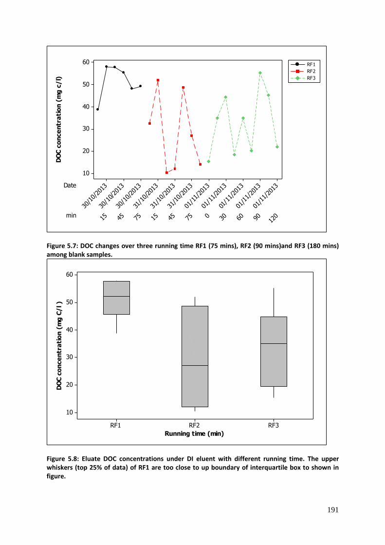
191

min

Date

1209060300754515754515

01/11/

2013

01/11/

2013

01/1

1/20

13

01/1

1/20

13

01/11/

2013

31/10/

2013

31/10/

2013

31/1

0/20

13

30/1

0/20

13

30/1

0/20

13

30/10/

2013

60

50

40

30

20

10

DO

C c

on

ce

ntr

ati

on

(m

g c

/l)

RF1

RF2

RF3

Figure 5.7: DOC changes over three running time RF1 (75 mins), RF2 (90 mins)and RF3 (180 mins) among blank samples.

RF3RF2RF1

60

50

40

30

20

10

Running time (min)

DO

C c

on

ce

ntr

ati

on

(m

g C

/l )

Figure 5.8: Eluate DOC concentrations under DI eluent with different running time. The upper whiskers (top 25% of data) of RF1 are too close to up boundary of interquartile box to shown in figure.

192

5.3.2.2 DOC eluent experiment

5.3.2.2.1. 75 mins (RF1) experiment

The results of soil column studies were then conducted using a 48.13 mg C/l

concentration DOC eluent. From 04/11/2013 to 06 /11 /2013, DOC concentration changes

were monitored in comparison with the original DOC concentration of eluent used in the

experiment. Results of the first day experiment showed a rapid decrease of DOC

concentration and flux changes (Figure 5.9). The flush of elution water brought about the

positive increase in DOC compared to the original DOC concentration changes in the first 30

mins; DOC concentration reached the lowest point after 75 mins. Immediate after 75 mins,

DOC concentration returned back to a relative high DOC concentration in the next 15 mins.

Similar changes of DOC concentration were observed in the next two days of the

experiment. Differences of the experimental design of the time between each eluent top up

may cause the different lag time of the appearance of DOC concentration peaks in each day.

Figure 5.10 shows the eluate DOC changes from DOC eluent relative to eluate DOC from

DI eluent for the RF1 experiment. Relative DOC concentration has the median values of –

63.7% among non- refilling samples and median values of -67.9% in refilling points. The

negative value of the relative DOC changes indicates the adsorption of river bank samples

were the main driver of the DOC changes through the RF1 experiment.

193

1201059075604530150

0.00%

-10.00%

-20.00%

-30.00%

-40.00%

-50.00%

-60.00%

-70.00%

-80.00%

-90.00%

min

DO

C c

on

ce

ntr

ati

on

ch

an

ge

s

120

105

90

75

6045

30

150

Figure 5.9: time series of DOC changes on every RF1 experiment.

YN

0.00%

-10.00%

-20.00%

-30.00%

-40.00%

-50.00%

-60.00%

-70.00%

-80.00%

-90.00%

Sample Input

Re

lati

ve

DO

C

Figure 5.10: Relative DOC over RF1 experiment. There was only 1 time sample input, therefore the plot box of Y is represented as a single line.

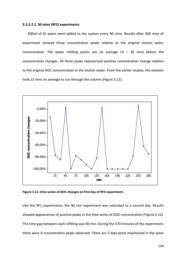
194

5.3.2.2.2. 90 mins (RF2) experiments

200ml of DI water were added to the system every 90 mins. Results after 300 mins of

experiment showed three concentration peaks relative to the original elution water

concentration. The water refilling points are on average 15 – 30 mins before the

concentration changes. All three peaks represented positive concentration change relative

to the original DOC concentration in the elution water. From the earlier studies, the solution

took 22 mins on average to run through the column (Figure 5.11).

285255225195165135105754515

0.00%

-20.00%

-40.00%

-60.00%

-80.00%

-100.00%

min

DO

C c

on

ce

ntr

ati

on

ch

an

ge

s

Figure 5.11: time series of DOC changes on first day of RF2 experiment.

Like the RF1 experiments, the 90 min experiment was extended to a second day. Results

showed appearances of positive peaks in the time series of DOC concentration (Figure 5.12).

The time gap between each refilling was 90 min. During the 570 minutes of the experiment,

there were 6 concentration peaks observed. There are 5 data point maintained in the same

195

concentration changes after the second peak. The absorbance of 5 samples is over the limit

(60 mg C/l) of the top measurement which means their actual DOC concentrations were too

small to measure.

During the 2 days of the experiment, DOC concentrations decreased by 75% compared to

the DOC concentration in the elution water. The peak concentrations increased 3.4%

compared to the original DOC concentration. The DOC concentrations increases may be due

to soil to solution equilibrium illustrated by batch experiment changes.

52546540534528522516510545

20.00%

0.00%

-20.00%

-40.00%

-60.00%

-80.00%

-100.00%

min

DO

C c

on

ce

ntr

ati

on

ch

an

ge

s

Figure 5.12: time series of DOC changes on second day of RF2 experiment.

196

YN

100.00%

50.00%

0.00%

-50.00%

-100.00%

Sample Input

Re

lati

ve

DO

C

Figure 5.13: Relative DOC changes during RF2 experiment.

Figure 5.13 shows that relative DOC changes over the 2 days of 90 mins experiment. The

median relative DOC changes on both refilling samples and non-refilling samples were -

61.2% and 61.6%, respectively. Similar to the earlier 75 mins experiment, adsorption of the

river bank samples were the dominant factor during the experiment. The peak in the DOC

changes per se is the therefore merely the reflection of the refilling.

5.3.2.2.3. 180 mins (RF3) experiments

The time gap between each refilling was extended to 180 mins on the RF3 experiments.

The results RF3 experiments showed the time gap between two peak concentrations

extended to 90 mins and DOC concentration increased to a maximum of 35% greater than

the original elution water concentration. The RF3 experiment was conducted three days

after the previous RF2 experiment. During the three day experiment gap, the water table

went down about 2 cm. No additional water was added during the time between the two

197

experiments. The first day of the RF3 experiment had two concentration peaks (Figure 5.14);

both of them appeared 30 mins after the refilling of the sample water. Two DOC

concentration peaks represented increases in DOC concentration relative to the eluent DOC

concentration. The majority of samples collected reflect decreases in the DOC

concentrations after water has run through the column. Figure 5.15 shows median value of

the relative DOC changes in no-refilling samples of -58.5%. Median values of refilling

samples increased 1% compared to the no refilling samples.

3903453002552101651207530

50.00%

25.00%

0.00%

-25.00%

-50.00%

-75.00%

-100.00%

min

DO

C c

ha

ng

es

Figure 5.14: time series of DOC changes on every 180 mins refiling

198

YN

-40.00%

-50.00%

-60.00%

-70.00%

-80.00%

-90.00%

Sample Input

Re

lati

ve

DO

C

Figure 5.15: Relative DOC changes during 180 mins experiment. During the experiment, there were only two times sample inputs, therefore the upper and lower boundaries of Y were same as interquartile box.

When the experimental time was extended to 720 min, similar DOC concentration trends

to the RF2 experiment were observed (Figure 5.16). The time between each refilling was on

average 90 mins. The exception was between the third and fourth refilling, which has a time

gap between each refilling of 180 min. The peak of the concentration peaks appeared 15 to

30 min after each refilling. The majority of the DOC concentrations showed a reduction

compared to the original elution water concentration. Between peak 3 and peak 5, refilling

time were increased to the 180 min, the DOC peak shifted with the increased time between

elution.

During the experiment, DOC peaks were observed between 15 mins to 30 mins after

refiling eluent to the system and stayed relatively stable compared to the negative changes

observed from DOC concentration. It is most likely the DOC peak was brought up by the

199

refilling of the elution water. During 720 min, the delay of the DOC concentration peak

increased with the extension of the time between each refilling. Average peak DOC

concentration increased from 3.4% to 20% as the extension of refilling time increased. All

three experiments (RF1 , RF2 and RF3) observed an increase of pH over the experimental

time, albeit conductivity of infiltration samples showed no clear relationship within the

experimental time series. The relatively stable DOC peaks seem strongly associated with

refilling of the water, which indicates these peaks were the delayed appearance of refilling

the elution water.

During all three experiments, the eluent water was maintained at the same DOC

concentration. The majority of the DOC was removed through running through the column,

with average reduction in DOC concentration being 74%. Even with the extended time

between each refilling, the removal of DOC still didn’t achieve any form of breakthrough

curve or equilibrium of DOC removal. Relative DOC changes in between three experiments

(Figure 5.17) were slightly increased with the increasing refilling time gap. The extension of

the refilling gap leads to longer running time, therefore the longer running time seemed to

decrease the adsorption (increased desorption) by the river bank sediment. The batch

experiment indicates soil sorption is independent to the different soil to solution ratios.

Therefore, the greater soil content and the greater soil: water ratio of the column

experiments relative to the batch experiments may not have an impact on the soil

adsorption equilibrium, but the longer running time of the eluent should enhance the

sample removal process.

200

660585510435360285210135600

40.00%

20.00%

0.00%

-20.00%

-40.00%

-60.00%

-80.00%

-100.00%

min

DO

C c

ha

ng

es

Figure 5.16: time series of DOC changes on extended time

Batch experiments indicated an equilibrium of DOC with the soil. However, the column

studies showed adsorption of influent DOC. After two days of blank runs, the system may

have converted to anaerobic which would lead to enhanced DOC removal. During the entire

column experiment, no clear pH and conductivity changes were observed. The DOC changes

are mainly controlled by the soil sorption. The peaks observed in the column study

commonly appeared after refilling of the eluent DOC. The observed peaks may be caused by

various reasons. One simple explanation is that the eluent DOC passes through micropores

present in the soil column. Studies conducted on DOC export in other soil systems, i.e.

grassland and agricultural soils, indicate that DOC transport are primarily determined by

hydrological regime, especially in the vertical direction (Mertens et al., 2007; De Troyer et

al., 2011). Peaks during column experiments may indicate that vertical flux also as a main

control of the bank filtration impact. However, the pumping rate used in the column

201

experiment were relatively low compared to the industrial bank filtration, therefore,

different pumping rate may overtake the vertical water flux to control the DOC transport

through soil. Kaiser and Zech (1997) indicted a relationship between reduced DOC sorption

at the greater DOC addition. Here in the column study, the additional DOC by refilling may

just indicate the rebalance of the soil solution equilibrium since especially that eluent DOC

concentration are much smaller than the potential desorption DOC concentration of

sampled soil.

RF3RF2RF1

0.00%

-20.00%

-40.00%

-60.00%

-80.00%

-100.00%

Re

lati

ve

DO

C

Figure 5.17: Relative DOC changes over three experiments

202

5.4 Conclusions

In the batch experiment, the isotherm result indicated an average of 63.8 mg C g/l

desorption would occur in the soil sample applied in this study. With the elution DOC

concentration varying from 8 mg C g/l to 32 mg C g/l which are much less than the initial

DOC concentration desorbed from soil. The soil batch experiment still shows the strong

feature of DOC absorption. DOC was successfully removed by running through a soil column

with the average removal rate of 74% relative to initial concentration. Numerous stable DOC

peaks were spotted 15 to 30 mins after each refilling of elusion water suggesting the column

may be mainly control by absorption, rather than desorption of the soil. The fluctuations in

DOC concentration observed between peaks may be caused by biomass activities or

absorption/ desorption equilibrium. No breakthrough curve of DOC concentration was

observed in this study.

203

Chapter 6 Conclusion 6.1 Progress against study objectives

Objective 1

Measurement of the DOC concentration and budget on a series of nested and blocked

catchments.

Drainage is a commonly used upland peat management technique in the UK and has driven

the interests of researchers as drainage has been associated with increased water colour

and changes in carbon storage in peat land. Blocking has been suggested as an alternative

to peat land restoration to reduce the water colour and prevent carbon loss. The study,

based on four years observation from 2008 to 2012 in Upper Teesdale, Northern England,

has shown that both DOC concentration and DOC export did decrease upon drain blocking.

For DOC concentration, the effect of drain-blocking was to lower concentration - at larger

catchment scales (1 km 2) a 4% reduction was found and a 2.9% reduction for zero order

drains. For the DOC export, there was a 7% reduction on first order drains ( 1 km2) and 12%

reduction on zero order drains. However, it was shown that any observed decrease in DOC

export was largely explained by changes in water yield rather than the drain blocking itself.

It is possible that the small change in concentration observed at this site is due to the

relative small change in water table that was brought about by the drain blocking at this

site.

204

Objective 2

To access the blocking effects upon the peak flow events in upland peat.

A series of analyses were applied to the DOC data gathered from 2008 to 2012. From 4

years of observations a total of 756 peak flow events could be considered. Results of events

analysis found that both the change in DOC concentration and the change in DOC flux across

an event was smaller after blocking with an average of 4 times smaller in DOC concentration

changes after blocking and 55.6 % reduction on DOC flux changes after blocking. Blocking is

a significant factor controlling the DOC concentration and DOC flux changes by controlling

the event flow in the events analysis. Despite the blocking effects on controlling the event

flow, factors such as rainfall total, rain duration, flow lag time, peak flow were also observed

as significant factors controlling the event flow. Principal components analysis of the events

data indicated interactions between rainfall duration and flow lag time were the more

dominant factors controlling the event flow thus the DOC changes of the events.

In general, the effects of drain blocking on DOC concentration changes and DOC flux

changes increased with scale of drains after blocking.

Objective 3

To assess bank filtration as an alternative approach to the management of high DOC

concentrations.

Bank filtration is primarily used in Germany as an efficient water treatment for bulk

contaminants and water colour. The study was aimed to test whether bank filtration could

205

serve as an efficient treatment for DOC removal as an alternative to drain blocking. Instead

of conducting a field study, a series of batch experiments and a column study were

conducted in the laboratory for 6 months. Soil samples were gathered on the river bank of

River Wear, Durham. Results of batch experiments were applied on different soil to solution

ratios and showed an average of 63.8 mg/kg DOC will be released from the soil. Despite the

initial desorption of DOC from soil been higher than any input eluent DOC concentration

applied in the batch experiments, the eluate DOC concentration relative to eluent DOC

concentration still showed reduction of relative DOC concentration varying from 0.5% to

16.5%. The batch experiment indicated soil sorption is the key factor controlling the DOC

connection changes.

In the column study, the results of relative DOC eluate concentration showed an

average of 74% reduction. The DOC concentrations of soil water after the filtration were

generally higher than the DOC concentration input. Soil sorption equilibrium was attained

between the eluent DOC concentration and soil. The desorption/adsorption status of the

soil was shown to responds to the infilling of the DOC eluent. Although the eluate DOC level

were higher than the eluent DOC in the column study, the eluate DOC shows the reduction

in comparison between the DOC eluent and distilled water eluent. The study indicates that

bank filtration could be a useful technique to reduce stream DOC concentration if the

stream contains high DOC concentrations. With the soil sample used in this study, an eluent

DOC concentration more than 63.5 mg C/l may start to show real reduction in the eluate

through filtration. However, the stream DOC concentrations applied in the study were much

less than the initial soil desorption DOC concentration observed. Thus, the bank filtration

may not be suitable for the studied site. In most of UK highland peat, the stream DOC

concentration is also much less than 63.5 mg C/l. Therefore, river bank filtration may an

206

efficient way in controlling the DOC if at an industrial level for heavily polluted water pre-

treatment, but seemed not suitable for the normal reservation of DOC management.

Objective 4

to assess the impact of revegetation on DOC changes in upland peat streams.

A year long field study of revegetation effects on DOC concentration and water colour

in streams was conducted at Killhope, Northern England. The revegetation effects on DOC

concentration and water colour was assessed as relative DOC and relative water colour. In

the study, no water sample or the metrological data were taken prior to the start of

experiment, therefore, the relative data was not used to assess whether the DOC

concentrations or water colour are different between the study catchments but whether

the DOC and water colour in the stream runoff in the experimental catchment declines

relative to the control catchment with time.

Results of DOC concentration showed the higher DOC concentration in experimental

catchments than control catchment with the average of 41.68 mg C/l DOC in experimental

catchment and 31.65 mg C/l DOC in the control catchment during the study period. A

significant difference in DOC concentration between the sample types was observed. i.e. the

difference between catchments is 12.1% higher in runoff samples than in stream water

samples. The results for the relative DOC concentration showed no significant trend of

relative DOC concentration over the study months. During the study periods, the

revegetation was found not to be a significant factor in controlling DOC concentration.

Results of water colour shared some similarities with results for DOC concentration. The

experimental catchment had the higher water colour and more humic compounds than the

207

control catchment. The difference of both absorbance at 400 nm absorbance and the E4/E6

ratios are higher in runoff samples in between catchments than in stream water samples.

Unlike the relative DOC concentration, the relative water colour observed a seasonal change

over the study months. The variation of both relative absorbance at 400 nm absorbance and

E4/E6 ratio in between months got smaller from spring to winter. A reverse trend in

between relative absorbance at 400 nm absorbance and E4/E6 ratio was also observed

which indicates higher water colour but less humic compound were produced between

these seasons. Thus, a potential flow path changes may have occurred during the study. In

general, the revegetation was found not to be a significant factor controlling the water

colour changes. However, the effect of revegetation is much influenced by factors such as

rainfall and seasonal changes.

Despite lack of encouraging results of DOC concentration and water colour observed,

the effects of revegetation were observed as efficient for maintaining on average 0.16 m

higher water table in the experimental catchment than the control catchment and lower

variances in evaporation in between months in the experimental catchment (39.2% changes

in evaporation between months).

6.2 Study limitations

Limitations inherent in the methods and data used in this study are acknowledged during

the study. In the drain blocking and events analysis, the large number of samples collected

in the drain sampling campaigns make it impossible to directly analyse DOC concentration

on each sample, and therefore absorbance was used as a proxy for DOC. Regular calibration

experiments for this relationship were carried out which indicated that the adoption of

individual calibration curves for each sites was appropriate for these data.

208

The data collected was also limited by the nature of the environment in which both drain

blocking and revegetation were conducted. In drain blocking study, six monitoring sites

were equipped with a range of scientific instrumentation including automatic water

samplers and data loggers set up to monitor flow, conductivity and a range of weather

parameters. The extreme weather conditions at the localities leads to the breakdown of

equipment at certain times and thus leads to the loss of data. The panels used in

revegetation suffered the same severe weather conditions with 1 m deep snow in the

bottom of both catchments where the automatic water samplers (along with wiring in the

data loggers) got buried from December 2013 to February 2014. The summer of 2013 also

had some cruel effects on the sampling at revegetation site, for the 3 months from June to

August, both the control and the experimental catchments suffered from extreme dry

conditions meaning auto samplers failed (Figure 6.1). Measures were taken to reduce the

impact of damage, for example, additional solar panels were installed on both catchments

to provide enough power for auto samplers during the winter snow periods. Both auto-

samplers were also moved to the higher position to avoid entirely being buried by snow. In

the dry summer, the spot samples were taken in addition to the auto samples and traced all

the way down to the main stream in both catchments.

209

Figure 6.1: Picture of Killhope, County Durham. a) Taken in February 2013 of experimental catchment. b) Taken in June 2013 of experimental catchment.

The field management is also leads to some data gaps. As both drain blocking site and

revegetation site were primarily used for grouse shooting, the visit to the site was limited

during the shooting season: on average one and half months twice a year at both sites. At

the revegetation site, the meteorological tower in the control catchment is located in the

distance sight of a shooting butt. and therefore was taken down by the gamekeeper. The

lack of the control meteorological data makes the comparisons between the evaporation

and the energy budget between the catchments impossible and thus the data comparison is

mainly based on the water tables in between catchments.

a b

210

6.2 Overall Conclusion

This thesis is primarily focused on the impacts of a series of peat land management

strategies (drain blocking and revegetation) on DOC changes. Both drain blocking and

revegetation showed limited impacts on the DOC, with ranges of 2.2% – 4% change of DOC

concentration observed upon drain blocking and no clear changes of DOC upon

revegetation. The impacts of drain blocking on revegetation were noticed when a stable

water table was achieved by drain blocking (Worrall et al., 2007). Therefore, if drain blocking

and revegetation were conducted in the same study site, a joint impact of two

managements could be expected.

Both drain blocking and revegetation studies indicate significant relations of site and scale

difference. In other words, the same practices of both managements would have different

results when applied to different sites.

Although some of the studies were conducted over 4 years periods (drain blocking), land

managements of drain blocking and revegetation observed small effects over the DOC

concentrations. The land management effects as such were strongly linked to changes of

water table. Studies of water table changes (caused by drought or flood) observed long

lasting effects even 5 years after events (Worrall et al., 2006). Therefore, longer observation

periods may lead to better effects of blocking or revegetation, especially if combined studies

of drain blocking and revegetation were applied, a 5-year study period would be expected.

The bank filtration study was conducted as a side project to test whether it is applicable

to the UK. Results of the column study indicate bank filtration was not suitable as a water

treatment if primarily focused on DOC removal in the UK as the DOC levels were at least 40

mg C g/l lower than the applied soil DOC equilibrium range of bank filtration in the UK.

211

6.3 Future work

Besides the data limitations described during the study, there is some further work that

could be done. Column study was performed on a single column system which is flushed by

deionized water in between different sets of DOC eluent. However, this may lead to

inaccuracy of the comparison between control and experimental data. Therefore, an

additional set of control column could be included in the study.

As various studies indicate that drain blocking would benefit the revegetation in

peatland (Holden et al., 2013). A combined study of drain blocking and revegetation could

be conducted to assess the effects on DOC removal and water colour changes. Also, the

revegetation of land leads to the different buffer time observed during the peak flow event

compared to bare peat, therefore a peak events analysis should be conducted to access the

potential benefit of revegetation effects on DOC removal during the peak flow events. In

terms of limitations of the revegetation study, a series of soil water dipwells were installed

on the experimental catchment during May 2014 in order to trap the soil water under the

extreme dry conditions of the site during the summer. However, the study periods weren't

long enough for the soil water dipwell to trap enough samples, therefore a longer study

periods should be carried out that could take into consideration data from these soil water

traps. In case of the meteorological tower that was taken down in the control catchment,

Brown et al. (2015) indicates using soil thermal regime as a tool to access the vegetation

management. Therefore, an alternative soil regime comparison could be included in

between catchments in the revegetation site to the comparison of energy budget between

catchment.

212

Reference

Anderson, D. W., Saggar, S., Bettany, J. R., & Stewart, J. W. B. (1981). Particle size fractions

and their use in studies of soil organic matter: I. The nature and distribution of forms

of carbon, nitrogen, and sulfur. Soil Science Society of America Journal, 45(4), 767-

772.

Andersson, S., Nilsson, I., & Valeur, I. (1999). Influence of dolomitic lime on DOC and DON

leaching in a forest soil. Biogeochemistry, 47(3), 297-317.

Armstrong, A., Holden, J., Kay, P., Foulger, M., Gledhill, S., McDonald, A. T., & Walker, A.

(2009). Drain-blocking techniques on blanket peat: A framework for best practice.

Journal of Environmental Management, 90(11), 3512-3519.

Armstrong, A., Holden, J., Luxton, K., & Quinton, J. N. (2012). Multi-scale relationship

between peatland vegetation type and dissolved organic carbon concentration.

Ecological Engineering, 47, 182-188.

Austnes, K., Evans, C. D., Eliot-Laize, C., Naden, P. S., & Old, G. H. (2009). Effects of storm

events on mobilisation and in-stream processing of dissolved organic matter (DOM)

in a Welsh peatland catchment. Biogeochemistry, 99(1-3), 157-173.

Avery, B.W., (1980). Soil Classification for England and Wales. (Higher categories). Soil

Survey Technical Monograph No 14.

Baker, A., Tipping, E., Thacker, S. A., & Gondar, D. (2008). Relating dissolved organic matter

fluorescence and functional properties. Chemosphere, 73(11), 1765-1772.

Ballard, C. E., McIntyre, N., Wheater, H. S., Holden, J., & Wallage, Z. E. (2011). Hydrological

modelling of drained blanket peatland. Journal of Hydrology, 407(1), 81-93.

213

Bartlett, R. J., & Ross, D. S. (1988). Colorimetric determination of oxidizable carbon in acid

soil solutions. Soil Science Society of America Journal, 52(4), 1191-1192.

Baumgarten, B., Jaehrig, J., Reemtsma, T., & Jekel, M. (2011). Long term laboratory column

experiments to simulate bank filtration: factors controlling removal of

sulfamethoxazole. Water Research, 45(1), 211-220.

Bellamy, P. E., Stephen, L., Maclean, I. S., & Grant, M. C. (2012). Response of blanket bog

vegetation to drain‐blocking. Applied Vegetation Science, 15(1), 129-135.

Bertilsson, S., & Tranvik, L. J. (2000). Photochemical transformation of dissolved organic

matter in lakes. Limnology and Oceanography, 45(4), 753-762.

Boelter, D.H.(1976). Methods for analysing the hydrological characteristics of organic soils in

marsh-ridden areas. In: Hydrology of Marsh-Ridden Areas. Proceedings of IASH

Symposium Minsk., 1972. IASH, UNESCO, Paris, pp. 161–169.

Boyer, E. W., Hornberger, G. M., Bencala, K. E., & McKnight, D. M. (1997). Response

characteristics of DOC flushing in an alpine catchment. Hydrological Processes,

11(12), 1635-1647.

Brown, L. E., Palmer, S. M., Johnston, K., & Holden, J. (2015). Vegetation management with

fire modifies peatland soil thermal regime. Journal of Environmental Management,

154, 166-176.

Brown, V. A., McDonnell, J. J., Burns, D. A., & Kendall, C. (1999). The role of event water, a

rapid shallow flow component, and catchment size in summer stormflow. Journal of

Hydrology, 217(3), 171-190.

Cannell, M. G. R., Dewar, R. C., & Pyatt, D. G. (1993). Conifer plantations on drained

peatlands in Britain: a net gain or loss of carbon?. Forestry, 66(4), 353-369.

214

Cha, W., Choi, H., Kim, J., & Cho, J. (2005). Water quality dependence on the depth of the

vadose zone in SAT-simulated soil columns. Water Science & Technology: Water

Supply, 5(1), 17-24.

Chatfield, C., & Collins, A. J. (1980) Introduction to multivariate analysis. Chapman and Hall,

London

Chapman, P. J., Clark, J. M., Reynolds, B., & Adamson, J. K. (2008). The influence of organic

acids in relation to acid deposition in controlling the acidity of soil and stream waters

on a seasonal basis. Environmental Pollution, 151(1), 110-120.

Christophersen, N., & Hooper, R. P. (1992). Multivariate analysis of stream water chemical

data: The use of principal components analysis for the end‐member mixing problem.

Water Resources Research, 28(1), 99-107.

Clark, J. M., Lane, S. N., Chapman, P. J., & Adamson, J. K. (2008). Link between DOC in near

surface peat and stream water in an upland catchment. Science of the Total

Environment, 404(2), 308-315.

Clay, G. D., Worrall, F., & Fraser, E. D. (2009). Effects of managed burning upon dissolved

organic carbon (DOC) in soil water and runoff water following a managed burn of a

UK blanket bog. Journal of Hydrology, 367(1), 41-51.

Clay, G. D., Worrall, F., & Fraser, E. D. (2010). Compositional changes in soil water and runoff

water following managed burning on a UK upland blanket bog. Journal of Hydrology,

380(1), 135-145.

Clay, G. D., Worrall, F., & Fraser, E. D. (2010). Compositional changes in soil water and runoff

water following managed burning on a UK upland blanket bog. Journal of Hydrology,

380(1), 135-145.

215

Clay, G. D., Worrall, F., & Rose, R. (2010). Carbon budgets of an upland blanket bog managed

by prescribed fire. Journal of Geophysical Research: Biogeosciences, 115(G4).

Clay, G. D., Worrall, F., Clark, E., & Fraser, E. D. (2009). Hydrological responses to managed

burning and grazing in an upland blanket bog. Journal of Hydrology, 376(3), 486-495.

Clay, G. D., Worrall, F., Clark, E., & Fraser, E. D. (2009). Hydrological responses to managed

burning and grazing in an upland blanket bog. Journal of Hydrology, 376(3), 486-495.

Clutterbuck, B., & Yallop, A. R. (2010). Land management as a factor controlling dissolved

organic carbon release from upland peat soils 2: Changes in DOC productivity over

four decades. Science of the Total Environment, 408(24), 6179-6191.

Cuttle, S. P., & Mason, D. J. (1988). A flow-proportional water sampler for use in conjunction

with a V-notch weir in small catchment studies. Agricultural Water Management,

13(1), 93-99.

Davies, M. G., Gray, A., Hamilton, A., & Legg, C. J. (2008). The future of fire management in

the British uplands. The International Journal of Biodiversity Science and

Management, 4(3), 127-147.

De Vries, A., & Klavers, H. C. (1994). Riverine fluxes of pollutants: monitoring strategy first,

calculation methods second. European Water Management, 4(2), 12-17.

Dunnivant, F. M., Jardine, P. M., Taylor, D. L., & McCarthy, J. F. (1992). Transport of naturally

occurring dissolved organic carbon in laboratory columns containing aquifer

material. Soil Science Society of America Journal, 56(2), 437-444.

Essandoh, H. M. K., Tizaoui, C., & Mohamed, M. H. A. (2013). Removal of dissolved organic

carbon and nitrogen during simulated soil aquifer treatment. Water Research,

47(11), 3559-3572.

216

Evans, R., & Brazier, R. (2005). Evaluation of modelled spatially distributed predictions of soil

erosion by water versus field-based assessments. Environmental Science & Policy,

8(5), 493-501.

Fiebig, D. M., Lock, M. A., & Neal, C. (1990). Soil water in the riparian zone as a source of

carbon for a headwater stream. Journal of Hydrology, 116(1), 217-237.

Freeman, C., Evans, C. D., Monteith, D. T., Reynolds, B., & Fenner, N. (2001). Export of

organic carbon from peat soils. Nature, 412(6849), 785-785.

Freeman, C., Fenner, N., Ostle, N. J., Kang, H., Dowrick, D. J., Reynolds, B., & Hudson, J.

(2004). Export of dissolved organic carbon from peatlands under elevated carbon

dioxide levels. Nature, 430(6996), 195-198.

Gibson, H. S., Worrall, F., Burt, T. P., & Adamson, J. K. (2009). DOC budgets of drained peat

catchments: implications for DOC production in peat soils. Hydrological Processes,

23(13), 1901-1911.

Grünheid, S., Amy, G., & Jekel, M. (2005). Removal of bulk dissolved organic carbon (DOC)

and trace organic compounds by bank filtration and artificial recharge. Water

Research, 39(14), 3219-3228.

Harriman, R., Curtis, C., & Edwards, A. C. (1998). An empirical approach for assessing the

relationship between nitrogen deposition and nitrate leaching from upland

catchments in the United Kingdom using runoff chemistry. Water, Air, and Soil

Pollution, 105(1-2), 193-203.

Harrington, P. D. B., Vieira, N. E., Espinoza, J., Nien, J. K., Romero, R., & Yergey, A. L. (2005).

Analysis of variance–principal component analysis: A soft tool for proteomic

discovery. Analytica Chimica Acta, 544(1), 118-127.

217

Hejzlar, J., Dubrovský, M., Buchtele, J., & Růžička, M. (2003). The apparent and potential

effects of climate change on the inferred concentration of dissolved organic matter

in a temperate stream (the Malše River, South Bohemia). Science of the Total

Environment, 310(1), 143-152.

Hiscock, K. M., & Grischek, T. (2002). Attenuation of groundwater pollution by bank

filtration. Journal of Hydrology, 266(3), 139-144.

Hoag, R. S., & Price, J. S. (1997). The effects of matrix diffusion on solute transport and

retardation in undisturbed peat in laboratory columns. Journal of Contaminant

Hydrology, 28(3), 193-205.

Holden, J., Burt, T. P., & Vilas, M. (2002). Application of ground-penetrating radar to the

identification of subsurface piping in blanket peat. Earth Surface Processes and

Landforms, 27(3), 235-249.

Holden, J., & Burt, T. P. (2002). Piping and pipeflow in a deep peat catchment. Catena, 48(3),

163-199.

Holden, J., Gascoign, M., & Bosanko, N. R. (2007). Erosion and natural revegetation

associated with surface land drains in upland peatlands. Earth Surface Processes and

Landforms, 32(10), 1547-1557.

Holden, J., Kirkby, M. J., Lane, S. N., Milledge, D. G., Brookes, C. J., Holden, V., & McDonald,

A. T. (2008). Overland flow velocity and roughness properties in peatlands. Water

Resources Research, 44(6).

Holden, J., Wallage, Z. E., Lane, S. N., & McDonald, A. T. (2011). Water table dynamics in

undisturbed, drained and restored blanket peat. Journal of Hydrology, 402(1), 103-

114.

218

ISO.1980. Water flow measurement in open channels using weir and Venturi Flumes Part 1:

Thin plate weirs. ISO 1438/1-1980(E).

Jardine, P. M., McCarthy, J. F., & Weber, N. L. (1989). Mechanisms of dissolved organic

carbon adsorption on soil. Soil Science Society of America Journal, 53(5), 1378-1385.

Jager, D. F., Wilmking, M., & Kukkonen, J. V. (2009). The influence of summer seasonal

extremes on dissolved organic carbon export from a boreal peatland catchment:

Evidence from one dry and one wet growing season. Science of the Total

Environment, 407(4), 1373-1382.

Kaiser, K., Guggenberger, G., & Zech, W. (1996). Sorption of DOM and DOM fractions to

forest soils. Geoderma, 74(3), 281-303.

Kaiser, K., & Zech, W. (1997). Competitive sorption of dissolved organic matter fractions to

soils and related mineral phases. Soil Science Society of America Journal, 61(1), 64-

69.

Kaiser, K., Kaupenjohann, M., & Zech, W. (2001). Sorption of dissolved organic carbon in

soils: effects of soil sample storage, soil-to-solution ratio, and temperature.

Geoderma, 99(3), 317-328.

Kalbitz, K., & Kaiser, K. (2008). Contribution of dissolved organic matter to carbon storage in

forest mineral soils. Journal of Plant Nutrition and Soil Science, 171(1), 52-60.

Kerr, J. G., & Eimers, M. C. (2012). Decreasing soil water Ca 2+ reduces DOC adsorption in

mineral soils: implications for long-term DOC trends in an upland forested catchment

in southern Ontario, Canada. Science of the Total Environment, 427, 298-307.

Kettridge, N., Thompson, D. K., & Waddington, J. M. (2012). Impact of wildfire on the

thermal behavior of northern peatlands: Observations and model simulations.

Journal of Geophysical Research: Biogeosciences, 117(G2).

219

Kopeć, D., Michalska-Hejduk, D., & Krogulec, E. (2013). The relationship between vegetation

and groundwater levels as an indicator of spontaneous wetland restoration.

Ecological Engineering, 57, 242-251.

Kothawala, D. N., Moore, T. R., & Hendershot, W. H. (2008). Adsorption of dissolved organic carbon

to mineral soils: A comparison of four isotherm approaches. Geoderma, 148(1), 43-50.

Kortelainen, P., Mattsson, T., Finér, L., Ahtiainen, M., Saukkonen, S., & Sallantaus, T. (2006).

Controls on the export of C, N, P and Fe from undisturbed boreal catchments,

Finland. Aquatic Sciences, 68(4), 453-468.

Korshin, G. V., Li, C. W., & Benjamin, M. M. (1997). Monitoring the properties of natural

organic matter through UV spectroscopy: a consistent theory. Water Research,

31(7), 1787-1795.

Krug, E. C., & Frink, C. R. (1983). Acid rain on acid soil: A new perspective. Science,

217(4610), 520-525.

Li, Z., & Shuman, L. M. (1997). Mobility of Zn, Cd and Pb in soils as affected by poultry litter

extract—I. Leaching in soil columns. Environmental Pollution, 95(2), 219-226.

Limpens, J., Berendse, F., Blodau, C., Canadell, J. G., Freeman, C., Holden, J., & Schaepman-

Strub, G. (2008). Peatlands and the carbon cycle: from local processes to global

implications–a synthesis. Biogeosciences, 5(5), 1475-1491.

Littlewood, I. G. (1995). Hydrological regimes, sampling strategies, and assessment of errors

in mass load estimates for United Kingdom rivers. Environment International, 21(2),

211-220.

Ludwig, U., Grischek, T., Nestler, W., & Neumann, V. (1997). Behaviour of Different

Molecular‐weight Fractions of DOC of Elbe River Water during River Bank Infiltration.

Acta Hydrochimica et Hydrobiologica, 25(3), 145-150.

220

McGlynn, B. L., McDonnell, J. J., Shanley, J. B., & Kendall, C. (1999). Riparian zone flowpath

dynamics during snowmelt in a small headwater catchment. Journal of Hydrology,

222(1), 75-92.

McGlynn, B. L., McDonnell, J. J., Shanley, J. B., & Kendall, C. (1999). Riparian zone flowpath

dynamics during snowmelt in a small headwater catchment. Journal of Hydrology,

222(1), 75-92.

Miettinen, I., Martikainen, P., & Vartiainen, T. (1994). Humus transformation at the bank

filtration water plant. Water Science and Technology, 30(10), 179-187.

Nodvin, S. C., Driscoll, C. T., & Likens, G. E. (1986). Simple partitioning of anions and

dissolved organic carbon in a forest soil. Soil Science, 142(1), 27-35.

Nodvin, S. C., Driscoll, C. T., & Likens, G. E. (1986). The effect of pH on sulphate adsorption

by a forest soil. Soil Science, 142(2), 69-75.

Palmer, S. M., Hope, D., Billett, M. F., Dawson, J. J., & Bryant, C. L. (2001). Sources of organic

and inorganic carbon in a headwater stream: evidence from carbon isotope studies.

Biogeochemistry, 52(3), 321-338.

Parry, L. E., Holden, J., & Chapman, P. J. (2014). Restoration of blanket peatlands. Journal of

Environmental Management, 133, 193-205.

Peacock, M., Evans, C. D., Fenner, N., & Freeman, C. (2013). Natural revegetation of bog

pools after peatland restoration involving ditch blocking—the influence of pool

depth and implications for carbon cycling. Ecological Engineering, 57, 297-301.

Pearce, A. J. (1990). Streamflow generation processes: an Austral view. Water Resources

Research, 26(12), 3037-3047.

221

Petrone, R. M., Price, J. S., Waddington, J. M., & Von Waldow, H. (2004). Surface moisture

and energy exchange from a restored peatland, Quebec, Canada. Journal of

Hydrology, 295(1), 198-210.

Robroek, B. J., Smart, R. P., & Holden, J. (2010). Sensitivity of blanket peat vegetation and

hydrochemistry to local disturbances. Science of the Total Environment, 408(21),

5028-5034.

Qassim, S. M., Dixon, S. D., Rowson, J. G., Worrall, F., Evans, M. G., & Bonn, A. (2014). A 5-

year study of the impact of peatland revegetation upon DOC concentrations. Journal

of Hydrology, 519, 3578-3590.

Romano, E., & Giudici, M. (2009). On the use of meteorological data to assess the

evaporation from a bare soil. Journal of Hydrology, 372(1), 30-40.

Schoenheinz, D., Grischek, T., & Worch, E. (2003, June). Investigations into temperature

effects on DOC degradation during riverbank filtration. In 11th Biennial Symposium

on Groundwater Recharge, Phoenix, AZ, June (pp. 5-7).

Searcy, J. K., & Hardison, C. H. (1960). Double-mass curves. Manual of hydrology: Part I,

General surface water techniques. US Geol Surv Water Supply Paper.

Soulsby, C. (1995). Contrasts in storm event hydrochemistry in an acidic afforested

catchment in upland Wales. Journal of Hydrology, 170(1), 159-179.

Stewart, A. J., & Lance, A. N. (1991). Effects of moor-draining on the hydrology and

vegetation of northern Pennine blanket bog. Journal of Applied Ecology, 1105-1117.

Strack, M., Tóth, K., Bourbonniere, R., & Waddington, J. M. (2011). Dissolved organic carbon

production and runoff quality following peatland extraction and restoration.

Ecological Engineering, 37(12), 1998-2008.

222

Thurman, E. M. (1985). Organic geochemistry of natural waters (Vol. 2). Springer Science &

Business Media.

Tranvik, L. J., & Jansson, M. (2002). Climate change (Communication arising): Terrestrial

export of organic carbon. Nature, 415(6874), 861-862.

Turner, E. K., Worrall, F., & Burt, T. P. (2013). The effect of drain blocking on the dissolved

organic carbon (DOC) budget of an upland peat catchment in the UK. Journal of

Hydrology, 479, 169-179.

Vaughan, G. M., & Corballis, M. C. (1969). Beyond tests of significance: Estimating strength

of effects in selected ANOVA designs. Psychological Bulletin, 72(3), 204.

Wallage, Z. E., & Holden, J. (2010). Spatial and temporal variability in the relationship

between water colour and dissolved organic carbon in blanket peat pore waters.

Science of the Total Environment, 408(24), 6235-6242.

Wallage, Z. E., & Holden, J. (2010). Spatial and temporal variability in the relationship

between water colour and dissolved organic carbon in blanket peat pore waters.

Science of the Total Environment, 408(24), 6235-6242.

Wallage, Z. E., Holden, J., & McDonald, A. T. (2006). Drain blocking: an effective treatment

for reducing dissolved organic carbon loss and water discolouration in a drained

peatland. Science of the Total Environment, 367(2), 811-821.

Webb, B. W., Phillips, J. M., & Walling, D. E. (2000). A new approach to deriving ‘best-

estimate’chemical fluxes for rivers draining the LOIS study area. Science of the Total

Environment, 251, 45-54.

Wilson, L., Wilson, J., Holden, J., Johnstone, I., Armstrong, A., & Morris, M. (2011). The

impact of drain blocking on an upland blanket bog during storm and drought events,

and the importance of sampling-scale. Journal of Hydrology, 404(3), 198-208.

223

Wilson, L., Wilson, J., Holden, J., Johnstone, I., Armstrong, A., & Morris, M. (2011). Ditch

blocking, water chemistry and organic carbon flux: evidence that blanket bog

restoration reduces erosion and fluvial carbon loss. Science of the Total

Environment, 409(11), 2010-2018.

Worrall F., Ron Harriman, Chirs D. Evans, Carol D. Watts, John Adamson, Colin Neal, Ed

Tipping, Tim Burt, Ian Grieve, Done Monteith, Pam S. Naden, Tom Nisbet, Brian

Reynolds & Paul Stevens (2004), Trend in dissolved organic carbon in UK rivers and

lakes. Biogeochemistry 70: 369-402. 2004.

Worrall, F., & Adamson, J. K. (2008). The effect of burning and sheep grazing on soil water

composition in a blanket bog: evidence for soil structural changes?. Hydrological

Processes, 22(14), 2531-2541.

Worrall, F., & Burt, T. P. (2010). Has the composition of fluvial DOC changed?

Spatiotemporal patterns in the DOC‐color relationship. Global Biogeochemical

Cycles, 24(1).

Worrall, F., Armstrong, A., & Adamson, J. K. (2007). The effects of burning and sheep-grazing

on water table depth and soil water quality in a upland peat. Journal of Hydrology,

339(1), 1-14.

Worrall, F., Burt, T. P., & Adamson, J. (2006). The rate of and controls upon DOC loss in a

peat catchment. Journal of Hydrology, 321(1), 311-325.

Worrall, F., Burt, T. P., & Adamson, J. (2008). Long‐term records of dissolved organic carbon

flux from peat‐covered catchments: evidence for a drought effect?. Hydrological

Processes, 22(16), 3181-3193.

Worrall, F., Burt, T. P., & Adamson, J. K. (2006). Trends in drought frequency–the fate of

DOC export from British peatlands. Climatic Change, 76(3-4), 339-359.

224

Worrall, F., Burt, T., & Adamson, J. (2004). Can climate change explain increases in DOC flux

from upland peat catchments?. Science of the Total Environment, 326(1), 95-112.

Worrall, F., Burt, T., & Adamson, J. (2005). Fluxes of dissolved carbon dioxide and inorganic

carbon from an upland peat catchment: implications for soil respiration.

Biogeochemistry, 73(3), 515-539.

Worrall, F., Burt, T., & Adamson, J. (2006). Long-term changes in hydrological pathways in an

upland peat catchment—recovery from severe drought?. Journal of Hydrology,

321(1), 5-20.

Worrall, F., Burt, T., & Shedden, R. (2003). Long term records of riverine dissolved organic

matter. Biogeochemistry, 64(2), 165-178.

Worrall, F., Burt, T., Adamson, J., Reed, M., Warburton, J., Armstrong, A., & Evans, M.

(2007). Predicting the future carbon budget of an upland peat catchment. Climatic

Change, 85(1-2), 139-158.

Worrall, F., Gibson, H. S., & Burt, T. P. (2007). Modelling the impact of drainage and drain-

blocking on dissolved organic carbon release from peatlands. Journal of Hydrology,

338(1), 15-27.

225

Appendices

The disc provided with this these contain the data of following

1. Date of drain blocking (Where the original projected conducted by E. K.

Turner were included).

2. Date of events analysis.

3. Date of revegetation study.

4. Date of column bank filtration study.