durbin-levinson recursive method - unitn.it · 2014-10-09 · durbin-levinson recursive method a...
TRANSCRIPT
Durbin-Levinson recursive method
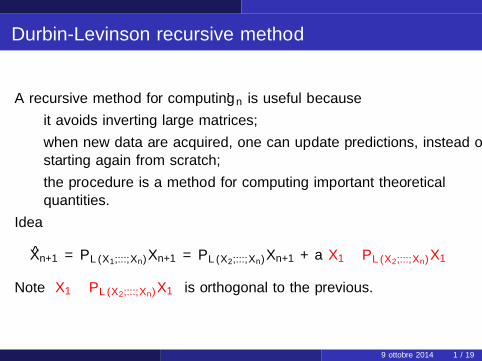
A recursive method for computing ϕn is useful because
it avoids inverting large matrices;
when new data are acquired, one can update predictions, instead ofstarting again from scratch;
the procedure is a method for computing important theoreticalquantities.
Idea
X̂n+1 = PL(X1,...,Xn)Xn+1 = PL(X2,...,Xn)Xn+1 + a(X1 − PL(X2,...,Xn)X1
)Note
(X1 − PL(X2,...,Xn)X1
)is orthogonal to the previous.
9 ottobre 2014 1 / 19
Durbin-Levinson recursive method
A recursive method for computing ϕn is useful because
it avoids inverting large matrices;
when new data are acquired, one can update predictions, instead ofstarting again from scratch;
the procedure is a method for computing important theoreticalquantities.
Idea
X̂n+1 = PL(X1,...,Xn)Xn+1 = PL(X2,...,Xn)Xn+1 + a(X1 − PL(X2,...,Xn)X1
)Note
(X1 − PL(X2,...,Xn)X1
)is orthogonal to the previous.
9 ottobre 2014 1 / 19
Durbin-Levinson, 2
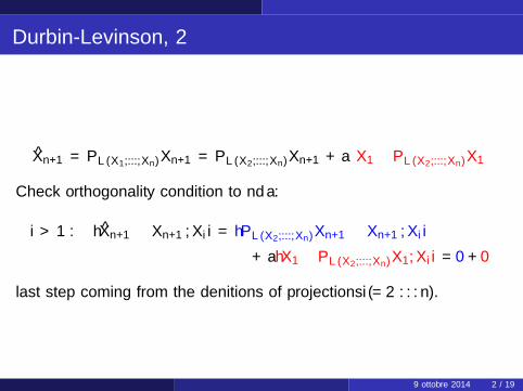
X̂n+1 = PL(X1,...,Xn)Xn+1 = PL(X2,...,Xn)Xn+1 + a(X1 − PL(X2,...,Xn)X1
)Check orthogonality condition to find a:
i > 1 : 〈X̂n+1 − Xn+1,Xi 〉 = 〈PL(X2,...,Xn)Xn+1 − Xn+1,Xi 〉+ a〈X1 − PL(X2,...,Xn)X1,Xi 〉 = 0 + 0
last step coming from the definitions of projections (i = 2 . . . n).
9 ottobre 2014 2 / 19
Durbin-Levinson, 3
X̂n+1 = PL(X1,...,Xn)Xn+1 = PL(X2,...,Xn)Xn+1 + a(X1 − PL(X2,...,Xn)X1
)Check orthogonality condition with i = 1:
0 = 〈X̂n+1 − Xn+1,X1 − PL(X2,...,Xn)X1〉= 〈PL(X2,...,Xn)Xn+1−Xn+1,X1−PL(X2,...,Xn)X1〉+ a‖X1−PL(X2,...,Xn)X1‖2
= −〈Xn+1,X1 − PL(X2,...,Xn)X1〉+ a‖X1 − PL(X2,...,Xn)X1‖2
=⇒ a =〈Xn+1,X1 − PL(X2,...,Xn)X1〉‖X1 − PL(X2,...,Xn)X1‖2
9 ottobre 2014 3 / 19
Durbin-Levinson, 3
X̂n+1 = PL(X1,...,Xn)Xn+1 = PL(X2,...,Xn)Xn+1 + a(X1 − PL(X2,...,Xn)X1
)Check orthogonality condition with i = 1:
0 = 〈X̂n+1 − Xn+1,X1 − PL(X2,...,Xn)X1〉
= 〈PL(X2,...,Xn)Xn+1−Xn+1,X1−PL(X2,...,Xn)X1〉+ a‖X1−PL(X2,...,Xn)X1‖2
= −〈Xn+1,X1 − PL(X2,...,Xn)X1〉+ a‖X1 − PL(X2,...,Xn)X1‖2
=⇒ a =〈Xn+1,X1 − PL(X2,...,Xn)X1〉‖X1 − PL(X2,...,Xn)X1‖2
9 ottobre 2014 3 / 19
Durbin-Levinson, 3
X̂n+1 = PL(X1,...,Xn)Xn+1 = PL(X2,...,Xn)Xn+1 + a(X1 − PL(X2,...,Xn)X1
)Check orthogonality condition with i = 1:
0 = 〈X̂n+1 − Xn+1,X1 − PL(X2,...,Xn)X1〉= 〈PL(X2,...,Xn)Xn+1−Xn+1,X1−PL(X2,...,Xn)X1〉+ a‖X1−PL(X2,...,Xn)X1‖2
= −〈Xn+1,X1 − PL(X2,...,Xn)X1〉+ a‖X1 − PL(X2,...,Xn)X1‖2
=⇒ a =〈Xn+1,X1 − PL(X2,...,Xn)X1〉‖X1 − PL(X2,...,Xn)X1‖2
9 ottobre 2014 3 / 19
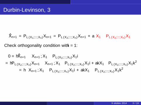
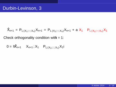
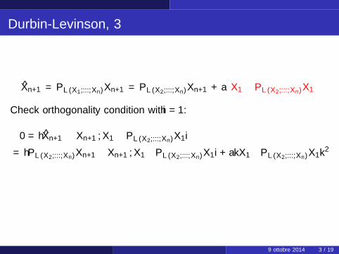
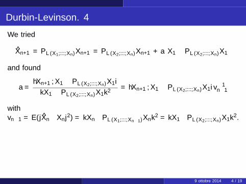
Durbin-Levinson. 4
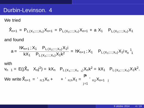
We tried
X̂n+1 = PL(X1,...,Xn)Xn+1 = PL(X2,...,Xn)Xn+1 + a(X1 − PL(X2,...,Xn)X1
)and found
a =〈Xn+1,X1 − PL(X2,...,Xn)X1〉‖X1 − PL(X2,...,Xn)X1‖2
= 〈Xn+1,X1 − PL(X2,...,Xn)X1〉v−1n−1
withvn−1 = E(|X̂n−Xn|2) = ‖Xn−PL(X1,...,Xn−1)Xn‖2 = ‖X1−PL(X2,...,Xn)X1‖2.
We write X̂n+1 = ϕn,1Xn + · · ·+ ϕn,nX1 =n∑
j=1ϕn,jXn+1−j
so that PL(X2,...,Xn)Xn+1 =n−1∑j=1
ϕn−1,jXn+1−j
and substituting we get a recursion.
9 ottobre 2014 4 / 19
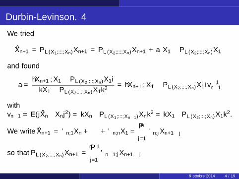
Durbin-Levinson. 4
We tried
X̂n+1 = PL(X1,...,Xn)Xn+1 = PL(X2,...,Xn)Xn+1 + a(X1 − PL(X2,...,Xn)X1
)and found
a =〈Xn+1,X1 − PL(X2,...,Xn)X1〉‖X1 − PL(X2,...,Xn)X1‖2
= 〈Xn+1,X1 − PL(X2,...,Xn)X1〉v−1n−1
withvn−1 = E(|X̂n−Xn|2) = ‖Xn−PL(X1,...,Xn−1)Xn‖2 = ‖X1−PL(X2,...,Xn)X1‖2.
We write X̂n+1 = ϕn,1Xn + · · ·+ ϕn,nX1 =n∑
j=1ϕn,jXn+1−j
so that PL(X2,...,Xn)Xn+1 =n−1∑j=1
ϕn−1,jXn+1−j
and substituting we get a recursion.
9 ottobre 2014 4 / 19
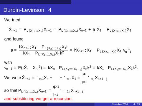
Durbin-Levinson. 4
We tried
X̂n+1 = PL(X1,...,Xn)Xn+1 = PL(X2,...,Xn)Xn+1 + a(X1 − PL(X2,...,Xn)X1
)and found
a =〈Xn+1,X1 − PL(X2,...,Xn)X1〉‖X1 − PL(X2,...,Xn)X1‖2
= 〈Xn+1,X1 − PL(X2,...,Xn)X1〉v−1n−1
withvn−1 = E(|X̂n−Xn|2) = ‖Xn−PL(X1,...,Xn−1)Xn‖2 = ‖X1−PL(X2,...,Xn)X1‖2.
We write X̂n+1 = ϕn,1Xn + · · ·+ ϕn,nX1 =n∑
j=1ϕn,jXn+1−j
so that PL(X2,...,Xn)Xn+1 =n−1∑j=1
ϕn−1,jXn+1−j
and substituting we get a recursion.9 ottobre 2014 4 / 19
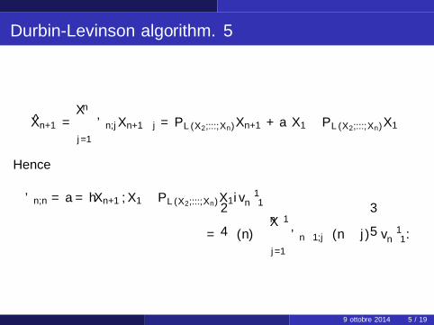
Durbin-Levinson algorithm. 5
X̂n+1 =n∑
j=1
ϕn,jXn+1−j = PL(X2,...,Xn)Xn+1 + a(X1 − PL(X2,...,Xn)X1
)Hence
ϕn,n = a = 〈Xn+1,X1 − PL(X2,...,Xn)X1〉v−1n−1
=
γ(n)−n−1∑j=1
ϕn−1,jγ(n − j)
v−1n−1.
9 ottobre 2014 5 / 19
Durbin-Levinson algorithm. 6
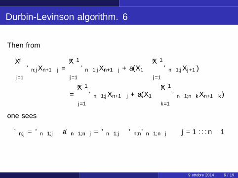
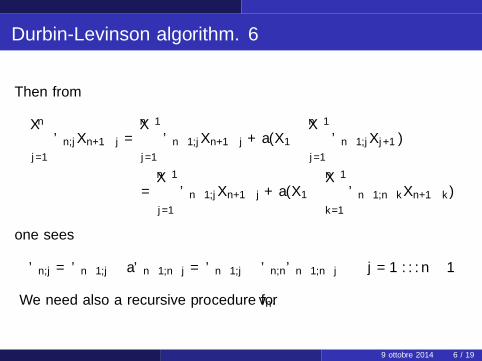
Then from
n∑j=1
ϕn,jXn+1−j =n−1∑j=1
ϕn−1,jXn+1−j + a(X1 −n−1∑j=1
ϕn−1,jXj+1)
=n−1∑j=1
ϕn−1,jXn+1−j + a(X1 −n−1∑k=1
ϕn−1,n−kXn+1−k)
one sees
ϕn,j = ϕn−1,j − aϕn−1,n−j = ϕn−1,j − ϕn,nϕn−1,n−j j = 1 . . . n − 1
We need also a recursive procedure for vn.
9 ottobre 2014 6 / 19
Durbin-Levinson algorithm. 6
Then from
n∑j=1
ϕn,jXn+1−j =n−1∑j=1
ϕn−1,jXn+1−j + a(X1 −n−1∑j=1
ϕn−1,jXj+1)
=n−1∑j=1
ϕn−1,jXn+1−j + a(X1 −n−1∑k=1
ϕn−1,n−kXn+1−k)
one sees
ϕn,j = ϕn−1,j − aϕn−1,n−j = ϕn−1,j − ϕn,nϕn−1,n−j j = 1 . . . n − 1
We need also a recursive procedure for vn.
9 ottobre 2014 6 / 19
Durbin-Levinson algorithm. 7
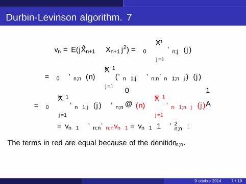
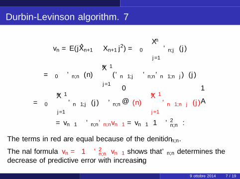
vn = E(|X̂n+1 − Xn+1|2) = γ0 −n∑
j=1
ϕn,jγ(j)
= γ0 − ϕn,nγ(n)−n−1∑j=1
(ϕn−1,j − ϕn,nϕn−1,n−j)γ(j)
= γ0 −n−1∑j=1
ϕn−1,jγ(j)− ϕn,n
γ(n)−n−1∑j=1
ϕn−1,n−jγ(j)
= vn−1 − ϕn,nϕn,nvn−1 = vn−1
(1− ϕ2
n,n
).
The terms in red are equal because of the definition ϕn,n.
The final formula vn =(1− ϕ2
n,n
)vn−1 shows that ϕn,n determines the
decrease of predictive error with increasing n.
9 ottobre 2014 7 / 19
Durbin-Levinson algorithm. 7
vn = E(|X̂n+1 − Xn+1|2) = γ0 −n∑
j=1
ϕn,jγ(j)
= γ0 − ϕn,nγ(n)−n−1∑j=1
(ϕn−1,j − ϕn,nϕn−1,n−j)γ(j)
= γ0 −n−1∑j=1
ϕn−1,jγ(j)− ϕn,n
γ(n)−n−1∑j=1
ϕn−1,n−jγ(j)
= vn−1 − ϕn,nϕn,nvn−1 = vn−1
(1− ϕ2
n,n
).
The terms in red are equal because of the definition ϕn,n.
The final formula vn =(1− ϕ2
n,n
)vn−1 shows that ϕn,n determines the
decrease of predictive error with increasing n.
9 ottobre 2014 7 / 19
Durbin-Levinson algorithm. Summary
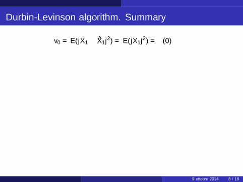
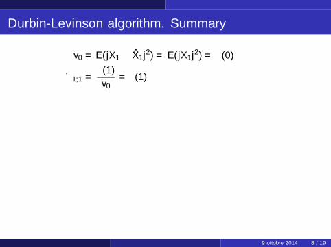
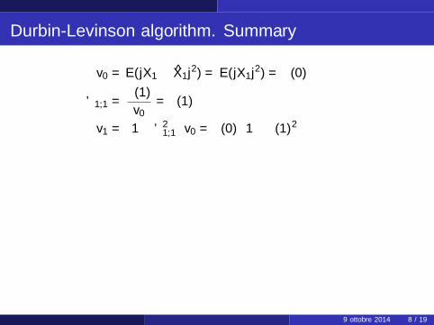
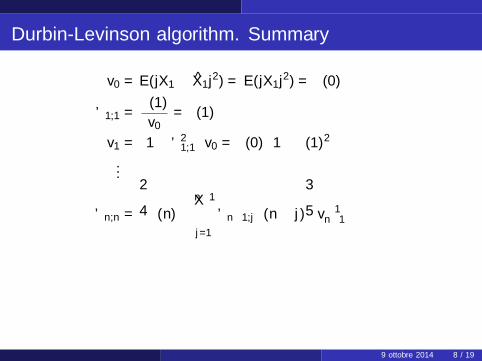
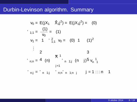
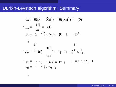
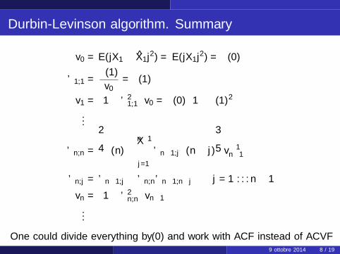
v0 = E(|X1 − X̂1|2) = E(|X1|2) = γ(0)
ϕ1,1 =γ(1)
v0= ρ(1)
v1 =(1− ϕ2
1,1
)v0 = γ(0)
(1− ρ(1)2
)...
ϕn,n =
γ(n)−n−1∑j=1
ϕn−1,jγ(n − j)
v−1n−1
ϕn,j = ϕn−1,j − ϕn,nϕn−1,n−j j = 1 . . . n − 1
vn =(1− ϕ2
n,n
)vn−1
...
One could divide everything by γ(0) and work with ACF instead of ACVF
9 ottobre 2014 8 / 19
Durbin-Levinson algorithm. Summary
v0 = E(|X1 − X̂1|2) = E(|X1|2) = γ(0)
ϕ1,1 =γ(1)
v0= ρ(1)
v1 =(1− ϕ2
1,1
)v0 = γ(0)
(1− ρ(1)2
)
...
ϕn,n =
γ(n)−n−1∑j=1
ϕn−1,jγ(n − j)
v−1n−1
ϕn,j = ϕn−1,j − ϕn,nϕn−1,n−j j = 1 . . . n − 1
vn =(1− ϕ2
n,n
)vn−1
...
One could divide everything by γ(0) and work with ACF instead of ACVF
9 ottobre 2014 8 / 19
Durbin-Levinson algorithm. Summary
v0 = E(|X1 − X̂1|2) = E(|X1|2) = γ(0)
ϕ1,1 =γ(1)
v0= ρ(1)
v1 =(1− ϕ2
1,1
)v0 = γ(0)
(1− ρ(1)2
)...
ϕn,n =
γ(n)−n−1∑j=1
ϕn−1,jγ(n − j)
v−1n−1
ϕn,j = ϕn−1,j − ϕn,nϕn−1,n−j j = 1 . . . n − 1
vn =(1− ϕ2
n,n
)vn−1
...
One could divide everything by γ(0) and work with ACF instead of ACVF
9 ottobre 2014 8 / 19
Durbin-Levinson algorithm. Summary
v0 = E(|X1 − X̂1|2) = E(|X1|2) = γ(0)
ϕ1,1 =γ(1)
v0= ρ(1)
v1 =(1− ϕ2
1,1
)v0 = γ(0)
(1− ρ(1)2
)...
ϕn,n =
γ(n)−n−1∑j=1
ϕn−1,jγ(n − j)
v−1n−1
ϕn,j = ϕn−1,j − ϕn,nϕn−1,n−j j = 1 . . . n − 1
vn =(1− ϕ2
n,n
)vn−1
...
One could divide everything by γ(0) and work with ACF instead of ACVF9 ottobre 2014 8 / 19
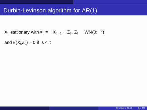
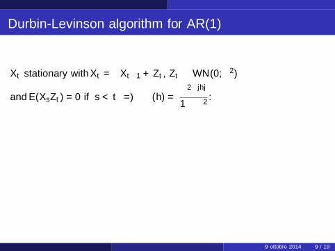
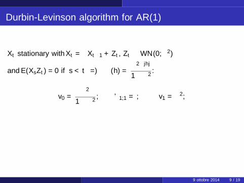
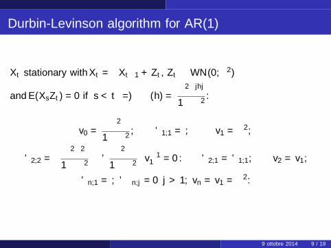
Durbin-Levinson algorithm for AR(1)
Xt stationary with Xt = φXt−1 + Zt , Zt ∼WN(0, σ2)
and E(XsZt) = 0 if s < t
=⇒ γ(h) =σ2φ|h|
1− φ2.
v0 =σ2
1− φ2, ϕ1,1 = φ, v1 = σ2,
ϕ2,2 =
[σ2φ2
1− φ2− ϕ σ2φ
1− φ2
]v−11 = 0. ϕ2,1 = ϕ1,1, v2 = v1,
ϕn,1 = φ, ϕn,j = 0 j > 1, vn = v1 = σ2.
9 ottobre 2014 9 / 19
Durbin-Levinson algorithm for AR(1)
Xt stationary with Xt = φXt−1 + Zt , Zt ∼WN(0, σ2)
and E(XsZt) = 0 if s < t =⇒ γ(h) =σ2φ|h|
1− φ2.
v0 =σ2
1− φ2, ϕ1,1 = φ, v1 = σ2,
ϕ2,2 =
[σ2φ2
1− φ2− ϕ σ2φ
1− φ2
]v−11 = 0. ϕ2,1 = ϕ1,1, v2 = v1,
ϕn,1 = φ, ϕn,j = 0 j > 1, vn = v1 = σ2.
9 ottobre 2014 9 / 19
Durbin-Levinson algorithm for AR(1)
Xt stationary with Xt = φXt−1 + Zt , Zt ∼WN(0, σ2)
and E(XsZt) = 0 if s < t =⇒ γ(h) =σ2φ|h|
1− φ2.
v0 =σ2
1− φ2, ϕ1,1 = φ, v1 = σ2,
ϕ2,2 =
[σ2φ2
1− φ2− ϕ σ2φ
1− φ2
]v−11 = 0. ϕ2,1 = ϕ1,1, v2 = v1,
ϕn,1 = φ, ϕn,j = 0 j > 1, vn = v1 = σ2.
9 ottobre 2014 9 / 19
Durbin-Levinson algorithm for AR(1)
Xt stationary with Xt = φXt−1 + Zt , Zt ∼WN(0, σ2)
and E(XsZt) = 0 if s < t =⇒ γ(h) =σ2φ|h|
1− φ2.
v0 =σ2
1− φ2, ϕ1,1 = φ, v1 = σ2,
ϕ2,2 =
[σ2φ2
1− φ2− ϕ σ2φ
1− φ2
]v−11 = 0. ϕ2,1 = ϕ1,1, v2 = v1,
ϕn,1 = φ, ϕn,j = 0 j > 1, vn = v1 = σ2.
9 ottobre 2014 9 / 19
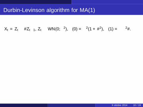
Durbin-Levinson algorithm for MA(1)
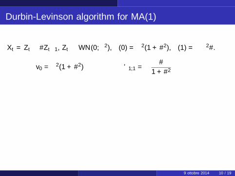
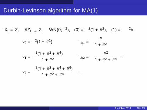
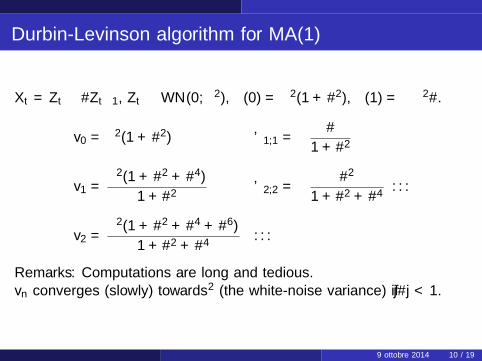
Xt = Zt − ϑZt−1, Zt ∼WN(0, σ2), γ(0) = σ2(1 + ϑ2), γ(1) = −σ2ϑ.
v0 = σ2(1 + ϑ2) ϕ1,1 = − ϑ
1 + ϑ2
v1 =σ2(1 + ϑ2 + ϑ4)
1 + ϑ2ϕ2,2 = − ϑ2
1 + ϑ2 + ϑ4. . .
v2 =σ2(1 + ϑ2 + ϑ4 + ϑ6)
1 + ϑ2 + ϑ4. . .
Remarks: Computations are long and tedious.vn converges (slowly) towards σ2 (the white-noise variance) if |ϑ| < 1.
9 ottobre 2014 10 / 19
Durbin-Levinson algorithm for MA(1)
Xt = Zt − ϑZt−1, Zt ∼WN(0, σ2), γ(0) = σ2(1 + ϑ2), γ(1) = −σ2ϑ.
v0 = σ2(1 + ϑ2) ϕ1,1 = − ϑ
1 + ϑ2
v1 =σ2(1 + ϑ2 + ϑ4)
1 + ϑ2ϕ2,2 = − ϑ2
1 + ϑ2 + ϑ4. . .
v2 =σ2(1 + ϑ2 + ϑ4 + ϑ6)
1 + ϑ2 + ϑ4. . .
Remarks: Computations are long and tedious.vn converges (slowly) towards σ2 (the white-noise variance) if |ϑ| < 1.
9 ottobre 2014 10 / 19
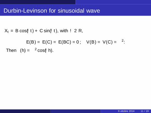
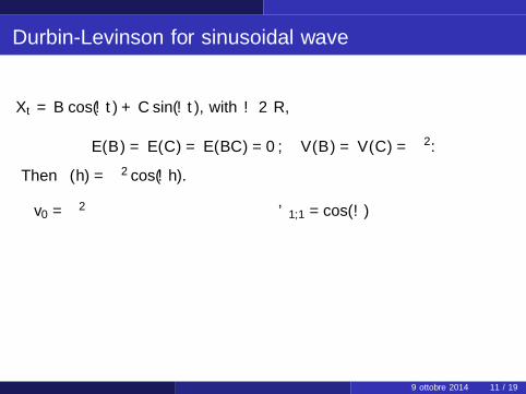
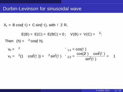
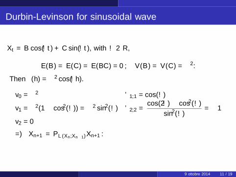
Durbin-Levinson for sinusoidal wave
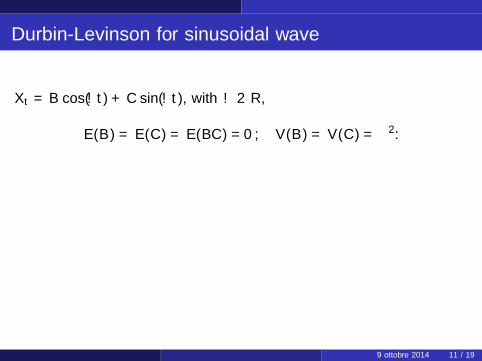
Xt = B cos(ωt) + C sin(ωt), with ω ∈ R,
E(B) = E(C ) = E(BC ) = 0, V(B) = V(C ) = σ2.
Then γ(h) = σ2 cos(ωh).
v0 = σ2 ϕ1,1 = cos(ω)
v1 = σ2(1− cos2(ω)) = σ2 sin2(ω) ϕ2,2 =cos(2ω)− cos2(ω)
sin2(ω)= −1
v2 = 0
=⇒ Xn+1 = PL(Xn,Xn−1)Xn+1.
9 ottobre 2014 11 / 19
Durbin-Levinson for sinusoidal wave
Xt = B cos(ωt) + C sin(ωt), with ω ∈ R,
E(B) = E(C ) = E(BC ) = 0, V(B) = V(C ) = σ2.
Then γ(h) = σ2 cos(ωh).
v0 = σ2 ϕ1,1 = cos(ω)
v1 = σ2(1− cos2(ω)) = σ2 sin2(ω) ϕ2,2 =cos(2ω)− cos2(ω)
sin2(ω)= −1
v2 = 0
=⇒ Xn+1 = PL(Xn,Xn−1)Xn+1.
9 ottobre 2014 11 / 19
Durbin-Levinson for sinusoidal wave
Xt = B cos(ωt) + C sin(ωt), with ω ∈ R,
E(B) = E(C ) = E(BC ) = 0, V(B) = V(C ) = σ2.
Then γ(h) = σ2 cos(ωh).
v0 = σ2 ϕ1,1 = cos(ω)
v1 = σ2(1− cos2(ω)) = σ2 sin2(ω) ϕ2,2 =cos(2ω)− cos2(ω)
sin2(ω)= −1
v2 = 0
=⇒ Xn+1 = PL(Xn,Xn−1)Xn+1.
9 ottobre 2014 11 / 19
Durbin-Levinson for sinusoidal wave
Xt = B cos(ωt) + C sin(ωt), with ω ∈ R,
E(B) = E(C ) = E(BC ) = 0, V(B) = V(C ) = σ2.
Then γ(h) = σ2 cos(ωh).
v0 = σ2 ϕ1,1 = cos(ω)
v1 = σ2(1− cos2(ω)) = σ2 sin2(ω) ϕ2,2 =cos(2ω)− cos2(ω)
sin2(ω)= −1
v2 = 0
=⇒ Xn+1 = PL(Xn,Xn−1)Xn+1.
9 ottobre 2014 11 / 19
Durbin-Levinson for sinusoidal wave
Xt = B cos(ωt) + C sin(ωt), with ω ∈ R,
E(B) = E(C ) = E(BC ) = 0, V(B) = V(C ) = σ2.
Then γ(h) = σ2 cos(ωh).
v0 = σ2 ϕ1,1 = cos(ω)
v1 = σ2(1− cos2(ω)) = σ2 sin2(ω) ϕ2,2 =cos(2ω)− cos2(ω)
sin2(ω)= −1
v2 = 0
=⇒ Xn+1 = PL(Xn,Xn−1)Xn+1.
9 ottobre 2014 11 / 19
Partial auto-correlation
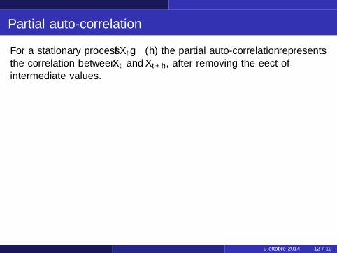
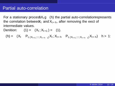
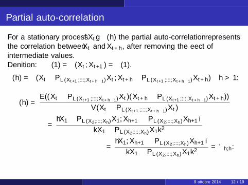
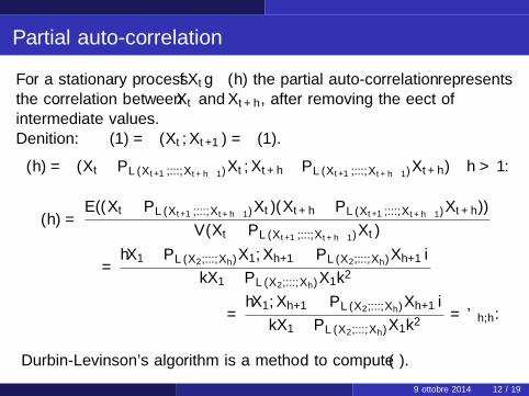
For a stationary process {Xt} α(h) the partial auto-correlation representsthe correlation between Xt and Xt+h, after removing the effect ofintermediate values.
Definition: α(1) = ρ(Xt ,Xt+1) = ρ(1).
α(h) = ρ(Xt −PL(Xt+1,...,Xt+h−1)Xt ,Xt+h−PL(Xt+1,...,Xt+h−1)Xt+h) h > 1.
α(h) =E((Xt − PL(Xt+1,...,Xt+h−1)Xt)(Xt+h − PL(Xt+1,...,Xt+h−1)Xt+h))
V(Xt − PL(Xt+1,...,Xt+h−1)Xt)
=〈X1 − PL(X2,...,Xh)X1,Xh+1 − PL(X2,...,Xh)Xh+1〉
‖X1 − PL(X2,...,Xh)X1‖2
=〈X1,Xh+1 − PL(X2,...,Xh)Xh+1〉‖X1 − PL(X2,...,Xh)X1‖2
= ϕh,h.
Durbin-Levinson’s algorithm is a method to compute α(·).
9 ottobre 2014 12 / 19
Partial auto-correlation
For a stationary process {Xt} α(h) the partial auto-correlation representsthe correlation between Xt and Xt+h, after removing the effect ofintermediate values.Definition: α(1) = ρ(Xt ,Xt+1) = ρ(1).
α(h) = ρ(Xt −PL(Xt+1,...,Xt+h−1)Xt ,Xt+h−PL(Xt+1,...,Xt+h−1)Xt+h) h > 1.
α(h) =E((Xt − PL(Xt+1,...,Xt+h−1)Xt)(Xt+h − PL(Xt+1,...,Xt+h−1)Xt+h))
V(Xt − PL(Xt+1,...,Xt+h−1)Xt)
=〈X1 − PL(X2,...,Xh)X1,Xh+1 − PL(X2,...,Xh)Xh+1〉
‖X1 − PL(X2,...,Xh)X1‖2
=〈X1,Xh+1 − PL(X2,...,Xh)Xh+1〉‖X1 − PL(X2,...,Xh)X1‖2
= ϕh,h.
Durbin-Levinson’s algorithm is a method to compute α(·).
9 ottobre 2014 12 / 19
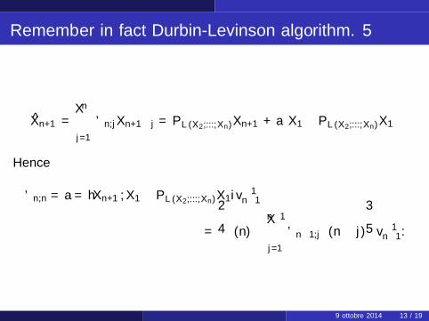
Remember in fact Durbin-Levinson algorithm. 5
X̂n+1 =n∑
j=1
ϕn,jXn+1−j = PL(X2,...,Xn)Xn+1 + a(X1 − PL(X2,...,Xn)X1
)Hence
ϕn,n = a = 〈Xn+1,X1 − PL(X2,...,Xn)X1〉v−1n−1
=
γ(n)−n−1∑j=1
ϕn−1,jγ(n − j)
v−1n−1.
9 ottobre 2014 13 / 19
Examples of PACF
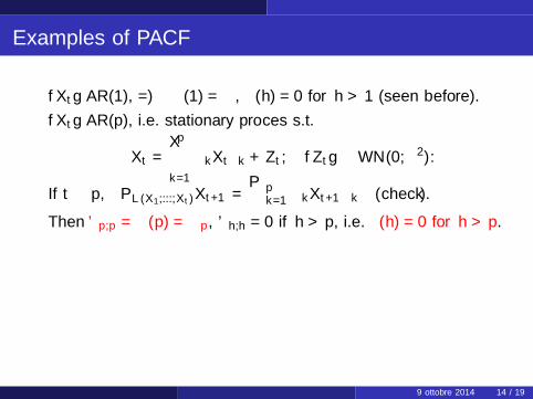
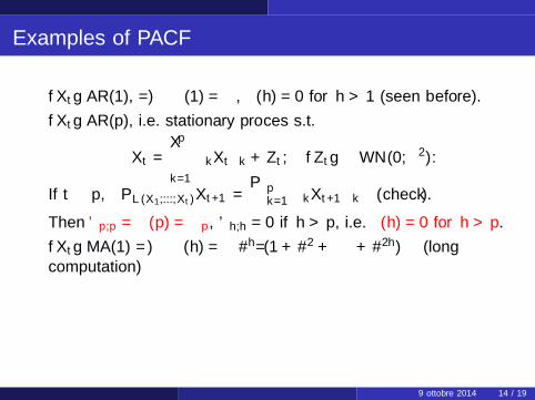
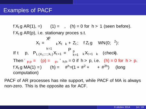
{Xt} AR(1), =⇒ α(1) = φ, α(h) = 0 for h > 1 (seen before).
{Xt} AR(p), i.e. stationary proces s.t.
Xt =
p∑k=1
φkXt−k + Zt , {Zt} ∼WN(0, σ2).
If t ≥ p, PL(X1,...,Xt)Xt+1 =∑p
k=1 φkXt+1−k (check).
Then ϕp,p = α(p) = φp, ϕh,h = 0 if h > p, i.e. α(h) = 0 for h > p.
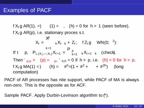
{Xt} MA(1) =⇒ α(h) = −ϑh/(1 + ϑ2 + · · ·+ ϑ2h) (longcomputation)
PACF of AR processes has finite support, while PACF of MA is alwaysnon-zero. This is the opposite as for ACF.
Sample PACF. Apply Durbin-Levinson algorithm to γ̂(·).
9 ottobre 2014 14 / 19
Examples of PACF
{Xt} AR(1), =⇒ α(1) = φ, α(h) = 0 for h > 1 (seen before).
{Xt} AR(p), i.e. stationary proces s.t.
Xt =
p∑k=1
φkXt−k + Zt , {Zt} ∼WN(0, σ2).
If t ≥ p, PL(X1,...,Xt)Xt+1 =∑p
k=1 φkXt+1−k (check).
Then ϕp,p = α(p) = φp, ϕh,h = 0 if h > p, i.e. α(h) = 0 for h > p.
{Xt} MA(1) =⇒ α(h) = −ϑh/(1 + ϑ2 + · · ·+ ϑ2h) (longcomputation)
PACF of AR processes has finite support, while PACF of MA is alwaysnon-zero. This is the opposite as for ACF.
Sample PACF. Apply Durbin-Levinson algorithm to γ̂(·).
9 ottobre 2014 14 / 19

Sample ACF and PACF
0 5 10 15
-0.5
0.0
0.5
1.0
Lag
ACF
Oveshort data
5 10 15
-0.4
0.0
0.2
Lag
Par
tial A
CF
9 ottobre 2014 15 / 19

Sample ACF of Huron: AR(1) fit
0 5 10 15
-0.4
-0.2
0.0
0.2
0.4
0.6
0.8
1.0
Lag
ACF
ACF of detrended Huron data
9 ottobre 2014 16 / 19
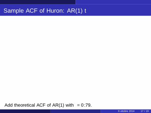
Sample ACF of Huron: AR(1) fit
0 5 10 15
-0.4
-0.2
0.0
0.2
0.4
0.6
0.8
1.0
Lag
ACF
ACF of detrended Huron data
Add theoretical ACF of AR(1) with φ = 0.79.9 ottobre 2014 17 / 19
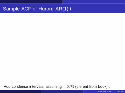
Sample ACF of Huron: AR(1) fit
0 5 10 15
-0.4
-0.2
0.0
0.2
0.4
0.6
0.8
1.0
Lag
ACF
ACF of detrended Huron data
Add confidence intervals, assuming φ = 0.79 (different from book).9 ottobre 2014 18 / 19
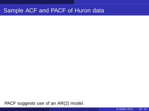
Sample ACF and PACF of Huron data
0 5 10 15
-0.2
0.2
0.6
1.0
Lag
ACF
Huron data
5 10 15
-0.2
0.2
0.6
Lag
Par
tial A
CF
PACF suggests use of an AR(2) model.9 ottobre 2014 19 / 19