dsp system toolbox™ user’s guide
DESCRIPTION
DSP System Toolbox™ User’s GuideTRANSCRIPT

DSP System Toolbox™
User’s Guide
R2014a
How to Contact MathWorks
www.mathworks.com Webcomp.soft-sys.matlab Newsgroupwww.mathworks.com/contact_TS.html Technical Support
[email protected] Product enhancement [email protected] Bug [email protected] Documentation error [email protected] Order status, license renewals, [email protected] Sales, pricing, and general information
508-647-7000 (Phone)
508-647-7001 (Fax)
The MathWorks, Inc.3 Apple Hill DriveNatick, MA 01760-2098For contact information about worldwide offices, see the MathWorks Web site.
DSP System Toolbox™ User’s Guide
© COPYRIGHT 2011–2014 by The MathWorks, Inc.The software described in this document is furnished under a license agreement. The software may be usedor copied only under the terms of the license agreement. No part of this manual may be photocopied orreproduced in any form without prior written consent from The MathWorks, Inc.
FEDERAL ACQUISITION: This provision applies to all acquisitions of the Program and Documentationby, for, or through the federal government of the United States. By accepting delivery of the Programor Documentation, the government hereby agrees that this software or documentation qualifies ascommercial computer software or commercial computer software documentation as such terms are usedor defined in FAR 12.212, DFARS Part 227.72, and DFARS 252.227-7014. Accordingly, the terms andconditions of this Agreement and only those rights specified in this Agreement, shall pertain to and governthe use, modification, reproduction, release, performance, display, and disclosure of the Program andDocumentation by the federal government (or other entity acquiring for or through the federal government)and shall supersede any conflicting contractual terms or conditions. If this License fails to meet thegovernment’s needs or is inconsistent in any respect with federal procurement law, the government agreesto return the Program and Documentation, unused, to The MathWorks, Inc.
Trademarks
MATLAB and Simulink are registered trademarks of The MathWorks, Inc. Seewww.mathworks.com/trademarks for a list of additional trademarks. Other product or brandnames may be trademarks or registered trademarks of their respective holders.
Patents
MathWorks products are protected by one or more U.S. patents. Please seewww.mathworks.com/patents for more information.

Revision HistoryApril 2011 First printing Revised for Version 8.0 (R2011a)September 2011 Online only Revised for Version 8.1 (R2011b)March 2012 Online only Revised for Version 8.2 (R2012a)September 2012 Online only Revised for Version 8.3 (R2012b)March 2013 Online only Revised for Version 8.4 (R2013a)September 2013 Online only Revised for Version 8.5 (R2013b)March 2014 Online only Revised for Version 8.6 (R2014a)


Contents
Input, Output, and Display
1Discrete-Time Signals . . . . . . . . . . . . . . . . . . . . . . . . . . . . . . 1-2Time and Frequency Terminology . . . . . . . . . . . . . . . . . . . . 1-2Recommended Settings for Discrete-Time Simulations . . . 1-4Other Settings for Discrete-Time Simulations . . . . . . . . . . 1-6
Continuous-Time Signals . . . . . . . . . . . . . . . . . . . . . . . . . . . 1-11Continuous-Time Source Blocks . . . . . . . . . . . . . . . . . . . . . . 1-11Continuous-Time Nonsource Blocks . . . . . . . . . . . . . . . . . . 1-11
Create Sample-Based Signals . . . . . . . . . . . . . . . . . . . . . . . 1-13Create Signals Using Constant Block . . . . . . . . . . . . . . . . . 1-13Create Signals Using Signal from Workspace Block . . . . . 1-16
Create Frame-Based Signals . . . . . . . . . . . . . . . . . . . . . . . . 1-19Create Signals Using Sine Wave Block . . . . . . . . . . . . . . . . 1-19Create Signals Using Signal from Workspace Block . . . . . 1-22
Create Multichannel Sample-Based Signals . . . . . . . . . . 1-26Multichannel Sample-Based Signals . . . . . . . . . . . . . . . . . . 1-26Create Multichannel Signals by Combining Single-ChannelSignals . . . . . . . . . . . . . . . . . . . . . . . . . . . . . . . . . . . . . . . . 1-26
Create Multichannel Signals by Combining MultichannelSignals . . . . . . . . . . . . . . . . . . . . . . . . . . . . . . . . . . . . . . . . 1-29
Create Multichannel Frame-Based Signals . . . . . . . . . . . 1-32Multichannel Frame-Based Signals . . . . . . . . . . . . . . . . . . . 1-32Create Multichannel Signals Using Concatenate Block . . . 1-33
Deconstruct Multichannel Sample-Based Signals . . . . . 1-36Split Multichannel Signals into Individual Signals . . . . . . 1-36Split Multichannel Signals into Several MultichannelSignals . . . . . . . . . . . . . . . . . . . . . . . . . . . . . . . . . . . . . . . . 1-39
v
Deconstruct Multichannel Frame-Based Signals . . . . . . 1-43Split Multichannel Signals into Individual Signals . . . . . . 1-43Reorder Channels in Multichannel Frame-BasedSignals . . . . . . . . . . . . . . . . . . . . . . . . . . . . . . . . . . . . . . . . 1-48
Import and Export Sample-Based Signals . . . . . . . . . . . . 1-52Import Sample-Based Vector Signals . . . . . . . . . . . . . . . . . 1-52Import Sample-Based Matrix Signals . . . . . . . . . . . . . . . . . 1-56Export Sample-Based Signals . . . . . . . . . . . . . . . . . . . . . . . 1-59
Import and Export Frame-Based Signals . . . . . . . . . . . . . 1-64Import Frame-Based Signals . . . . . . . . . . . . . . . . . . . . . . . . 1-64Export Frame-Based Signals . . . . . . . . . . . . . . . . . . . . . . . . 1-67
Musical Instrument Digital Interface . . . . . . . . . . . . . . . . 1-72About MIDI . . . . . . . . . . . . . . . . . . . . . . . . . . . . . . . . . . . . . . 1-72MIDI Control Surfaces . . . . . . . . . . . . . . . . . . . . . . . . . . . . . 1-72Using MIDI Control Surfaces with MATLAB andSimulink . . . . . . . . . . . . . . . . . . . . . . . . . . . . . . . . . . . . . . 1-73
Display Time-Domain Data . . . . . . . . . . . . . . . . . . . . . . . . . 1-77Configure the Time Scope Properties . . . . . . . . . . . . . . . . . . 1-78Use the Simulation Controls . . . . . . . . . . . . . . . . . . . . . . . . 1-85Modify the Time Scope Display . . . . . . . . . . . . . . . . . . . . . . 1-86Inspect Your Data (Scaling the Axes and Zooming) . . . . . . 1-88Manage Multiple Time Scopes . . . . . . . . . . . . . . . . . . . . . . . 1-91
Display Frequency-Domain Data in SpectrumAnalyzer . . . . . . . . . . . . . . . . . . . . . . . . . . . . . . . . . . . . . . . . 1-96
Visualize Central Limit Theorem in Array Plot . . . . . . . 1-104Display a Uniform Distribution . . . . . . . . . . . . . . . . . . . . . . 1-104Display the Sum of Many Uniform Distributions . . . . . . . . 1-105Inspect Your Data by Zooming . . . . . . . . . . . . . . . . . . . . . . . 1-107
vi Contents
Data and Signal Management
2Sample- and Frame-Based Concepts . . . . . . . . . . . . . . . . . 2-2Sample- and Frame-Based Signals . . . . . . . . . . . . . . . . . . . 2-2Model Sample- and Frame-Based Signals in MATLAB andSimulink . . . . . . . . . . . . . . . . . . . . . . . . . . . . . . . . . . . . . . 2-3
What Is Sample-Based Processing? . . . . . . . . . . . . . . . . . . . 2-4What Is Frame-Based Processing? . . . . . . . . . . . . . . . . . . . . 2-5
Inspect Sample and Frame Rates in Simulink . . . . . . . . 2-8Sample Rate and Frame Rate Concepts . . . . . . . . . . . . . . . 2-8Inspect Sample-Based Signals Using Probe Block . . . . . . . 2-10Inspect Frame-Based Signals Using Probe Block . . . . . . . . 2-12Inspect Sample-Based Signals Using Color Coding . . . . . . 2-15Inspect Frame-Based Signals Using Color Coding . . . . . . . 2-16
Convert Sample and Frame Rates in Simulink . . . . . . . 2-20Rate Conversion Blocks . . . . . . . . . . . . . . . . . . . . . . . . . . . . 2-20Rate Conversion by Frame-Rate Adjustment . . . . . . . . . . . 2-21Rate Conversion by Frame-Size Adjustment . . . . . . . . . . . . 2-25Avoid Unintended Rate Conversion . . . . . . . . . . . . . . . . . . . 2-29Frame Rebuffering Blocks . . . . . . . . . . . . . . . . . . . . . . . . . . 2-35Buffer Signals by Preserving the Sample Period . . . . . . . . 2-38Buffer Signals by Altering the Sample Period . . . . . . . . . . 2-41
Buffering and Frame-Based Processing . . . . . . . . . . . . . . 2-45Frame Status . . . . . . . . . . . . . . . . . . . . . . . . . . . . . . . . . . . . . 2-45Buffer Sample-Based Signals into Frame-Based Signals . . 2-45Buffer Sample-Based Signals into Frame-Based Signalswith Overlap . . . . . . . . . . . . . . . . . . . . . . . . . . . . . . . . . . . 2-49
Buffer Frame-Based Signals into Other Frame-BasedSignals . . . . . . . . . . . . . . . . . . . . . . . . . . . . . . . . . . . . . . . . 2-53
Buffer Delay and Initial Conditions . . . . . . . . . . . . . . . . . . . 2-56Unbuffer Frame-Based Signals into Sample-BasedSignals . . . . . . . . . . . . . . . . . . . . . . . . . . . . . . . . . . . . . . . . 2-57
Delay and Latency . . . . . . . . . . . . . . . . . . . . . . . . . . . . . . . . . 2-61Computational Delay . . . . . . . . . . . . . . . . . . . . . . . . . . . . . . 2-61Algorithmic Delay . . . . . . . . . . . . . . . . . . . . . . . . . . . . . . . . . 2-63Zero Algorithmic Delay . . . . . . . . . . . . . . . . . . . . . . . . . . . . . 2-63
vii

Basic Algorithmic Delay . . . . . . . . . . . . . . . . . . . . . . . . . . . . 2-66Excess Algorithmic Delay (Tasking Latency) . . . . . . . . . . . 2-70Predict Tasking Latency . . . . . . . . . . . . . . . . . . . . . . . . . . . . 2-72
Filter Analysis, Design, and Implementation
3Design a Filter in Fdesign — Process Overview . . . . . . 3-2Process Flow Diagram and Filter Design Methodology . . . 3-2
Design a Filter in the Filterbuilder GUI . . . . . . . . . . . . . 3-11The Graphical Interface to Fdesign . . . . . . . . . . . . . . . . . . . 3-11
Use FDATool with DSP System Toolbox Software . . . . 3-16Design Advanced Filters in FDATool . . . . . . . . . . . . . . . . . . 3-16Access the Quantization Features of FDATool . . . . . . . . . . 3-21Quantize Filters in FDATool . . . . . . . . . . . . . . . . . . . . . . . . 3-23Analyze Filters with a Noise-Based Method . . . . . . . . . . . . 3-31Scale Second-Order Section Filters . . . . . . . . . . . . . . . . . . . 3-38Reorder the Sections of Second-Order Section Filters . . . . 3-43View SOS Filter Sections . . . . . . . . . . . . . . . . . . . . . . . . . . . 3-49Import and Export Quantized Filters . . . . . . . . . . . . . . . . . 3-54Generate MATLAB Code . . . . . . . . . . . . . . . . . . . . . . . . . . . 3-59Import XILINX Coefficient (.COE) Files . . . . . . . . . . . . . . . 3-60Transform Filters Using FDATool . . . . . . . . . . . . . . . . . . . . 3-60Design Multirate Filters in FDATool . . . . . . . . . . . . . . . . . . 3-70Realize Filters as Simulink Subsystem Blocks . . . . . . . . . . 3-84
Digital Frequency Transformations . . . . . . . . . . . . . . . . . 3-88Details and Methodology . . . . . . . . . . . . . . . . . . . . . . . . . . . 3-88Frequency Transformations for Real Filters . . . . . . . . . . . . 3-96Frequency Transformations for Complex Filters . . . . . . . . 3-110
Digital Filter Design Block . . . . . . . . . . . . . . . . . . . . . . . . . 3-123Overview of the Digital Filter Design Block . . . . . . . . . . . . 3-123Select a Filter Design Block . . . . . . . . . . . . . . . . . . . . . . . . . 3-124Create a Lowpass Filter in Simulink . . . . . . . . . . . . . . . . . . 3-126Create a Highpass Filter in Simulink . . . . . . . . . . . . . . . . . 3-127Filter High-Frequency Noise in Simulink . . . . . . . . . . . . . . 3-128
viii Contents

Filter Realization Wizard . . . . . . . . . . . . . . . . . . . . . . . . . . . 3-134Overview of the Filter Realization Wizard . . . . . . . . . . . . . 3-134Design and Implement a Fixed-Point Filter in Simulink . . 3-134Set the Filter Structure and Number of Filter Sections . . . 3-143Optimize the Filter Structure . . . . . . . . . . . . . . . . . . . . . . . . 3-144
Digital Filter Block . . . . . . . . . . . . . . . . . . . . . . . . . . . . . . . . 3-147Overview of the Digital Filter Block . . . . . . . . . . . . . . . . . . 3-147Implement a Lowpass Filter in Simulink . . . . . . . . . . . . . . 3-148Implement a Highpass Filter in Simulink . . . . . . . . . . . . . . 3-149Filter High-Frequency Noise in Simulink . . . . . . . . . . . . . . 3-150Specify Static Filters . . . . . . . . . . . . . . . . . . . . . . . . . . . . . . . 3-155Specify Time-Varying Filters . . . . . . . . . . . . . . . . . . . . . . . . 3-155Specify the SOS Matrix (Biquadratic Filter Coefficients) . . 3-157
Analog Filter Design Block . . . . . . . . . . . . . . . . . . . . . . . . . 3-159
Adaptive Filters
4Overview of Adaptive Filters and Applications . . . . . . . 4-2Introduction to Adaptive Filtering . . . . . . . . . . . . . . . . . . . . 4-2Adaptive Filtering Methodology . . . . . . . . . . . . . . . . . . . . . . 4-2Choosing an Adaptive Filter . . . . . . . . . . . . . . . . . . . . . . . . . 4-4System Identification . . . . . . . . . . . . . . . . . . . . . . . . . . . . . . 4-6Inverse System Identification . . . . . . . . . . . . . . . . . . . . . . . . 4-6Noise or Interference Cancellation . . . . . . . . . . . . . . . . . . . . 4-7Prediction . . . . . . . . . . . . . . . . . . . . . . . . . . . . . . . . . . . . . . . . 4-8
Adaptive Filters in DSP System Toolbox Software . . . . 4-10Overview of Adaptive Filtering in DSP System ToolboxSoftware . . . . . . . . . . . . . . . . . . . . . . . . . . . . . . . . . . . . . . . 4-10
Algorithms . . . . . . . . . . . . . . . . . . . . . . . . . . . . . . . . . . . . . . . 4-10Using Adaptive Filter Objects . . . . . . . . . . . . . . . . . . . . . . . 4-13
LMS Adaptive Filters . . . . . . . . . . . . . . . . . . . . . . . . . . . . . . 4-14LMS Methods for adaptfilt Objects . . . . . . . . . . . . . . . . . . . 4-14System Identification Using adaptfilt.lms . . . . . . . . . . . . . . 4-16System Identification Using adaptfilt.nlms . . . . . . . . . . . . . 4-19
ix

Noise Cancellation Using adaptfilt.sd . . . . . . . . . . . . . . . . . 4-22Noise Cancellation Using adaptfilt.se . . . . . . . . . . . . . . . . . 4-26Noise Cancellation Using adaptfilt.ss . . . . . . . . . . . . . . . . . 4-30
RLS Adaptive Filters . . . . . . . . . . . . . . . . . . . . . . . . . . . . . . . 4-35Compare RLS and LMS Adaptive Filter Algorithms . . . . . 4-35Inverse System Identification Using adaptfilt.rls . . . . . . . . 4-36
Signal Enhancement Using LMS and NormalizedLMS . . . . . . . . . . . . . . . . . . . . . . . . . . . . . . . . . . . . . . . . . . . . 4-41Create the Signals for Adaptation . . . . . . . . . . . . . . . . . . . . 4-41Construct Two Adaptive Filters . . . . . . . . . . . . . . . . . . . . . . 4-42Choose the Step Size . . . . . . . . . . . . . . . . . . . . . . . . . . . . . . . 4-43Set the Adapting Filter Step Size . . . . . . . . . . . . . . . . . . . . . 4-44Filter with the Adaptive Filters . . . . . . . . . . . . . . . . . . . . . . 4-44Compute the Optimal Solution . . . . . . . . . . . . . . . . . . . . . . . 4-44Plot the Results . . . . . . . . . . . . . . . . . . . . . . . . . . . . . . . . . . . 4-45Compare the Final Coefficients . . . . . . . . . . . . . . . . . . . . . . 4-46Reset the Filter Before Filtering . . . . . . . . . . . . . . . . . . . . . 4-47Investigate Convergence Through Learning Curves . . . . . 4-47Compute the Learning Curves . . . . . . . . . . . . . . . . . . . . . . . 4-48Compute the Theoretical Learning Curves . . . . . . . . . . . . . 4-49
Adaptive Filters in Simulink . . . . . . . . . . . . . . . . . . . . . . . . 4-51Create an Acoustic Environment in Simulink . . . . . . . . . . . 4-51LMS Filter Configuration for Adaptive NoiseCancellation . . . . . . . . . . . . . . . . . . . . . . . . . . . . . . . . . . . 4-53
Modify Adaptive Filter Parameters During ModelSimulation . . . . . . . . . . . . . . . . . . . . . . . . . . . . . . . . . . . . . 4-59
Adaptive Filtering Examples . . . . . . . . . . . . . . . . . . . . . . . . 4-64
Selected Bibliography . . . . . . . . . . . . . . . . . . . . . . . . . . . . . . 4-66
Multirate and Multistage Filters
5Multirate Filters . . . . . . . . . . . . . . . . . . . . . . . . . . . . . . . . . . . 5-2Why Are Multirate Filters Needed? . . . . . . . . . . . . . . . . . . . 5-2Overview of Multirate Filters . . . . . . . . . . . . . . . . . . . . . . . . 5-2
x Contents
Multistage Filters . . . . . . . . . . . . . . . . . . . . . . . . . . . . . . . . . . 5-6Why Are Multistage Filters Needed? . . . . . . . . . . . . . . . . . . 5-6Optimal Multistage Filters in DSP System Toolbox . . . . . . 5-6
Example Case for Multirate/Multistage Filters . . . . . . . 5-8Example Overview . . . . . . . . . . . . . . . . . . . . . . . . . . . . . . . . 5-8Single-Rate/Single-Stage Equiripple Design . . . . . . . . . . . . 5-8Reduce Computational Cost Using Mulitrate/MultistageDesign . . . . . . . . . . . . . . . . . . . . . . . . . . . . . . . . . . . . . . . . 5-9
Compare the Responses . . . . . . . . . . . . . . . . . . . . . . . . . . . . 5-9Further Performance Comparison . . . . . . . . . . . . . . . . . . . . 5-10
Filter Banks . . . . . . . . . . . . . . . . . . . . . . . . . . . . . . . . . . . . . . . 5-12Dyadic Analysis Filter Banks . . . . . . . . . . . . . . . . . . . . . . . . 5-12Dyadic Synthesis Filter Banks . . . . . . . . . . . . . . . . . . . . . . . 5-16
Multirate Filtering in Simulink . . . . . . . . . . . . . . . . . . . . . 5-21
Transforms, Estimation, and Spectral Analysis
6Transform Time-Domain Data into FrequencyDomain . . . . . . . . . . . . . . . . . . . . . . . . . . . . . . . . . . . . . . . . . 6-2
Transform Frequency-Domain Data into TimeDomain . . . . . . . . . . . . . . . . . . . . . . . . . . . . . . . . . . . . . . . . . 6-7
Linear and Bit-Reversed Output Order . . . . . . . . . . . . . . 6-13FFT and IFFT Blocks Data Order . . . . . . . . . . . . . . . . . . . . 6-13Find the Bit-Reversed Order of Your Frequency Indices . . 6-13
Calculate Channel Latencies Required for WaveletReconstruction . . . . . . . . . . . . . . . . . . . . . . . . . . . . . . . . . . 6-15Analyze Your Model . . . . . . . . . . . . . . . . . . . . . . . . . . . . . . . 6-15Calculate the Group Delay of Your Filters . . . . . . . . . . . . . 6-17Reconstruct the Filter Bank System . . . . . . . . . . . . . . . . . . 6-19Equalize the Delay on Each Filter Path . . . . . . . . . . . . . . . 6-20Update and Run the Model . . . . . . . . . . . . . . . . . . . . . . . . . . 6-22
xi
References . . . . . . . . . . . . . . . . . . . . . . . . . . . . . . . . . . . . . . . 6-23
Spectral Analysis . . . . . . . . . . . . . . . . . . . . . . . . . . . . . . . . . . 6-24
Power Spectrum Estimates . . . . . . . . . . . . . . . . . . . . . . . . . 6-25Create the Block Diagram . . . . . . . . . . . . . . . . . . . . . . . . . . 6-25Set the Model Parameters . . . . . . . . . . . . . . . . . . . . . . . . . . 6-26View the Power Spectrum Estimates . . . . . . . . . . . . . . . . . . 6-33
Spectrograms . . . . . . . . . . . . . . . . . . . . . . . . . . . . . . . . . . . . . 6-36Modify the Block Diagram . . . . . . . . . . . . . . . . . . . . . . . . . . 6-36Set the Model Parameters . . . . . . . . . . . . . . . . . . . . . . . . . . 6-38View the Spectrogram of the Speech Signal . . . . . . . . . . . . 6-43
Mathematics
7Statistics . . . . . . . . . . . . . . . . . . . . . . . . . . . . . . . . . . . . . . . . . . 7-2Statistics Blocks . . . . . . . . . . . . . . . . . . . . . . . . . . . . . . . . . . 7-2Basic Operations . . . . . . . . . . . . . . . . . . . . . . . . . . . . . . . . . . 7-3Running Operations . . . . . . . . . . . . . . . . . . . . . . . . . . . . . . . 7-4
Linear Algebra and Least Squares . . . . . . . . . . . . . . . . . . 7-6Linear Algebra Blocks . . . . . . . . . . . . . . . . . . . . . . . . . . . . . . 7-6Linear System Solvers . . . . . . . . . . . . . . . . . . . . . . . . . . . . . 7-6Matrix Factorizations . . . . . . . . . . . . . . . . . . . . . . . . . . . . . . 7-8Matrix Inverses . . . . . . . . . . . . . . . . . . . . . . . . . . . . . . . . . . . 7-9
Fixed-Point Design
8Fixed-Point Signal Processing . . . . . . . . . . . . . . . . . . . . . . 8-2Fixed-Point Features . . . . . . . . . . . . . . . . . . . . . . . . . . . . . . 8-2Benefits of Fixed-Point Hardware . . . . . . . . . . . . . . . . . . . . 8-2
xii Contents

Benefits of Fixed-Point Design with System ToolboxesSoftware . . . . . . . . . . . . . . . . . . . . . . . . . . . . . . . . . . . . . . . 8-3
Fixed-Point Concepts and Terminology . . . . . . . . . . . . . . 8-4Fixed-Point Data Types . . . . . . . . . . . . . . . . . . . . . . . . . . . . 8-4Scaling . . . . . . . . . . . . . . . . . . . . . . . . . . . . . . . . . . . . . . . . . . 8-5Precision and Range . . . . . . . . . . . . . . . . . . . . . . . . . . . . . . . 8-6
Arithmetic Operations . . . . . . . . . . . . . . . . . . . . . . . . . . . . . 8-10Modulo Arithmetic . . . . . . . . . . . . . . . . . . . . . . . . . . . . . . . . 8-10Two’s Complement . . . . . . . . . . . . . . . . . . . . . . . . . . . . . . . . 8-11Addition and Subtraction . . . . . . . . . . . . . . . . . . . . . . . . . . . 8-12Multiplication . . . . . . . . . . . . . . . . . . . . . . . . . . . . . . . . . . . . 8-13Casts . . . . . . . . . . . . . . . . . . . . . . . . . . . . . . . . . . . . . . . . . . . 8-16
Fixed-Point Support for MATLAB System Objects . . . . 8-21Get Information About Fixed-Point System Objects . . . . . . 8-21Display Fixed-Point Properties for System Objects . . . . . . 8-25Set System Object Fixed-Point Properties . . . . . . . . . . . . . . 8-26Full Precision for Fixed-Point System Objects . . . . . . . . . . 8-27
Specify Fixed-Point Attributes for Blocks . . . . . . . . . . . . 8-28Fixed-Point Block Parameters . . . . . . . . . . . . . . . . . . . . . . . 8-28Specify System-Level Settings . . . . . . . . . . . . . . . . . . . . . . . 8-31Inherit via Internal Rule . . . . . . . . . . . . . . . . . . . . . . . . . . . 8-32Specify Data Types for Fixed-Point Blocks . . . . . . . . . . . . . 8-43
Quantizers . . . . . . . . . . . . . . . . . . . . . . . . . . . . . . . . . . . . . . . . 8-52Scalar Quantizers . . . . . . . . . . . . . . . . . . . . . . . . . . . . . . . . . 8-52Vector Quantizers . . . . . . . . . . . . . . . . . . . . . . . . . . . . . . . . . 8-61
Fixed-Point Filter Design . . . . . . . . . . . . . . . . . . . . . . . . . . 8-68Overview of Fixed-Point Filters . . . . . . . . . . . . . . . . . . . . . . 8-68Data Types for Filter Functions . . . . . . . . . . . . . . . . . . . . . . 8-68Floating-Point to Fixed-Point Filter Conversion . . . . . . . . . 8-70Create an FIR Filter Using Integer Coefficients . . . . . . . . . 8-80Fixed-Point Filtering in Simulink . . . . . . . . . . . . . . . . . . . . 8-98
xiii

Code Generation
9Understanding Code Generation . . . . . . . . . . . . . . . . . . . . 9-2Code Generation with the Simulink Coder Product . . . . . . 9-2Highly Optimized Generated ANSI C Code . . . . . . . . . . . . . 9-3
Functions and System Objects Supported for CodeGeneration . . . . . . . . . . . . . . . . . . . . . . . . . . . . . . . . . . . . . . 9-4
Generate Code from MATLAB . . . . . . . . . . . . . . . . . . . . . . 9-12
Generate Code from Simulink . . . . . . . . . . . . . . . . . . . . . . 9-13Open and Run the Model . . . . . . . . . . . . . . . . . . . . . . . . . . . 9-13Generate Code from the Model . . . . . . . . . . . . . . . . . . . . . . . 9-15Build and Run the Generated Code . . . . . . . . . . . . . . . . . . . 9-15
How to Run a Generated Executable OutsideMATLAB . . . . . . . . . . . . . . . . . . . . . . . . . . . . . . . . . . . . . . . . 9-18
Verify FIR Filter on ARM Cortex-M Processor . . . . . . . . 9-19
CMSIS Conditions for DSP System objects to SupportARM Cortex-M . . . . . . . . . . . . . . . . . . . . . . . . . . . . . . . . . . 9-24General Conditions on All System objects . . . . . . . . . . . . . . 9-24Specific System object properties Used to supportCMSIS . . . . . . . . . . . . . . . . . . . . . . . . . . . . . . . . . . . . . . . . 9-24
Fixed-Point Property Settings for dsp.FIRFilter . . . . . . 9-31
Fixed-Point Property Settings for Discrete FIR Filterblock . . . . . . . . . . . . . . . . . . . . . . . . . . . . . . . . . . . . . . . . . . . 9-32
CMSIS Conditions for DSP Blocks to Support ARMCortex-M . . . . . . . . . . . . . . . . . . . . . . . . . . . . . . . . . . . . . . . 9-33General Conditions on All Blocks . . . . . . . . . . . . . . . . . . . . . 9-33Specific Block Parameters Used to Support CMSIS . . . . . 9-33
Support Packages and Support Package Installer . . . . 9-41
xiv Contents
What Is a Support Package? . . . . . . . . . . . . . . . . . . . . . . . . . 9-41What Is Support Package Installer? . . . . . . . . . . . . . . . . . . 9-41
Open Examples for This Support Package . . . . . . . . . . . 9-43Using the Help Browser . . . . . . . . . . . . . . . . . . . . . . . . . . . . 9-43Using Support Package Installer . . . . . . . . . . . . . . . . . . . . . 9-45
Install This Support Package on Other Computers . . . 9-47
Supported CMSIS Functions for ARM Cortex-MProcessors . . . . . . . . . . . . . . . . . . . . . . . . . . . . . . . . . . . . . . 9-49
Define New System Objects
10Define Basic System Objects . . . . . . . . . . . . . . . . . . . . . . . . 10-3
Change Number of Step Inputs or Outputs . . . . . . . . . . . 10-5
Specify System Block Input and Output Names . . . . . . . 10-8
Validate Property and Input Values . . . . . . . . . . . . . . . . . 10-10
Initialize Properties and Setup One-TimeCalculations . . . . . . . . . . . . . . . . . . . . . . . . . . . . . . . . . . . . 10-13
Set Property Values at Construction Time . . . . . . . . . . . 10-16
Reset Algorithm State . . . . . . . . . . . . . . . . . . . . . . . . . . . . . . 10-19
Define Property Attributes . . . . . . . . . . . . . . . . . . . . . . . . . 10-21
Hide Inactive Properties . . . . . . . . . . . . . . . . . . . . . . . . . . . 10-25
Limit Property Values to Finite String Set . . . . . . . . . . . 10-27
xv

Process Tuned Properties . . . . . . . . . . . . . . . . . . . . . . . . . . 10-30
Release System Object Resources . . . . . . . . . . . . . . . . . . . 10-32
Define Composite System Objects . . . . . . . . . . . . . . . . . . . 10-34
Define Finite Source Objects . . . . . . . . . . . . . . . . . . . . . . . 10-38
Save System Object . . . . . . . . . . . . . . . . . . . . . . . . . . . . . . . . 10-40
Load System Object . . . . . . . . . . . . . . . . . . . . . . . . . . . . . . . . 10-43
Clone System Object . . . . . . . . . . . . . . . . . . . . . . . . . . . . . . . 10-46
Define System Object Information . . . . . . . . . . . . . . . . . . 10-47
Define System Block Icon . . . . . . . . . . . . . . . . . . . . . . . . . . 10-49
Add Header to System Block Dialog . . . . . . . . . . . . . . . . . 10-51
Add Property Groups to System Object and BlockDialog . . . . . . . . . . . . . . . . . . . . . . . . . . . . . . . . . . . . . . . . . . 10-53
Set Output Size . . . . . . . . . . . . . . . . . . . . . . . . . . . . . . . . . . . . 10-57
Set Output Data Type . . . . . . . . . . . . . . . . . . . . . . . . . . . . . . 10-60
Set Output Complexity . . . . . . . . . . . . . . . . . . . . . . . . . . . . . 10-63
Specify Whether Output Is Fixed- or Variable-Size . . . . 10-66
Specify Discrete State Output Specification . . . . . . . . . . 10-69
Use Update and Output for Nondirect Feedthrough . . 10-72
Methods Timing . . . . . . . . . . . . . . . . . . . . . . . . . . . . . . . . . . . 10-75
xvi Contents
Setup Method Call Sequence . . . . . . . . . . . . . . . . . . . . . . . . 10-75Step Method Call Sequence . . . . . . . . . . . . . . . . . . . . . . . . . 10-76Reset Method Call Sequence . . . . . . . . . . . . . . . . . . . . . . . . 10-76Release Method Call Sequence . . . . . . . . . . . . . . . . . . . . . . . 10-77
System Object Input Arguments and ~ in CodeExamples . . . . . . . . . . . . . . . . . . . . . . . . . . . . . . . . . . . . . . . 10-78
What Are Mixin Classes? . . . . . . . . . . . . . . . . . . . . . . . . . . . 10-79
Best Practices for Defining System Objects . . . . . . . . . . 10-80
Links to Category Pages
11Signal Management Library . . . . . . . . . . . . . . . . . . . . . . . . 11-2
Sinks Library . . . . . . . . . . . . . . . . . . . . . . . . . . . . . . . . . . . . . 11-3
Math Functions Library . . . . . . . . . . . . . . . . . . . . . . . . . . . . 11-4
Filtering Library . . . . . . . . . . . . . . . . . . . . . . . . . . . . . . . . . . 11-5
Designing Lowpass FIR Filters
12Lowpass FIR Filter Design . . . . . . . . . . . . . . . . . . . . . . . . . 12-2
Controlling Design Specifications in Lowpass FIRDesign . . . . . . . . . . . . . . . . . . . . . . . . . . . . . . . . . . . . . . . . . . 12-7
Designing Filters with Non-Equiripple Stopband . . . . . 12-13
xvii
Minimizing Lowpass FIR Filter Length . . . . . . . . . . . . . . 12-18
FDATool: A Filter Design and Analysis GUI
13Overview . . . . . . . . . . . . . . . . . . . . . . . . . . . . . . . . . . . . . . . . . 13-2FDATool . . . . . . . . . . . . . . . . . . . . . . . . . . . . . . . . . . . . . . . . . 13-2Filter Design Methods . . . . . . . . . . . . . . . . . . . . . . . . . . . . . 13-2Using the Filter Design and Analysis Tool . . . . . . . . . . . . . 13-4Analyzing Filter Responses . . . . . . . . . . . . . . . . . . . . . . . . . 13-4Filter Design and Analysis Tool Panels . . . . . . . . . . . . . . . . 13-4Getting Help . . . . . . . . . . . . . . . . . . . . . . . . . . . . . . . . . . . . . 13-5
Using FDATool . . . . . . . . . . . . . . . . . . . . . . . . . . . . . . . . . . . . 13-6Choosing a Response Type . . . . . . . . . . . . . . . . . . . . . . . . . . 13-7Choosing a Filter Design Method . . . . . . . . . . . . . . . . . . . . . 13-8Setting the Filter Design Specifications . . . . . . . . . . . . . . . 13-8Computing the Filter Coefficients . . . . . . . . . . . . . . . . . . . . 13-12Analyzing the Filter . . . . . . . . . . . . . . . . . . . . . . . . . . . . . . . 13-13Editing the Filter Using the Pole/Zero Editor . . . . . . . . . . . 13-19Converting the Filter Structure . . . . . . . . . . . . . . . . . . . . . . 13-23Exporting a Filter Design . . . . . . . . . . . . . . . . . . . . . . . . . . . 13-26Generating a C Header File . . . . . . . . . . . . . . . . . . . . . . . . . 13-32Generating MATLAB Code . . . . . . . . . . . . . . . . . . . . . . . . . . 13-34Managing Filters in the Current Session . . . . . . . . . . . . . . 13-35Saving and Opening Filter Design Sessions . . . . . . . . . . . . 13-38
Importing a Filter Design . . . . . . . . . . . . . . . . . . . . . . . . . . 13-39Import Filter Panel . . . . . . . . . . . . . . . . . . . . . . . . . . . . . . . . 13-39Filter Structures . . . . . . . . . . . . . . . . . . . . . . . . . . . . . . . . . . 13-40
Designing a Filter in the Filterbuilder GUI
14Filterbuilder Design Process . . . . . . . . . . . . . . . . . . . . . . . 14-2Introduction to Filterbuilder . . . . . . . . . . . . . . . . . . . . . . . . 14-2
xviii Contents
Design a Filter Using Filterbuilder . . . . . . . . . . . . . . . . . . . 14-2Select a Response . . . . . . . . . . . . . . . . . . . . . . . . . . . . . . . . . 14-3Select a Specification . . . . . . . . . . . . . . . . . . . . . . . . . . . . . . 14-5Select an Algorithm . . . . . . . . . . . . . . . . . . . . . . . . . . . . . . . . 14-5Customize the Algorithm . . . . . . . . . . . . . . . . . . . . . . . . . . . 14-7Analyze the Design . . . . . . . . . . . . . . . . . . . . . . . . . . . . . . . . 14-9Realize or Apply the Filter to Input Data . . . . . . . . . . . . . . 14-9
Designing a FIR Filter Using filterbuilder . . . . . . . . . . . 14-11FIR Filter Design . . . . . . . . . . . . . . . . . . . . . . . . . . . . . . . . . 14-11
Bibliography
AAdvanced Filters . . . . . . . . . . . . . . . . . . . . . . . . . . . . . . . . . . A-2
Adaptive Filters . . . . . . . . . . . . . . . . . . . . . . . . . . . . . . . . . . . A-3
Multirate Filters . . . . . . . . . . . . . . . . . . . . . . . . . . . . . . . . . . . A-4
Frequency Transformations . . . . . . . . . . . . . . . . . . . . . . . . A-5
Fixed-Point Filters . . . . . . . . . . . . . . . . . . . . . . . . . . . . . . . . . A-6
xix

xx Contents
1
Input, Output, and Display
Learn how to input, output and display data and signals with DSP SystemToolbox™.
• “Discrete-Time Signals” on page 1-2
• “Continuous-Time Signals” on page 1-11
• “Create Sample-Based Signals” on page 1-13
• “Create Frame-Based Signals” on page 1-19
• “Create Multichannel Sample-Based Signals” on page 1-26
• “Create Multichannel Frame-Based Signals” on page 1-32
• “Deconstruct Multichannel Sample-Based Signals” on page 1-36
• “Deconstruct Multichannel Frame-Based Signals” on page 1-43
• “Import and Export Sample-Based Signals” on page 1-52
• “Import and Export Frame-Based Signals” on page 1-64
• “Musical Instrument Digital Interface” on page 1-72
• “Display Time-Domain Data” on page 1-77
• “Display Frequency-Domain Data in Spectrum Analyzer” on page 1-96
• “Visualize Central Limit Theorem in Array Plot” on page 1-104

1 Input, Output, and Display
Discrete-Time Signals
In this section...
“Time and Frequency Terminology” on page 1-2
“Recommended Settings for Discrete-Time Simulations” on page 1-4
“Other Settings for Discrete-Time Simulations” on page 1-6
Time and Frequency TerminologySimulink® models can process both discrete-time and continuous-timesignals. Models built with DSP System Toolbox software are often intendedto process discrete-time signals only. A discrete-time signal is a sequence ofvalues that correspond to particular instants in time. The time instants atwhich the signal is defined are the signal’s sample times, and the associatedsignal values are the signal’s samples. Traditionally, a discrete-time signalis considered to be undefined at points in time between the sample times.For a periodically sampled signal, the equal interval between any pair ofconsecutive sample times is the signal’s sample period, Ts. The sample rate,Fs, is the reciprocal of the sample period, or 1/Ts. The sample rate is thenumber of samples in the signal per second.
The 7.5-second triangle wave segment below has a sample period of 0.5second, and sample times of 0.0, 0.5, 1.0, 1.5, ...,7.5. The sample rate of thesequence is therefore 1/0.5, or 2 Hz.
A number of different terms are used to describe the characteristics ofdiscrete-time signals found in Simulink models. These terms, which are listedin the following table, are frequently used to describe the way that variousblocks operate on sample-based and frame-based signals.
1-2

Discrete-Time Signals
Term Symbol Units Notes
Sample period TsTsiTso
Seconds The time interval between consecutive samples in asequence, as the input to a block (Tsi) or the outputfrom a block (Tso).
Frame period TfTfiTfo
Seconds The time interval between consecutive frames in asequence, as the input to a block (Tfi) or the outputfrom a block (Tfo).
Signal period T Seconds The time elapsed during a single repetition of aperiodic signal.
Samplefrequency
Fs Hz (samplesper second)
The number of samples per unit time, Fs = 1/Ts.
Frequency f Hz (cyclesper second)
The number of repetitions per unit time of a periodicsignal or signal component, f = 1/T.
Nyquist rate Hz (cyclesper second)
The minimum sample rate that avoids aliasing,usually twice the highest frequency in the signalbeing sampled.
Nyquistfrequency
fnyq Hz (cyclesper second)
Half the Nyquist rate.
Normalizedfrequency
fn Two cyclesper sample
Frequency (linear) of a periodic signal normalized tohalf the sample rate, fn = ω/π = 2f/Fs.
Angularfrequency
Ω Radians persecond
Frequency of a periodic signal in angular units,Ω = 2πf.
Digital(normalizedangular)frequency
ω Radians persample
Frequency (angular) of a periodic signal normalizedto the sample rate, ω = Ω/Fs = πfn.
Note In the Block Parameters dialog boxes, the term sample time is used torefer to the sample period, Ts. For example, the Sample time parameterin the Signal From Workspace block specifies the imported signal’s sampleperiod.
1-3
1 Input, Output, and Display
Recommended Settings for Discrete-Time SimulationsSimulink allows you to select from several different simulation solveralgorithms. You can access these solver algorithms from a Simulink model:
1 In the Simulink model window, from the Simulation menu, selectModelConfiguration Parameters. The Configuration Parameters dialogbox opens.
2 In the Select pane, click Solver.
The selections that you make here determine how discrete-time signals areprocessed in Simulink. The recommended Solver options settings forsignal processing simulations are
• Type: Fixed-step
• Solver: Discrete (no continuous states)
• Fixed step size (fundamental sample time): auto
• Tasking mode for periodic sample times: SingleTasking
1-4

Discrete-Time Signals
1-5

1 Input, Output, and Display
You can automatically set the above solver options for all new models byrunning the dspstartup.m file. See “Configure the Simulink Environmentfor Signal Processing Models” in the DSP System Toolbox Getting StartedGuide for more information.
In Fixed-step SingleTasking mode, discrete-time signals differ from theprototype described in “Time and Frequency Terminology” on page 1-2 byremaining defined between sample times. For example, the representationof the discrete-time triangle wave looks like this.
The above signal’s value at t=3.112 seconds is the same as the signal’s valueat t=3 seconds. In Fixed-step SingleTasking mode, a signal’s sample timesare the instants where the signal is allowed to change values, rather thanwhere the signal is defined. Between the sample times, the signal takes onthe value at the previous sample time.
As a result, in Fixed-step SingleTasking mode, Simulink permitscross-rate operations such as the addition of two signals of different rates.This is explained further in “Cross-Rate Operations” on page 1-7.
Other Settings for Discrete-Time SimulationsIt is useful to know how the other solver options available in Simulink affectdiscrete-time signals. In particular, you should be aware of the properties ofdiscrete-time signals under the following settings:
• Type: Fixed-step, Mode: MultiTasking
• Type: Variable-step (the Simulink default solver)
• Type: Fixed-step, Mode: Auto
When the Fixed-step MultiTasking solver is selected, discrete signals inSimulink are undefined between sample times. Simulink generates an error
1-6

Discrete-Time Signals
when operations attempt to reference the undefined region of a signal, as, forexample, when signals with different sample rates are added.
When the Variable-step solver is selected, discrete time signals remaindefined between sample times, just as in the Fixed-step SingleTaskingcase described in “Recommended Settings for Discrete-Time Simulations” onpage 1-4. When the Variable-step solver is selected, cross-rate operationsare allowed by Simulink.
In the Fixed-step Auto setting, Simulink automatically selects a taskingmode, single-tasking or multitasking, that is best suited to the model.See“Simulink Tasking Mode” on page 2-70 for a description of the criteriathat Simulink uses to make this decision. For the typical model containingmultiple rates, Simulink selects the multitasking mode.
Cross-Rate OperationsWhen the Fixed-step MultiTasking solver is selected, discrete signalsin Simulink are undefined between sample times. Therefore, to performcross-rate operations like the addition of two signals with different samplerates, you must convert the two signals to a common sample rate. Severalblocks in the Signal Operations and Multirate Filters libraries can accomplishthis task. See “Convert Sample and Frame Rates in Simulink” on page2-20 for more information. Rate change can happen implicitly, dependingon diagnostic settings. See “Multitask rate transition”, “Single task ratetransition”. However, this is not recommended. By requiring explicit rateconversions for cross-rate operations in discrete mode, Simulink helps you toidentify sample rate conversion issues early in the design process.
When the Variable-step solver or Fixed-step SingleTasking solveris selected, discrete time signals remain defined between sample times.Therefore, if you sample the signal with a rate or phase that is different fromthe signal’s own rate and phase, you will still measure meaningful values:
1 At the MATLAB® command line, type ex_sum_tut1.
The Cross-Rate Sum Example model opens. This model sums two signalswith different sample periods.
1-7

1 Input, Output, and Display
2 Double-click the upper Signal From Workspace block. The BlockParameters: Signal From Workspace dialog box opens.
3 Set the Sample time parameter to 1.
This creates a fast signal, (Ts=1), with sample times 1, 2, 3, ...
1-8

Discrete-Time Signals
4 Double-click the lower Signal From Workspace block
5 Set the Sample time parameter to 2.
This creates a slow signal, (Ts=2), with sample times 1, 3, 5, ...
6 From the Display menu choose Sample Time > Colors.
Checking the Colors option allows you to see the different sampling ratesin action. For more information about the color coding of the sample timessee “View Sample Time Information” in the Simulink documentation.
7 Run the model.
Note Using the dspstartup configurations with cross-rate operationsgenerates errors even though the Fixed-step SingleTasking solver isselected. This is due to the fact that Single task rate transition is setto error in the Sample Time pane of the Diagnostics section of theConfiguration Parameters dialog box.
8 At the MATLAB command line, type dsp_examples_yout.
The following output is displayed:
dsp_examples_yout =1 1 22 1 33 2 54 2 65 3 86 3 97 4 118 4 129 5 14
10 5 150 6 6
The first column of the matrix is the fast signal, (Ts=1). The second columnof the matrix is the slow signal (Ts=2). The third column is the sum of the
1-9

1 Input, Output, and Display
two signals. As expected, the slow signal changes once every 2 seconds, halfas often as the fast signal. Nevertheless, the slow signal is defined at everymoment because Simulink holds the previous value of the slower signalduring time instances that the block doesn’t run.
In general, for Variable-step and Fixed-step SingleTasking modes, whenyou measure the value of a discrete signal between sample times, you areobserving the value of the signal at the previous sample time.
1-10
Continuous-Time Signals
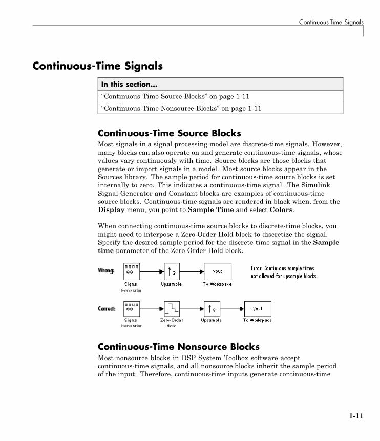
Continuous-Time Signals
In this section...
“Continuous-Time Source Blocks” on page 1-11
“Continuous-Time Nonsource Blocks” on page 1-11
Continuous-Time Source BlocksMost signals in a signal processing model are discrete-time signals. However,many blocks can also operate on and generate continuous-time signals, whosevalues vary continuously with time. Source blocks are those blocks thatgenerate or import signals in a model. Most source blocks appear in theSources library. The sample period for continuous-time source blocks is setinternally to zero. This indicates a continuous-time signal. The SimulinkSignal Generator and Constant blocks are examples of continuous-timesource blocks. Continuous-time signals are rendered in black when, from theDisplay menu, you point to Sample Time and select Colors.
When connecting continuous-time source blocks to discrete-time blocks, youmight need to interpose a Zero-Order Hold block to discretize the signal.Specify the desired sample period for the discrete-time signal in the Sampletime parameter of the Zero-Order Hold block.
Continuous-Time Nonsource BlocksMost nonsource blocks in DSP System Toolbox software acceptcontinuous-time signals, and all nonsource blocks inherit the sample periodof the input. Therefore, continuous-time inputs generate continuous-time
1-11

1 Input, Output, and Display
outputs. Blocks that are not capable of accepting continuous-time signalsinclude the Digital Filter, FIR Decimation, FIR Interpolation blocks.
1-12

Create Sample-Based Signals
Create Sample-Based Signals
Note Starting in R2010b, many DSP System Toolbox blocks received a newparameter to control whether they perform sample- or frame-based processing.The following content has not been updated to reflect this change. For moreinformation, see the “Frame-Based Processing” section of the Release Notes.
In this section...
“Create Signals Using Constant Block” on page 1-13
“Create Signals Using Signal from Workspace Block” on page 1-16
Create Signals Using Constant BlockA constant sample-based signal has identical successive samples. The Sourceslibrary provides the following blocks for creating constant sample-basedsignals:
• Constant Diagonal Matrix
• Constant
• Identity Matrix
The most versatile of the blocks listed above is the Constant block. This topicdiscusses how to create a constant sample-based signal using the Constantblock:
1 Create a new Simulink model.
2 From the Sources library, click-and-drag a Constant block into the model.
3 From the Sinks library, click-and-drag a Display block into the model.
4 Connect the two blocks.
5 Double-click the Constant block, and set the block parameters as follows:
• Constant value = [1 2 3; 4 5 6]
1-13
1 Input, Output, and Display
• Interpret vector parameters as 1–D = Clear this check box
• Sampling Mode = Sample based
• Sample time = 1
Based on these parameters, the Constant block outputs a constant,discrete-valued, sample-based matrix signal with a sample period of 1second.
The Constant block’s Constant value parameter can be any validMATLAB variable or expression that evaluates to a matrix.
6 Save these parameters and close the dialog box by clicking OK.
7 From the Display menu, point to Signals & Ports and select SignalDimensions.
8 Run the model and expand the Display block so you can view the entiresignal.
You have now successfully created a six-channel, constant sample-basedsignal with a sample period of 1 second.
To view the model you just created, and to learn how to create a 1–D vectorsignal from the block diagram you just constructed, continue to the nextsection.
Create an Unoriented Vector SignalYou can create an unoriented vector by modifying the block diagram youconstructed in the previous section:
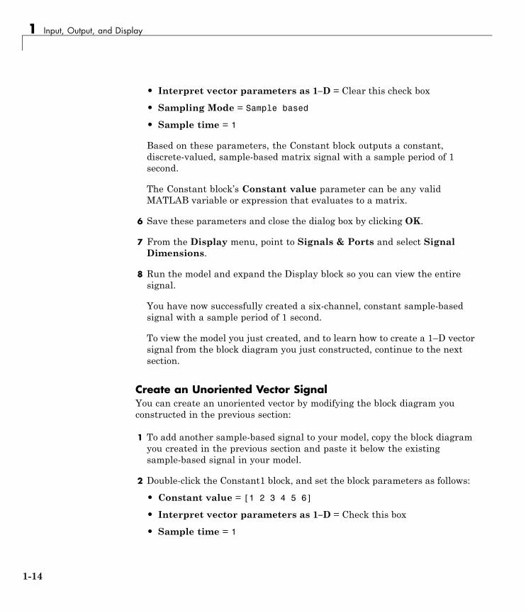
1 To add another sample-based signal to your model, copy the block diagramyou created in the previous section and paste it below the existingsample-based signal in your model.
2 Double-click the Constant1 block, and set the block parameters as follows:
• Constant value = [1 2 3 4 5 6]
• Interpret vector parameters as 1–D = Check this box
• Sample time = 1
1-14
Create Sample-Based Signals
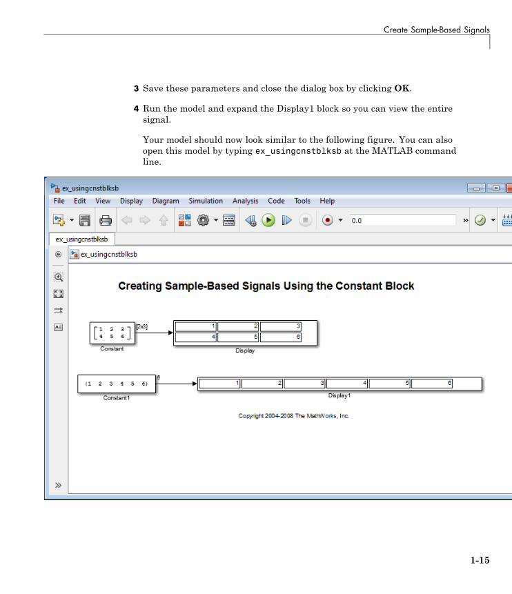
3 Save these parameters and close the dialog box by clicking OK.
4 Run the model and expand the Display1 block so you can view the entiresignal.
Your model should now look similar to the following figure. You can alsoopen this model by typing ex_usingcnstblksb at the MATLAB commandline.
1-15
1 Input, Output, and Display
The Constant1 block generates a length-6 unoriented vector signal. Thismeans that the output is not a matrix. However, most nonsource signalprocessing blocks interpret a length-M unoriented vector as an M-by-1 matrix(column vector).
Create Signals Using Signal from Workspace BlockThis topic discusses how to create a four-channel sample-based signal with asample period of 1 second using the Signal From Workspace block:
1 Create a new Simulink model.
2 From the Sources library, click-and-drag a Signal From Workspace blockinto the model.
3 From the Sinks library, click-and-drag a Signal To Workspace block intothe model.
4 Connect the two blocks.
5 Double-click the Signal From Workspace block, and set the blockparameters as follows:
• Signal = cat(3,[1 -1;0 5],[2 -2;0 5],[3 -3;0 5])
• Sample time = 1
• Samples per frame = 1
• Form output after final data value by = Setting to zero
Based on these parameters, the Signal From Workspace block outputs afour-channel sample-based signal with a sample period of 1 second. Afterthe block has output the signal, all subsequent outputs have a value ofzero. The four channels contain the following values:
• Channel 1: 1, 2, 3, 0, 0,...
• Channel 2: -1, -2, -3, 0, 0,...
• Channel 3: 0, 0, 0, 0, 0,...
• Channel 4: 5, 5, 5, 0, 0,...
6 Save these parameters and close the dialog box by clicking OK.
1-16

Create Sample-Based Signals
7 From the Display menu, point to Signals & Ports, and select SignalDimensions.
8 Run the model.
The following figure is a graphical representation of the model’sbehavior during simulation. You can also open the model by typingex_usingsfwblksb at the MATLAB command line.
9 At the MATLAB command line, type yout.
The following is a portion of the output:
yout(:,:,1) =
1 -10 5
yout(:,:,2) =
2 -20 5
yout(:,:,3) =
3 -30 5
1-17

1 Input, Output, and Display
yout(:,:,4) =
0 00 0
You have now successfully created a four-channel sample-based signal withsample period of 1 second using the Signal From Workspace block.
1-18
Create Frame-Based Signals
Create Frame-Based Signals
Note Starting in R2010b, many DSP System Toolbox blocks received a newparameter to control whether they perform sample- or frame-based processing.The following content has not been updated to reflect this change. For moreinformation, see the “Frame-Based Processing” section of the Release Notes.
In this section...
“Create Signals Using Sine Wave Block” on page 1-19
“Create Signals Using Signal from Workspace Block” on page 1-22
Create Signals Using Sine Wave BlockA frame-based signal is propagated through a model in batches of samplescalled frames. Frame-based processing can significantly improve theperformance of your model by decreasing the amount of time it takes yoursimulation to run.
One of the most commonly used blocks in the Sources library is the Sine Waveblock. This topic describes how to create a three-channel frame-based signalusing the Sine Wave block:
1 Create a new Simulink model.
2 From the Sources library, click-and-drag a Sine Wave block into the model.
3 From the Matrix Operations library, click-and-drag a Matrix Sum blockinto the model.
4 From the Sinks library, click-and-drag a Signal to Workspace block intothe model.
5 Connect the blocks in the order in which you added them to your model.
6 Double-click the Sine Wave block, and set the block parameters as follows:
• Amplitude = [1 3 2]
1-19

1 Input, Output, and Display
• Frequency = [100 250 500]
• Sample time = 1/5000
• Samples per frame = 64
Based on these parameters, the Sine Wave block outputs three sinusoidswith amplitudes 1, 3, and 2 and frequencies 100, 250, and 500 hertz,respectively. The sample period, 1/5000, is 10 times the highest sinusoidfrequency, which satisfies the Nyquist criterion. The frame size is 64 for allsinusoids, and, therefore, the output has 64 rows.
7 Save these parameters and close the dialog box by clicking OK.
You have now successfully created a three-channel frame-based signalusing the Sine Wave block. The rest of this procedure describes how toadd these three sinusoids together.
8 Double-click the Matrix Sum block. Set the Sum over parameter toSpecified dimension, and set the Dimension parameter to 2. Click OK.
9 From the Display menu, point to Signals & Ports, and select SignalDimensions.
10 Run the model.
Your model should now look similar to the following figure. You canalso open the model by typing ex_usingsinwaveblkfb at the MATLABcommand line.
1-20
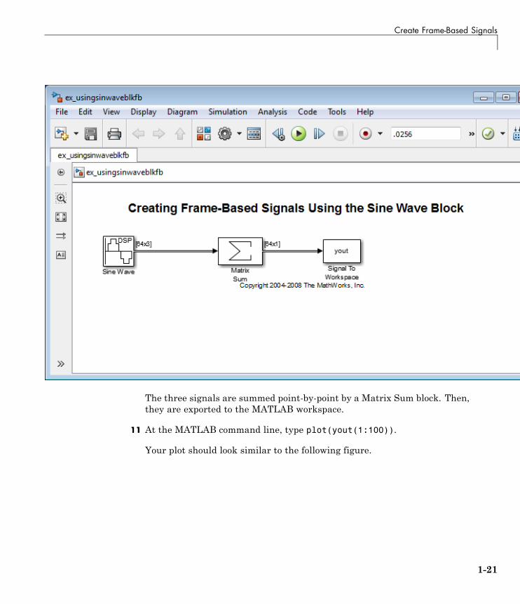
Create Frame-Based Signals
The three signals are summed point-by-point by a Matrix Sum block. Then,they are exported to the MATLAB workspace.
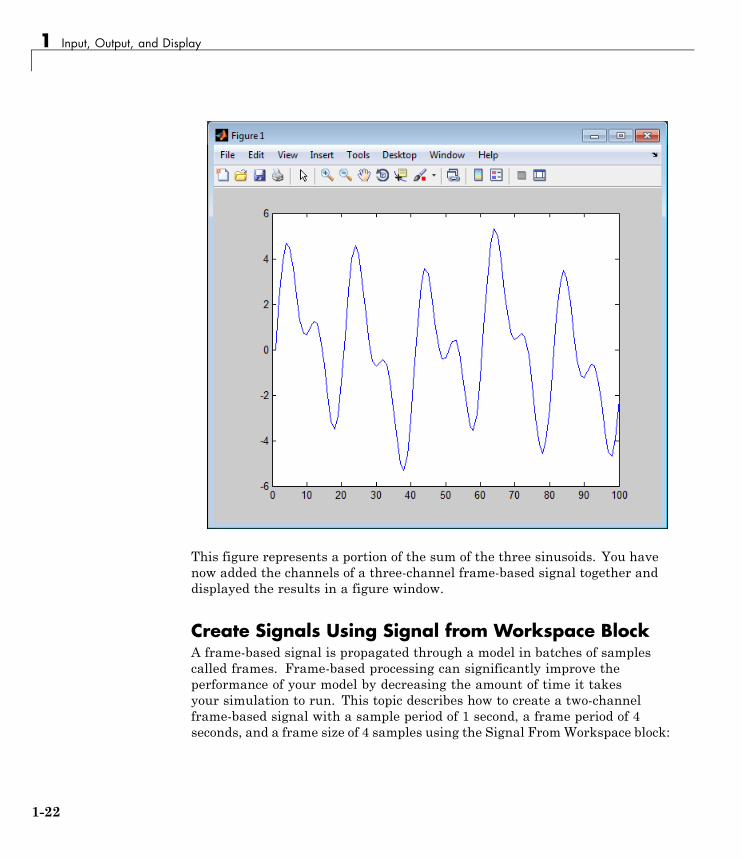
11 At the MATLAB command line, type plot(yout(1:100)).
Your plot should look similar to the following figure.
1-21
1 Input, Output, and Display
This figure represents a portion of the sum of the three sinusoids. You havenow added the channels of a three-channel frame-based signal together anddisplayed the results in a figure window.
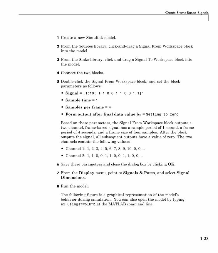
Create Signals Using Signal from Workspace BlockA frame-based signal is propagated through a model in batches of samplescalled frames. Frame-based processing can significantly improve theperformance of your model by decreasing the amount of time it takesyour simulation to run. This topic describes how to create a two-channelframe-based signal with a sample period of 1 second, a frame period of 4seconds, and a frame size of 4 samples using the Signal FromWorkspace block:
1-22
Create Frame-Based Signals
1 Create a new Simulink model.
2 From the Sources library, click-and-drag a Signal From Workspace blockinto the model.
3 From the Sinks library, click-and-drag a Signal To Workspace block intothe model.
4 Connect the two blocks.
5 Double-click the Signal From Workspace block, and set the blockparameters as follows:
• Signal = [1:10; 1 1 0 0 1 1 0 0 1 1]'
• Sample time = 1
• Samples per frame = 4
• Form output after final data value by = Setting to zero
Based on these parameters, the Signal From Workspace block outputs atwo-channel, frame-based signal has a sample period of 1 second, a frameperiod of 4 seconds, and a frame size of four samples. After the blockoutputs the signal, all subsequent outputs have a value of zero. The twochannels contain the following values:
• Channel 1: 1, 2, 3, 4, 5, 6, 7, 8, 9, 10, 0, 0,...
• Channel 2: 1, 1, 0, 0, 1, 1, 0, 0, 1, 1, 0, 0,...
6 Save these parameters and close the dialog box by clicking OK.
7 From the Display menu, point to Signals & Ports, and select SignalDimensions.
8 Run the model.
The following figure is a graphical representation of the model’sbehavior during simulation. You can also open the model by typingex_usingsfwblkfb at the MATLAB command line.
1-23
1 Input, Output, and Display
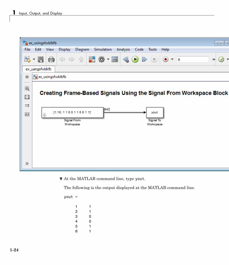
9 At the MATLAB command line, type yout.
The following is the output displayed at the MATLAB command line.
yout =
1 12 13 04 05 16 1
1-24

Create Frame-Based Signals
7 08 09 1
10 10 00 0
Note that zeros were appended to the end of each channel. You have nowsuccessfully created a two-channel frame-based signal and exported it to theMATLAB workspace.
1-25
1 Input, Output, and Display
Create Multichannel Sample-Based Signals
In this section...
“Multichannel Sample-Based Signals” on page 1-26
“Create Multichannel Signals by Combining Single-Channel Signals” onpage 1-26
“Create Multichannel Signals by Combining Multichannel Signals” on page1-29
Multichannel Sample-Based SignalsWhen you want to perform the same operations on several independentsignals, you can group those signals together as a multichannel signal. Forexample, if you need to filter each of four independent signals using thesame direct-form II transpose filter, you can combine the signals into amultichannel signal, and connect the signal to a single Digital Filter Designblock. The block applies the filter to each channel independently.
A sample-based signal with M*N channels is represented by a sequence ofM-by-N matrices. Multiple sample-based signals can be combined into asingle multichannel sample-based signal using the Concatenate block. Inaddition, several multichannel sample-based signals can be combined into asingle multichannel sample-based signal using the same technique.
Create Multichannel Signals by CombiningSingle-Channel SignalsYou can combine individual sample-based signals into a multichannel signalby using the Matrix Concatenate block in the Simulink Math Operationslibrary:
1 Open the Matrix Concatenate Example 1 model by typing
ex_cmbsnglchsbsigs
at the MATLAB command line.
1-26

Create Multichannel Sample-Based Signals
1-27

1 Input, Output, and Display
2 Double-click the Signal From Workspace block, and set the Signalparameter to 1:10. Click OK.
3 Double-click the Signal From Workspace1 block, and set the Signalparameter to -1:-1:-10. Click OK.
4 Double-click the Signal From Workspace2 block, and set the Signalparameter to zeros(10,1). Click OK.
5 Double-click the Signal From Workspace3 block, and set the Signalparameter to 5*ones(10,1). Click OK.
6 Double-click the Matrix Concatenate block. Set the block parameters asfollows, and then click OK:
• Number of inputs = 4
• Mode = Multidimensional array
• Concatenate dimension = 1
7 Double-click the Reshape block. Set the block parameters as follows, andthen click OK:
• Output dimensionality = Customize
• Output dimensions = [2,2]
8 Run the model.
Four independent sample-based signals are combined into a 2-by-2multichannel matrix signal.
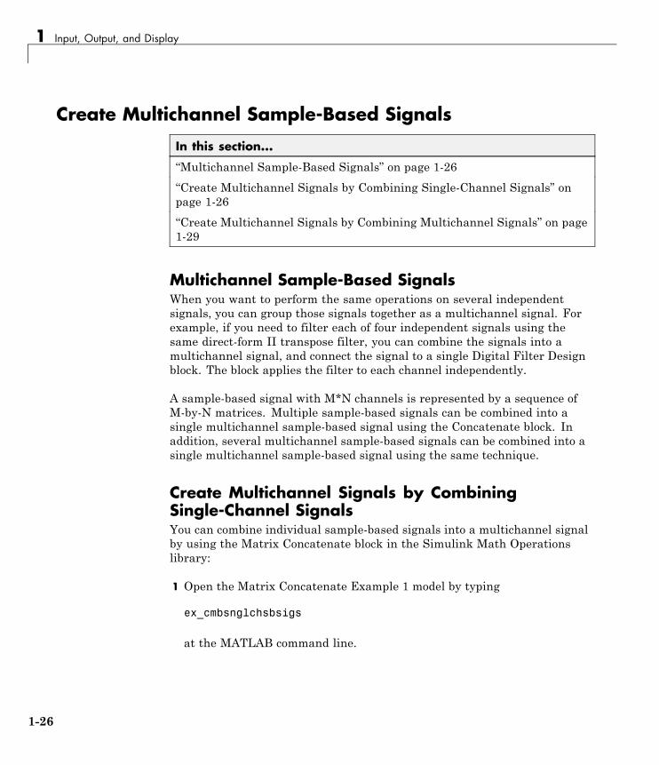
Each 4-by-1 output from the Matrix Concatenate block contains one samplefrom each of the four input signals at the same instant in time. TheReshape block rearranges the samples into a 2-by-2 matrix. Each elementof this matrix is a separate channel.
Note that the Reshape block works columnwise, so that a column vectorinput is reshaped as shown below.
1-28
Create Multichannel Sample-Based Signals
The 4-by-1 matrix output by the Matrix Concatenate block and the 2-by-2matrix output by the Reshape block in the above model represent the samefour-channel sample-based signal. In some cases, one representation of thesignal may be more useful than the other.
9 At the MATLAB command line, type dsp_examples_yout.
The four-channel, sample-based signal is displayed as a series of matricesin the MATLAB Command Window. Note that the last matrix containsonly zeros. This is because every Signal From Workspace block in thismodel has its Form output after final data value by parameter setto Setting to Zero.
Create Multichannel Signals by CombiningMultichannel SignalsYou can combine existing multichannel sample-based signals into largermultichannel signals using the Simulink Matrix Concatenate block:
1 Open the Matrix Concatenate Example 2 model by typing
ex_cmbmltichsbsigs
at the MATLAB command line.
1-29

1 Input, Output, and Display
1-30

Create Multichannel Sample-Based Signals
2 Double-click the Signal From Workspace block, and set the Signalparameter to [1:10;-1:-1:-10]'. Click OK.
3 Double-click the Signal From Workspace1 block, and set the Signalparameter to [zeros(10,1) 5*ones(10,1)]. Click OK.
4 Double-click the Matrix Concatenate block. Set the block parameters asfollows, and then click OK:
• Number of inputs = 2
• Mode = Multidimensional array
• Concatenate dimension = 1
5 Run the model.
The model combines both two-channel sample-based signals into afour-channel signal.
Each 2-by-2 output from the Matrix Concatenate block contains bothsamples from each of the two input signals at the same instant in time.Each element of this matrix is a separate channel.
1-31
1 Input, Output, and Display
Create Multichannel Frame-Based Signals
In this section...
“Multichannel Frame-Based Signals” on page 1-32
“Create Multichannel Signals Using Concatenate Block” on page 1-33
Multichannel Frame-Based SignalsWhen you want to perform the same operations on several independentsignals, you can group those signals together as a multichannel signal. Forexample, if you need to filter each of four independent signals using thesame direct-form II transpose filter, you can combine the signals into amultichannel signal, and connect the signal to a single Digital Filter Designblock. The block applies the filter to each channel independently.
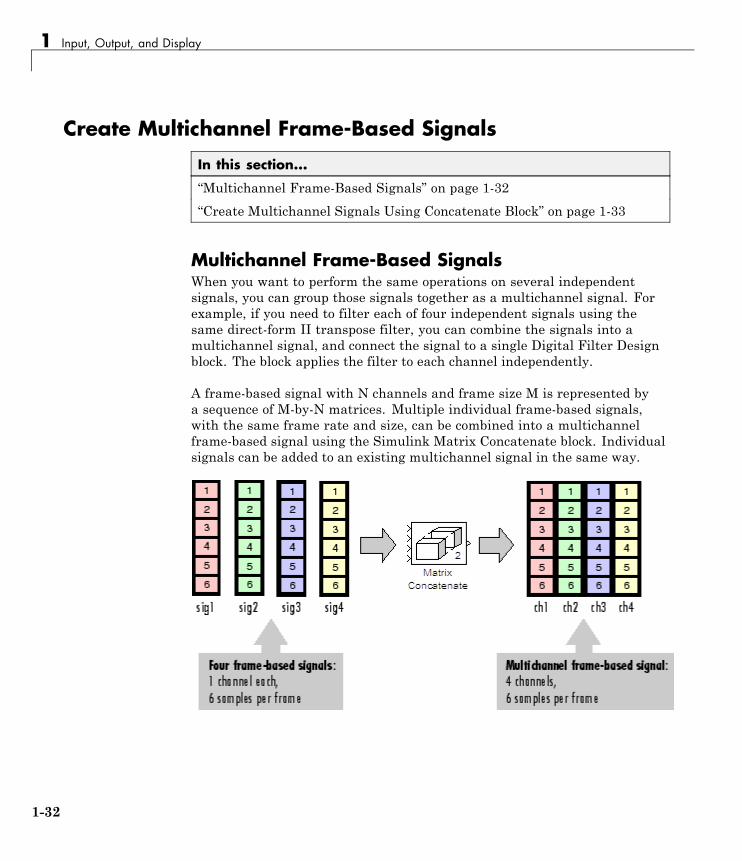
A frame-based signal with N channels and frame size M is represented bya sequence of M-by-N matrices. Multiple individual frame-based signals,with the same frame rate and size, can be combined into a multichannelframe-based signal using the Simulink Matrix Concatenate block. Individualsignals can be added to an existing multichannel signal in the same way.
1-32
Create Multichannel Frame-Based Signals
Create Multichannel Signals Using Concatenate BlockYou can combine existing frame-based signals into a larger multichannelsignal by using the Simulink Concatenate block. All signals must havethe same frame rate and frame size. In this example, a single-channelframe-based signal is combined with a two-channel frame-based signal toproduce a three-channel frame-based signal:
1 Open the Matrix Concatenate Example 3 model by typing
ex_combiningfbsigs
at the MATLAB command line.
1-33

1 Input, Output, and Display
1-34

Create Multichannel Frame-Based Signals
2 Double-click the Signal From Workspace block. Set the block parametersas follows:
• Signal = [1:10;-1:-1:-10]'
• Sample time = 1
• Samples per frame = 4
Based on these parameters, the Signal From Workspace block outputs aframe-based signal with a frame size of four.
3 Save these parameters and close the dialog box by clicking OK.
4 Double-click the Signal From Workspace1 block. Set the block parametersas follows, and then click OK:
• Signal = 5*ones(10,1)
• Sample time = 1
• Samples per frame = 4
The Signal From Workspace1 block has the same sample time and framesize as the Signal From Workspace block. When you combine frame-basedsignals into multichannel signals, the original signals must have the sameframe rate and frame size.
5 Double-click the Matrix Concatenate block. Set the block parameters asfollows, and then click OK:
• Number of inputs = 2
• Mode = Multidimensional array
• Concatenate dimension = 2
6 Run the model.
The 4-by-3 matrix output from the Matrix Concatenate block contains allthree input channels, and preserves their common frame rate and framesize.
1-35

1 Input, Output, and Display
Deconstruct Multichannel Sample-Based Signals
Note Starting in R2010b, many DSP System Toolbox blocks received a newparameter to control whether they perform sample- or frame-based processing.The following content has not been updated to reflect this change. For moreinformation, see the “Frame-Based Processing” section of the Release Notes.
In this section...
“Split Multichannel Signals into Individual Signals” on page 1-36
“Split Multichannel Signals into Several Multichannel Signals” on page 1-39
Split Multichannel Signals into Individual SignalsMultichannel signals, represented by matrices in the Simulink environment,are frequently used in signal processing models for efficiency and compactness.Though most of the signal processing blocks can process multichannel signals,you may need to access just one channel or a particular range of samples in amultichannel signal. You can access individual channels of the multichannelsignal by using the blocks in the Indexing library. This library includes theSelector, Submatrix, Variable Selector, Multiport Selector, and Submatrixblocks.
You can split a multichannel sample-based signal into single-channelsample-based signals using the Multiport Selector block. This block allowsyou to select specific rows and/or columns and propagate the selection to achosen output port. In this example, a three-channel sample-based signal isdeconstructed into three independent sample-based signals:
1 Open the Multiport Selector Example 1 model by typingex_splitmltichsbsigsind at the MATLAB command line.
1-36

Deconstruct Multichannel Sample-Based Signals
2 Double-click the Signal From Workspace block, and set the blockparameters as follows:
1-37
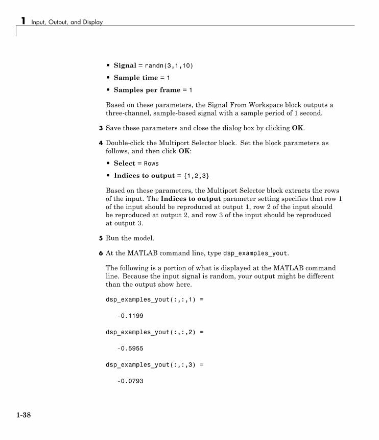
1 Input, Output, and Display
• Signal = randn(3,1,10)
• Sample time = 1
• Samples per frame = 1
Based on these parameters, the Signal From Workspace block outputs athree-channel, sample-based signal with a sample period of 1 second.
3 Save these parameters and close the dialog box by clicking OK.
4 Double-click the Multiport Selector block. Set the block parameters asfollows, and then click OK:
• Select = Rows
• Indices to output = {1,2,3}
Based on these parameters, the Multiport Selector block extracts the rowsof the input. The Indices to output parameter setting specifies that row 1of the input should be reproduced at output 1, row 2 of the input shouldbe reproduced at output 2, and row 3 of the input should be reproducedat output 3.
5 Run the model.
6 At the MATLAB command line, type dsp_examples_yout.
The following is a portion of what is displayed at the MATLAB commandline. Because the input signal is random, your output might be differentthan the output show here.
dsp_examples_yout(:,:,1) =
-0.1199
dsp_examples_yout(:,:,2) =
-0.5955
dsp_examples_yout(:,:,3) =
-0.0793
1-38

Deconstruct Multichannel Sample-Based Signals
This sample-based signal is the first row of the input to the MultiportSelector block. You can view the other two input rows by typingdsp_examples_yout1 and dsp_examples_yout2, respectively.
You have now successfully created three, single-channel sample-based signalsfrom a multichannel sample-based signal using a Multiport Selector block.
Split Multichannel Signals into Several MultichannelSignalsMultichannel signals, represented by matrices in the Simulink environment,are frequently used in signal processing models for efficiency and compactness.Though most of the signal processing blocks can process multichannel signals,you may need to access just one channel or a particular range of samples in amultichannel signal. You can access individual channels of the multichannelsignal by using the blocks in the Indexing library. This library includes theSelector, Submatrix, Variable Selector, Multiport Selector, and Submatrixblocks.
You can split a multichannel sample-based signal into other multichannelsample-based signals using the Submatrix block. The Submatrix block is themost versatile of the blocks in the Indexing library because it allows arbitrarychannel selections. Therefore, you can extract a portion of a multichannelsample-based signal. In this example, you extract a six-channel, sample-basedsignal from a 35-channel, sample-based signal (5-by-7 matrix):
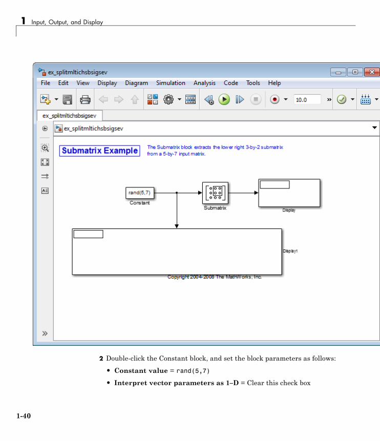
1 Open the Submatrix Example model by typing ex_splitmltichsbsigsevat the MATLAB command line.
1-39
1 Input, Output, and Display
2 Double-click the Constant block, and set the block parameters as follows:
• Constant value = rand(5,7)
• Interpret vector parameters as 1–D = Clear this check box
1-40

Deconstruct Multichannel Sample-Based Signals
• Sampling mode = Sample based
• Sample Time = 1
Based on these parameters, the Constant block outputs a constant-valued,sample-based signal.
3 Save these parameters and close the dialog box by clicking OK.
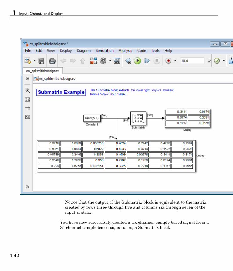
4 Double-click the Submatrix block. Set the block parameters as follows,and then click OK:
• Row span = Range of rows
• Starting row = Index
• Starting row index = 3
• Ending row = Last
• Column span = Range of columns
• Starting column = Offset from last
• Starting column offset = 1
• Ending column = Last
Based on these parameters, the Submatrix block outputs rows three to five,the last row of the input signal. It also outputs the second to last columnand the last column of the input signal.
5 Run the model.
The model should now look similar to the following figure.
1-41
1 Input, Output, and Display
Notice that the output of the Submatrix block is equivalent to the matrixcreated by rows three through five and columns six through seven of theinput matrix.
You have now successfully created a six-channel, sample-based signal from a35-channel sample-based signal using a Submatrix block.
1-42

Deconstruct Multichannel Frame-Based Signals
Deconstruct Multichannel Frame-Based Signals
Note Starting in R2010b, many DSP System Toolbox blocks received a newparameter to control whether they perform sample- or frame-based processing.The following content has not been updated to reflect this change. For moreinformation, see the “Frame-Based Processing” section of the Release Notes.
In this section...
“Split Multichannel Signals into Individual Signals” on page 1-43
“Reorder Channels in Multichannel Frame-Based Signals” on page 1-48
Split Multichannel Signals into Individual SignalsMultichannel signals, represented by matrices in the Simulink environment,are frequently used in signal processing models for efficiency and compactness.Though most of the signal processing blocks can process multichannel signals,you may need to access just one channel or a particular range of samples in amultichannel signal. You can access individual channels of the multichannelsignal by using the blocks in the Indexing library. This library includes theSelector, Submatrix, Variable Selector, Multiport Selector, and Submatrixblocks. It is also possible to use the Permute Matrix block, in the Matrixoperations library, to reorder the channels of a frame-based signal.
You can use the Multiport Selector block in the Indexing library to extract theindividual channels of a multichannel frame-based signal. These signals formsingle-channel frame-based signals that have the same frame rate and sizeof the multichannel signal.
The figure below is a graphical representation of this process.
1-43
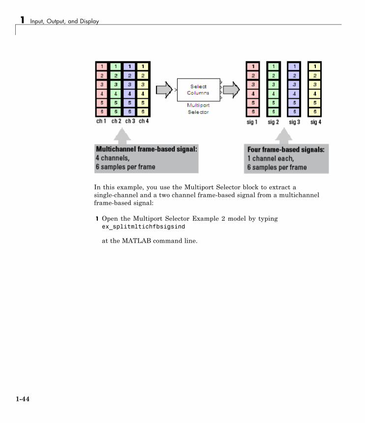
1 Input, Output, and Display
In this example, you use the Multiport Selector block to extract asingle-channel and a two channel frame-based signal from a multichannelframe-based signal:
1 Open the Multiport Selector Example 2 model by typingex_splitmltichfbsigsind
at the MATLAB command line.
1-44

Deconstruct Multichannel Frame-Based Signals
1-45

1 Input, Output, and Display
2 Double-click the Signal From Workspace block, and set the blockparameters as follows:
• Signal = [1:10;-1:-1:-10;5*ones(1,10)]'
• Samples per frame = 4
Based on these parameters, the Signal From Workspace block outputs athree-channel, frame-based signal with a frame size of four.
3 Save these parameters and close the dialog box by clicking OK.
4 Double-click the Multiport Selector block. Set the block parameters asfollows, and then click OK:
• Select = Columns
• Indices to output = {[1 3],2}
Based on these parameters, the Multiport Selector block outputs the firstand third columns at the first output port and the second column at thesecond output port of the block. Setting the Select parameter to Columnsensures that the block preserves the frame rate and frame size of the input.
5 Run the model.
The figure below is a graphical representation of how the MultiportSelector block splits one frame of the three-channel frame-based signal intoa single-channel signal and a two-channel signal.
1-46

Deconstruct Multichannel Frame-Based Signals
The Multiport Selector block outputs a two-channel frame-based signal,comprised of the first and third column of the input signal, at the first port. Itoutputs a single-channel frame-based signal, comprised of the second columnof the input signal, at the second port.
You have now successfully created a single-channel and a two-channelframe-based signal from a multichannel frame-based signal using theMultiport Selector block.
1-47
1 Input, Output, and Display
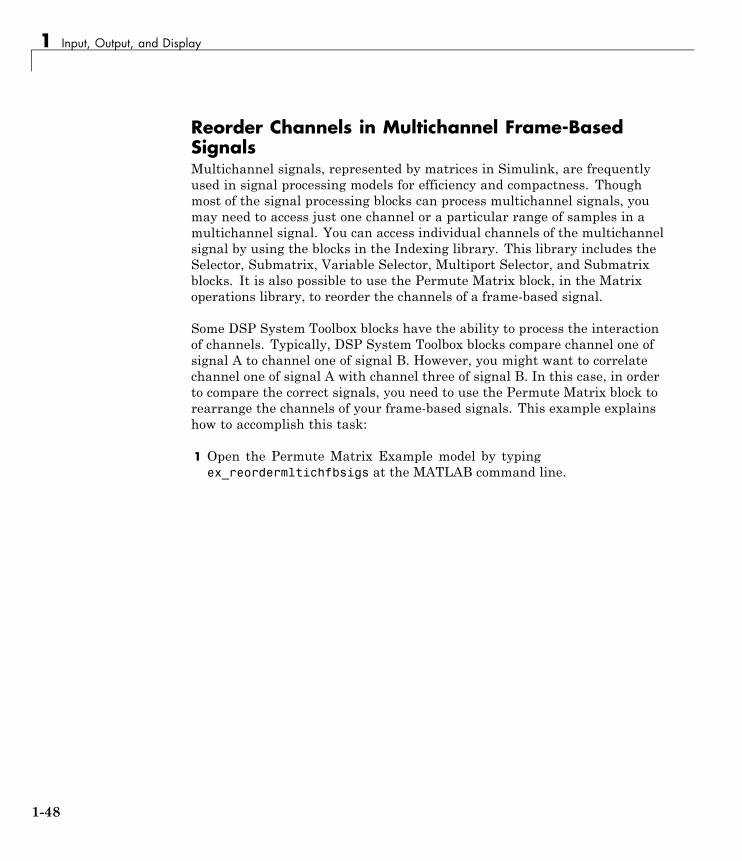
Reorder Channels in Multichannel Frame-BasedSignalsMultichannel signals, represented by matrices in Simulink, are frequentlyused in signal processing models for efficiency and compactness. Thoughmost of the signal processing blocks can process multichannel signals, youmay need to access just one channel or a particular range of samples in amultichannel signal. You can access individual channels of the multichannelsignal by using the blocks in the Indexing library. This library includes theSelector, Submatrix, Variable Selector, Multiport Selector, and Submatrixblocks. It is also possible to use the Permute Matrix block, in the Matrixoperations library, to reorder the channels of a frame-based signal.
Some DSP System Toolbox blocks have the ability to process the interactionof channels. Typically, DSP System Toolbox blocks compare channel one ofsignal A to channel one of signal B. However, you might want to correlatechannel one of signal A with channel three of signal B. In this case, in orderto compare the correct signals, you need to use the Permute Matrix block torearrange the channels of your frame-based signals. This example explainshow to accomplish this task:
1 Open the Permute Matrix Example model by typingex_reordermltichfbsigs at the MATLAB command line.
1-48

Deconstruct Multichannel Frame-Based Signals
2 Double-click the Signal From Workspace block, and set the blockparameters as follows:
• Signal = [1:10;-1:-1:-10;5*ones(1,10)]'
1-49

1 Input, Output, and Display
• Sample time = 1
• Samples per frame = 4
Based on these parameters, the Signal From Workspace block outputs athree-channel, frame-based signal with a sample period of 1 second and aframe size of 4. The frame period of this block is 4 seconds.
3 Save these parameters and close the dialog box by clicking OK.
4 Double-click the Constant block. Set the block parameters as follows, andthen click OK:
• Constant value = [1 3 2]
• Interpret vector parameters as 1–D = Clear this check box
• Sampling mode = Frame based
• Frame period = 4
The discrete-time, frame-based vector output by the Constant block tellsthe Permute Matrix block to swap the second and third columns of theinput signal. Note that the frame period of the Constant block must matchthe frame period of the Signal From Workspace block.
5 Double-click the Permute Matrix block. Set the block parameters asfollows, and then click OK:
• Permute = Columns
• Index mode = One-based
Based on these parameters, the Permute Matrix block rearranges thecolumns of the input signal, and the index of the first column is now one.
6 Run the model.
The figure below is a graphical representation of what happens to the firstinput frame during simulation.
1-50
Deconstruct Multichannel Frame-Based Signals
The second and third channel of the frame-based input signal are swapped.
7 At the MATLAB command line, type yout.
You can now verify that the second and third columns of the input signalare rearranged.
You have now successfully reordered the channels of a frame-based signalusing the Permute Matrix block.
1-51

1 Input, Output, and Display
Import and Export Sample-Based Signals
Note Starting in R2010b, many DSP System Toolbox blocks received a newparameter to control whether they perform sample- or frame-based processing.The following content has not been updated to reflect this change. For moreinformation, see the “Frame-Based Processing” section of the Release Notes.
In this section...
“Import Sample-Based Vector Signals” on page 1-52
“Import Sample-Based Matrix Signals” on page 1-56
“Export Sample-Based Signals” on page 1-59
Import Sample-Based Vector SignalsThe Signal From Workspace block generates a sample-based vector signalwhen the variable or expression in the Signal parameter is a matrix and theSamples per frame parameter is set to 1. Each column of the input matrixrepresents a different channel. Beginning with the first row of the matrix, theblock outputs one row of the matrix at each sample time. Therefore, if theSignal parameter specifies an M-by-N matrix, the output of the Signal FromWorkspace block is M 1-by-N row vectors representing N channels.
The figure below is a graphical representation of this process for a 6-by-4workspace matrix, A.
1-52

Import and Export Sample-Based Signals
In the following example, you use the Signal From Workspace block to importa sample-based vector signal into your model:
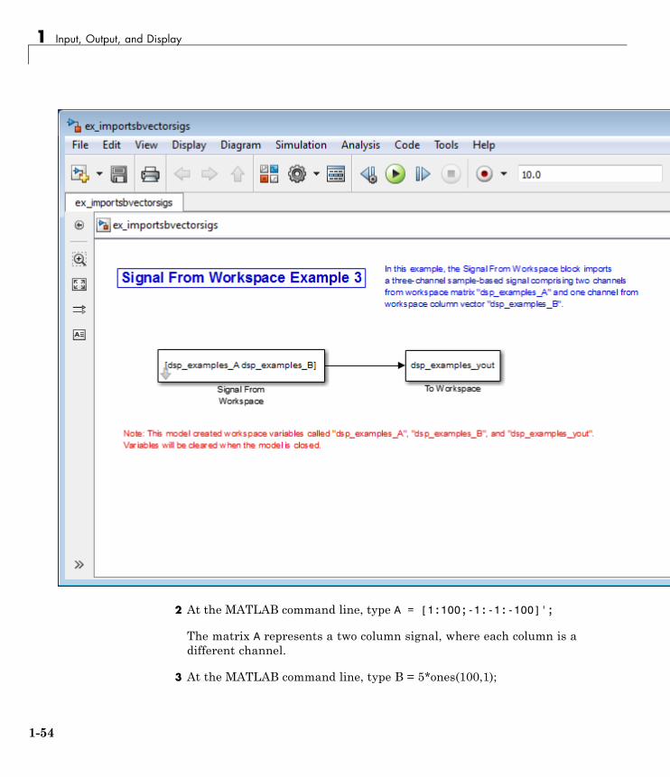
1 Open the Signal From Workspace Example 3 model by typingex_importsbvectorsigs at the MATLAB command line.
1-53
1 Input, Output, and Display
2 At the MATLAB command line, type A = [1:100;-1:-1:-100]';
The matrix A represents a two column signal, where each column is adifferent channel.
3 At the MATLAB command line, type B = 5*ones(100,1);
1-54
Import and Export Sample-Based Signals
The vector B represents a single-channel signal.
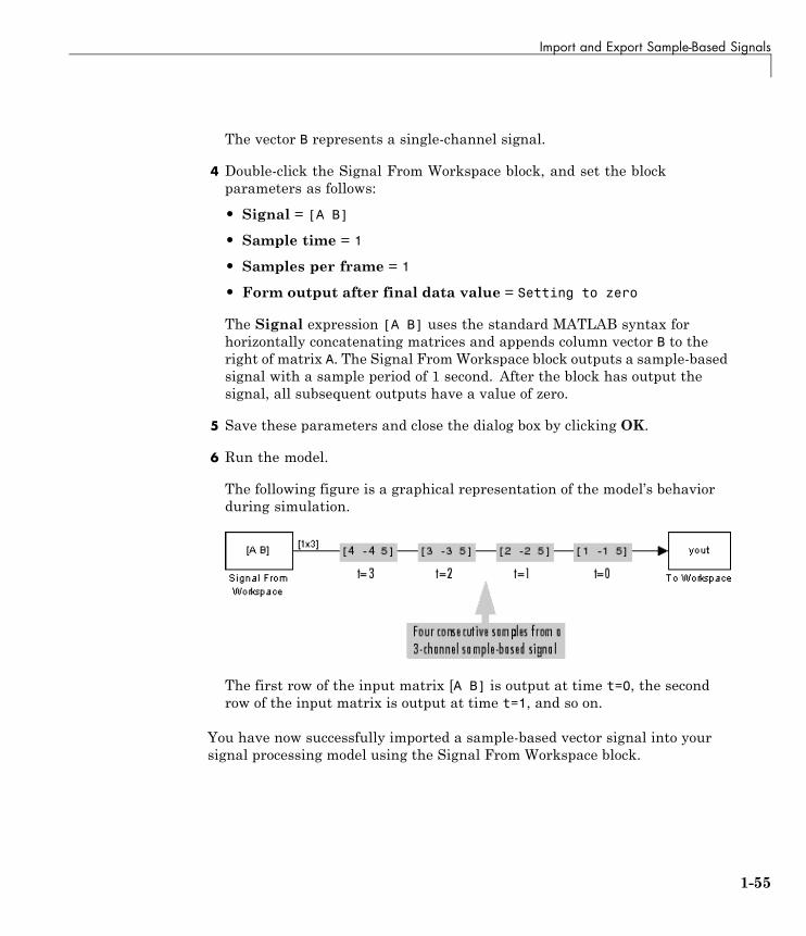
4 Double-click the Signal From Workspace block, and set the blockparameters as follows:
• Signal = [A B]
• Sample time = 1
• Samples per frame = 1
• Form output after final data value = Setting to zero
The Signal expression [A B] uses the standard MATLAB syntax forhorizontally concatenating matrices and appends column vector B to theright of matrix A. The Signal FromWorkspace block outputs a sample-basedsignal with a sample period of 1 second. After the block has output thesignal, all subsequent outputs have a value of zero.
5 Save these parameters and close the dialog box by clicking OK.
6 Run the model.
The following figure is a graphical representation of the model’s behaviorduring simulation.
The first row of the input matrix [A B] is output at time t=0, the secondrow of the input matrix is output at time t=1, and so on.
You have now successfully imported a sample-based vector signal into yoursignal processing model using the Signal From Workspace block.
1-55

1 Input, Output, and Display
Import Sample-Based Matrix SignalsThe Signal From Workspace block generates a sample-based matrixsignal when the variable or expression in the Signal parameter is athree-dimensional array and the Samples per frame parameter is set to 1.Beginning with the first page of the array, the block outputs a single pageof the array to the output at each sample time. Therefore, if the Signalparameter specifies an M-by-N-by-P array, the output of the Signal FromWorkspace block is P M-by-N matrices representing M*N channels.
The following figure is a graphical illustration of this process for a 6-by-4-by-5workspace array A.
In the following example, you use the Signal From Workspace block to importa four-channel, sample-based matrix signal into a Simulink model:
1 Open the Signal From Workspace Example 4 model by typingex_importsbmatrixsigs at the MATLAB command line.
1-56
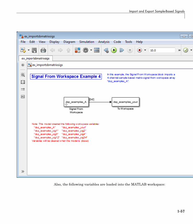
Import and Export Sample-Based Signals
Also, the following variables are loaded into the MATLAB workspace:
1-57
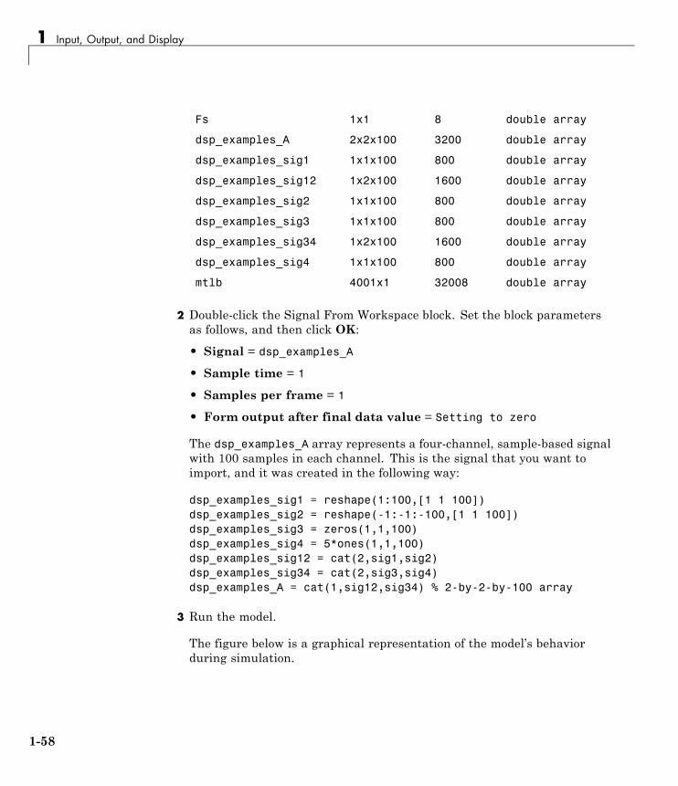
1 Input, Output, and Display
Fs 1x1 8 double array
dsp_examples_A 2x2x100 3200 double array
dsp_examples_sig1 1x1x100 800 double array
dsp_examples_sig12 1x2x100 1600 double array
dsp_examples_sig2 1x1x100 800 double array
dsp_examples_sig3 1x1x100 800 double array
dsp_examples_sig34 1x2x100 1600 double array
dsp_examples_sig4 1x1x100 800 double array
mtlb 4001x1 32008 double array
2 Double-click the Signal From Workspace block. Set the block parametersas follows, and then click OK:
• Signal = dsp_examples_A
• Sample time = 1
• Samples per frame = 1
• Form output after final data value = Setting to zero
The dsp_examples_A array represents a four-channel, sample-based signalwith 100 samples in each channel. This is the signal that you want toimport, and it was created in the following way:
dsp_examples_sig1 = reshape(1:100,[1 1 100])dsp_examples_sig2 = reshape(-1:-1:-100,[1 1 100])dsp_examples_sig3 = zeros(1,1,100)dsp_examples_sig4 = 5*ones(1,1,100)dsp_examples_sig12 = cat(2,sig1,sig2)dsp_examples_sig34 = cat(2,sig3,sig4)dsp_examples_A = cat(1,sig12,sig34) % 2-by-2-by-100 array
3 Run the model.
The figure below is a graphical representation of the model’s behaviorduring simulation.
1-58

Import and Export Sample-Based Signals
The Signal From Workspace block imports the four-channel sample basedsignal from the MATLAB workspace into the Simulink model one matrix ata time.
You have now successfully imported a sample-based matrix signal into yourmodel using the Signal From Workspace block.
Export Sample-Based SignalsThe Signal To Workspace and Triggered To Workspace blocks are the primaryblocks for exporting signals of all dimensions from a Simulink model to theMATLAB workspace.
A sample-based signal, with M*N channels, is represented in Simulink as asequence of M-by-N matrices. When the input to the Signal To Workspaceblock is a sample-based signal, the block creates an M-by-N-by-P array inthe MATLAB workspace containing the P most recent samples from eachchannel. The number of pages, P, is specified by the Limit data points tolast parameter. The newest samples are added at the end of the array.
1-59
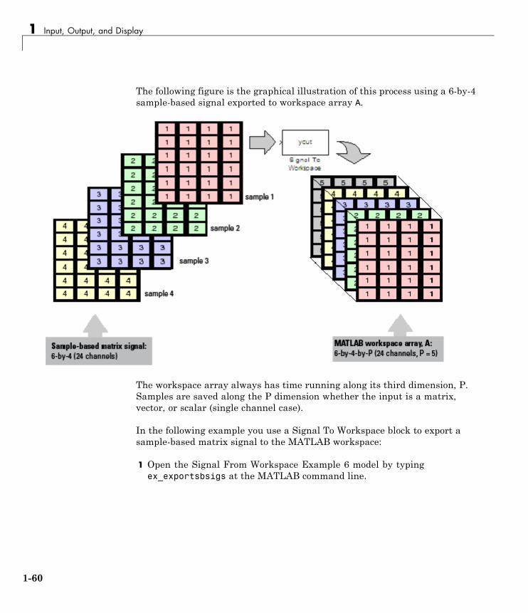
1 Input, Output, and Display
The following figure is the graphical illustration of this process using a 6-by-4sample-based signal exported to workspace array A.
The workspace array always has time running along its third dimension, P.Samples are saved along the P dimension whether the input is a matrix,vector, or scalar (single channel case).
In the following example you use a Signal To Workspace block to export asample-based matrix signal to the MATLAB workspace:
1 Open the Signal From Workspace Example 6 model by typingex_exportsbsigs at the MATLAB command line.
1-60
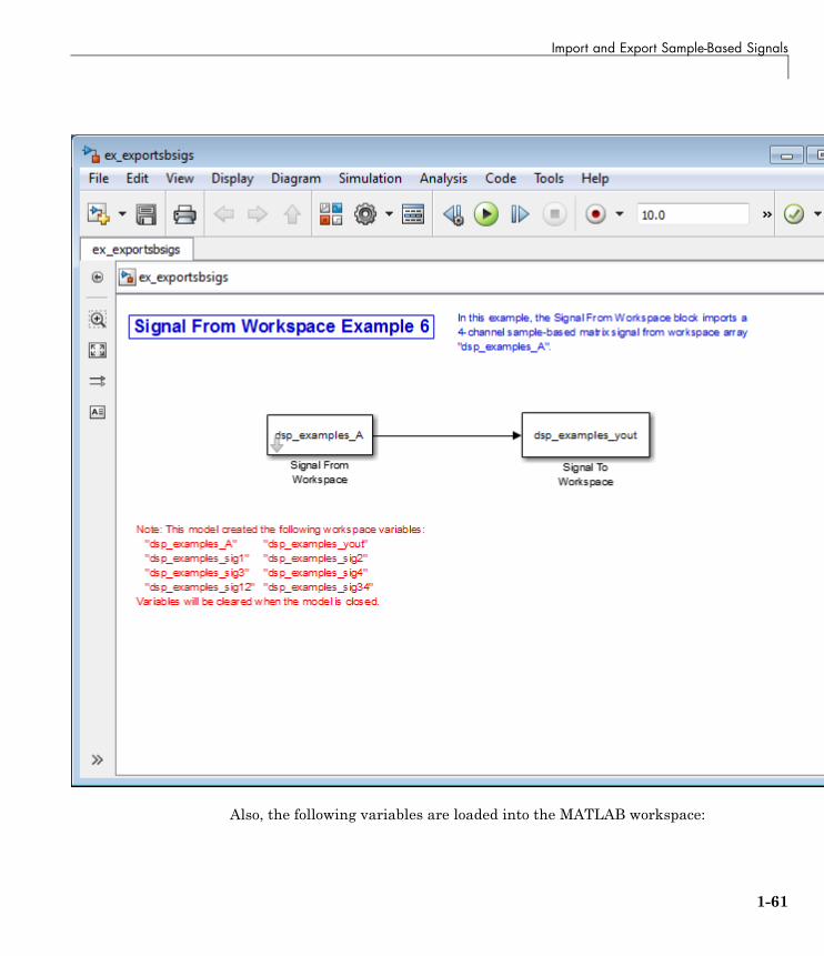
Import and Export Sample-Based Signals
Also, the following variables are loaded into the MATLAB workspace:
1-61
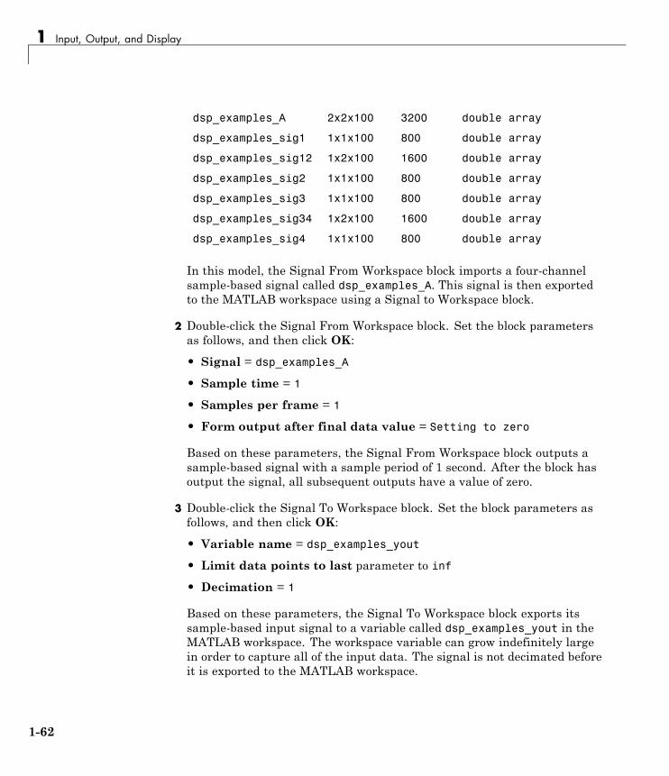
1 Input, Output, and Display
dsp_examples_A 2x2x100 3200 double array
dsp_examples_sig1 1x1x100 800 double array
dsp_examples_sig12 1x2x100 1600 double array
dsp_examples_sig2 1x1x100 800 double array
dsp_examples_sig3 1x1x100 800 double array
dsp_examples_sig34 1x2x100 1600 double array
dsp_examples_sig4 1x1x100 800 double array
In this model, the Signal From Workspace block imports a four-channelsample-based signal called dsp_examples_A. This signal is then exportedto the MATLAB workspace using a Signal to Workspace block.
2 Double-click the Signal From Workspace block. Set the block parametersas follows, and then click OK:
• Signal = dsp_examples_A
• Sample time = 1
• Samples per frame = 1
• Form output after final data value = Setting to zero
Based on these parameters, the Signal From Workspace block outputs asample-based signal with a sample period of 1 second. After the block hasoutput the signal, all subsequent outputs have a value of zero.
3 Double-click the Signal To Workspace block. Set the block parameters asfollows, and then click OK:
• Variable name = dsp_examples_yout
• Limit data points to last parameter to inf
• Decimation = 1
Based on these parameters, the Signal To Workspace block exports itssample-based input signal to a variable called dsp_examples_yout in theMATLAB workspace. The workspace variable can grow indefinitely largein order to capture all of the input data. The signal is not decimated beforeit is exported to the MATLAB workspace.
1-62
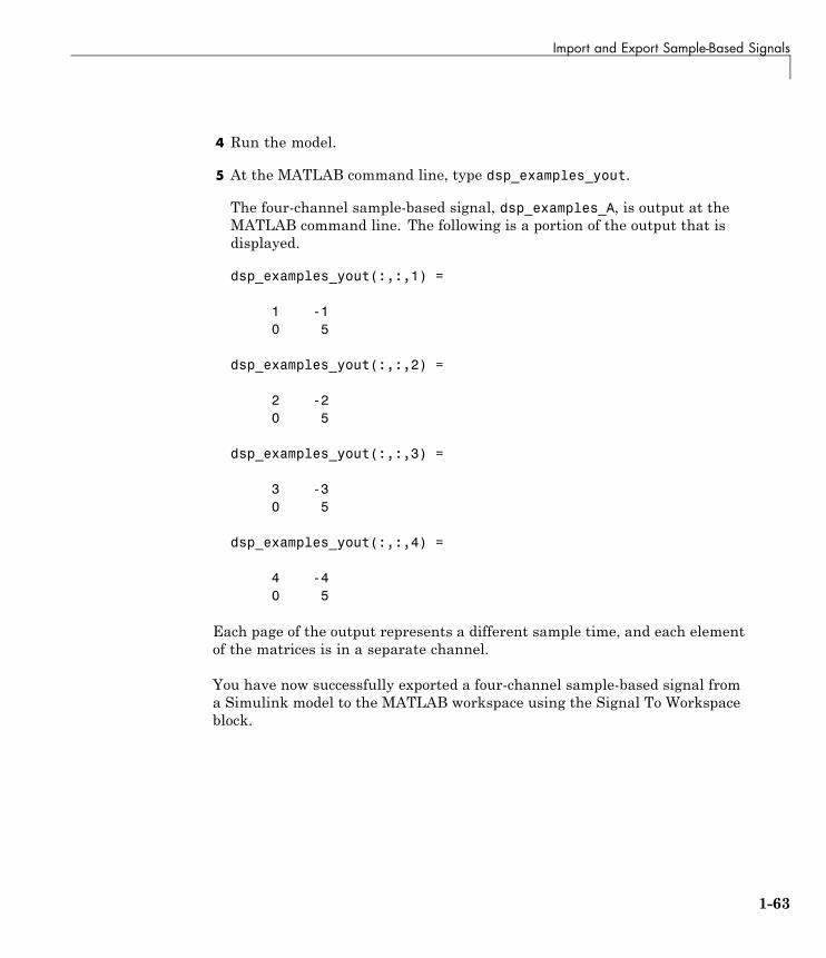
Import and Export Sample-Based Signals
4 Run the model.
5 At the MATLAB command line, type dsp_examples_yout.
The four-channel sample-based signal, dsp_examples_A, is output at theMATLAB command line. The following is a portion of the output that isdisplayed.
dsp_examples_yout(:,:,1) =
1 -10 5
dsp_examples_yout(:,:,2) =
2 -20 5
dsp_examples_yout(:,:,3) =
3 -30 5
dsp_examples_yout(:,:,4) =
4 -40 5
Each page of the output represents a different sample time, and each elementof the matrices is in a separate channel.
You have now successfully exported a four-channel sample-based signal froma Simulink model to the MATLAB workspace using the Signal To Workspaceblock.
1-63
1 Input, Output, and Display
Import and Export Frame-Based Signals
Note Starting in R2010b, many DSP System Toolbox blocks received a newparameter to control whether they perform sample- or frame-based processing.The following content has not been updated to reflect this change. For moreinformation, see the “Frame-Based Processing” section of the Release Notes.
In this section...
“Import Frame-Based Signals” on page 1-64
“Export Frame-Based Signals” on page 1-67
Import Frame-Based SignalsThe Signal From Workspace block creates a frame-based multichannel signalwhen the Signal parameter is a matrix, and the Samples per frameparameter, M, is greater than 1. Beginning with the first M rows of thematrix, the block releases M rows of the matrix (that is, one frame from eachchannel) to the output port every M*Ts seconds. Therefore, if the Signalparameter specifies a W-by-N workspace matrix, the Signal From Workspaceblock outputs a series of M-by-N matrices representing N channels. Theworkspace matrix must be oriented so that its columns represent the channelsof the signal.
The figure below is a graphical illustration of this process for a 6-by-4workspace matrix, A, and a frame size of 2.
1-64
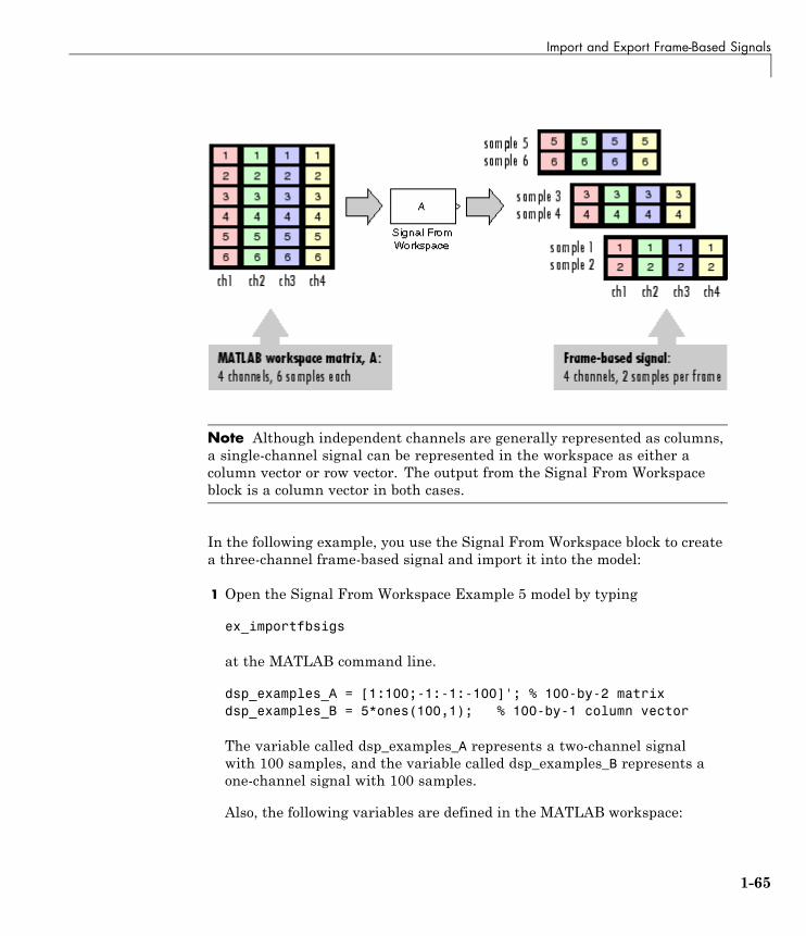
Import and Export Frame-Based Signals
Note Although independent channels are generally represented as columns,a single-channel signal can be represented in the workspace as either acolumn vector or row vector. The output from the Signal From Workspaceblock is a column vector in both cases.
In the following example, you use the Signal From Workspace block to createa three-channel frame-based signal and import it into the model:
1 Open the Signal From Workspace Example 5 model by typing
ex_importfbsigs
at the MATLAB command line.
dsp_examples_A = [1:100;-1:-1:-100]'; % 100-by-2 matrixdsp_examples_B = 5*ones(100,1); % 100-by-1 column vector
The variable called dsp_examples_A represents a two-channel signalwith 100 samples, and the variable called dsp_examples_B represents aone-channel signal with 100 samples.
Also, the following variables are defined in the MATLAB workspace:
1-65

1 Input, Output, and Display
2 Double-click the Signal From Workspace block. Set the block parametersas follows, and then click OK:
• Signal parameter to [dsp_examples_A dsp_examples_B]
• Sample time parameter to 1
• Samples per frame parameter to 4
• Form output after final data value parameter to Setting to zero
1-66

Import and Export Frame-Based Signals
Based on these parameters, the Signal From Workspace block outputsa frame-based signal with a frame size of 4 and a sample period of 1second. The signal’s frame period is 4 seconds. The Signal parameteruses the standard MATLAB syntax for horizontally concatenatingmatrices to append column vector dsp_examples_B to the right of matrixdsp_examples_A. After the block has output the signal, all subsequentoutputs have a value of zero.
3 Run the model.
The figure below is a graphical representation of how your three-channel,frame-based signal is imported into your model.
You have now successfully imported a three-channel frame-based signal intoyour model using the Signal From Workspace block.
Export Frame-Based SignalsThe Signal To Workspace and Triggered To Workspace blocks are the primaryblocks for exporting signals of all dimensions from a Simulink model to theMATLAB workspace.
A frame-based signal with N channels and frame size M is represented by asequence of M-by-N matrices. When the input to the Signal To Workspaceblock is a frame-based signal, the block creates a P-by-N array in the MATLABworkspace containing the P most recent samples from each channel. The
1-67
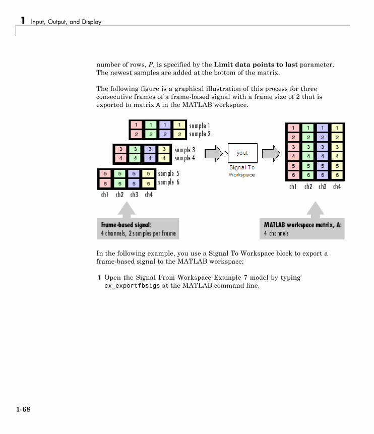
1 Input, Output, and Display
number of rows, P, is specified by the Limit data points to last parameter.The newest samples are added at the bottom of the matrix.
The following figure is a graphical illustration of this process for threeconsecutive frames of a frame-based signal with a frame size of 2 that isexported to matrix A in the MATLAB workspace.
In the following example, you use a Signal To Workspace block to export aframe-based signal to the MATLAB workspace:
1 Open the Signal From Workspace Example 7 model by typingex_exportfbsigs at the MATLAB command line.
1-68
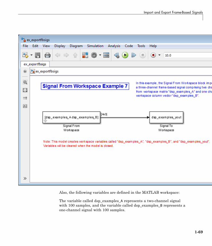
Import and Export Frame-Based Signals
Also, the following variables are defined in the MATLAB workspace:
The variable called dsp_examples_A represents a two-channel signalwith 100 samples, and the variable called dsp_examples_B represents aone-channel signal with 100 samples.
1-69

1 Input, Output, and Display
dsp_examples_A = [1:100;-1:-1:-100]'; % 100-by-2 matrixdsp_examples_B = 5*ones(100,1); % 100-by-1 column vector
2 Double-click the Signal From Workspace block. Set the block parametersas follows, and then click OK:
• Signal = [dsp_examples_A dsp_examples_B]
• Sample time = 1
• Samples per frame = 4
• Form output after final data value = Setting to zero
Based on these parameters, the Signal From Workspace block outputsa frame-based signal with a frame size of 4 and a sample period of 1second. The signal’s frame period is 4 seconds. The Signal parameteruses the standard MATLAB syntax for horizontally concatenatingmatrices to append column vector dsp_examples_B to the right of matrixdsp_examples_A. After the block has output the signal, all subsequentoutputs have a value of zero.
3 Double-click the Signal To Workspace block. Set the block parameters asfollows, and then click OK:
• Variable name = dsp_examples_yout
• Limit data points to last = inf
• Decimation = 1
• Frames = Concatenate frames (2-D array)
Based on these parameters, the Signal To Workspace block exports itsframe-based input signal to a variable called dsp_examples_yout in theMATLAB workspace. The workspace variable can grow indefinitely largein order to capture all of the input data. The signal is not decimated beforeit is exported to the MATLAB workspace, and each input frame is verticallyconcatenated to the previous frame to produce a 2-D array output.
4 Run the model.
The following figure is a graphical representation of the model’s behaviorduring simulation.
1-70
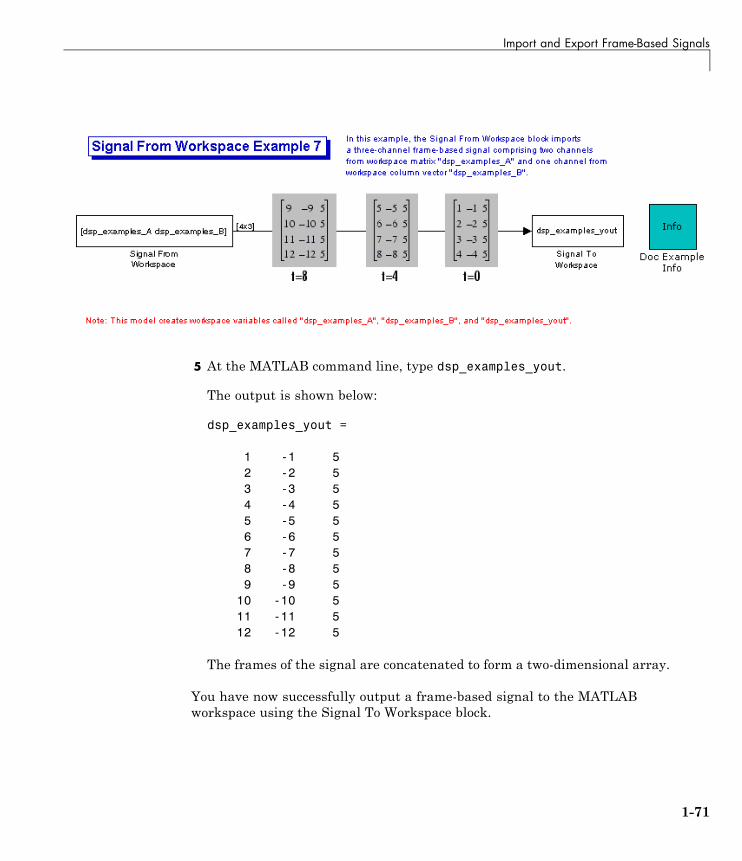
Import and Export Frame-Based Signals
5 At the MATLAB command line, type dsp_examples_yout.
The output is shown below:
dsp_examples_yout =
1 -1 52 -2 53 -3 54 -4 55 -5 56 -6 57 -7 58 -8 59 -9 5
10 -10 511 -11 512 -12 5
The frames of the signal are concatenated to form a two-dimensional array.
You have now successfully output a frame-based signal to the MATLABworkspace using the Signal To Workspace block.
1-71
1 Input, Output, and Display
Musical Instrument Digital Interface
In this section...
“About MIDI” on page 1-72
“MIDI Control Surfaces” on page 1-72
“Using MIDI Control Surfaces with MATLAB and Simulink” on page 1-73
About MIDIThe Musical Instrument Digital Interface (MIDI) was originally developed tointerconnect electronic musical instruments. This interface is very flexibleand has many uses in many applications far beyond musical instruments.Its simple unidirectional messaging protocol supports many different kindsof messaging.
Windows, Macintosh, and Linux platforms all have native support for MIDI,so software on any of these platforms can send and receive MIDI messages.See http://www.midi.org for more information about MIDI.
MIDI Control SurfacesOne kind of MIDI message is the Control Change message, used tocommunicate changes in controls, such as knobs, sliders, and buttons. AMIDI Control Surface is a device with controls that sends MIDI ControlChange messages when you turn a knob, move a slider, or push a buttonon a MIDI control surface. This Control Change message indicates whichcontrol changed and what its new position is. MIDI control surfaces arequite generic because the interpretation of the Control Change message isentirely up to the message recipient. Even though some control surfaces aretailored for particular applications, the messages they send can be used tocontrol anything.
Hardware MIDI control surfaces are widely available in a range ofconfigurations and prices. MIDI control apps can turn a smartphone or tabletinto a virtual MIDI control surface. For custom applications, MIDI controlsurfaces are not difficult to build using, for example, Arduino boards.
1-72
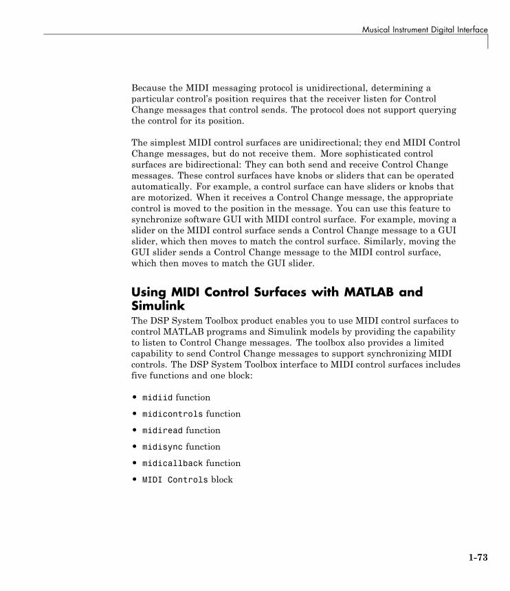
Musical Instrument Digital Interface
Because the MIDI messaging protocol is unidirectional, determining aparticular control’s position requires that the receiver listen for ControlChange messages that control sends. The protocol does not support queryingthe control for its position.
The simplest MIDI control surfaces are unidirectional; they end MIDI ControlChange messages, but do not receive them. More sophisticated controlsurfaces are bidirectional: They can both send and receive Control Changemessages. These control surfaces have knobs or sliders that can be operatedautomatically. For example, a control surface can have sliders or knobs thatare motorized. When it receives a Control Change message, the appropriatecontrol is moved to the position in the message. You can use this feature tosynchronize software GUI with MIDI control surface. For example, moving aslider on the MIDI control surface sends a Control Change message to a GUIslider, which then moves to match the control surface. Similarly, moving theGUI slider sends a Control Change message to the MIDI control surface,which then moves to match the GUI slider.
Using MIDI Control Surfaces with MATLAB andSimulinkThe DSP System Toolbox product enables you to use MIDI control surfaces tocontrol MATLAB programs and Simulink models by providing the capabilityto listen to Control Change messages. The toolbox also provides a limitedcapability to send Control Change messages to support synchronizing MIDIcontrols. The DSP System Toolbox interface to MIDI control surfaces includesfive functions and one block:
• midiid function
• midicontrols function
• midiread function
• midisync function
• midicallback function
• MIDI Controls block
1-73

1 Input, Output, and Display
Initial SetupYour MIDI control surface should be connected to your computer, and turnedon, before starting MATLAB. Instructions for connecting your MIDI device toyour computer vary from device to device. See the instructions that came withyour particular device. If you start MATLAB before connecting your device,MATLAB may not recognize your device when you connect it. To correct theproblem, restart MATLAB with the device already connected.
Next, set the MATLAB preference, specifying the name of the default MIDIdevice. Use midiid to determine the name of the device, and then usesetpref to set the preference:
>> [control, device] = midiidMove the control you wish to identify; type ^C to abort.Waiting for control message... donecontrol =
1082device =BCF2000>> setpref('midi', 'DefaultDevice', device)>>
This preference persists across MATLAB sessions, so you only have to set itonce, unless you want to change devices.
If you do not set this preference, MATLAB and the host operating systemchoose a device for you. However, such autoselection can cause unpredictableresults because many computers have “virtual” (software) MIDI devicesinstalled that you may not be aware of. For predictable behavior, you shouldset the preference.
You can always override this default and explicitly specify a device name.Thus, you can use multiple MIDI devices simultaneously.
Identifying ControlsBefore you can connect a MIDI control with MATLAB or Simulink, you mustknow the identifiers for that particular control:
• Control number
1-74
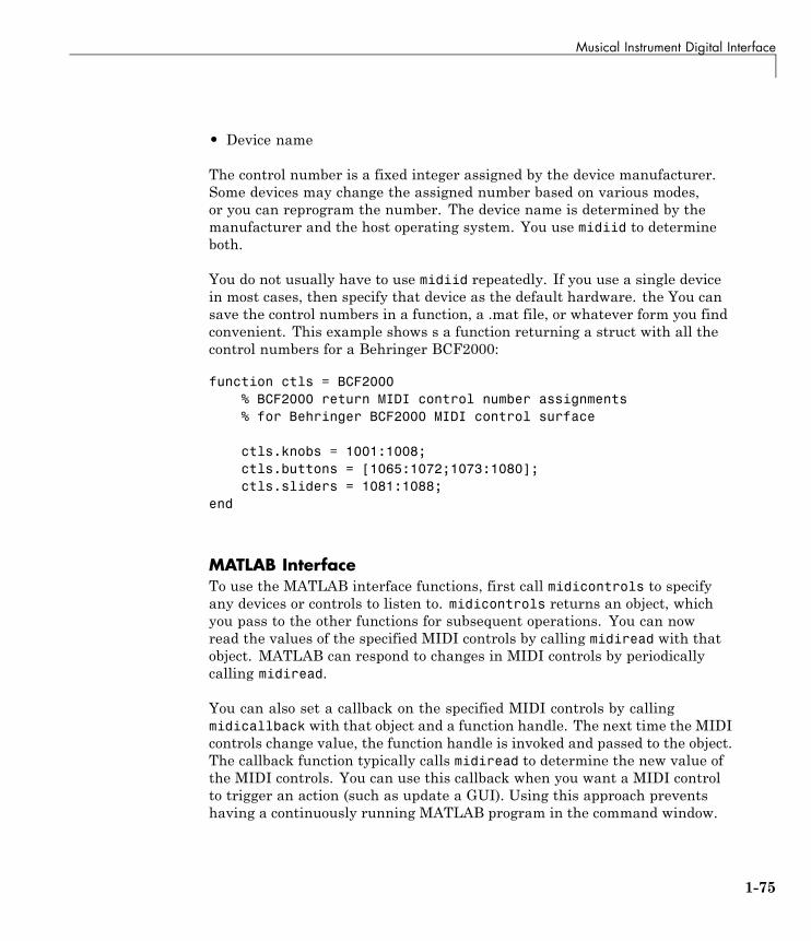
Musical Instrument Digital Interface
• Device name
The control number is a fixed integer assigned by the device manufacturer.Some devices may change the assigned number based on various modes,or you can reprogram the number. The device name is determined by themanufacturer and the host operating system. You use midiid to determineboth.
You do not usually have to use midiid repeatedly. If you use a single devicein most cases, then specify that device as the default hardware. the You cansave the control numbers in a function, a .mat file, or whatever form you findconvenient. This example shows s a function returning a struct with all thecontrol numbers for a Behringer BCF2000:
function ctls = BCF2000% BCF2000 return MIDI control number assignments% for Behringer BCF2000 MIDI control surface
ctls.knobs = 1001:1008;ctls.buttons = [1065:1072;1073:1080];ctls.sliders = 1081:1088;
end
MATLAB InterfaceTo use the MATLAB interface functions, first call midicontrols to specifyany devices or controls to listen to. midicontrols returns an object, whichyou pass to the other functions for subsequent operations. You can nowread the values of the specified MIDI controls by calling midiread with thatobject. MATLAB can respond to changes in MIDI controls by periodicallycalling midiread.
You can also set a callback on the specified MIDI controls by callingmidicallback with that object and a function handle. The next time the MIDIcontrols change value, the function handle is invoked and passed to the object.The callback function typically calls midiread to determine the new value ofthe MIDI controls. You can use this callback when you want a MIDI controlto trigger an action (such as update a GUI). Using this approach preventshaving a continuously running MATLAB program in the command window.
1-75
1 Input, Output, and Display
SynchronizationIf midiread is called before the MIDI control sends a Control Changemessage, the midicontrols object has no information about the actual stateof the MIDI control. During this time, the midicontrols object and the actualMIDI control are out of sync with each other. Thus, calling midiread returnsthe initial value that was specified in the call to midicontrols (0 by default).You can synchronize the object with the control by moving the MIDI control.The MIDI control responds by sending a Control Change message causing themidicontrols object to sync to the MIDI control. If your MIDI control surface isbidirectional, you can sync in the other direction by calling midisync to sendthe midicontrols object’s initial value to the actual MIDI control. The MIDIcontrol responds by moving into sync with the midicontrols object.
It is generally harmless to call midisync even if the MIDI control surface isnot bidirectional, so it is usually good practice to call midisync immediatelyafter calling midicontrols.
Synchronization is also useful to link a MIDI control with a GUI control (auicontrol slider, for example), so that when one control is changed, the othercontrol tracks it. Typically, you implement such tracking by setting callbackfunctions on both the MIDI control (using midicallback) and the GUI control.The MIDI control callback sends its new value to the GUI control and the GUIcontrol sends its value to the MIDI control, using midisync.
Simulink InterfaceThe MIDI Controls block provides the Simulink interface. See the blockreference page MIDI Controls for more details.
1-76

Display Time-Domain Data
Display Time-Domain Data
In this section...
“Configure the Time Scope Properties” on page 1-78
“Use the Simulation Controls” on page 1-85
“Modify the Time Scope Display” on page 1-86
“Inspect Your Data (Scaling the Axes and Zooming)” on page 1-88
“Manage Multiple Time Scopes” on page 1-91
The following tutorial shows you how to configure the Time Scope blocks inthe ex_timescope_tut model to display time-domain signals. To get startedwith this tutorial, open the model by typing
ex_timescope_tut
at the MATLAB command line.
1-77
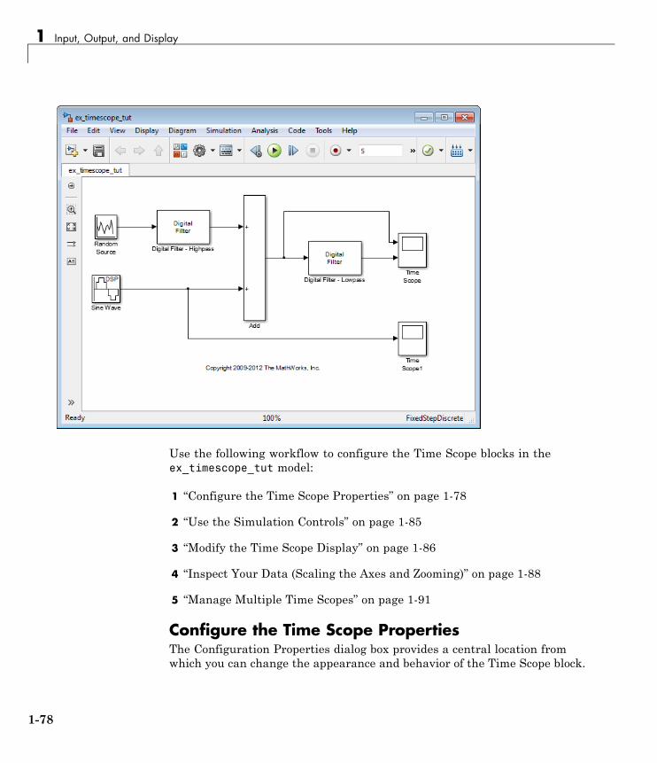
1 Input, Output, and Display
Use the following workflow to configure the Time Scope blocks in theex_timescope_tut model:
1 “Configure the Time Scope Properties” on page 1-78
2 “Use the Simulation Controls” on page 1-85
3 “Modify the Time Scope Display” on page 1-86
4 “Inspect Your Data (Scaling the Axes and Zooming)” on page 1-88
5 “Manage Multiple Time Scopes” on page 1-91
Configure the Time Scope PropertiesThe Configuration Properties dialog box provides a central location fromwhich you can change the appearance and behavior of the Time Scope block.
1-78

Display Time-Domain Data
To open the Configuration Properties dialog box, you must first open the TimeScope window by double-clicking the Time Scope block in your model. Whenthe window opens, select View > Configuration Properties. Alternatively,
in the Time Scope toolbar, click the Configuration Properties button.
The Configuration Properties dialog box has four different tabs,Main, Time,Display, and Logging, each of which offers you a different set of options.For more information about the options available on each of the tabs, seethe Time Scope block reference page.
Note As you progress through this workflow, notice the blue question mark
icon ( ) in the lower-left corner of the subsequent dialog boxes. Thisicon indicates that context-sensitive help is available. You can get moreinformation about any of the parameters on the dialog box by right-clickingthe parameter name and selecting What’s This?
1-79
1 Input, Output, and Display
Configure Appearance and Specify Signal InterpretationFirst, you configure the appearance of the Time Scope window and specifyhow the Time Scope block should interpret input signals. In the ConfigurationProperties dialog box, click theMain tab. Choose the appropriate parametersettings for the Main tab, as shown in the following table.
Parameter Setting
Open atsimulationstart
Checked
Number ofinput ports
2
Inputprocessing
Columns as channels (frame based)
Maximizeaxes
Auto
Axes scaling Manual
In this tutorial, you want the block to treat the input signal as frame-based,so you must set the Input processing parameter to Columns as channels(frame based).
Configure Axes Scaling and Data AlignmentThe Main tab also allows you to control when and how Time Scope scalesthe axes. These options also control how Time Scope aligns your data withrespect to the axes. Click the link labeled Configure... to the right of theAxes scaling parameter to see additional options for axes scaling. After youclick this button, the label changes to Hide... and new parameters appear.The following table describes these additional options.
1-80
Display Time-Domain Data
Parameter Description
Axes scaling Specify when the scope should automatically scale theaxes. You can select one of the following options:
• Manual — When you select this option, the scope doesnot automatically scale the axes. You can manuallyscale the axes in any of the following ways:
- Select Tools > Axes Scaling Properties.
- Press one of the Scale Axis Limits toolbar buttons.
- When the scope figure is the active window, pressCtrl and A simultaneously.
• Auto — When you select this option, the scope scalesthe axes as needed, both during and after simulation.Selecting this option shows the Do not allow Y-axislimits to shrink check box.
• After N Updates — Selecting this option causes thescope to scale the axes after a specified number ofupdates. Selecting this option shows the Number ofupdates edit box.
By default, this property is set to Auto. This property isTunable.
Scale axeslimits at stop
Select this check box to scale the axes when the simulationstops. The y-axis is always scaled. The x-axis limits areonly scaled if you also select the Scale X-axis limitscheck box.
1-81
1 Input, Output, and Display
Parameter Description
Data range(%)
Allows you to specify how much white space surroundsyour signal in the Time Scope window. You can specify avalue for both the y- and x-axis. The higher the value youenter for the y-axis Data range (%), the tighter the y-axisrange is with respect to the minimum and maximumvalues in your signal. For example, to have your signalcover the entire y-axis range when the block scales theaxes, set this value to 100.
Align Allows you to specify where the block should align yourdata with respect to each axis. You can choose to haveyour data aligned with the top, bottom, or center of they-axis. Additionally, if you select the Autoscale X-axislimits check box, you can choose to have your data alignedwith the right, left, or center of the x-axis.
Set the parameters to the values shown in the following table.
Parameter Setting
Axes scaling Manual
Scale axeslimits at stop
Checked
Data range(%)
80
Align Center
AutoscaleX-axis limits
Unchecked
Set Time Domain PropertiesIn the Configuration Properties dialog box, click the Time tab. Set theparameters to the values shown in the following table.
1-82
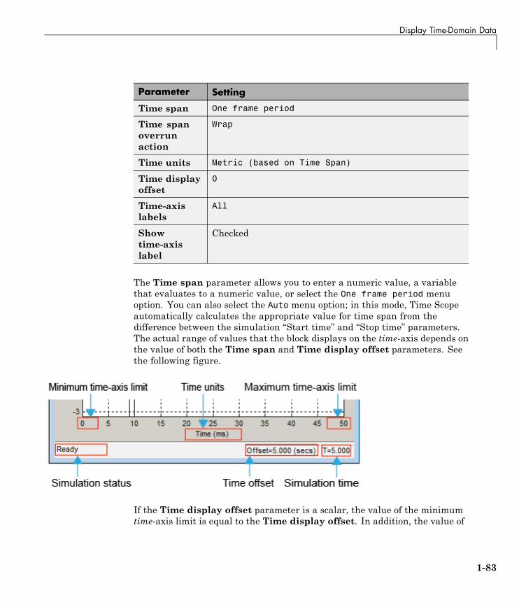
Display Time-Domain Data
Parameter Setting
Time span One frame period
Time spanoverrunaction
Wrap
Time units Metric (based on Time Span)
Time displayoffset
0
Time-axislabels
All
Showtime-axislabel
Checked
The Time span parameter allows you to enter a numeric value, a variablethat evaluates to a numeric value, or select the One frame period menuoption. You can also select the Auto menu option; in this mode, Time Scopeautomatically calculates the appropriate value for time span from thedifference between the simulation “Start time” and “Stop time” parameters.The actual range of values that the block displays on the time-axis depends onthe value of both the Time span and Time display offset parameters. Seethe following figure.
If the Time display offset parameter is a scalar, the value of the minimumtime-axis limit is equal to the Time display offset. In addition, the value of
1-83

1 Input, Output, and Display
the maximum time-axis limit is equal to the sum of the Time display offsetparameter and the Time span parameter. For information on the otherparameters in the Time Scope window, see the Time Scope reference page.
In this tutorial, the values on the time-axis range from 0 to One frameperiod, where One frame period is 0.05 seconds (50 ms).
Set Display PropertiesIn the Configuration Properties dialog box, click the Display tab. Set theparameters to the values shown in the following table.
Parameter Setting
Active display 1
Title
Show legend Checked
Show grid Checked
Plot signal(s) as magnitude andphase
Unchecked
Y-limits (Minimum) -2.5
Y-limits (Maximum) 2.5
Y-label Amplitude
Set Logging PropertiesIn the Configuration Properties dialog box, click the Logging tab. Set Logdata to workspace to unchecked.
Click OK to save your changes and close the Configuration Properties dialogbox.
Note If you have not already done so, repeat all of these procedures for theTime Scope1 block (except leave the Number of input ports on the Maintab as 1) before continuing with the other sections of this tutorial.
1-84
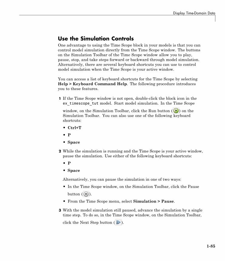
Display Time-Domain Data
Use the Simulation ControlsOne advantage to using the Time Scope block in your models is that you cancontrol model simulation directly from the Time Scope window. The buttonson the Simulation Toolbar of the Time Scope window allow you to play,pause, stop, and take steps forward or backward through model simulation.Alternatively, there are several keyboard shortcuts you can use to controlmodel simulation when the Time Scope is your active window.
You can access a list of keyboard shortcuts for the Time Scope by selectingHelp > Keyboard Command Help. The following procedure introducesyou to these features.
1 If the Time Scope window is not open, double-click the block icon in theex_timescope_tut model. Start model simulation. In the Time Scope
window, on the Simulation Toolbar, click the Run button ( ) on theSimulation Toolbar. You can also use one of the following keyboardshortcuts:
• Ctrl+T
• P
• Space
2 While the simulation is running and the Time Scope is your active window,pause the simulation. Use either of the following keyboard shortcuts:
• P
• Space
Alternatively, you can pause the simulation in one of two ways:
• In the Time Scope window, on the Simulation Toolbar, click the Pause
button ( ).
• From the Time Scope menu, select Simulation > Pause.
3 With the model simulation still paused, advance the simulation by a singletime step. To do so, in the Time Scope window, on the Simulation Toolbar,
click the Next Step button ( ).
1-85
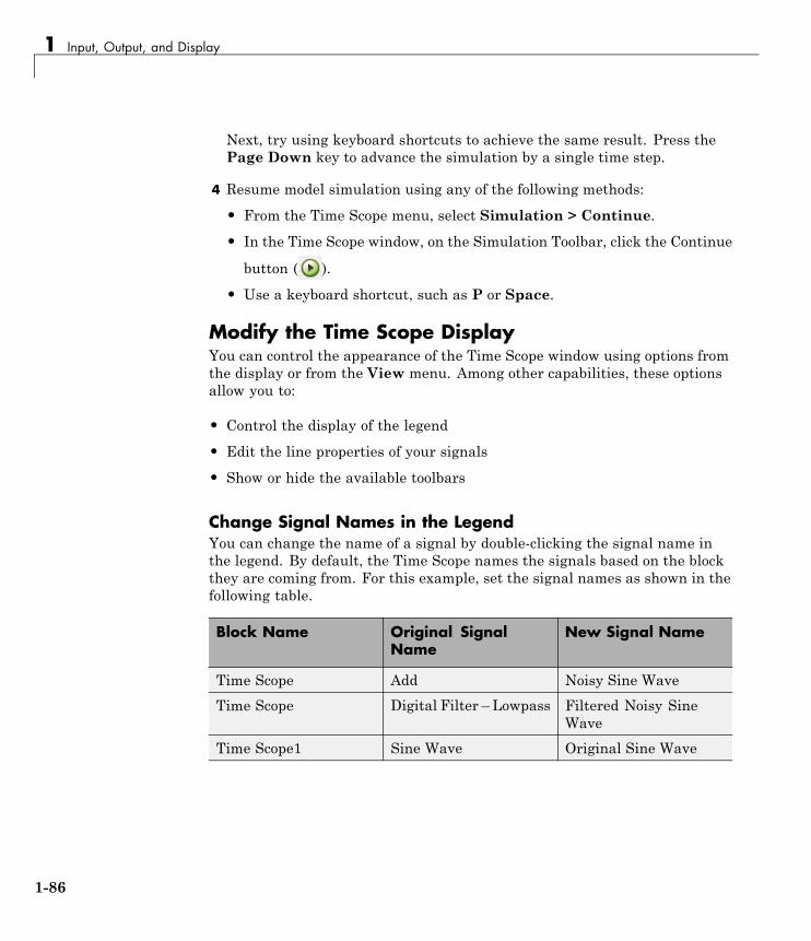
1 Input, Output, and Display
Next, try using keyboard shortcuts to achieve the same result. Press thePage Down key to advance the simulation by a single time step.
4 Resume model simulation using any of the following methods:
• From the Time Scope menu, select Simulation > Continue.
• In the Time Scope window, on the Simulation Toolbar, click the Continue
button ( ).
• Use a keyboard shortcut, such as P or Space.
Modify the Time Scope DisplayYou can control the appearance of the Time Scope window using options fromthe display or from the View menu. Among other capabilities, these optionsallow you to:
• Control the display of the legend
• Edit the line properties of your signals
• Show or hide the available toolbars
Change Signal Names in the LegendYou can change the name of a signal by double-clicking the signal name inthe legend. By default, the Time Scope names the signals based on the blockthey are coming from. For this example, set the signal names as shown in thefollowing table.
Block Name Original SignalName
New Signal Name
Time Scope Add Noisy Sine Wave
Time Scope Digital Filter – Lowpass Filtered Noisy SineWave
Time Scope1 Sine Wave Original Sine Wave
1-86
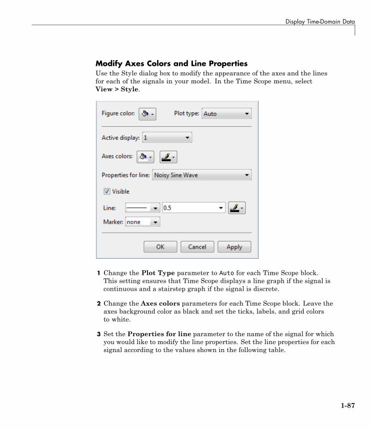
Display Time-Domain Data
Modify Axes Colors and Line PropertiesUse the Style dialog box to modify the appearance of the axes and the linesfor each of the signals in your model. In the Time Scope menu, selectView > Style.
1 Change the Plot Type parameter to Auto for each Time Scope block.This setting ensures that Time Scope displays a line graph if the signal iscontinuous and a stairstep graph if the signal is discrete.
2 Change the Axes colors parameters for each Time Scope block. Leave theaxes background color as black and set the ticks, labels, and grid colorsto white.
3 Set the Properties for line parameter to the name of the signal for whichyou would like to modify the line properties. Set the line properties for eachsignal according to the values shown in the following table.
1-87
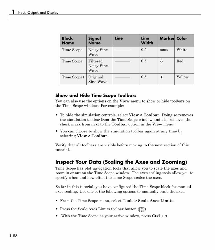
1 Input, Output, and Display
BlockName
SignalName
Line LineWidth
Marker Color
Time Scope Noisy SineWave
———— 0.5 none White
Time Scope FilteredNoisy SineWave
———— 0.5 Red
Time Scope1 OriginalSine Wave
———— 0.5 Yellow
Show and Hide Time Scope ToolbarsYou can also use the options on the View menu to show or hide toolbars onthe Time Scope window. For example:
• To hide the simulation controls, select View > Toolbar. Doing so removesthe simulation toolbar from the Time Scope window and also removes thecheck mark from next to the Toolbar option in the View menu.
• You can choose to show the simulation toolbar again at any time byselecting View > Toolbar.
Verify that all toolbars are visible before moving to the next section of thistutorial.
Inspect Your Data (Scaling the Axes and Zooming)Time Scope has plot navigation tools that allow you to scale the axes andzoom in or out on the Time Scope window. The axes scaling tools allow you tospecify when and how often the Time Scope scales the axes.
So far in this tutorial, you have configured the Time Scope block for manualaxes scaling. Use one of the following options to manually scale the axes:
• From the Time Scope menu, select Tools > Scale Axes Limits.
• Press the Scale Axes Limits toolbar button ( ).
• With the Time Scope as your active window, press Ctrl + A.
1-88
Display Time-Domain Data
Adjust White Space Around the SignalYou can control how much space surrounds your signal and where your signalappears in relation to the axes. To adjust the amount of space surroundingyour signal and realign it with the axes, you must first open the Tools—PlotNavigation Properties dialog box. From the Time Scope menu, selectTools > Axes Scaling Properties .
In the Tools:Plot Navigation options dialog box, set the Data range (%) andAlign parameters. In a previous section, you set these parameters to 80 andCenter, respectively.
• To decrease the amount of space surrounding your signal, set the Datarange (%) parameter on the Tools:Plot Navigation Options dialog box to 90.
• To align your signal with the bottom of the Y-axis, set the Align parameterto Bottom.
The next time you scale the axes of the Time Scope window, the windowappears as follows.
1-89

1 Input, Output, and Display
1-90

Display Time-Domain Data
Use the Zoom ToolsThe zoom tools allow you to zoom in simultaneously in the directions of boththe x- and y-axes , or in either direction individually. For example, to zoom inon the signal between 5010 ms and 5020 ms, you can use the Zoom X option.
• To activate the Zoom X tool, select Tools > Zoom X, or press the
corresponding toolbar button ( ). The Time Scope indicates that theZoom X tool is active by depressing the toolbar button and placing a checkmark next to the Tools > Zoom X menu option.
• To zoom in on the region between 5010 ms and 5020 ms, in the Time Scopewindow, click and drag your cursor from the 10 ms mark to the 20 ms mark.
• While zoomed in, to activate the Pan tool, select Tools > Pan, or press the
corresponding toolbar button ( ).
• To zoom out of the Time Scope window, right-click inside the window, andselect Zoom Out. Alternatively, you can return to the original view ofyour signal by right-clicking inside the Time Scope window and selectingReset to Original View.
Manage Multiple Time ScopesThe Time Scope block provides tools to help you manage multiple TimeScope blocks in your models. The model used throughout this tutorial,ex_timescope_tut, contains two Time Scope blocks, labeled Time Scope andTime Scope1. The following sections discuss the tools you can use to managethese Time Scope blocks.
Open All Time Scope WindowsWhen you have multiple windows open on your desktop, finding the oneyou need can be difficult. The Time Scope block offers a View > Bring AllTime Scopes Forward menu option to help you manage your Time Scopewindows. Selecting this option brings all Time Scope windows into view. Ifa Time Scope window is not currently open, use this menu option to openthe window and bring it into view.
To try this menu option in the ex_timescope_tut model, open the TimeScope window, and close the Time Scope1 window. From the View menu ofthe Time Scope window, select Bring All Time Scopes Forward. The Time
1-91
1 Input, Output, and Display
Scope1 window opens, along with the already active Time Scope window. Ifyou have any Time Scope blocks in other open Simulink models, then thesealso come into view.
Open Time Scope Windows at Simulation StartWhen you have multiple Time Scope blocks in your model, you may not wantall Time Scope windows to automatically open when you start simulation.You can control whether or not the Time Scope window opens at simulationstart by selecting File > Open at Start of Simulation from the TimeScope window. When you select this option, the Time Scope GUI opensautomatically when you start the simulation. When you do not select thisoption, you must manually open the scope window by double-clicking thecorresponding Time Scope block in your model.
Find the Right Time Scope Block in Your ModelSometimes, you have multiple Time Scope blocks in your model and need tofind the location of one that corresponds to the active Time Scope window. Insuch cases, you can use the View > Highlight Simulink Block menu option
or the corresponding toolbar button ( ). When you do so, the model windowbecomes your active window, and the corresponding Time Scope block flashesthree times in the model window. This option can help you locate Time Scopeblocks in your model and determine to which signals they are attached.
To try this feature, open the Time Scope window, and on the simulationtoolbar, click the Highlight Simulink Block button. Doing so opens theex_timescope_tut model. The Time Scope block flashes three times in themodel window, allowing you to see where in your model the block of interest islocated.
Docking Time Scope Windows in the Scopes Group ContainerWhen you have multiple Time Scope blocks in your model you may want tosee them in the same window and compare them side-by-side. In such cases,you can select the Dock Time Scope button ( ) at the top-right corner of theTime Scope window for the Time Scope block.
1-92

Display Time-Domain Data
The Time Scope window now appears in the Scopes group container. Next,press the Dock Time Scope button at the top-right corner of the Time Scopewindow for the Time Scope1 block.
By default, the Scopes group container is situated above the MATLABCommand Window. However, you can undock the Scopes group container by
pressing the Show Actions button ( ) at the top-right corner of the containerand selecting Undock. The Scopes group container is now independent fromthe MATLAB Command Window.
1-93
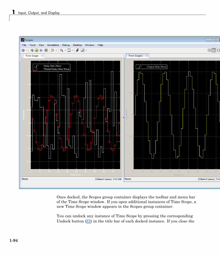
1 Input, Output, and Display
Once docked, the Scopes group container displays the toolbar and menu barof the Time Scope window. If you open additional instances of Time Scope, anew Time Scope window appears in the Scopes group container.
You can undock any instance of Time Scope by pressing the correspondingUndock button ( ) in the title bar of each docked instance. If you close the
1-94
Display Time-Domain Data
Scopes group container, all docked instances of Time Scope close but theSimulink model continues to run.
tFor more information on docking figures, see “Docking Figures in theDesktop” in the MATLAB documentation.
Close All Time Scope WindowsIf you save your model with Time Scope windows open, those windows willreopen the next time you open the model. Reopening the Time Scope windowswhen you open your model can increase the amount of time it takes yourmodel to load. If you are working with a large model, or a model containingmultiple Time Scopes, consider closing all Time Scope windows before yousave and close that model. To do so, use the File > Close All Time ScopeWindows menu option.
To use this menu option in the ex_timescope_tut model, open the TimeScope or Time Scope1 window, and select File > Close All Time ScopeWindows. Both the Time Scope and Time Scope1 windows close. If you nowsave and close the model, the Time Scope windows do not automatically openthe next time you open the model. You can open Time Scope windows at anytime by double-clicking a Time Scope block in your model. Alternatively,you can choose to automatically open the Time Scope windows at simulationstart. To do so, from the Time Scope window, select File > Open at Startof Simulation.
1-95
1 Input, Output, and Display
Display Frequency-Domain Data in Spectrum AnalyzerYou can use DSP System Toolbox blocks to work with signals in both the timeand frequency domain. To display frequency-domain signals, you can useblocks from the Sinks library, such as the Vector Scope, Spectrum Analyzer,Matrix Viewer, and Waterfall Scope blocks.
With the Spectrum Analyzer block, you can display the frequency spectra oftime-domain input data. In contrast to the Vector Scope block, the SpectrumAnalyzer block computes the Fast Fourier Transform (FFT) of the input signalinternally, transforming the signal into the frequency domain.
This example shows how you can use a Spectrum Analyzer block to displaythe frequency content of two frame-based signals simultaneously:
1 At the MATLAB command prompt, type ex_spectrumanalyzer_tut.
The Spectrum Analyzer example opens, and the variables, Fs and mtlb, areloaded into the MATLAB workspace.
1-96
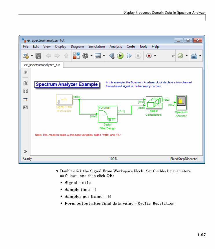
Display Frequency-Domain Data in Spectrum Analyzer
2 Double-click the Signal From Workspace block. Set the block parametersas follows, and then click OK:
• Signal = mtlb
• Sample time = 1
• Samples per frame = 16
• Form output after final data value = Cyclic Repetition
1-97

1 Input, Output, and Display
Based on these parameters, the Signal From Workspace block repeatedlyoutputs the input signal, mtlb, as a frame-based signal with a sampleperiod of 1 second.
3 Create two distinct signals to send to the Spectrum Analyzer block. Usethe Digital Filter Design block to filter the input signal, using the defaultparameters.
1-98

Display Frequency-Domain Data in Spectrum Analyzer
4 Double-click the Matrix Concatenate block. Set the block parameters asfollows, and then click OK:
• Number of inputs = 2
• Mode = Multidimensional array
1-99
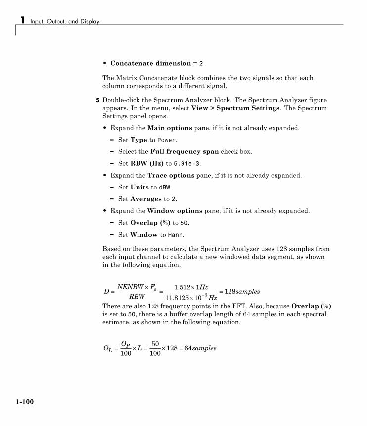
1 Input, Output, and Display
• Concatenate dimension = 2
The Matrix Concatenate block combines the two signals so that eachcolumn corresponds to a different signal.
5 Double-click the Spectrum Analyzer block. The Spectrum Analyzer figureappears. In the menu, select View > Spectrum Settings. The SpectrumSettings panel opens.
• Expand theMain options pane, if it is not already expanded.
– Set Type to Power.
– Select the Full frequency span check box.
– Set RBW (Hz) to 5.91e-3.
• Expand the Trace options pane, if it is not already expanded.
– Set Units to dBW.
– Set Averages to 2.
• Expand theWindow options pane, if it is not already expanded.
– Set Overlap (%) to 50.
– Set Window to Hann.
Based on these parameters, the Spectrum Analyzer uses 128 samples fromeach input channel to calculate a new windowed data segment, as shownin the following equation.
DNENBW F
RBWHz
Hzsampless
1 512 1
11 8125 10128
3.
.There are also 128 frequency points in the FFT. Also, because Overlap (%)is set to 50, there is a buffer overlap length of 64 samples in each spectralestimate, as shown in the following equation.
OO
L samplesLP
10050
100128 64
1-100

Display Frequency-Domain Data in Spectrum Analyzer
Every time the scope updates the display, 64 points are plotted for eachchannel. At 16 samples per frame, Spectrum Analyzer waits for 3 frames or48 samples before displaying the first power spectral estimate.
6 Fit all the calculated data points into the display. In the Spectrum Analyzermenu, select Tools > Automatically Scale Axes Limits.
7 In the Spectrum Analyzer menu, select View > ConfigurationProperties. Then, select the Show legend check box.
8 Run the model. The Spectrum Analyzer block computes the FFT ofeach of the input signals. It then displays the power spectra of thefrequency-domain signals in the Spectrum Analyzer window.
1-101
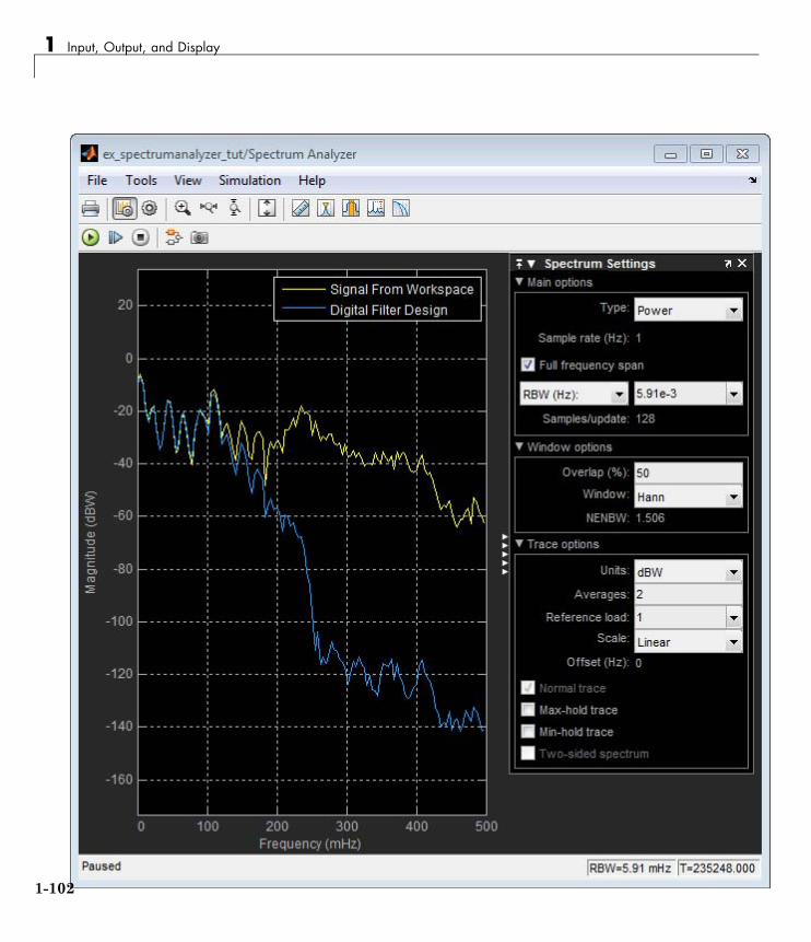
1 Input, Output, and Display
1-102

Display Frequency-Domain Data in Spectrum Analyzer
The power spectrum of the first input signal, from column one, is the yellowline. The power spectrum of the second input signal, from column two, isthe blue line.
1-103

1 Input, Output, and Display
Visualize Central Limit Theorem in Array Plot
In this section...
“Display a Uniform Distribution” on page 1-104
“Display the Sum of Many Uniform Distributions” on page 1-105
“Inspect Your Data by Zooming” on page 1-107
Display a Uniform DistributionThis example shows how to use and configure the dsp.ArrayPlot to visualizethe Central Limit Theorem. This theorem states that the mean of a largenumber of independent random variables with finite mean and varianceexhibits a normal distribution.
First, generate uniformly distributed random variables in MATLAB usingthe rand function. Find their distributions using the hist function. At theMATLAB command line, type:
numsamples = 1e4;numbins = 20;r = rand(numsamples,1);hst = hist(r,numbins);
Create a new Array Plot object.
hap3 = dsp.ArrayPlot;
Configure the properties of the Array Plot object to plot a histogram.
hap3 = dsp.ArrayPlot;hap3.XOffset = 0;hap3.SampleIncrement = 1/numbins;hap3.PlotType = 'Stem';hap3.YLimits = [0, max(hst)+1];
Call the step method to plot the uniform distribution.
step(hap3,hst');
1-104
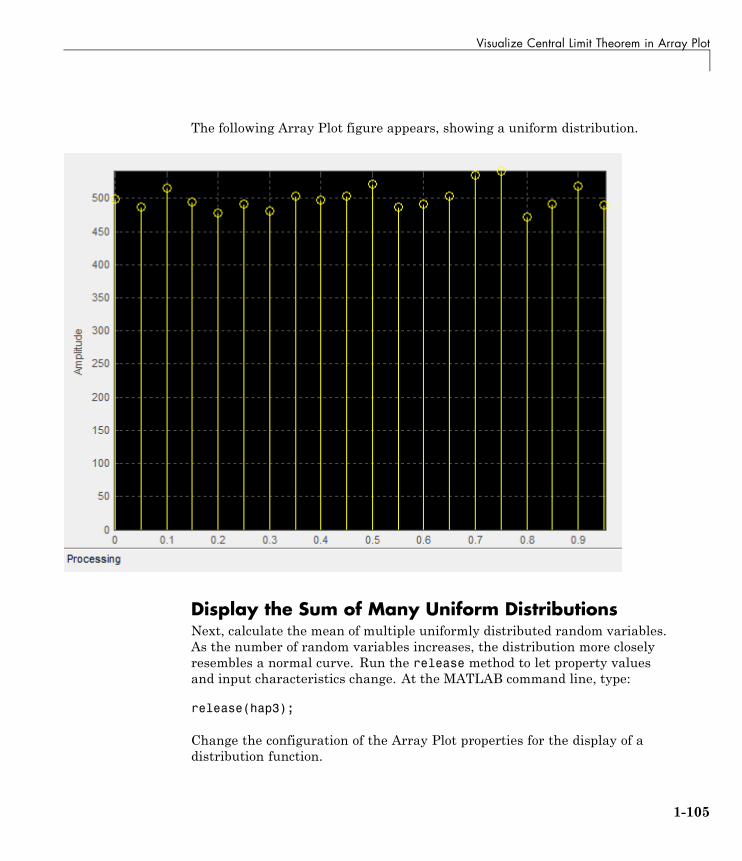
Visualize Central Limit Theorem in Array Plot
The following Array Plot figure appears, showing a uniform distribution.
Display the Sum of Many Uniform DistributionsNext, calculate the mean of multiple uniformly distributed random variables.As the number of random variables increases, the distribution more closelyresembles a normal curve. Run the release method to let property valuesand input characteristics change. At the MATLAB command line, type:
release(hap3);
Change the configuration of the Array Plot properties for the display of adistribution function.
1-105
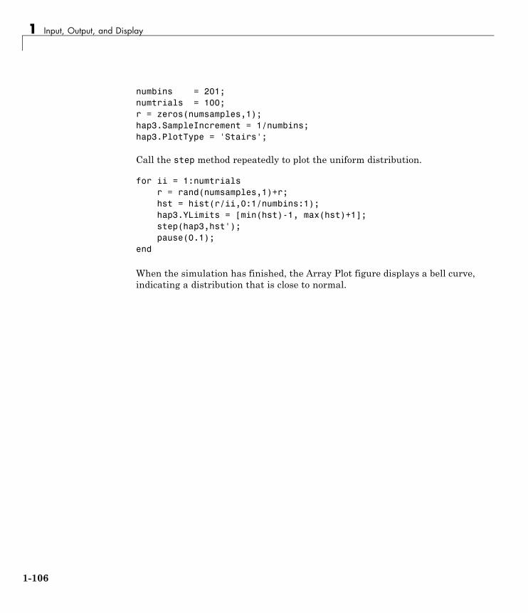
1 Input, Output, and Display
numbins = 201;numtrials = 100;r = zeros(numsamples,1);hap3.SampleIncrement = 1/numbins;hap3.PlotType = 'Stairs';
Call the step method repeatedly to plot the uniform distribution.
for ii = 1:numtrialsr = rand(numsamples,1)+r;hst = hist(r/ii,0:1/numbins:1);hap3.YLimits = [min(hst)-1, max(hst)+1];step(hap3,hst');pause(0.1);
end
When the simulation has finished, the Array Plot figure displays a bell curve,indicating a distribution that is close to normal.
1-106
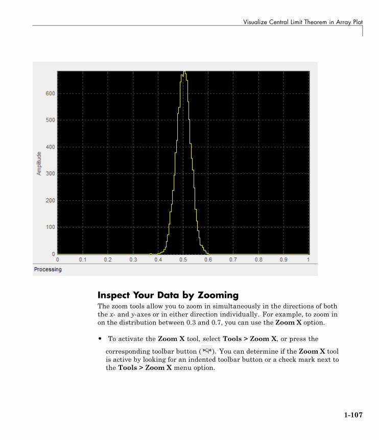
Visualize Central Limit Theorem in Array Plot
Inspect Your Data by ZoomingThe zoom tools allow you to zoom in simultaneously in the directions of boththe x- and y-axes or in either direction individually. For example, to zoom inon the distribution between 0.3 and 0.7, you can use the Zoom X option.
• To activate the Zoom X tool, select Tools > Zoom X, or press the
corresponding toolbar button ( ). You can determine if the Zoom X toolis active by looking for an indented toolbar button or a check mark next tothe Tools > Zoom X menu option.
1-107
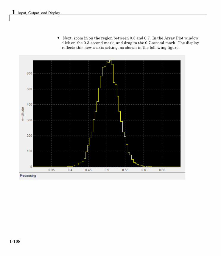
1 Input, Output, and Display
• Next, zoom in on the region between 0.3 and 0.7. In the Array Plot window,click on the 0.3-second mark, and drag to the 0.7-second mark. The displayreflects this new x-axis setting, as shown in the following figure.
1-108

2
Data and SignalManagement
Learn concepts such as sample- and frame-based processing, sample rate,delay and latency.
• “Sample- and Frame-Based Concepts” on page 2-2
• “Inspect Sample and Frame Rates in Simulink” on page 2-8
• “Convert Sample and Frame Rates in Simulink” on page 2-20
• “Buffering and Frame-Based Processing” on page 2-45
• “Delay and Latency” on page 2-61

2 Data and Signal Management
Sample- and Frame-Based Concepts
In this section...
“Sample- and Frame-Based Signals” on page 2-2
“Model Sample- and Frame-Based Signals in MATLAB and Simulink” onpage 2-3
“What Is Sample-Based Processing?” on page 2-4
“What Is Frame-Based Processing?” on page 2-5
Sample- and Frame-Based SignalsSample-based signals are the most basic type of signal and are the easiest toconstruct from a real-world (physical) signal. You can create a sample-basedsignal by sampling a physical signal at a given sample rate, and outputtingeach individual sample as it is received. In general, most Digital-to-Analogconverters output sample-based signals.
You can create frame-based signals from sample-based signals. When youbuffer a batch of N samples, you create a frame of data. You can then outputsequential frames of data at a rate that is 1/N times the sample rate of theoriginal sample-based signal. The rate at which you output the frames of datais also known as the frame rate of the signal.
Frame-based data is a common format in real-time systems. Data acquisitionhardware often operates by accumulating a large number of signal samples ata high rate. The hardware then propagates those samples to the real-timesystem as a block of data. Doing so maximizes the efficiency of the systemby distributing the fixed process overhead across many samples. The fasterdata acquisition is suspended by slower interrupt processes after each frameis acquired, rather than after each individual sample. See “Benefits ofFrame-Based Processing” on page 2-6 for more information.
2-2

Sample- and Frame-Based Concepts
DSP System ToolboxSource Blocks
CreateSample-BasedSignals
Create Frame-BasedSignals
Chirp X X
Constant X X
Constant DiagonalMatrix
X
Discrete Impulse X X
DSP Constant (Obsolete) X
From Audio Device X X
From Multimedia File X X
Identity Matrix X
MIDI Controls X
Multiphase Clock X X
N-Sample Enable X X
Random Source X
Signal From Workspace X X
Sine Wave X X
UDP Receive X
Model Sample- and Frame-Based Signals in MATLABand SimulinkWhen you process signals using DSP System Toolbox software, you can doso in either a sample- or frame-based manner. When you are working withblocks in Simulink, you can specify, on a block-by-block basis, which typeof processing the block performs. In most cases, you specify the processingmode by setting the Input processing parameter. Alternatively, whenyou are using System objects in MATLAB, you specify the processing modeusing the FrameBasedProcessing property. The following table shows thecommon parameter settings you can use to perform sample- and frame-basedprocessing in MATLAB and Simulink.
2-3

2 Data and Signal Management
Sample-BasedProcessing
Frame-BasedProcessing
MATLAB — Systemobjects
FrameBasedProcessing= False
FrameBasedProcessing= True
Simulink — Blocks Input processing= Elements aschannels (samplebased)
Input processing =Columns as channels(frame based)
Set the FrameBasedProcessing Property of a System objectAll System objects support sample-based processing and some System objectssupport both sample- and frame-based processing. To specify how your Systemobject™ should process input data, you set the FrameBasedProcessingproperty. The property has a default value of true, which enablesframe-based processing. To specify sample-based processing, set theFrameBasedProcessing property to false.
What Is Sample-Based Processing?In sample-based processing, blocks process signals one sample at a time. Eachelement of the input signal represents one sample in a distinct channel. Forexample, from a sample-based processing perspective, the following 3-by-2matrix contains the first sample in each of six independent channels.
When you configure a block to perform sample-based processing, the blockinterprets scalar input as a single-channel signal. Similarly, the blockinterprets an M-by-N matrix as multichannel signal with M*N independentchannels. For example, in sample-based processing, blocks interpret thefollowing sequence of 3-by-2 matrices as a six-channel signal.
2-4
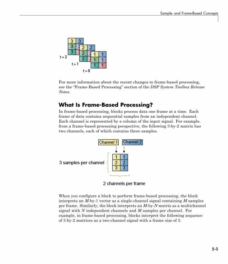
Sample- and Frame-Based Concepts
For more information about the recent changes to frame-based processing,see the “Frame-Based Processing” section of the DSP System Toolbox ReleaseNotes.
What Is Frame-Based Processing?In frame-based processing, blocks process data one frame at a time. Eachframe of data contains sequential samples from an independent channel.Each channel is represented by a column of the input signal. For example,from a frame-based processing perspective, the following 3-by-2 matrix hastwo channels, each of which contains three samples.
When you configure a block to perform frame-based processing, the blockinterprets an M-by-1 vector as a single-channel signal containing M samplesper frame. Similarly, the block interprets anM-by-Nmatrix as a multichannelsignal with N independent channels and M samples per channel. Forexample, in frame-based processing, blocks interpret the following sequenceof 3-by-2 matrices as a two-channel signal with a frame size of 3.
2-5

2 Data and Signal Management
Using frame-based processing is advantageous for many signal processingapplications because you can process multiple samples at once. By bufferingyour data into frames and processing multisample frames of data, you canoften improve the computational time of your signal processing algorithms.To perform frame-based processing, you must have a DSP System Toolboxlicense.
For more information about the recent changes to frame-based processing,see the “Frame-Based Processing” section of the DSP System Toolbox ReleaseNotes.
Benefits of Frame-Based ProcessingFrame-based processing is an established method of accelerating bothreal-time systems and model simulations.
Accelerate Real-Time Systems. Frame-based data is a common format inreal-time systems. Data acquisition hardware often operates by accumulatinga large number of signal samples at a high rate, and then propagating thosesamples to the real-time system as a block of data. This type of propagationmaximizes the efficiency of the system by distributing the fixed processoverhead across many samples; the faster data acquisition is suspended byslower interrupt processes after each frame is acquired, rather than aftereach individual sample is acquired.
The following figure illustrates how frame-based processing increasesthroughput. The thin blocks each represent the time elapsed during
2-6
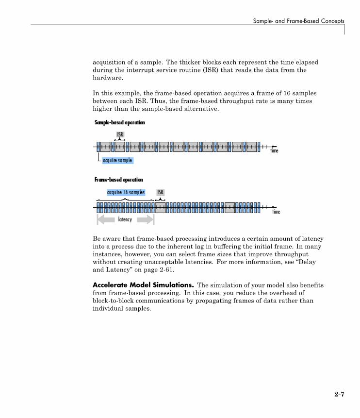
Sample- and Frame-Based Concepts
acquisition of a sample. The thicker blocks each represent the time elapsedduring the interrupt service routine (ISR) that reads the data from thehardware.
In this example, the frame-based operation acquires a frame of 16 samplesbetween each ISR. Thus, the frame-based throughput rate is many timeshigher than the sample-based alternative.
Be aware that frame-based processing introduces a certain amount of latencyinto a process due to the inherent lag in buffering the initial frame. In manyinstances, however, you can select frame sizes that improve throughputwithout creating unacceptable latencies. For more information, see “Delayand Latency” on page 2-61.
Accelerate Model Simulations. The simulation of your model also benefitsfrom frame-based processing. In this case, you reduce the overhead ofblock-to-block communications by propagating frames of data rather thanindividual samples.
2-7
2 Data and Signal Management
Inspect Sample and Frame Rates in Simulink
Note Starting in R2010b, many DSP System Toolbox blocks received a newparameter to control whether they perform sample- or frame-based processing.The following content has not been updated to reflect this change. For moreinformation, see the “Frame-Based Processing” section of the Release Notes.
In this section...
“Sample Rate and Frame Rate Concepts” on page 2-8
“Inspect Sample-Based Signals Using Probe Block” on page 2-10
“Inspect Frame-Based Signals Using Probe Block” on page 2-12
“Inspect Sample-Based Signals Using Color Coding” on page 2-15
“Inspect Frame-Based Signals Using Color Coding” on page 2-16
Sample Rate and Frame Rate ConceptsSample rates and frame rates are important issues in most signal processingmodels. This is especially true with systems that incorporate rate conversions.Fortunately, in most cases when you build a Simulink model, you only needto set sample rates for the source blocks. Simulink automatically computesthe appropriate sample rates for the blocks that are connected to the sourceblocks. Nevertheless, it is important to become familiar with the sample rateand frame rate concepts as they apply to Simulink models.
The input frame period (Tfi) of a frame-based signal is the time intervalbetween consecutive vector or matrix inputs to a block. Similarly, theoutput frame period (Tfo) is the time interval at which the block updates theframe-based vector or matrix value at the output port.
In contrast, the sample period, Ts, is the time interval between individualsamples in a frame, this value is shorter than the frame period when theframe size is greater than 1. The sample period of a frame-based signal is thequotient of the frame period and the frame size, M:
2-8
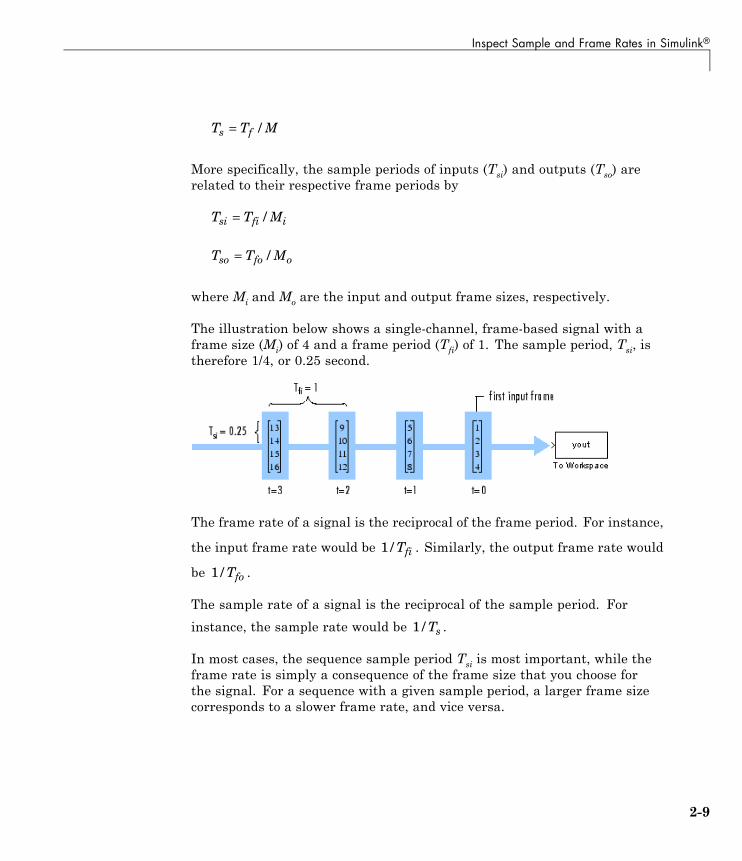
Inspect Sample and Frame Rates in Simulink®
T T Ms f= /
More specifically, the sample periods of inputs (Tsi) and outputs (Tso) arerelated to their respective frame periods by
T T Msi fi i= /
T T Mso fo o= /
where Mi and Mo are the input and output frame sizes, respectively.
The illustration below shows a single-channel, frame-based signal with aframe size (Mi) of 4 and a frame period (Tfi) of 1. The sample period, Tsi, istherefore 1/4, or 0.25 second.
The frame rate of a signal is the reciprocal of the frame period. For instance,
the input frame rate would be 1 / Tfi . Similarly, the output frame rate would
be 1 / Tfo .
The sample rate of a signal is the reciprocal of the sample period. For
instance, the sample rate would be 1 / Ts .
In most cases, the sequence sample period Tsi is most important, while theframe rate is simply a consequence of the frame size that you choose forthe signal. For a sequence with a given sample period, a larger frame sizecorresponds to a slower frame rate, and vice versa.
2-9

2 Data and Signal Management
Inspect Sample-Based Signals Using Probe BlockYou can use the Probe block to display the sample period of a sample-basedsignal. For sample-based signals, the Probe block displays the label Ts, thesample period of the sequence, followed by a two-element vector. The leftelement is the period of the signal being measured. The right element is thesignal’s sample time offset, which is usually 0.
Note Simulink offers the ability to shift the sample time of a signal byan arbitrary value, which is equivalent to shifting the signal’s phase by afractional sample period. However, sample-time offsets are rarely used insignal processing systems, and DSP System Toolbox blocks do not supportthem.
In this example, you use the Probe block to display the sample period of asample-based signal:
1 At the MATLAB command prompt, type ex_probe_tut1.
The Probe Example 1 model opens.
2-10

Inspect Sample and Frame Rates in Simulink®
2 Run the model.
The figure below illustrates how the Probe blocks display the sample periodof the signal before and after each upsample operation.
2-11
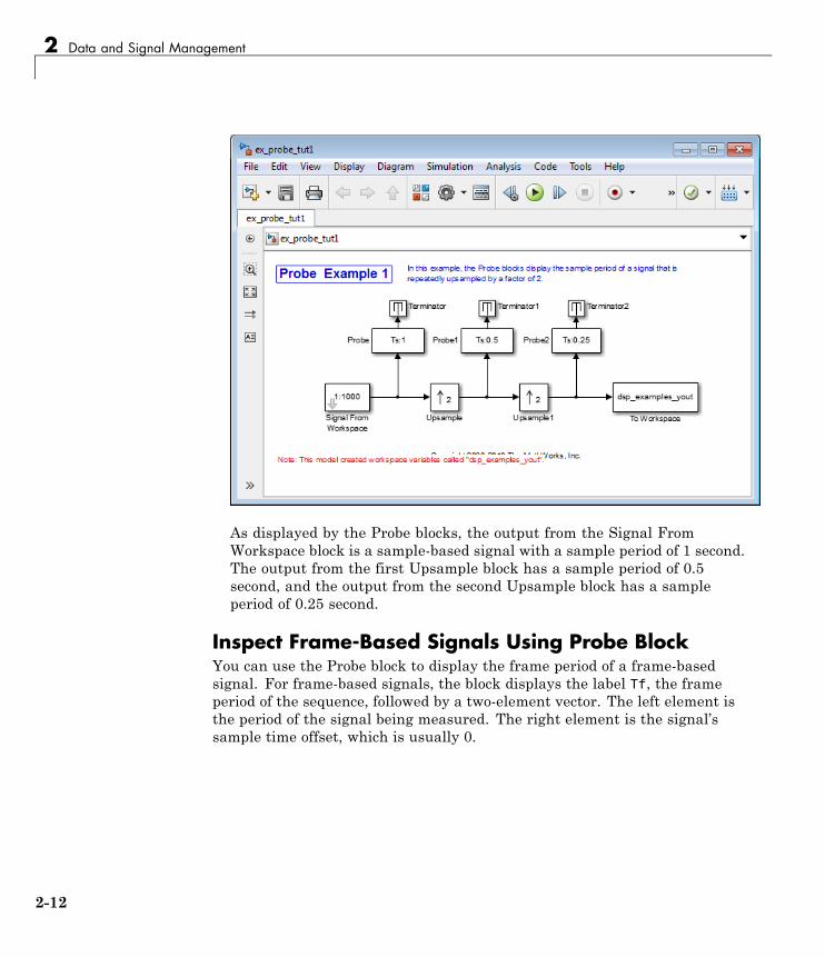
2 Data and Signal Management
As displayed by the Probe blocks, the output from the Signal FromWorkspace block is a sample-based signal with a sample period of 1 second.The output from the first Upsample block has a sample period of 0.5second, and the output from the second Upsample block has a sampleperiod of 0.25 second.
Inspect Frame-Based Signals Using Probe BlockYou can use the Probe block to display the frame period of a frame-basedsignal. For frame-based signals, the block displays the label Tf, the frameperiod of the sequence, followed by a two-element vector. The left element isthe period of the signal being measured. The right element is the signal’ssample time offset, which is usually 0.
2-12
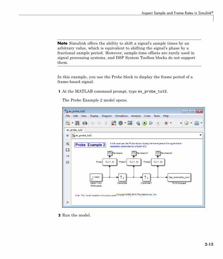
Inspect Sample and Frame Rates in Simulink®
Note Simulink offers the ability to shift a signal’s sample times by anarbitrary value, which is equivalent to shifting the signal’s phase by afractional sample period. However, sample-time offsets are rarely used insignal processing systems, and DSP System Toolbox blocks do not supportthem.
In this example, you use the Probe block to display the frame period of aframe-based signal:
1 At the MATLAB command prompt, type ex_probe_tut2.
The Probe Example 2 model opens.
2 Run the model.
2-13

2 Data and Signal Management
The figure below illustrates how the Probe blocks display the frame periodof the signal before and after each upsample operation.
As displayed by the Probe blocks, the output from the Signal FromWorkspace block is a frame-based signal with a frame period of 16 seconds.The output from the first Upsample block has a frame period of 8 seconds,and the output from the second Upsample block has a sample period of 4seconds.
Note that the sample rate conversion is implemented through a change in theframe period rather than the frame size.
2-14

Inspect Sample and Frame Rates in Simulink®
Inspect Sample-Based Signals Using Color CodingIn the following example, you use sample time color coding to view the samplerate of a sample-based signal:
1 At the MATLAB command prompt, type ex_color_tut1.
The Sample Time Color Example 1 model opens.
2 From the Display menu, point to Sample Time, and select Colors.
This selection turns on sample time color coding. Simulink now assignseach sample rate a different color.
3 Run the model.
The model should now look similar to the following figure:
2-15
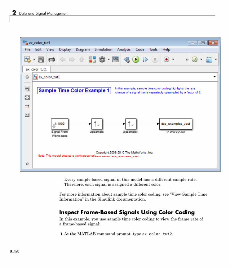
2 Data and Signal Management
Every sample-based signal in this model has a different sample rate.Therefore, each signal is assigned a different color.
For more information about sample time color coding, see “View Sample TimeInformation” in the Simulink documentation.
Inspect Frame-Based Signals Using Color CodingIn this example, you use sample time color coding to view the frame rate ofa frame-based signal:
1 At the MATLAB command prompt, type ex_color_tut2.
2-16
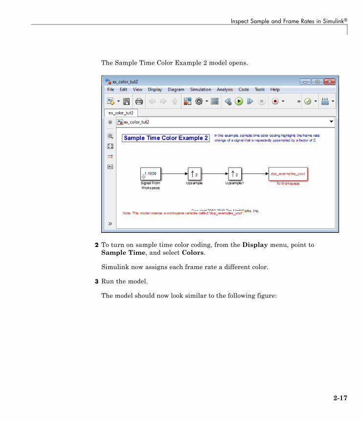
Inspect Sample and Frame Rates in Simulink®
The Sample Time Color Example 2 model opens.
2 To turn on sample time color coding, from the Display menu, point toSample Time, and select Colors.
Simulink now assigns each frame rate a different color.
3 Run the model.
The model should now look similar to the following figure:
2-17

2 Data and Signal Management
Because the Rate options parameter in the Upsample blocks is setto Allow multirate processing, each Upsample block changes theframe rate. Therefore, each frame-based signal in the model is assigneda different color.
4 Double-click on each Upsample block and change the Rate optionsparameter to Enforce single-rate processing.
5 Run the model.
Every signal is coded with the same color. Therefore, every signal in themodel now has the same frame rate.
2-18

Inspect Sample and Frame Rates in Simulink®
For more information about sample tim color coding, see “View Sample TimeInformation” in the Simulink documentation.
2-19
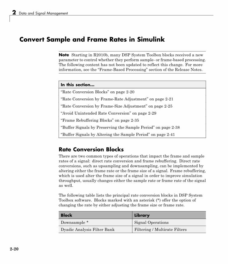
2 Data and Signal Management
Convert Sample and Frame Rates in Simulink
Note Starting in R2010b, many DSP System Toolbox blocks received a newparameter to control whether they perform sample- or frame-based processing.The following content has not been updated to reflect this change. For moreinformation, see the “Frame-Based Processing” section of the Release Notes.
In this section...
“Rate Conversion Blocks” on page 2-20
“Rate Conversion by Frame-Rate Adjustment” on page 2-21
“Rate Conversion by Frame-Size Adjustment” on page 2-25
“Avoid Unintended Rate Conversion” on page 2-29
“Frame Rebuffering Blocks” on page 2-35
“Buffer Signals by Preserving the Sample Period” on page 2-38
“Buffer Signals by Altering the Sample Period” on page 2-41
Rate Conversion BlocksThere are two common types of operations that impact the frame and samplerates of a signal: direct rate conversion and frame rebuffering. Direct rateconversions, such as upsampling and downsampling, can be implemented byaltering either the frame rate or the frame size of a signal. Frame rebuffering,which is used alter the frame size of a signal in order to improve simulationthroughput, usually changes either the sample rate or frame rate of the signalas well.
The following table lists the principal rate conversion blocks in DSP SystemToolbox software. Blocks marked with an asterisk (*) offer the option ofchanging the rate by either adjusting the frame size or frame rate.
Block Library
Downsample * Signal Operations
Dyadic Analysis Filter Bank Filtering / Multirate Filters
2-20
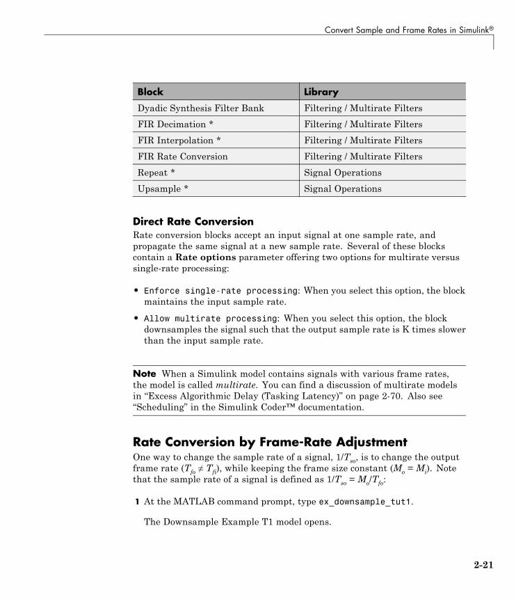
Convert Sample and Frame Rates in Simulink®
Block Library
Dyadic Synthesis Filter Bank Filtering / Multirate Filters
FIR Decimation * Filtering / Multirate Filters
FIR Interpolation * Filtering / Multirate Filters
FIR Rate Conversion Filtering / Multirate Filters
Repeat * Signal Operations
Upsample * Signal Operations
Direct Rate ConversionRate conversion blocks accept an input signal at one sample rate, andpropagate the same signal at a new sample rate. Several of these blockscontain a Rate options parameter offering two options for multirate versussingle-rate processing:
• Enforce single-rate processing: When you select this option, the blockmaintains the input sample rate.
• Allow multirate processing: When you select this option, the blockdownsamples the signal such that the output sample rate is K times slowerthan the input sample rate.
Note When a Simulink model contains signals with various frame rates,the model is called multirate. You can find a discussion of multirate modelsin “Excess Algorithmic Delay (Tasking Latency)” on page 2-70. Also see“Scheduling” in the Simulink Coder™ documentation.
Rate Conversion by Frame-Rate AdjustmentOne way to change the sample rate of a signal, 1/Tso, is to change the outputframe rate (Tfo ≠ Tfi), while keeping the frame size constant (Mo = Mi). Notethat the sample rate of a signal is defined as 1/Tso = Mo/Tfo:
1 At the MATLAB command prompt, type ex_downsample_tut1.
The Downsample Example T1 model opens.
2-21

2 Data and Signal Management
2 From the Display menu, point to Signals & Ports, and select SignalDimensions.
When you run the model, the dimensions of the signals appear next to thelines connecting the blocks.
3 Double-click the Signal From Workspace block. The Source BlockParameters: Signal From Workspace dialog box opens.
4 Set the block parameters as follows:
• Sample time = 0.125
2-22

Convert Sample and Frame Rates in Simulink®
• Samples per frame = 8
Based on these parameters, the Signal From Workspace block outputs aframe-based signal with a sample period of 0.125 second and a frame sizeof 8.
5 Save these parameters and close the dialog box by clicking OK.
6 Double-click the Downsample block. The Function Block Parameters:Downsample dialog box opens.
7 Set the Rate options parameter to Allow multirate processing, andthen click OK.
The Downsample block is configured to downsample the signal by changingthe frame rate rather than the frame size.
8 Run the model.
After the simulation, the model should look similar to the following figure.
2-23
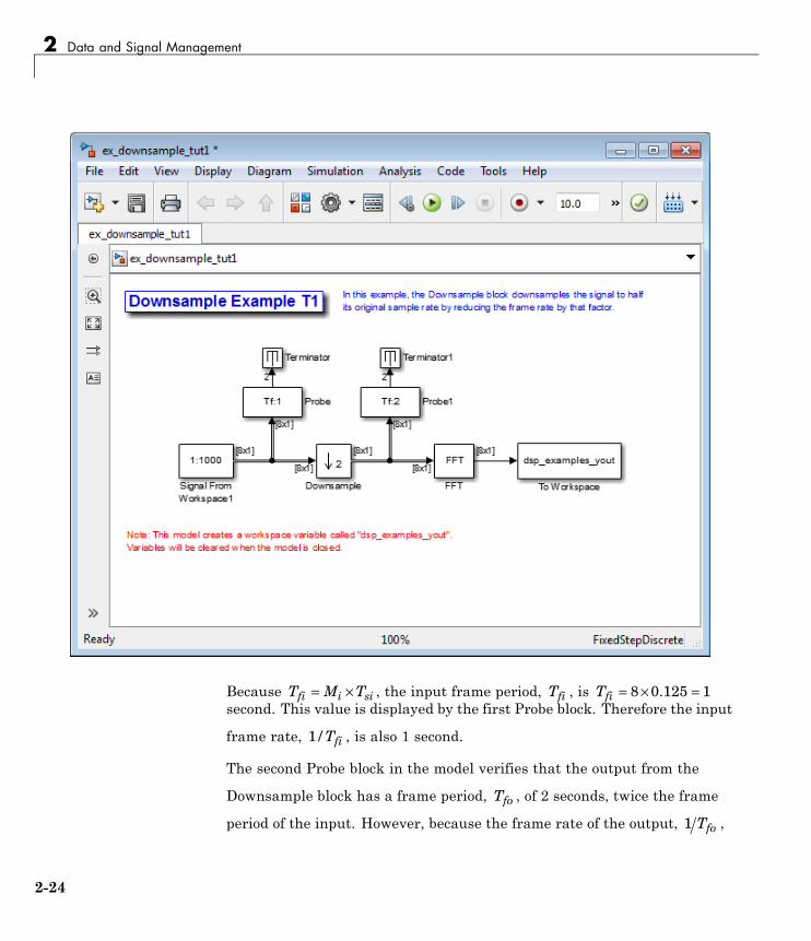
2 Data and Signal Management
Because T M Tfi i si= × , the input frame period, Tfi , is Tfi = × =8 0 125 1.second. This value is displayed by the first Probe block. Therefore the input
frame rate, 1 / Tfi , is also 1 second.
The second Probe block in the model verifies that the output from the
Downsample block has a frame period, Tfo , of 2 seconds, twice the frame
period of the input. However, because the frame rate of the output, 1 Tfo ,
2-24

Convert Sample and Frame Rates in Simulink®
is 0.5 second, the Downsample block actually downsampled the originalsignal to half its original rate. As a result, the output sample period,
T T Mso fo o= / , is doubled to 0.25 second without any change to the framesize. The signal dimensions in the model confirm that the frame size didnot change.
Rate Conversion by Frame-Size AdjustmentOne way to change the sample rate of a signal is by changing the frame size(that is Mo ≠ Mi), but keep the frame rate constant (Tfo = Tfi). Note that thesample rate of a signal is defined as 1/Tso = Mo/Tfo:
1 At the MATLAB command prompt, type ex_downsample_tut2.
The Downsample Example T2 model opens.
2-25

2 Data and Signal Management
2 From the Display menu, point to Signals & Ports, and select SignalDimensions.
When you run the model, the dimensions of the signals appear next to thelines connecting the blocks.
3 Double-click the Signal From Workspace block. The Source BlockParameters: Signal From Workspace dialog box opens.
4 Set the block parameters as follows:
• Sample time = 0.125
2-26

Convert Sample and Frame Rates in Simulink®
• Samples per frame = 8
Based on these parameters, the Signal From Workspace block outputs aframe-based signal with a sample period of 0.125 second and a frame sizeof 8.
5 Save these parameters and close the dialog box by clicking OK.
6 Double-click the Downsample block. The Function Block Parameters:Downsample dialog box opens.
7 Set the Rate options parameter to Enforce single-rate processing,and then click OK.
The Downsample block is configured to downsample the signal by changingthe frame size rather than the frame rate.
8 Run the model.
After the simulation, the model should look similar to the following figure.
2-27

2 Data and Signal Management
Because T M Tfi i si= × , the input frame period, Tfi , is Tfi = × =8 0 125 1.second. This value is displayed by the first Probe block. Therefore the input
frame rate, 1 / Tfi , is also 1 second.
The Downsample block downsampled the input signal to half its originalframe size. The signal dimensions of the output of the Downsampleblock confirm that the downsampled output has a frame size of 4, halfthe frame size of the input. As a result, the sample period of the output,
2-28
Convert Sample and Frame Rates in Simulink®
T T Mso fo o= / , now has a sample period of 0.25 second. This process
occurred without any change to the frame rate (T Tfi fo= ).
Avoid Unintended Rate ConversionIt is important to be aware of where rate conversions occur in a model. In afew cases, unintentional rate conversions can produce misleading results:
1 At the MATLAB command prompt, type ex_vectorscope_tut1.
The Vector Scope Example model opens.
2 Double-click the upper Sine Wave block. The Source Block Parameters:Sine Wave dialog box opens.
3 Set the block parameters as follows:
• Frequency (Hz) = 1
• Sample time = 0.1
• Samples per frame = 128
Based on the Sample time and the Samples per frame parameters,the Sine Wave outputs a sinusoid with a frame period of 128*0.1 or 12.8seconds.
4 Save these parameters and close the dialog box by clicking OK.
5 Double-click the lower Sine Wave block.
6 Set the block parameters as follows, and then click OK:
• Frequency (Hz) = 2
• Sample time = 0.1
• Samples per frame = 128
Based on the Sample time and the Samples per frame parameters,the Sine Wave outputs a sinusoid with a frame period of 128*0.1 or 12.8seconds.
2-29

2 Data and Signal Management
7 Double-click the Magnitude FFT block. The Function Block Parameters:Magnitude FFT dialog box opens.
8 Select the Inherit FFT length from input dimensions check box, andthen click OK.
This setting instructs the block to use the input frame size (128) as the FFTlength (which is also the output size).
9 Double-click the Vector Scope block. The Sink Block Parameters:Vector Scope dialog box opens.
10 Set the block parameters as follows, and then click OK:
• Click the Scope Properties tab.
• Input domain = Frequency
• Click the Axis Properties tab.
• Minimum Y-limit = -10
• Maximum Y-limit = 40
11 Run the model.
The model should now look similar to the following figure. Note that thesignal leaving the Magnitude FFT block is 128-by-1.
2-30

Convert Sample and Frame Rates in Simulink®
The Vector Scope window displays the magnitude FFT of a signalcomposed of two sine waves, with frequencies of 1 Hz and 2 Hz.
2-31

2 Data and Signal Management
The Vector Scope block uses the input frame size (128) and period (12.8) todeduce the original signal’s sample period (0.1), which allows it to correctlydisplay the peaks at 1 Hz and 2 Hz.
12 Double-click the Magnitude FFT block. The Function Block Parameters:Magnitude FFT dialog box opens.
13 Set the block parameters as follows:
• Clear the Inherit FFT length from input dimensions check box.
• Set the FFT length parameter to 256.
Based on these parameters, the Magnitude FFT block zero-pads thelength-128 input frame to a length of 256 before performing the FFT.
2-32

Convert Sample and Frame Rates in Simulink®
14 Run the model.
The model should now look similar to the following figure. Note that thesignal leaving the Magnitude FFT block is 256-by-1.
The Vector Scope window displays the magnitude FFT of a signalcomposed of two sine waves, with frequencies of 2 Hz and 4 Hz.
2-33
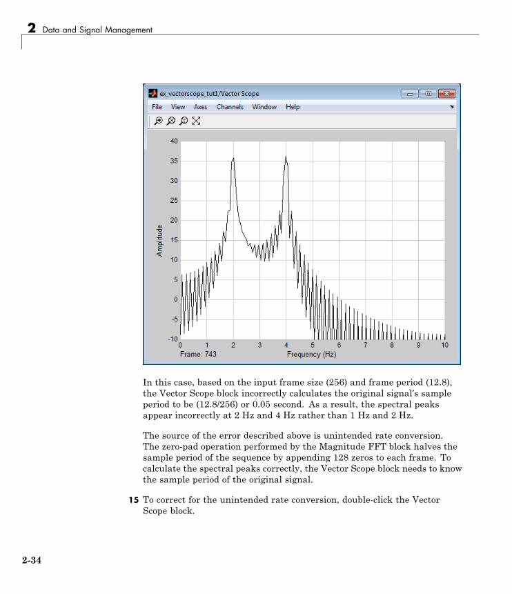
2 Data and Signal Management
In this case, based on the input frame size (256) and frame period (12.8),the Vector Scope block incorrectly calculates the original signal’s sampleperiod to be (12.8/256) or 0.05 second. As a result, the spectral peaksappear incorrectly at 2 Hz and 4 Hz rather than 1 Hz and 2 Hz.
The source of the error described above is unintended rate conversion.The zero-pad operation performed by the Magnitude FFT block halves thesample period of the sequence by appending 128 zeros to each frame. Tocalculate the spectral peaks correctly, the Vector Scope block needs to knowthe sample period of the original signal.
15 To correct for the unintended rate conversion, double-click the VectorScope block.
2-34

Convert Sample and Frame Rates in Simulink®
16 Set the block parameters as follows:
• Click the Axis Properties tab.
• Clear the Inherit sample time from input check box.
• Set the Sample time of original time series parameter to the actualsample period of 0.1.
17 Run the model.
The Vector Scope block now accurately plots the spectral peaks at 1 Hzand 2 Hz.
In general, when you zero-pad or overlap buffers, you are changing the sampleperiod of the signal. If you keep this in mind, you can anticipate and correctproblems such as unintended rate conversion.
Frame Rebuffering BlocksThere are two common types of operations that impact the frame and samplerates of a signal: direct rate conversion and frame rebuffering. Direct rateconversions, such as upsampling and downsampling, can be implemented byaltering either the frame rate or the frame size of a signal. Frame rebuffering,which is used alter the frame size of a signal in order to improve simulationthroughput, usually changes either the sample rate or frame rate of the signalas well.
Sometimes you might need to rebuffer a signal to a new frame size at somepoint in a model. For example, your data acquisition hardware may internallybuffer the sampled signal to a frame size that is not optimal for the signalprocessing algorithm in the model. In this case, you would want to rebufferthe signal to a frame size more appropriate for the intended operationswithout introducing any change to the data or sample rate.
The following table lists the principal DSP System Toolbox buffering blocks.
Block Library
Buffer Signal Management/ Buffers
Delay Line Signal Management/ Buffers
2-35
2 Data and Signal Management
Block Library
Unbuffer Signal Management/ Buffers
Variable Selector Signal Management/ Indexing
Blocks for Frame Rebuffering with Preservation of the SignalBuffering operations provide another mechanism for rate changes in signalprocessing models. The purpose of many buffering operations is to adjustthe frame size of the signal, M, without altering the signal’s sample rate Ts.This usually results in a change to the signal’s frame rate, Tf, according tothe following equation:
T MTf s=
However, the equation above is only true if no samples are added or deletedfrom the original signal. Therefore, the equation above does not apply tobuffering operations that generate overlapping frames, that only partiallyunbuffer frames, or that alter the data sequence by adding or deletingsamples.
There are two blocks in the Buffers library that can be used to change asignal’s frame size without altering the signal itself:
• Buffer — redistributes signal samples to a larger or smaller frame size
• Unbuffer — unbuffers a frame-based signal to a sample-based signal(frame size = 1)
The Buffer block preserves the signal’s data and sample period only when itsBuffer overlap parameter is set to 0. The output frame period, Tfo, is
TM T
Mfoo fi
i=
where Tfi is the input frame period, Mi is the input frame size, and Mo isthe output frame size specified by the Output buffer size (per channel)parameter.
2-36
Convert Sample and Frame Rates in Simulink®
The Unbuffer block unbuffers a frame-based signal to its sample-basedequivalent, and always preserves the signal’s data and sample period
T T Mso fi i= /
where Tfi and Mi are the period and size, respectively, of the frame-basedinput.
Both the Buffer and Unbuffer blocks preserve the sample period of thesequence in the conversion (Tso = Tsi).
Blocks for Frame Rebuffering with Alteration of the SignalSome forms of buffering alter the signal’s data or sample period in addition toadjusting the frame size. This type of buffering is desirable when you want tocreate sliding windows by overlapping consecutive frames of a signal, or selecta subset of samples from each input frame for processing.
The blocks that alter a signal while adjusting its frame size are listed below.In this list, Tsi is the input sequence sample period, and Tfi and Tfo are theinput and output frame periods, respectively:
• The Buffer block adds duplicate samples to a sequence when the Bufferoverlap parameter, L, is set to a nonzero value. The output frame periodis related to the input sample period by
T M L Tfo o si= −( )
where Mo is the output frame size specified by the Output buffer size(per channel) parameter. As a result, the new output sample period is
TM L T
Msoo si
o=
−( )
• The Delay Line block adds duplicate samples to the sequence when theDelay line size parameter, Mo, is greater than 1. The output and inputframe periods are the same, Tfo = Tfi = Tsi, and the new output sampleperiod is
2-37

2 Data and Signal Management
TTMso
si
o=
• The Variable Selector block can remove, add, and/or rearrange samples inthe input frame when Select is set to Rows. The output and input frameperiods are the same, Tfo = Tfi, and the new output sample period is
TM TMsoi si
o=
where Mo is the length of the block’s output, determined by the Elementsvector.
In all of these cases, the sample period of the output sequence is not equal tothe sample period of the input sequence.
Buffer Signals by Preserving the Sample PeriodIn the following example, a signal with a sample period of 0.125 second isrebuffered from a frame size of 8 to a frame size of 16. This rebufferingprocess doubles the frame period from 1 to 2 seconds, but does not change thesample period of the signal (Tso = Tsi = 0.125). The process also does not add ordelete samples from the original signal:
1 At the MATLAB command prompt, type ex_buffer_tut1.
The Buffer Example T1 model opens.
2-38

Convert Sample and Frame Rates in Simulink®
2 Double-click the Signal From Workspace block. The Source BlockParameters: Signal From Workspace dialog box opens.
3 Set the parameters as follows:
• Signal = 1:1000
• Sample time = 0.125
• Samples per frame = 8
• Form output after final data value = Setting to zero
Based on these parameters, the Signal from Workspace block outputs aframe-based signal with a sample period of 0.125 second. Each outputframe contains eight samples.
2-39

2 Data and Signal Management
4 Save these parameters and close the dialog box by clicking OK.
5 Double-click the Buffer block. The Function Block Parameters: Bufferdialog box opens.
6 Set the parameters as follows, and then click OK:
• Output buffer size (per channel) = 16
• Buffer overlap = 0
• Initial conditions = 0
Based on these parameters, the Buffer block rebuffers the signal from aframe size of 8 to a frame size of 16.
7 Run the model.
The following figure shows the model after simulation.
2-40

Convert Sample and Frame Rates in Simulink®
Note that the input to the Buffer block has a frame size of 8 and the outputof the block has a frame size of 16. As shown by the Probe blocks, therebuffering process doubles the frame period from 1 to 2 seconds.
Buffer Signals by Altering the Sample PeriodSome forms of buffering alter the signal’s data or sample period in addition toadjusting the frame size. In the following example, a signal with a sampleperiod of 0.125 second is rebuffered from a frame size of 8 to a frame sizeof 16 with a buffer overlap of 4:
1 At the MATLAB command prompt, type ex_buffer_tut2.
The Buffer Example T2 model opens.
2-41

2 Data and Signal Management
2 Double-click the Signal From Workspace block. The Source BlockParameters: Signal From Workspace dialog box opens.
3 Set the parameters as follows:
• Signal = 1:1000
• Sample time = 0.125
• Samples per frame = 8
• Form output after final data value = Setting to zero
Based on these parameters, the Signal from Workspace block outputs aframe-based signal with a sample period of 0.125 second. Each outputframe contains eight samples.
2-42

Convert Sample and Frame Rates in Simulink®
4 Save these parameters and close the dialog box by clicking OK.
5 Double-click the Buffer block. The Function Block Parameters: Bufferdialog box opens.
6 Set the parameters as follows, and then click OK:
• Output buffer size (per channel) = 16
• Buffer overlap = 4
• Initial conditions = 0
Based on these parameters, the Buffer block rebuffers the signal from aframe size of 8 to a frame size of 16. Also, after the initial output, the firstfour samples of each output frame are made up of the last four samplesfrom the previous output frame.
7 Run the model.
The following figure shows the model after the simulation has stopped.
2-43

2 Data and Signal Management
Note that the input to the Buffer block has a frame size of 8 and the outputof the block has a frame size of 16. The relation for the output frame periodfor the Buffer block is
T M L Tfo o si= −( )
Tfo is (16-4)*0.125, or 1.5 seconds, as confirmed by the second Probe block.The sample period of the signal at the output of the Buffer block is no
longer 0.125 second. It is now T T Mso fo o= = =/ . / .1 5 16 0 0938 second.Thus, both the signal’s data and the signal’s sample period have beenaltered by the buffering operation.
2-44
Buffering and Frame-Based Processing
Buffering and Frame-Based Processing
Note Starting in R2010b, many DSP System Toolbox blocks received a newparameter to control whether they perform sample- or frame-based processing.The following content has not been updated to reflect this change. For moreinformation, see the “Frame-Based Processing” section of the Release Notes.
In this section...
“Frame Status” on page 2-45
“Buffer Sample-Based Signals into Frame-Based Signals” on page 2-45
“Buffer Sample-Based Signals into Frame-Based Signals with Overlap”on page 2-49
“Buffer Frame-Based Signals into Other Frame-Based Signals” on page 2-53
“Buffer Delay and Initial Conditions” on page 2-56
“Unbuffer Frame-Based Signals into Sample-Based Signals” on page 2-57
Frame StatusThe frame status of a signal refers to whether the signal is sample based orframe based. In a Simulink model, the frame status is symbolized by a singleline ,→, for a sample-based signal and a double line, for a frame-basedsignal. One way to convert a sample-based signal to a frame-based signalis by using the Buffer block. You can convert a frame-based signal to asample-based signal using the Unbuffer block. To change the frame status ofa signal without performing a buffering operation, use the Frame Conversionblock in the Signal Attributes library.
Buffer Sample-Based Signals into Frame-BasedSignalsMultichannel sample-based and frame-based signals can be buffered intomultichannel frame-based signals using the Buffer block.
2-45
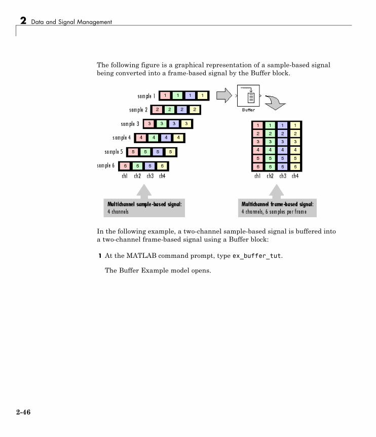
2 Data and Signal Management
The following figure is a graphical representation of a sample-based signalbeing converted into a frame-based signal by the Buffer block.
In the following example, a two-channel sample-based signal is buffered intoa two-channel frame-based signal using a Buffer block:
1 At the MATLAB command prompt, type ex_buffer_tut.
The Buffer Example model opens.
2-46
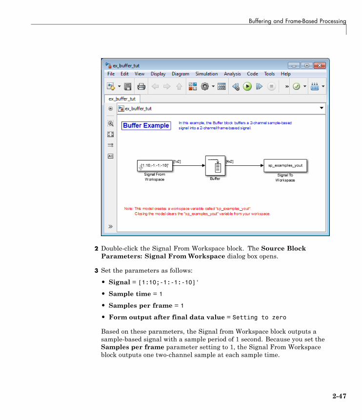
Buffering and Frame-Based Processing
2 Double-click the Signal From Workspace block. The Source BlockParameters: Signal From Workspace dialog box opens.
3 Set the parameters as follows:
• Signal = [1:10;-1:-1:-10]'
• Sample time = 1
• Samples per frame = 1
• Form output after final data value = Setting to zero
Based on these parameters, the Signal from Workspace block outputs asample-based signal with a sample period of 1 second. Because you set theSamples per frame parameter setting to 1, the Signal From Workspaceblock outputs one two-channel sample at each sample time.
2-47

2 Data and Signal Management
4 Save these parameters and close the dialog box by clicking OK.
5 Double-click the Buffer block. The Function Block Parameters: Bufferdialog box opens.
6 Set the parameters as follows:
• Output buffer size (per channel) = 4
• Buffer overlap = 0
• Initial conditions = 0
Because you set the Output buffer size parameter to 4, the Buffer blockoutputs a frame-based signal with frame size 4.
7 Run the model.
Note that the input to the Buffer block is sample based (represented as asingle line) while the output is frame-based (represented by a double line).
The figure below is a graphical interpretation of the model behavior duringsimulation.
2-channel frame-based signal
1 -12 -23 -34 -4
Four consecutive samples from a2-channel sample-based signal
[4 -4] [3 -3] [2 -2] [1 -1]
t = 3 t = 2 t = 1 t = 0
Note Alternatively, you can set the Samples per frame parameter of theSignal From Workspace block to 4 and create the same frame-based signalshown above without using a Buffer block. The Signal From Workspaceblock performs the buffering internally, in order to output a two-channelframe-based signal.
2-48
Buffering and Frame-Based Processing
Buffer Sample-Based Signals into Frame-BasedSignals with OverlapIn some cases it is useful to work with data that represents overlappingsections of an original sample-based or frame-based signal. For example, inestimating the power spectrum of a signal, it is often desirable to compute theFFT of overlapping sections of data. Overlapping buffers are also needed incomputing statistics on a sliding window, or for adaptive filtering.
The Buffer overlap parameter of the Buffer block specifies the number ofoverlap points, L. In the overlap case (L > 0), the frame period for the outputis (Mo-L)*Tsi, where Tsi is the input sample period and Mo is the Buffer size.
Note Set the Buffer overlap parameter to a negative value to achieveoutput frame rates slower than in the nonoverlapping case. The output frameperiod is still Tsi*(Mo-L), but now with L < 0. Only the Mo newest inputs areincluded in the output buffers. The previous L inputs are discarded.
In the following example, a four-channel sample-based signal with sampleperiod 1 is buffered to a frame-based signal with frame size 3 and frameperiod 2. Because of the buffer overlap, the input sample period is notconserved, and the output sample period is 2/3:
1 At the MATLAB command prompt, type ex_buffer_tut3.
The Buffer Example T3 model opens.
2-49

2 Data and Signal Management
Also, the variable sp_examples_src is loaded into the MATLAB workspace.This variable is defined as follows:
sp_examples_src=[1 1 5 -1; 2 1 5 -2; 3 0 5 -3; 4 0 5 -4; 5 1 5 -5; 6 1 5 -6];
2 Double-click the Signal From Workspace block. The Source BlockParameters: Signal From Workspace dialog box opens.
3 Set the block parameters as follows:
• Signal = sp_examples_src
• Sample time = 1
2-50
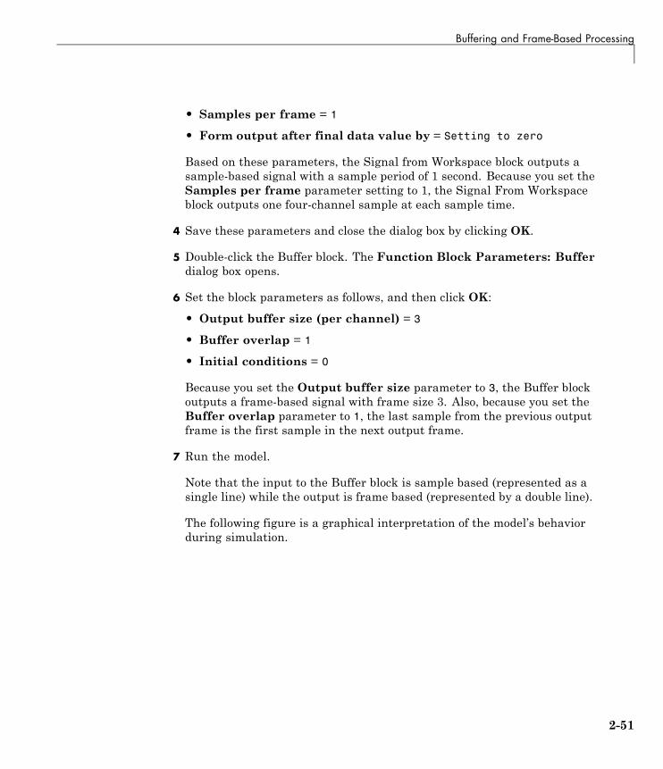
Buffering and Frame-Based Processing
• Samples per frame = 1
• Form output after final data value by = Setting to zero
Based on these parameters, the Signal from Workspace block outputs asample-based signal with a sample period of 1 second. Because you set theSamples per frame parameter setting to 1, the Signal From Workspaceblock outputs one four-channel sample at each sample time.
4 Save these parameters and close the dialog box by clicking OK.
5 Double-click the Buffer block. The Function Block Parameters: Bufferdialog box opens.
6 Set the block parameters as follows, and then click OK:
• Output buffer size (per channel) = 3
• Buffer overlap = 1
• Initial conditions = 0
Because you set the Output buffer size parameter to 3, the Buffer blockoutputs a frame-based signal with frame size 3. Also, because you set theBuffer overlap parameter to 1, the last sample from the previous outputframe is the first sample in the next output frame.
7 Run the model.
Note that the input to the Buffer block is sample based (represented as asingle line) while the output is frame based (represented by a double line).
The following figure is a graphical interpretation of the model’s behaviorduring simulation.
2-51
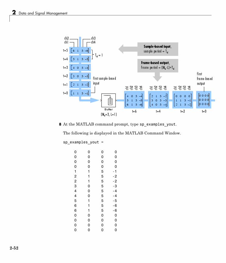
2 Data and Signal Management
8 At the MATLAB command prompt, type sp_examples_yout.
The following is displayed in the MATLAB Command Window.
sp_examples_yout =
0 0 0 00 0 0 00 0 0 00 0 0 01 1 5 -12 1 5 -22 1 5 -23 0 5 -34 0 5 -44 0 5 -45 1 5 -56 1 5 -66 1 5 -60 0 0 00 0 0 00 0 0 00 0 0 0
2-52

Buffering and Frame-Based Processing
0 0 0 0
Notice that the inputs do not begin appearing at the output until the fifthrow, the second row of the second frame. This is due to the block’s latency.
See “Excess Algorithmic Delay (Tasking Latency)” on page 2-70 for generalinformation about algorithmic delay. For instructions on how to calculatebuffering delay, see “Buffer Delay and Initial Conditions” on page 2-56.
Buffer Frame-Based Signals into Other Frame-BasedSignalsIn the following example, a two-channel frame-based signal with frame size 4is rebuffered to a frame-based signal with frame size 3 and frame period 2.Because of the overlap, the input sample period is not conserved, and theoutput sample period is 2/3:
1 At the MATLAB command prompt, type ex_buffer_tut4.
The Buffer Example T4 model opens.
2-53
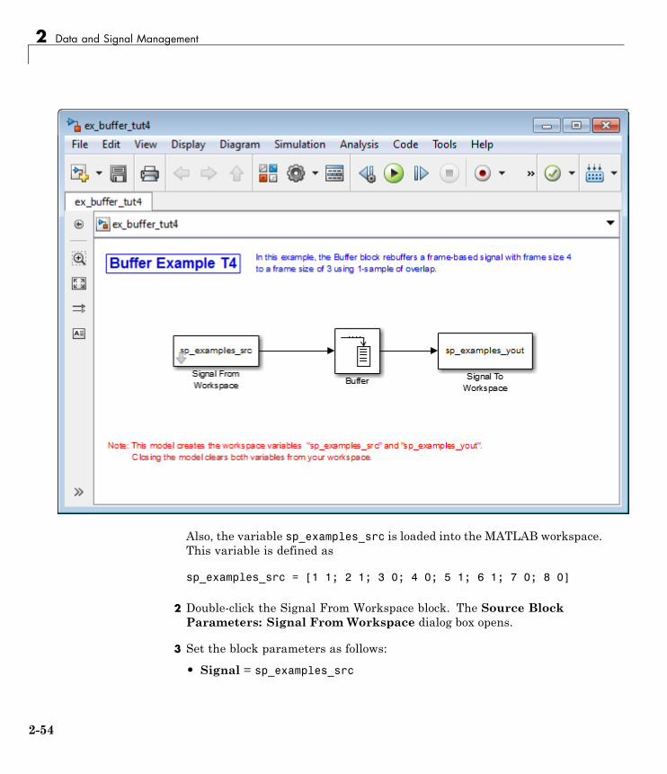
2 Data and Signal Management
Also, the variable sp_examples_src is loaded into the MATLAB workspace.This variable is defined as
sp_examples_src = [1 1; 2 1; 3 0; 4 0; 5 1; 6 1; 7 0; 8 0]
2 Double-click the Signal From Workspace block. The Source BlockParameters: Signal From Workspace dialog box opens.
3 Set the block parameters as follows:
• Signal = sp_examples_src
2-54
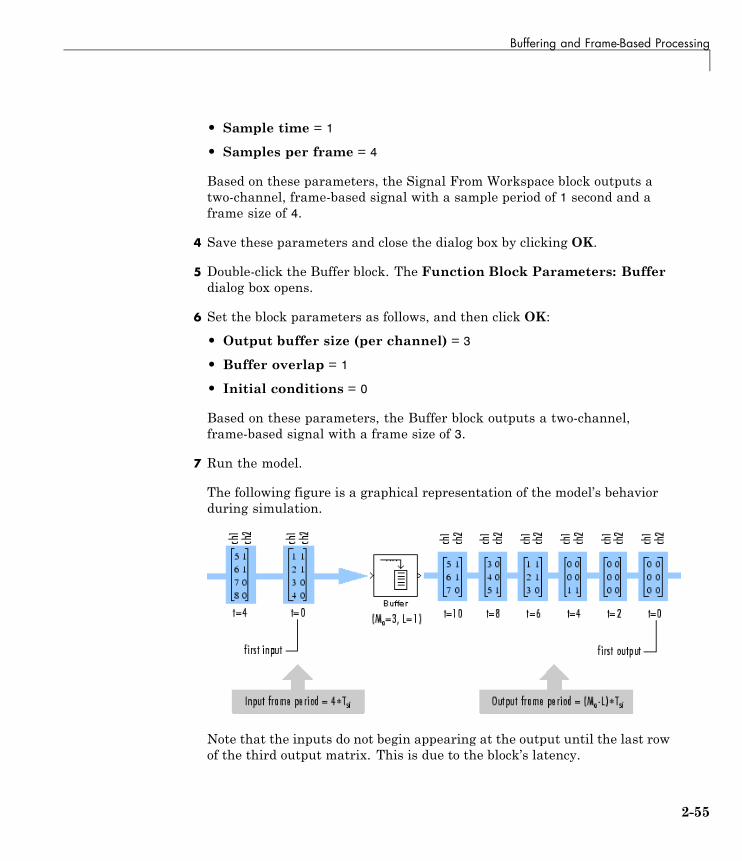
Buffering and Frame-Based Processing
• Sample time = 1
• Samples per frame = 4
Based on these parameters, the Signal From Workspace block outputs atwo-channel, frame-based signal with a sample period of 1 second and aframe size of 4.
4 Save these parameters and close the dialog box by clicking OK.
5 Double-click the Buffer block. The Function Block Parameters: Bufferdialog box opens.
6 Set the block parameters as follows, and then click OK:
• Output buffer size (per channel) = 3
• Buffer overlap = 1
• Initial conditions = 0
Based on these parameters, the Buffer block outputs a two-channel,frame-based signal with a frame size of 3.
7 Run the model.
The following figure is a graphical representation of the model’s behaviorduring simulation.
Note that the inputs do not begin appearing at the output until the last rowof the third output matrix. This is due to the block’s latency.
2-55

2 Data and Signal Management
See “Excess Algorithmic Delay (Tasking Latency)” on page 2-70 for generalinformation about algorithmic delay. For instructions on how to calculatebuffering delay, and see “Buffer Delay and Initial Conditions” on page 2-56.
Buffer Delay and Initial ConditionsIn the examples “Buffer Sample-Based Signals into Frame-Based Signalswith Overlap” on page 2-49 and “Buffer Frame-Based Signals into OtherFrame-Based Signals” on page 2-53, the input signal is delayed by a certainnumber of samples. The initial output samples correspond to the valuespecified for the Initial condition parameter. The initial condition is zeroin both examples mentioned above.
Under most conditions, the Buffer and Unbuffer blocks have some amount ofdelay or latency. This latency depends on both the block parameter settingsand the Simulink tasking mode. You can use the rebuffer_delay functionto determine the length of the block’s latency for any combination of framesize and overlap.
The syntax rebuffer_delay(f,n,v) returns the delay, in samples,introduced by the buffering and unbuffering blocks during multitaskingoperations, where f is the input frame size, n is the Output buffer sizeparameter setting, and v is the Buffer overlap parameter setting.
For example, you can calculate the delay for the model discussed in the“Buffer Frame-Based Signals into Other Frame-Based Signals” on page 2-53using the following command at the MATLAB command line:
d = rebuffer_delay(4,3,1)d = 8
This result agrees with the block’s output in that example. Notice that thismodel was simulated in Simulink multitasking mode.
For more information about delay, see “Excess Algorithmic Delay (TaskingLatency)” on page 2-70. For delay information about a specific block, see the“Latency” section of the block reference page. For more information about therebuffer_delay function, see rebuffer_delay.
2-56

Buffering and Frame-Based Processing
Unbuffer Frame-Based Signals into Sample-BasedSignalsYou can unbuffer multichannel frame-based signals into multichannelsample-based signals using the Unbuffer block. The Unbuffer block performsthe inverse operation of the Buffer block’s “sample-based to frame-based”buffering process, and generates an N-channel sample-based output from anN-channel frame-based input. The first row in each input matrix is alwaysthe first sample-based output.
The following figure is a graphical representation of this process.
The sample period of the sample-based output, Tso, is related to the inputframe period, Tfi, by the input frame size, Mi.
T T Mso fi i= /
The Unbuffer block always preserves the signal’s sample period (Tso = Tsi).See “Convert Sample and Frame Rates in Simulink” on page 2-20 for moreinformation about rate conversions.
2-57
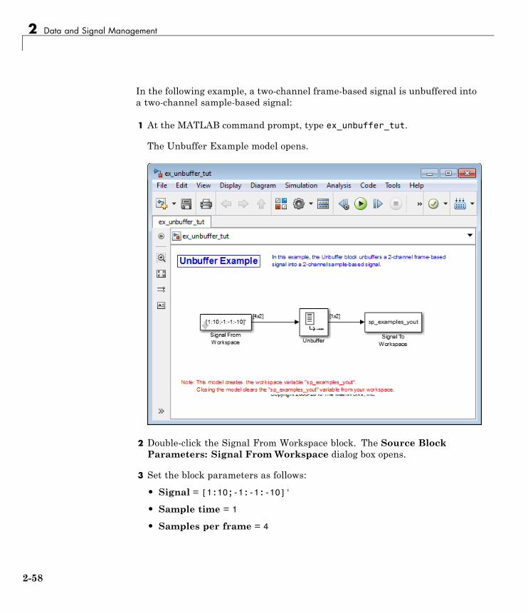
2 Data and Signal Management
In the following example, a two-channel frame-based signal is unbuffered intoa two-channel sample-based signal:
1 At the MATLAB command prompt, type ex_unbuffer_tut.
The Unbuffer Example model opens.
2 Double-click the Signal From Workspace block. The Source BlockParameters: Signal From Workspace dialog box opens.
3 Set the block parameters as follows:
• Signal = [1:10;-1:-1:-10]'
• Sample time = 1
• Samples per frame = 4
2-58

Buffering and Frame-Based Processing
• Form output after final data value by = Setting to zero
Based on these parameters, the Signal From Workspace block outputs atwo-channel, frame based-signal with frame size 4.
4 Save these parameters and close the dialog box by clicking OK.
5 Double-click the Unbuffer block. The Function Block Parameters:Unbuffer dialog box opens.
6 Set the Initial conditions parameter to 0, and then click OK.
The Unbuffer block unbuffers the frame-based signal into a two-channelsample-based signal.
7 Run the model.
The following figures is a graphical representation of what happens duringthe model simulation.
[4 -4] [3 -3] [2 -2] [1 -1]
t = 7 t = 6 t = 5 t = 4
1 -12 -23 -34 -4
2-channel frame-based signalFour consecutive samples from a2-channel sample-based signal
Note The Unbuffer block generates initial conditions not shown in thefigure below with the value specified by the Initial conditions parameter.See the Unbuffer reference page for information about the number of initialconditions that appear in the output.
8 At the MATLAB command prompt, type sp_examples_yout.
The following is a portion of the output.
2-59
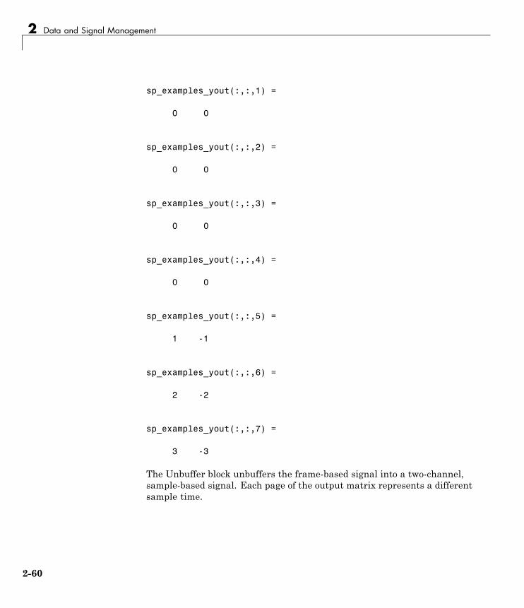
2 Data and Signal Management
sp_examples_yout(:,:,1) =
0 0
sp_examples_yout(:,:,2) =
0 0
sp_examples_yout(:,:,3) =
0 0
sp_examples_yout(:,:,4) =
0 0
sp_examples_yout(:,:,5) =
1 -1
sp_examples_yout(:,:,6) =
2 -2
sp_examples_yout(:,:,7) =
3 -3
The Unbuffer block unbuffers the frame-based signal into a two-channel,sample-based signal. Each page of the output matrix represents a differentsample time.
2-60
Delay and Latency
Delay and Latency
Note Starting in R2010b, many DSP System Toolbox blocks received a newparameter to control whether they perform sample- or frame-based processing.The following content has not been updated to reflect this change. For moreinformation, see the “Frame-Based Processing” section of the Release Notes.
In this section...
“Computational Delay” on page 2-61
“Algorithmic Delay” on page 2-63
“Zero Algorithmic Delay” on page 2-63
“Basic Algorithmic Delay” on page 2-66
“Excess Algorithmic Delay (Tasking Latency)” on page 2-70
“Predict Tasking Latency” on page 2-72
Computational DelayThe computational delay of a block or subsystem is related to the numberof operations involved in executing that block or subsystem. For example,an FFT block operating on a 256-sample input requires Simulink softwareto perform a certain number of multiplications for each input frame. Theactual amount of time that these operations consume depends heavily on theperformance of both the computer hardware and underlying software layers,such as the MATLAB environment and the operating system. Therefore,computational delay for a particular model can vary from one computerplatform to another.
The simulation time represented on a model’s status bar, which canbe accessed via the Simulink Digital Clock block, does not provide anyinformation about computational delay. For example, according to theSimulink timer, the FFT mentioned above executes instantaneously, withno delay whatsoever. An input to the FFT block at simulation time t=25.0is processed and output at simulation time t=25.0, regardless of the number
2-61

2 Data and Signal Management
of operations performed by the FFT algorithm. The Simulink timer reflectsonly algorithmic delay, not computational delay.
Reduce Computational DelayThere are a number of ways to reduce computational delay without actuallyrunning the simulation on faster hardware. To begin with, you shouldfamiliarize yourself with “Model Execution Profiling” in the Simulinkdocumentation, which describes some basic strategies. The followinginformation discusses several options for improving performance.
A first step in improving performance is to analyze your model, and eliminateor simplify elements that are adding excessively to the computational load.Such elements might include scope displays and data logging blocks that youhad put in place for debugging purposes and no longer require. In addition tothese model-specific adjustments, there are a number of more general stepsyou can take to improve the performance of any model:
• Use frame-based processing wherever possible. It is advantageous for theentire model to be frame based. See “Benefits of Frame-Based Processing”on page 2-6 for more information.
• Use the dspstartup file to tailor Simulink for signal processing models, ormanually make the adjustments described in “Settings in dspstartup.m” inthe DSP System Toolbox Getting Started Guide.
• Turn off the Simulink status bar by deselecting the Status bar option inthe View menu. Simulation speed will improve, but the time indicatorwill not be visible.
• Run your simulation from the MATLAB command line by typing
sim(gcs)
This method of starting a simulation can greatly increase the simulationspeed, but also has several limitations:
- You cannot interact with the simulation (to tune parameters, forinstance).
- You must press Ctrl+C to stop the simulation, or specify start andstop times.
2-62

Delay and Latency
- There are no graphics updates in M-file S-functions, which includeblocks such as Vector Scope, etc.
• Use Simulink Coder code generation software to generate generic real-time(GRT) code targeted to your host platform, and run the model using thegenerated executable file. See the Simulink Coder documentation for moreinformation.
Algorithmic DelayAlgorithmic delay is delay that is intrinsic to the algorithm of a block orsubsystem and is independent of CPU speed. In this guide, the algorithmicdelay of a block is referred to simply as the block’s delay. It is generallyexpressed in terms of the number of samples by which a block’s output lagsbehind the corresponding input. This delay is directly related to the timeelapsed on the Simulink timer during that block’s execution.
The algorithmic delay of a particular block may depend on both the blockparameter settings and the general Simulink settings. To simplify matters, itis helpful to categorize a block’s delay using the following categories:
• “Zero Algorithmic Delay” on page 2-63
• “Basic Algorithmic Delay” on page 2-66
• “Excess Algorithmic Delay (Tasking Latency)” on page 2-70
The following topics explain the different categories of delay, and howthe simulation and parameter settings can affect the level of delay that aparticular block experiences.
Zero Algorithmic DelayThe FFT block is an example of a component that has no algorithmic delay.The Simulink timer does not record any passage of time while the blockcomputes the FFT of the input, and the transformed data is available at theoutput in the same time step that the input is received. There are many otherblocks that have zero algorithmic delay, such as the blocks in the Matricesand Linear Algebra libraries. Each of those blocks processes its input andgenerates its output in a single time step.
The Normalization block is an example of a block with zero algorithmic delay:
2-63
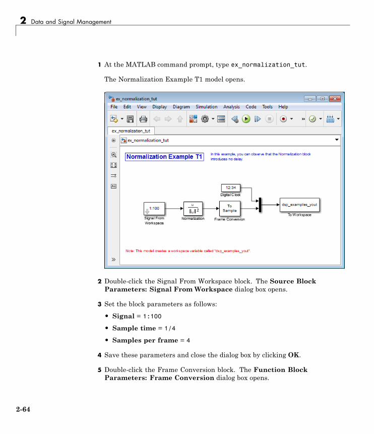
2 Data and Signal Management
1 At the MATLAB command prompt, type ex_normalization_tut.
The Normalization Example T1 model opens.
2 Double-click the Signal From Workspace block. The Source BlockParameters: Signal From Workspace dialog box opens.
3 Set the block parameters as follows:
• Signal = 1:100
• Sample time = 1/4
• Samples per frame = 4
4 Save these parameters and close the dialog box by clicking OK.
5 Double-click the Frame Conversion block. The Function BlockParameters: Frame Conversion dialog box opens.
2-64

Delay and Latency
6 Set the Sampling mode of output signal parameter to Sample based,and then click OK.
7 Run the model.
The model prepends the current value of the Simulink timer output fromthe Digital Clock block to each output frame. The Frame Conversion blockconverts the frame-based signal to a sample-based signal so that the outputin the MATLAB Command Window is more easily readable.
The Signal From Workspace block generates a new frame containing foursamples once every second (Tfo = π*4). The first few output frames are:
(t=0) [ 1 2 3 4]'(t=1) [ 5 6 7 8]'(t=2) [ 9 10 11 12]'(t=3) [13 14 15 16]'(t=4) [17 18 19 20]'
8 At the MATLAB command prompt, type squeeze(dsp_examples_yout)'.
The normalized output, dsp_examples_yout, is converted to aneasier-to-read matrix format. The result, ans, is shown in the followingfigure:
ans =
0 0.0333 0.0667 0.1000 0.13331.0000 0.0287 0.0345 0.0402 0.04602.0000 0.0202 0.0224 0.0247 0.02693.0000 0.0154 0.0165 0.0177 0.01894.0000 0.0124 0.0131 0.0138 0.01465.0000 0.0103 0.0108 0.0113 0.0118
The first column of ans is the Simulink time provided by the Digital Clockblock. You can see that the squared 2-norm of the first input,
[1 2 3 4]' ./ sum([1 2 3 4]'.^2)
2-65

2 Data and Signal Management
appears in the first row of the output (at time t=0), the same time step thatthe input was received by the block. This indicates that the Normalizationblock has zero algorithmic delay.
Zero Algorithmic Delay and Algebraic LoopsWhen several blocks with zero algorithmic delay are connected in a feedbackloop, Simulink may report an algebraic loop error and performance maygenerally suffer. You can prevent algebraic loops by injecting at least onesample of delay into a feedback loop , for example, by including a Delay blockwith Delay > 0. For more information, see “Algebraic Loops” in the Simulinkdocumentation.
Basic Algorithmic DelayThe Variable Integer Delay block is an example of a block with algorithmicdelay. In the following example, you use this block to demonstrate thisconcept:
1 At the MATLAB command prompt, type ex_variableintegerdelay_tut.
The Variable Integer Delay Example T1 opens.
2-66

Delay and Latency
2 Double-click the Signal From Workspace block. The Source BlockParameters: Signal From Workspace dialog box opens.
3 Set the block parameters as follows:
• Signal = 1:100
• Sample time = 1
• Samples per frame = 1
4 Save these parameters and close the dialog box by clicking OK.
5 Double-click the Constant block. The Source Block Parameters:Constant dialog box opens.
6 Set the block parameters as follows:
• Constant value = 3
• Interpret vector parameters as 1–D = Clear this check box
2-67

2 Data and Signal Management
• Sampling mode = Sample based
• Sample time = 1
Click OK to save these parameters and close the dialog box.
The input to the Delay port of the Variable Integer Delay block specifiesthe number of sample periods that should elapse before an input to the Inport is released to the output. This value represents the block’s algorithmicdelay. In this example, since the input to the Delay port is 3, and thesample period at the In and Delay ports is 1, then the sample that arrivesat the block’s In port at time t=0 is released to the output at time t=3.
7 Double-click the Variable Integer Delay block. The Function BlockParameters: Variable Integer Delay dialog box opens.
8 Set the Initial conditions parameter to -1, and then click OK.
9 From the Display menu, point to Signals & Ports, and select SignalDimensions and Wide Nonscalar Lines.
10 Run the model.
The model should look similar to the following figure.
2-68
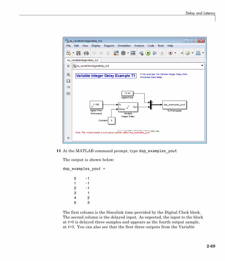
Delay and Latency
11 At the MATLAB command prompt, type dsp_examples_yout
The output is shown below:
dsp_examples_yout =
0 -11 -12 -13 14 25 3
The first column is the Simulink time provided by the Digital Clock block.The second column is the delayed input. As expected, the input to the blockat t=0 is delayed three samples and appears as the fourth output sample,at t=3. You can also see that the first three outputs from the Variable
2-69

2 Data and Signal Management
Integer Delay block inherit the value of the block’s Initial conditionsparameter, -1. This period of time, from the start of the simulation untilthe first input is propagated to the output, is sometimes called the initialdelay of the block.
Many DSP System Toolbox blocks have some degree of fixed or adjustablealgorithmic delay. These include any blocks whose algorithms rely on delayor storage elements, such as filters or buffers. Often, but not always, suchblocks provide an Initial conditions parameter that allows you to specifythe output values generated by the block during the initial delay. In othercases, the initial conditions are internally set to 0.
Consult the block reference pages for the delay characteristics of specificDSP System Toolbox blocks.
Excess Algorithmic Delay (Tasking Latency)Under certain conditions, Simulink may force a block to delay inputs longerthan is strictly required by the block’s algorithm. This excess algorithmicdelay is called tasking latency, because it arises from synchronizationrequirements of the Simulink tasking mode. A block’s overall algorithmicdelay is the sum of its basic delay and tasking latency.
Algorithmic delay = Basic algorithmic delay + Tasking latency
The tasking latency for a particular block may be dependent on the followingblock and model characteristics:
• “Simulink Tasking Mode” on page 2-70
• “Block Rate Type” on page 2-71
• “Model Rate Type” on page 2-71
• “Block Sample Mode” on page 2-72
Simulink Tasking ModeSimulink has two tasking modes:
• Single-tasking
2-70
Delay and Latency
• Multitasking
To select a mode, from the Simulation menu, selectModel ConfigurationParameters. In the Select pane, click Solver. From the Type list, selectFixed-step. From the Tasking mode for periodic sample times list,choose SingleTasking or MultiTasking. If, from the Tasking modefor periodic sample times list you select Auto, the simulation runs insingle-tasking mode if the model is single-rate, or multitasking mode if themodel is multirate.
Note Many multirate blocks have reduced latency in the Simulinksingle-tasking mode. Check the “Latency” section of a multirate block’sreference page for details. Also see “Scheduling” in the Simulink Coder User’sGuide.
Block Rate TypeA block is called single-rate when all of its input and output ports operate atthe same frame rate. A block is called multirate when at least one input oroutput port has a different frame rate than the others.
Many blocks are permanently single-rate. This means that all input andoutput ports always have the same frame rate. For other blocks, the blockparameter settings determine whether the block is single-rate or multirate.Only multirate blocks are subject to tasking latency.
Note Simulink may report an algebraic loop error if it detects a feedbackloop composed entirely of multirate blocks. To break such an algebraic loop,insert a single-rate block with nonzero delay, such as a Unit Delay block. Seethe Simulink documentation for more information about “Algebraic Loops”.
Model Rate TypeWhen all ports of all blocks in a model operate at a single frame rate, themodel is called single-rate. When the model contains blocks with differingframe rates, or at least one multirate block, the model is called multirate.
2-71

2 Data and Signal Management
Note that Simulink prevents a single-rate model from running in multitaskingmode by generating an error.
Block Sample ModeMany blocks can operate in either sample-based or frame-based modes. Insource blocks, the mode is usually determined by the Samples per frameparameter. If, for the Samples per frame parameter, you enter 1, the blockoperates in sample-based mode. If you enter a value greater than 1, the blockoperates in frame-based mode. In nonsource blocks, the sample mode isdetermined by the input signal. See the block reference pages for additionalinformation about specific blocks.
Predict Tasking LatencyThe specific amount of tasking latency created by a particular combinationof block parameter and simulation settings is discussed in the “Latency”section of a block’s reference page. In this topic, you use the Upsample block’sreference page to predict the tasking latency of a model:
1 At the MATLAB command prompt, type ex_upsample_tut1.
The Upsample Example T1 model opens.
2-72
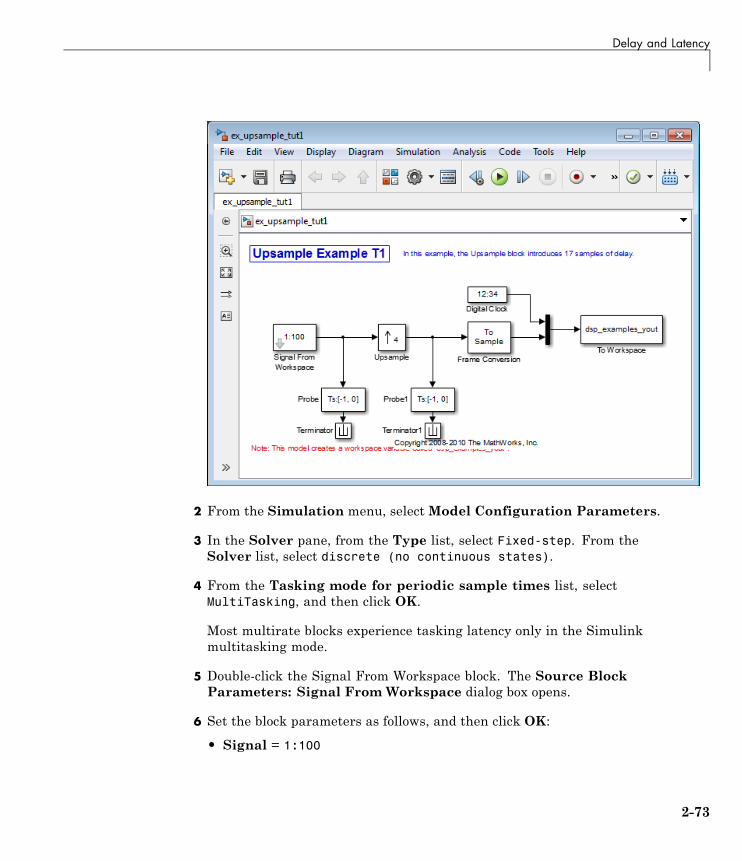
Delay and Latency
2 From the Simulation menu, selectModel Configuration Parameters.
3 In the Solver pane, from the Type list, select Fixed-step. From theSolver list, select discrete (no continuous states).
4 From the Tasking mode for periodic sample times list, selectMultiTasking, and then click OK.
Most multirate blocks experience tasking latency only in the Simulinkmultitasking mode.
5 Double-click the Signal From Workspace block. The Source BlockParameters: Signal From Workspace dialog box opens.
6 Set the block parameters as follows, and then click OK:
• Signal = 1:100
2-73

2 Data and Signal Management
• Sample time = 1/4
• Samples per frame = 4
• Form output after final data value by = Setting to zero
7 Double-click the Upsample block. The Function Block Parameters:Upsample dialog box opens.
8 Set the block parameters as follows, and then click OK:
• Upsample factor, L = 4
• Sample offset (0 to L-1) = 0
• Input processing = Columns as channels (frame based)
• Rate options = Allow multirate processing
• Initial condition = -1
The Rate options parameter makes the model multirate, since the inputand output frame rates will not be equal.
9 Double-click the Digital Clock block. The Source Block Parameters:Digital Clock dialog box opens.
10 Set the Sample time parameter to 0.25, and then click OK.
This matches the sample period of the Upsample block’s output.
11 Double-click the Frame Conversion block. The Function BlockParameters: Frame Conversion dialog box opens.
12 Set the Sampling mode of output signal parameter to Sample based,and then click OK.
13 Run the model.
The model should now look similar to the following figure.
2-74
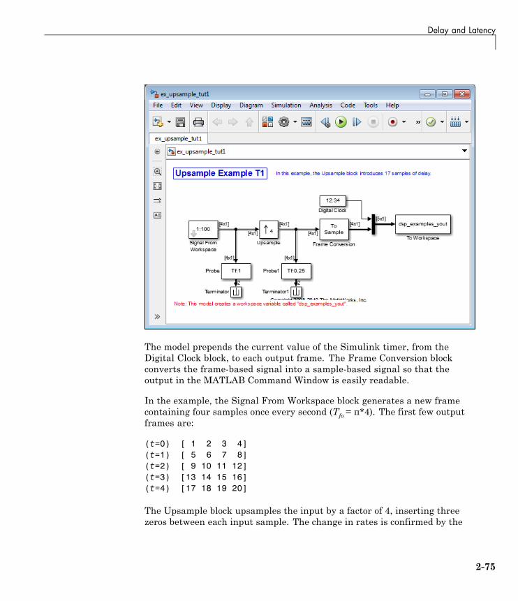
Delay and Latency
The model prepends the current value of the Simulink timer, from theDigital Clock block, to each output frame. The Frame Conversion blockconverts the frame-based signal into a sample-based signal so that theoutput in the MATLAB Command Window is easily readable.
In the example, the Signal From Workspace block generates a new framecontaining four samples once every second (Tfo = π*4). The first few outputframes are:
(t=0) [ 1 2 3 4](t=1) [ 5 6 7 8](t=2) [ 9 10 11 12](t=3) [13 14 15 16](t=4) [17 18 19 20]
The Upsample block upsamples the input by a factor of 4, inserting threezeros between each input sample. The change in rates is confirmed by the
2-75
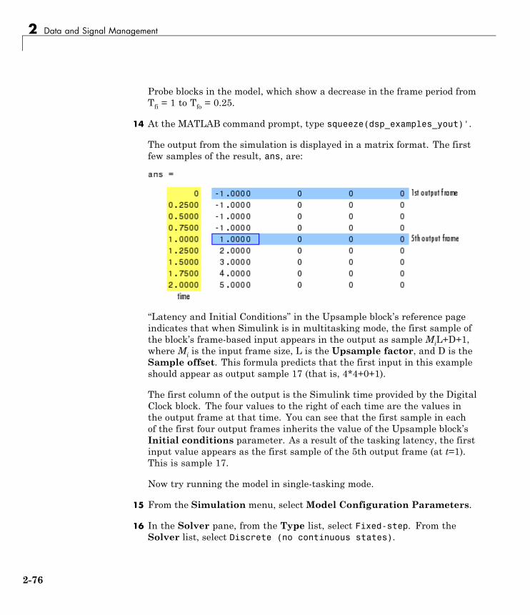
2 Data and Signal Management
Probe blocks in the model, which show a decrease in the frame period fromTfi = 1 to Tfo = 0.25.
14 At the MATLAB command prompt, type squeeze(dsp_examples_yout)'.
The output from the simulation is displayed in a matrix format. The firstfew samples of the result, ans, are:
“Latency and Initial Conditions” in the Upsample block’s reference pageindicates that when Simulink is in multitasking mode, the first sample ofthe block’s frame-based input appears in the output as sample MiL+D+1,where Mi is the input frame size, L is the Upsample factor, and D is theSample offset. This formula predicts that the first input in this exampleshould appear as output sample 17 (that is, 4*4+0+1).
The first column of the output is the Simulink time provided by the DigitalClock block. The four values to the right of each time are the values inthe output frame at that time. You can see that the first sample in eachof the first four output frames inherits the value of the Upsample block’sInitial conditions parameter. As a result of the tasking latency, the firstinput value appears as the first sample of the 5th output frame (at t=1).This is sample 17.
Now try running the model in single-tasking mode.
15 From the Simulation menu, selectModel Configuration Parameters.
16 In the Solver pane, from the Type list, select Fixed-step. From theSolver list, select Discrete (no continuous states).
2-76
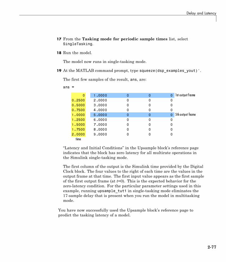
Delay and Latency
17 From the Tasking mode for periodic sample times list, selectSingleTasking.
18 Run the model.
The model now runs in single-tasking mode.
19 At the MATLAB command prompt, type squeeze(dsp_examples_yout)'.
The first few samples of the result, ans, are:
“Latency and Initial Conditions” in the Upsample block’s reference pageindicates that the block has zero latency for all multirate operations inthe Simulink single-tasking mode.
The first column of the output is the Simulink time provided by the DigitalClock block. The four values to the right of each time are the values in theoutput frame at that time. The first input value appears as the first sampleof the first output frame (at t=0). This is the expected behavior for thezero-latency condition. For the particular parameter settings used in thisexample, running upsample_tut1 in single-tasking mode eliminates the17-sample delay that is present when you run the model in multitaskingmode.
You have now successfully used the Upsample block’s reference page topredict the tasking latency of a model.
2-77

2 Data and Signal Management
2-78

3
Filter Analysis, Design, andImplementation
• “Design a Filter in Fdesign — Process Overview” on page 3-2
• “Design a Filter in the Filterbuilder GUI” on page 3-11
• “Use FDATool with DSP System Toolbox Software” on page 3-16
• “Digital Frequency Transformations” on page 3-88
• “Digital Filter Design Block” on page 3-123
• “Filter Realization Wizard” on page 3-134
• “Digital Filter Block” on page 3-147
• “Analog Filter Design Block” on page 3-159
3 Filter Analysis, Design, and Implementation
Design a Filter in Fdesign — Process Overview
Process Flow Diagram and Filter Design Methodology
• “Exploring the Process Flow Diagram” on page 3-2
• “Select a Response” on page 3-4
• “Select a Specification” on page 3-4
• “Select an Algorithm” on page 3-6
• “Customize the Algorithm” on page 3-8
• “Design the Filter” on page 3-8
• “Design Analysis” on page 3-9
• “Realize or Apply the Filter to Input Data” on page 3-10
Note You must minimally have the Signal Processing Toolbox™ installedto use fdesign and design. Some of the features described below maybe unavailable if your installation does not additionally include the DSPSystem Toolbox license. The DSP System Toolbox significantly expands thefunctionality available for the specification, design, and analysis of filters.You can verify the presence of both toolboxes by typing ver at the commandprompt.
Exploring the Process Flow DiagramThe process flow diagram shown in the following figure lists the steps andshows the order of the filter design process.
3-2
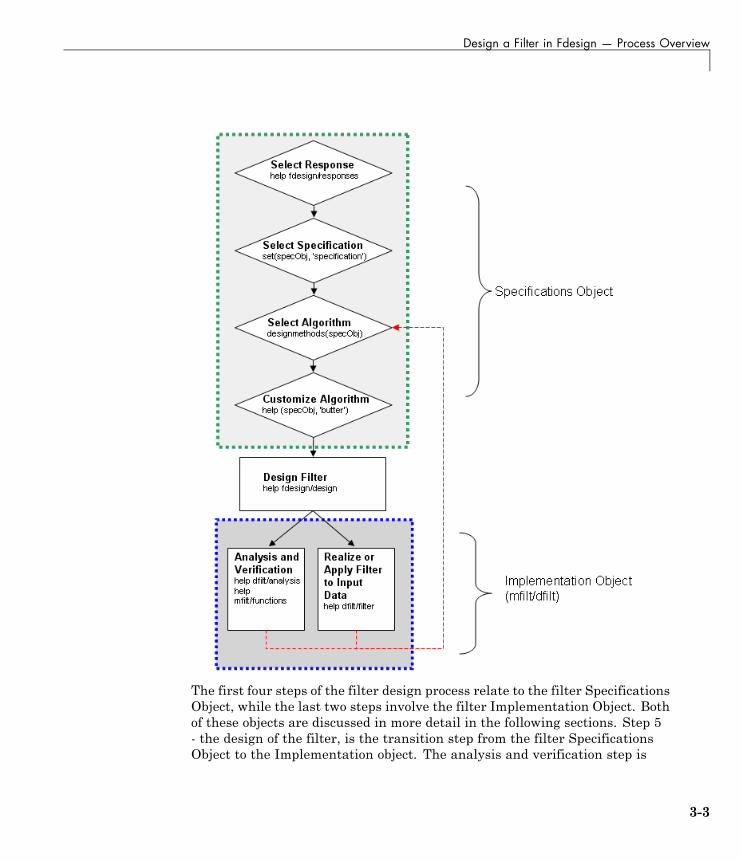
Design a Filter in Fdesign — Process Overview
The first four steps of the filter design process relate to the filter SpecificationsObject, while the last two steps involve the filter Implementation Object. Bothof these objects are discussed in more detail in the following sections. Step 5- the design of the filter, is the transition step from the filter SpecificationsObject to the Implementation object. The analysis and verification step is
3-3

3 Filter Analysis, Design, and Implementation
completely optional. It provides methods for the filter designer to ensure thatthe filter complies with all design criteria. Depending on the results of thisverification, you can loop back to steps 3 and 4, to either choose a differentalgorithm, or to customize the current one. You may also wish to go back tosteps 3 or 4 after you filter the input data with the designed filter (step 7),and find that you wish to tweak the filter or change it further.
The diagram shows the help command for each step. Enter the help line at theMATLAB command prompt to receive instructions and further documentationlinks for the particular step. Not all of the steps have to be executed explicitly.For example, you could go from step 1 directly to step 5, and the interim threesteps are done for you by the software.
The following are the details for each of the steps shown above.
Select a ResponseIf you type:
help fdesign/responses
at the MATLAB command prompt, you see a list of all available filterresponses. The responses marked with an asterisk require the DSP SystemToolbox.
You must select a response to initiate the filter. In this example, a bandpassfilter Specifications Object is created by typing the following:
d = fdesign.bandpass
Select a SpecificationA specification is an array of design parameters for a given filter. Thespecification is a property of the Specifications Object.
Note A specification is not the same as the Specifications Object. ASpecifications Object contains a specification as one of its properties.
3-4
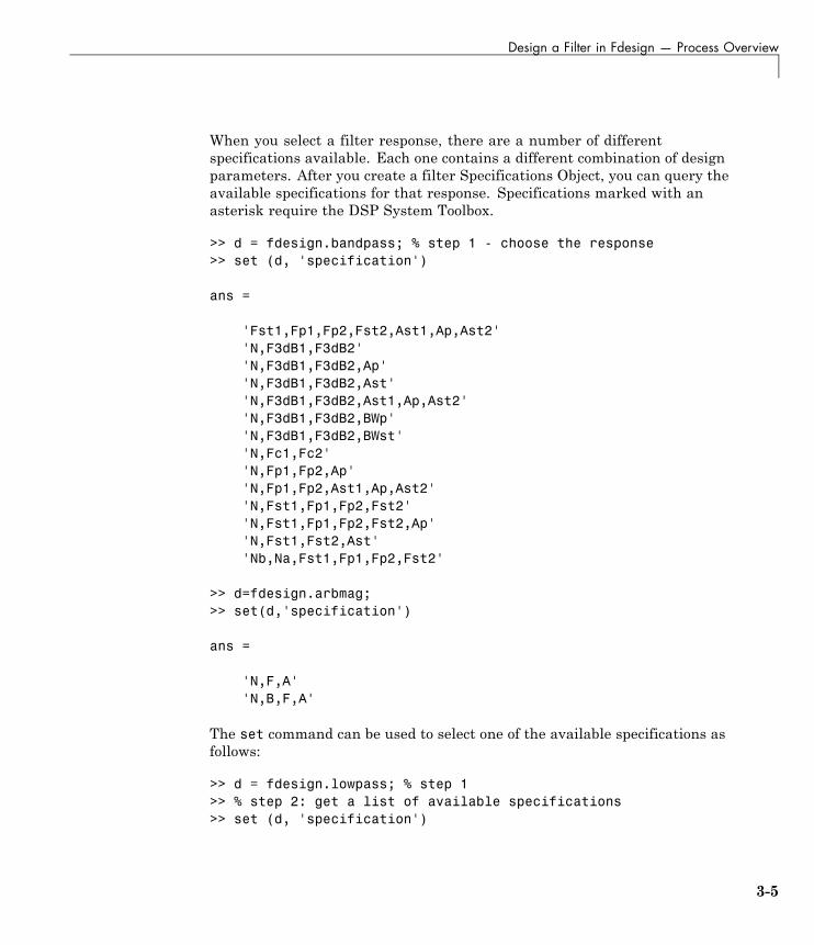
Design a Filter in Fdesign — Process Overview
When you select a filter response, there are a number of differentspecifications available. Each one contains a different combination of designparameters. After you create a filter Specifications Object, you can query theavailable specifications for that response. Specifications marked with anasterisk require the DSP System Toolbox.
>> d = fdesign.bandpass; % step 1 - choose the response>> set (d, 'specification')
ans =
'Fst1,Fp1,Fp2,Fst2,Ast1,Ap,Ast2''N,F3dB1,F3dB2''N,F3dB1,F3dB2,Ap''N,F3dB1,F3dB2,Ast''N,F3dB1,F3dB2,Ast1,Ap,Ast2''N,F3dB1,F3dB2,BWp''N,F3dB1,F3dB2,BWst''N,Fc1,Fc2''N,Fp1,Fp2,Ap''N,Fp1,Fp2,Ast1,Ap,Ast2''N,Fst1,Fp1,Fp2,Fst2''N,Fst1,Fp1,Fp2,Fst2,Ap''N,Fst1,Fst2,Ast''Nb,Na,Fst1,Fp1,Fp2,Fst2'
>> d=fdesign.arbmag;>> set(d,'specification')
ans =
'N,F,A''N,B,F,A'
The set command can be used to select one of the available specifications asfollows:
>> d = fdesign.lowpass; % step 1>> % step 2: get a list of available specifications>> set (d, 'specification')
3-5

3 Filter Analysis, Design, and Implementation
ans =
'Fp,Fst,Ap,Ast''N,F3dB''N,F3dB,Ap''N,F3dB,Ap,Ast''N,F3dB,Ast''N,F3dB,Fst''N,Fc''N,Fc,Ap,Ast''N,Fp,Ap''N,Fp,Ap,Ast''N,Fp,F3dB''N,Fp,Fst''N,Fp,Fst,Ap''N,Fp,Fst,Ast''N,Fst,Ap,Ast''N,Fst,Ast''Nb,Na,Fp,Fst'
>> %step 2: set the required specification>> set (d, 'specification', 'N,Fc')
If you do not perform this step explicitly, fdesign returns the defaultspecification for the response you chose in “Select a Response” on page 3-4, andprovides default values for all design parameters included in the specification.
Select an AlgorithmThe availability of algorithms depends the chosen filter response, the designparameters, and the availability of the DSP System Toolbox. In other words,for the same lowpass filter, changing the specification string also changes theavailable algorithms. In the following example, for a lowpass filter and aspecification of 'N, Fc', only one algorithm is available—window.
>> %step 2: set the required specification>> set (d, 'specification', 'N,Fc')>> designmethods (d) %step3: get available algorithms
Design Methods for class fdesign.lowpass (N,Fc):
3-6
Design a Filter in Fdesign — Process Overview
window
However, for a specification of 'Fp,Fst,Ap,Ast', a number of algorithms areavailable. If the user has only the Signal Processing Toolbox installed, thefollowing algorithms are available:
>>set (d, 'specification', 'Fp,Fst,Ap,Ast')>>designmethods(d)
Design Methods for class fdesign.lowpass (Fp,Fst,Ap,Ast):
buttercheby1cheby2ellipequiripplekaiserwin
If the user additionally has the DSP System Toolbox installed, the number ofavailable algorithms for this response and specification string increases:
>>set(d,'specification','Fp,Fst,Ap,Ast')>>designmethods(d)
Design Methods for class fdesign.lowpass (Fp,Fst,Ap,Ast):
buttercheby1cheby2ellipequirippleifirkaiserwinmultistage
3-7

3 Filter Analysis, Design, and Implementation
The user chooses a particular algorithm and implements the filter with thedesign function.
>>Hd=design(d,'butter');
The preceding code actually creates the filter, where Hd is the filterImplementation Object. This concept is discussed further in the next step.
If you do not perform this step explicitly, design automatically selects theoptimum algorithm for the chosen response and specification.
Customize the AlgorithmThe customization options available for any given algorithm depend not onlyon the algorithm itself, selected in “Select an Algorithm” on page 3-6, but alsoon the specification selected in “Select a Specification” on page 3-4. To exploreall the available options, type the following at the MATLAB command prompt:
help (d, 'algorithm-name')
where d is the Filter Specification Object, and algorithm-name is the name ofthe algorithm in single quotes, such as 'butter' or 'cheby1'.
The application of these customization options takes place while “Designthe Filter” on page 3-8, because these options are the properties of the filterImplementation Object, not the Specification Object.
If you do not perform this step explicitly, the optimum algorithm structure isselected.
Design the FilterThis next task introduces a new object, the Filter Object, or dfilt. To createa filter, use the design command:
>> % design filter w/o specifying the algorithm>> Hd = design(d);
where Hd is the Filter Object and d is the Specifications Object. This codecreates a filter without specifying the algorithm. When the algorithm is notspecified, the software selects the best available one.
3-8

Design a Filter in Fdesign — Process Overview
To apply the algorithm chosen in “Select an Algorithm” on page 3-6, use thesame design command, but specify the Butterworth algorithm as follows:
>> Hd = design(d, 'butter');
where Hd is the new Filter Object, and d is the Specifications Object.
To obtain help and see all the available options, type:
>> help fdesign/design
This help command describes not only the options for the design commanditself, but also options that pertain to the method or the algorithm. If youare customizing the algorithm, you apply these options in this step. In thefollowing example, you design a bandpass filter, and then modify the filterstructure:
>> Hd = design(d, 'butter', 'filterstructure', 'df2sos')
f =
FilterStructure: 'Direct-Form II, Second-Order Sections'Arithmetic: 'double'sosMatrix: [7x6 double]
ScaleValues: [8x1 double]PersistentMemory: false
The filter design step, just like the first task of choosing a response, must beperformed explicitly. A Filter Object is created only when design is called.
Design AnalysisAfter the filter is designed you may wish to analyze it to determine if the filtersatisfies the design criteria. Filter analysis is broken into three main sections:
• Frequency domain analysis — Includes the magnitude response, groupdelay, and pole-zero plots.
• Time domain analysis — Includes impulse and step response
• Implementation analysis — Includes quantization noise and cost
3-9
3 Filter Analysis, Design, and Implementation
To display help for analysis of a discrete-time filter, type:
>> help dfilt/analysis
To display help for analysis of a multirate filter, type:
>> help mfilt/functions
To analyze your filter, you must explicitly perform this step.
Realize or Apply the Filter to Input DataAfter the filter is designed and optimized, it can be used to filter actual inputdata. The basic filter command takes input data x, filters it through the FilterObject, and produces output y:
>> y = filter (FilterObj, x)
This step is never automatically performed for you. To filter your data, youmust explicitly execute this step. To understand how the filtering commandswork, type:
>> help dfilt/filter
Note If you have Simulink, you have the option of exporting this filterto a Simulink block using the realizemdl command. To get help on thiscommand, type:
>> help realizemdl
3-10

Design a Filter in the Filterbuilder GUI
Design a Filter in the Filterbuilder GUI
The Graphical Interface to Fdesign
• “Introduction to Filterbuilder” on page 3-11
• “Filterbuilder Design Process” on page 3-11
• “Select a Response” on page 3-12
• “Select a Specification” on page 3-13
• “Select an Algorithm” on page 3-13
• “Customize the Algorithm” on page 3-13
• “Analyze the Design” on page 3-13
• “Realize or Apply the Filter to Input Data” on page 3-14
Introduction to FilterbuilderThe filterbuilder function provides a graphical interface to thefdesign object-oriented filter design paradigm and is intended to reducedevelopment time during the filter design process. filterbuilder uses aspecification-centered approach to find the best filter for the desired response.
Note filterbuilder requires the Signal Processing Toolbox. Thefunctionality of filterbuilder is greatly expanded by the DSP SystemToolbox. Some of the features described or displayed below are only availableif the DSP System Toolbox is installed. You may verify your installation bytyping ver at the command prompt.
Filterbuilder Design ProcessThe design process when using filterbuilder is similar to the processoutlined in the section titled “Process Flow Diagram and Filter DesignMethodology” in the Getting Started guide. The idea is to choose theconstraints and specifications of the filter, and to use those as a starting pointin the design. Postponing the choice of algorithm for the filter allows thebest design method to be determined automatically, based upon the desired
3-11

3 Filter Analysis, Design, and Implementation
performance criteria. The following are the details of each of the steps fordesigning a filter with filterbuilder.
Select a ResponseWhen you open the filterbuilder tool by typing:
filterbuilder
at the MATLAB command prompt, the Response Selection dialog boxappears, listing all possible filter responses available in the software. If youhave the DSP System Toolbox software installed, you have access to the fullcomplement of filter responses.
Note This step cannot be skipped because it is not automatically completedfor you by the software. You must select a response to initiate the filter designprocess.
After you choose a response, say bandpass, you start the design of theSpecifications Object, and the Bandpass Design dialog box appears.This dialog box contains a Main pane, a Data Types pane and a CodeGeneration pane. The specifications of your filter are generally set in theMain pane of the dialog box.
The Data Types pane provides settings for precision and data types, and theCode Generation pane contains options for various implementations ofthe completed filter design.
For the initial design of your filter, you will mostly use theMain pane.
The Bandpass Design dialog box contains all the parameters you need todetermine the specifications of a bandpass filter. The parameters listed inthe Main pane depend upon the type of filter you are designing. However,no matter what type of filter you have chosen in the Response Selectiondialog box, the filter design dialog box contains the Main, Data Types, andCode Generation panes.
3-12
Design a Filter in the Filterbuilder GUI
Select a SpecificationTo choose the specification for the bandpass filter, you can begin by selectingan Impulse Response, Order Mode, and Filter Type in the FilterSpecifications frame of the Main Pane. You can further specify theresponse of your filter by setting frequency and magnitude specifications inthe appropriate frames on the Main Pane.
Note Frequency, Magnitude, and Algorithm specifications areinterdependent and may change based upon your Filter Specificationsselections. When choosing specifications for your filter, select your FilterSpecifications first and work your way down the dialog box- this approachensures that the best settings for dependent specifications display as availablein the dialog box.
Select an AlgorithmThe algorithms available for your filter depend upon the filter response anddesign parameters you have selected in the previous steps. For example, in thecase of a bandpass filter, if the impulse response selected is IIR and the OrderMode field is set toMinimum, the design methods available are Butterworth,Chebyshev type I or II, or Elliptic, whereas if the Order Mode field is setto Specify, the design method available is IIR least p-norm.
Customize the AlgorithmBy expanding the Design options section of the Algorithm frame, you canfurther customize the algorithm specified. The options available will dependupon the algorithm and settings that have already been selected in the dialogbox. In the case of a bandpass IIR filter using the Butterworth method,design options such as Match Exactly are available.
Analyze the DesignTo analyze the filter response, click on the View Filter Response button. TheFilter Visualization Tool opens displaying the magnitude plot of the filterresponse.
3-13
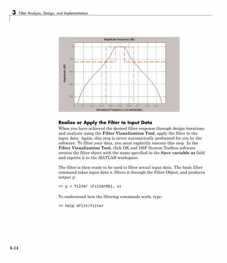
3 Filter Analysis, Design, and Implementation
Realize or Apply the Filter to Input DataWhen you have achieved the desired filter response through design iterationsand analysis using the Filter Visualization Tool, apply the filter to theinput data. Again, this step is never automatically performed for you by thesoftware. To filter your data, you must explicitly execute this step. In theFilter Visualization Tool, click OK and DSP System Toolbox softwarecreates the filter object with the name specified in the Save variable as fieldand exports it to the MATLAB workspace.
The filter is then ready to be used to filter actual input data. The basic filtercommand takes input data x, filters it through the Filter Object, and producesoutput y:
>> y = filter (FilterObj, x)
To understand how the filtering commands work, type:
>> help dfilt/filter
3-14

Design a Filter in the Filterbuilder GUI
Tip If you have Simulink, you have the option of exporting this filter toa Simulink block using the realizemdl command. To get help on thiscommand, type:
>> help realizemdl
3-15
3 Filter Analysis, Design, and Implementation
Use FDATool with DSP System Toolbox Software
In this section...
“Design Advanced Filters in FDATool” on page 3-16
“Access the Quantization Features of FDATool” on page 3-21
“Quantize Filters in FDATool” on page 3-23
“Analyze Filters with a Noise-Based Method” on page 3-31
“Scale Second-Order Section Filters” on page 3-38
“Reorder the Sections of Second-Order Section Filters” on page 3-43
“View SOS Filter Sections” on page 3-49
“Import and Export Quantized Filters” on page 3-54
“Generate MATLAB Code” on page 3-59
“Import XILINX Coefficient (.COE) Files” on page 3-60
“Transform Filters Using FDATool” on page 3-60
“Design Multirate Filters in FDATool” on page 3-70
“Realize Filters as Simulink Subsystem Blocks” on page 3-84
Design Advanced Filters in FDATool
• “Overview of FDATool Features” on page 3-16
• “Use FDATool with DSP System Toolbox Software” on page 3-17
• “Design a Notch Filter” on page 3-18
Overview of FDATool FeaturesDSP System Toolbox software adds new dialog boxes and operating modes,and new menu selections, to the Filter Design and Analysis Tool (FDATool)provided by Signal Processing Toolbox software. From the additional dialogboxes, one titled Set Quantization Parameters and one titled FrequencyTransformations, you can:
3-16
Use FDATool with DSP System Toolbox™ Software
• Design advanced filters that Signal Processing Toolbox software does notprovide the design tools to develop.
• View Simulink models of the filter structures available in the toolbox.
• Quantize double-precision filters you design in this GUI using the designmode.
• Quantize double-precision filters you import into this GUI using the importmode.
• Analyze quantized filters.
• Scale second-order section filters.
• Select the quantization settings for the properties of the quantized filterdisplayed by the tool:
- Coefficients — select the quantization options applied to the filtercoefficients
- Input/output — control how the filter processes input and output data
- Filter Internals — specify how the arithmetic for the filter behaves
• Design multirate filters.
• Transform both FIR and IIR filters from one response to another.
After you import a filter into FDATool, the options on the quantizationdialog box let you quantize the filter and investigate the effects of variousquantization settings.
Options in the frequency transformations dialog box let you change thefrequency response of your filter, keeping various important features whilechanging the response shape.
Use FDATool with DSP System Toolbox SoftwareAdding DSP System Toolbox software to your tool suite adds a number of filterdesign techniques to FDATool. Use the new filter responses to develop filtersthat meet more complex requirements than those you can design in SignalProcessing Toolbox software. While the designs in FDATool are available ascommand line functions, the graphical user interface of FDATool makes thedesign process more clear and easier to accomplish.
3-17

3 Filter Analysis, Design, and Implementation
As you select a response type, the options in the right panes in FDAToolchange to let you set the values that define your filter. You also see that theanalysis area includes a diagram (called a design mask) that describes theoptions for the filter response you choose.
By reviewing the mask you can see how the options are defined and howto use them. While this is usually straightforward for lowpass or highpassfilter responses, setting the options for the arbitrary response types or thepeaking/notching filters is more complicated. Having the masks leads youto your result more easily.
Changing the filter design method changes the available response typeoptions. Similarly, the response type you select may change the filter designmethods you can choose.
Design a Notch FilterNotch filters aim to remove one or a few frequencies from a broader spectrum.You must specify the frequencies to remove by setting the filter design optionsin FDATool appropriately:
• Response Type
• Design Method
• Frequency Specifications
• Magnitude Specifications
Here is how you design a notch filter that removes concert A (440 Hz) froman input musical signal spectrum.
1 Select Notching from the Differentiator list in Response Type.
2 Select IIR in Filter Design Method and choose Single Notch from thelist.
3 For the Frequency Specifications, set Units to Hz and Fs, the full scalefrequency, to 1000.
4 Set the location of the center of the notch, in either normalized frequencyor Hz. For the notch center at 440 Hz, enter 440.
3-18

Use FDATool with DSP System Toolbox™ Software
5 To shape the notch, enter the bandwidth, bw, to be 40.
6 Leave theMagnitude Specification in dB (the default) and leave Apassas 1.
7 Click Design Filter.
FDATool computes the filter coefficients and plots the filter magnituderesponse in the analysis area for you to review.
When you design a single notch filter, you do not have the option of settingthe filter order — the Filter Order options are disabled.
Your filter should look about like this:
3-19
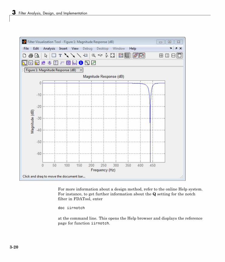
3 Filter Analysis, Design, and Implementation
For more information about a design method, refer to the online Help system.For instance, to get further information about the Q setting for the notchfilter in FDATool, enter
doc iirnotch
at the command line. This opens the Help browser and displays the referencepage for function iirnotch.
3-20
Use FDATool with DSP System Toolbox™ Software
Designing other filters follows a similar procedure, adjusting for differentdesign specification options as each design requires.
Any one of the designs may be quantized in FDATool and analyzed with theavailable analyses on the Analysis menu.
Access the Quantization Features of FDAToolYou use the quantization panel in FDATool to quantize filters. Quantizationrepresents the fourth operating mode for FDATool, along with the filterdesign, filter transformation, and import modes. To switch to quantizationmode, open FDATool from the MATLAB command prompt by entering
fdatool
When FDATool opens, click the Set Quantization Parameters buttonon the side bar. FDATool switches to quantization mode and you see thefollowing panel at the bottom of FDATool, with the default double-precisionoption shown for Filter arithmetic.
3-21
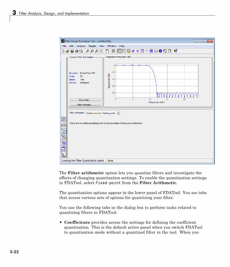
3 Filter Analysis, Design, and Implementation
The Filter arithmetic option lets you quantize filters and investigate theeffects of changing quantization settings. To enable the quantization settingsin FDATool, select Fixed-point from the Filter Arithmetic.
The quantization options appear in the lower panel of FDATool. You see tabsthat access various sets of options for quantizing your filter.
You use the following tabs in the dialog box to perform tasks related toquantizing filters in FDATool:
• Coefficients provides access the settings for defining the coefficientquantization. This is the default active panel when you switch FDAToolto quantization mode without a quantized filter in the tool. When you
3-22
Use FDATool with DSP System Toolbox™ Software
import a fixed-point filter into FDATool, this is the active pane when youswitch to quantization mode.
• Input/Output switches FDATool to the options for quantizing the inputsand outputs for your filter.
• Filter Internals lets you set a variety of options for the arithmetic yourfilter performs, such as how the filter handles the results of multiplicationoperations or how the filter uses the accumulator.
• Apply — applies changes you make to the quantization parameters foryour filter.
Quantize Filters in FDATool
• “Set Quantization Parameters” on page 3-23
• “Coefficients Options” on page 3-24
• “Input/Output Options” on page 3-26
• “Filter Internals Options” on page 3-27
• “Filter Internals Options for CIC Filters” on page 3-30
Set Quantization ParametersQuantized filters have properties that define how they quantize data youfilter. Use the Set Quantization Parameters dialog box in FDATool to setthe properties. Using options in the Set Quantization Parameters dialogbox, FDATool lets you perform a number of tasks:
• Create a quantized filter from a double-precision filter after eitherimporting the filter from your workspace, or using FDATool to design theprototype filter.
• Create a quantized filter that has the default structure (Direct form IItransposed) or any structure you choose, and other property values youselect.
• Change the quantization property values for a quantized filter after youdesign the filter or import it from your workspace.
3-23
3 Filter Analysis, Design, and Implementation
When you click Set Quantization Parameters, and then change Filterarithmetic to Fixed-point, the quantized filter panel opens in FDATool,with the coefficient quantization options set to default values.
Coefficients OptionsTo let you set the properties for the filter coefficients that make up yourquantized filter, FDATool lists options for numerator word length (anddenominator word length if you have an IIR filter). The following table listseach coefficients option and a short description of what the option settingdoes in the filter.
Option Name When Used Description
Numerator Word Length FIR filters only Sets the word length used torepresent numerator coefficients inFIR filters.
Numerator Frac. Length FIR/IIR Sets the fraction length used tointerpret numerator coefficients inFIR filters.
Numerator Range (+/-) FIR/IIR Lets you set the range thenumerators represent. You use thisinstead of the Numerator Frac.Length option to set the precision.When you enter a value x, theresulting range is -x to x. Rangemust be a positive integer.
Coefficient Word Length IIR filters only Sets the word length used torepresent both numerator anddenominator coefficients in IIRfilters. You cannot set differentword lengths for the numerator anddenominator coefficients.
Denominator Frac. Length IIR filters Sets the fraction length used tointerpret denominator coefficientsin IIR filters.
3-24
Use FDATool with DSP System Toolbox™ Software
Option Name When Used Description
Denominator Range (+/-) IIR filters Lets you set the range thedenominator coefficients represent.You use this instead of theDenominator Frac. Lengthoption to set the precision. Whenyou enter a value x, the resultingrange is -x to x. Range must be apositive integer.
Best-precision fractionlengths
All filters Directs FDATool to select thefraction lengths for numerator(and denominator where available)values to maximize the filterperformance. Selecting this optiondisables all of the fraction lengthoptions for the filter.
Scale Values frac. length SOS IIR filters Sets the fraction length used tointerpret the scale values in SOSfilters.
Scale Values range (+/-) SOS IIR filters Lets you set the range the SOSscale values represent. You usethis with SOS filters to adjust thescaling used between filter sections.Setting this value disables theScale Values frac. length option.When you enter a value x, theresulting range is -x to x. Rangemust be a positive integer.
Use unsignedrepresentation
All filters Tells FDATool to interpret thecoefficients as unsigned values.
Scale the numeratorcoefficients to fully utilizethe entire dynamic range
All filters Directs FDATool to scale thenumerator coefficients to effectivelyuse the dynamic range defined bythe numerator word length andfraction length format.
3-25

3 Filter Analysis, Design, and Implementation
Input/Output OptionsThe options that specify how the quantized filter uses input and output valuesare listed in the table below.
Option Name When Used Description
Input Word Length All filters Sets the word length used to representthe input to a filter.
Input fraction length All filters Sets the fraction length used to interpretinput values to filter.
Input range (+/-) All filters Lets you set the range the inputsrepresent. You use this instead of theInput fraction length option to set theprecision. When you enter a value x, theresulting range is -x to x. Range must bea positive integer.
Output word length All filters Sets the word length used to representthe output from a filter.
Avoid overflow All filters Directs the filter to set the fraction lengthfor the input to prevent the output valuesfrom exceeding the available range asdefined by the word length. Clearingthis option lets you set Output fractionlength.
Output fractionlength
All filters Sets the fraction length used to representoutput values from a filter.
Output range (+/-) All filters Lets you set the range the outputsrepresent. You use this instead of theOutput fraction length option to setthe precision. When you enter a valuex, the resulting range is -x to x. Rangemust be a positive integer.
Stage input wordlength
SOS filters only Sets the word length used to representthe input to an SOS filter section.
3-26
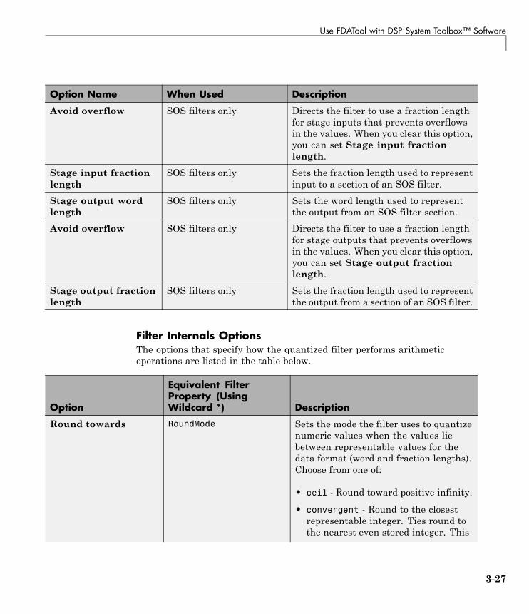
Use FDATool with DSP System Toolbox™ Software
Option Name When Used Description
Avoid overflow SOS filters only Directs the filter to use a fraction lengthfor stage inputs that prevents overflowsin the values. When you clear this option,you can set Stage input fractionlength.
Stage input fractionlength
SOS filters only Sets the fraction length used to representinput to a section of an SOS filter.
Stage output wordlength
SOS filters only Sets the word length used to representthe output from an SOS filter section.
Avoid overflow SOS filters only Directs the filter to use a fraction lengthfor stage outputs that prevents overflowsin the values. When you clear this option,you can set Stage output fractionlength.
Stage output fractionlength
SOS filters only Sets the fraction length used to representthe output from a section of an SOS filter.
Filter Internals OptionsThe options that specify how the quantized filter performs arithmeticoperations are listed in the table below.
Option
Equivalent FilterProperty (UsingWildcard *) Description
Round towards RoundMode Sets the mode the filter uses to quantizenumeric values when the values liebetween representable values for thedata format (word and fraction lengths).Choose from one of:
• ceil - Round toward positive infinity.
• convergent - Round to the closestrepresentable integer. Ties round tothe nearest even stored integer. This
3-27
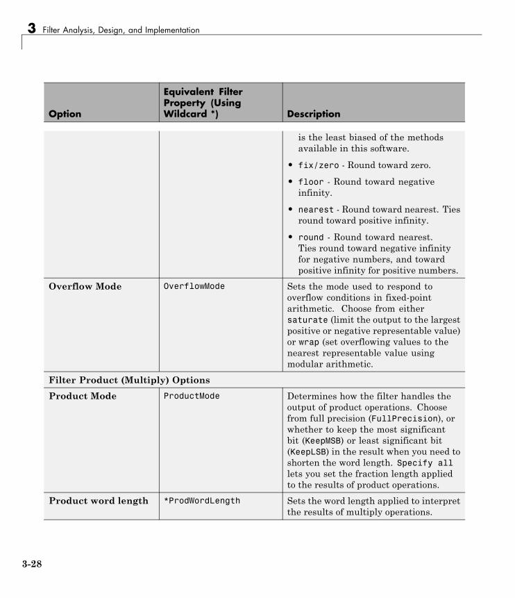
3 Filter Analysis, Design, and Implementation
Option
Equivalent FilterProperty (UsingWildcard *) Description
is the least biased of the methodsavailable in this software.
• fix/zero - Round toward zero.
• floor - Round toward negativeinfinity.
• nearest - Round toward nearest. Tiesround toward positive infinity.
• round - Round toward nearest.Ties round toward negative infinityfor negative numbers, and towardpositive infinity for positive numbers.
Overflow Mode OverflowMode Sets the mode used to respond tooverflow conditions in fixed-pointarithmetic. Choose from eithersaturate (limit the output to the largestpositive or negative representable value)or wrap (set overflowing values to thenearest representable value usingmodular arithmetic.
Filter Product (Multiply) Options
Product Mode ProductMode Determines how the filter handles theoutput of product operations. Choosefrom full precision (FullPrecision), orwhether to keep the most significantbit (KeepMSB) or least significant bit(KeepLSB) in the result when you need toshorten the word length. Specify alllets you set the fraction length appliedto the results of product operations.
Product word length *ProdWordLength Sets the word length applied to interpretthe results of multiply operations.
3-28
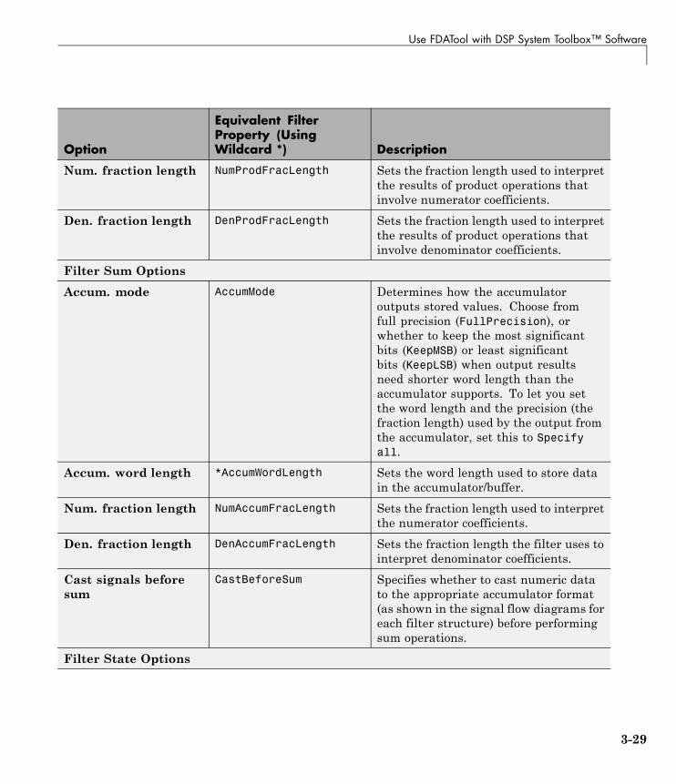
Use FDATool with DSP System Toolbox™ Software
Option
Equivalent FilterProperty (UsingWildcard *) Description
Num. fraction length NumProdFracLength Sets the fraction length used to interpretthe results of product operations thatinvolve numerator coefficients.
Den. fraction length DenProdFracLength Sets the fraction length used to interpretthe results of product operations thatinvolve denominator coefficients.
Filter Sum Options
Accum. mode AccumMode Determines how the accumulatoroutputs stored values. Choose fromfull precision (FullPrecision), orwhether to keep the most significantbits (KeepMSB) or least significantbits (KeepLSB) when output resultsneed shorter word length than theaccumulator supports. To let you setthe word length and the precision (thefraction length) used by the output fromthe accumulator, set this to Specifyall.
Accum. word length *AccumWordLength Sets the word length used to store datain the accumulator/buffer.
Num. fraction length NumAccumFracLength Sets the fraction length used to interpretthe numerator coefficients.
Den. fraction length DenAccumFracLength Sets the fraction length the filter uses tointerpret denominator coefficients.
Cast signals beforesum
CastBeforeSum Specifies whether to cast numeric datato the appropriate accumulator format(as shown in the signal flow diagrams foreach filter structure) before performingsum operations.
Filter State Options
3-29

3 Filter Analysis, Design, and Implementation
Option
Equivalent FilterProperty (UsingWildcard *) Description
State word length *StateWordLength Sets the word length used to representthe filter states. Applied to bothnumerator- and denominator-relatedstates
Avoid overflow None Prevent overflows in arithmeticcalculations by setting the fractionlength appropriately.
State fraction length *StateFracLength Lets you set the fraction lengthapplied to interpret the filter states.Applied to both numerator- anddenominator-related states
Note When you apply changes to the values in the Filter Internals pane, theplots for the Magnitude response estimate and Round-off noise powerspectrum analyses update to reflect those changes. Other types of analysesare not affected by changes to the values in the Filter Internals pane.
Filter Internals Options for CIC FiltersCIC filters use slightly different options for specifying the fixed-pointarithmetic in the filter. The next table shows and describes the options.
Quantize Double-Precision Filters. When you are quantizing adouble-precision filter by switching to fixed-point or single-precision floatingpoint arithmetic, follow these steps.
1 Click Set Quantization Parameters to display the Set QuantizationParameters pane in FDATool.
2 Select Single-precision floating point or Fixed-point from Filterarithmetic.
3-30

Use FDATool with DSP System Toolbox™ Software
When you select one of the optional arithmetic settings, FDATool quantizesthe current filter according to the settings of the options in the SetQuantization Parameter panes, and changes the information displayed inthe analysis area to show quantized filter data.
3 In the quantization panes, set the options for your filter. Set options forCoefficients, Input/Output, and Filter Internals.
4 Click Apply.
FDATool quantizes your filter using your new settings.
5 Use the analysis features in FDATool to determine whether your newquantized filter meets your requirements.
Change the Quantization Properties of Quantized Filters. When youare changing the settings for the quantization of a quantized filter, or afteryou import a quantized filter from your MATLAB workspace, follow thesesteps to set the property values for the filter:
1 Verify that the current filter is quantized.
2 Click Set Quantization Parameters to display the Set QuantizationParameters panel.
3 Review and select property settings for the filter quantization:Coefficients, Input/Output, and Filter Internals. Settings for optionson these panes determine how your filter quantizes data during filteringoperations.
4 Click Apply to update your current quantized filter to use the newquantization property settings from Step 3.
5 Use the analysis features in FDATool to determine whether your newquantized filter meets your requirements.
Analyze Filters with a Noise-Based Method
• “Analyze Filters with the Magnitude Response Estimate Method” on page3-32
3-31

3 Filter Analysis, Design, and Implementation
• “Compare the Estimated and Theoretical Magnitude Responses” on page3-36
• “Select Quantized Filter Structures” on page 3-36
• “Convert the Structure of a Quantized Filter” on page 3-36
• “Convert Filters to Second-Order Sections Form” on page 3-37
Analyze Filters with the Magnitude Response Estimate MethodAfter you design and quantize your filter, the Magnitude ResponseEstimate option on the Analysis menu lets you apply the noise loadingmethod to your filter. When you select Analysis > Magnitude ResponseEstimate from the menu bar, FDATool immediately starts the Monte Carlotrials that form the basis for the method and runs the analysis, ending bydisplaying the results in the analysis area in FDATool.
With the noise-based method, you estimate the complex frequency responsefor your filter as determined by applying a noise- like signal to the filter input.Magnitude Response Estimate uses the Monte Carlo trials to generate anoise signal that contains complete frequency content across the range 0 toFs. The first time you run the analysis, magnitude response estimate usesdefault settings for the various conditions that define the process, such as thenumber of test points and the number of trials.
Analysis ParameterDefaultSetting Description
Number of Points 512 Number of equally spaced pointsaround the upper half of the unitcircle.
Frequency Range 0 to Fs/2 Frequency range of the plotx-axis.
Frequency Units Hz Units for specifying the frequencyrange.
Sampling Frequency 48000 Inverse of the sampling period.
3-32
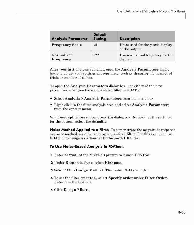
Use FDATool with DSP System Toolbox™ Software
Analysis ParameterDefaultSetting Description
Frequency Scale dB Units used for the y-axis displayof the output.
NormalizedFrequency
Off Use normalized frequency for thedisplay.
After your first analysis run ends, open the Analysis Parameters dialogbox and adjust your settings appropriately, such as changing the number oftrials or number of points.
To open the Analysis Parameters dialog box, use either of the nextprocedures when you have a quantized filter in FDATool:
• Select Analysis > Analysis Parameters from the menu bar
• Right-click in the filter analysis area and select Analysis Parametersfrom the context menu
Whichever option you choose opens the dialog box. Notice that the settingsfor the options reflect the defaults.
Noise Method Applied to a Filter. To demonstrate the magnitude responseestimate method, start by creating a quantized filter. For this example, useFDATool to design a sixth-order Butterworth IIR filter.
To Use Noise-Based Analysis in FDATool.
1 Enter fdatool at the MATLAB prompt to launch FDATool.
2 Under Response Type, select Highpass.
3 Select IIR in Design Method. Then select Butterworth.
4 To set the filter order to 6, select Specify order under Filter Order.Enter 6 in the text box.
5 Click Design Filter.
3-33
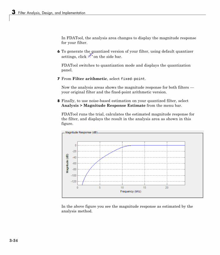
3 Filter Analysis, Design, and Implementation
In FDATool, the analysis area changes to display the magnitude responsefor your filter.
6 To generate the quantized version of your filter, using default quantizersettings, click on the side bar.
FDATool switches to quantization mode and displays the quantizationpanel.
7 From Filter arithmetic, select fixed-point.
Now the analysis areas shows the magnitude response for both filters —your original filter and the fixed-point arithmetic version.
8 Finally, to use noise-based estimation on your quantized filter, selectAnalysis > Magnitude Response Estimate from the menu bar.
FDATool runs the trial, calculates the estimated magnitude response forthe filter, and displays the result in the analysis area as shown in thisfigure.
In the above figure you see the magnitude response as estimated by theanalysis method.
3-34

Use FDATool with DSP System Toolbox™ Software
View the Noise Power Spectrum. When you use the noise method toestimate the magnitude response of a filter, FDATool simulates and appliesa spectrum of noise values to test your filter response. While the simulatednoise is essentially white, you might want to see the actual spectrum thatFDATool used to test your filter.
From the Analysis menu bar option, select Round-off Noise PowerSpectrum. In the analysis area in FDATool, you see the spectrum of thenoise used to estimate the filter response. The details of the noise spectrum,such as the range and number of data points, appear in the AnalysisParameters dialog box.
For more information, refer to McClellan, et al., Computer-Based Exercisesfor Signal Processing Using MATLAB 5, Prentice-Hall, 1998. See Project 5:Quantization Noise in Digital Filters, page 231.
Change Your Noise Analysis Parameters. In “Noise Method Appliedto a Filter” on page 3-33, you used synthetic white noise to estimate themagnitude response for a fixed-point highpass Butterworth filter. Since youran the estimate only once in FDATool, your noise analysis used the defaultanalysis parameters settings shown in “Analyze Filters with the MagnitudeResponse Estimate Method” on page 3-32.
To change the settings, follow these steps after the first time you use thenoise estimate on your quantized filter.
1 With the results from running the noise estimating method displayed inthe FDATool analysis area, select Analysis > Analysis Parametersfrom the menu bar.
To give you access to the analysis parameters, the Analysis Parametersdialog box opens (with default settings).
2 To use more points in the spectrum to estimate the magnitude response,change Number of Points to 1024 and click OK to run the analysis.
FDATool closes the Analysis Parameters dialog box and reruns the noiseestimate, returning the results in the analysis area.
To rerun the test without closing the dialog box, press Enter after you typeyour new value into a setting, then click Apply. Now FDATool runs the
3-35
3 Filter Analysis, Design, and Implementation
test without closing the dialog box. When you want to try many differentsettings for the noise-based analysis, this is a useful shortcut.
Compare the Estimated and Theoretical Magnitude ResponsesAn important measure of the effectiveness of the noise method for estimatingthe magnitude response of a quantized filter is to compare the estimatedresponse to the theoretical response.
One way to do this comparison is to overlay the theoretical response on theestimated response. While you have the Magnitude Response Estimatedisplaying in FDATool, select Analysis > Overlay Analysis from the menubar. Then selectMagnitude Response to show both response curves plottedtogether in the analysis area.
Select Quantized Filter StructuresFDATool lets you change the structure of any quantized filter. Use theConvert structure option to change the structure of your filter to one thatmeets your needs.
To learn about changing the structure of a filter in FDATool, refer to“Converting the Filter Structure” on page 13-23 in your Signal ProcessingToolbox documentation.
Convert the Structure of a Quantized FilterYou use the Convert structure option to change the structure of filter. Whenthe Source is Designed(Quantized) or Imported(Quantized), Convertstructure lets you recast the filter to one of the following structures:
• “Direct Form II Transposed Filter Structure”
• “Direct Form I Transposed Filter Structure”
• “Direct Form II Filter Structure”
• “Direct Form I Filter Structure”
• “Direct Form Finite Impulse Response (FIR) Filter Structure”
• “Direct Form FIR Transposed Filter Structure”
• “Lattice Autoregressive Moving Average (ARMA) Filter Structure”
3-36

Use FDATool with DSP System Toolbox™ Software
• dfilt.calattice
• dfilt.calatticepc
• “Direct Form Antisymmetric FIR Filter Structure (Any Order)”
Starting from any quantized filter, you can convert to one of the followingrepresentation:
• Direct form I
• Direct form II
• Direct form I transposed
• Direct form II transposed
• Lattice ARMA
Additionally, FDATool lets you do the following conversions:
• Minimum phase FIR filter to Lattice MA minimum phase
• Maximum phase FIR filter to Lattice MA maximum phase
• Allpass filters to Lattice allpass
Refer to “FilterStructure” for details about each of these structures.
Convert Filters to Second-Order Sections FormTo learn about using FDATool to convert your quantized filter to usesecond-order sections, refer to “Converting to Second-Order Sections” on page13-25 in your Signal Processing Toolbox documentation. You might noticethat filters you design in FDATool, rather than filters you imported, areimplemented in SOS form.
View Filter Structures in FDATool. To open the demonstration, clickHelp > Show filter structures. After the Help browser opens, you see thereference page for the current filter. You find the filter structure signal flowdiagram on this reference page, or you can navigate to reference pages forother filter.
3-37

3 Filter Analysis, Design, and Implementation
Scale Second-Order Section Filters
• “Use the Reordering and Scaling Second-Order Sections Dialog Box” onpage 3-38
• “Scale an SOS Filter” on page 3-40
Use the Reordering and Scaling Second-Order Sections DialogBoxFDATool provides the ability to scale SOS filters after you create them. Usingoptions on the Reordering and Scaling Second-Order Sections dialog box,FDATool scales either or both the filter numerators and filter scale valuesaccording to your choices for the scaling options.
3-38
Use FDATool with DSP System Toolbox™ Software
Parameter Description and Valid Value
Scale Apply any scaling options to the filter. Select thiswhen you are reordering your SOS filter and youwant to scale it at the same time. Or when youare scaling your filter, with or without reordering.Scaling is disabled by default.
No Overflow — HighSNR slider
Lets you set whether scaling favors reducingarithmetic overflow in the filter or maximizingthe signal-to-noise ratio (SNR) at the filteroutput. Moving the slider to the right increasesthe emphasis on SNR at the expense of possibleoverflows. The markings indicate the P-normapplied to achieve the desired result in SNR oroverflow protection. For more information aboutthe P-norm settings, refer to norm for details.
MaximumNumerator
Maximum allowed value for numeratorcoefficients after scaling.
NumeratorConstraint
Specifies whether and how to constrainnumerator coefficient values. Options are none,normalize, power of 2, and unit. Choosingnone lets the scaling use any scale value forthe numerators by removing any constraintson the numerators, except that the coefficientswill be clipped if they exceed the MaximumNumerator. With Normalize the maximumabsolute value of the numerator is forced to equalthe Maximum Numerator value (for all otherconstraints, the Maximum Numerator is onlyan upper limit, above which coefficients will beclipped). The power of 2 option forces scaling touse numerator values that are powers of 2, suchas 2 or 0.5. With unit, the leading coefficient ofeach numerator is forced to a value of 1.
3-39

3 Filter Analysis, Design, and Implementation
Parameter Description and Valid Value
Overflow Mode Sets the way the filter handles arithmeticoverflow situations during scaling. Choosefrom either saturate (limit the output to thelargest positive or negative representable value)or wrap (set overflowing values to the nearestrepresentable value using modular arithmetic.
Scale ValueConstraint
Specify whether to constrain the filter scalevalues, and how to constrain them. Valid optionsare unit, power of 2, and none. Choosing unitfor the constraint disables the Max. ScaleValue setting and forces scale values to equal1. Power of 2 constrains the scale values to bepowers of 2, such as 2 or 0.5, while none removesany constraint on the scale values, except thatthey cannot exceed theMax. Scale Value.
Max. Scale Value Sets the maximum allowed scale values. SOSfilter scaling applies theMax. Scale Value limitonly when you set Scale Value Constraint toa value other than unit (the default setting).Setting a maximum scale value removes anyother limits on the scale values.
Revert to OriginalFilter
Returns your filter to the original scaling. Beingable to revert to your original filter makes iteasier to assess the results of scaling your filter.
Various combinations of settings let you scale filter numerators withoutchanging the scale values, or adjust the filter scale values without changingthe numerators. There is no scaling control for denominators.
Scale an SOS FilterStart the process by designing a lowpass elliptical filter in FDATool.
1 Launch FDATool.
2 In Response Type, select Lowpass.
3-40

Use FDATool with DSP System Toolbox™ Software
3 In Design Method, select IIR and Elliptic from the IIR design methodslist.
4 Select Minimum Order for the filter.
5 Switch the frequency units by choosing Normalized(0 to 1) from theUnits list.
6 To set the passband specifications, enter 0.45 for wpass and 0.55 forwstop. Finally, inMagnitude Specifications, set Astop to 60.
7 Click Design Filter to design the filter.
After FDATool finishes designing the filter, you see the following plot andsettings in the tool.
3-41

3 Filter Analysis, Design, and Implementation
You kept the Options setting for Match exactly as both, meaning thefilter design matches the specification for the passband and the stopband.
8 To switch to scaling the filter, select Edit > Reorder and ScaleSecond-Order Sections from the menu bar.
9 To see the filter coefficients, return to FDATool and select FilterCoefficients from the Analysis menu. FDATool displays the coefficientsand scale values in FDATool.
With the coefficients displayed you can see the effects of scaling your filterdirectly in the scale values and filter coefficients.
3-42
Use FDATool with DSP System Toolbox™ Software
Now try scaling the filter in a few different ways. First scale the filter tomaximize the SNR.
1 Return to the Reordering and Scaling Second-Order Sections dialogbox and select None for Reordering in the left pane. This preventsFDATool from reordering the filter sections when you rescale the filter.
2 Move the No Overflow—High SNR slider from No Overflow to HighSNR.
3 Click Apply to scale the filter and leave the dialog box open.
After a few moments, FDATool updates the coefficients displayed so yousee the new scaling.
All of the scale factors are now 1, and the SOS matrix of coefficients showsthat none of the numerator coefficients are 1 and the first denominatorcoefficient of each section is 1.
4 Click Revert to Original Filter to restore the filter to the originalsettings for scaling and coefficients.
Reorder the Sections of Second-Order Section Filters
Reorder Filters Using FDAToolFDATool designs most discrete-time filters in second-order sections.Generally, SOS filters resist the effects of quantization changes when youcreate fixed-point filters. After you have a second-order section filter inFDATool, either one you designed in the tool, or one you imported, FDAToolprovides the capability to change the order of the sections that compose thefilter. Any SOS filter in FDATool allows reordering of the sections.
To reorder the sections of a filter, you access the Reorder and Scaling ofSecond-Order Sections dialog box in FDATool.
With your SOS filter in FDATool, select Edit > Reorder and Scale fromthe menu bar. FDATool returns the reordering dialog box shown here withthe default settings.
3-43

3 Filter Analysis, Design, and Implementation
Controls on the Reordering and Scaling of Second-Order Sections dialog box
In this dialog box, the left-hand side contains options for reordering SOSfilters. On the right you see the scaling options. These are independent —reordering your filter does not require scaling (note the Scale option) andscaling does not require that you reorder your filter (note the None optionunder Reordering). For more about scaling SOS filters, refer to “ScaleSecond-Order Section Filters” on page 3-38 and to scale in the referencesection.
Reordering SOS filters involves using the options in the Reordering andScaling of Second-Order Sections dialog box. The following table listseach reorder option and provides a description of what the option does.
3-44

Use FDATool with DSP System Toolbox™ Software
Control Option Description
Auto Reorders the filter sections to minimize the outputnoise power of the filter. Note that differentordering applies to each specification type, such aslowpass or highpass. Automatic ordering adapts tothe specification type of your filter.
None Does no reordering on your filter. SelectingNone lets you scale your filter without applyingreordering at the same time. When you access thisdialog box with a current filter, this is the defaultsetting — no reordering is applied.
Least selectivesection to mostselective section
Rearranges the filter sections so the leastrestrictive (lowest Q) section is the first sectionand the most restrictive (highest Q) section is thelast section.
Most selectivesection to leastselective section
Rearranges the filter sections so the mostrestrictive (highest Q) section is the first sectionand the least restrictive (lowest Q) section is thelast section.
Custom reordering Lets you specify the section ordering to use byenabling the Numerator Order and DenominatorOrder options
Numerator Order Specify new ordering for the sections of your SOSfilter. Enter a vector of the indices of the sectionsin the order in which to rearrange them. Forexample, a filter with five sections has indices 1,2, 3, 4, and 5. To switch the second and fourthsections, the vector would be [1,4,3,2,5].
Use NumeratorOrder
Rearranges the denominators in the order assignedto the numerators.
3-45
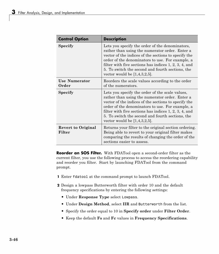
3 Filter Analysis, Design, and Implementation
Control Option Description
Specify Lets you specify the order of the denominators,rather than using the numerator order. Enter avector of the indices of the sections to specify theorder of the denominators to use. For example, afilter with five sections has indices 1, 2, 3, 4, and5. To switch the second and fourth sections, thevector would be [1,4,3,2,5].
Use NumeratorOrder
Reorders the scale values according to the orderof the numerators.
Specify Lets you specify the order of the scale values,rather than using the numerator order. Enter avector of the indices of the sections to specify theorder of the denominators to use. For example, afilter with five sections has indices 1, 2, 3, 4, and5. To switch the second and fourth sections, thevector would be [1,4,3,2,5].
Revert to OriginalFilter
Returns your filter to the original section ordering.Being able to revert to your original filter makescomparing the results of changing the order of thesections easier to assess.
Reorder an SOS Filter. With FDATool open a second-order filter as thecurrent filter, you use the following process to access the reordering capabilityand reorder you filter. Start by launching FDATool from the commandprompt.
1 Enter fdatool at the command prompt to launch FDATool.
2 Design a lowpass Butterworth filter with order 10 and the defaultfrequency specifications by entering the following settings:
• Under Response Type select Lowpass.
• Under Design Method, select IIR and Butterworth from the list.
• Specify the order equal to 10 in Specify order under Filter Order.
• Keep the default Fs and Fc values in Frequency Specifications.
3-46

Use FDATool with DSP System Toolbox™ Software
3 Click Design Filter.
FDATool designs the Butterworth filter and returns your filter as aDirect-Form II filter implemented with second-order sections. You see thespecifications in the Current Filter Information area.
With the second-order filter in FDATool, reordering the filter uses theReordering and Scaling of Second-Order Sections feature in FDATool(also available in Filter Visualization Tool, fvtool).
4 To reorder your filter, select Edit > Reorder and Scale Second-OrderSections from the FDATool menus.
Now you are ready to reorder the sections of your filter. Note that FDAToolperforms the reordering on the current filter in the session.
Use Least Selective to Most Selective Section Reordering. To letFDATool reorder your filter so the least selective section is first and the mostselective section is last, perform the following steps in the Reordering andScaling of Second-Order Sections dialog box.
1 In Reordering, select Least selective section to most selectivesection.
2 To prevent filter scaling at the same time, clear Scale in Scaling.
3 In FDATool, select View > SOS View Settings from the menu bar so yousee the sections of your filter displayed in FDATool.
4 In the SOS View Settings dialog box, select Individual sections.Making this choice configures FDATool to show the magnitude responsecurves for each section of your filter in the analysis area.
5 Back in the Reordering and Scaling of Second-Order Sections dialogbox, click Apply to reorder your filter according to the Qs of the filtersections, and keep the dialog box open. In response, FDATool presentsthe responses for each filter section (there should be five sections) in theanalysis area.
3-47
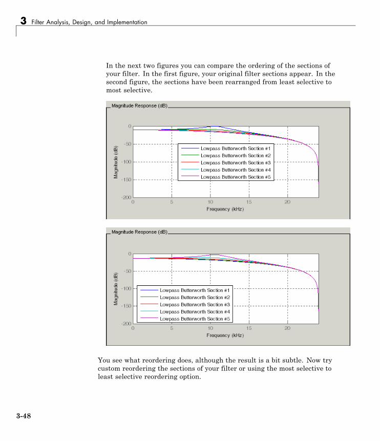
3 Filter Analysis, Design, and Implementation
In the next two figures you can compare the ordering of the sections ofyour filter. In the first figure, your original filter sections appear. In thesecond figure, the sections have been rearranged from least selective tomost selective.
You see what reordering does, although the result is a bit subtle. Now trycustom reordering the sections of your filter or using the most selective toleast selective reordering option.
3-48

Use FDATool with DSP System Toolbox™ Software
View SOS Filter Sections
• “Using the SOS View Dialog Box” on page 3-49
• “View the Sections of SOS Filters” on page 3-51
Using the SOS View Dialog BoxSince you can design and reorder the sections of SOS filters, FDATool providesthe ability to view the filter sections in the analysis area — SOS View. Onceyou have a second-order section filter as your current filter in FDATool,you turn on the SOS View option to see the filter sections individually, orcumulatively, or even only some of the sections. Enabling SOS View putsFDATool in a mode where all second-order section filters display sections untilyou disable the SOS View option. SOS View mode applies to any analysis youdisplay in the analysis area. For example, if you configure FDATool to showthe phase responses for filters, enabling SOS View means FDATool displaysthe phase response for each section of SOS filters.
Controls on the SOS View Dialog Box
SOS View uses a few options to control how FDATool displays the sections,or which sections to display. When you select View > SOS View from theFDATool menu bar, you see this dialog box containing options to configureSOS View operation.
3-49
3 Filter Analysis, Design, and Implementation
By default, SOS View shows the overall response of SOS filters. Options inthe SOS View dialog box let you change the display. This table lists all theoptions and describes the effects of each.
Option Description
Overall Filter This is the familiar display in FDATool. Fora second-order section filter you see only theoverall response rather than the responses forthe individual sections. This is the defaultconfiguration.
Individual sections When you select this option, FDATool displaysthe response for each section as a curve.If your filter has five sections you see fiveresponse curves, one for each section, and theyare independent. Compare to Cumulativesections.
Cumulative sections When you select this option, FDATooldisplays the response for each section as theaccumulated response of all prior sections inthe filter. If your filter has five sections yousee five response curves:
• The first curve plots the response for thefirst filter section.
• The second curve plots the response for thecombined first and second sections.
• The third curve plots the response for thefirst, second, and third sections combined.
And so on until all filter sections appear in thedisplay. The final curve represents the overallfilter response. Compare to Cumulativesections and Overall Filter.
3-50

Use FDATool with DSP System Toolbox™ Software
Option Description
User defined Here you define which sections to display, andin which order. Selecting this option enablesthe text box where you enter a cell array ofthe indices of the filter sections. Each indexrepresents one section. Entering one indexplots one response. Entering something like{1:2} plots the combined response of sections 1and 2. If you have a filter with four sections,the entry {1:4} plots the combined response forall four sections, whereas {1,2,3,4} plots theresponse for each section. Note that after youenter the cell array, you need to click OK orApply to update the FDATool analysis area tothe new SOS View configuration.
Use secondary-scalingpoints
This directs FDATool to use the secondaryscaling points in the sections to determinewhere to split the sections. This option appliesonly when the filter is a df2sos or df1tsosfilter. For these structures, the secondaryscaling points refer to the scaling locationsbetween the recursive and the nonrecursiveparts of the section (the "middle" of the section).By default, secondary-scaling points is notenabled. You use this with the Cumulativesections option only.
View the Sections of SOS FiltersAfter you design or import an SOS filter in to FDATool, the SOS view optionlets you see the per section performance of your filter. Enabling SOS Viewfrom the View menu in FDATool configures the tool to display the sections ofSOS filters whenever the current filter is an SOS filter.
These next steps demonstrate using SOS View to see your filter sectionsdisplayed in FDATool.
1 Launch FDATool.
3-51
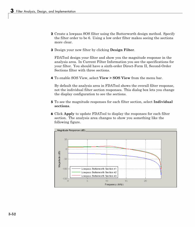
3 Filter Analysis, Design, and Implementation
2 Create a lowpass SOS filter using the Butterworth design method. Specifythe filter order to be 6. Using a low order filter makes seeing the sectionsmore clear.
3 Design your new filter by clicking Design Filter.
FDATool design your filter and show you the magnitude response in theanalysis area. In Current Filter Information you see the specifications foryour filter. You should have a sixth-order Direct-Form II, Second-OrderSections filter with three sections.
4 To enable SOS View, select View > SOS View from the menu bar.
By default the analysis area in FDATool shows the overall filter response,not the individual filter section responses. This dialog box lets you changethe display configuration to see the sections.
5 To see the magnitude responses for each filter section, select Individualsections.
6 Click Apply to update FDATool to display the responses for each filtersection. The analysis area changes to show you something like thefollowing figure.
3-52

Use FDATool with DSP System Toolbox™ Software
If you switch FDATool to display filter phase responses (by selectingAnalysis > Phase Response), you see the phase response for each filtersection in the analysis area.
7 To define your own display of the sections, you use the User definedoption and enter a vector of section indices to display. Now you see adisplay of the first section response, and the cumulative first, second, andthird sections response:
• Select User defined to enable the text entry box in the dialog box.
• Enter the cell array {1,1:3} to specify that FDATool should display theresponse of the first section and the cumulative response of the firstthree sections of the filter.
8 To apply your new SOS View selection, click Apply or OK (which closesthe SOS View dialog box).
In the FDATool analysis area you see two curves — one for the responseof the first filter section and one for the combined response of sections1, 2, and 3.
3-53
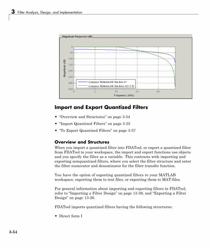
3 Filter Analysis, Design, and Implementation
Import and Export Quantized Filters
• “Overview and Structures” on page 3-54
• “Import Quantized Filters” on page 3-55
• “To Export Quantized Filters” on page 3-57
Overview and StructuresWhen you import a quantized filter into FDATool, or export a quantized filterfrom FDATool to your workspace, the import and export functions use objectsand you specify the filter as a variable. This contrasts with importing andexporting nonquantized filters, where you select the filter structure and enterthe filter numerator and denominator for the filter transfer function.
You have the option of exporting quantized filters to your MATLABworkspace, exporting them to text files, or exporting them to MAT-files.
For general information about importing and exporting filters in FDATool,refer to “Importing a Filter Design” on page 13-39, and “Exporting a FilterDesign” on page 13-26.
FDATool imports quantized filters having the following structures:
• Direct form I
3-54

Use FDATool with DSP System Toolbox™ Software
• Direct form II
• Direct form I transposed
• Direct form II transposed
• Direct form symmetric FIR
• Direct form antisymmetric FIR
• Lattice allpass
• Lattice AR
• Lattice MA minimum phase
• Lattice MA maximum phase
• Lattice ARMA
• Lattice coupled-allpass
• Lattice coupled-allpass power complementary
Import Quantized FiltersAfter you design or open a quantized filter in your MATLAB workspace,FDATool lets you import the filter for analysis. Follow these steps to importyour filter in to FDATool:
1 Open FDATool.
2 Select File > Import Filter from Workspace from the menu bar, orchoose the Import Filter from Workspace icon in the side panel:
.
In the lower region of FDATool, the Design Filter pane becomes ImportFilter, and options appear for importing quantized filters, as shown.
3-55
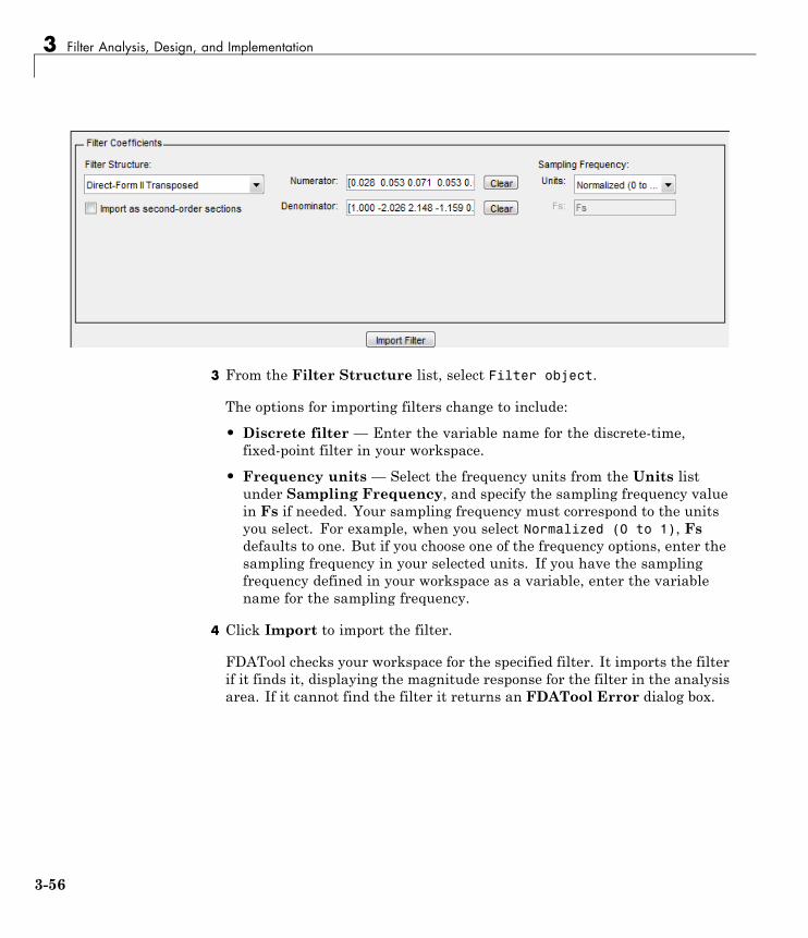
3 Filter Analysis, Design, and Implementation
3 From the Filter Structure list, select Filter object.
The options for importing filters change to include:
• Discrete filter — Enter the variable name for the discrete-time,fixed-point filter in your workspace.
• Frequency units — Select the frequency units from the Units listunder Sampling Frequency, and specify the sampling frequency valuein Fs if needed. Your sampling frequency must correspond to the unitsyou select. For example, when you select Normalized (0 to 1), Fsdefaults to one. But if you choose one of the frequency options, enter thesampling frequency in your selected units. If you have the samplingfrequency defined in your workspace as a variable, enter the variablename for the sampling frequency.
4 Click Import to import the filter.
FDATool checks your workspace for the specified filter. It imports the filterif it finds it, displaying the magnitude response for the filter in the analysisarea. If it cannot find the filter it returns an FDATool Error dialog box.
3-56
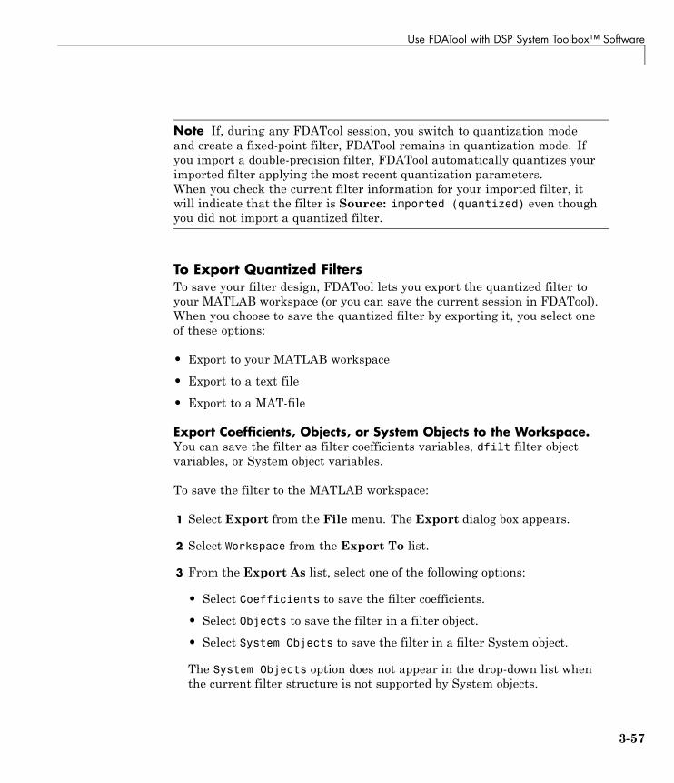
Use FDATool with DSP System Toolbox™ Software
Note If, during any FDATool session, you switch to quantization modeand create a fixed-point filter, FDATool remains in quantization mode. Ifyou import a double-precision filter, FDATool automatically quantizes yourimported filter applying the most recent quantization parameters.When you check the current filter information for your imported filter, itwill indicate that the filter is Source: imported (quantized) even thoughyou did not import a quantized filter.
To Export Quantized FiltersTo save your filter design, FDATool lets you export the quantized filter toyour MATLAB workspace (or you can save the current session in FDATool).When you choose to save the quantized filter by exporting it, you select oneof these options:
• Export to your MATLAB workspace
• Export to a text file
• Export to a MAT-file
Export Coefficients, Objects, or System Objects to the Workspace.You can save the filter as filter coefficients variables, dfilt filter objectvariables, or System object variables.
To save the filter to the MATLAB workspace:
1 Select Export from the File menu. The Export dialog box appears.
2 Select Workspace from the Export To list.
3 From the Export As list, select one of the following options:
• Select Coefficients to save the filter coefficients.
• Select Objects to save the filter in a filter object.
• Select System Objects to save the filter in a filter System object.
The System Objects option does not appear in the drop-down list whenthe current filter structure is not supported by System objects.
3-57
3 Filter Analysis, Design, and Implementation
4 Assign a variable name:
• For coefficients, assign variable names using the Numerator andDenominator options under Variable Names.
• For objects or System objects, assign the variable name in the DiscreteFilter option.
If you have variables with the same names in your workspace and you wantto overwrite them, select the Overwrite Variables box.
5 Click Export.
Do not try to export the filter to a variable name that exists in yourworkspace without selecting Overwrite existing variables, in theprevious step. If you do so, FDATool stops the export operation. The toolreturns a warning that the variable you specified as the quantized filtername already exists in the workspace.
• To continue to export the filter to the existing variable, click OK todismiss the warning.
• Then select the Overwrite existing variables check box and clickExport.
Getting Filter Coefficients After Exporting. To extract the filtercoefficients from your quantized filter after you export the filter to MATLAB,use the celldisp function in MATLAB. For example, create a quantized filterin FDATool, and export the filter as Hq. To extract the filter coefficients forHq, use
celldisp(Hq.referencecoefficients)
which returns the cell array containing the filter reference coefficients, or
celldisp(Hq.quantizedcoefficients
to return the quantized coefficients.
Export Filter Coefficients as a Text File. To save your quantized filter as atext file, follow these steps:
1 Select Export from the File menu.
3-58
Use FDATool with DSP System Toolbox™ Software
2 Select Text-file under Export to.
3 Click OK to export the filter and close the dialog box. Click Apply to exportthe filter without closing the Export dialog box. Clicking Apply letsyou export your quantized filter to more than one name without leavingthe Export dialog box.
The Export Filter Coefficients to Text-file dialog box appears. This isthe standard Microsoft Windows® save file dialog box.
4 Choose or enter a folder and filename for the text file, and click OK.
FDATool exports your quantized filter as a text file with the name youprovided, and the MATLAB editor opens, displaying the file for editing.
Export Filter Coefficients as a MAT-File. To save your quantized filter as aMAT-file, follow these steps:
1 Select Export from the File menu.
2 Select MAT-file under Export to.
3 Assign a variable name for the filter.
4 Click OK to export the filter and close the dialog box. Click Apply to exportthe filter without closing the Export dialog box. Clicking Apply letsyou export your quantized filter to more than one name without leavingthe Export dialog box.
The Export Filter Coefficients to MAT-file dialog box appears. Thisdialog box is the standard Microsoft Windows save file dialog box.
5 Choose or enter a folder and filename for the text file, and click OK.
FDATool exports your quantized filter as a MAT-file with the specifiedname.
Generate MATLAB CodeYou can generate MATLAB code using the File > Generate MATLAB Codemenu. This menu has three options:
3-59

3 Filter Analysis, Design, and Implementation
• Filter Design Function
This option creates MATLAB code that generates the DFILT/MFILT objectcurrently designed in FDATool.
• Filter Design Function (with System Objects)
This option is similar to the previous option with the difference that aSystem object is generated instead of a DFILT/MFILT object. The option isdisabled when the current filter is not supported by system objects.
• Data Filtering Function (with System Objects)
This option generates MATLAB code that filters input data with thecurrent filter design. The MATLAB code is ready to be converted to C/C++code using the codegen command. This option is disabled when the currentfilter is not supported by system objects.
Import XILINX Coefficient (.COE) Files
Import XILINX .COE Files into FDAToolYou can import XILINX coefficients (.coe) files into FDATool to createquantized filters directly using the imported filter coefficients.
To use the import file feature:
1 Select File > Import Filter From XILINX Coefficient (.COE) Filein FDATool.
2 In the Import Filter From XILINX Coefficient (.COE) File dialog box,find and select the .coe file to import.
3 Click Open to dismiss the dialog box and start the import process.
FDATool imports the coefficient file and creates a quantized, single-section,direct-form FIR filter.
Transform Filters Using FDATool
• “Filter Transformation Capabilities of FDATool” on page 3-61
• “Original Filter Type” on page 3-62
3-60
Use FDATool with DSP System Toolbox™ Software
• “Frequency Point to Transform” on page 3-66
• “Transformed Filter Type” on page 3-66
• “Specify Desired Frequency Location” on page 3-67
Filter Transformation Capabilities of FDAToolThe toolbox provides functions for transforming filters between various forms.When you use FDATool with the toolbox installed, a side bar button and amenu bar option enable you to use the Transform Filter panel to transformfilters as well as using the command line functions.
From the selection on the FDATool menu bar — Transformations — youcan transform lowpass FIR and IIR filters to a variety of passband shapes.
You can convert your FIR filters from:
• Lowpass to lowpass.
• Lowpass to highpass.
For IIR filters, you can convert from:
• Lowpass to lowpass.
• Lowpass to highpass.
• Lowpass to bandpass.
• Lowpass to bandstop.
When you click the Transform Filter button, , on the side bar, theTransform Filter panel opens in FDATool, as shown here.
3-61
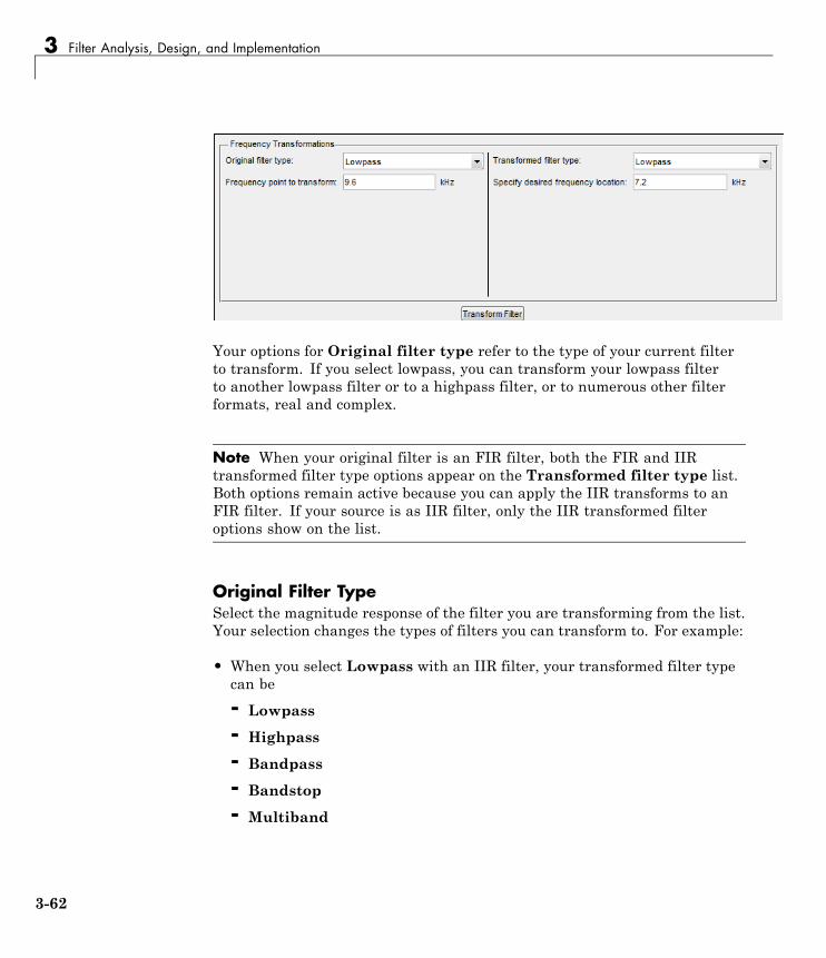
3 Filter Analysis, Design, and Implementation
Your options for Original filter type refer to the type of your current filterto transform. If you select lowpass, you can transform your lowpass filterto another lowpass filter or to a highpass filter, or to numerous other filterformats, real and complex.
Note When your original filter is an FIR filter, both the FIR and IIRtransformed filter type options appear on the Transformed filter type list.Both options remain active because you can apply the IIR transforms to anFIR filter. If your source is as IIR filter, only the IIR transformed filteroptions show on the list.
Original Filter TypeSelect the magnitude response of the filter you are transforming from the list.Your selection changes the types of filters you can transform to. For example:
• When you select Lowpass with an IIR filter, your transformed filter typecan be
- Lowpass
- Highpass
- Bandpass
- Bandstop
- Multiband
3-62

Use FDATool with DSP System Toolbox™ Software
- Bandpass (complex)
- Bandstop (complex)
- Multiband (complex)
• When you select Lowpass with an FIR filter, your transformed filtertype can be
- Lowpass
- Lowpass (FIR)
- Highpass
- Highpass (FIR) narrowband
- Highpass (FIR) wideband
- Bandpass
- Bandstop
- Multiband
- Bandpass (complex)
- Bandstop (complex)
- Multiband (complex)
In the following table you see each available original filter type and all thetypes of filter to which you can transform your original.
Original Filter Available Transformed Filter Types
Lowpass FIR • Lowpass
• Lowpass (FIR)
• Highpass
• Highpass (FIR) narrowband
• Highpass (FIR) wideband
• Bandpass
• Bandstop
• Multiband
3-63

3 Filter Analysis, Design, and Implementation
Original Filter Available Transformed Filter Types
• Bandpass (complex)
• Bandstop (complex)
• Multiband (complex)
Lowpass IIR • Lowpass
• Highpass
• Bandpass
• Bandstop
• Multiband
• Bandpass (complex)
• Bandstop (complex)
• Multiband (complex)
Highpass FIR • Lowpass
• Lowpass (FIR) narrowband
• Lowpass (FIR) wideband
• Highpass (FIR)
• Highpass
• Bandpass
• Bandstop
• Multiband
• Bandpass (complex)
• Bandstop (complex)
• Multiband (complex)
3-64
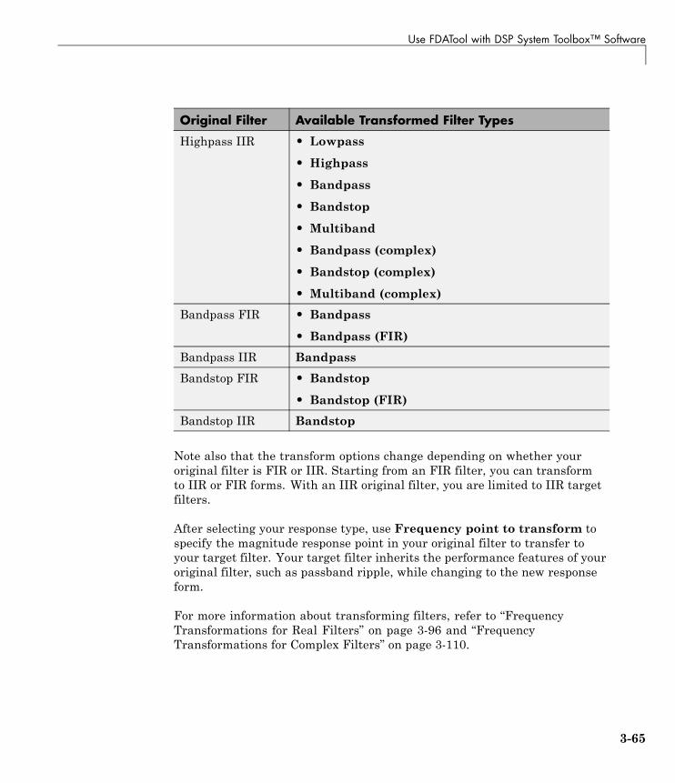
Use FDATool with DSP System Toolbox™ Software
Original Filter Available Transformed Filter Types
Highpass IIR • Lowpass
• Highpass
• Bandpass
• Bandstop
• Multiband
• Bandpass (complex)
• Bandstop (complex)
• Multiband (complex)
Bandpass FIR • Bandpass
• Bandpass (FIR)
Bandpass IIR Bandpass
Bandstop FIR • Bandstop
• Bandstop (FIR)
Bandstop IIR Bandstop
Note also that the transform options change depending on whether youroriginal filter is FIR or IIR. Starting from an FIR filter, you can transformto IIR or FIR forms. With an IIR original filter, you are limited to IIR targetfilters.
After selecting your response type, use Frequency point to transform tospecify the magnitude response point in your original filter to transfer toyour target filter. Your target filter inherits the performance features of youroriginal filter, such as passband ripple, while changing to the new responseform.
For more information about transforming filters, refer to “FrequencyTransformations for Real Filters” on page 3-96 and “FrequencyTransformations for Complex Filters” on page 3-110.
3-65

3 Filter Analysis, Design, and Implementation
Frequency Point to TransformThe frequency point you enter in this field identifies a magnitude responsevalue (in dB) on the magnitude response curve.
When you enter frequency values in the Specify desired frequencylocation option, the frequency transformation tries to set the magnituderesponse of the transformed filter to the value identified by the frequencypoint you enter in this field.
While you can enter any location, generally you should specify a filterpassband or stopband edge, or a value in the passband or stopband.
The Frequency point to transform sets the magnitude response at thevalues you enter in Specify desired frequency location. Specify a valuethat lies at either the edge of the stopband or the edge of the passband.
If, for example, you are creating a bandpass filter from a highpass filter, thetransformation algorithm sets the magnitude response of the transformedfilter at the Specify desired frequency location to be the same as theresponse at the Frequency point to transform value. Thus you get abandpass filter whose response at the low and high frequency locations is thesame. Notice that the passband between them is undefined. In the next twofigures you see the original highpass filter and the transformed bandpassfilter.
For more information about transforming filters, refer to “Digital FrequencyTransformations” on page 3-88.
Transformed Filter TypeSelect the magnitude response for the target filter from the list. The completelist of transformed filter types is:
• Lowpass
• Lowpass (FIR)
• Highpass
• Highpass (FIR) narrowband
• Highpass (FIR) wideband
3-66
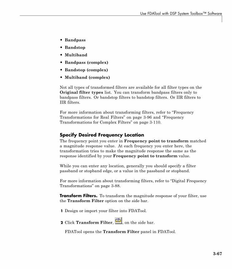
Use FDATool with DSP System Toolbox™ Software
• Bandpass
• Bandstop
• Multiband
• Bandpass (complex)
• Bandstop (complex)
• Multiband (complex)
Not all types of transformed filters are available for all filter types on theOriginal filter types list. You can transform bandpass filters only tobandpass filters. Or bandstop filters to bandstop filters. Or IIR filters toIIR filters.
For more information about transforming filters, refer to “FrequencyTransformations for Real Filters” on page 3-96 and “FrequencyTransformations for Complex Filters” on page 3-110.
Specify Desired Frequency LocationThe frequency point you enter in Frequency point to transform matcheda magnitude response value. At each frequency you enter here, thetransformation tries to make the magnitude response the same as theresponse identified by your Frequency point to transform value.
While you can enter any location, generally you should specify a filterpassband or stopband edge, or a value in the passband or stopband.
For more information about transforming filters, refer to “Digital FrequencyTransformations” on page 3-88.
Transform Filters. To transform the magnitude response of your filter, usethe Transform Filter option on the side bar.
1 Design or import your filter into FDATool.
2 Click Transform Filter, , on the side bar.
FDATool opens the Transform Filter panel in FDATool.
3-67
3 Filter Analysis, Design, and Implementation
3 From the Original filter type list, select the response form of the filteryou are transforming.
When you select the type, whether is lowpass, highpass, bandpass, orbandstop, FDATool recognizes whether your filter form is FIR or IIR.Using both your filter type selection and the filter form, FDATool adjuststhe entries on the Transformed filter type list to show only those thatapply to your original filter.
4 Enter the frequency point to transform value in Frequency point totransform. Notice that the value you enter must be in KHz; for example,enter 0.1 for 100 Hz or 1.5 for 1500 Hz.
5 From the Transformed filter type list, select the type of filter you wantto transform to.
Your filter type selection changes the options here.
• When you pick a lowpass or highpass filter type, you enter one value inSpecify desired frequency location.
• When you pick a bandpass or bandstop filter type, you enter two values— one in Specify desired low frequency location and one in Specifydesired high frequency location. Your values define the edges ofthe passband or stopband.
• When you pick a multiband filter type, you enter values as elements ina vector in Specify a vector of desired frequency locations — oneelement for each desired location. Your values define the edges of thepassbands and stopbands.
After you click Transform Filter, FDATool transforms your filter,displays the magnitude response of your new filter, and updates theCurrent Filter Information to show you that your filter has beentransformed. In the filter information, the Source is Transformed.
For example, the figure shown here includes the magnitude responsecurves for two filters. The original filter is a lowpass filter with rolloffbetween 0.2 and 0.25. The transformed filter is a lowpass filter withrolloff region between 0.8 and 0.85.
3-68
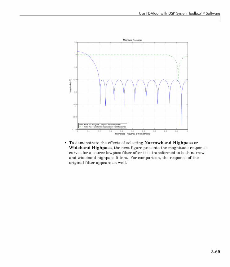
Use FDATool with DSP System Toolbox™ Software
0 0.1 0.2 0.3 0.4 0.5 0.6 0.7 0.8 0.9 1−120
−100
−80
−60
−40
−20
0
20
Normalized Frequency (×π rad/sample)
Mag
nitu
de (
dB)
Magnitude Response
Filter #1: Original Lowpass filter responseFilter #2: Transformed Lowpass Filter Response
• To demonstrate the effects of selecting Narrowband Highpass orWideband Highpass, the next figure presents the magnitude responsecurves for a source lowpass filter after it is transformed to both narrow-and wideband highpass filters. For comparison, the response of theoriginal filter appears as well.
3-69
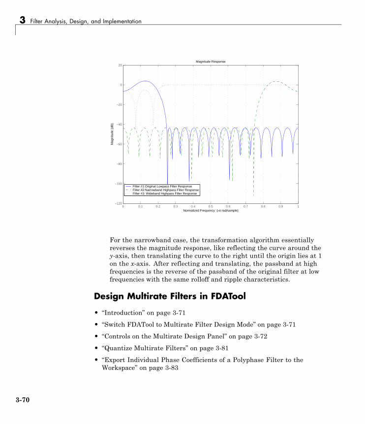
3 Filter Analysis, Design, and Implementation
0 0.1 0.2 0.3 0.4 0.5 0.6 0.7 0.8 0.9 1−120
−100
−80
−60
−40
−20
0
20
Normalized Frequency (×π rad/sample)
Mag
nitu
de (
dB)
Magnitude Response
Filter #1:Original Lowpass Filter ResponseFilter #2:Narrowband Highpass Filter ResponseFilter #3: Wideband Highpass Filter Response
For the narrowband case, the transformation algorithm essentiallyreverses the magnitude response, like reflecting the curve around they-axis, then translating the curve to the right until the origin lies at 1on the x-axis. After reflecting and translating, the passband at highfrequencies is the reverse of the passband of the original filter at lowfrequencies with the same rolloff and ripple characteristics.
Design Multirate Filters in FDATool
• “Introduction” on page 3-71
• “Switch FDATool to Multirate Filter Design Mode” on page 3-71
• “Controls on the Multirate Design Panel” on page 3-72
• “Quantize Multirate Filters” on page 3-81
• “Export Individual Phase Coefficients of a Polyphase Filter to theWorkspace” on page 3-83
3-70
Use FDATool with DSP System Toolbox™ Software
IntroductionNot only can you design multirate filters from the MATLAB command prompt,FDATool provides the same design capability in a graphical user interfacetool. By starting FDATool and switching to the multirate filter design modeyou have access to all of the multirate design capabilities in the toolbox —decimators, interpolators, and fractional rate changing filters, among others.
Switch FDATool to Multirate Filter Design ModeThe multirate filter design mode in FDATool lets you specify and design awide range of multirate filters, including decimators and interpolators.
With FDATool open, click Create a Multirate Filter, , on the side bar.You see FDATool switch to the design mode showing the multirate filterdesign options. Shown in the following figure is the default multirate designconfiguration that designs an interpolating filter with an interpolation factorof 2. The design uses the current FIR filter in FDATool.
3-71
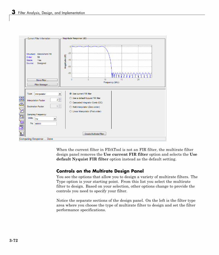
3 Filter Analysis, Design, and Implementation
When the current filter in FDATool is not an FIR filter, the multirate filterdesign panel removes the Use current FIR filter option and selects the Usedefault Nyquist FIR filter option instead as the default setting.
Controls on the Multirate Design PanelYou see the options that allow you to design a variety of multirate filters. TheType option is your starting point. From this list you select the multiratefilter to design. Based on your selection, other options change to provide thecontrols you need to specify your filter.
Notice the separate sections of the design panel. On the left is the filter typearea where you choose the type of multirate filter to design and set the filterperformance specifications.
3-72
Use FDATool with DSP System Toolbox™ Software
In the center section FDATool provides choices that let you pick the filterdesign method to use.
The rightmost section offers options that control filter configuration when youselect Cascaded-Integrator Comb (CIC) as the design method in the centersection. Both the Decimator type and Interpolator type filters let you usethe Cascaded-Integrator Comb (CIC) option to design multirate filters.
Here are all the options available when you switch to multirate filter designmode. Each option listed includes a brief description of what the option doeswhen you use it.
Select and Configure Your Filter
Option Description
Type Specifies the type of multirate filter to design.Choose from Decimator, Interpolator, orFractional-rate convertor.
• When you choose Decimator, set DecimationFactor to specify the decimation to apply.
• When you choose Interpolator, setInterpolation Factor to specify theinterpolation amount applied.
• When you choose Fractional-rate convertor,set both Interpolation Factor and DecimationFactor. FDATool uses both to determine thefractional rate change by dividing InterpolationFactor by Decimation Factor to determinethe fractional rate change in the signal. Youshould select values for interpolation anddecimation that are relatively prime. Whenyour interpolation factor and decimation factorare not relatively prime, FDATool reducesthe interpolation/decimation fractional rate tothe lowest common denominator and issuesa message in the status bar in FDATool. Forexample, if the interpolation factor is 6 and the
3-73

3 Filter Analysis, Design, and Implementation
Select and Configure Your Filter (Continued)
Option Description
decimation factor is 3, FDATool reduces 6/3 to2/1 when you design the rate changer. But if theinterpolation factor is 8 and the decimation factoris 3, FDATool designs the filter without change.
InterpolationFactor
Use the up-down control arrows to specify theamount of interpolation to apply to the signal.Factors range upwards from 2.
Decimation Factor Use the up-down control arrows to specify theamount of decimation to apply to the signal. Factorsrange upwards from 2.
SamplingFrequency
No settings here. Just Units and Fs below.
Units Specify whether Fs is specified in Hz, kHz, MHz, GHz,or Normalized (0 to 1) units.
Fs Set the full scale sampling frequency in thefrequency units you specified in Units. When youselect Normalized for Units, you do not enter avalue for Fs.
Design Your Filter
Option Description
Use current FIRfilter
Directs FDATool to use the current FIR filter todesign the multirate filter. If the current filter is anIIR form, you cannot select this option. You cannotdesign multirate filters with IIR structures.
Use a defaultNyquist Filter
Tells FDATool to use the default Nyquist designmethod when the current filter in FDATool is notan FIR filter.
CascadedIntegrator-Comb(CIC)
Design CIC filters using the options provided in theright-hand area of the multirate design panel.
3-74

Use FDATool with DSP System Toolbox™ Software
Design Your Filter (Continued)
Option Description
Hold Interpolator(Zero-order)
When you design an interpolator, you can specifyhow the filter sets interpolated values betweensignal values. When you select this option, theinterpolator applies the most recent signal value foreach interpolated value until it processes the nextsignal value. This is similar to sample-and-holdtechniques. Compare to the Linear Interpolatoroption.
Linear Interpolator(First-order)
When you design an interpolator, you can specifyhow the filter sets interpolated values betweensignal values. When you select this option, theinterpolator applies linear interpolation betweensignal value to set the interpolated value until itprocesses the next signal value. Compare to theLinear Interpolator option.
To see the difference between hold interpolation and linear interpolation, thefollowing figure presents a sine wave signal s1 in three forms:
• The top subplot in the figure presents signal s1 without interpolation.
• The middle subplot shows signal s1 interpolated by a linear interpolatorwith an interpolation factor of 5.
• The bottom subplot shows signal s1 interpolated by a hold interpolator withan interpolation factor of 5.
You see in the bottom figure the sample and hold nature of hold interpolation,and the first-order linear interpolation applied by the linear interpolator.
3-75
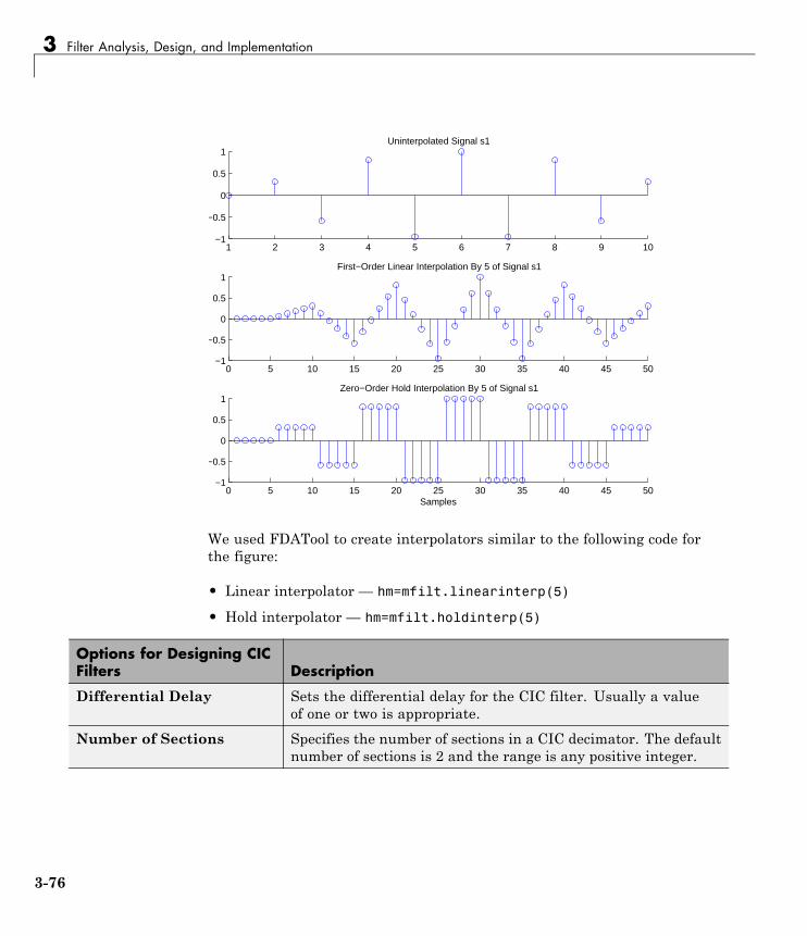
3 Filter Analysis, Design, and Implementation
1 2 3 4 5 6 7 8 9 10−1
−0.5
0
0.5
1Uninterpolated Signal s1
0 5 10 15 20 25 30 35 40 45 50−1
−0.5
0
0.5
1First−Order Linear Interpolation By 5 of Signal s1
0 5 10 15 20 25 30 35 40 45 50−1
−0.5
0
0.5
1
Samples
Zero−Order Hold Interpolation By 5 of Signal s1
We used FDATool to create interpolators similar to the following code forthe figure:
• Linear interpolator — hm=mfilt.linearinterp(5)
• Hold interpolator — hm=mfilt.holdinterp(5)
Options for Designing CICFilters Description
Differential Delay Sets the differential delay for the CIC filter. Usually a valueof one or two is appropriate.
Number of Sections Specifies the number of sections in a CIC decimator. The defaultnumber of sections is 2 and the range is any positive integer.
3-76
Use FDATool with DSP System Toolbox™ Software
Design a Fractional Rate Convertor. To introduce the process you use todesign a multirate filter in FDATool, this example uses the options to designa fractional rate convertor which uses 7/3 as the fractional rate. Begin thedesign by creating a default lowpass FIR filter in FDATool. You do not haveto begin with this FIR filter, but the default filter works fine.
1 Launch FDATool.
2 Select the settings for a minimum-order lowpass FIR filter, using theEquiripple design method.
3 When FDATool displays the magnitude response for the filter, click inthe side bar. FDATool switches to multirate filter design mode, showingthe multirate design panel.
4 To design a fractional rate filter, select Fractional-rate convertorfrom the Type list. The Interpolation Factor and Decimation Factoroptions become available.
5 In Interpolation Factor, use the up arrow to set the interpolation factorto 7.
6 Using the up arrow in Decimation Factor, set 3 as the decimation factor.
7 Select Use a default Nyquist FIR filter. You could design the rateconvertor with the current FIR filter as well.
8 Enter 24000 to set Fs.
9 Click Create Multirate Filter.
After designing the filter, FDATool returns with the specifications foryour new filter displayed in Current Filter Information, and showsthe magnitude response of the filter.
3-77
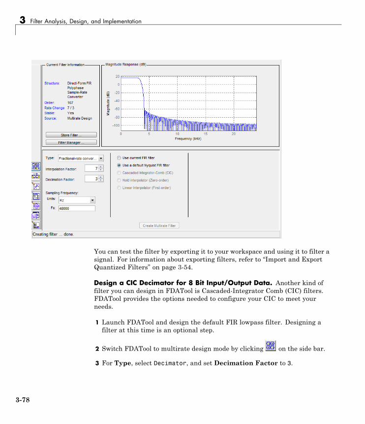
3 Filter Analysis, Design, and Implementation
You can test the filter by exporting it to your workspace and using it to filter asignal. For information about exporting filters, refer to “Import and ExportQuantized Filters” on page 3-54.
Design a CIC Decimator for 8 Bit Input/Output Data. Another kind offilter you can design in FDATool is Cascaded-Integrator Comb (CIC) filters.FDATool provides the options needed to configure your CIC to meet yourneeds.
1 Launch FDATool and design the default FIR lowpass filter. Designing afilter at this time is an optional step.
2 Switch FDATool to multirate design mode by clicking on the side bar.
3 For Type, select Decimator, and set Decimation Factor to 3.
3-78
Use FDATool with DSP System Toolbox™ Software
4 To design the decimator using a CIC implementation, selectCascaded-Integrator Comb (CIC). This enables the CIC-related optionson the right of the panel.
5 Set Differential Delay to 2. Generally, 1 or 2 are good values to use.
6 Enter 2 for the Number of Sections.
7 Click Create Multirate Filter.
FDATool designs the filter, shows the magnitude response in the analysisarea, and updates the current filter information to show that you designeda tenth-order cascaded-integrator comb decimator with two sections. Noticethe source is Multirate Design, indicating you used the multirate designmode in FDATool to make the filter. FDATool should look like this now.
3-79

3 Filter Analysis, Design, and Implementation
Designing other multirate filters follows the same pattern.
To design other multirate filters, do one of the following depending on thefilter to design:
• To design an interpolator, select one of these options.
- Use a default Nyquist FIR filter
- Cascaded-Integrator Comb (CIC)
- Hold Interpolator (Zero-order)
- Linear Interpolator (First-order)
3-80

Use FDATool with DSP System Toolbox™ Software
• To design a decimator, select from these options.
- Use a default Nyquist FIR filter
- Cascaded-Integrator Comb (CIC)
• To design a fractional-rate convertor, select Use a default Nyquist FIRfilter.
Quantize Multirate FiltersAfter you design a multirate filter in FDATool, the quantization featuresenable you to convert your floating-point multirate filter to fixed-pointarithmetic.
Note CIC filters are always fixed-point.
With your multirate filter as the current filter in FDATool, you can quantizeyour filter and use the quantization options to specify the fixed-pointarithmetic the filter uses.
Quantize and Configure Multirate Filters. Follow these steps to convertyour multirate filter to fixed-point arithmetic and set the fixed-point options.
1 Design or import your multirate filter and make sure it is the current filterin FDATool.
2 Click the Set Quantization Parameters button on the side bar.
3 From the Filter Arithmetic list on the Filter Arithmetic pane, selectFixed-point. If your filter is a CIC filter, the Fixed-point option isenabled by default and you do not set this option.
4 In the quantization panes, set the options for your filter. Set options forCoefficients, Input/Output, and Filter Internals.
5 Click Apply.
When you current filter is a CIC filter, the options on the Input/Output andFilter Internals panes change to provide specific features for CIC filters.
3-81
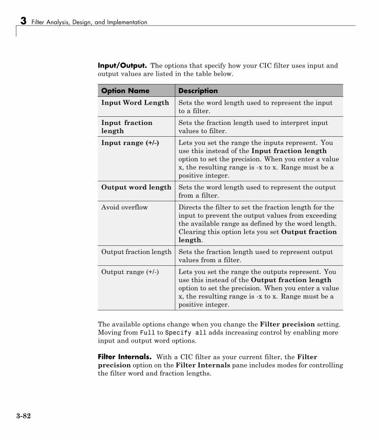
3 Filter Analysis, Design, and Implementation
Input/Output. The options that specify how your CIC filter uses input andoutput values are listed in the table below.
Option Name Description
Input Word Length Sets the word length used to represent the inputto a filter.
Input fractionlength
Sets the fraction length used to interpret inputvalues to filter.
Input range (+/-) Lets you set the range the inputs represent. Youuse this instead of the Input fraction lengthoption to set the precision. When you enter a valuex, the resulting range is -x to x. Range must be apositive integer.
Output word length Sets the word length used to represent the outputfrom a filter.
Avoid overflow Directs the filter to set the fraction length for theinput to prevent the output values from exceedingthe available range as defined by the word length.Clearing this option lets you set Output fractionlength.
Output fraction length Sets the fraction length used to represent outputvalues from a filter.
Output range (+/-) Lets you set the range the outputs represent. Youuse this instead of the Output fraction lengthoption to set the precision. When you enter a valuex, the resulting range is -x to x. Range must be apositive integer.
The available options change when you change the Filter precision setting.Moving from Full to Specify all adds increasing control by enabling moreinput and output word options.
Filter Internals. With a CIC filter as your current filter, the Filterprecision option on the Filter Internals pane includes modes for controllingthe filter word and fraction lengths.
3-82

Use FDATool with DSP System Toolbox™ Software
There are four usage modes for this (the same mode you select for theFilterInternals property in CIC filters at the MATLAB prompt).
• Full— All word and fraction lengths set to Bmax + 1, called Baccum by Harrisin [2]. Full Precision is the default setting.
• Minimum section word lengths — Set the section word lengths tominimum values that meet roundoff noise and output requirements asdefined by Hogenauer in [3].
• Specify word lengths — Enables the Section word length option foryou to enter word lengths for each section. Enter either a scalar to use thesame value for every section, or a vector of values, one for each section.
• Specify all— Enables the Section fraction length option in additionto Section word length. Now you can provide both the word and fractionlengths for each section, again using either a scalar or a vector of values.
Export Individual Phase Coefficients of a Polyphase Filter tothe WorkspaceAfter designing a polyphase filter in Filter Design Analysis Tool (FDATool),you can obtain the individual phase coefficients of the filter by:
1 Exporting the filter to an object in the MATLAB workspace.
2 Using the polyphase method to create a matrix of the filter’s coefficients.
Export the Polyphase Filter to an Object. To export a polyphase filter toan object in the MATLAB workspace, complete the following steps.
1 In FDATool, open the File menu and select Export.... This opens thedialog box for exporting the filter coefficients.
2 In the Export dialog box, for Export To, selectWorkspace.
3 For Export As, select Object.
4 (Optional) For Variable Names, enter the name of the Multirate Filterobject that will be created in the MATLAB workspace.
3-83

3 Filter Analysis, Design, and Implementation
5 Click the Export button. The multirate filter object, Hm in this example,appears in the MATLAB workspace.
Create a Matrix of Coefficients Using the polyphase Method. To createa matrix of the filter’s coefficients, enter p=polyphase(Hm) at the commandline. The polyphase method creates a matrix, p, of filter coefficients from thefilter object, Hm. Each row of p consists of the coefficients of an individual phasesubfilter. The first row contains to the coefficients of the first phase subfilter,the second row contains those of the second phase subfilter, and so on.
Realize Filters as Simulink Subsystem Blocks
• “Introduction” on page 3-84
• “About the Realize Model Panel in FDATool” on page 3-84
IntroductionAfter you design or import a filter in FDATool, the realize model featurelets you create a Simulink subsystem block that implements your filter. Thegenerated filter subsystem block uses either the Digital Filter block or thedelay, gain, and sum blocks in Simulink. If you do not have a Fixed-PointDesigner™ license, FDATool still realizes your model using blocks infixed-point mode from Simulink, but you cannot run any model that includesyour filter subsystem block in Simulink.
About the Realize Model Panel in FDAToolTo access to the Realize Model panel and the options for realizing yourquantized filter as a Simulink subsystem block, switch FDATool to realize
model mode by clicking on the sidebar.
The following panel shows the options for configuring how FDAToolimplements your filter as a Simulink block.
3-84

Use FDATool with DSP System Toolbox™ Software
For information on these parameters, see the descriptions on the FilterRealization Wizard block reference page.
Realize a Filter Using FDATool. After your quantized filter in FDAToolis performing the way you want, with your desired phase and magnituderesponse, and with the right coefficients and form, follow these steps to realizeyour filter as a subsystem that you can use in a Simulink model.
1 Click Realize Model on the sidebar to change FDATool to realize modelmode.
2 From the Destination list under Model, select either:
• Current model— to add the realized filter subsystem to your currentmodel
• New model— to open a new Simulink model window and add your filtersubsystem to the new window
3 Provide a name for your new filter subsystem in the Name field.
4 Decide whether to overwrite an existing block with this new one, and selector clear the Overwrite generated ‘Filter’ block check box.
5 Select the Build model using basic elements check box to implementyour filter as a subsystem block that consists of Sum, Gain, and Delayblocks.
3-85

3 Filter Analysis, Design, and Implementation
6 Select or clear the optimizations to apply.
• Optimize for zero gains — removes zero gain blocks from the modelrealization
• Optimize for unity gains — replaces unity gain blocks with directconnections to adjacent blocks
• Optimize for negative gains — replaces negative gain blocks by achange of sign at the nearest sum block
• Optimize delay chains— replaces cascaded delay blocks with a singledelay block that produces the equivalent gain
• Optimize for unity scale values — removes all scale valuemultiplications by 1 from the filter structure
7 Click Realize Model to realize your quantized filter as a subsystem blockaccording to the settings you selected.
If you double-click the filter block subsystem created by FDATool, you see thefilter implementation in Simulink model form. Depending on the options youchose when you realized your filter, and the filter you started with, you mightsee one or more sections, or different architectures based on the form of yourquantized filter. From this point on, the subsystem filter block acts like anyother block that you use in Simulink models.
Supported Filter Structures. FDATool lets you realize discrete-time andmultirate filters from the following forms:
Structure Description
firdecim Decimators based on FIR filters
firtdecim Decimators based on transposed FIRfilters
linearinterp Linear interpolators
firinterp Interpolators based on FIR filters
multirate polyphase Multirate filters
holdinterp Interpolators that use the holdinterpolation algorithm
3-86

Use FDATool with DSP System Toolbox™ Software
Structure Description
dfilt.allpass Discrete-time filters with allpassstructure
dfilt.cascadeallpass
dfilt.cascadewdfallpass
mfilt.iirdecim Decimators based on IIR filters
mfilt.iirwdfdecim
mfilt.iirinterp Interpolators based on IIR filters
mfilt.iirwdfinterp
dfilt.wdfallpass
3-87

3 Filter Analysis, Design, and Implementation
Digital Frequency Transformations
In this section...
“Details and Methodology” on page 3-88
“Frequency Transformations for Real Filters” on page 3-96
“Frequency Transformations for Complex Filters” on page 3-110
Details and Methodology
• “Overview of Transformations” on page 3-88
• “Select Features Subject to Transformation” on page 3-92
• “Mapping from Prototype Filter to Target Filter” on page 3-94
• “Summary of Frequency Transformations” on page 3-96
Overview of TransformationsConverting existing FIR or IIR filter designs to a modified IIR form is oftendone using allpass frequency transformations. Although the resulting designscan be considerably more expensive in terms of dimensionality than theprototype (original) filter, their ease of use in fixed or variable applications isa big advantage.
The general idea of the frequency transformation is to take an existingprototype filter and produce another filter from it that retains some of thecharacteristics of the prototype, in the frequency domain. Transformationfunctions achieve this by replacing each delaying element of the prototypefilter with an allpass filter carefully designed to have a prescribed phasecharacteristic for achieving the modifications requested by the designer.
The basic form of mapping commonly used is
H z H H zT o A( ) [ ( )]=
The HA(z) is an Nth-order allpass mapping filter given by
3-88

Digital Frequency Transformations
H z S
z
z
N zD zA
ii
i
N
iN i
i
NA
A( )
( )( )
= =
=
−
=
− +
=
∑
∑
0
0
0 1
where
Ho(z) — Transfer function of the prototype filter
HA(z) — Transfer function of the allpass mapping filter
HT(z) — Transfer function of the target filter
Let’s look at a simple example of the transformation given by
H z H zT o( ) ( )= −
The target filter has its poles and zeroes flipped across the origin of the realand imaginary axes. For the real filter prototype, it gives a mirror effectagainst 0.5, which means that lowpass Ho(z) gives rise to a real highpassHT(z). This is shown in the following figure for the prototype filter designed asa third-order halfband elliptic filter.
3-89

3 Filter Analysis, Design, and Implementation
0 0.2 0.4 0.6 0.8 1−60
−50
−40
−30
−20
−10
0Prototype filter
|H(ω
)| in
dB
Normalized Frequency (×π rad/sample)0 0.2 0.4 0.6 0.8 1
−60
−50
−40
−30
−20
−10
0Target filter
|H(ω
)| in
dB
Normalized Frequency (×π rad/sample)
Prototype filter Pole−Zero plot Target filter Pole−Zero plot
Example of a Simple Mirror Transformation
The choice of an allpass filter to provide the frequency mapping is necessaryto provide the frequency translation of the prototype filter frequency responseto the target filter by changing the frequency position of the features from theprototype filter without affecting the overall shape of the filter response.
The phase response of the mapping filter normalized to π can be interpretedas a translation function:
H wnew old( ) =
The graphical interpretation of the frequency transformation is shown in thefigure below. The complex multiband transformation takes a real lowpassfilter and converts it into a number of passbands around the unit circle.
3-90
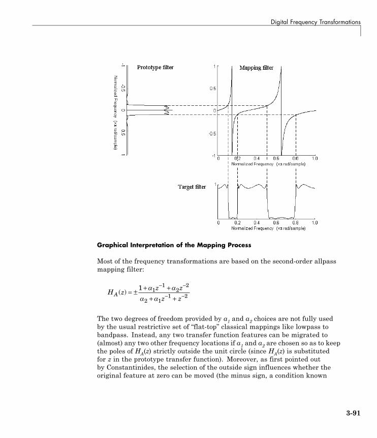
Digital Frequency Transformations
Graphical Interpretation of the Mapping Process
Most of the frequency transformations are based on the second-order allpassmapping filter:
H zz z
z zA( ) = ± + +
+ +
− −
− −1 1
12
2
2 11 2
The two degrees of freedom provided by α1 and α2 choices are not fully usedby the usual restrictive set of “flat-top” classical mappings like lowpass tobandpass. Instead, any two transfer function features can be migrated to(almost) any two other frequency locations if α1 and α2 are chosen so as to keepthe poles of HA(z) strictly outside the unit circle (since HA(z) is substitutedfor z in the prototype transfer function). Moreover, as first pointed outby Constantinides, the selection of the outside sign influences whether theoriginal feature at zero can be moved (the minus sign, a condition known
3-91

3 Filter Analysis, Design, and Implementation
as “DC mobility”) or whether the Nyquist frequency can be migrated (the“Nyquist mobility” case arising when the leading sign is positive).
All the transformations forming the package are explained in the nextsections of the tutorial. They are separated into those operating on realfilters and those generating or working with complex filters. The choice oftransformation ranges from standard Constantinides first and second-orderones [1][2] up to the real multiband filter by Mullis and Franchitti [3], andthe complex multiband filter and real/complex multipoint ones by Krukowski,Cain and Kale [4].
Select Features Subject to TransformationChoosing the appropriate frequency transformation for achieving the requiredeffect and the correct features of the prototype filter is very importantand needs careful consideration. It is not advisable to use a first-ordertransformation for controlling more than one feature. The mapping filterwill not give enough flexibility. It is also not good to use higher ordertransformation just to change the cutoff frequency of the lowpass filter. Theincrease of the filter order would be too big, without considering the additionalreplica of the prototype filter that may be created in undesired places.
Feature Selection for Real Lowpass to Bandpass Transformation
3-92

Digital Frequency Transformations
To illustrate the idea, the second-order real multipoint transformation wasapplied three times to the same elliptic halfband filter in order to make itinto a bandpass filter. In each of the three cases, two different features ofthe prototype filter were selected in order to obtain a bandpass filter withpassband ranging from 0.25 to 0.75. The position of the DC feature was notimportant, but it would be advantageous if it were in the middle betweenthe edges of the passband in the target filter. In the first case the selectedfeatures were the left and the right band edges of the lowpass filter passband,in the second case they were the left band edge and the DC, in the third casethey were DC and the right band edge.
0 0.1 0.2 0.3 0.4 0.5 0.6 0.7 0.8 0.9 1−60
−50
−40
−30
−20
−10
0
Left & right band−edges (solid)
Left band−edge and DC (dashed)
DC and right band−edges (dotted)
Magniture responses |H(ω)| in dB
Normalized Frequency (×π rad/sample)
Result of Choosing Different Features
The results of all three approaches are completely different. For each of themonly the selected features were positioned precisely where they were required.In the first case the DC is moved toward the left passband edge just like allthe other features close to the left edge being squeezed there. In the secondcase the right passband edge was pushed way out of the expected target asthe precise position of DC was required. In the third case the left passbandedge was pulled toward the DC in order to position it at the correct frequency.
3-93

3 Filter Analysis, Design, and Implementation
The conclusion is that if only the DC can be anywhere in the passband, theedges of the passband should have been selected for the transformation. Formost of the cases requiring the positioning of passbands and stopbands,designers should always choose the position of the edges of the prototypefilter in order to make sure that they get the edges of the target filter in thecorrect places. Frequency responses for the three cases considered are shownin the figure. The prototype filter was a third-order elliptic lowpass filterwith cutoff frequency at 0.5.
The MATLAB code used to generate the figure is given here.
The prototype filter is a halfband elliptic, real, third-order lowpass filter:
[b, a] = ellip(3, 0.1, 30, 0.409);
In the example the requirements are set to create a real bandpass filterwith passband edges at 0.1 and 0.3 out of the real lowpass filter having thecutoff frequency at 0.5. This is attempted in three different ways. In the firstapproach both edges of the passband are selected, in the second approach theleft edge of the passband and the DC are chosen, while in the third approachthe DC and the right edge of the passband are taken:
[num1,den1] = iirlp2xn(b, a, [-0.5, 0.5], [0.1, 0.3]);[num2,den2] = iirlp2xn(b, a, [-0.5, 0.0], [0.1, 0.2]);[num3,den3] = iirlp2xn(b, a, [ 0.0, 0.5], [0.2, 0.3]);
Mapping from Prototype Filter to Target FilterIn general the frequency mapping converts the prototype filter, Ho(z), to thetarget filter, HT(z), using the NAth-order allpass filter, HA(z). The generalform of the allpass mapping filter is given in “Overview of Transformations”on page 3-88. The frequency mapping is a mathematical operation thatreplaces each delayer of the prototype filter with an allpass filter. Thereare two ways of performing such mapping. The choice of the approach isdependent on how prototype and target filters are represented.
When the Nth-order prototype filter is given with pole-zero form
3-94
Digital Frequency Transformations
H z
z z
z po
ii
N
ii
N( )
( )
( )
=−
−
=
=
∑
∑1
1
the mapping will replace each pole, pi, and each zero, zi, with a number ofpoles and zeros equal to the order of the allpass mapping filter:
H z
S z z z
S zo
i
N
kk
i kN k
k
N
k
N
i
N
kk
( ) =
− ⋅⎛
⎝⎜⎜
⎞
⎠⎟⎟
=
−
=
−
=
−
=
∑ ∑∑
∑1 0
1
0
1
1
−− ⋅⎛
⎝⎜⎜
⎞
⎠⎟⎟
−
=
−
=
−
∑∑ p zi kN k
k
N
k
N
0
1
0
1
The root finding needs to be used on the bracketed expressions in order to findthe poles and zeros of the target filter.
When the prototype filter is described in the numerator-denominator form:
H zz z
z zT
N NN
N NN z H zA
( )( )
=+ + ++ + +
−
−=
0 1
1
0 11
Then the mapping process will require a number of convolutions in order tocalculate the numerator and denominator of the target filter:
H zN z N z D z D z
N z N zT
AN
AN
A N AN
AN
AN
( )( ) ( ) ( ) ( )
( ) ( )=
+ + ++
−
1 2
1
1 2
−− + +1 D z D zA N A
N( ) ( )
For each coefficient αi and βi of the prototype filter the NAth-order polynomialsmust be convolved N times. Such approach may cause rounding errors forlarge prototype filters and/or high order mapping filters. In such a case theuser should consider the alternative of doing the mapping using via polesand zeros.
3-95

3 Filter Analysis, Design, and Implementation
Summary of Frequency Transformations
Advantages.
• Most frequency transformations are described by closed-form solutions orcan be calculated from the set of linear equations.
• They give predictable and familiar results.
• Ripple heights from the prototype filter are preserved in the target filter.
• They are architecturally appealing for variable and adaptive filters.
Disadvantages.
• There are cases when using optimization methods to design the requiredfilter gives better results.
• High-order transformations increase the dimensionality of the target filter,which may give expensive final results.
• Starting from fresh designs helps avoid locked-in compromises.
Frequency Transformations for Real Filters
• “Overview” on page 3-96
• “Real Frequency Shift” on page 3-97
• “Real Lowpass to Real Lowpass” on page 3-98
• “Real Lowpass to Real Highpass” on page 3-100
• “Real Lowpass to Real Bandpass” on page 3-102
• “Real Lowpass to Real Bandstop” on page 3-104
• “Real Lowpass to Real Multiband” on page 3-106
• “Real Lowpass to Real Multipoint” on page 3-108
OverviewThis section discusses real frequency transformations that take the reallowpass prototype filter and convert it into a different real target filter. Thetarget filter has its frequency response modified in respect to the frequency
3-96
Digital Frequency Transformations
response of the prototype filter according to the characteristic of the appliedfrequency transformation.
Real Frequency ShiftReal frequency shift transformation uses a second-order allpass mappingfilter. It performs an exact mapping of one selected feature of the frequencyresponse into its new location, additionally moving both the Nyquist and DCfeatures. This effectively moves the whole response of the lowpass filter bythe distance specified by the selection of the feature from the prototype filterand the target filter. As a real transformation, it works in a similar wayfor positive and negative frequencies.
H z zz
zA( ) = ⋅ −
−−
−
−1
1
11
with α given by
=
−− <
cos ( )
coscos ( )
sin (
22
22
2 1
2
old new
old
old new
o
for
lld new
old
otherwise−
⎧
⎨
⎪⎪⎪⎪
⎩
⎪⎪⎪⎪
2
2
)
sin
where
ωold— Frequency location of the selected feature in the prototype filter
ωnew— Position of the feature originally at ωold in the target filter
The following example shows how this transformation can be used to movethe response of the prototype lowpass filter in either direction. Please notethat because the target filter must also be real, the response of the targetfilter will inherently be disturbed at frequencies close to Nyquist and close toDC. Here is the MATLAB code for generating the example in the figure.
3-97
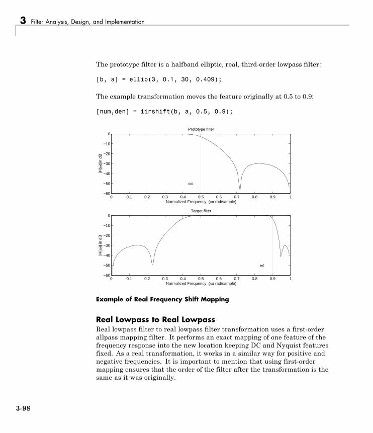
3 Filter Analysis, Design, and Implementation
The prototype filter is a halfband elliptic, real, third-order lowpass filter:
[b, a] = ellip(3, 0.1, 30, 0.409);
The example transformation moves the feature originally at 0.5 to 0.9:
[num,den] = iirshift(b, a, 0.5, 0.9);
0 0.1 0.2 0.3 0.4 0.5 0.6 0.7 0.8 0.9 1−60
−50
−40
−30
−20
−10
0Prototype filter
|H(ω
)|in
dB
Normalized Frequency (×π rad/sample)
ωo
0 0.1 0.2 0.3 0.4 0.5 0.6 0.7 0.8 0.9 1−60
−50
−40
−30
−20
−10
0Target filter
|H(ω
)| in
dB
Normalized Frequency (×π rad/sample)
ωt
Example of Real Frequency Shift Mapping
Real Lowpass to Real LowpassReal lowpass filter to real lowpass filter transformation uses a first-orderallpass mapping filter. It performs an exact mapping of one feature of thefrequency response into the new location keeping DC and Nyquist featuresfixed. As a real transformation, it works in a similar way for positive andnegative frequencies. It is important to mention that using first-ordermapping ensures that the order of the filter after the transformation is thesame as it was originally.
3-98
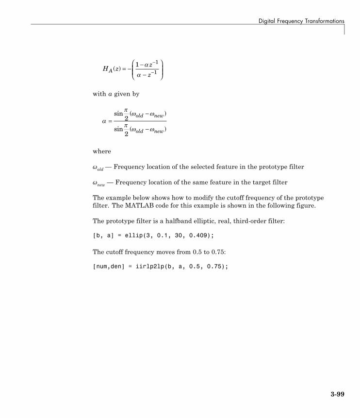
Digital Frequency Transformations
H zz
zA( ) = − −
−
⎛
⎝⎜⎜
⎞
⎠⎟⎟
−
−1 1
1
with α given by
=
−
−
sin ( )
sin ( )
2
2
old new
old new
where
ωold— Frequency location of the selected feature in the prototype filter
ωnew— Frequency location of the same feature in the target filter
The example below shows how to modify the cutoff frequency of the prototypefilter. The MATLAB code for this example is shown in the following figure.
The prototype filter is a halfband elliptic, real, third-order filter:
[b, a] = ellip(3, 0.1, 30, 0.409);
The cutoff frequency moves from 0.5 to 0.75:
[num,den] = iirlp2lp(b, a, 0.5, 0.75);
3-99
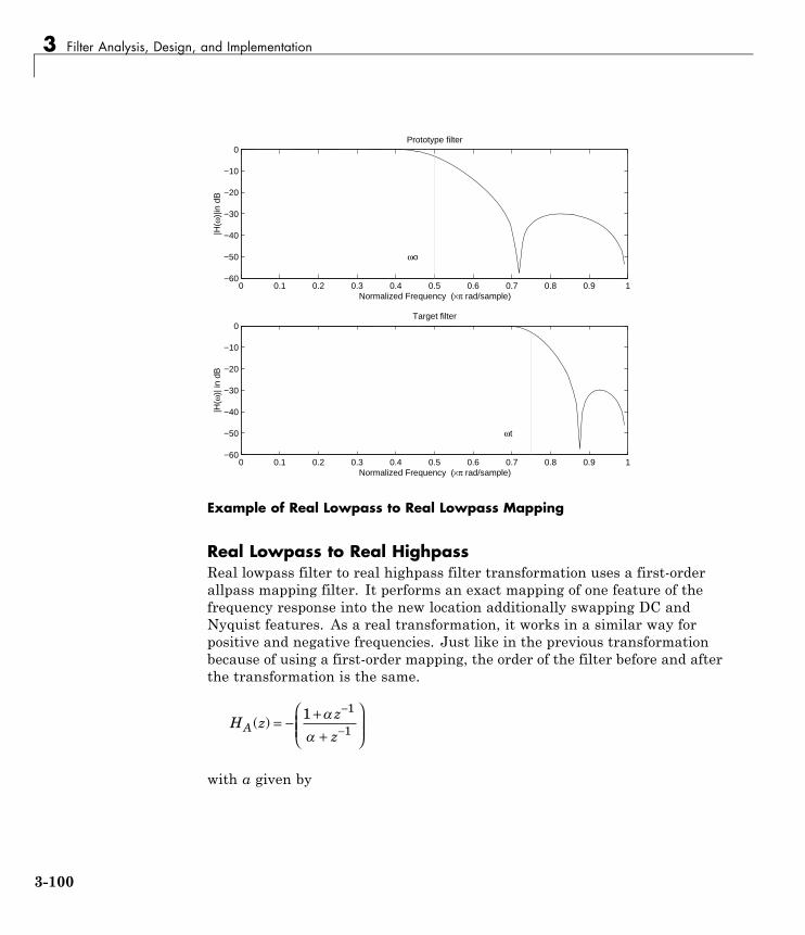
3 Filter Analysis, Design, and Implementation
0 0.1 0.2 0.3 0.4 0.5 0.6 0.7 0.8 0.9 1−60
−50
−40
−30
−20
−10
0Prototype filter
|H(ω
)|in
dB
Normalized Frequency (×π rad/sample)
ωo
0 0.1 0.2 0.3 0.4 0.5 0.6 0.7 0.8 0.9 1−60
−50
−40
−30
−20
−10
0Target filter
|H(ω
)| in
dB
Normalized Frequency (×π rad/sample)
ωt
Example of Real Lowpass to Real Lowpass Mapping
Real Lowpass to Real HighpassReal lowpass filter to real highpass filter transformation uses a first-orderallpass mapping filter. It performs an exact mapping of one feature of thefrequency response into the new location additionally swapping DC andNyquist features. As a real transformation, it works in a similar way forpositive and negative frequencies. Just like in the previous transformationbecause of using a first-order mapping, the order of the filter before and afterthe transformation is the same.
H zz
zA( ) = − +
+
⎛
⎝⎜⎜
⎞
⎠⎟⎟
−
−1 1
1
with α given by
3-100

Digital Frequency Transformations
= −
+
−
⎛
⎝
⎜⎜⎜
⎞
⎠
⎟⎟⎟
cos ( )
cos ( )
2
2
old new
old new
where
ωold— Frequency location of the selected feature in the prototype filter
ωnew— Frequency location of the same feature in the target filter
The example below shows how to convert the lowpass filter into a highpassfilter with arbitrarily chosen cutoff frequency. In the MATLAB code below,the lowpass filter is converted into a highpass with cutoff frequency shiftedfrom 0.5 to 0.75. Results are shown in the figure.
The prototype filter is a halfband elliptic, real, third-order filter:
[b, a] = ellip(3, 0.1, 30, 0.409);
The example moves the cutoff frequency from 0.5 to 0.75:
[num,den] = iirlp2hp(b, a, 0.5, 0.75);
3-101
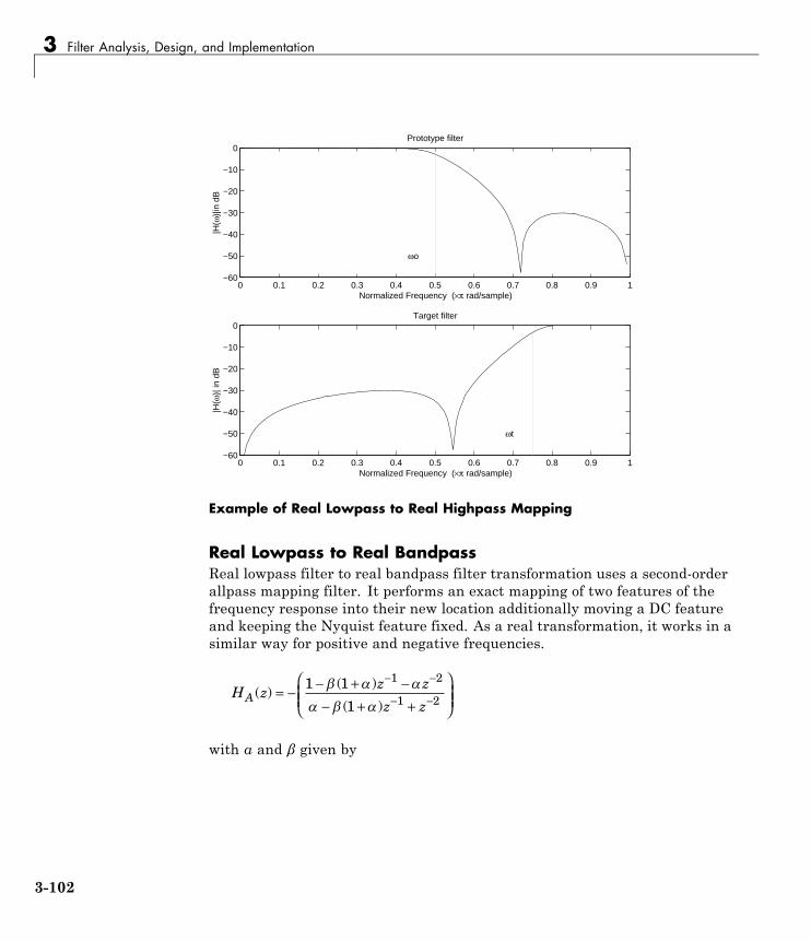
3 Filter Analysis, Design, and Implementation
0 0.1 0.2 0.3 0.4 0.5 0.6 0.7 0.8 0.9 1−60
−50
−40
−30
−20
−10
0Prototype filter
|H(ω
)|in
dB
Normalized Frequency (×π rad/sample)
ωo
0 0.1 0.2 0.3 0.4 0.5 0.6 0.7 0.8 0.9 1−60
−50
−40
−30
−20
−10
0Target filter
|H(ω
)| in
dB
Normalized Frequency (×π rad/sample)
ωt
Example of Real Lowpass to Real Highpass Mapping
Real Lowpass to Real BandpassReal lowpass filter to real bandpass filter transformation uses a second-orderallpass mapping filter. It performs an exact mapping of two features of thefrequency response into their new location additionally moving a DC featureand keeping the Nyquist feature fixed. As a real transformation, it works in asimilar way for positive and negative frequencies.
H zz z
z zA( )
( )
( )= − − + −
− + +
⎛
⎝⎜⎜
⎞
⎠⎟⎟
− −
− −1 1
1
1 2
1 2
with α and β given by
3-102
Digital Frequency Transformations
=
− +
+ −
sin ( )
sin ( )
, ,
, ,
42
42
2 1
2 1
old new new
old new new
= +cos ( ), ,2 1 2new new
where
ωold— Frequency location of the selected feature in the prototype filter
ωnew,1— Position of the feature originally at (-ωold) in the target filter
ωnew,2— Position of the feature originally at (+ωold) in the target filter
The example below shows how to move the response of the prototype lowpassfilter in either direction. Please note that because the target filter mustalso be real, the response of the target filter will inherently be disturbed atfrequencies close to Nyquist and close to DC. Here is the MATLAB code forgenerating the example in the figure.
The prototype filter is a halfband elliptic, real, third-order lowpass filter:
[b, a] = ellip(3, 0.1, 30, 0.409);
The example transformation creates the passband between 0.5 and 0.75:
[num,den] = iirlp2bp(b, a, 0.5, [0.5, 0.75]);
3-103

3 Filter Analysis, Design, and Implementation
0 0.1 0.2 0.3 0.4 0.5 0.6 0.7 0.8 0.9 1−60
−50
−40
−30
−20
−10
0Prototype filter
|H(ω
)|in
dB
Normalized Frequency (×π rad/sample)
ωo
0 0.1 0.2 0.3 0.4 0.5 0.6 0.7 0.8 0.9 1−60
−50
−40
−30
−20
−10
0Target filter
|H(ω
)| in
dB
Normalized Frequency (×π rad/sample)
ωt1 ωt2
Example of Real Lowpass to Real Bandpass Mapping
Real Lowpass to Real BandstopReal lowpass filter to real bandstop filter transformation uses a second-orderallpass mapping filter. It performs an exact mapping of two features ofthe frequency response into their new location additionally moving aNyquist feature and keeping the DC feature fixed. This effectively createsa stopband between the selected frequency locations in the target filter. Asa real transformation, it works in a similar way for positive and negativefrequencies.
H zz z
z zA( )
( )
( )= − + +
− + +
− −
− −1 1
1
1 2
1 2
with α and β given by
3-104
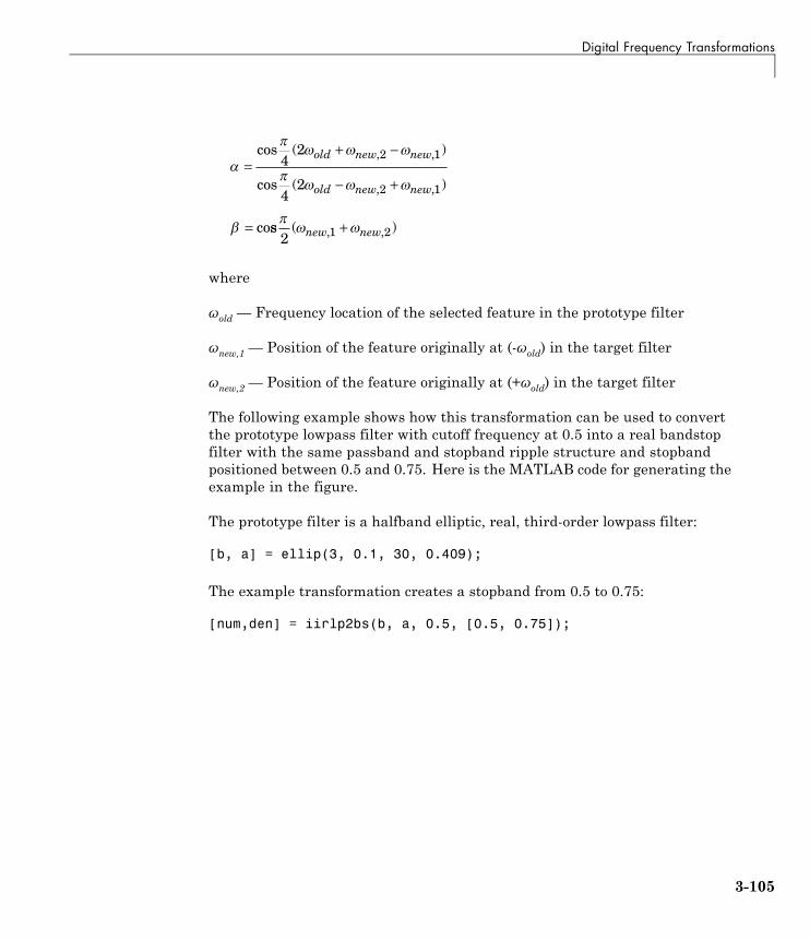
Digital Frequency Transformations
=+ −
− +
=
cos ( )
cos ( )
co
, ,
, ,
42
42
2 1
2 1
old new new
old new new
ss ( ), ,
2 1 2new new+
where
ωold— Frequency location of the selected feature in the prototype filter
ωnew,1— Position of the feature originally at (-ωold) in the target filter
ωnew,2— Position of the feature originally at (+ωold) in the target filter
The following example shows how this transformation can be used to convertthe prototype lowpass filter with cutoff frequency at 0.5 into a real bandstopfilter with the same passband and stopband ripple structure and stopbandpositioned between 0.5 and 0.75. Here is the MATLAB code for generating theexample in the figure.
The prototype filter is a halfband elliptic, real, third-order lowpass filter:
[b, a] = ellip(3, 0.1, 30, 0.409);
The example transformation creates a stopband from 0.5 to 0.75:
[num,den] = iirlp2bs(b, a, 0.5, [0.5, 0.75]);
3-105

3 Filter Analysis, Design, and Implementation
0 0.1 0.2 0.3 0.4 0.5 0.6 0.7 0.8 0.9 1−60
−50
−40
−30
−20
−10
0Prototype filter
|H(ω
)|in
dB
Normalized Frequency (×π rad/sample)
ωo
0 0.1 0.2 0.3 0.4 0.5 0.6 0.7 0.8 0.9 1−60
−50
−40
−30
−20
−10
0Target filter
|H(ω
)| in
dB
Normalized Frequency (×π rad/sample)
ωt1 ωt2
Example of Real Lowpass to Real Bandstop Mapping
Real Lowpass to Real MultibandThis high-order transformation performs an exact mapping of one selectedfeature of the prototype filter frequency response into a number of newlocations in the target filter. Its most common use is to convert a real lowpasswith predefined passband and stopband ripples into a real multiband filterwith N arbitrary band edges, where N is the order of the allpass mappingfilter.
H z S
z
zA
ii
i
N
iN i
i
N( ) =
=
−
=
− +
=
∑
∑
0
0
0 1
3-106
Digital Frequency Transformations
The coefficients α are given by
0 1 1
21
22 1
= =
= −+ −
− + −
k N
SN
N kk
newk
old
new
, ,
sin ( ( ) )
sin (( ) (
)) )kold
⎧
⎨
⎪⎪
⎩
⎪⎪
where
ωold,k— Frequency location of the first feature in the prototype filter
ωnew,k— Position of the feature originally at ωold,k in the target filter
The mobility factor, S, specifies the mobility or either DC or Nyquist feature:
SNyquist
DC=
−⎧⎨⎩
11
The example below shows how this transformation can be used to convert theprototype lowpass filter with cutoff frequency at 0.5 into a filter having anumber of bands positioned at arbitrary edge frequencies 1/5, 2/5, 3/5 and 4/5.Parameter S was such that there is a passband at DC. Here is the MATLABcode for generating the figure.
The prototype filter is a halfband elliptic, real, third-order lowpass filter:
[b, a] = ellip(3, 0.1, 30, 0.409);
The example transformation creates three stopbands, from DC to 0.2, from0.4 to 0.6 and from 0.8 to Nyquist:
[num,den] = iirlp2mb(b, a, 0.5, [0.2, 0.4, 0.6, 0.8], `pass');
3-107
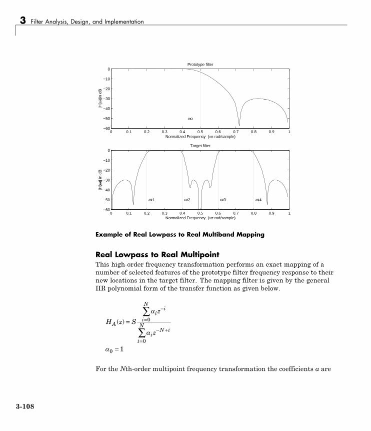
3 Filter Analysis, Design, and Implementation
0 0.1 0.2 0.3 0.4 0.5 0.6 0.7 0.8 0.9 1−60
−50
−40
−30
−20
−10
0Prototype filter
|H(ω
)|in
dB
Normalized Frequency (×π rad/sample)
ωo
0 0.1 0.2 0.3 0.4 0.5 0.6 0.7 0.8 0.9 1−60
−50
−40
−30
−20
−10
0Target filter
|H(ω
)| in
dB
Normalized Frequency (×π rad/sample)
ωt1 ωt2 ωt3 ωt4
Example of Real Lowpass to Real Multiband Mapping
Real Lowpass to Real MultipointThis high-order frequency transformation performs an exact mapping of anumber of selected features of the prototype filter frequency response to theirnew locations in the target filter. The mapping filter is given by the generalIIR polynomial form of the transfer function as given below.
H z S
z
zA
ii
i
N
iN i
i
N( ) =
=
−
=
− +
=
∑
∑
0
0
0 1
For the Nth-order multipoint frequency transformation the coefficients α are
3-108
Digital Frequency Transformations
N i old k new ki
new kN i
old k new ki
N
old k
z z S z z S z
z
−−
=⋅ − ⋅ = − − ⋅∑ , , , , ,
,
1
==
=
=
⎧
⎨
⎪⎪⎪⎪
⎩
⎪⎪⎪⎪
e
z e
k N
j
new kj
old k
new k
,
,,
, ,1
where
ωold,k— Frequency location of the first feature in the prototype filter
ωnew,k— Position of the feature originally at ωold,k in the target filter
The mobility factor, S, specifies the mobility of either DC or Nyquist feature:
SNyquist
DC=
−⎧⎨⎩
11
The example below shows how this transformation can be used to movefeatures of the prototype lowpass filter originally at -0.5 and 0.5 to their newlocations at 0.5 and 0.75, effectively changing a position of the filter passband.Here is the MATLAB code for generating the figure.
The prototype filter is a halfband elliptic, real, third-order lowpass filter:
[b, a] = ellip(3, 0.1, 30, 0.409);
The example transformation creates a passband from 0.5 to 0.75:
[num,den] = iirlp2xn(b, a, [-0.5, 0.5], [0.5, 0.75], `pass');
3-109

3 Filter Analysis, Design, and Implementation
0 0.1 0.2 0.3 0.4 0.5 0.6 0.7 0.8 0.9 1−60
−50
−40
−30
−20
−10
0Prototype filter
|H(ω
)|in
dB
Normalized Frequency (×π rad/sample)
ωo2
0 0.1 0.2 0.3 0.4 0.5 0.6 0.7 0.8 0.9 1−60
−50
−40
−30
−20
−10
0Target filter
|H(ω
)| in
dB
Normalized Frequency (×π rad/sample)
ωt1 ωt2
Example of Real Lowpass to Real Multipoint Mapping
Frequency Transformations for Complex Filters
• “Overview” on page 3-110
• “Complex Frequency Shift” on page 3-111
• “Real Lowpass to Complex Bandpass” on page 3-112
• “Real Lowpass to Complex Bandstop” on page 3-114
• “Real Lowpass to Complex Multiband” on page 3-116
• “Real Lowpass to Complex Multipoint” on page 3-118
• “Complex Bandpass to Complex Bandpass” on page 3-120
OverviewThis section discusses complex frequency transformation that take thecomplex prototype filter and convert it into a different complex target
3-110
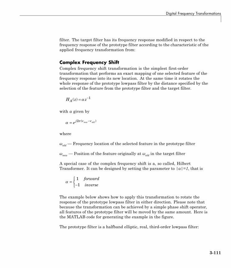
Digital Frequency Transformations
filter. The target filter has its frequency response modified in respect to thefrequency response of the prototype filter according to the characteristic of theapplied frequency transformation from:
Complex Frequency ShiftComplex frequency shift transformation is the simplest first-ordertransformation that performs an exact mapping of one selected feature of thefrequency response into its new location. At the same time it rotates thewhole response of the prototype lowpass filter by the distance specified by theselection of the feature from the prototype filter and the target filter.
H z zA( ) = − 1
with α given by
= −e j new old2 ( )
where
ωold— Frequency location of the selected feature in the prototype filter
ωnew— Position of the feature originally at ωold in the target filter
A special case of the complex frequency shift is a, so called, HilbertTransformer. It can be designed by setting the parameter to |α|=1, that is
=−
⎧⎨⎩
11
forwardinverse
The example below shows how to apply this transformation to rotate theresponse of the prototype lowpass filter in either direction. Please note thatbecause the transformation can be achieved by a simple phase shift operator,all features of the prototype filter will be moved by the same amount. Here isthe MATLAB code for generating the example in the figure.
The prototype filter is a halfband elliptic, real, third-order lowpass filter:
3-111

3 Filter Analysis, Design, and Implementation
[b, a] = ellip(3, 0.1, 30, 0.409);
The example transformation moves the feature originally at 0.5 to 0.3:
[num,den] = iirshiftc(b, a, 0.5, 0.3);
−1 −0.8 −0.6 −0.4 −0.2 0 0.2 0.4 0.6 0.8 1−60
−50
−40
−30
−20
−10
0Prototype filter
|H(ω
)|in
dB
Normalized Frequency (×π rad/sample)
ωo
−1 −0.8 −0.6 −0.4 −0.2 0 0.2 0.4 0.6 0.8 1−60
−50
−40
−30
−20
−10
0Target filter
|H(ω
)| in
dB
Normalized Frequency (×π rad/sample)
ωt
Example of Complex Frequency Shift Mapping
Real Lowpass to Complex BandpassThis first-order transformation performs an exact mapping of one selectedfeature of the prototype filter frequency response into two new locations inthe target filter creating a passband between them. Both Nyquist and DCfeatures can be moved with the rest of the frequency response.
H zz
zA( ) = −
−
−
−
1
1
with α and β are given by
3-112
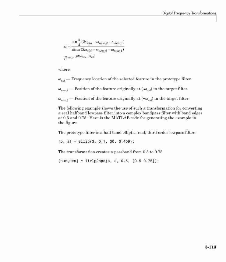
Digital Frequency Transformations
=− +
+ −
= −
sin ( )
sin ( )
, ,
, ,
42
2
2 1
2 1
old new new
old new new
je ( )new old−
where
ωold— Frequency location of the selected feature in the prototype filter
ωnew,1— Position of the feature originally at (-ωold) in the target filter
ωnew,2— Position of the feature originally at (+ωold) in the target filter
The following example shows the use of such a transformation for convertinga real halfband lowpass filter into a complex bandpass filter with band edgesat 0.5 and 0.75. Here is the MATLAB code for generating the example inthe figure.
The prototype filter is a half band elliptic, real, third-order lowpass filter:
[b, a] = ellip(3, 0.1, 30, 0.409);
The transformation creates a passband from 0.5 to 0.75:
[num,den] = iirlp2bpc(b, a, 0.5, [0.5 0.75]);
3-113

3 Filter Analysis, Design, and Implementation
−1 −0.8 −0.6 −0.4 −0.2 0 0.2 0.4 0.6 0.8 1−60
−50
−40
−30
−20
−10
0Prototype filter
|H(ω
)|in
dB
Normalized Frequency (×π rad/sample)
ωo
−1 −0.8 −0.6 −0.4 −0.2 0 0.2 0.4 0.6 0.8 1−60
−50
−40
−30
−20
−10
0Target filter
|H(ω
)| in
dB
Normalized Frequency (×π rad/sample)
ωt1
ωt2
Example of Real Lowpass to Complex Bandpass Mapping
Real Lowpass to Complex BandstopThis first-order transformation performs an exact mapping of one selectedfeature of the prototype filter frequency response into two new locations inthe target filter creating a stopband between them. Both Nyquist and DCfeatures can be moved with the rest of the frequency response.
H zz
zA( ) = −
−
−
−
1
1
with α and β are given by
=+ −− +
= −
cos ( )
cos ( ), ,
, ,
2
22 1
2 1
old new new
old new new
je (( ) new old−
3-114

Digital Frequency Transformations
where
ωold— Frequency location of the selected feature in the prototype filter
ωnew,1— Position of the feature originally at (-ωold) in the target filter
ωnew,2— Position of the feature originally at (+ωold) in the target filter
The example below shows the use of such a transformation for converting areal halfband lowpass filter into a complex bandstop filter with band edgesat 0.5 and 0.75. Here is the MATLAB code for generating the example inthe figure.
The prototype filter is a halfband elliptic, real, third-order lowpass filter:
[b, a] = ellip(3, 0.1, 30, 0.409);
The transformation creates a stopband from 0.5 to 0.75:
[num,den] = iirlp2bsc(b, a, 0.5, [0.5 0.75]);
3-115

3 Filter Analysis, Design, and Implementation
−1 −0.8 −0.6 −0.4 −0.2 0 0.2 0.4 0.6 0.8 1−60
−50
−40
−30
−20
−10
0Prototype filter
|H(ω
)|in
dB
Normalized Frequency (×π rad/sample)
ωo
−1 −0.8 −0.6 −0.4 −0.2 0 0.2 0.4 0.6 0.8 1−60
−50
−40
−30
−20
−10
0Target filter
|H(ω
)| in
dB
Normalized Frequency (×π rad/sample)
ωt1 ωt2
Example of Real Lowpass to Complex Bandstop Mapping
Real Lowpass to Complex MultibandThis high-order transformation performs an exact mapping of one selectedfeature of the prototype filter frequency response into a number of newlocations in the target filter. Its most common use is to convert a real lowpasswith predefined passband and stopband ripples into a multiband filterwith arbitrary band edges. The order of the mapping filter must be even,which corresponds to an even number of band edges in the target filter. TheNth-order complex allpass mapping filter is given by the following generaltransfer function form:
3-116
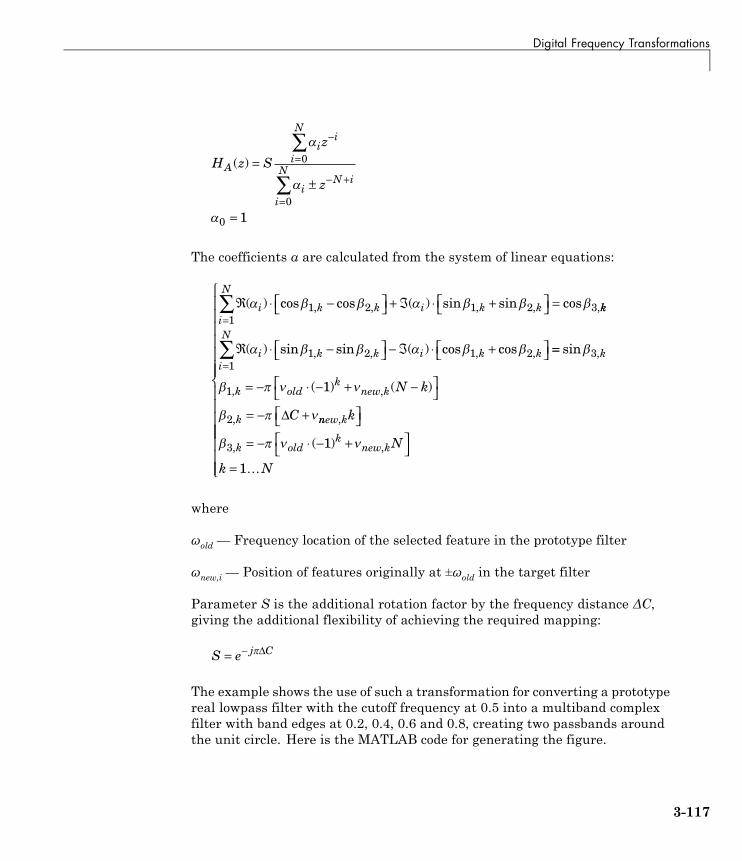
Digital Frequency Transformations
H z S
z
zA
ii
i
N
iN i
i
N( ) =
±
=
−
=
− +
=
∑
∑
0
0
0 1
The coefficients α are calculated from the system of linear equations:
ℜ ⋅ −⎡⎣ ⎤⎦ + ℑ ⋅ +⎡⎣ ⎤⎦ =( ) cos cos ( ) sin sin cos, , , , , i k k i k k1 2 1 2 3 kki
N
i k k i k k
=∑
ℜ ⋅ −⎡⎣ ⎤⎦ − ℑ ⋅ +⎡⎣ ⎤⎦
1
1 2 1 2( ) sin sin ( ) cos cos, , , , ==
= − ⋅ − + −⎡⎣
⎤⎦
= − +
=∑ sin
( ) ( )
,
, ,
,
31
1
2
1
ki
N
k oldk
new k
k
N k
CΔ nnew k
k oldk
new k
k
N
k N
,
, ,( )
⎡⎣ ⎤⎦
= − ⋅ − +⎡⎣
⎤⎦
=
⎧
⎨
⎪⎪⎪⎪⎪⎪⎪
⎩
⎪⎪⎪
3 1
1
⎪⎪⎪⎪⎪
where
ωold— Frequency location of the selected feature in the prototype filter
ωnew,i— Position of features originally at ±ωold in the target filter
Parameter S is the additional rotation factor by the frequency distance ΔC,giving the additional flexibility of achieving the required mapping:
S e j C= − Δ
The example shows the use of such a transformation for converting a prototypereal lowpass filter with the cutoff frequency at 0.5 into a multiband complexfilter with band edges at 0.2, 0.4, 0.6 and 0.8, creating two passbands aroundthe unit circle. Here is the MATLAB code for generating the figure.
3-117

3 Filter Analysis, Design, and Implementation
−1 −0.8 −0.6 −0.4 −0.2 0 0.2 0.4 0.6 0.8 1−60
−50
−40
−30
−20
−10
0Prototype filter
|H(ω
)|in
dB
Normalized Frequency (×π rad/sample)
ωo
−1 −0.8 −0.6 −0.4 −0.2 0 0.2 0.4 0.6 0.8 1−60
−50
−40
−30
−20
−10
0Target filter
|H(ω
)| in
dB
Normalized Frequency (×π rad/sample)
ωt1 ωt2 ωt3 ωt4
Example of Real Lowpass to Complex Multiband Mapping
The prototype filter is a halfband elliptic, real, third-order lowpass filter:
[b, a] = ellip(3, 0.1, 30, 0.409);
The example transformation creates two complex passbands:
[num,den] = iirlp2mbc(b, a, 0.5, [0.2, 0.4, 0.6, 0.8]);
Real Lowpass to Complex MultipointThis high-order transformation performs an exact mapping of a numberof selected features of the prototype filter frequency response to their newlocations in the target filter. The Nth-order complex allpass mapping filter isgiven by the following general transfer function form.
3-118
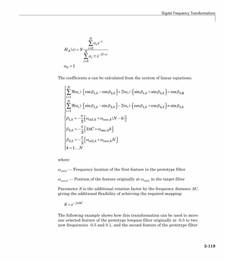
Digital Frequency Transformations
H z S
z
zA
ii
i
N
iN i
i
N( ) =
±
=
−
=
− +
=
∑
∑
0
0
0 1
The coefficients α can be calculated from the system of linear equations:
ℜ ⋅ −⎡⎣ ⎤⎦ + ℑ ⋅ +⎡⎣ ⎤⎦ =( ) cos cos ( ) sin sin cos, , , , , i k k i k k1 2 1 2 3 kki
N
i k k i k k
=∑
ℜ ⋅ −⎡⎣ ⎤⎦ − ℑ ⋅ +⎡⎣ ⎤⎦
1
1 2 1 2( ) sin sin ( ) cos cos, , , , ==
= − + −⎡⎣ ⎤⎦
= − +
=∑ sin
( )
,
, , ,
,
31
1
2
2
22
ki
N
k old k new k
k n
N k
CΔ eew k
k old k new k
k
N
k N
,
, , ,
⎡⎣ ⎤⎦
= − +⎡⎣ ⎤⎦=
⎧
⎨
⎪⎪⎪⎪⎪⎪⎪
⎩
⎪⎪⎪⎪⎪⎪⎪
3 2
1
where
ωold,k— Frequency location of the first feature in the prototype filter
ωnew,k— Position of the feature originally at ωold,k in the target filter
Parameter S is the additional rotation factor by the frequency distance ΔC,giving the additional flexibility of achieving the required mapping:
S e j C= − Δ
The following example shows how this transformation can be used to moveone selected feature of the prototype lowpass filter originally at -0.5 to twonew frequencies -0.5 and 0.1, and the second feature of the prototype filter
3-119
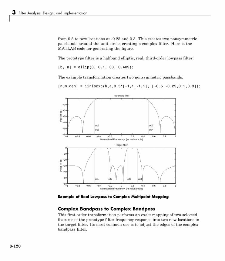
3 Filter Analysis, Design, and Implementation
from 0.5 to new locations at -0.25 and 0.3. This creates two nonsymmetricpassbands around the unit circle, creating a complex filter. Here is theMATLAB code for generating the figure.
The prototype filter is a halfband elliptic, real, third-order lowpass filter:
[b, a] = ellip(3, 0.1, 30, 0.409);
The example transformation creates two nonsymmetric passbands:
[num,den] = iirlp2xc(b,a,0.5*[-1,1,-1,1], [-0.5,-0.25,0.1,0.3]);
−1 −0.8 −0.6 −0.4 −0.2 0 0.2 0.4 0.6 0.8 1−60
−50
−40
−30
−20
−10
0Prototype filter
|H(ω
)|in
dB
Normalized Frequency (×π rad/sample)
ωo1 ωo2
ωo3 ωo4
−1 −0.8 −0.6 −0.4 −0.2 0 0.2 0.4 0.6 0.8 1−60
−50
−40
−30
−20
−10
0Target filter
|H(ω
)| in
dB
Normalized Frequency (×π rad/sample)
ωt1 ωt2 ωt3 ωt4
Example of Real Lowpass to Complex Multipoint Mapping
Complex Bandpass to Complex BandpassThis first-order transformation performs an exact mapping of two selectedfeatures of the prototype filter frequency response into two new locations inthe target filter. Its most common use is to adjust the edges of the complexbandpass filter.
3-120

Digital Frequency Transformations
H zz
zA( )
( )= −−
−
−
1
1
with α and β are given by
=
− − −
−
sin (( ) ( ))
sin ((
, , , ,
,
4
4
2 1 2 1
2
old old new new
old old,, , ,
( )
(
) ( ))
, ,
,
1 2 1
2 1
2
+ −
=
=
− −
− −
new new
j
j
e
e
old old
new neew, )1
where
ωold,1— Frequency location of the first feature in the prototype filter
ωold,2— Frequency location of the second feature in the prototype filter
ωnew,1— Position of the feature originally at ωold,1 in the target filter
ωnew,2— Position of the feature originally at ωold,2 in the target filter
The following example shows how this transformation can be used to modifythe position of the passband of the prototype filter, either real or complex. Inthe example below the prototype filter passband spanned from 0.5 to 0.75.It was converted to having a passband between -0.5 and 0.1. Here is theMATLAB code for generating the figure.
The prototype filter is a halfband elliptic, real, third-order lowpass filter:
[b, a] = ellip(3, 0.1, 30, 0.409);
The example transformation creates a passband from 0.25 to 0.75:
[num,den] = iirbpc2bpc(b, a, [0.25, 0.75], [-0.5, 0.1]);
3-121

3 Filter Analysis, Design, and Implementation
−1 −0.8 −0.6 −0.4 −0.2 0 0.2 0.4 0.6 0.8 1−60
−50
−40
−30
−20
−10
0Prototype filter
|H(ω
)|in
dB
Normalized Frequency (×π rad/sample)
ωo1 ωo2
−1 −0.8 −0.6 −0.4 −0.2 0 0.2 0.4 0.6 0.8 1−60
−50
−40
−30
−20
−10
0Target filter
|H(ω
)| in
dB
Normalized Frequency (×π rad/sample)
ωt1 ωt2
Example of Complex Bandpass to Complex Bandpass Mapping
3-122

Digital Filter Design Block
Digital Filter Design Block
In this section...
“Overview of the Digital Filter Design Block” on page 3-123
“Select a Filter Design Block” on page 3-124
“Create a Lowpass Filter in Simulink” on page 3-126
“Create a Highpass Filter in Simulink” on page 3-127
“Filter High-Frequency Noise in Simulink” on page 3-128
Overview of the Digital Filter Design BlockYou can use the Digital Filter Design block to design and implement a digitalfilter. The filter you design can filter single-channel or multichannel signals.The Digital Filter Design block is ideal for simulating the numerical behaviorof your filter on a floating-point system, such as a personal computer or DSPchip. You can use the Simulink Coder product to generate C code from yourfilter block. For more information on generating C code from models, see“Understanding Code Generation” on page 9-2.
Filter Design and AnalysisYou perform all filter design and analysis within the Filter Design andAnalysis Tool (FDATool) GUI, which opens when you double-click the DigitalFilter Design block. FDATool provides extensive filter design parameters andanalysis tools such as pole-zero and impulse response plots.
Filter ImplementationOnce you have designed your filter using FDATool, the block automaticallyrealizes the filter using the filter structure you specify. You can then usethe block to filter signals in your model. You can also fine-tune the filter bychanging the filter specification parameters during a simulation. The outputsof the Digital Filter Design block numerically match the outputs of the DSPSystem Toolbox filter function and the MATLAB filter function.
3-123
3 Filter Analysis, Design, and Implementation
Saving, Exporting, and Importing FiltersThe Digital Filter Design block allows you to save the filters you design,export filters (to the MATLAB workspace, MAT-files, etc.), and import filtersdesigned elsewhere.
To learn how to save your filter designs, see “Saving and OpeningFilter Design Sessions” on page 13-38 in the Signal Processing Toolboxdocumentation. To learn how to import and export your filter designs, see“Import and Export Quantized Filters” on page 3-54.
Note You can use the Digital Filter Design block to design and implement afilter. To implement a pre-designed filter, use the Digital Filter block. Bothblocks implement a filter design in the same manner and have the samebehavior during simulation and code generation.
See the Digital Filter Design block reference page for more information. Forinformation on choosing between the Digital Filter Design block and the FilterRealization Wizard, see “Select a Filter Design Block” on page 3-124.
Select a Filter Design BlockThis section explains the similarities and differences between the DigitalFilter Design and Filter Realization Wizard blocks.
SimilaritiesThe Digital Filter Design block and Filter Realization Wizard are similarin the following ways:
• Filter design and analysis options — Both blocks use the Filter Design andAnalysis Tool (FDATool) GUI for filter design and analysis.
• Output values — If the output of both blocks is double-precision floatingpoint, single-precision floating point, or fixed point, the output values ofboth blocks numerically match the output of the filter method of thedfilt object.
3-124

Digital Filter Design Block
DifferencesThe Digital Filter Design block and Filter Realization Wizard handle thefollowing things differently:
• Supported filter structures — Both blocks support many of the samebasic filter structures, but the Filter Realization Wizard supports morestructures than the Digital Filter Design block. This is because the blockcan implement filters using Sum, Gain, and Delay blocks. See the FilterRealization Wizard and Digital Filter Design block reference pages for alist of all the structures they support.
• Data type support — The Filter Realization Wizard block supports single-and double-precision floating-point computation for all filter structures andfixed-point computation for some filter structures. The Digital Filter Designblock only supports single- and double-precision floating-point computation.
• Block versus Wizard — The Digital Filter Design block is the filter itself,but the Filter Realization Wizard block just enables you to create newfilters and put them in an existing model. Thus, the Filter RealizationWizard is not a block that processes data in your model, it is a wizard thatgenerates filter blocks (or subsystems) which you can then use to processdata in your model.
When to Use Each BlockThe following are specific situations where only the Digital Filter Designblock or the Filter Realization Wizard is appropriate.
• Digital Filter Design
- Use to simulate single- and double-precision floating-point filters.
- Use to generate highly optimized ANSI® C code that implementsfloating-point filters for embedded systems.
• Filter Realization Wizard
- Use to simulate numerical behavior of fixed-point filters in a DSP chip,a field-programmable gate array (FPGA), or an application-specificintegrated circuit (ASIC).
- Use to simulate single- and double-precision floating-point filters withstructures that the Digital Filter Design block does not support.
3-125

3 Filter Analysis, Design, and Implementation
- Use to visualize the filter structure, as the block can build the filterfrom Sum, Gain, and Delay blocks.
- Use to rapidly generate multiple filter blocks.
See “Filter Realization Wizard” on page 3-134 and the Filter RealizationWizard block reference page for information.
Create a Lowpass Filter in SimulinkYou can use the Digital Filter Design block to design and implement a digitalFIR or IIR filter. In this topic, you use it to create an FIR lowpass filter:
1 Open Simulink and create a new model file.
2 From the DSP System Toolbox Filtering library, and then from the FilterImplementations library, click-and-drag a Digital Filter Design block intoyour model.
3 Double-click the Digital Filter Design block.
The Filter Design and Analysis Tool (FDATool) GUI opens.
4 Set the parameters as follows, and then click OK:
• Response Type = Lowpass
• Design Method = FIR, Equiripple
• Filter Order = Minimum order
• Units = Normalized (0 to 1)
• wpass = 0.2
• wstop = 0.5
5 Click Design Filter at the bottom of the GUI to design the filter.
Your Digital Filter Design block now represents a filter with theparameters you specified.
6 From the Edit menu, select Convert Structure.
The Convert Structure dialog box opens.
3-126

Digital Filter Design Block
7 Select Direct-Form FIR Transposed and click OK.
8 Rename your block Digital Filter Design - Lowpass.
The Digital Filter Design block now represents a lowpass filter with aDirect-Form FIR Transposed structure. The filter passes all frequencies upto 20% of the Nyquist frequency (half the sampling frequency), and stopsfrequencies greater than or equal to 50% of the Nyquist frequency as definedby the wpass and wstop parameters. In the next topic, “Create a HighpassFilter in Simulink” on page 3-127, you use a Digital Filter Design blockto create a highpass filter. For more information about implementing apre-designed filter, see “Digital Filter Block” on page 3-147.
Create a Highpass Filter in SimulinkIn this topic, you create a highpass filter using the Digital Filter Design block:
1 If the model you created in “Create a Lowpass Filter in Simulink” on page3-126 is not open on your desktop, you can open an equivalent model bytyping
ex_filter_ex4
at the MATLAB command prompt.
2 From the DSP System Toolbox Filtering library, and then from the FilterImplementations library, click-and-drag a second Digital Filter Designblock into your model.
3 Double-click the Digital Filter Design block.
The Filter Design and Analysis Tool (FDATool) GUI opens.
4 Set the parameters as follows:
• Response Type = Highpass
• Design Method = FIR, Equiripple
• Filter Order = Minimum order
• Units = Normalized (0 to 1)
• wstop = 0.2
3-127
3 Filter Analysis, Design, and Implementation
• wpass = 0.5
5 Click theDesign Filter button at the bottom of the GUI to design the filter.
Your Digital Filter Design block now represents a filter with theparameters you specified.
6 In the Edit menu, select Convert Structure.
The Convert Structure dialog box opens.
7 Select Direct-Form FIR Transposed and click OK.
8 Rename your block Digital Filter Design - Highpass .
The block now implements a highpass filter with a direct form FIR transposestructure. The filter passes all frequencies greater than or equal to 50% ofthe Nyquist frequency (half the sampling frequency), and stops frequenciesless than or equal to 20% of the Nyquist frequency as defined by the wpassand wstop parameters. This highpass filter is the opposite of the lowpassfilter described in “Create a Lowpass Filter in Simulink” on page 3-126. Thehighpass filter passes the frequencies stopped by the lowpass filter, andstops the frequencies passed by the lowpass filter. In the next topic, “FilterHigh-Frequency Noise in Simulink” on page 3-128, you use these DigitalFilter Design blocks to create a model capable of removing high frequencynoise from a signal. For more information about implementing a pre-designedfilter, see “Digital Filter Block” on page 3-147.
Filter High-Frequency Noise in SimulinkIn the previous topics, you used Digital Filter Design blocks to create FIRlowpass and highpass filters. In this topic, you use these blocks to build amodel that removes high frequency noise from a signal. In this model, youuse the highpass filter, which is excited using a uniform random signal, tocreate high-frequency noise. After you add this noise to a sine wave, you usethe lowpass filter to filter out the high-frequency noise:
1 If the model you created in “Create a Highpass Filter in Simulink” on page3-127 is not open on your desktop, you can open an equivalent model bytyping
3-128
Digital Filter Design Block
ex_filter_ex5
at the MATLAB command prompt.
2 Click-and-drag the following blocks into your model.
Block Library Quantity
Add Simulink Math Operationslibrary
1
Random Source Sources 1
Sine Wave Sources 1
Time Scope Sinks 1
3 Set the parameters for these blocks as indicated in the following table.Leave the parameters not listed in the table at their default settings.
Parameter Settings for the Other Blocks
Block Parameter Setting
Add • Icon shape = rectangular
• List of signs = ++
RandomSource
• Source type = = Uniform
• Minimum = 0
• Maximum = 4
• Sample mode = Discrete
• Sample time = 1/1000
• Samples per frame = 50
3-129

3 Filter Analysis, Design, and Implementation
Parameter Settings for the Other Blocks (Continued)
Block Parameter Setting
Sine Wave • Frequency (Hz) = 75
• Sample time = 1/1000
• Samples per frame = 50
Time Scope • File > Number of Input Ports > 3
• File > Configuration ...
– Open the Visuals:Time Domain Options dialogand set Time span = One frame period
4 Connect the blocks as shown in the following figure. You might need toresize some of the blocks to accomplish this task.
5 From the Simulation menu, selectModel Configuration Parameters.
3-130

Digital Filter Design Block
The Configuration Parameters dialog box opens.
6 In the Solver pane, set the parameters as follows, and then click OK:
• Start time = 0
• Stop time = 5
• Type = Fixed-step
• Solver = Discrete (no continuous states)
7 In the model window, from the Simulation menu, choose Run.
The model simulation begins and the scope displays the three input signals.
8 After simulation is complete, select View > Legend from the TimeScope menu. The legend appears in the Time Scope window. You canclick-and-drag it anywhere on the scope display. To change the channelnames, double-click inside the legend and replace the default channelnames with the following:
• Add = Noisy Sine Wave
• Digital Filter Design – Lowpass = Filtered Noisy Sine Wave
• Sine Wave = Original Sine Wave
In the next step, you will set the color, style, and marker of each channel.
9 In the Time Scope window, select View > Line Properties, and set thefollowing:
Line Style Marker Color
Noisy Sine Wave - None Black
Filtered NoisySine Wave
- diamond Red
Original SineWave
None * Blue
10 The Time Scope display should now appear as follows:
3-131
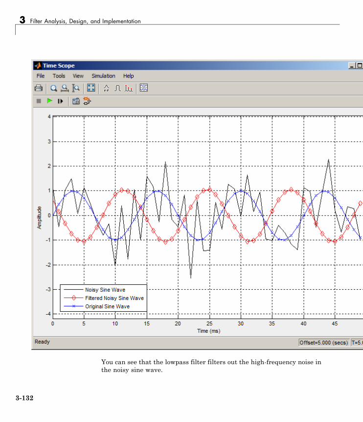
3 Filter Analysis, Design, and Implementation
You can see that the lowpass filter filters out the high-frequency noise inthe noisy sine wave.
3-132

Digital Filter Design Block
You have now used Digital Filter Design blocks to build a model that removeshigh frequency noise from a signal. For more information about these blocks,see the Digital Filter Design block reference page. For information on anotherblock capable of designing and implementing filters, see “Filter RealizationWizard” on page 3-134. To learn how to save your filter designs, see “Savingand Opening Filter Design Sessions” on page 13-38 in the Signal ProcessingToolbox documentation. To learn how to import and export your filter designs,see “Import and Export Quantized Filters” on page 3-54 in the DSP SystemToolbox documentation.
3-133

3 Filter Analysis, Design, and Implementation
Filter Realization Wizard
In this section...
“Overview of the Filter Realization Wizard” on page 3-134
“Design and Implement a Fixed-Point Filter in Simulink” on page 3-134
“Set the Filter Structure and Number of Filter Sections” on page 3-143
“Optimize the Filter Structure” on page 3-144
Overview of the Filter Realization WizardThe Filter Realization Wizard is another DSP System Toolbox block thatcan be used to design and implement digital filters. You can use this tool tofilter single-channel floating-point or fixed-point signals. Like the DigitalFilter Design block, double-clicking a Filter Realization Wizard block opensFDATool. Unlike the Digital Filter Design block, the Filter RealizationWizard starts FDATool with the Realize Model panel selected. This panel isoptimized for use with DSP System Toolbox software.
For more information, see the Filter Realization Wizard block reference page.For information on choosing between the Digital Filter Design block and theFilter Realization Wizard, see “Select a Filter Design Block” on page 3-124.
Design and Implement a Fixed-Point Filter in SimulinkIn this section, a tutorial guides you through creating a fixed-point filter withthe Filter Realization Wizard. You will use the Filter Realization Wizard toremove noise from a signal. This tutorial has the following parts:
• “Part 1 — Create a Signal with Added Noise” on page 3-135
• “Part 2 — Create a Fixed-Point Filter with the Filter Realization Wizard”on page 3-136
• “Part 3 — Build a Model to Filter a Signal” on page 3-141
• “Part 4 — Examine Filtering Results” on page 3-142
3-134
Filter Realization Wizard
Part 1 — Create a Signal with Added NoiseIn this section of the tutorial, you will create a signal with added noise. Laterin the tutorial, you will filter this signal with a fixed-point filter that youdesign with the Filter Realization Wizard.
1 Type
load mtlbsoundsc(mtlb,Fs)
at the MATLAB command line. You should hear a voice say “MATLAB.”This is the signal to which you will add noise.
2 Create a noise signal by typing
noise = cos(2*pi*3*Fs/8*(0:length(mtlb)-1)/Fs)';
at the command line. You can hear the noise signal by typing
soundsc(noise,Fs)
3 Add the noise to the original signal by typing
u = mtlb + noise;
at the command line.
4 Scale the signal with noise by typing
u = u/max(abs(u));
at the command line. You scale the signal to try to avoid overflows later on.You can hear the scaled signal with noise by typing
soundsc(u,Fs)
5 View the scaled signal with noise by typing
spectrogram(u,256,[],[],Fs);colorbar
at the command line.
The spectrogram appears as follows.
3-135
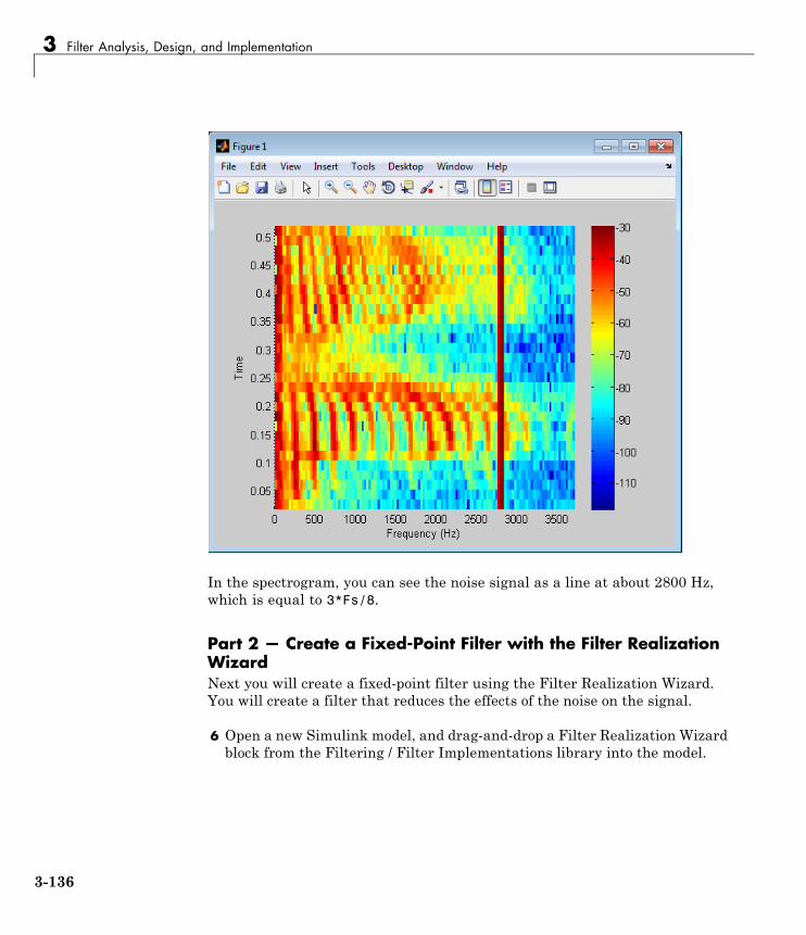
3 Filter Analysis, Design, and Implementation
In the spectrogram, you can see the noise signal as a line at about 2800 Hz,which is equal to 3*Fs/8.
Part 2 — Create a Fixed-Point Filter with the Filter RealizationWizardNext you will create a fixed-point filter using the Filter Realization Wizard.You will create a filter that reduces the effects of the noise on the signal.
6 Open a new Simulink model, and drag-and-drop a Filter Realization Wizardblock from the Filtering / Filter Implementations library into the model.
3-136

Filter Realization Wizard
Note You do not have to place a Filter Realization Wizard block in amodel in order to use it. You can open the GUI from within a library.However, for purposes of this tutorial, we will keep the Filter RealizationWizard block in the model.
7 Double-click the Filter Realization Wizard block in your model. TheRealize Model panel of the Filter Design and Analysis Tool (FDATool)appears.
8 Click the Design Filter button ( ) on the bottom left of FDATool. Thisbrings forward the Design filter panel of the tool.
9 Set the following fields in the Design filter panel:
• Set Design Method to IIR -- Constrained Least Pth-norm
• Set Fs to Fs
• Set Fpass to 0.2*Fs
• Set Fstop to 0.25*Fs
• Set Max pole radius to 0.8
• Click the Design Filter button
The Design filter panel should now appear as follows.
3-137
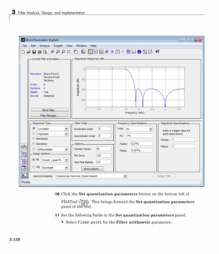
3 Filter Analysis, Design, and Implementation
10 Click the Set quantization parameters button on the bottom left of
FDATool ( ). This brings forward the Set quantization parameterspanel of the tool.
11 Set the following fields in the Set quantization parameters panel:
• Select Fixed-point for the Filter arithmetic parameter.
3-138
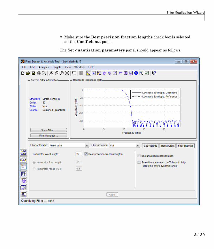
Filter Realization Wizard
• Make sure the Best precision fraction lengths check box is selectedon the Coefficients pane.
The Set quantization parameters panel should appear as follows.
3-139
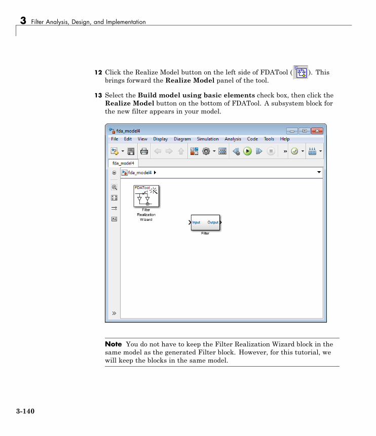
3 Filter Analysis, Design, and Implementation
12 Click the Realize Model button on the left side of FDATool ( ). Thisbrings forward the Realize Model panel of the tool.
13 Select the Build model using basic elements check box, then click theRealize Model button on the bottom of FDATool. A subsystem block forthe new filter appears in your model.
Note You do not have to keep the Filter Realization Wizard block in thesame model as the generated Filter block. However, for this tutorial, wewill keep the blocks in the same model.
3-140
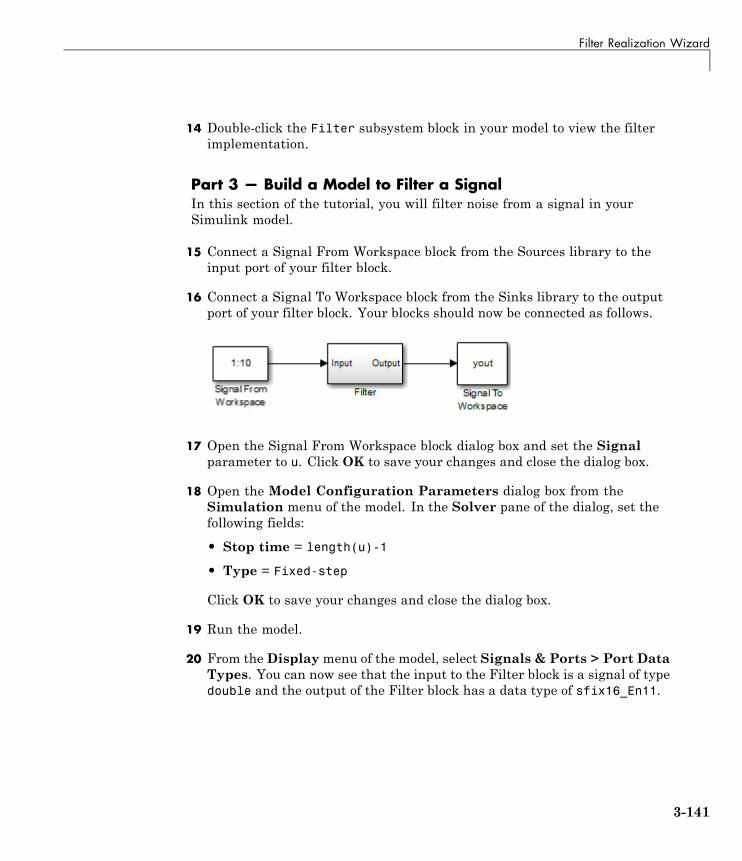
Filter Realization Wizard
14 Double-click the Filter subsystem block in your model to view the filterimplementation.
Part 3 — Build a Model to Filter a SignalIn this section of the tutorial, you will filter noise from a signal in yourSimulink model.
15 Connect a Signal From Workspace block from the Sources library to theinput port of your filter block.
16 Connect a Signal To Workspace block from the Sinks library to the outputport of your filter block. Your blocks should now be connected as follows.
17 Open the Signal From Workspace block dialog box and set the Signalparameter to u. Click OK to save your changes and close the dialog box.
18 Open the Model Configuration Parameters dialog box from theSimulation menu of the model. In the Solver pane of the dialog, set thefollowing fields:
• Stop time = length(u)-1
• Type = Fixed-step
Click OK to save your changes and close the dialog box.
19 Run the model.
20 From the Displaymenu of the model, select Signals & Ports > Port DataTypes. You can now see that the input to the Filter block is a signal of typedouble and the output of the Filter block has a data type of sfix16_En11.
3-141
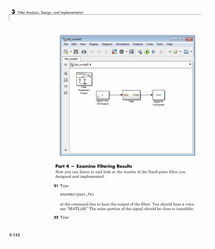
3 Filter Analysis, Design, and Implementation
Part 4 — Examine Filtering ResultsNow you can listen to and look at the results of the fixed-point filter youdesigned and implemented.
21 Type
soundsc(yout,Fs)
at the command line to hear the output of the filter. You should hear a voicesay “MATLAB.” The noise portion of the signal should be close to inaudible.
22 Type
3-142

Filter Realization Wizard
figurespectrogram(yout,256,[],[],Fs);colorbar
at the command line.
From the colorbars at the side of the input and output spectrograms, you cansee that the noise has been reduced by about 40 dB.
Set the Filter Structure and Number of Filter SectionsThe Current Filter Information region of FDATool shows the structureand the number of second-order sections in your filter.
Change the filter structure and number of filter sections of your filter asfollows:
• Select Convert Structure from the Edit menu to open the ConvertStructure dialog box. For details, see “Converting to a New Structure” inthe Signal Processing Toolbox documentation.
3-143
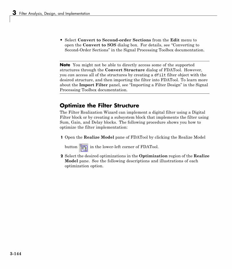
3 Filter Analysis, Design, and Implementation
• Select Convert to Second-order Sections from the Edit menu toopen the Convert to SOS dialog box. For details, see “Converting toSecond-Order Sections” in the Signal Processing Toolbox documentation.
Note You might not be able to directly access some of the supportedstructures through the Convert Structure dialog of FDATool. However,you can access all of the structures by creating a dfilt filter object with thedesired structure, and then importing the filter into FDATool. To learn moreabout the Import Filter panel, see “Importing a Filter Design” in the SignalProcessing Toolbox documentation.
Optimize the Filter StructureThe Filter Realization Wizard can implement a digital filter using a DigitalFilter block or by creating a subsystem block that implements the filter usingSum, Gain, and Delay blocks. The following procedure shows you how tooptimize the filter implementation:
1 Open the Realize Model pane of FDATool by clicking the Realize Model
button in the lower-left corner of FDATool.
2 Select the desired optimizations in the Optimization region of the RealizeModel pane. See the following descriptions and illustrations of eachoptimization option.
3-144

Filter Realization Wizard
• Optimize for zero gains— Remove zero-gain paths.
• Optimize for unity gains — Substitute gains equal to one with a wire(short circuit).
• Optimize for negative gains— Substitute gains equal to -1 with a wire(short circuit), and change the corresponding sums to subtractions.
• Optimize delay chains— Substitute any delay chain made up of n unitdelays with a single delay by n.
• Optimize for unity scale values—Remove all scale value multiplicationsby 1 from the filter structure.
The following diagram illustrates the results of each of these optimizations.
3-145

3 Filter Analysis, Design, and Implementation
3-146
Digital Filter Block
Digital Filter Block
In this section...
“Overview of the Digital Filter Block” on page 3-147
“Implement a Lowpass Filter in Simulink” on page 3-148
“Implement a Highpass Filter in Simulink” on page 3-149
“Filter High-Frequency Noise in Simulink” on page 3-150
“Specify Static Filters” on page 3-155
“Specify Time-Varying Filters” on page 3-155
“Specify the SOS Matrix (Biquadratic Filter Coefficients)” on page 3-157
Overview of the Digital Filter BlockYou can use the Digital Filter block to implement digital FIR and IIR filtersin your models. Use this block if you have already performed the design andanalysis and know your desired filter coefficients. You can use this block tofilter single-channel and multichannel signals, and to simulate floating-pointand fixed-point filters. Then, you can use the Simulink Coder product togenerate highly optimized C code from your filter block.
To implement a filter with the Digital Filter block, you must provide thefollowing basic information about the filter:
• Whether the filter transfer function is FIR with all zeros, IIR with all poles,or IIR with poles and zeros
• The desired filter structure
• The filter coefficients
Note Use the Digital Filter Design block to design and implement a filter.Use the Digital Filter block to implement a pre-designed filter. Both blocksimplement a filter in the same manner and have the same behavior duringsimulation and code generation.
3-147

3 Filter Analysis, Design, and Implementation
Implement a Lowpass Filter in SimulinkYou can use the Digital Filter block to implement a digital FIR or IIR filter.In this topic, you use it to implement an FIR lowpass filter:
1 Define the lowpass filter coefficients in the MATLAB workspace by typing
lopassNum = [-0.0021 -0.0108 -0.0274 -0.0409 -0.0266 0.03740.1435 0.2465 0.2896 0.2465 0.1435 0.0374 -0.0266 -0.0409-0.0274 -0.0108 -0.0021];
2 Open Simulink and create a new model file.
3 From the DSP System Toolbox Filtering>Filter Implementations library,click-and-drag a Digital Filter block into your model.
4 Double-click the Digital Filter block. Set the block parameters as follows,and then click OK:
• Coefficient source = Dialog parameters
• Transfer function type = FIR (all zeros)
• Filter structure = Direct form transposed
• Numerator coefficients = lopassNum
• Input processing = Columns as channels (frame based)
• Initial conditions = 0
Note that you can provide the filter coefficients in several ways:
• Type in a variable name from the MATLAB workspace, such aslopassNum.
• Type in filter design commands from Signal Processing Toolbox softwareor DSP System Toolbox software, such as fir1(5, 0.2, 'low').
• Type in a vector of the filter coefficient values.
5 Rename your block Digital Filter - Lowpass.
The Digital Filter block in your model now represents a lowpass filter. In thenext topic, “Implement a Highpass Filter in Simulink” on page 3-149, you usea Digital Filter block to implement a highpass filter. For more information
3-148

Digital Filter Block
about the Digital Filter block, see the Digital Filter block reference page. Formore information about designing and implementing a new filter, see “DigitalFilter Design Block” on page 3-123.
Implement a Highpass Filter in SimulinkIn this topic, you implement an FIR highpass filter using the Digital Filterblock:
1 If the model you created in “Implement a Lowpass Filter in Simulink”on page 3-148 is not open on your desktop, you can open an equivalentmodel by typing
ex_filter_ex1
at the MATLAB command prompt.
2 Define the highpass filter coefficients in the MATLAB workspace by typing
hipassNum = [-0.0051 0.0181 -0.0069 -0.0283 -0.0061 ...0.0549 0.0579 -0.0826 -0.2992 0.5946 -0.2992 -0.0826 ...0.0579 0.0549 -0.0061 -0.0283 -0.0069 0.0181 -0.0051];
3 From the DSP System Toolbox Filtering library, and then from the FilterImplementations library, click-and-drag a Digital Filter block into yourmodel.
4 Double-click the Digital Filter block. Set the block parameters as follows,and then click OK:
• Coefficient source = Dialog parameters
• Transfer function type = FIR (all zeros)
• Filter structure = Direct form transposed
• Numerator coefficients = hipassNum
• Input processing = Columns as channels (frame based)
• Initial conditions = 0
You can provide the filter coefficients in several ways:
3-149

3 Filter Analysis, Design, and Implementation
• Type in a variable name from the MATLAB workspace, such ashipassNum.
• Type in filter design commands from Signal Processing Toolbox softwareor DSP System Toolbox software, such as fir1(5, 0.2, 'low').
• Type in a vector of the filter coefficient values.
5 Rename your block Digital Filter - Highpass.
You have now successfully implemented a highpass filter. In the next topic,“Filter High-Frequency Noise in Simulink” on page 3-150, you use theseDigital Filter blocks to create a model capable of removing high frequencynoise from a signal. For more information about designing and implementinga new filter, see “Digital Filter Design Block” on page 3-123.
Filter High-Frequency Noise in SimulinkIn the previous topics, you used Digital Filter blocks to implement FIRlowpass and highpass filters. In this topic, you use these blocks to build amodel that removes high frequency noise from a signal. In this model, youuse the highpass filter, which is excited using a uniform random signal, tocreate high-frequency noise. After you add this noise to a sine wave, you usethe lowpass filter to filter out the high-frequency noise:
1 If the model you created in “Implement a Highpass Filter in Simulink”on page 3-149 is not open on your desktop, you can open an equivalentmodel by typing
ex_filter_ex2
at the MATLAB command prompt.
2 If you have not already done so, define the lowpass and highpass filtercoefficients in the MATLAB workspace by typing
lopassNum = [-0.0021 -0.0108 -0.0274 -0.0409 -0.0266 ...0.0374 0.1435 0.2465 0.2896 0.2465 0.1435 0.0374 ...-0.0266 -0.0409 -0.0274 -0.0108 -0.0021];hipassNum = [-0.0051 0.0181 -0.0069 -0.0283 -0.0061 ...0.0549 0.0579 -0.0826 -0.2992 0.5946 -0.2992 -0.0826 ...0.0579 0.0549 -0.0061 -0.0283 -0.0069 0.0181 -0.0051];
3-150

Digital Filter Block
3 Click-and-drag the following blocks into your model file.
Block Library Quantity
Add Simulink / Math Operationslibrary
1
Random Source Sources 1
Sine Wave Sources 1
Time Scope Sinks 1
4 Set the parameters for the rest of the blocks as indicated in the followingtable. For any parameters not listed in the table, leave them at theirdefault settings.
Block Parameter Setting
Add • Icon shape = rectangular
• List of signs = ++
Random Source • Source type = Uniform
• Minimum = 0
• Maximum = 4
• Sample mode = Discrete
• Sample time = 1/1000
• Samples per frame = 50
Sine Wave • Frequency (Hz) = 75
• Sample time = 1/1000
• Samples per frame = 50
Time Scope • File > Number of Input Ports > 3
• File > Configuration ...
– Open the Visuals:Time Domain Optionsdialog and set Time span = One frameperiod
3-151
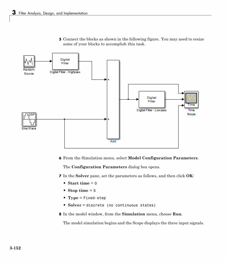
3 Filter Analysis, Design, and Implementation
5 Connect the blocks as shown in the following figure. You may need to resizesome of your blocks to accomplish this task.
6 From the Simulation menu, selectModel Configuration Parameters.
The Configuration Parameters dialog box opens.
7 In the Solver pane, set the parameters as follows, and then click OK:
• Start time = 0
• Stop time = 5
• Type = Fixed-step
• Solver = discrete (no continuous states)
8 In the model window, from the Simulation menu, choose Run.
The model simulation begins and the Scope displays the three input signals.
3-152

Digital Filter Block
9 After simulation is complete, select View > Legend from the TimeScope menu. The legend appears in the Time Scope window. You canclick-and-drag it anywhere on the scope display. To change the channelnames, double-click inside the legend and replace the current numberedchannel names with the following:
• Add = Noisy Sine Wave
• Digital Filter – Lowpass = Filtered Noisy Sine Wave
• Sine Wave = Original Sine Wave
In the next step, you will set the color, style, and marker of each channel.
10 In the Time Scope window, select View > Line Properties, and set thefollowing:
Line Style Marker Color
Noisy Sine Wave - None Black
Filtered NoisySine Wave
- diamond Red
Original SineWave
None * Blue
11 The Time Scope display should now appear as follows:
You can see that the lowpass filter filters out the high-frequency noise inthe noisy sine wave.
3-153

3 Filter Analysis, Design, and Implementation
3-154
Digital Filter Block
You have now used Digital Filter blocks to build a model that removes highfrequency noise from a signal. For more information about designing andimplementing a new filter, see “Digital Filter Design Block” on page 3-123.
Specify Static FiltersYou can use the Digital Filter block to specify a static filter by setting theCoefficient source parameter to Specify via dialog. Depending on thefilter structure, you need to enter your filter coefficients into one or more ofthe following parameters. The block disables all the irrelevant parameters.To see which of these parameters correspond to each filter structure, see“Supported Filter Structures” in DSP System Toolbox Reference:
• Numerator coefficients — Column or row vector of numeratorcoefficients, [b0, b1, b2, ..., bn].
• Denominator coefficients — Column or row vector of denominatorcoefficients, [a0, a1, a2, ..., am].
• Reflection coefficients— Column or row vector of reflection coefficients,[k1, k2, ..., kn].
• SOS matrix (Mx6) — M-by-6 SOS matrix. You can also use the BiquadFilter block to create a static biquadratic IIR filter.
• Scale values — Scalar or vector of M+1 scale values to be used betweenSOS stages.
Tuning the Filter Coefficient Values During SimulationTo change the static filter coefficients during simulation, double-click theblock, type in the new vector(s) of filter coefficients, and click OK. You cannotchange the filter order, so you cannot change the number of elements in thevector(s) of filter coefficients.
Specify Time-Varying Filters
Note This block does not support time-varying Biquadratic (SOS) filters.
3-155

3 Filter Analysis, Design, and Implementation
Time-varying filters are filters whose coefficients change with time. Youcan specify a time-varying filter that changes once per frame or once persample and you can filter multiple channels with each filter. However, youcannot apply different filters to each channel; all channels must be filteredwith the same filter.
To specify a time-varying filter:
1 Set the Coefficient source parameter to Input port(s), which enablesextra block input ports for the time-varying filter coefficients.
2 Set the Coefficient update rate parameter to One filter per frameor One filter per sample depending on how often you want to updatethe filter coefficients.
3 Provide vectors of numerator, denominator, or reflection coefficients to theblock input ports for filter coefficients. The series of vectors must arrive attheir ports at a specific rate, and must be of certain lengths.
4 Select or clear the First denominator coefficient = 1, remove a0 termin the structure parameter depending on whether your first denominatorcoefficient is always 1. To learn more, see “Removing the a0 Term in theFilter Structure” on page 3-156.
Removing the a0 Term in the Filter StructureWhen you know that the first denominator filter coefficient (a0) is always 1for your time-varying filter, select the First denominator coefficient = 1,remove a0 term in the structure parameter. Selecting this parameterreduces the number of computations the block must make to produce theoutput (the block omits the 1 / a0 term in the filter structure, as illustratedin the following figure). The block output is invalid if you select thisparameter when the first denominator filter coefficient is not always 1 foryour time-varying filter. Note that the block ignores the First denominatorcoefficient = 1, remove a0 term in the structure parameter forfixed-point inputs, since this block does not support nonunity a0 coefficientsfor fixed-point inputs.
3-156
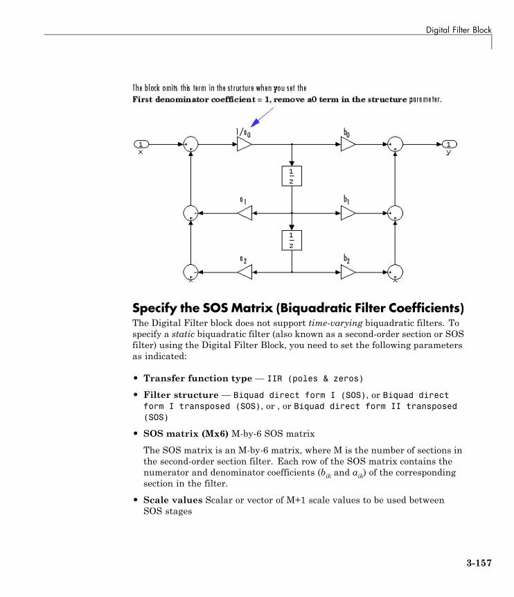
Digital Filter Block
Specify the SOS Matrix (Biquadratic Filter Coefficients)The Digital Filter block does not support time-varying biquadratic filters. Tospecify a static biquadratic filter (also known as a second-order section or SOSfilter) using the Digital Filter Block, you need to set the following parametersas indicated:
• Transfer function type — IIR (poles & zeros)
• Filter structure — Biquad direct form I (SOS), or Biquad directform I transposed (SOS), or , or Biquad direct form II transposed(SOS)
• SOS matrix (Mx6) M-by-6 SOS matrix
The SOS matrix is an M-by-6 matrix, where M is the number of sections inthe second-order section filter. Each row of the SOS matrix contains thenumerator and denominator coefficients (bik and aik) of the correspondingsection in the filter.
• Scale values Scalar or vector of M+1 scale values to be used betweenSOS stages
3-157

3 Filter Analysis, Design, and Implementation
If you enter a scalar, the value is used as the gain value before the firstsection of the second-order filter. The rest of the gain values are set to 1.
If you enter a vector of M+1 values, each value is used for a separatesection of the filter. For example, the first element is the first gain value,the second element is the second gain value, and so on.
You can use the ss2sos and tf2sos functions from Signal Processing Toolboxsoftware to convert a state-space or transfer function description of your filterinto the second-order section description used by this block.
b b b a a ab b b a a a
b b b a a aM M M M M
01 11 21 01 11 21
02 12 22 02 12 22
0 1 2 0 1
22M
⎡
⎣
⎢⎢⎢⎢⎢
⎤
⎦
⎥⎥⎥⎥⎥
The block normalizes each row by a1i to ensure a value of 1 for the zero-delaydenominator coefficients.
Note You can also use the Biquad Filter block to implement a staticbiquadratic IIR filter.
3-158
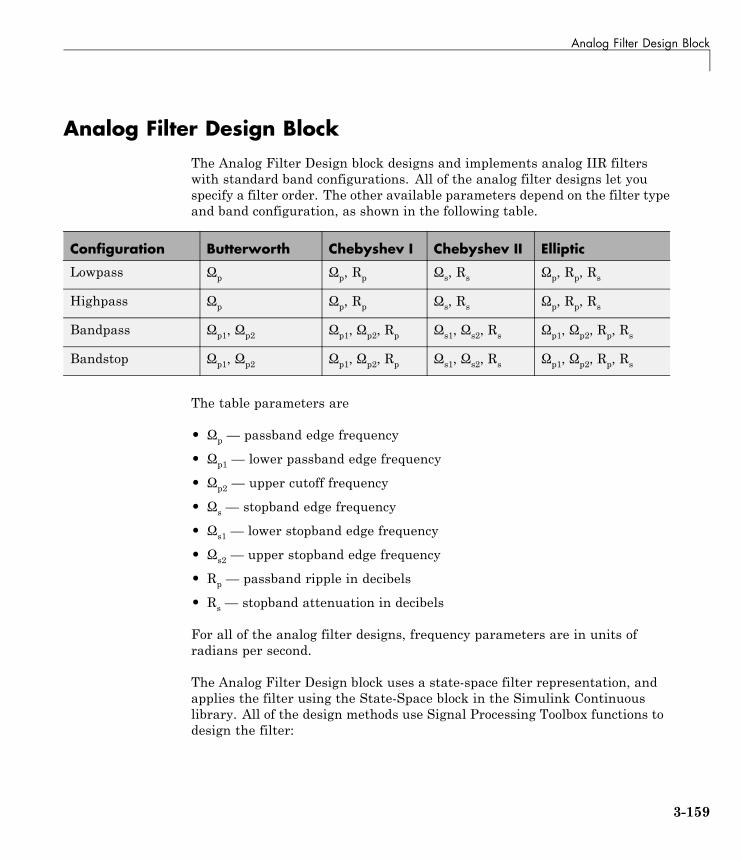
Analog Filter Design Block
Analog Filter Design BlockThe Analog Filter Design block designs and implements analog IIR filterswith standard band configurations. All of the analog filter designs let youspecify a filter order. The other available parameters depend on the filter typeand band configuration, as shown in the following table.
Configuration Butterworth Chebyshev I Chebyshev II Elliptic
Lowpass Ωp Ωp, Rp Ωs, Rs Ωp, Rp, Rs
Highpass Ωp Ωp, Rp Ωs, Rs Ωp, Rp, Rs
Bandpass Ωp1, Ωp2 Ωp1, Ωp2, Rp Ωs1, Ωs2, Rs Ωp1, Ωp2, Rp, Rs
Bandstop Ωp1, Ωp2 Ωp1, Ωp2, Rp Ωs1, Ωs2, Rs Ωp1, Ωp2, Rp, Rs
The table parameters are
• Ωp — passband edge frequency
• Ωp1 — lower passband edge frequency
• Ωp2 — upper cutoff frequency
• Ωs — stopband edge frequency
• Ωs1 — lower stopband edge frequency
• Ωs2 — upper stopband edge frequency
• Rp — passband ripple in decibels
• Rs — stopband attenuation in decibels
For all of the analog filter designs, frequency parameters are in units ofradians per second.
The Analog Filter Design block uses a state-space filter representation, andapplies the filter using the State-Space block in the Simulink Continuouslibrary. All of the design methods use Signal Processing Toolbox functions todesign the filter:
3-159

3 Filter Analysis, Design, and Implementation
• The Butterworth design uses the toolbox function butter.
• The Chebyshev type I design uses the toolbox function cheby1.
• The Chebyshev type II design uses the toolbox function cheby2.
• The elliptic design uses the toolbox function ellip.
The Analog Filter Design block is built on the filter design capabilities ofSignal Processing Toolbox software.
Note The Analog Filter Design block does not work with the Simulinkdiscrete solver, which is enabled when the Solver list is set to Discrete(no continuous states) in the Solver pane of theModel ConfigurationParameters dialog box. Select one of the continuous solvers (such as ode4)instead.
3-160

4
Adaptive Filters
Learn how to design and implement adaptive filters.
• “Overview of Adaptive Filters and Applications” on page 4-2
• “Adaptive Filters in DSP System Toolbox Software” on page 4-10
• “LMS Adaptive Filters” on page 4-14
• “RLS Adaptive Filters” on page 4-35
• “Signal Enhancement Using LMS and Normalized LMS” on page 4-41
• “Adaptive Filters in Simulink” on page 4-51
• “Selected Bibliography” on page 4-66

4 Adaptive Filters
Overview of Adaptive Filters and Applications
In this section...
“Introduction to Adaptive Filtering” on page 4-2
“Adaptive Filtering Methodology” on page 4-2
“Choosing an Adaptive Filter” on page 4-4
“System Identification” on page 4-6
“Inverse System Identification” on page 4-6
“Noise or Interference Cancellation” on page 4-7
“Prediction” on page 4-8
Introduction to Adaptive FilteringAdaptive filtering involves the changing of filter parameters (coefficients) overtime, to adapt to changing signal characteristics. Over the past three decades,digital signal processors have made great advances in increasing speed andcomplexity, and reducing power consumption. As a result, real-time adaptivefiltering algorithms are quickly becoming practical and essential for thefuture of communications, both wired and wireless.
For more detailed information about adaptive filters and adaptive filtertheory, refer to the books listed in the “Selected Bibliography” on page 4-66.
Adaptive Filtering MethodologyThis section presents a brief description of how adaptive filters work andsome of the applications where they can be useful.
Adaptive filters self learn. As the signal into the filter continues, the adaptivefilter coefficients adjust themselves to achieve the desired result, such asidentifying an unknown filter or canceling noise in the input signal. In thefigure below, the shaded box represents the adaptive filter, comprising theadaptive filter and the adaptive recursive least squares (RLS) algorithm.
4-2

Overview of Adaptive Filters and Applications
����
������� ��������������������������
�������� �����������
���������������
����������������
����������������
���������������
�
�
Block Diagram That Defines the Inputs and Output of a Generic RLS AdaptiveFilter
The next figure provides the general adaptive filter setup with inputs andoutputs.
����
������� ��������������������������
����������������
���������������
����������������
����������������
���������������
�
�
Block Diagram Defining General Adaptive Filter Algorithm Inputs andOutputs
DSP System Toolbox software includes adaptive filters of a broad range offorms, all of which can be worthwhile for specific needs. Some of the commonones are:
• Adaptive filters based on least mean squares (LMS) techniques, such asadaptfilt.lms, adaptfilt.filtxlms, and adaptfilt.nlms
• Adaptive filters based on recursive least squares (RLS) techniques. Forexample, adaptfilt.rls and adaptfilt.swrls
• Adaptive filters based on sign-data (adaptfilt.sd), sign-error(adaptfilt.se), and sign-sign (adaptfilt.ss) techniques
4-3
4 Adaptive Filters
• Adaptive filters based on lattice filters. For example, adaptfilt.gal andadaptfilt.lsl
• Adaptive filters that operate in the frequency domain, such asadaptfilt.fdaf and adaptfilt.pbufdaf.
• Adaptive filters that operate in the transform domain. Two of these are theadaptfilt.tdafdft and adaptfilt.tdafdct filters
An adaptive filter designs itself based on the characteristics of the inputsignal to the filter and a signal that represents the desired behavior of thefilter on its input.
Designing the filter does not require any other frequency response informationor specification. To define the self-learning process the filter uses, you selectthe adaptive algorithm used to reduce the error between the output signaly(k) and the desired signal d(k).
When the LMS performance criterion for e(k) has achieved its minimum valuethrough the iterations of the adapting algorithm, the adaptive filter is finishedand its coefficients have converged to a solution. Now the output from theadaptive filter matches closely the desired signal d(k). When you change theinput data characteristics, sometimes called the filter environment, the filteradapts to the new environment by generating a new set of coefficients for thenew data. Notice that when e(k) goes to zero and remains there you achieveperfect adaptation, the ideal result but not likely in the real world.
The adaptive filter functions in this toolbox implement the shaded portion ofthe figures, replacing the adaptive algorithm with an appropriate technique.To use one of the functions, you provide the input signal or signals and theinitial values for the filter.
“Adaptive Filters in DSP System Toolbox Software” on page 4-10 offersdetails about the algorithms available and the inputs required to use themin MATLAB.
Choosing an Adaptive FilterSelecting the adaptive filter that best meets your needs requires carefulconsideration. An exhaustive discussion of the criteria for selecting your
4-4
Overview of Adaptive Filters and Applications
approach is beyond the scope of this User’s Guide. However, a few guidelinescan help you make your choice.
Two main considerations frame the decision — how you plan to use the filterand the filter algorithm to use.
When you begin to develop an adaptive filter for your needs, most likely theprimary concern is whether using an adaptive filter is a cost-competitiveapproach to solving your filtering needs. Generally many areas determine thesuitability of adaptive filters (these areas are common to most filtering andsignal processing applications). Four such areas are
• Filter consistency — Does your filter performance degrade when the filtercoefficients change slightly as a result of quantization, or you switchto fixed-point arithmetic? Will excessive noise in the signal hurt theperformance of your filter?
• Filter performance — Does your adaptive filter provide sufficientidentification accuracy or fidelity, or does the filter provide sufficient signaldiscrimination or noise cancellation to meet your requirements?
• Tools — Do tools exist that make your filter development process easier?Better tools can make it practical to use more complex adaptive algorithms.
• DSP requirements — Can your filter perform its job within the constraintsof your application? Does your processor have sufficient memory,throughput, and time to use your proposed adaptive filtering approach?Can you trade memory for throughput: use more memory to reduce thethroughput requirements or use a faster signal processor?
Of the preceding considerations, characterizing filter consistency orrobustness may be the most difficult.
The simulations in DSP System Toolbox software offers a good first step indeveloping and studying these issues. LMS algorithm filters provide both arelatively straightforward filters to implement and sufficiently powerful toolfor evaluating whether adaptive filtering can be useful for your problem.
Additionally, starting with an LMS approach can form a solid baseline againstwhich you can study and compare the more complex adaptive filters availablein the toolbox. Finally, your development process should, at some time, test
4-5

4 Adaptive Filters
your algorithm and adaptive filter with real data. For truly testing the valueof your work there is no substitute for actual data.
System IdentificationOne common adaptive filter application is to use adaptive filters to identifyan unknown system, such as the response of an unknown communicationschannel or the frequency response of an auditorium, to pick fairly divergentapplications. Other applications include echo cancellation and channelidentification.
In the figure, the unknown system is placed in parallel with the adaptivefilter. This layout represents just one of many possible structures. The shadedarea contains the adaptive filter system.
����
�� ��!���"����
���� �������� �������
����
���� �����
�
Using an Adaptive Filter to Identify an Unknown System
Clearly, when e(k) is very small, the adaptive filter response is close to theresponse of the unknown system. In this case the same input feeds both theadaptive filter and the unknown. If, for example, the unknown system is amodem, the input often represents white noise, and is a part of the sound youhear from your modem when you log in to your Internet service provider.
Inverse System IdentificationBy placing the unknown system in series with your adaptive filter, yourfilter adapts to become the inverse of the unknown system as e(k) becomesvery small. As shown in the figure the process requires a delay inserted in
4-6
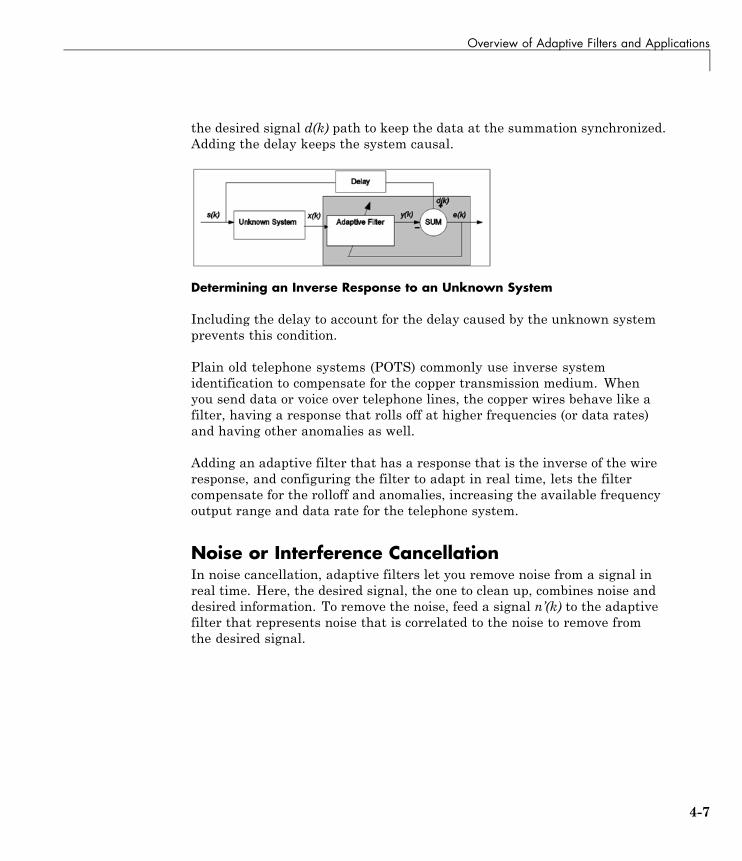
Overview of Adaptive Filters and Applications
the desired signal d(k) path to keep the data at the summation synchronized.Adding the delay keeps the system causal.
Determining an Inverse Response to an Unknown System
Including the delay to account for the delay caused by the unknown systemprevents this condition.
Plain old telephone systems (POTS) commonly use inverse systemidentification to compensate for the copper transmission medium. Whenyou send data or voice over telephone lines, the copper wires behave like afilter, having a response that rolls off at higher frequencies (or data rates)and having other anomalies as well.
Adding an adaptive filter that has a response that is the inverse of the wireresponse, and configuring the filter to adapt in real time, lets the filtercompensate for the rolloff and anomalies, increasing the available frequencyoutput range and data rate for the telephone system.
Noise or Interference CancellationIn noise cancellation, adaptive filters let you remove noise from a signal inreal time. Here, the desired signal, the one to clean up, combines noise anddesired information. To remove the noise, feed a signal n’(k) to the adaptivefilter that represents noise that is correlated to the noise to remove fromthe desired signal.
4-7

4 Adaptive Filters
���� �������� ������
����
���� �����
�
����� ����
����
Using an Adaptive Filter to Remove Noise from an Unknown System
So long as the input noise to the filter remains correlated to the unwantednoise accompanying the desired signal, the adaptive filter adjusts itscoefficients to reduce the value of the difference between y(k) and d(k),removing the noise and resulting in a clean signal in e(k). Notice that inthis application, the error signal actually converges to the input data signal,rather than converging to zero.
PredictionPredicting signals requires that you make some key assumptions. Assumethat the signal is either steady or slowly varying over time, and periodic overtime as well.
���� �������� �������
����
���� �����
�����
���"
Predicting Future Values of a Periodic Signal
Accepting these assumptions, the adaptive filter must predict the futurevalues of the desired signal based on past values. When s(k) is periodic andthe filter is long enough to remember previous values, this structure with thedelay in the input signal, can perform the prediction. You might use thisstructure to remove a periodic signal from stochastic noise signals.
Finally, notice that most systems of interest contain elements of more thanone of the four adaptive filter structures. Carefully reviewing the realstructure may be required to determine what the adaptive filter is adapting to.
4-8

Overview of Adaptive Filters and Applications
Also, for clarity in the figures, the analog-to-digital (A/D) and digital-to-analog(D/A) components do not appear. Since the adaptive filters are assumed to bedigital in nature, and many of the problems produce analog data, convertingthe input signals to and from the analog domain is probably necessary.
4-9

4 Adaptive Filters
Adaptive Filters in DSP System Toolbox Software
In this section...
“Overview of Adaptive Filtering in DSP System Toolbox Software” on page4-10
“Algorithms” on page 4-10
“Using Adaptive Filter Objects” on page 4-13
Overview of Adaptive Filtering in DSP SystemToolbox SoftwareDSP System Toolbox software contains many objects for constructing andapplying adaptive filters to data. As you see in the tables in the next section,the objects use various algorithms to determine the weights for the filtercoefficients of the adapting filter. While the algorithms differ in their detailimplementations, the LMS and RLS share a common operational approach —minimizing the error between the filter output and the desired signal.
AlgorithmsFor adaptive filter (adaptfilt) objects, the algorithm string determineswhich adaptive filter algorithm your adaptfilt object implements. Eachavailable algorithm entry appears in one of the tables along with a briefdescription of the algorithm. Click on the algorithm in the first column to getmore information about the associated adaptive filter technique.
• LMS based adaptive filters
• RLS based adaptive filters
• Affine projection adaptive filters
• Adaptive filters in the frequency domain
• Lattice based adaptive filters
4-10
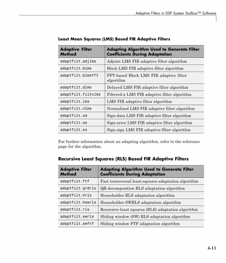
Adaptive Filters in DSP System Toolbox™ Software
Least Mean Squares (LMS) Based FIR Adaptive Filters
Adaptive FilterMethod
Adapting Algorithm Used to Generate FilterCoefficients During Adaptation
adaptfilt.adjlms Adjoint LMS FIR adaptive filter algorithm
adaptfilt.blms Block LMS FIR adaptive filter algorithm
adaptfilt.blmsfft FFT-based Block LMS FIR adaptive filteralgorithm
adaptfilt.dlms Delayed LMS FIR adaptive filter algorithm
adaptfilt.filtxlms Filtered-x LMS FIR adaptive filter algorithm
adaptfilt.lms LMS FIR adaptive filter algorithm
adaptfilt.nlms Normalized LMS FIR adaptive filter algorithm
adaptfilt.sd Sign-data LMS FIR adaptive filter algorithm
adaptfilt.se Sign-error LMS FIR adaptive filter algorithm
adaptfilt.ss Sign-sign LMS FIR adaptive filter algorithm
For further information about an adapting algorithm, refer to the referencepage for the algorithm.
Recursive Least Squares (RLS) Based FIR Adaptive Filters
Adaptive FilterMethod
Adapting Algorithm Used to Generate FilterCoefficients During Adaptation
adaptfilt.ftf Fast transversal least-squares adaptation algorithm
adaptfilt.qrdrls QR-decomposition RLS adaptation algorithm
adaptfilt.hrls Householder RLS adaptation algorithm
adaptfilt.hswrls Householder SWRLS adaptation algorithm
adaptfilt.rls Recursive-least squares (RLS) adaptation algorithm
adaptfilt.swrls Sliding window (SW) RLS adaptation algorithm
adaptfilt.swftf Sliding window FTF adaptation algorithm
4-11

4 Adaptive Filters
For more complete information about an adapting algorithm, refer to thereference page for the algorithm.
Affine Projection (AP) FIR Adaptive Filters
Adaptive FilterMethod
Adapting Algorithm Used to Generate FilterCoefficients During Adaptation
adaptfilt.ap Affine projection algorithm that uses direct matrixinversion
adaptfilt.apru Affine projection algorithm that uses recursive matrixupdating
adaptfilt.bap Block affine projection adaptation algorithm
To find more information about an adapting algorithm, refer to the referencepage for the algorithm.
FIR Adaptive Filters in the Frequency Domain (FD)
Adaptive FilterMethod
Description of the Adapting AlgorithmUsed to Generate Filter Coefficients DuringAdaptation
adaptfilt.fdaf Frequency domain adaptation algorithm
adaptfilt.pbfdaf Partition block version of the FDAF algorithm
adaptfilt.pbufdaf Partition block unconstrained version of the FDAFalgorithm
adaptfilt.tdafdct Transform domain adaptation algorithm usingDCT
adaptfilt.tdafdft Transform domain adaptation algorithm usingDFT
adaptfilt.ufdaf Unconstrained FDAF algorithm for adaptation
For more information about an adapting algorithm, refer to the referencepage for the algorithm.
4-12
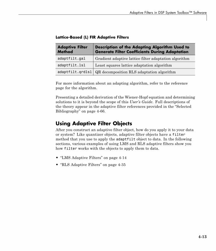
Adaptive Filters in DSP System Toolbox™ Software
Lattice-Based (L) FIR Adaptive Filters
Adaptive FilterMethod
Description of the Adapting Algorithm Used toGenerate Filter Coefficients During Adaptation
adaptfilt.gal Gradient adaptive lattice filter adaptation algorithm
adaptfilt.lsl Least squares lattice adaptation algorithm
adaptfilt.qrdlsl QR decomposition RLS adaptation algorithm
For more information about an adapting algorithm, refer to the referencepage for the algorithm.
Presenting a detailed derivation of the Wiener-Hopf equation and determiningsolutions to it is beyond the scope of this User’s Guide. Full descriptions ofthe theory appear in the adaptive filter references provided in the “SelectedBibliography” on page 4-66.
Using Adaptive Filter ObjectsAfter you construct an adaptive filter object, how do you apply it to your dataor system? Like quantizer objects, adaptive filter objects have a filtermethod that you use to apply the adaptfilt object to data. In the followingsections, various examples of using LMS and RLS adaptive filters show youhow filter works with the objects to apply them to data.
• “LMS Adaptive Filters” on page 4-14
• “RLS Adaptive Filters” on page 4-35
4-13

4 Adaptive Filters
LMS Adaptive Filters
In this section...
“LMS Methods for adaptfilt Objects” on page 4-14
“System Identification Using adaptfilt.lms” on page 4-16
“System Identification Using adaptfilt.nlms” on page 4-19
“Noise Cancellation Using adaptfilt.sd” on page 4-22
“Noise Cancellation Using adaptfilt.se” on page 4-26
“Noise Cancellation Using adaptfilt.ss” on page 4-30
LMS Methods for adaptfilt ObjectsThis section provides introductory examples using some of the least meansquares (LMS) adaptive filter functions in the toolbox.
The toolbox provides many adaptive filter design functions that use the LMSalgorithms to search for the optimal solution to the adaptive filter, including
• adaptfilt.lms— Implement the LMS algorithm to solve the Wiener-Hopfequation and find the filter coefficients for an adaptive filter.
• adaptfilt.nlms — Implement the normalized variation of the LMSalgorithm to solve the Wiener-Hopf equation and determine the filtercoefficients of an adaptive filter.
• adaptfilt.sd— Implement the sign-data variation of the LMS algorithmto solve the Wiener-Hopf equation and determine the filter coefficients ofan adaptive filter. The correction to the filter weights at each iterationdepends on the sign of the input x(k).
• adaptfilt.se— Implement the sign-error variation of the LMS algorithmto solve the Wiener-Hopf equation and determine the filter coefficients ofan adaptive filter. The correction applied to the current filter weights foreach successive iteration depends on the sign of the error, e(k).
• adaptfilt.ss— Implement the sign-sign variation of the LMS algorithmto solve the Wiener-Hopf equation and determine the filter coefficients of an
4-14
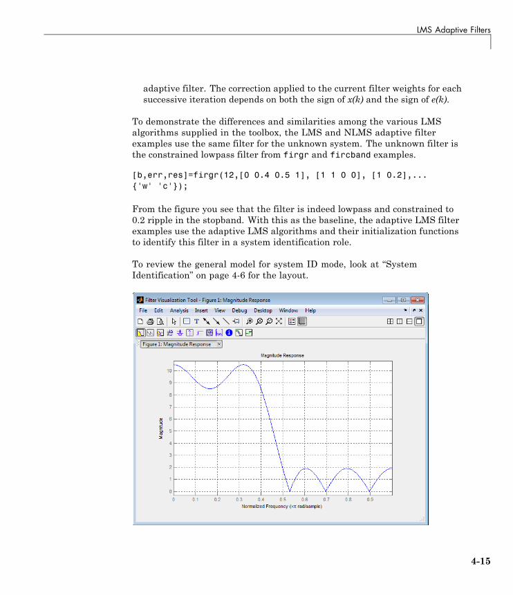
LMS Adaptive Filters
adaptive filter. The correction applied to the current filter weights for eachsuccessive iteration depends on both the sign of x(k) and the sign of e(k).
To demonstrate the differences and similarities among the various LMSalgorithms supplied in the toolbox, the LMS and NLMS adaptive filterexamples use the same filter for the unknown system. The unknown filter isthe constrained lowpass filter from firgr and fircband examples.
[b,err,res]=firgr(12,[0 0.4 0.5 1], [1 1 0 0], [1 0.2],...{'w' 'c'});
From the figure you see that the filter is indeed lowpass and constrained to0.2 ripple in the stopband. With this as the baseline, the adaptive LMS filterexamples use the adaptive LMS algorithms and their initialization functionsto identify this filter in a system identification role.
To review the general model for system ID mode, look at “SystemIdentification” on page 4-6 for the layout.
4-15
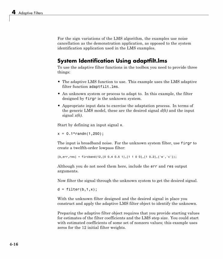
4 Adaptive Filters
For the sign variations of the LMS algorithm, the examples use noisecancellation as the demonstration application, as opposed to the systemidentification application used in the LMS examples.
System Identification Using adaptfilt.lmsTo use the adaptive filter functions in the toolbox you need to provide threethings:
• The adaptive LMS function to use. This example uses the LMS adaptivefilter function adaptfilt.lms.
• An unknown system or process to adapt to. In this example, the filterdesigned by firgr is the unknown system.
• Appropriate input data to exercise the adaptation process. In terms ofthe generic LMS model, these are the desired signal d(k) and the inputsignal x(k).
Start by defining an input signal x.
x = 0.1*randn(1,250);
The input is broadband noise. For the unknown system filter, use firgr tocreate a twelfth-order lowpass filter:
[b,err,res] = fircband(12,[0 0.4 0.5 1],[1 1 0 0],[1 0.2],{'w','c'});
Although you do not need them here, include the err and res outputarguments.
Now filter the signal through the unknown system to get the desired signal.
d = filter(b,1,x);
With the unknown filter designed and the desired signal in place youconstruct and apply the adaptive LMS filter object to identify the unknown.
Preparing the adaptive filter object requires that you provide starting valuesfor estimates of the filter coefficients and the LMS step size. You could startwith estimated coefficients of some set of nonzero values; this example useszeros for the 12 initial filter weights.
4-16

LMS Adaptive Filters
For the step size, 0.8 is a reasonable value — a good compromise betweenbeing large enough to converge well within the 250 iterations (250 inputsample points) and small enough to create an accurate estimate of theunknown filter.
mu = 0.8;ha = adaptfilt.lms(13,mu);
Finally, using the adaptfilt object ha, desired signal, d, and the input to thefilter, x, run the adaptive filter to determine the unknown system and plotthe results, comparing the actual coefficients from firgr to the coefficientsfound by adaptfilt.lms.
[y,e] = filter(ha,x,d);stem([b.' ha.coefficients.'])title('System Identification by Adaptive LMS Algorithm')legend('Actual Filter Weights', 'Estimated Filter Weights',...
'Location', 'NorthEast')
In the stem plot the actual and estimated filter weights are the same. As anexperiment, try changing the step size to 0.2. Repeating the example withmu = 0.2 results in the following stem plot. The estimated weights fail toapproximate the actual weights closely.
4-17

4 Adaptive Filters
Since this may be because you did not iterate over the LMS algorithm enoughtimes, try using 1000 samples. With 1000 samples, the stem plot, shownin the next figure, looks much better, albeit at the expense of much morecomputation. Clearly you should take care to select the step size with both thecomputation required and the fidelity of the estimated filter in mind.
4-18
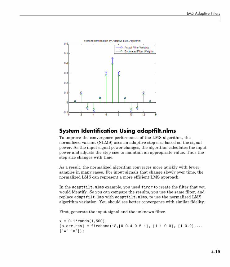
LMS Adaptive Filters
System Identification Using adaptfilt.nlmsTo improve the convergence performance of the LMS algorithm, thenormalized variant (NLMS) uses an adaptive step size based on the signalpower. As the input signal power changes, the algorithm calculates the inputpower and adjusts the step size to maintain an appropriate value. Thus thestep size changes with time.
As a result, the normalized algorithm converges more quickly with fewersamples in many cases. For input signals that change slowly over time, thenormalized LMS can represent a more efficient LMS approach.
In the adaptfilt.nlms example, you used firgr to create the filter that youwould identify. So you can compare the results, you use the same filter, andreplace adaptfilt.lms with adaptfilt.nlms, to use the normalized LMSalgorithm variation. You should see better convergence with similar fidelity.
First, generate the input signal and the unknown filter.
x = 0.1*randn(1,500);[b,err,res] = fircband(12,[0 0.4 0.5 1], [1 1 0 0], [1 0.2],...{'w' 'c'});
4-19
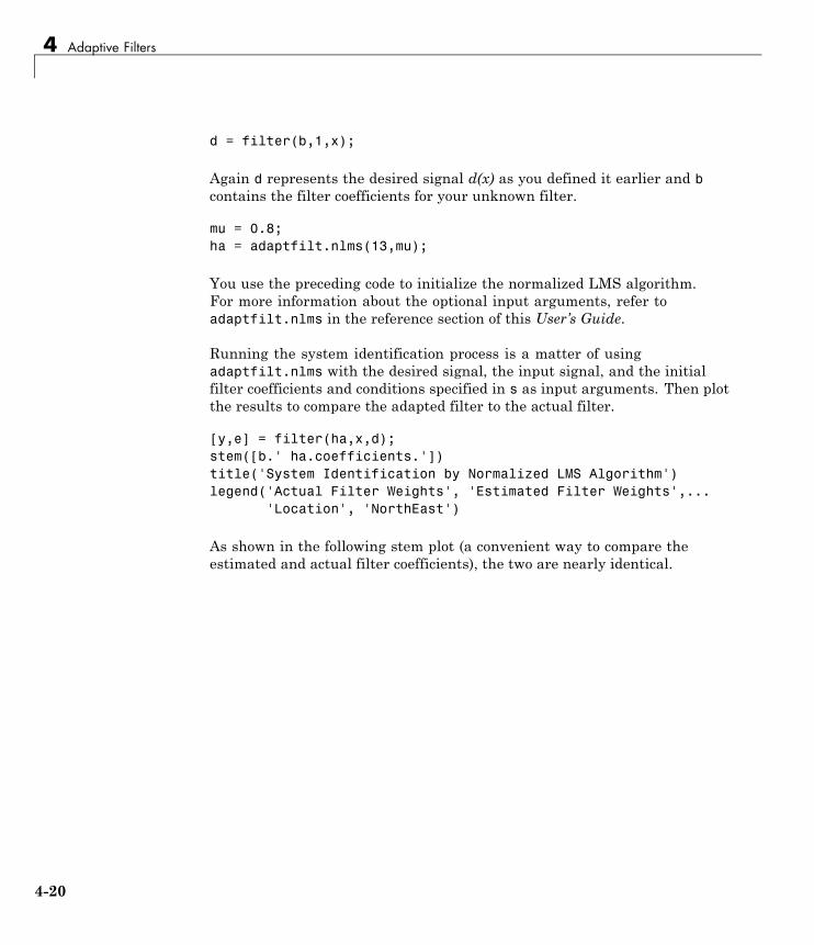
4 Adaptive Filters
d = filter(b,1,x);
Again d represents the desired signal d(x) as you defined it earlier and bcontains the filter coefficients for your unknown filter.
mu = 0.8;ha = adaptfilt.nlms(13,mu);
You use the preceding code to initialize the normalized LMS algorithm.For more information about the optional input arguments, refer toadaptfilt.nlms in the reference section of this User’s Guide.
Running the system identification process is a matter of usingadaptfilt.nlms with the desired signal, the input signal, and the initialfilter coefficients and conditions specified in s as input arguments. Then plotthe results to compare the adapted filter to the actual filter.
[y,e] = filter(ha,x,d);stem([b.' ha.coefficients.'])title('System Identification by Normalized LMS Algorithm')legend('Actual Filter Weights', 'Estimated Filter Weights',...
'Location', 'NorthEast')
As shown in the following stem plot (a convenient way to compare theestimated and actual filter coefficients), the two are nearly identical.
4-20
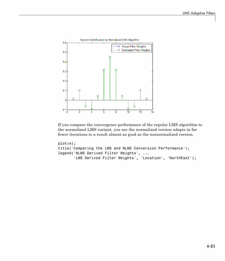
LMS Adaptive Filters
If you compare the convergence performance of the regular LMS algorithm tothe normalized LMS variant, you see the normalized version adapts in farfewer iterations to a result almost as good as the nonnormalized version.
plot(e);title('Comparing the LMS and NLMS Conversion Performance');legend('NLMS Derived Filter Weights', ...
'LMS Derived Filter Weights', 'Location', 'NorthEast');
4-21
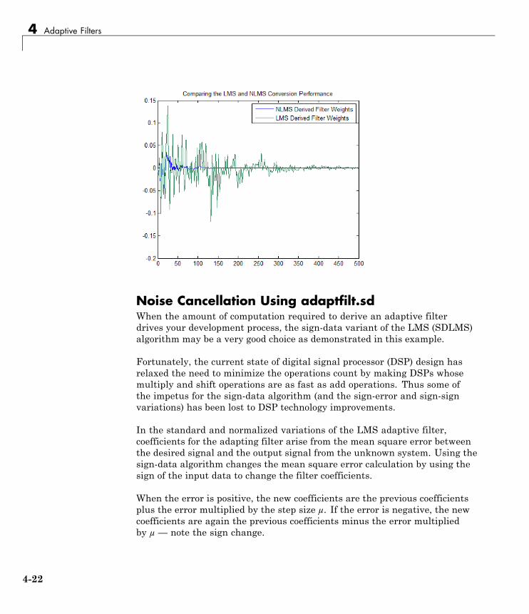
4 Adaptive Filters
Noise Cancellation Using adaptfilt.sdWhen the amount of computation required to derive an adaptive filterdrives your development process, the sign-data variant of the LMS (SDLMS)algorithm may be a very good choice as demonstrated in this example.
Fortunately, the current state of digital signal processor (DSP) design hasrelaxed the need to minimize the operations count by making DSPs whosemultiply and shift operations are as fast as add operations. Thus some ofthe impetus for the sign-data algorithm (and the sign-error and sign-signvariations) has been lost to DSP technology improvements.
In the standard and normalized variations of the LMS adaptive filter,coefficients for the adapting filter arise from the mean square error betweenthe desired signal and the output signal from the unknown system. Using thesign-data algorithm changes the mean square error calculation by using thesign of the input data to change the filter coefficients.
When the error is positive, the new coefficients are the previous coefficientsplus the error multiplied by the step size µ. If the error is negative, the newcoefficients are again the previous coefficients minus the error multipliedby µ — note the sign change.
4-22

LMS Adaptive Filters
When the input is zero, the new coefficients are the same as the previous set.
In vector form, the sign-data LMS algorithm is
w k w k e k x k
x kx kx kx
( ) ( ) ( )sgn ( ) ,
sgn ( ), ( ), ( ), (
+ = + [ ]
[ ] =>=
−
1
1 00 0
1
kk) <
⎧⎨⎪
⎩⎪ 0
with vector w containing the weights applied to the filter coefficients andvector x containing the input data. e(k) (equal to desired signal - filteredsignal) is the error at time k and is the quantity the SDLMS algorithm seeksto minimize. µ (mu) is the step size.
As you specify mu smaller, the correction to the filter weights gets smallerfor each sample and the SDLMS error falls more slowly. Larger mu changesthe weights more for each step so the error falls more rapidly, but theresulting error does not approach the ideal solution as closely. To ensure goodconvergence rate and stability, select mu within the following practical bounds
01< < { }
N InputSignalPower
where N is the number of samples in the signal. Also, define mu as a power oftwo for efficient computing.
Note How you set the initial conditions of the sign-data algorithm profoundlyinfluences the effectiveness of the adaptation. Because the algorithmessentially quantizes the input signal, the algorithm can become unstableeasily.
A series of large input values, coupled with the quantization process mayresult in the error growing beyond all bounds. You restrain the tendency ofthe sign-data algorithm to get out of control by choosing a small step size (µ<<1) and setting the initial conditions for the algorithm to nonzero positiveand negative values.
4-23
4 Adaptive Filters
In this noise cancellation example, adaptfilt.sd requires two input datasets:
• Data containing a signal corrupted by noise. In Using an Adaptive Filterto Remove Noise from an Unknown System on page 4-8, this is d(k), thedesired signal. The noise cancellation process removes the noise, leavingthe signal.
• Data containing random noise (x(k) in Using an Adaptive Filter to RemoveNoise from an Unknown System on page 4-8) that is correlated with thenoise that corrupts the signal data. Without the correlation between thenoise data, the adapting algorithm cannot remove the noise from the signal.
For the signal, use a sine wave. Note that signal is a column vector of 1000elements.
signal = sin(2*pi*0.055*[0:1000-1]');
Now, add correlated white noise to signal. To ensure that the noise iscorrelated, pass the noise through a lowpass FIR filter, and then add thefiltered noise to the signal.
noise=randn(1,1000);nfilt=fir1(11,0.4); % Eleventh order lowpass filterfnoise=filter(nfilt,1,noise); % Correlated noise datad=signal.'+fnoise;
fnoise is the correlated noise and d is now the desired input to the sign-dataalgorithm.
To prepare the adaptfilt object for processing, set the input conditionscoeffs and mu for the object. As noted earlier in this section, the values youset for coeffs and mu determine whether the adaptive filter can remove thenoise from the signal path.
In “System Identification Using adaptfilt.lms” on page 4-16, you constructeda default filter that sets the filter coefficients to zeros. In most cases thatapproach does not work for the sign-data algorithm. The closer you set yourinitial filter coefficients to the expected values, the more likely it is thatthe algorithm remains well behaved and converges to a filter solution thatremoves the noise effectively.
4-24

LMS Adaptive Filters
For this example, start with the coefficients in the filter you used to filter thenoise (nfilt), and modify them slightly so the algorithm has to adapt.
coeffs = nfilt.' -0.01; % Set the filter initial conditions.mu = 0.05; % Set the step size for algorithm updating.
With the required input arguments for adaptfilt.sd prepared, construct theadaptfilt object, run the adaptation, and view the results.
ha = adaptfilt.sd(12,mu)set(ha,'coefficients',coeffs);[y,e] = filter(ha,noise,d);plot(0:199,signal(1:200),0:199,e(1:200));title('Noise Cancellation by the Sign-Data Algorithm');legend('Actual Signal', 'Result of Noise Cancellation',...
'Location', 'NorthEast');
When adaptfilt.sd runs, it uses far fewer multiply operations than either ofthe LMS algorithms. Also, performing the sign-data adaptation requires onlybit shifting multiplies when the step size is a power of two.
Although the performance of the sign-data algorithm as shown in the nextfigure is quite good, the sign-data algorithm is much less stable than thestandard LMS variations. In this noise cancellation example, the signal afterprocessing is a very good match to the input signal, but the algorithm couldvery easily grow without bound rather than achieve good performance.
Changing coeffs, mu, or even the lowpass filter you used to create thecorrelated noise can cause noise cancellation to fail and the algorithm tobecome useless.
4-25
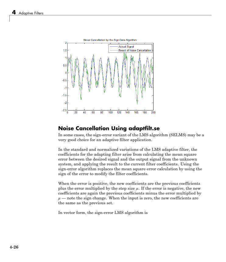
4 Adaptive Filters
Noise Cancellation Using adaptfilt.seIn some cases, the sign-error variant of the LMS algorithm (SELMS) may be avery good choice for an adaptive filter application.
In the standard and normalized variations of the LMS adaptive filter, thecoefficients for the adapting filter arise from calculating the mean squareerror between the desired signal and the output signal from the unknownsystem, and applying the result to the current filter coefficients. Using thesign-error algorithm replaces the mean square error calculation by using thesign of the error to modify the filter coefficients.
When the error is positive, the new coefficients are the previous coefficientsplus the error multiplied by the step size µ. If the error is negative, the newcoefficients are again the previous coefficients minus the error multiplied byµ — note the sign change. When the input is zero, the new coefficients arethe same as the previous set.
In vector form, the sign-error LMS algorithm is
4-26

LMS Adaptive Filters
w k w k e k x k
e ke ke k
( ) ( ) sgn ( ) ( ) ,
sgn ( ), ( ), ( ),
+ = + [ ][ ]
[ ] =>=
−
1
1 00 0
1
ee k( ) <
⎧⎨⎪
⎩⎪
⎫⎬⎪
⎭⎪0
with vector w containing the weights applied to the filter coefficients andvector x containing the input data. e(k) (equal to desired signal - filteredsignal) is the error at time k and is the quantity the SELMS algorithm seeksto minimize. µ (mu) is the step size. As you specify mu smaller, the correctionto the filter weights gets smaller for each sample and the SELMS error fallsmore slowly.
Larger mu changes the weights more for each step so the error falls morerapidly, but the resulting error does not approach the ideal solution as closely.To ensure good convergence rate and stability, select mu within the followingpractical bounds
01< < { }
N InputSignalPower
where N is the number of samples in the signal. Also, define mu as a power oftwo for efficient computation.
Note How you set the initial conditions of the sign-data algorithm profoundlyinfluences the effectiveness of the adaptation. Because the algorithmessentially quantizes the error signal, the algorithm can become unstableeasily.
A series of large error values, coupled with the quantization process mayresult in the error growing beyond all bounds. You restrain the tendency ofthe sign-error algorithm to get out of control by choosing a small step size(µ<< 1) and setting the initial conditions for the algorithm to nonzero positiveand negative values.
In this noise cancellation example, adaptfilt.se requires two input datasets:
4-27
4 Adaptive Filters
• Data containing a signal corrupted by noise. In Using an Adaptive Filterto Remove Noise from an Unknown System on page 4-8, this is d(k), thedesired signal. The noise cancellation process removes the noise, leavingthe signal.
• Data containing random noise (x(k) in Using an Adaptive Filter to RemoveNoise from an Unknown System on page 4-8) that is correlated with thenoise that corrupts the signal data. Without the correlation between thenoise data, the adapting algorithm cannot remove the noise from the signal.
For the signal, use a sine wave. Note that signal is a column vector of 1000elements.
signal = sin(2*pi*0.055*[0:1000-1]');
Now, add correlated white noise to signal. To ensure that the noise iscorrelated, pass the noise through a lowpass FIR filter, then add the filterednoise to the signal.
noise=randn(1,1000);nfilt=fir1(11,0.4); % Eleventh order lowpass filter.fnoise=filter(nfilt,1,noise); % Correlated noise data.d=signal.'+fnoise;
fnoise is the correlated noise and d is now the desired input to the sign-dataalgorithm.
To prepare the adaptfilt object for processing, set the input conditionscoeffs and mu for the object. As noted earlier in this section, the values youset for coeffs and mu determine whether the adaptive filter can remove thenoise from the signal path. In “System Identification Using adaptfilt.lms”on page 4-16, you constructed a default filter that sets the filter coefficientsto zeros.
Setting the coefficients to zero often does not work for the sign-erroralgorithm. The closer you set your initial filter coefficients to the expectedvalues, the more likely it is that the algorithm remains well behaved andconverges to a filter solution that removes the noise effectively.
For this example, you start with the coefficients in the filter you used to filterthe noise (nfilt), and modify them slightly so the algorithm has to adapt.
4-28
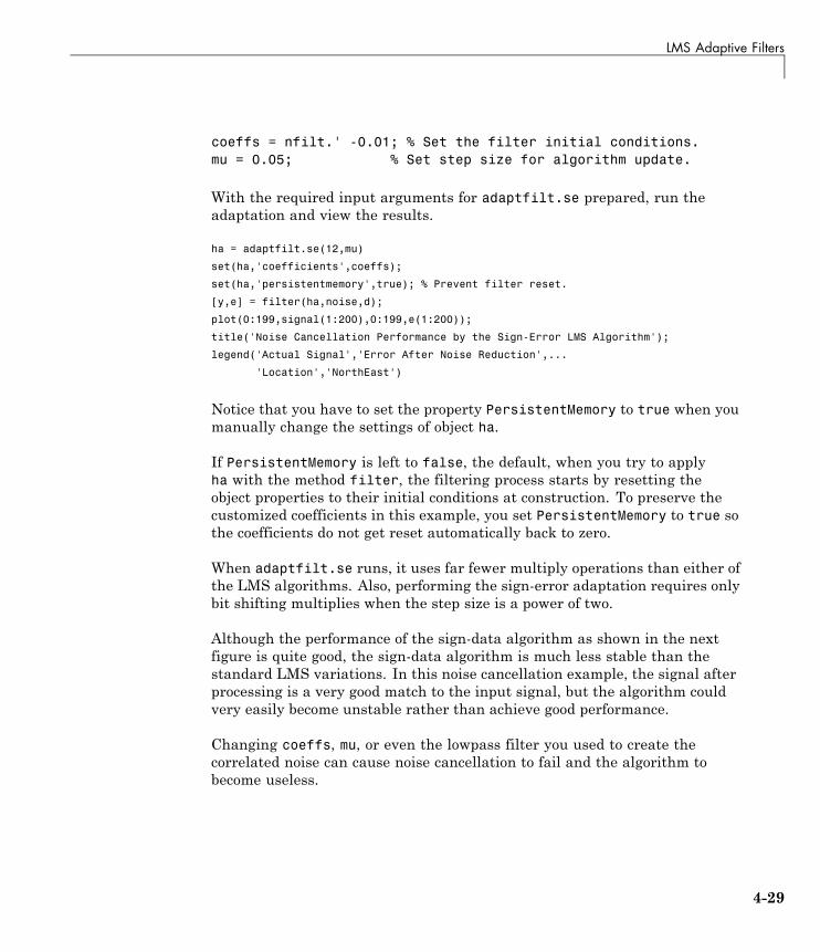
LMS Adaptive Filters
coeffs = nfilt.' -0.01; % Set the filter initial conditions.mu = 0.05; % Set step size for algorithm update.
With the required input arguments for adaptfilt.se prepared, run theadaptation and view the results.
ha = adaptfilt.se(12,mu)
set(ha,'coefficients',coeffs);
set(ha,'persistentmemory',true); % Prevent filter reset.
[y,e] = filter(ha,noise,d);
plot(0:199,signal(1:200),0:199,e(1:200));
title('Noise Cancellation Performance by the Sign-Error LMS Algorithm');
legend('Actual Signal','Error After Noise Reduction',...
'Location','NorthEast')
Notice that you have to set the property PersistentMemory to true when youmanually change the settings of object ha.
If PersistentMemory is left to false, the default, when you try to applyha with the method filter, the filtering process starts by resetting theobject properties to their initial conditions at construction. To preserve thecustomized coefficients in this example, you set PersistentMemory to true sothe coefficients do not get reset automatically back to zero.
When adaptfilt.se runs, it uses far fewer multiply operations than either ofthe LMS algorithms. Also, performing the sign-error adaptation requires onlybit shifting multiplies when the step size is a power of two.
Although the performance of the sign-data algorithm as shown in the nextfigure is quite good, the sign-data algorithm is much less stable than thestandard LMS variations. In this noise cancellation example, the signal afterprocessing is a very good match to the input signal, but the algorithm couldvery easily become unstable rather than achieve good performance.
Changing coeffs, mu, or even the lowpass filter you used to create thecorrelated noise can cause noise cancellation to fail and the algorithm tobecome useless.
4-29
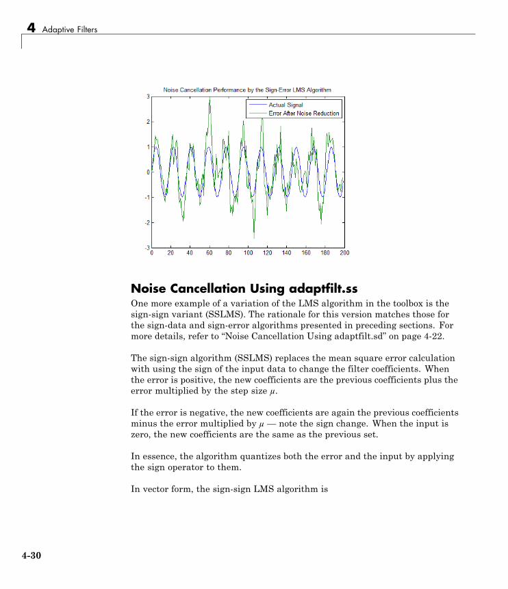
4 Adaptive Filters
Noise Cancellation Using adaptfilt.ssOne more example of a variation of the LMS algorithm in the toolbox is thesign-sign variant (SSLMS). The rationale for this version matches those forthe sign-data and sign-error algorithms presented in preceding sections. Formore details, refer to “Noise Cancellation Using adaptfilt.sd” on page 4-22.
The sign-sign algorithm (SSLMS) replaces the mean square error calculationwith using the sign of the input data to change the filter coefficients. Whenthe error is positive, the new coefficients are the previous coefficients plus theerror multiplied by the step size µ.
If the error is negative, the new coefficients are again the previous coefficientsminus the error multiplied by µ — note the sign change. When the input iszero, the new coefficients are the same as the previous set.
In essence, the algorithm quantizes both the error and the input by applyingthe sign operator to them.
In vector form, the sign-sign LMS algorithm is
4-30

LMS Adaptive Filters
w k w k e k x k
z kz kz k
( ) ( ) sgn ( ) sgn ( ) ,
sgn ( ), ( ), ( )
+ = + [ ] [ ]
[ ] =>=
1
1 00 0
−− <
⎧⎨⎪
⎩⎪ 1 0, ( )z k
where
z k e k x k( ) ( ) sgn ( )= [ ] [ ]
Vector w contains the weights applied to the filter coefficients and vector xcontains the input data. e(k) ( = desired signal - filtered signal) is the error attime k and is the quantity the SSLMS algorithm seeks to minimize. µ(mu) isthe step size. As you specify mu smaller, the correction to the filter weightsgets smaller for each sample and the SSLMS error falls more slowly.
Larger mu changes the weights more for each step so the error falls morerapidly, but the resulting error does not approach the ideal solution as closely.To ensure good convergence rate and stability, select mu within the followingpractical bounds
01< < { }
N InputSignalPower
where N is the number of samples in the signal. Also, define mu as a power oftwo for efficient computation.
4-31

4 Adaptive Filters
Note How you set the initial conditions of the sign-sign algorithm profoundlyinfluences the effectiveness of the adaptation. Because the algorithmessentially quantizes the input signal and the error signal, the algorithmcan become unstable easily.
A series of large error values, coupled with the quantization process mayresult in the error growing beyond all bounds. You restrain the tendency ofthe sign-sign algorithm to get out of control by choosing a small step size (µ<<1) and setting the initial conditions for the algorithm to nonzero positiveand negative values.
In this noise cancellation example, adaptfilt.ss requires two input datasets:
• Data containing a signal corrupted by noise. In Using an Adaptive Filterto Remove Noise from an Unknown System on page 4-8, this is d(k), thedesired signal. The noise cancellation process removes the noise, leavingthe cleaned signal as the content of the error signal.
• Data containing random noise (x(k) in Using an Adaptive Filter to RemoveNoise from an Unknown System on page 4-8) that is correlated with thenoise that corrupts the signal data, called. Without the correlation betweenthe noise data, the adapting algorithm cannot remove the noise from thesignal.
For the signal, use a sine wave. Note that signal is a column vector of 1000elements.
signal = sin(2*pi*0.055*[0:1000-1]');
Now, add correlated white noise to signal. To ensure that the noise iscorrelated, pass the noise through a lowpass FIR filter, then add the filterednoise to the signal.
noise=randn(1,1000);nfilt=fir1(11,0.4); % Eleventh order lowpass filterfnoise=filter(nfilt,1,noise); % Correlated noise datad=signal.'+fnoise;
4-32
LMS Adaptive Filters
fnoise is the correlated noise and d is now the desired input to the sign-dataalgorithm.
To prepare the adaptfilt object for processing, set the input conditionscoeffs and mu for the object. As noted earlier in this section, the values youset for coeffs and mu determine whether the adaptive filter can remove thenoise from the signal path. In “System Identification Using adaptfilt.lms” onpage 4-16, you constructed a default filter that sets the filter coefficients tozeros. Usually that approach does not work for the sign-sign algorithm.
The closer you set your initial filter coefficients to the expected values, themore likely it is that the algorithm remains well behaved and converges to afilter solution that removes the noise effectively. For this example, you startwith the coefficients in the filter you used to filter the noise (nfilt), andmodify them slightly so the algorithm has to adapt.
coeffs = nfilt.' -0.01; % Set the filter initial conditions.mu = 0.05; % Set the step size for algorithm updating.
With the required input arguments for adaptfilt.ss prepared, run theadaptation and view the results.
ha = adaptfilt.ss(12,mu)
set(ha,'coefficients',coeffs);
set(ha,'persistentmemory',true); % Prevent filter reset.
[y,e] = filter(ha,noise,d);
plot(0:199,signal(1:200),0:199,e(1:200));
title('Noise Cancellation Performance of the Sign-Sign LMS Algorithm');
legend('Actual Signal', 'Error After Noise Reduction', ...
'Location', 'NorthEast');
Notice that you have to set the property PersistentMemory to true when youmanually change the settings of object ha.
If PersistentMemory is left to false, when you try to apply ha with themethod filter the filtering process starts by resetting the object properties totheir initial conditions at construction. To preserve the customized coefficientsin this example, you set PersistentMemory to true so the coefficients do notget reset automatically back to zero.
4-33

4 Adaptive Filters
When adaptfilt.ss runs, it uses far fewer multiply operations than either ofthe LMS algorithms. Also, performing the sign-sign adaptation requires onlybit shifting multiplies when the step size is a power of two.
Although the performance of the sign-sign algorithm as shown in the nextfigure is quite good, the sign-sign algorithm is much less stable than thestandard LMS variations. In this noise cancellation example, the signal afterprocessing is a very good match to the input signal, but the algorithm couldvery easily become unstable rather than achieve good performance.
Changing coeffs, mu, or even the lowpass filter you used to create thecorrelated noise can cause noise cancellation to fail and the algorithm tobecome useless.
As an aside, the sign-sign LMS algorithm is part of the international CCITTstandard for 32 Kb/s ADPCM telephony.
4-34
RLS Adaptive Filters
RLS Adaptive Filters
In this section...
“Compare RLS and LMS Adaptive Filter Algorithms” on page 4-35
“Inverse System Identification Using adaptfilt.rls” on page 4-36
Compare RLS and LMS Adaptive Filter AlgorithmsThis section provides an introductory example that uses the RLS adaptivefilter function adaptfilt.rls.
If LMS algorithms represent the simplest and most easily applied adaptivealgorithms, the recursive least squares (RLS) algorithms represents increasedcomplexity, computational cost, and fidelity. In performance, RLS approachesthe Kalman filter in adaptive filtering applications, at somewhat reducedrequired throughput in the signal processor.
Compared to the LMS algorithm, the RLS approach offers faster convergenceand smaller error with respect to the unknown system, at the expense ofrequiring more computations.
In contrast to the least mean squares algorithm, from which it can be derived,the RLS adaptive algorithm minimizes the total squared error between thedesired signal and the output from the unknown system.
Note that the signal paths and identifications are the same whether the filteruses RLS or LMS. The difference lies in the adapting portion.
Within limits, you can use any of the adaptive filter algorithms to solve anadaptive filter problem by replacing the adaptive portion of the applicationwith a new algorithm.
Examples of the sign variants of the LMS algorithms demonstrated thisfeature to demonstrate the differences between the sign-data, sign-error, andsign-sign variations of the LMS algorithm.
4-35
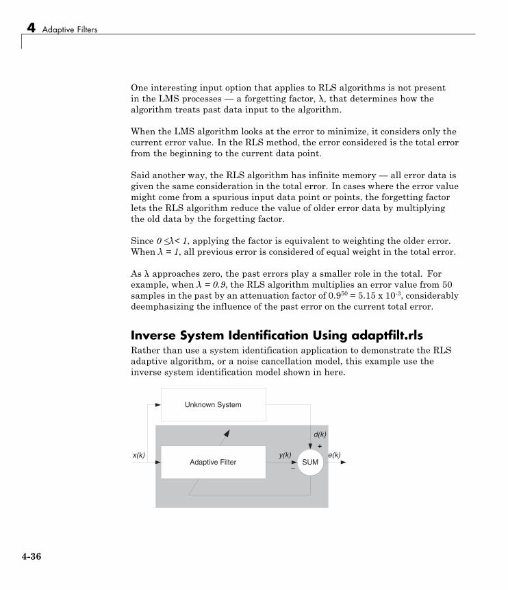
4 Adaptive Filters
One interesting input option that applies to RLS algorithms is not presentin the LMS processes — a forgetting factor, λ, that determines how thealgorithm treats past data input to the algorithm.
When the LMS algorithm looks at the error to minimize, it considers only thecurrent error value. In the RLS method, the error considered is the total errorfrom the beginning to the current data point.
Said another way, the RLS algorithm has infinite memory — all error data isgiven the same consideration in the total error. In cases where the error valuemight come from a spurious input data point or points, the forgetting factorlets the RLS algorithm reduce the value of older error data by multiplyingthe old data by the forgetting factor.
Since 0 ≤λ< 1, applying the factor is equivalent to weighting the older error.When λ = 1, all previous error is considered of equal weight in the total error.
As λ approaches zero, the past errors play a smaller role in the total. Forexample, when λ = 0.9, the RLS algorithm multiplies an error value from 50samples in the past by an attenuation factor of 0.950 = 5.15 x 10⁻³, considerablydeemphasizing the influence of the past error on the current total error.
Inverse System Identification Using adaptfilt.rlsRather than use a system identification application to demonstrate the RLSadaptive algorithm, or a noise cancellation model, this example use theinverse system identification model shown in here.
����
�� ��!���"����
���� �������� �������
����
���� �����
�
4-36

RLS Adaptive Filters
Cascading the adaptive filter with the unknown filter causes the adaptivefilter to converge to a solution that is the inverse of the unknown system.
If the transfer function of the unknown is H(z) and the adaptive filtertransfer function is G(z), the error measured between the desired signaland the signal from the cascaded system reaches its minimum when theproduct of H(z) and G(z) is 1, G(z)*H(z) = 1. For this relation to be true,G(z) must equal 1/H(z), the inverse of the transfer function of the unknownsystem.
To demonstrate that this is true, create a signal to input to the cascadedfilter pair.
x = randn(1,3000);
In the cascaded filters case, the unknown filter results in a delay in the signalarriving at the summation point after both filters. To prevent the adaptivefilter from trying to adapt to a signal it has not yet seen (equivalent topredicting the future), delay the desired signal by 32 samples, the order ofthe unknown system.
Generally, you do not know the order of the system you are trying to identify.In that case, delay the desired signal by the number of samples equal to halfthe order of the adaptive filter. Delaying the input requires prepending 12zero-values samples to x.
delay = zeros(1,12);d = [delay x(1:2988)]; % Concatenate the delay and the signal.
You have to keep the desired signal vector d the same length as x, henceadjust the signal element count to allow for the delay samples.
Although not generally true, for this example you know the order of theunknown filter, so you add a delay equal to the order of the unknown filter.
For the unknown system, use a lowpass, 12th-order FIR filter.
ufilt = fir1(12,0.55,'low');
Filtering x provides the input data signal for the adaptive algorithm function.
4-37

4 Adaptive Filters
xdata = filter(ufilt,1,x);
To set the input argument values for the adaptfilt.rls object, use theconstructor adaptfilt.rls, providing the needed arguments l, lambda, andinvcov.
For more information about the input conditions to prepare the RLS algorithmobject, refer to adaptfilt.rls in the reference section of this user’s guide.
p0 = 2*eye(13);lambda = 0.99;ha = adaptfilt.rls(13,lambda,p0);
Most of the process to this point is the same as the preceding examples.However, since this example seeks to develop an inverse solution, you need tobe careful about which signal carries the data and which is the desired signal.
Earlier examples of adaptive filters use the filtered noise as the desiredsignal. In this case, the filtered noise (xdata) carries the unknown systeminformation. With Gaussian distribution and variance of 1, the unfilterednoise d is the desired signal. The code to run this adaptive filter example is
[y,e] = filter(ha,xdata,d);
where y returns the coefficients of the adapted filter and e contains the errorsignal as the filter adapts to find the inverse of the unknown system. You canreview the returned elements of the adapted filter in the properties of ha.
The next figure presents the results of the adaptation. In the figure, themagnitude response curves for the unknown and adapted filters show. As areminder, the unknown filter was a lowpass filter with cutoff at 0.55, on thenormalized frequency scale from 0 to 1.
4-38

RLS Adaptive Filters
0 0.1 0.2 0.3 0.4 0.5 0.6 0.7 0.8 0.9 1−1200
−1000
−800
−600
−400
−200
0
Normalized Frequency (×π rad/sample)
Pha
se (
degr
ees)
0 0.1 0.2 0.3 0.4 0.5 0.6 0.7 0.8 0.9 1−150
−100
−50
0
50
Normalized Frequency (×π rad/sample)
Mag
nitu
de (
dB)
Comparing the Inverse Filter to the Unknown System
Inverse FilterUnknown System
Viewed alone (refer to the following figure), the inverse system looks like afair compensator for the unknown lowpass filter — a high pass filter withlinear phase.
4-39
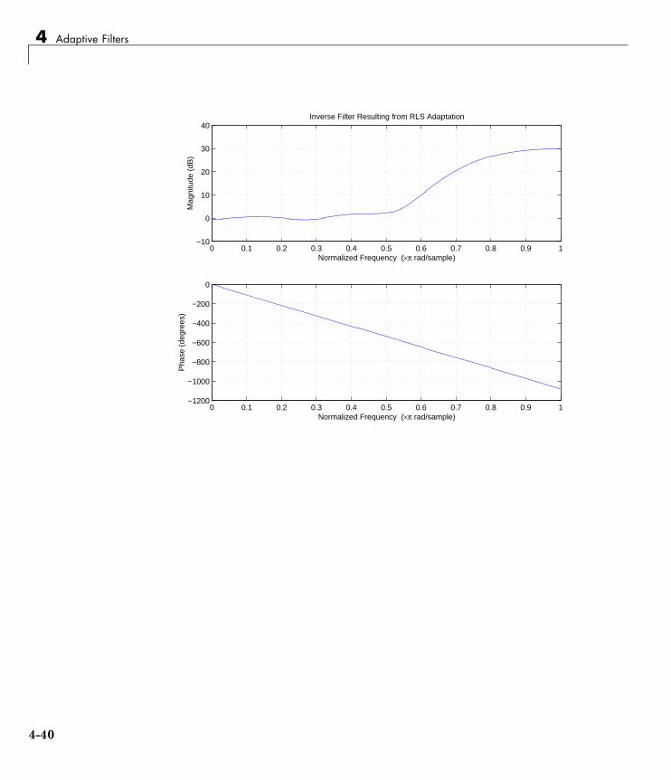
4 Adaptive Filters
0 0.1 0.2 0.3 0.4 0.5 0.6 0.7 0.8 0.9 1−1200
−1000
−800
−600
−400
−200
0
Normalized Frequency (×π rad/sample)
Pha
se (
degr
ees)
0 0.1 0.2 0.3 0.4 0.5 0.6 0.7 0.8 0.9 1−10
0
10
20
30
40
Normalized Frequency (×π rad/sample)
Mag
nitu
de (
dB)
Inverse Filter Resulting from RLS Adaptation
4-40

Signal Enhancement Using LMS and Normalized LMS
Signal Enhancement Using LMS and Normalized LMS
In this section...
“Create the Signals for Adaptation” on page 4-41
“Construct Two Adaptive Filters” on page 4-42
“Choose the Step Size” on page 4-43
“Set the Adapting Filter Step Size” on page 4-44
“Filter with the Adaptive Filters” on page 4-44
“Compute the Optimal Solution” on page 4-44
“Plot the Results” on page 4-45
“Compare the Final Coefficients” on page 4-46
“Reset the Filter Before Filtering” on page 4-47
“Investigate Convergence Through Learning Curves” on page 4-47
“Compute the Learning Curves” on page 4-48
“Compute the Theoretical Learning Curves” on page 4-49
This example illustrates one way to use a few of the adaptive filter algorithmsprovided in the toolbox. In this example, a signal enhancement applicationis used as an illustration. While there are about 30 different adaptivefiltering algorithms included with the toolbox, this example demonstratestwo algorithms — least means square (LMS), using adaptfilt.lms, andnormalized LMS, using adaptfilt.nlms, for adaptation.
Create the Signals for AdaptationThe goal is to use an adaptive filter to extract a desired signal from anoise-corrupted signal by filtering out the noise. The desired signal (theoutput from the process) is a sinusoid with 1000 samples.
n = (1:1000)';s = sin(0.075*pi*n);
To perform adaptation requires two signals:
4-41
4 Adaptive Filters
• a reference signal
• a noisy signal that contains both the desired signal and an added noisecomponent.
Generate the Noise SignalTo create a noise signal, assume that the noise v1 is autoregressive, meaningthat the value of the noise at time t depends only on its previous values andon a random disturbance.
v = 0.8*randn(1000,1); % Random noise part.ar = [1,1/2]; % Autoregression coefficients.v1 = filter(1,ar,v); % Noise signal. Applies a 1-D digital
% filter.
Corrupt the Desired Signal to Create a Noisy SignalTo generate the noisy signal that contains both the desired signal and thenoise, add the noise signal v1 to the desired signal s. The noise-corruptedsinusoid x is
x = s + v1;
where s is the desired signal and the noise is v1. Adaptive filter processingseeks to recover s from x by removing v1. To complete the signals needed toperform adaptive filtering, the adaptation process requires a reference signal.
Create a Reference SignalDefine a moving average signal v2 that is correlated with v1. This v2 is thereference signal for the examples.
ma = [1, -0.8, 0.4 , -0.2];v2 = filter(ma,1,v);
Construct Two Adaptive FiltersTwo similar adaptive filters — LMS and NLMS — form the basis of thisexample, both sixth order. Set the order as a variable in MATLAB and createthe filters.
L = 7;
4-42
Signal Enhancement Using LMS and Normalized LMS
hlms = adaptfilt.lms(7);
hnlms = adaptfilt.nlms(7);
Choose the Step SizeLMS-like algorithms have a step size that determines the amount ofcorrection applied as the filter adapts from one iteration to the next. Choosingthe appropriate step size is not always easy, usually requiring experience inadaptive filter design.
• A step size that is too small increases the time for the filter to converge ona set of coefficients. This becomes an issue of speed and accuracy.
• One that is too large may cause the adapting filter to diverge, neverreaching convergence. In this case, the issue is stability — the resultingfilter might not be stable.
As a rule of thumb, smaller step sizes improve the accuracy of the convergenceof the filter to match the characteristics of the unknown, at the expense of thetime it takes to adapt.
The toolbox includes an algorithm — maxstep— to determine the maximumstep size suitable for each LMS adaptive filter algorithm that still ensuresthat the filter converges to a solution. Often, the notation for the step size is µ.
>> [mumaxlms,mumaxmselms] = maxstep(hlms,x)[mumaxnlms,mumaxmsenlms] = maxstep(hnlms);Warning: Step size is not in the range 0 < mu < mumaxmse/2:Erratic behavior might result.> In adaptfilt.lms.maxstep at 32
mumaxlms =
0.2096
mumaxmselms =
0.1261
4-43

4 Adaptive Filters
Set the Adapting Filter Step SizeThe first output of maxstep is the value needed for the mean of the coefficientsto converge while the second is the value needed for the mean squaredcoefficients to converge. Choosing a large step size often causes largevariations from the convergence values, so choose smaller step sizes generally.
hlms.StepSize = mumaxmselms/30;% This can also be set graphically: inspect(hlms)hnlms.StepSize = mumaxmsenlms/20;% This can also be set graphically: inspect(hnlms)
If you know the step size to use, you can set the step size value with the stepinput argument when you create your filter.
hlms = adaptfilt.lms(N,step); Adds the step input argument.
Filter with the Adaptive FiltersNow you have set up the parameters of the adaptive filters and you are readyto filter the noisy signal. The reference signal, v2, is the input to the adaptivefilters. x is the desired signal in this configuration.
Through adaptation, y, the output of the filters, tries to emulate x as closelyas possible.
Since v2 is correlated only with the noise component v1 of x, it can onlyreally emulate v1. The error signal (the desired x), minus the actual outputy, constitutes an estimate of the part of x that is not correlated with v2— s,the signal to extract from x.
[ylms,elms] = filter(hlms,v2,x);[ynlms,enlms] = filter(hnlms,v2,x);
Compute the Optimal SolutionFor comparison, compute the optimal FIR Wiener filter.
bw = firwiener(L-1,v2,x); % Optimal FIR Wiener filteryw = filter(bw,1,v2); % Estimate of x using Wiener filterew = x - yw; % Estimate of actual sinusoid
4-44
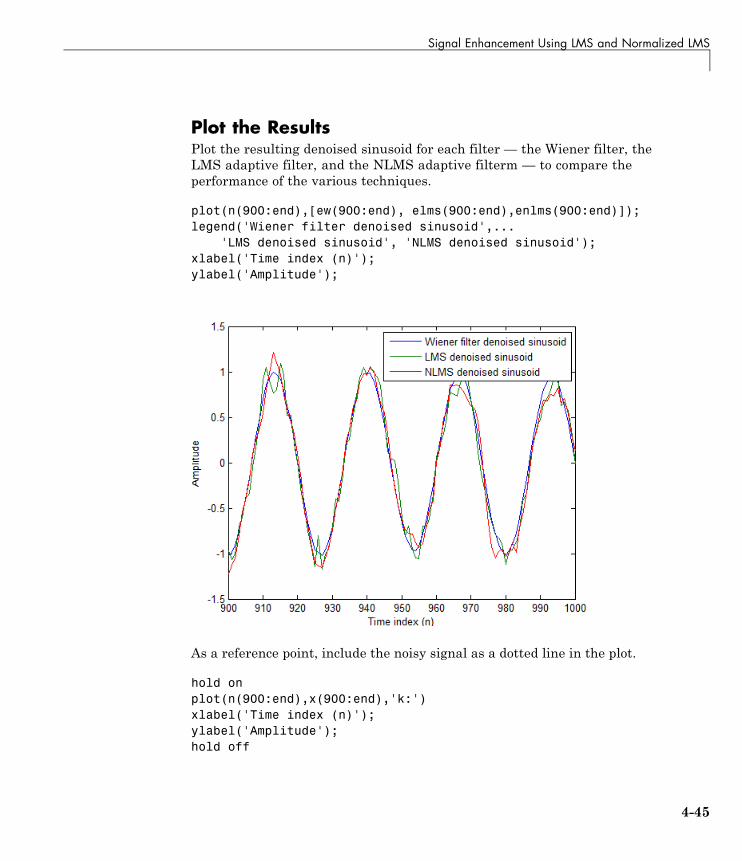
Signal Enhancement Using LMS and Normalized LMS
Plot the ResultsPlot the resulting denoised sinusoid for each filter — the Wiener filter, theLMS adaptive filter, and the NLMS adaptive filterm — to compare theperformance of the various techniques.
plot(n(900:end),[ew(900:end), elms(900:end),enlms(900:end)]);legend('Wiener filter denoised sinusoid',...
'LMS denoised sinusoid', 'NLMS denoised sinusoid');xlabel('Time index (n)');ylabel('Amplitude');
As a reference point, include the noisy signal as a dotted line in the plot.
hold onplot(n(900:end),x(900:end),'k:')xlabel('Time index (n)');ylabel('Amplitude');hold off
4-45
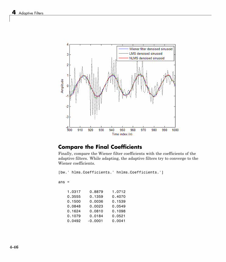
4 Adaptive Filters
Compare the Final CoefficientsFinally, compare the Wiener filter coefficients with the coefficients of theadaptive filters. While adapting, the adaptive filters try to converge to theWiener coefficients.
[bw.' hlms.Coefficients.' hnlms.Coefficients.']
ans =
1.0317 0.8879 1.07120.3555 0.1359 0.40700.1500 0.0036 0.15390.0848 0.0023 0.05490.1624 0.0810 0.10980.1079 0.0184 0.05210.0492 -0.0001 0.0041
4-46

Signal Enhancement Using LMS and Normalized LMS
Reset the Filter Before FilteringAdaptive filters have a PersistentMemory property that you can use toreproduce experiments exactly. By default, the PersistentMemory is false.The states and the coefficients of the filter are reset before filtering and thefilter does not remember the results from previous times you use the filter.
For instance, the following successive calls produce the same output whenPersistentMemory is false.
[ylms,elms] = filter(hlms,v2,x);[ylms2,elms2] = filter(hlms,v2,x);
To keep the history of the filter when filtering a new set of data, enablepersistent memory for the filter by setting the PersistentMemory propertyto true. In this configuration, the filter uses the final states and coefficientsfrom the previous run as the initial conditions for the next run and set of data.
[ylms,elms] = filter(hlms,v2,x);hlms.PersistentMemory = true;[ylms2,elms2] = filter(hlms,v2,x); % No longer the same
Setting the property value to true is useful when you are filtering largeamounts of data that you partition into smaller sets and then feed into thefilter using a for-loop construction.
Investigate Convergence Through Learning CurvesTo analyze the convergence of the adaptive filters, look at the learning curves.The toolbox provides methods to generate the learning curves, but you needmore than one iteration of the experiment to obtain significant results.
This demonstration uses 25 sample realizations of the noisy sinusoids.
n = (1:5000)';s = sin(0.075*pi*n);nr = 25;v = 0.8*randn(5000,nr);v1 = filter(1,ar,v);x = repmat(s,1,nr) + v1;v2 = filter(ma,1,v);
4-47

4 Adaptive Filters
Compute the Learning CurvesNow compute the mean-square error. To speed things up, compute the errorevery 10 samples.
First, reset the adaptive filters to avoid using the coefficients it has alreadycomputed and the states it has stored.
reset(hlms);reset(hnlms);M = 10; % Decimation factormselms = msesim(hlms,v2,x,M);msenlms = msesim(hnlms,v2,x,M);plot(1:M:n(end),[mselms,msenlms])legend('LMS learning curve','NLMS learning curve')xlabel('Time index (n)');ylabel('MSE');
In the next plot you see the calculated learning curves for the LMS andNLMS adaptive filters.
4-48

Signal Enhancement Using LMS and Normalized LMS
Compute the Theoretical Learning CurvesFor the LMS and NLMS algorithms, functions in the toolbox help you computethe theoretical learning curves, along with the minimum mean-square error(MMSE) the excess mean-square error (EMSE) and the mean value of thecoefficients.
MATLAB may take some time to calculate the curves. The figure shown afterthe code plots the predicted and actual LMS curves.
reset(hlms);[mmselms,emselms,meanwlms,pmselms] = msepred(hlms,v2,x,M);plot(1:M:n(end),[mmselms*ones(500,1),emselms*ones(500,1),...
pmselms,mselms])legend('MMSE','EMSE','predicted LMS learning curve',...
'LMS learning curve')xlabel('Time index (n)');ylabel('MSE');
4-49

4 Adaptive Filters
4-50

Adaptive Filters in Simulink®
Adaptive Filters in Simulink
In this section...
“Create an Acoustic Environment in Simulink” on page 4-51
“LMS Filter Configuration for Adaptive Noise Cancellation” on page 4-53
“Modify Adaptive Filter Parameters During Model Simulation” on page 4-59
“Adaptive Filtering Examples” on page 4-64
Create an Acoustic Environment in SimulinkAdaptive filters are filters whose coefficients or weights change over timeto adapt to the statistics of a signal. They are used in a variety of fieldsincluding communications, controls, radar, sonar, seismology, and biomedicalengineering.
In this topic, you learn how to create an acoustic environment that simulatesboth white noise and colored noise added to an input signal. You later usethis environment to build a model capable of adaptive noise cancellation usingadaptive filtering:
1 At the MATLAB command line, type dspanc.
The DSP System Toolbox Acoustic Noise Cancellation example opens.
4-51
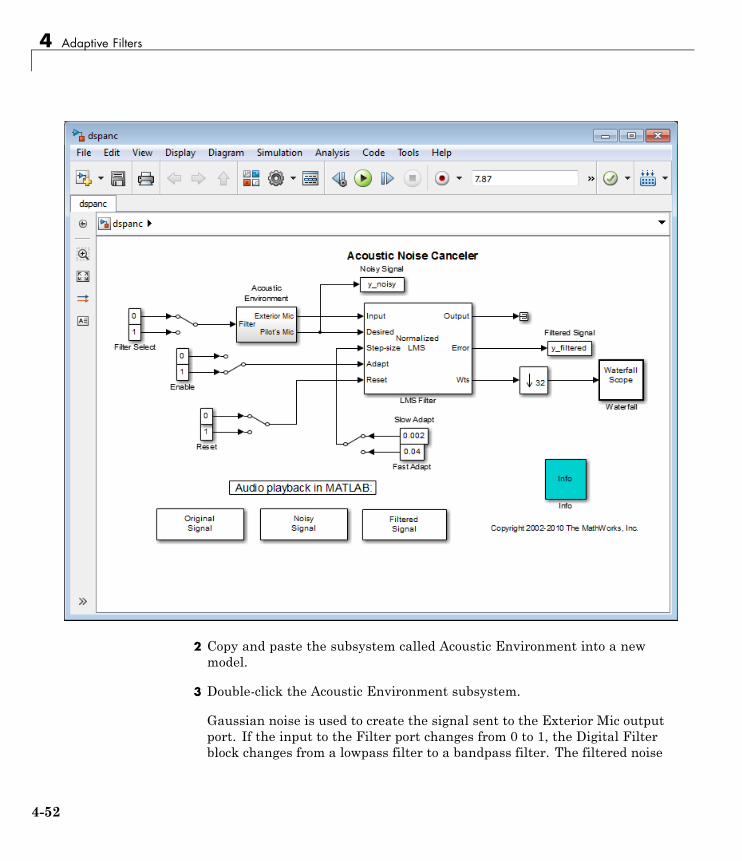
4 Adaptive Filters
2 Copy and paste the subsystem called Acoustic Environment into a newmodel.
3 Double-click the Acoustic Environment subsystem.
Gaussian noise is used to create the signal sent to the Exterior Mic outputport. If the input to the Filter port changes from 0 to 1, the Digital Filterblock changes from a lowpass filter to a bandpass filter. The filtered noise
4-52

Adaptive Filters in Simulink®
output from the Digital Filter block is added to signal coming from a .wavfile to produce the signal sent to the Pilot’s Mic output port.
You have now created an acoustic environment. In the following topics, youuse this acoustic environment to produce a model capable of adaptive noisecancellation.
LMS Filter Configuration for Adaptive NoiseCancellationIn the previous topic, “Create an Acoustic Environment in Simulink” on page4-51, you created a system that produced two output signals. The signaloutput at the Exterior Mic port is composed of white noise. The signal outputat the Pilot’s Mic port is composed of colored noise added to a signal from a.wav file. In this topic, you create an adaptive filter to remove the noise fromthe Pilot’s Mic signal. This topic assumes that you are working on a Windowsoperating system:
1 If the model you created in “Create an Acoustic Environment in Simulink”on page 4-51 is not open on your desktop, you can open an equivalentmodel by typing
ex_adapt1_audio
at the MATLAB command prompt.
2 From the DSP System Toolbox Filtering library, and then from theAdaptive Filters library, click-and-drag an LMS Filter block into the modelthat contains the Acoustic Environment subsystem.
3 Double-click the LMS Filter block. Set the block parameters as follows,and then click OK:
• Algorithm = Normalized LMS
• Filter length = 40
• Step size (mu) = 0.002
• Leakage factor (0 to 1) = 1
4-53
4 Adaptive Filters
The block uses the normalized LMS algorithm to calculate the forty filtercoefficients. Setting the Leakage factor (0 to 1) parameter to 1 meansthat the current filter coefficient values depend on the filter’s initialconditions and all of the previous input values.
4 Click-and-drag the following blocks into your model.
Block Library Quantity
Constant Simulink/Sources 2
Manual Switch Simulink/Signal Routing 1
Terminator Simulink/Sinks 1
Downsample Signal Operations 1
To Audio Device Sinks 1
Waterfall Scope Sinks 1
5 Connect the blocks so that your model resembles the following figure.
4-54

Adaptive Filters in Simulink®
6 Double-click the Constant block. Set the Constant value parameter to0 and then click OK.
7 Double-click the Downsample block. Set the Downsample factor, Kparameter to 32. Click OK.
4-55
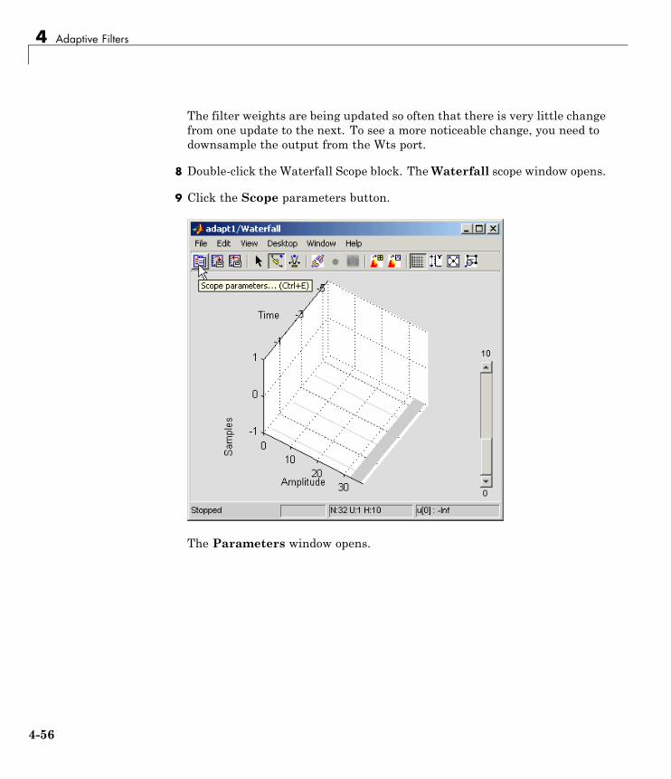
4 Adaptive Filters
The filter weights are being updated so often that there is very little changefrom one update to the next. To see a more noticeable change, you need todownsample the output from the Wts port.
8 Double-click the Waterfall Scope block. TheWaterfall scope window opens.
9 Click the Scope parameters button.
The Parameters window opens.
4-56
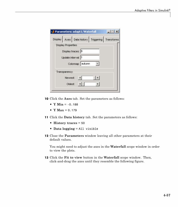
Adaptive Filters in Simulink®
10 Click the Axes tab. Set the parameters as follows:
• Y Min = -0.188
• Y Max = 0.179
11 Click the Data history tab. Set the parameters as follows:
• History traces = 50
• Data logging = All visible
12 Close the Parameters window leaving all other parameters at theirdefault values.
You might need to adjust the axes in theWaterfall scope window in orderto view the plots.
13 Click the Fit to view button in the Waterfall scope window. Then,click-and-drag the axes until they resemble the following figure.
4-57
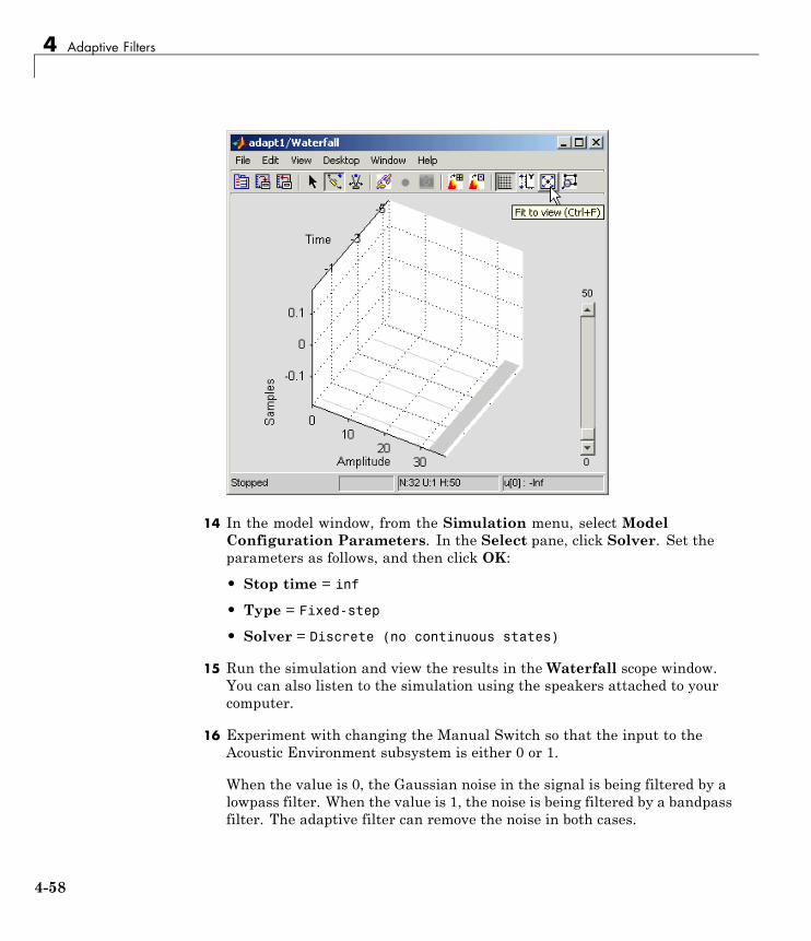
4 Adaptive Filters
14 In the model window, from the Simulation menu, select ModelConfiguration Parameters. In the Select pane, click Solver. Set theparameters as follows, and then click OK:
• Stop time = inf
• Type = Fixed-step
• Solver = Discrete (no continuous states)
15 Run the simulation and view the results in the Waterfall scope window.You can also listen to the simulation using the speakers attached to yourcomputer.
16 Experiment with changing the Manual Switch so that the input to theAcoustic Environment subsystem is either 0 or 1.
When the value is 0, the Gaussian noise in the signal is being filtered by alowpass filter. When the value is 1, the noise is being filtered by a bandpassfilter. The adaptive filter can remove the noise in both cases.
4-58

Adaptive Filters in Simulink®
You have now created a model capable of adaptive noise cancellation. Theadaptive filter in your model is able to filter out both low frequency noise andnoise within a frequency range. In the next topic, “Modify Adaptive FilterParameters During Model Simulation” on page 4-59, you modify the LMSFilter block and change its parameters during simulation.
Modify Adaptive Filter Parameters During ModelSimulationIn the previous topic, “LMS Filter Configuration for Adaptive NoiseCancellation” on page 4-53, you created an adaptive filter and used it toremove the noise generated by the Acoustic Environment subsystem. Inthis topic, you modify the adaptive filter and adjust its parameters duringsimulation. This topic assumes that you are working on a Windows operatingsystem:
1 If the model you created in “Create an Acoustic Environment in Simulink”on page 4-51 is not open on your desktop, you can open an equivalentmodel by typing
ex_adapt2_audio
at the MATLAB command prompt.
2 Double-click the LMS filter block. Set the block parameters as follows,and then click OK:
• Specify step size via = Input port
• Initial value of filter weights = 0
• Select the Adapt port check box.
• Reset port = Non-zero sample
The Block Parameters: LMS Filter dialog box should now look similarto the following figure.
4-59
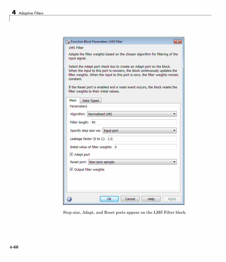
4 Adaptive Filters
Step-size, Adapt, and Reset ports appear on the LMS Filter block.
4-60
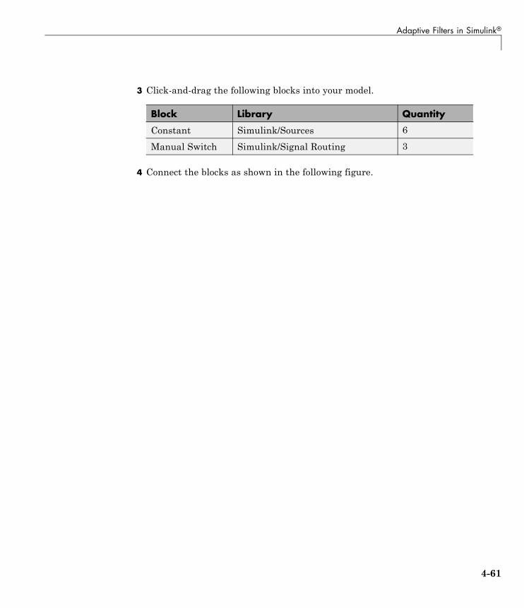
Adaptive Filters in Simulink®
3 Click-and-drag the following blocks into your model.
Block Library Quantity
Constant Simulink/Sources 6
Manual Switch Simulink/Signal Routing 3
4 Connect the blocks as shown in the following figure.
4-61

4 Adaptive Filters
4-62

Adaptive Filters in Simulink®
5 Double-click the Constant2 block. Set the block parameters as follows,and then click OK:
• Constant value = 0.002
• Select the Interpret vector parameters as 1-D check box.
• Sample time (-1 for inherited) = inf
• Output data type mode = Inherit via back propagation
6 Double-click the Constant3 block. Set the block parameters as follows,and then click OK:
• Constant value = 0.04
• Select the Interpret vector parameters as 1-D check box.
• Sample time (-1 for inherited) = inf
• Output data type mode = Inherit via back propagation
7 Double-click the Constant4 block. Set the Constant value parameter to0 and then click OK.
8 Double-click the Constant6 block. Set the Constant value parameter to0 and then click OK.
9 In the model window, from the Display menu, point to Signals & Ports,and select Wide Nonscalar Lines and Signal Dimensions.
10 Double-click Manual Switch2 so that the input to the Adapt port is 1.
11 Run the simulation and view the results in the Waterfall scope window.You can also listen to the simulation using the speakers attached to yourcomputer.
12 Double-click the Manual Switch block so that the input to the AcousticEnvironment subsystem is 1. Then, double-click Manual Switch2 so thatthe input to the Adapt port to 0.
The filter weights displayed in the Waterfall scope window remainconstant. When the input to the Adapt port is 0, the filter weights arenot updated.
4-63

4 Adaptive Filters
13 Double-click Manual Switch2 so that the input to the Adapt port is 1.
The LMS Filter block updates the coefficients.
14 Connect the Manual Switch1 block to the Constant block that represents0.002. Then, change the input to the Acoustic Environment subsystem.Repeat this procedure with the Constant block that represents 0.04.
You can see that the system reaches steady state faster when the stepsize is larger.
15 Double-click the Manual Switch3 block so that the input to the Reset portis 1.
The block resets the filter weights to their initial values. In the BlockParameters: LMS Filter dialog box, from the Reset port list, you choseNon-zero sample. This means that any nonzero input to the Reset porttriggers a reset operation.
You have now experimented with adaptive noise cancellation using the LMSFilter block. You adjusted the parameters of your adaptive filter and viewedthe effects of your changes while the model was running.
For more information about adaptive filters, see the following block referencepages:
• LMS Filter
• RLS Filter
• Block LMS Filter
• Fast Block LMS Filter
Adaptive Filtering ExamplesDSP System Toolbox software provides a collection of adaptive filteringexamples that illustrate typical applications of the adaptive filtering blocks,listed in the following table.
4-64
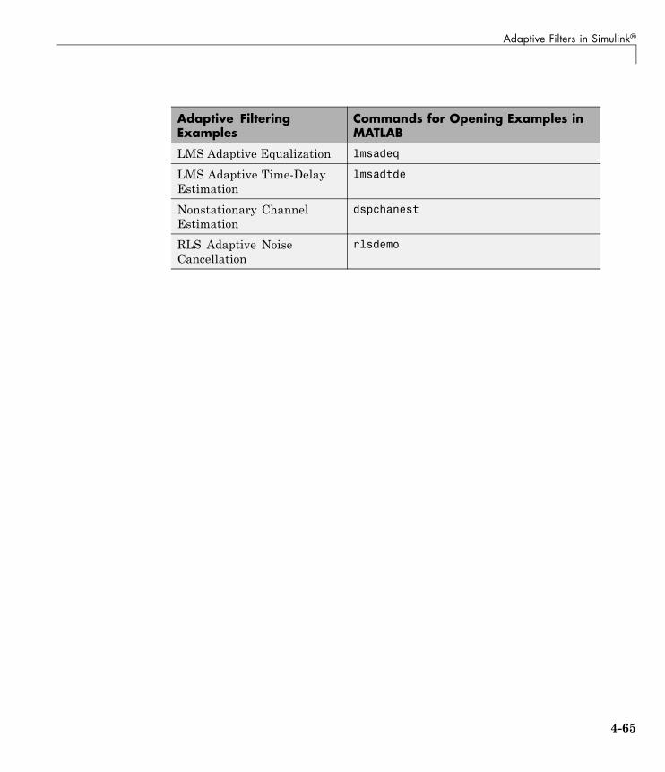
Adaptive Filters in Simulink®
Adaptive FilteringExamples
Commands for Opening Examples inMATLAB
LMS Adaptive Equalization lmsadeq
LMS Adaptive Time-DelayEstimation
lmsadtde
Nonstationary ChannelEstimation
dspchanest
RLS Adaptive NoiseCancellation
rlsdemo
4-65
4 Adaptive Filters
Selected Bibliography[1] Hayes, Monson H., Statistical Digital Signal Processing and Modeling,John Wiley & Sons, 1996, 493–552.
[2] Haykin, Simon, Adaptive Filter Theory, Prentice-Hall, Inc., 1996
4-66

5
Multirate and MultistageFilters
Learn how to analyze, design, and implement multirate and multistage filtersin MATLAB and Simulink.
• “Multirate Filters” on page 5-2
• “Multistage Filters” on page 5-6
• “Example Case for Multirate/Multistage Filters” on page 5-8
• “Filter Banks” on page 5-12
• “Multirate Filtering in Simulink” on page 5-21

5 Multirate and Multistage Filters
Multirate Filters
In this section...
“Why Are Multirate Filters Needed?” on page 5-2
“Overview of Multirate Filters” on page 5-2
Why Are Multirate Filters Needed?Multirate filters can bring efficiency to a particular filter implementation.In general, multirate filters are filters in which different parts of the filteroperate at different rates. The most obvious application of such a filter iswhen the input sample rate and output sample rate need to differ (decimationor interpolation) — however, multirate filters are also often used in designswhere this is not the case. For example you may have a system where theinput sample rate and output sample rate are the same, but internally thereis decimation and interpolation occurring in a series of filters, such that thefinal output of the system has the same sample rate as the input. Such adesign may exhibit lower cost than could be achieved with a single-rate filterfor various reasons. For more information about the relative cost benefitof using multirate filters, refer to [2] Harris, Fredric J., Multirate SignalProcessing for Communication Systems, Prentice Hall PTR, 2004.
Overview of Multirate FiltersA filter that reduces the input rate is called a decimator. A filter thatincreases the input rate is called an interpolator. To visualize this process,examine the following figure, which illustrates the processes of interpolationand decimation in the time domain.
5-2
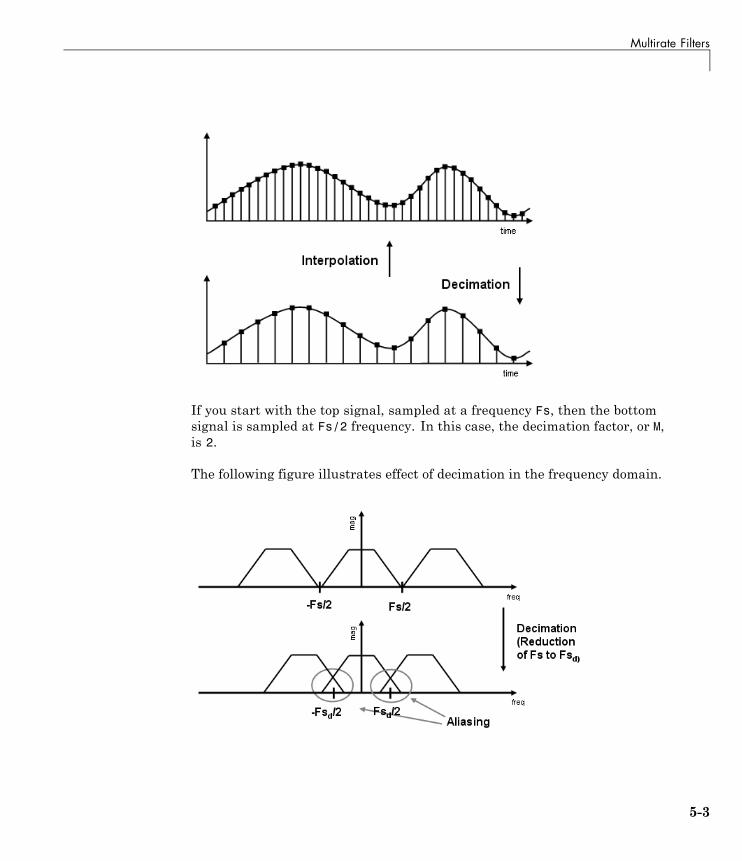
Multirate Filters
If you start with the top signal, sampled at a frequency Fs, then the bottomsignal is sampled at Fs/2 frequency. In this case, the decimation factor, or M,is 2.
The following figure illustrates effect of decimation in the frequency domain.
5-3
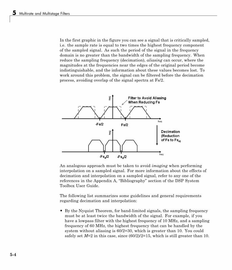
5 Multirate and Multistage Filters
In the first graphic in the figure you can see a signal that is critically sampled,i.e. the sample rate is equal to two times the highest frequency componentof the sampled signal. As such the period of the signal in the frequencydomain is no greater than the bandwidth of the sampling frequency. Whenreduce the sampling frequency (decimation), aliasing can occur, where themagnitudes at the frequencies near the edges of the original period becomeindistinguishable, and the information about these values becomes lost. Towork around this problem, the signal can be filtered before the decimationprocess, avoiding overlap of the signal spectra at Fs/2.
An analogous approach must be taken to avoid imaging when performinginterpolation on a sampled signal. For more information about the effects ofdecimation and interpolation on a sampled signal, refer to any one of thereferences in the Appendix A, “Bibliography” section of the DSP SystemToolbox User Guide.
The following list summarizes some guidelines and general requirementsregarding decimation and interpolation:
• By the Nyquist Theorem, for band-limited signals, the sampling frequencymust be at least twice the bandwidth of the signal. For example, if youhave a lowpass filter with the highest frequency of 10 MHz, and a samplingfrequency of 60 MHz, the highest frequency that can be handled by thesystem without aliasing is 60/2=30, which is greater than 10. You couldsafely set M=2 in this case, since (60/2)/2=15, which is still greater than 10.
5-4
Multirate Filters
• If you wish to decimate a signal which does not meet the frequency criteria,you can either:
- Interpolate first, and then decimate
- When decimating, you should apply the filter first, then perform thedecimation. When interpolating a signal, you should interpolate first,then filter the signal.
• Typically in decimation of a signal a filter is applied first, thereby allowingdecimation without aliasing, as shown in the following figure:
• Conversely, a filter is typically applied after interpolation to avoid imaging:
• M must be an integer. Although, if you wish to obtain an M of 4/5, youcould interpolate by 4, and then decimate by 5, provided that frequencyrestrictions are met. This type of multirate filter will be referred to as asample rate converter in the documentation that follows.
Multirate filters are most often used in stages. This technique is introducedin the following section.
5-5

5 Multirate and Multistage Filters
Multistage Filters
In this section...
“Why Are Multistage Filters Needed?” on page 5-6
“Optimal Multistage Filters in DSP System Toolbox” on page 5-6
Why Are Multistage Filters Needed?Typically used with multirate filters, multistage filters can bring efficiencyto a particular filter implementation. Multistage filters are composed ofseveral filters. These different parts of the mulitstage filter, called stages, areconnected in a cascade or in parallel. However such a design can conserveresources in many cases. There are many different uses for a multistage filter.One of these is a filter requirement that includes a very narrow transitionwidth. For example, you need to design a lowpass filter where the differencebetween the pass frequency and the stop frequency is .01 (normalized).For such a requirement it is possible to design a single filter, but it willbe very long (containing many coefficients) and very costly (having manymultiplications and additions per input sample). Thus, this single filtermay be so costly and require so much memory, that it may be impracticalto implement in certain applications where there are strict hardwarerequirements. In such cases, a multistage filter is a great solution. Anotherapplication of a multistage filter is for a mulitrate system, where there is adecimator or an interpolator with a large factor. In these cases, it is usuallywise to break up the filter into several multirate stages, each comprising amultiple of the total decimation/interpolation factor.
Optimal Multistage Filters in DSP System ToolboxAs described in the previous section, within a multirate filter eachinterconnected filter is called a stage. While it is possible to designa multistage filter manually, it is also possible to perform automaticoptimization of a multistage filter automatically. When designing a filtermanually it can be difficult to guess how many stages would provide anoptimal design, optimize each stage, and then optimize all the stages together.DSP System Toolbox software enables you to create a Specifications Object,and then design a filter using multistage as an option. The rest of the work is
5-6

Multistage Filters
done automatically. Not only does DSP System Toolbox software determinethe optimal number of stages, but it also optimizes the total filter solution.
5-7

5 Multirate and Multistage Filters
Example Case for Multirate/Multistage Filters
In this section...
“Example Overview” on page 5-8
“Single-Rate/Single-Stage Equiripple Design” on page 5-8
“Reduce Computational Cost Using Mulitrate/Multistage Design” on page5-9
“Compare the Responses” on page 5-9
“Further Performance Comparison” on page 5-10
Example OverviewThis example shows the efficiency gains that are possible when usingmultirate and multistage filters for certain applications. In this case a distinctadvantage is achieved over regular linear-phase equiripple design when anarrow transition-band width is required. A more detailed treatment of thekey points made here can be found in the example entitled Efficient NarrowTransition-Band FIR Filter Design.
Single-Rate/Single-Stage Equiripple DesignConsider the following design specifications for a lowpass filter (where theripples are given in linear units):
Fpass = 0.13; % Passband edge
Fstop = 0.14; % Stopband edge
Rpass = 0.001; % Passband ripple, 0.0174 dB peak to peak
Rstop = 0.0005; % Stopband ripple, 66.0206 dB minimum attenuation
Hf = fdesign.lowpass(Fpass,Fstop,Rpass,Rstop,'linear');
A regular linear-phase equiripple design using these specifications can bedesigned by evaluating the following:
Hd = design(Hf,'equiripple');
5-8

Example Case for Multirate/Multistage Filters
When you determine the cost of this design, you can see that 695 multipliersare required.
cost(Hd)
Reduce Computational Cost UsingMulitrate/Multistage DesignThe number of multipliers required by a filter using a single state,single rate equiripple design is 694. This number can be reduced usingmultirate/multistage techniques. In any single-rate design, the numberof multiplications required by each input sample is equal to the numberof non-zero multipliers in the implementation. However, by using amultirate/multistage design, decimation and interpolation can be combinedto lessen the computation required. For decimators, the average numberof multiplications required per input sample is given by the number ofmultipliers divided by the decimation factor.
Hd_multi = design(Hf,'multistage');
You can then view the cost of the filter created using this design step, and youcan see that a significant cost advantage has been achieved.
cost(Hd_multi)
Compare the ResponsesYou can compare the responses of the equiripple design and thismultirate/multistage design using fvtool:
hfvt = fvtool(Hd,Hd_multi);legend(hfvt,'Equiripple design', 'Multirate/multistage design')
5-9

5 Multirate and Multistage Filters
Notice that the stopband attenuation for the multistage design is about twicethat of the other designs. This is because the decimators must attenuateout-of-band components by 66 dB in order to avoid aliasing that would violatethe specifications. Similarly, the interpolators must attenuate images by66 dB. You can also see that the passband gain for this design is no longer0 dB, because each interpolator has a nominal gain (in linear units) equalto its interpolation factor, and the total interpolation factor for the threeinterpolators is 6.
Further Performance ComparisonYou can check the performance of the multirate/multistage design by plottingthe power spectral densities of the input and the various outputs, and you can
see that the sinusoid at 0 4. π is attenuated comparably by both the equirippledesign and the multirate/multistage design.
n = 0:1799;x = sin(0.1*pi*n') + 2*sin(0.15*pi*n');y = filter(Hd,x);
5-10
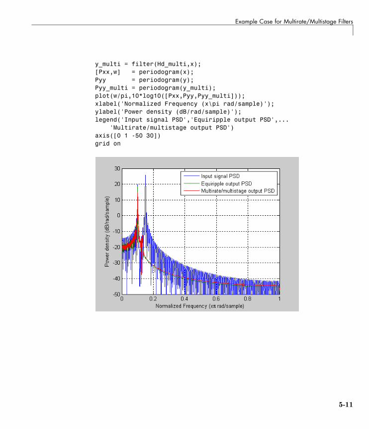
Example Case for Multirate/Multistage Filters
y_multi = filter(Hd_multi,x);[Pxx,w] = periodogram(x);Pyy = periodogram(y);Pyy_multi = periodogram(y_multi);plot(w/pi,10*log10([Pxx,Pyy,Pyy_multi]));xlabel('Normalized Frequency (x\pi rad/sample)');ylabel('Power density (dB/rad/sample)');legend('Input signal PSD','Equiripple output PSD',...
'Multirate/multistage output PSD')axis([0 1 -50 30])grid on
5-11

5 Multirate and Multistage Filters
Filter BanksMultirate filters alter the sample rate of the input signal during the filteringprocess. Such filters are useful in both rate conversion and filter bankapplications.
The Dyadic Analysis Filter Bank block decomposes a broadband signal into acollection of subbands with smaller bandwidths and slower sample rates. TheDyadic Synthesis Filter Bank block reconstructs a signal decomposed by theDyadic Analysis Filter Bank block.
To use a dyadic synthesis filter bank to perfectly reconstruct the output of adyadic analysis filter bank, the number of levels and tree structures of bothfilter banks must be the same. In addition, the filters in the synthesis filterbank must be designed to perfectly reconstruct the outputs of the analysisfilter bank. Otherwise, the reconstruction will not be perfect.
Dyadic Analysis Filter BanksDyadic analysis filter banks are constructed from the following basic unit.The unit can be cascaded to construct dyadic analysis filter banks with eithera symmetric or asymmetric tree structure.
Each unit consists of a lowpass (LP) and highpass (HP) FIR filter pair,followed by a decimation by a factor of 2. The filters are halfband filters witha cutoff frequency of Fs / 4, a quarter of the input sampling frequency. Eachfilter passes the frequency band that the other filter stops.
The unit decomposes its input into adjacent high-frequency and low-frequencysubbands. Compared to the input, each subband has half the bandwidth (dueto the half-band filters) and half the sample rate (due to the decimation by 2).
5-12
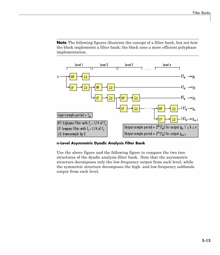
Filter Banks
Note The following figures illustrate the concept of a filter bank, but not howthe block implements a filter bank; the block uses a more efficient polyphaseimplementation.
n-Level Asymmetric Dyadic Analysis Filter Bank
Use the above figure and the following figure to compare the two treestructures of the dyadic analysis filter bank. Note that the asymmetricstructure decomposes only the low-frequency output from each level, whilethe symmetric structure decomposes the high- and low-frequency subbandsoutput from each level.
5-13
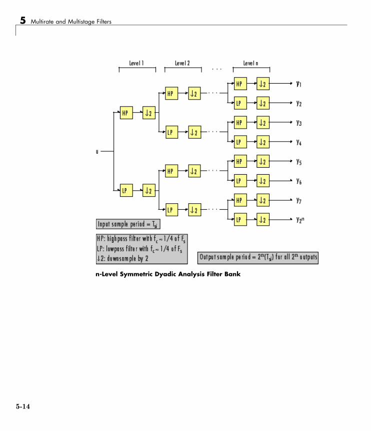
5 Multirate and Multistage Filters
n-Level Symmetric Dyadic Analysis Filter Bank
5-14
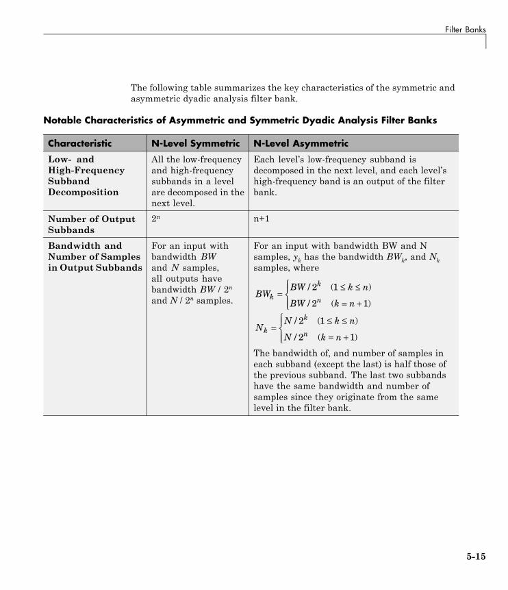
Filter Banks
The following table summarizes the key characteristics of the symmetric andasymmetric dyadic analysis filter bank.
Notable Characteristics of Asymmetric and Symmetric Dyadic Analysis Filter Banks
Characteristic N-Level Symmetric N-Level Asymmetric
Low- andHigh-FrequencySubbandDecomposition
All the low-frequencyand high-frequencysubbands in a levelare decomposed in thenext level.
Each level’s low-frequency subband isdecomposed in the next level, and each level’shigh-frequency band is an output of the filterbank.
Number of OutputSubbands
2n n+1
Bandwidth andNumber of Samplesin Output Subbands
For an input withbandwidth BWand N samples,all outputs havebandwidth BW / 2n
and N / 2n samples.
For an input with bandwidth BW and Nsamples, yk has the bandwidth BWk, and Nksamples, where
BWBW k n
BW k nk
k
n=
≤ ≤
= +
⎧⎨⎪
⎩⎪
/ ( )
/ ( )
2 1
2 1
NN k n
N k nk
k
n=
≤ ≤
= +
⎧⎨⎪
⎩⎪
/ ( )
/ ( )
2 1
2 1
The bandwidth of, and number of samples ineach subband (except the last) is half those ofthe previous subband. The last two subbandshave the same bandwidth and number ofsamples since they originate from the samelevel in the filter bank.
5-15

5 Multirate and Multistage Filters
Notable Characteristics of Asymmetric and Symmetric Dyadic Analysis Filter Banks(Continued)
Characteristic N-Level Symmetric N-Level Asymmetric
Output SamplePeriod
All output subbandshave a sample periodof 2n(Tsi)
Sample period of kth output
=≤ ≤
= +
⎧⎨⎪
⎩⎪
2 1
2 1
ksi
nsi
T k n
T k n
( ) ( )
( ) ( )
Due to the decimations by 2, the sample periodof each subband (except the last) is twice thatof the previous subband. The last two subbandshave the same sample period since theyoriginate from the same level in the filter bank.
Total Number ofOutput Samples
The total number of samples in all of the output subbands is equal tothe number of samples in the input (due to the of decimations by 2 ateach level).
WaveletApplications
In wavelet applications, the highpass and lowpass wavelet-based filtersare designed so that the aliasing introduced by the decimations areexactly canceled in reconstruction.
Dyadic Synthesis Filter BanksDyadic synthesis filter banks are constructed from the following basic unit.The unit can be cascaded to construct dyadic synthesis filter banks with eithera asymmetric or symmetric tree structure as illustrated in the figures entitledn-Level Asymmetric Dyadic Synthesis Filter Bank and n-Level SymmetricDyadic Synthesis Filter Bank.
Each unit consists of a lowpass (LP) and highpass (HP) FIR filter pair,preceded by an interpolation by a factor of 2. The filters are halfband filterswith a cutoff frequency of Fs / 4, a quarter of the input sampling frequency.Each filter passes the frequency band that the other filter stops.
5-16
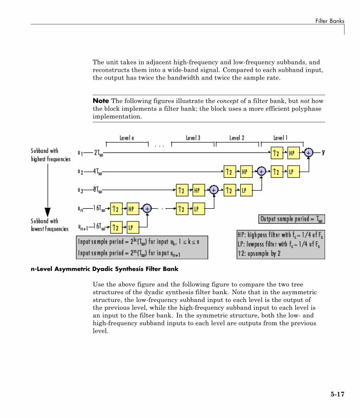
Filter Banks
The unit takes in adjacent high-frequency and low-frequency subbands, andreconstructs them into a wide-band signal. Compared to each subband input,the output has twice the bandwidth and twice the sample rate.
Note The following figures illustrate the concept of a filter bank, but not howthe block implements a filter bank; the block uses a more efficient polyphaseimplementation.
n-Level Asymmetric Dyadic Synthesis Filter Bank
Use the above figure and the following figure to compare the two treestructures of the dyadic synthesis filter bank. Note that in the asymmetricstructure, the low-frequency subband input to each level is the output ofthe previous level, while the high-frequency subband input to each level isan input to the filter bank. In the symmetric structure, both the low- andhigh-frequency subband inputs to each level are outputs from the previouslevel.
5-17
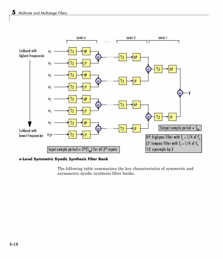
5 Multirate and Multistage Filters
n-Level Symmetric Dyadic Synthesis Filter Bank
The following table summarizes the key characteristics of symmetric andasymmetric dyadic synthesis filter banks.
5-18
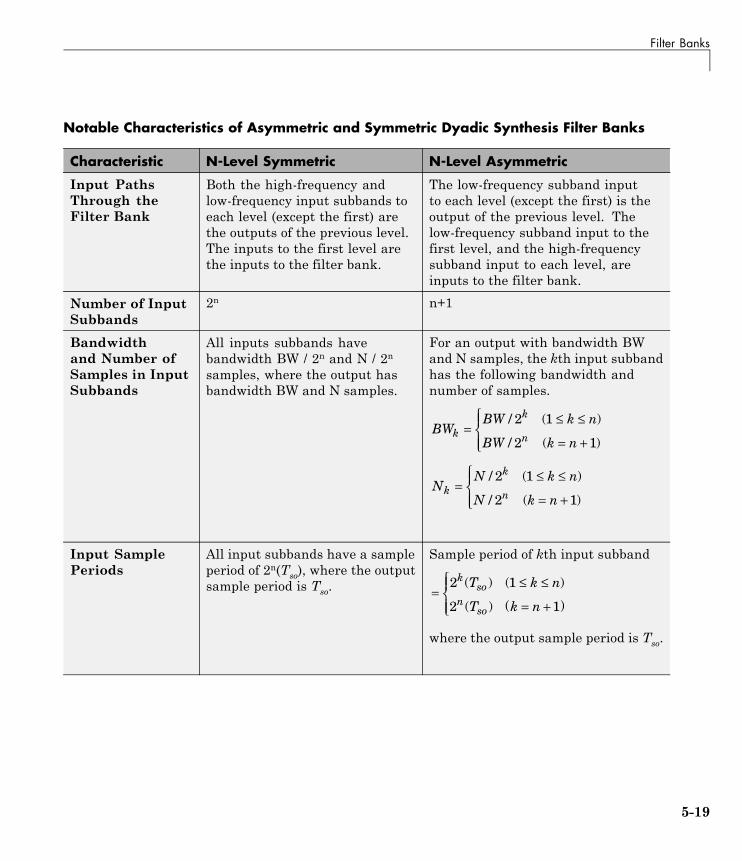
Filter Banks
Notable Characteristics of Asymmetric and Symmetric Dyadic Synthesis Filter Banks
Characteristic N-Level Symmetric N-Level Asymmetric
Input PathsThrough theFilter Bank
Both the high-frequency andlow-frequency input subbands toeach level (except the first) arethe outputs of the previous level.The inputs to the first level arethe inputs to the filter bank.
The low-frequency subband inputto each level (except the first) is theoutput of the previous level. Thelow-frequency subband input to thefirst level, and the high-frequencysubband input to each level, areinputs to the filter bank.
Number of InputSubbands
2n n+1
Bandwidthand Number ofSamples in InputSubbands
All inputs subbands havebandwidth BW / 2n and N / 2n
samples, where the output hasbandwidth BW and N samples.
For an output with bandwidth BWand N samples, the kth input subbandhas the following bandwidth andnumber of samples.
BWBW k n
BW k nk
k
n=
≤ ≤
= +
⎧⎨⎪
⎩⎪
/ ( )
/ ( )
2 1
2 1
NN k n
N k nk
k
n=
≤ ≤
= +
⎧⎨⎪
⎩⎪
/ ( )
/ ( )
2 1
2 1
Input SamplePeriods
All input subbands have a sampleperiod of 2n(Tso), where the outputsample period is Tso.
Sample period of kth input subband
=≤ ≤
= +( )
⎧⎨⎪
⎩⎪
2 1
2 1
kso
nso
T k n
T k n
( ) ( )
( )
where the output sample period is Tso.
5-19
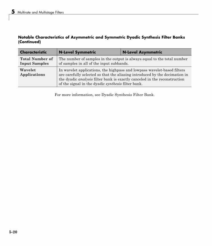
5 Multirate and Multistage Filters
Notable Characteristics of Asymmetric and Symmetric Dyadic Synthesis Filter Banks(Continued)
Characteristic N-Level Symmetric N-Level Asymmetric
Total Number ofInput Samples
The number of samples in the output is always equal to the total numberof samples in all of the input subbands.
WaveletApplications
In wavelet applications, the highpass and lowpass wavelet-based filtersare carefully selected so that the aliasing introduced by the decimation inthe dyadic analysis filter bank is exactly canceled in the reconstructionof the signal in the dyadic synthesis filter bank.
For more information, see Dyadic Synthesis Filter Bank.
5-20
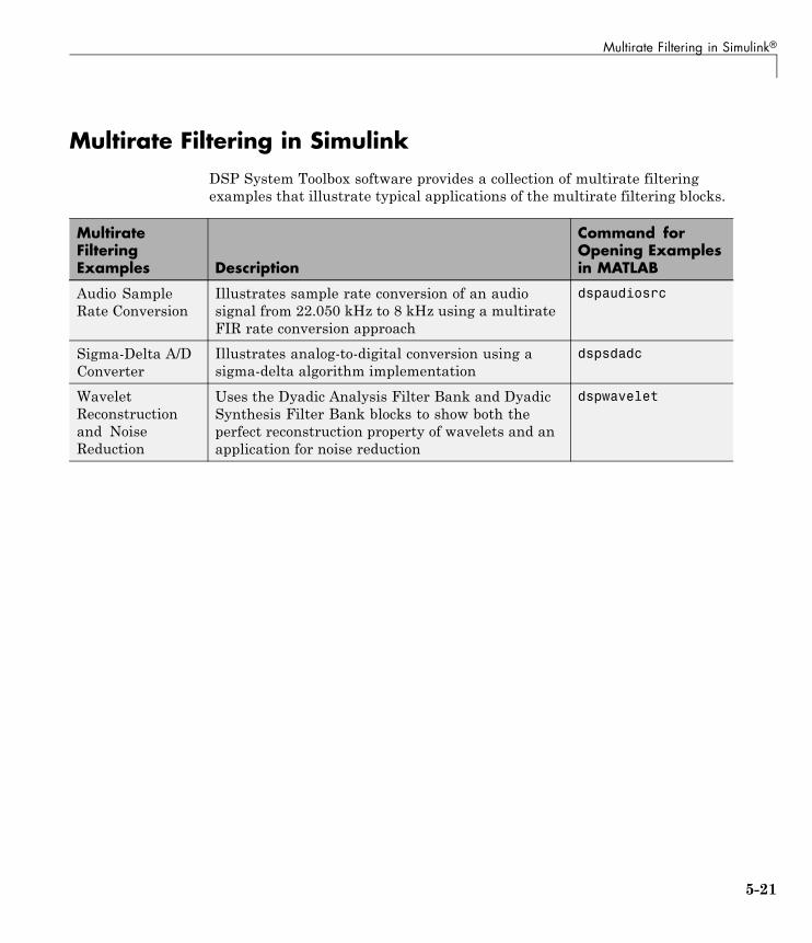
Multirate Filtering in Simulink®
Multirate Filtering in SimulinkDSP System Toolbox software provides a collection of multirate filteringexamples that illustrate typical applications of the multirate filtering blocks.
MultirateFilteringExamples Description
Command forOpening Examplesin MATLAB
Audio SampleRate Conversion
Illustrates sample rate conversion of an audiosignal from 22.050 kHz to 8 kHz using a multirateFIR rate conversion approach
dspaudiosrc
Sigma-Delta A/DConverter
Illustrates analog-to-digital conversion using asigma-delta algorithm implementation
dspsdadc
WaveletReconstructionand NoiseReduction
Uses the Dyadic Analysis Filter Bank and DyadicSynthesis Filter Bank blocks to show both theperfect reconstruction property of wavelets and anapplication for noise reduction
dspwavelet
5-21

5 Multirate and Multistage Filters
5-22

6
Transforms, Estimation,and Spectral Analysis
Learn about transforms, estimation and spectral analysis.
• “Transform Time-Domain Data into Frequency Domain” on page 6-2
• “Transform Frequency-Domain Data into Time Domain” on page 6-7
• “Linear and Bit-Reversed Output Order” on page 6-13
• “Calculate Channel Latencies Required for Wavelet Reconstruction” onpage 6-15
• “Spectral Analysis” on page 6-24
• “Power Spectrum Estimates” on page 6-25
• “Spectrograms” on page 6-36

6 Transforms, Estimation, and Spectral Analysis
Transform Time-Domain Data into Frequency DomainWhen you want to transform time-domain data into the frequency domain,use the FFT block.
In this example, you use the Sine Wave block to generate two sinusoids, oneat 15 Hz and the other at 40 Hz. You sum the sinusoids point-by-point togenerate the compound sinusoid
u t t= ( ) + ( )sin sin30 80
Then, you transform this sinusoid into the frequency domain using an FFTblock:
1 At the MATLAB command prompt, type ex_fft_tut.
The FFT Example opens.
6-2
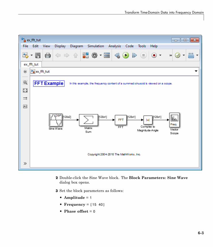
Transform Time-Domain Data into Frequency Domain
2 Double-click the Sine Wave block. The Block Parameters: Sine Wavedialog box opens.
3 Set the block parameters as follows:
• Amplitude = 1
• Frequency = [15 40]
• Phase offset = 0
6-3

6 Transforms, Estimation, and Spectral Analysis
• Sample time = 0.001
• Samples per frame = 128
Based on these parameters, the Sine Wave block outputs two sinusoidalsignals with identical amplitudes, phases, and sample times. One sinusoidoscillates at 15 Hz and the other at 40 Hz.
4 Save these parameters and close the dialog box by clicking OK.
5 Double-click the Matrix Sum block. The Block Parameters: Matrix Sumdialog box opens.
6 Set the Sum over parameter to Specified dimension and theDimensionparameter to 2. Click OK to save your changes.
Because each column represents a different signal, you need to sum alongthe individual rows in order to add the values of the sinusoids at eachtime step.
7 Double-click the Complex to Magnitude-Angle block. The BlockParameters: Complex to Magnitude-Angle dialog box opens.
8 Set the Output parameter to Magnitude, and then click OK.
This block takes the complex output of the FFT block and converts thisoutput to magnitude.
9 Double-click the Vector Scope block.
10 Set the block parameters as follows, and then click OK:
• Click the Scope Properties tab.
• Input domain = Frequency
• Click the Axis Properties tab.
• Frequency units = Hertz (This corresponds to the units of the inputsignals.)
• Frequency range = [0...Fs/2]
• Select the Inherit sample time from input check box.
• Amplitude scaling = Magnitude
6-4
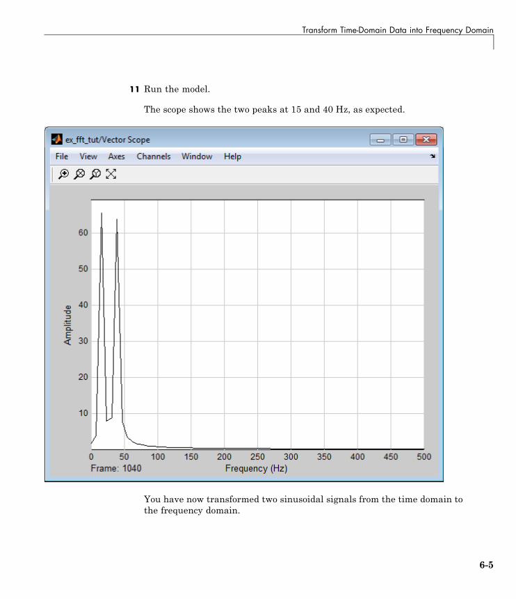
Transform Time-Domain Data into Frequency Domain
11 Run the model.
The scope shows the two peaks at 15 and 40 Hz, as expected.
You have now transformed two sinusoidal signals from the time domain tothe frequency domain.
6-5

6 Transforms, Estimation, and Spectral Analysis
Note that the sequence of FFT, Complex to Magnitude-Angle, and VectorScope blocks could be replaced by a single Spectrum Analyzer block, whichcomputes the magnitude FFT internally. Other blocks that compute the FFTinternally are the blocks in the Power Spectrum Estimation library. See“Spectral Analysis” on page 6-24 for more information about these blocks.
6-6

Transform Frequency-Domain Data into Time Domain
Transform Frequency-Domain Data into Time DomainWhen you want to transform frequency-domain data into the time domain,use the IFFT block.
In this example, you use the Sine Wave block to generate two sinusoids, oneat 15 Hz and the other at 40 Hz. You sum the sinusoids point-by-point to
generate the compound sinusoid, u t t= ( ) +sin sin( )30 80 . You transformthis sinusoid into the frequency domain using an FFT block, and thenimmediately transform the frequency-domain signal back to the time domainusing the IFFT block. Lastly, you plot the difference between the originaltime-domain signal and transformed time-domain signal using a scope:
1 At the MATLAB command prompt, type ex_ifft_tut.
The IFFT Example opens.
6-7
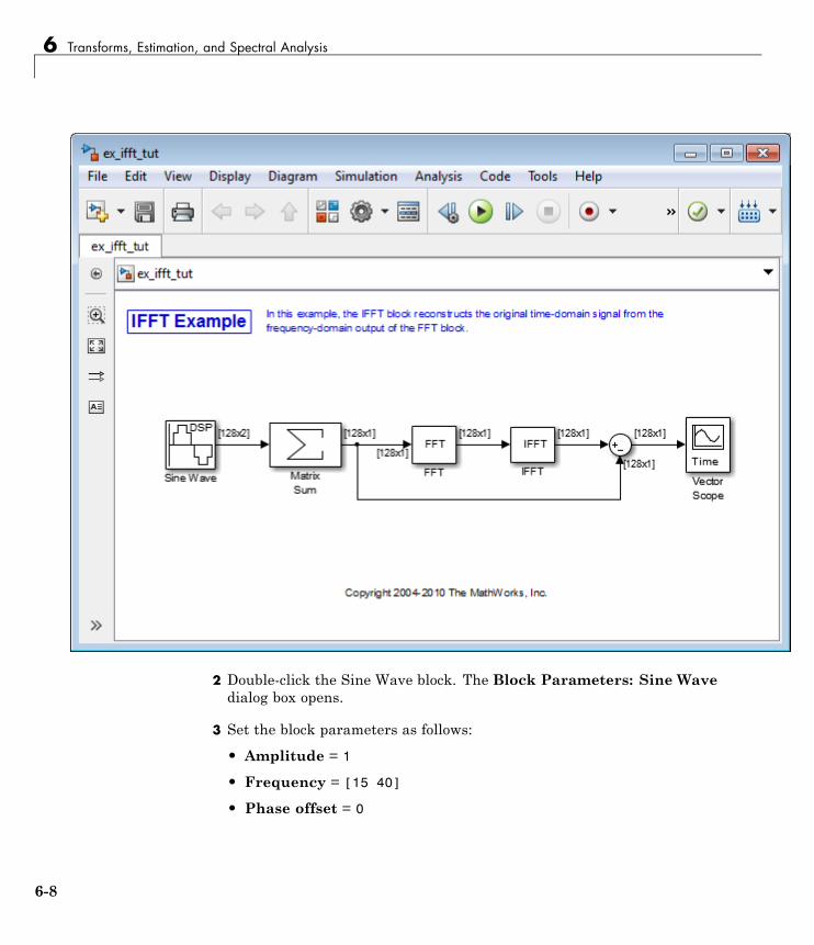
6 Transforms, Estimation, and Spectral Analysis
2 Double-click the Sine Wave block. The Block Parameters: Sine Wavedialog box opens.
3 Set the block parameters as follows:
• Amplitude = 1
• Frequency = [15 40]
• Phase offset = 0
6-8
Transform Frequency-Domain Data into Time Domain
• Sample time = 0.001
• Samples per frame = 128
Based on these parameters, the Sine Wave block outputs two sinusoidalsignals with identical amplitudes, phases, and sample times. One sinusoidoscillates at 15 Hz and the other at 40 Hz.
4 Save these parameters and close the dialog box by clicking OK.
5 Double-click the Matrix Sum block. The Block Parameters: Matrix Sumdialog box opens.
6 Set the Sum over parameter to Specified dimension and theDimensionparameter to 2. Click OK to save your changes.
Because each column represents a different signal, you need to sum alongthe individual rows in order to add the values of the sinusoids at eachtime step.
7 Double-click the FFT block. The Block Parameters: FFT dialog boxopens.
8 Select the Output in bit-reversed order check box., and then click OK.
9 Double-click the IFFT block. The Block Parameters: IFFT dialog boxopens.
10 Set the block parameters as follows, and then click OK:
• Select the Input is in bit-reversed order check box.
• Select the Input is conjugate symmetric check box.
Because the original sinusoidal signal is real valued, the output of the FFTblock is conjugate symmetric. By conveying this information to the IFFTblock, you optimize its operation.
Note that the Sum block subtracts the original signal from the output ofthe IFFT block, which is the estimation of the original signal.
11 Double-click the Vector Scope block.
12 Set the block parameters as follows, and then click OK:
6-9

6 Transforms, Estimation, and Spectral Analysis
• Click the Scope Properties tab.
• Input domain = Time
13 Run the model.
The flat line on the scope suggests that there is no difference between theoriginal signal and the estimate of the original signal. Therefore, the IFFT
6-10

Transform Frequency-Domain Data into Time Domain
block has accurately reconstructed the original time-domain signal fromthe frequency-domain input.
6-11

6 Transforms, Estimation, and Spectral Analysis
14 Right-click in the Vector Scope window, and select Autoscale.
In actuality, the two signals are identical to within round-off error. Theprevious figure shows the enlarged trace. The differences between thetwo signals is on the order of 10-15.
6-12

Linear and Bit-Reversed Output Order
Linear and Bit-Reversed Output Order
In this section...
“FFT and IFFT Blocks Data Order” on page 6-13
“Find the Bit-Reversed Order of Your Frequency Indices” on page 6-13
FFT and IFFT Blocks Data OrderThe FFT block enables you to output the frequency indices in linear orbit-reversed order. Because linear ordering of the frequency indices requires abit-reversal operation, the FFT block may run more quickly when the outputfrequencies are in bit-reversed order.
The input to the IFFT block can be in linear or bit-reversed order. Therefore,you do not have to alter the ordering of your data before transforming it backinto the time domain. However, the IFFT block may run more quickly whenthe input is provided in bit-reversed order.
Find the Bit-Reversed Order of Your FrequencyIndicesTwo numbers are bit-reversed values of each other when the binaryrepresentation of one is the mirror image of the binary representation ofthe other. For example, in a three-bit system, one and four are bit-reversedvalues of each other, since the three-bit binary representation of one, 001, isthe mirror image of the three-bit binary representation of four, 100. In thediagram below, the frequency indices are in linear order. To put them inbit-reversed order
1 Translate the indices into their binary representation with the minimumnumber of bits. In this example, the minimum number of bits is threebecause the binary representation of 7 is 111.
2 Find the mirror image of each binary entry, and write it beside the originalbinary representation.
3 Translate the indices back to their decimal representation.
6-13

6 Transforms, Estimation, and Spectral Analysis
The frequency indices are now in bit-reversed order.
The next diagram illustrates the linear and bit-reversed outputs of the FFTblock. The output values are the same, but they appear in different order.
6-14
Calculate Channel Latencies Required for Wavelet Reconstruction
Calculate Channel Latencies Required for WaveletReconstruction
In this section...
“Analyze Your Model” on page 6-15
“Calculate the Group Delay of Your Filters” on page 6-17
“Reconstruct the Filter Bank System” on page 6-19
“Equalize the Delay on Each Filter Path” on page 6-20
“Update and Run the Model” on page 6-22
“References” on page 6-23
Analyze Your ModelThe following sections guide you through the process of calculating thechannel latencies required for perfect wavelet reconstruction. This exampleuses the ex_wavelets model, but you can apply the process to perform perfectwavelet reconstruction in any model. To open the example model, typeex_wavelets at the MATLAB command line.
Note You must have a Wavelet Toolbox™ product license to run theex_wavelets model.
6-15

6 Transforms, Estimation, and Spectral Analysis
Before you can begin calculating the latencies required for perfect waveletreconstruction, you must know the types of filters being used in your model.
The Dyadic Analysis Filter Bank and the Dyadic Synthesis Filter Bank blocksin the ex_wavelets model have the following settings:
• Filter = Biorthogonal
• Filter order [synthesis/analysis] = [3/5]
• Number of levels = 3
• Tree structure = Asymmetric
• Input = Multiple ports
6-16
Calculate Channel Latencies Required for Wavelet Reconstruction
Based on these settings, the Dyadic Analysis Filter Bank and the DyadicSynthesis Filter Bank blocks construct biorthogonal filters using the WaveletToolbox wfilters function.
Calculate the Group Delay of Your FiltersOnce you know the types of filters being used by the Dyadic Analysis andDyadic Synthesis Filter Bank blocks, you need to calculate the group delay ofthose filters. To do so, you can use the Signal Processing Toolbox fvtool.
Before you can use fvtool, you must first reconstruct the filters in theMATLAB workspace. To do so, type the following code at the MATLABcommand line:
[Lo_D, Hi_D, Lo_R, Hi_R] = wfilters('bior3.5')
Where Lo_D and Hi_D represent the low- and high-pass filters used by theDyadic Analysis Filter Bank block, and Lo_R and Hi_R represent the low- andhigh-pass filters used by the Dyadic Synthesis Filter Bank block.
After you construct the filters in the MATLAB workspace, you can usefvtool to determine the group delay of the filters. To analyze the low-passbiorthogonal filter used by the Dyadic Analysis Filter Bank block, you mustdo the following:
• Type fvtool(Lo_D) at the MATLAB command line to launch the FilterVisualization Tool.
• When the Filter Visualization Tool opens, click the Group delay response
button ( ) on the toolbar, or select Group Delay Response from theAnalysis menu.
Based on the Filter Visualization Tool’s analysis, you can see that the groupdelay of the Dyadic Analysis Filter Bank block’s low-pass biorthogonal filter is5.5.
6-17
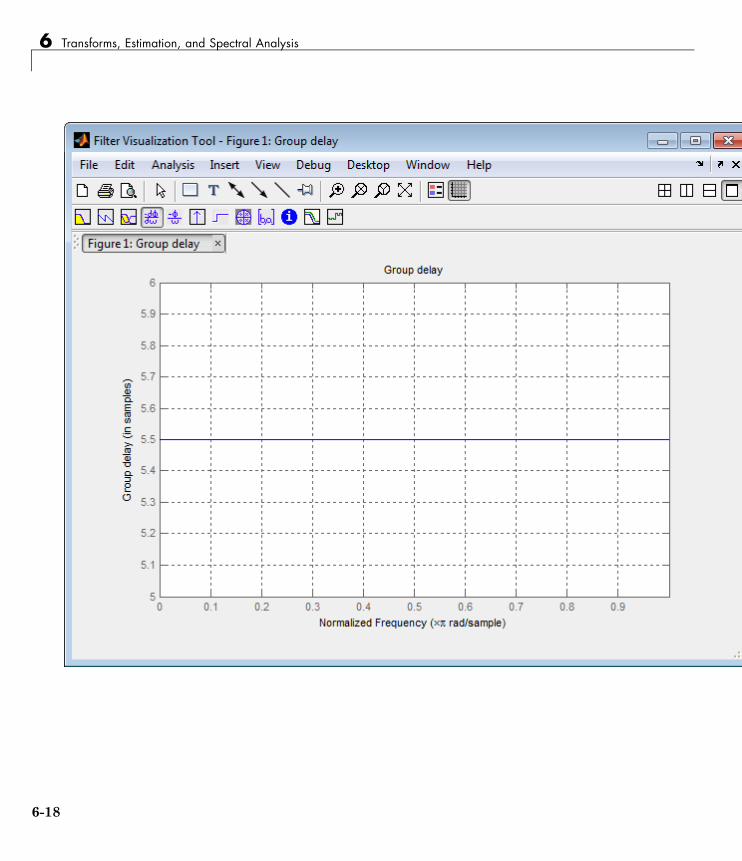
6 Transforms, Estimation, and Spectral Analysis
6-18

Calculate Channel Latencies Required for Wavelet Reconstruction
Note Repeat this procedure to analyze the group delay of each of the filtersin your model. This section does not show the results for each filter in theex_wavelets model because all wavelet filters in this particular examplehave the same group delay.
Reconstruct the Filter Bank SystemTo determine the delay introduced by the analysis and synthesis filter banksystem, you must reconstruct the tree structures of the Dyadic Analysis FilterBank and the Dyadic Synthesis Filter Bank blocks. To learn more aboutconstructing tree structures for the Dyadic Analysis Filter Bank and DyadicSynthesis Filter Bank blocks, see the following sections of the DSP SystemToolbox User’s Guide:
• “Dyadic Analysis Filter Banks” on page 5-12
• “Dyadic Synthesis Filter Banks” on page 5-16
Because the filter blocks in the ex_wavelets model use biorthogonal filterswith three levels and an asymmetric tree structure, the filter bank systemappears as shown in the following figure.
F0
F0
F0
F1
F0
F0
F12
2
2
2
2
2 F0
F1 2
2
2
2
2
G1
G0
G0
G0 G0
G02
2
2
2
22
2
G1
G1
G0Delay M
Delay N
Path 1
Path 2
Path 3
Path 4
F0 = Delay due to low-pass filter of Dyadic Analysis Filter BankF1 = Delay due to high-pass filter of Dyadic Analysis Filter BankG0 = Delay due to low-pass filter of Dyadic Synthesis Filter BankG1 = Delay due to high-pass filter of Dyadic Synthesis Filter Bank
6-19
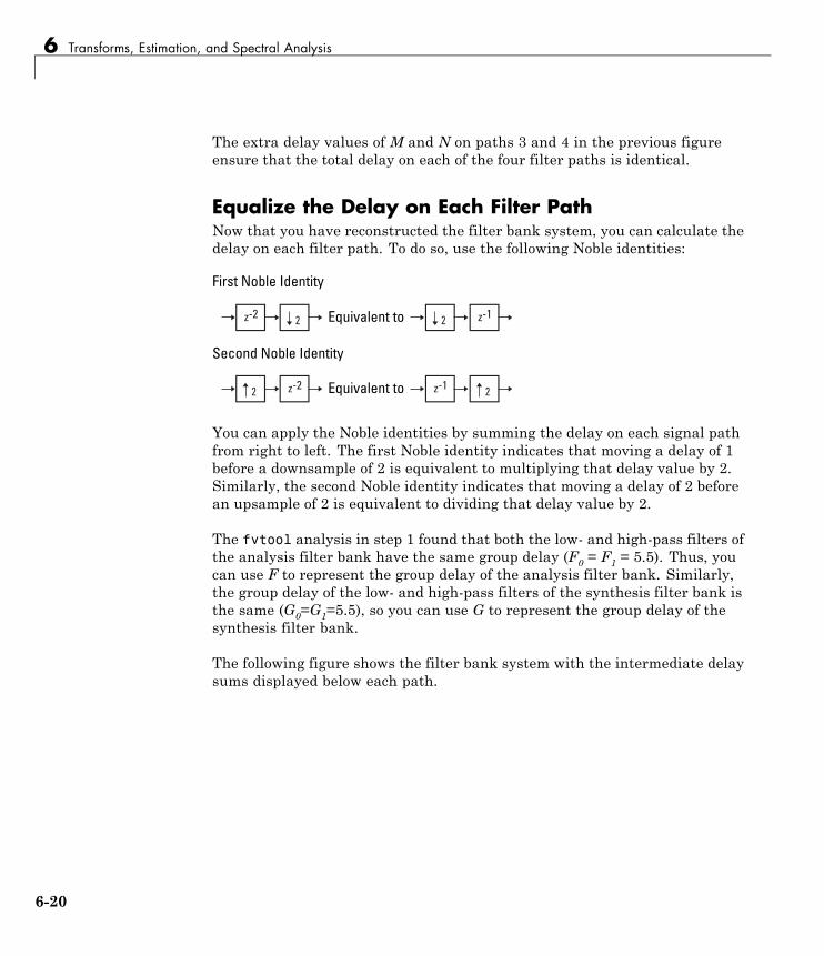
6 Transforms, Estimation, and Spectral Analysis
The extra delay values of M and N on paths 3 and 4 in the previous figureensure that the total delay on each of the four filter paths is identical.
Equalize the Delay on Each Filter PathNow that you have reconstructed the filter bank system, you can calculate thedelay on each filter path. To do so, use the following Noble identities:
2
2 z-2 z-1 2
2 z-1z-2
Equivalent to
Equivalent to
Second Noble Identity
First Noble Identity
You can apply the Noble identities by summing the delay on each signal pathfrom right to left. The first Noble identity indicates that moving a delay of 1before a downsample of 2 is equivalent to multiplying that delay value by 2.Similarly, the second Noble identity indicates that moving a delay of 2 beforean upsample of 2 is equivalent to dividing that delay value by 2.
The fvtool analysis in step 1 found that both the low- and high-pass filters ofthe analysis filter bank have the same group delay (F0 = F1 = 5.5). Thus, youcan use F to represent the group delay of the analysis filter bank. Similarly,the group delay of the low- and high-pass filters of the synthesis filter bank isthe same (G0=G1=5.5), so you can use G to represent the group delay of thesynthesis filter bank.
The following figure shows the filter bank system with the intermediate delaysums displayed below each path.
6-20

Calculate Channel Latencies Required for Wavelet Reconstruction
F
F
F
F
F
F
F2
2
2
2
2
2 F
F 2
2
2
2
2
G
G
G
G G
G2
2
2
2
22
2
G
G
GDelay M
Delay N
Path 1
Path 2
Path 3
Path 4
G0.5GN+0.5G2N+G2N+(F+G)
G
G
G
0.5G
0.5G
0.5G
1.5G
1.5G
1.5G
0.75G
0.75G
0.75G
1.75G
1.75G
0.875G
0.875G
1.75G
1.75G
F+1.75G
F+1.75G
2F+3.5G
2F+3.5G
3F+3.5G
3F+3.5G
6F+7G
6F+7G
7(F+G)
7(F+G)
M+0.75G2M+1.5G2M+F+1.5G4M+2F+3G4M+3(F+G)
F = Delay due to Dyadic Analysis Filter BankG = Delay due to Dyadic Synthesis Filter Bank
You can see from the previous figure that the signal delays on paths 1 and2 are identical: 7(F+G). Because each path of the filter bank system hasidentical delay, you can equate the delay equations for paths 3 and 4 with thedelay equation for paths 1 and 2. After constructing these equations, youcan solve for M and N, respectively:
Path 3 = Path 1
⇒ + + = +4 3 7M F G F G( ) ( )⇒⇒ = +
⇒ + + = +
M F G
N F G F GPath 4 = Path 1
2 7( ) ( ) ⇒ = +N F G3( )
The fvtool analysis in step 1 found the group delay of each biorthogonalwavelet filter in this model to be 5.5 samples. Therefore, F = 5.5 and G =5.5. By inserting these values into the two previous equations, you get M =11 and N = 33. Because the total delay on each filter path must be the same,you can find the overall delay of the filter bank system by inserting F = 5.5
6-21

6 Transforms, Estimation, and Spectral Analysis
and G = 5.5 into the delay equation for any of the four filter paths. Insertingthe values of F and G into 7(F+G) yields an overall delay of 77 samples forthe filter bank system of the ex_wavelets model.
Update and Run the ModelNow that you know the latencies required for perfect wavelet reconstruction,you can incorporate those delay values into the model. The ex_waveletsmodel has already been updated with the correct delay values (M = 11, N =33, Overall = 77), so it is ready to run.
After you run the model, examine the reconstruction error in the Differencescope. To further examine any particular areas of interest, use the zoom toolsavailable on the toolbar of the scope window or from the View menu.
6-22
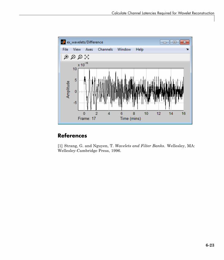
Calculate Channel Latencies Required for Wavelet Reconstruction
References
[1] Strang, G. and Nguyen, T. Wavelets and Filter Banks. Wellesley, MA:Wellesley-Cambridge Press, 1996.
6-23

6 Transforms, Estimation, and Spectral Analysis
Spectral AnalysisThe Power Spectrum Estimation library provides a number of blocks forspectral analysis. Many of them have correlates in Signal Processing Toolboxsoftware, which are shown in parentheses:
• Burg Method (pburg)
• Covariance Method (pcov)
• Magnitude FFT (periodogram)
• Modified Covariance Method (pmcov)
• Short-Time FFT
• Yule-Walker Method (pyulear)
See “Spectral Analysis” in the Signal Processing Toolbox documentation foran overview of spectral analysis theory and a discussion of the above methods.
DSP System Toolbox software provides two examples that illustrate thespectral analysis blocks:
• A Comparison of Spectral Analysis Techniques (dspsacomp)
• Spectral Analysis: Short-Time FFT (dspstfft)
6-24

Power Spectrum Estimates
Power Spectrum Estimates
In this section...
“Create the Block Diagram” on page 6-25
“Set the Model Parameters” on page 6-26
“View the Power Spectrum Estimates” on page 6-33
Create the Block DiagramUp until now, you have been dealing with signals in the time domain. TheDSP System Toolbox product is also capable of working with signals inthe frequency domain. You can use the software to perform fast Fouriertransforms (FFTs), power spectrum analysis, short-time FFTs, and manyother frequency-domain applications.
The power spectrum of a signal represents the contribution of every frequencyof the spectrum to the power of the overall signal. It is useful becausemany signal processing applications, such as noise cancellation and systemidentification, are based on frequency-specific modifications of signals.
First, assemble and connect the blocks needed to calculate the power spectrumof your speech signal:
1 Open a new Simulink model.
2 Add the following blocks to your model. Subsequent topics describe howto use these blocks.
Block Library
Signal From Workspace Sources
Buffer Signal Management / Buffers
Periodogram Estimation / Power SpectrumEstimation
Vector Scope Sinks
3 Connect the blocks as shown in the next figure.
6-25
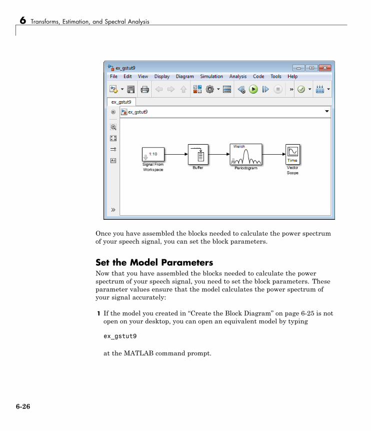
6 Transforms, Estimation, and Spectral Analysis
Once you have assembled the blocks needed to calculate the power spectrumof your speech signal, you can set the block parameters.
Set the Model ParametersNow that you have assembled the blocks needed to calculate the powerspectrum of your speech signal, you need to set the block parameters. Theseparameter values ensure that the model calculates the power spectrum ofyour signal accurately:
1 If the model you created in “Create the Block Diagram” on page 6-25 is notopen on your desktop, you can open an equivalent model by typing
ex_gstut9
at the MATLAB command prompt.
6-26

Power Spectrum Estimates
2 Load the speech signal into the MATLAB workspace by typing load mtlbat the MATLAB command prompt. This speech signal is a woman’s voicesaying “MATLAB.”
3 Use the Signal From Workspace block to import the speech signal fromthe MATLAB workspace into your Simulink model. Open the SignalFrom Workspace dialog box by double-clicking the block. Set the blockparameters as follows:
• Signal = mtlb
• Sample time = 1/8000
• Samples per frame = 80
• Form output after final data value by = Setting to zero
Once you are done setting these parameters, the Signal From Workspacedialog box should look similar to the figure below. Click OK to apply yourchanges.
6-27
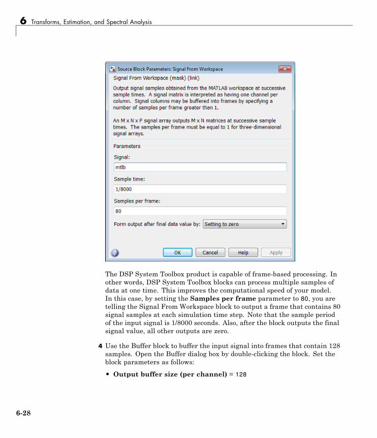
6 Transforms, Estimation, and Spectral Analysis
The DSP System Toolbox product is capable of frame-based processing. Inother words, DSP System Toolbox blocks can process multiple samples ofdata at one time. This improves the computational speed of your model.In this case, by setting the Samples per frame parameter to 80, you aretelling the Signal From Workspace block to output a frame that contains 80signal samples at each simulation time step. Note that the sample periodof the input signal is 1/8000 seconds. Also, after the block outputs the finalsignal value, all other outputs are zero.
4 Use the Buffer block to buffer the input signal into frames that contain 128samples. Open the Buffer dialog box by double-clicking the block. Set theblock parameters as follows:
• Output buffer size (per channel) = 128
6-28
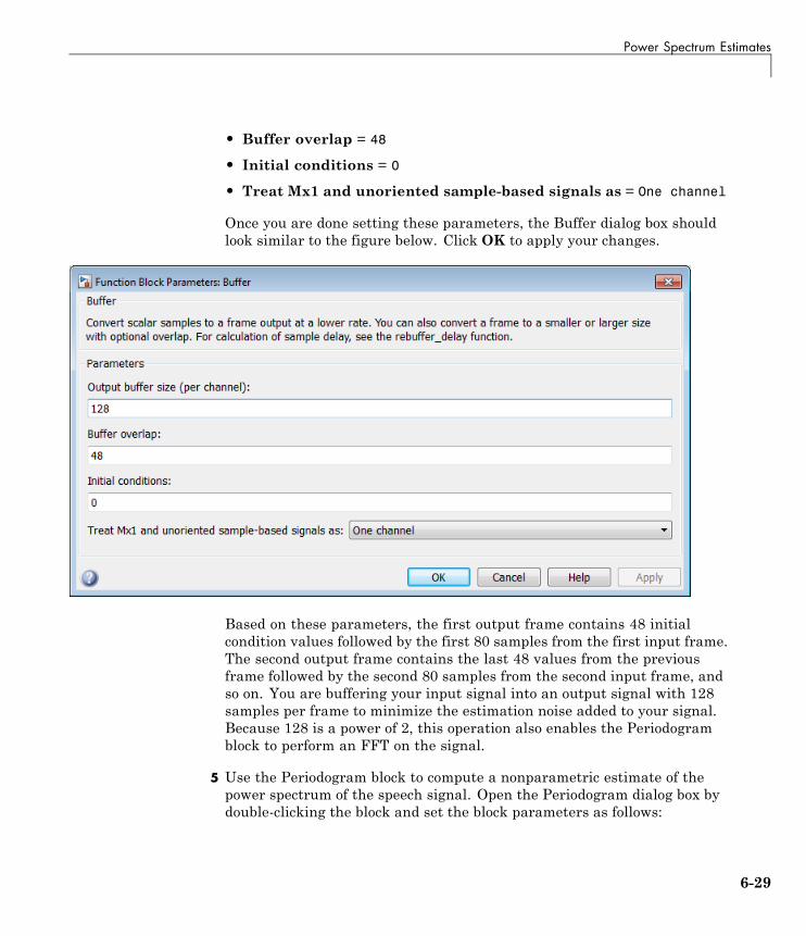
Power Spectrum Estimates
• Buffer overlap = 48
• Initial conditions = 0
• Treat Mx1 and unoriented sample-based signals as = One channel
Once you are done setting these parameters, the Buffer dialog box shouldlook similar to the figure below. Click OK to apply your changes.
Based on these parameters, the first output frame contains 48 initialcondition values followed by the first 80 samples from the first input frame.The second output frame contains the last 48 values from the previousframe followed by the second 80 samples from the second input frame, andso on. You are buffering your input signal into an output signal with 128samples per frame to minimize the estimation noise added to your signal.Because 128 is a power of 2, this operation also enables the Periodogramblock to perform an FFT on the signal.
5 Use the Periodogram block to compute a nonparametric estimate of thepower spectrum of the speech signal. Open the Periodogram dialog box bydouble-clicking the block and set the block parameters as follows:
6-29
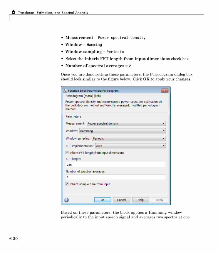
6 Transforms, Estimation, and Spectral Analysis
• Measurement = Power spectral density
• Window = Hamming
• Window sampling = Periodic
• Select the Inherit FFT length from input dimensions check box.
• Number of spectral averages = 2
Once you are done setting these parameters, the Periodogram dialog boxshould look similar to the figure below. Click OK to apply your changes.
Based on these parameters, the block applies a Hamming windowperiodically to the input speech signal and averages two spectra at one
6-30

Power Spectrum Estimates
time. The length of the FFT is assumed to be 128, which is the number ofsamples per frame being output from the Buffer block.
6 Use the Vector Scope block to view the power spectrum of the speech signal.Open the Vector Scope dialog box by double-clicking the block. Set theblock parameters as follows:
• Input domain = Frequency
• Click the Axis Properties tab.
• Clear the Inherit sample time from input check box.
• Sample time of original time series = 1/8000
• Y-axis label = Magnitude-squared, dB
Once you are done setting these parameters, the Axis Properties paneof the Vector Scope dialog box should look similar to the figure below. Asyou can see by the Y-axis scaling parameter, the decibel amplitude isplotted in a vector scope window.
6-31
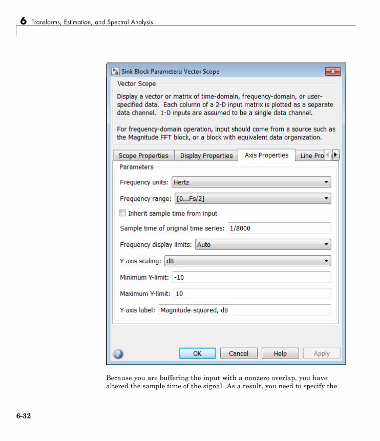
6 Transforms, Estimation, and Spectral Analysis
Because you are buffering the input with a nonzero overlap, you havealtered the sample time of the signal. As a result, you need to specify the
6-32

Power Spectrum Estimates
sample time of the original time series. Otherwise, the overlapping buffersamples lead the block to believe that the sample time is shorter than itactually is.
After you have set the block parameter values, you can calculate and view thepower spectrum of the speech signal.
View the Power Spectrum EstimatesIn the previous topics, you created a power spectrum model and set itsparameters. In this topic, you simulate the model and view the powerspectrum of your speech signal:
1 If the model you created in “Set the Model Parameters” on page 6-26 is notopen on your desktop, you can open an equivalent model by typing
ex_gstut10
at the MATLAB command prompt.
2 Set the configuration parameters. Open the Configuration Parametersdialog box by selecting Model Configuration Parameters from theSimulation menu. Select Solver from the menu on the left side of thedialog box, and set the parameters as follows:
• Stop time = 0.5
• Type = Fixed-step
• Solver = Discrete (no continuous states)
6-33

6 Transforms, Estimation, and Spectral Analysis
3 Apply these parameters and close the Configuration Parameters dialogbox by clicking OK. These parameters are saved only when you save yourmodel.
4 If you have not already done so, load the speech signal into the MATLABworkspace by typing load mtlb.
5 Run the model to open the Vector Scope window. The data is notimmediately visible at the end of the simulation. To autoscale the y-axis tofit the data, in the Vector Scope window, right-click and choose Autoscale.The following figure shows the data displayed in the Vector Scope window.
6-34

Power Spectrum Estimates
During the simulation, the Vector Scope window displays a series of framesoutput from the Periodogram block. Each of these frames corresponds toa window of the original speech signal. The data in each frame representsthe power spectrum, or contribution of every frequency to the power of theoriginal speech signal, for a given window.
In the next section, “Spectrograms” on page 6-36, you use these power spectrato create a spectrogram of the speech signal.
6-35
6 Transforms, Estimation, and Spectral Analysis
Spectrograms
In this section...
“Modify the Block Diagram” on page 6-36
“Set the Model Parameters” on page 6-38
“View the Spectrogram of the Speech Signal” on page 6-43
Modify the Block DiagramSpectrograms are color-based visualizations of the evolution of thepower spectrum of a speech signal as this signal is swept through time.Spectrograms use the periodogram power spectrum estimation method andare widely used by speech and audio engineers. You can use them to developa visual understanding of the frequency content of your speech signal while aparticular sound is being vocalized.
In the previous section, you built a model capable of calculating the powerspectrum of a speech signal that represents a woman saying “MATLAB.” Inthis topic, you modify this model to view the spectrogram of your signal:
1 If the model you created in “View the Power Spectrum Estimates” onpage 6-33 is not open on your desktop, you can open an equivalent modelby typing
ex_gstut11
at the MATLAB command prompt.
6-36
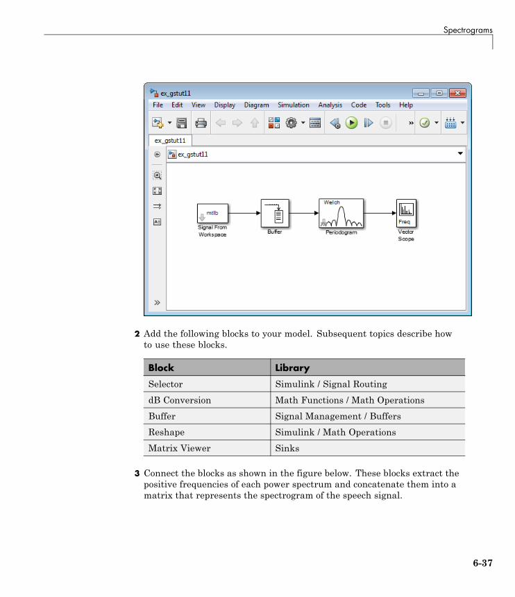
Spectrograms
2 Add the following blocks to your model. Subsequent topics describe howto use these blocks.
Block Library
Selector Simulink / Signal Routing
dB Conversion Math Functions / Math Operations
Buffer Signal Management / Buffers
Reshape Simulink / Math Operations
Matrix Viewer Sinks
3 Connect the blocks as shown in the figure below. These blocks extract thepositive frequencies of each power spectrum and concatenate them into amatrix that represents the spectrogram of the speech signal.
6-37
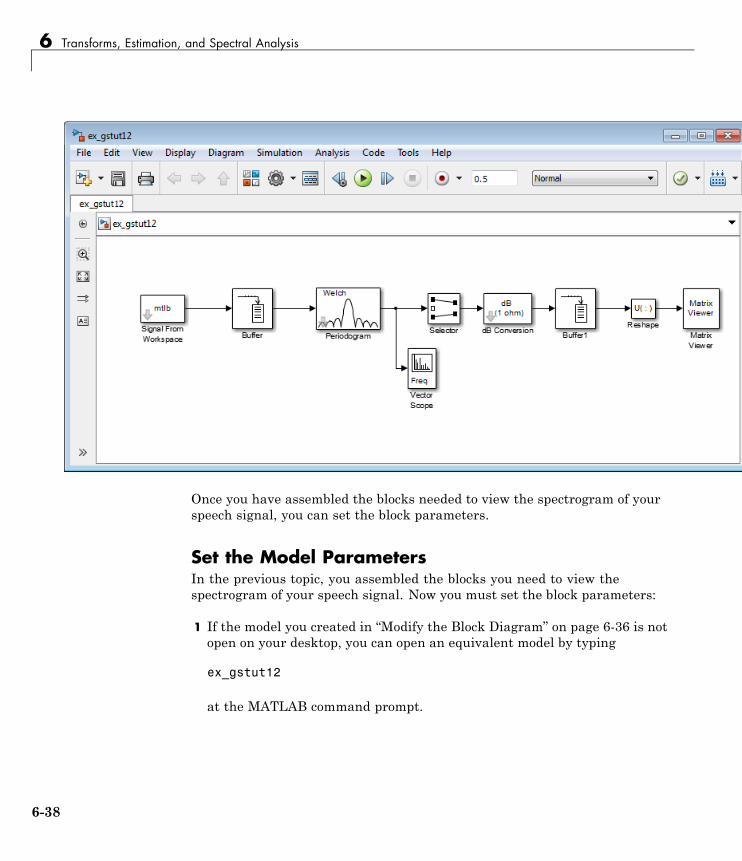
6 Transforms, Estimation, and Spectral Analysis
Once you have assembled the blocks needed to view the spectrogram of yourspeech signal, you can set the block parameters.
Set the Model ParametersIn the previous topic, you assembled the blocks you need to view thespectrogram of your speech signal. Now you must set the block parameters:
1 If the model you created in “Modify the Block Diagram” on page 6-36 is notopen on your desktop, you can open an equivalent model by typing
ex_gstut12
at the MATLAB command prompt.
6-38

Spectrograms
2 Use the Selector block to extract the first 64 elements, or the positivefrequencies, of each power spectrum. Open the Selector dialog box bydouble-clicking the block. Set the block parameters as follows:
• Number of input dimensions = 1
• Index mode = One-based
• Index option = Index vector (dialog)
• Index = 1:64
• Input port size = 128
At each time instance, the input to the Selector block is a vector of 128elements. The block assigns one-based indices to these elements andextracts the first 64. Once you are done setting these parameters, theSelector dialog box should look similar to the figure below. To apply yourchanges, click OK.
6-39

6 Transforms, Estimation, and Spectral Analysis
3 The dB Conversion block converts the magnitude of the input FFT signal todecibels. Leave this block at its default parameters.
4 Use the Buffer1 block to buffer up the individual power spectrums.Open the Buffer1 dialog box by double-clicking the block. Set the blockparameters as follows:
• Output buffer size (per channel) = 64*48
• Buffer overlap = 64*46
• Initial conditions = -70
• Treat Mx1 and unoriented sample-based signals as = One channel
Once you are done setting these parameters, the Buffer1 dialog box shouldlook similar to the following figure. To apply your changes, click OK.
Setting the value of the Buffer overlap parameter slightly less thanthe value of the Output buffer size (per channel) parameter ensuresthat your spectrogram represents smooth movement through time. The
6-40

Spectrograms
Initial conditions parameter represents the initial values in the buffer;-70 represents silence.
5 Use the Reshape block to reshape the input signal into a 64-by-48 matrix.To do so, set the Output dimensionality to Customize and the Outputdimensions to [64 48].
6 The Matrix Viewer enables you to view the spectrogram of the speechsignal. Open the Matrix Viewer dialog box by double-clicking the block.Set the block parameters as follows:
• Click the Image Properties tab.
• Colormap matrix = jet(256)
• Minimum input value = -150
• Maximum input value = -65
• Select the Display colorbar check box.
Once you are done setting these parameters, the Image Properties paneshould look similar to the figure below.
6-41
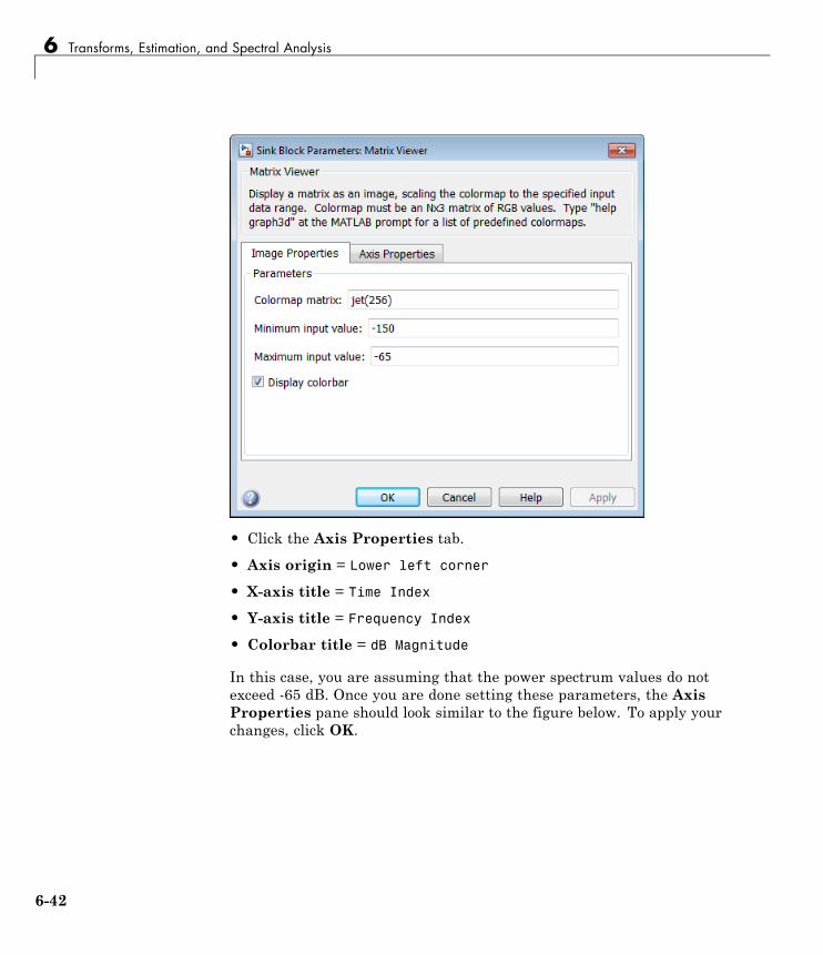
6 Transforms, Estimation, and Spectral Analysis
• Click the Axis Properties tab.
• Axis origin = Lower left corner
• X-axis title = Time Index
• Y-axis title = Frequency Index
• Colorbar title = dB Magnitude
In this case, you are assuming that the power spectrum values do notexceed -65 dB. Once you are done setting these parameters, the AxisProperties pane should look similar to the figure below. To apply yourchanges, click OK.
6-42

Spectrograms
After you have set the parameter values, you can calculate and view thespectrogram of the speech signal.
View the Spectrogram of the Speech SignalIn the topic “View the Power Spectrum Estimates” on page 6-33, you used aVector Scope block to display the power spectrum of your speech signal. In thistopic, you view the spectrogram of your speech signal using a Matrix Viewerblock. The speech signal represents a woman’s voice saying “MATLAB”:
1 If the model you created in “Set the Model Parameters” on page 6-38 is notopen on your desktop, you can open an equivalent model by typing
ex_gstut13
at the MATLAB command prompt.
6-43

6 Transforms, Estimation, and Spectral Analysis
2 Run the model. During the simulation, the Vector Scope window displays asequence of power spectrums, one for each window of the original speechsignal. The power spectrum is the contribution of every frequency to thepower of the speech signal.
6-44

Spectrograms
The Matrix Viewer window, shown below, displays the spectrogram ofthe speech signal. This spectrogram is calculated using the Periodogrampower spectrum estimation method. Note the harmonics that are visiblein the signal when the vowels are spoken. Most of the signal’s energy isconcentrated in these harmonics; therefore, two distinct peaks are visiblein the spectrogram.
6-45

6 Transforms, Estimation, and Spectral Analysis
In this example, you viewed the spectrogram of your speech signal using aMatrix Viewer block. You can find additional DSP System Toolbox productexamples in the Help browser. To access these examples, click the Contentstab, double-click DSP System Toolbox, and then click Examples. A list ofthe examples in the DSP System Toolbox documentation appears in the rightpane of the Help browser.
6-46

7
Mathematics
Learn about statistics and linear algebra.
• “Statistics” on page 7-2
• “Linear Algebra and Least Squares” on page 7-6

7 Mathematics
Statistics
In this section...
“Statistics Blocks” on page 7-2
“Basic Operations” on page 7-3
“Running Operations” on page 7-4
Statistics BlocksThe Statistics library provides fundamental statistical operations such asminimum, maximum, mean, variance, and standard deviation. Most blocks inthe Statistics library support two types of operations; basic and running.
The blocks listed below toggle between basic and running modes using theRunning check box in the parameter dialog box:
• Histogram
• Mean
• RMS
• Standard Deviation
• Variance
An unselected Running check box means that the block is operating inbasic mode, while a selected Running box means that the block is operatingin running mode.
The Maximum and Minimum blocks are slightly different from the blocksabove, and provide a Mode parameter in the block dialog box to select thetype of operation. The Value and Index, Value, and Index options in theMode menu all specify basic operation, in each case enabling a different setof output ports on the block. The Running option in the Mode menu selectsrunning operation.
7-2

Statistics
Basic OperationsA basic operation is one that processes each input independently of previousand subsequent inputs. For example, in basic mode (with Value and Indexselected, for example) the Maximum block finds the maximum value in eachcolumn of the current input, and returns this result at the top output (Val).Each consecutive Val output therefore has the same number of columns asthe input, but only one row. Furthermore, the values in a given output onlydepend on the values in the corresponding input. The block repeats thisoperation for each successive input.
This type of operation is exactly equivalent to the MATLAB command
val = max(u) % Equivalent MATLAB code
which computes the maximum of each column in input u.
The next section is an example of a basic statistical operation.
Create a Sliding WindowYou can use the basic statistics operations in conjunction with the Bufferblock to implement basic sliding window statistics operations. A slidingwindow is like a stencil that you move along a data stream, exposing only aset number of data points at one time.
For example, you may want to process data in 128-sample frames, moving thewindow along by one sample point for each operation. One way to implementsuch a sliding window is shown in the following ex_mean_tut model.
The Buffer block’s Buffer size (Mo) parameter determines the size of thewindow. The Buffer overlap (L) parameter defines the “slide factor” forthe window. At each sample instant, the window slides by Mo-L points. TheBuffer overlap is often Mo-1, so that a new statistic is computed for everynew signal sample.
7-3
7 Mathematics
Running OperationsA running operation is one that processes successive inputs, and computesa result that reflects both current and past inputs. In this mode, you mustuse the Input processing parameter to specify whether the block performssample- or frame-based processing on the inputs. A reset port enables youto restart this tracking at any time. The running statistic is computed foreach input channel independently, so the block’s output is the same size asthe input.
For example, in running mode (Running selected from the Mode parameter)the Maximum block outputs a record of the input’s maximum value over time.
7-4
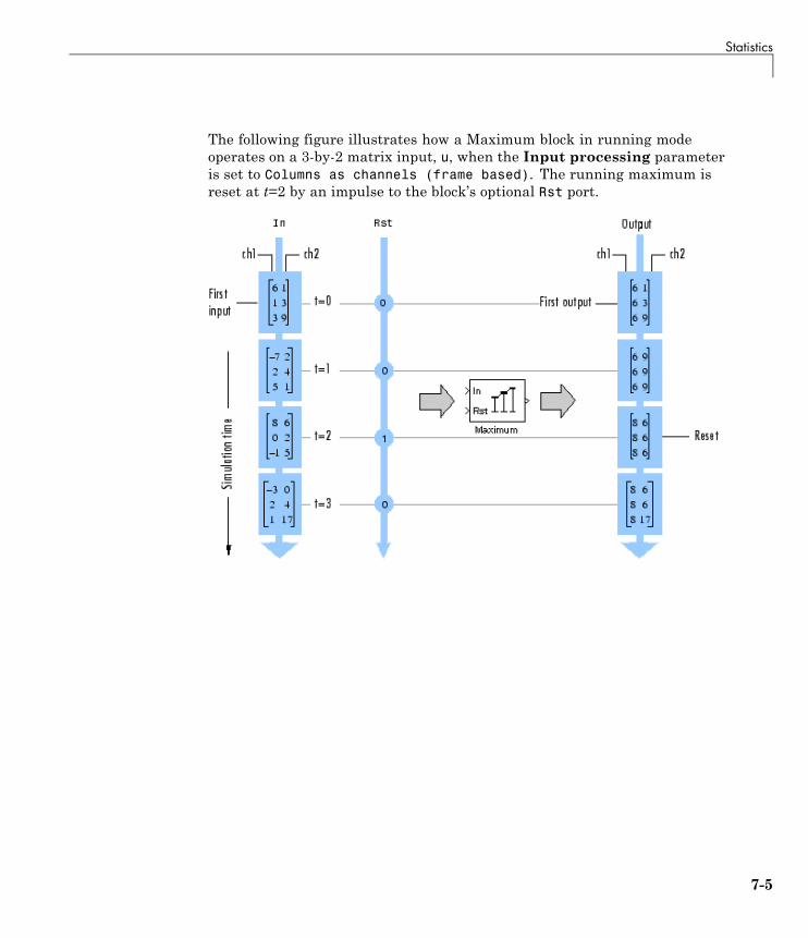
Statistics
The following figure illustrates how a Maximum block in running modeoperates on a 3-by-2 matrix input, u, when the Input processing parameteris set to Columns as channels (frame based). The running maximum isreset at t=2 by an impulse to the block’s optional Rst port.
7-5

7 Mathematics
Linear Algebra and Least Squares
In this section...
“Linear Algebra Blocks” on page 7-6
“Linear System Solvers” on page 7-6
“Matrix Factorizations” on page 7-8
“Matrix Inverses” on page 7-9
Linear Algebra BlocksThe Matrices and Linear Algebra library provides three large sublibrariescontaining blocks for linear algebra; Linear System Solvers, MatrixFactorizations, and Matrix Inverses. A fourth library, Matrix Operations,provides other essential blocks for working with matrices.
Linear System SolversThe Linear System Solvers library provides the following blocks for solvingthe system of linear equations AX = B:
• Autocorrelation LPC
• Cholesky Solver
• Forward Substitution
• LDL Solver
• Levinson-Durbin
• LU Solver
• QR Solver
• SVD Solver
Some of the blocks offer particular strengths for certain classes of problems.For example, the Cholesky Solver block is particularly adapted for a squareHermitian positive definite matrix A, whereas the Backward Substitutionblock is particularly suited for an upper triangular matrix A.
7-6
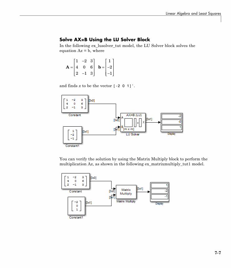
Linear Algebra and Least Squares
Solve AX=B Using the LU Solver BlockIn the following ex_lusolver_tut model, the LU Solver block solves theequation Ax = b, where
A b=−
−
⎡
⎣
⎢⎢⎢
⎤
⎦
⎥⎥⎥
= −−
⎡
⎣
⎢⎢⎢
⎤
⎦
⎥⎥⎥
1 2 34 0 62 1 3
121
and finds x to be the vector [-2 0 1]'.
You can verify the solution by using the Matrix Multiply block to perform themultiplication Ax, as shown in the following ex_matrixmultiply_tut1 model.
7-7

7 Mathematics
Matrix FactorizationsThe Matrix Factorizations library provides the following blocks for factoringvarious kinds of matrices:
• Cholesky Factorization
• LDL Factorization
• LU Factorization
• QR Factorization
• Singular Value Decomposition
Some of the blocks offer particular strengths for certain classes of problems.For example, the Cholesky Factorization block is particularly suited tofactoring a Hermitian positive definite matrix into triangular components,whereas the QR Factorization is particularly suited to factoring a rectangularmatrix into unitary and upper triangular components.
Factor a Matrix into Upper and Lower Submatrices Using theLU Factorization BlockIn the following ex_lufactorization_tut model, the LU Factorization blockfactors a matrix Ap into upper and lower triangular submatrices U and L,where Ap is row equivalent to input matrix A, where
7-8

Linear Algebra and Least Squares
The lower output of the LU Factorization, P, is the permutation indexvector, which indicates that the factored matrix Ap is generated from A byinterchanging the first and second rows.
A p = −−
⎡
⎣
⎢⎢⎢
⎤
⎦
⎥⎥⎥
4 0 61 2 32 1 3
The upper output of the LU Factorization, LU, is a composite matrix containingthe two submatrix factors, U and L, whose product LU is equal to Ap.
U L= −−
⎡
⎣
⎢⎢⎢
⎤
⎦
⎥⎥⎥
=⎡
⎣
⎢⎢⎢
⎤
⎦
⎥⎥⎥
4 0 60 2 1 50 0 0 75
1 0 00 25 1 00 5 0 5 1
.
... .
You can check that LU = Ap with the Matrix Multiply block, as shown in thefollowing ex_matrixmultiply_tut2 model.
Matrix InversesThe Matrix Inverses library provides the following blocks for inverting variouskinds of matrices:
• Cholesky Inverse
• LDL Inverse
7-9

7 Mathematics
• LU Inverse
• Pseudoinverse
Find the Inverse of a Matrix Using the LU Inverse BlockIn the following ex_luinverse_tut model, the LU Inverse block computes theinverse of input matrix A, where
A =−
−
⎡
⎣
⎢⎢⎢
⎤
⎦
⎥⎥⎥
1 2 34 0 62 1 3
and then forms the product A-1A, which yields the identity matrix of order 3,as expected.
As shown above, the computed inverse is
A− =− −
−−
⎡
⎣
⎢⎢⎢
⎤
⎦
⎥⎥⎥
11 0 5 2
0 0 5 10 6667 0 5 1 333
..
. . .
7-10

8
Fixed-Point Design
Learn about fixed-point data types and how to convert floating-point modelsto fixed-point.
• “Fixed-Point Signal Processing” on page 8-2
• “Fixed-Point Concepts and Terminology” on page 8-4
• “Arithmetic Operations” on page 8-10
• “Fixed-Point Support for MATLAB System Objects” on page 8-21
• “Specify Fixed-Point Attributes for Blocks” on page 8-28
• “Quantizers” on page 8-52
• “Fixed-Point Filter Design” on page 8-68
8 Fixed-Point Design
Fixed-Point Signal Processing
In this section...
“Fixed-Point Features” on page 8-2
“Benefits of Fixed-Point Hardware” on page 8-2
“Benefits of Fixed-Point Design with System Toolboxes Software” on page8-3
Note To take full advantage of fixed-point support in System Toolboxsoftware, you must install Fixed-Point Designer software.
Fixed-Point FeaturesMany of the blocks in this product have fixed-point support, so you can designsignal processing systems that use fixed-point arithmetic. Fixed-point supportin DSP System Toolbox software includes
• Signed two’s complement and unsigned fixed-point data types
• Word lengths from 2 to 128 bits in simulation
• Word lengths from 2 to the size of a long on the Simulink Coder Ccode-generation target
• Overflow handling and rounding methods
• C code generation for deployment on a fixed-point embedded processor,with Simulink Coder code generation software. The generated code uses allallowed data types supported by the embedded target, and automaticallyincludes all necessary shift and scaling operations
Benefits of Fixed-Point HardwareThere are both benefits and trade-offs to using fixed-point hardware ratherthan floating-point hardware for signal processing development. Many signalprocessing applications require low-power and cost-effective circuitry, whichmakes fixed-point hardware a natural choice. Fixed-point hardware tends tobe simpler and smaller. As a result, these units require less power and costless to produce than floating-point circuitry.
8-2

Fixed-Point Signal Processing
Floating-point hardware is usually larger because it demands functionalityand ease of development. Floating-point hardware can accurately representreal-world numbers, and its large dynamic range reduces the risk of overflow,quantization errors, and the need for scaling. In contrast, the smaller dynamicrange of fixed-point hardware that allows for low-power, inexpensive unitsbrings the possibility of these problems. Therefore, fixed-point developmentmust minimize the negative effects of these factors, while exploiting thebenefits of fixed-point hardware; cost- and size-effective units, less power andmemory usage, and fast real-time processing.
Benefits of Fixed-Point Design with System ToolboxesSoftwareSimulating your fixed-point development choices before implementing themin hardware saves time and money. The built-in fixed-point operationsprovided by the System Toolboxes software save time in simulation and allowyou to generate code automatically.
This software allows you to easily run multiple simulations with differentword length, scaling, overflow handling, and rounding method choices tosee the consequences of various fixed-point designs before committingto hardware. The traditional risks of fixed-point development, such asquantization errors and overflow, can be simulated and mitigated in softwarebefore going to hardware.
Fixed-point C code generation with System Toolbox software and SimulinkCoder code generation software produces code ready for execution on afixed-point processor. All the choices you make in simulation in termsof scaling, overflow handling, and rounding methods are automaticallyoptimized in the generated code, without necessitating time-consuming andcostly hand-optimized code.
8-3
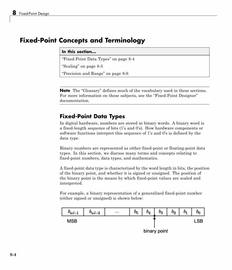
8 Fixed-Point Design
Fixed-Point Concepts and Terminology
In this section...
“Fixed-Point Data Types” on page 8-4
“Scaling” on page 8-5
“Precision and Range” on page 8-6
Note The “Glossary” defines much of the vocabulary used in these sections.For more information on these subjects, see the “Fixed-Point Designer”documentation.
Fixed-Point Data TypesIn digital hardware, numbers are stored in binary words. A binary word isa fixed-length sequence of bits (1’s and 0’s). How hardware components orsoftware functions interpret this sequence of 1’s and 0’s is defined by thedata type.
Binary numbers are represented as either fixed-point or floating-point datatypes. In this section, we discuss many terms and concepts relating tofixed-point numbers, data types, and mathematics.
A fixed-point data type is characterized by the word length in bits, the positionof the binary point, and whether it is signed or unsigned. The position ofthe binary point is the means by which fixed-point values are scaled andinterpreted.
For example, a binary representation of a generalized fixed-point number(either signed or unsigned) is shown below:
8-4
Fixed-Point Concepts and Terminology
where
• bi is the ith binary digit.
• wl is the word length in bits.
• bwl–1 is the location of the most significant, or highest, bit (MSB).
• b0 is the location of the least significant, or lowest, bit (LSB).
• The binary point is shown four places to the left of the LSB. In thisexample, therefore, the number is said to have four fractional bits, or afraction length of four.
Fixed-point data types can be either signed or unsigned. Signed binaryfixed-point numbers are typically represented in one of three ways:
• Sign/magnitude
• One’s complement
• Two’s complement
Two’s complement is the most common representation of signed fixed-pointnumbers and is used by System Toolbox software. See “Two’s Complement”on page 8-11 for more information.
ScalingFixed-point numbers can be encoded according to the scheme
real world value slope integer bias- ( )
where the slope can be expressed as
slope slope adjustment exponent 2
The integer is sometimes called the stored integer. This is the raw binarynumber, in which the binary point assumed to be at the far right of the word.In System Toolboxes, the negative of the exponent is often referred to asthe fraction length.
8-5

8 Fixed-Point Design
The slope and bias together represent the scaling of the fixed-point number.In a number with zero bias, only the slope affects the scaling. A fixed-pointnumber that is only scaled by binary point position is equivalent to a numberin the Fixed-Point Designer [Slope Bias] representation that has a bias equalto zero and a slope adjustment equal to one. This is referred to as binarypoint-only scaling or power-of-two scaling:
real world value integerexponent- 2
or
real world value integerfraction length- 2
In System Toolbox software, you can define a fixed-point data type and scalingfor the output or the parameters of many blocks by specifying the word lengthand fraction length of the quantity. The word length and fraction lengthdefine the whole of the data type and scaling information for binary-pointonly signals.
All System Toolbox blocks that support fixed-point data types support signalswith binary-point only scaling. Many fixed-point blocks that do not performarithmetic operations but merely rearrange data, such as Delay and MatrixTranspose, also support signals with [Slope Bias] scaling.
Precision and RangeYou must pay attention to the precision and range of the fixed-point datatypes and scalings you choose for the blocks in your simulations, in order toknow whether rounding methods will be invoked or if overflows will occur.
RangeThe range is the span of numbers that a fixed-point data type and scalingcan represent. The range of representable numbers for a two’s complementfixed-point number of word length wl, scaling S, and bias B is illustratedbelow:
8-6

Fixed-Point Concepts and Terminology
For both signed and unsigned fixed-point numbers of any data type, thenumber of different bit patterns is 2wl.
For example, in two’s complement, negative numbers must be representedas well as zero, so the maximum value is 2wl–1. Because there is only onerepresentation for zero, there are an unequal number of positive and negativenumbers. This means there is a representation for -2wl–1 but not for 2wl –1:
Overflow Handling. Because a fixed-point data type represents numberswithin a finite range, overflows can occur if the result of an operation is largeror smaller than the numbers in that range.
System Toolbox software does not allow you to add guard bits to a data typeon-the-fly in order to avoid overflows. Any guard bits must be allocatedupon model initialization. However, the software does allow you to eithersaturate or wrap overflows. Saturation represents positive overflows as thelargest positive number in the range being used, and negative overflows asthe largest negative number in the range being used. Wrapping uses moduloarithmetic to cast an overflow back into the representable range of the datatype. See “Modulo Arithmetic” on page 8-10 for more information.
PrecisionThe precision of a fixed-point number is the difference between successivevalues representable by its data type and scaling, which is equal to the value
8-7
8 Fixed-Point Design
of its least significant bit. The value of the least significant bit, and thereforethe precision of the number, is determined by the number of fractional bits.A fixed-point value can be represented to within half of the precision of itsdata type and scaling.
For example, a fixed-point representation with four bits to the right of thebinary point has a precision of 2-4 or 0.0625, which is the value of its leastsignificant bit. Any number within the range of this data type and scaling canbe represented to within (2-4)/2 or 0.03125, which is half the precision. This isan example of representing a number with finite precision.
Rounding Modes. When you represent numbers with finite precision,not every number in the available range can be represented exactly. If anumber cannot be represented exactly by the specified data type and scaling,it is rounded to a representable number. Although precision is always lostin the rounding operation, the cost of the operation and the amount of biasthat is introduced depends on the rounding mode itself. To provide you withgreater flexibility in the trade-off between cost and bias, DSP System Toolboxsoftware currently supports the following rounding modes:
• Ceiling rounds the result of a calculation to the closest representablenumber in the direction of positive infinity.
• Convergent rounds the result of a calculation to the closest representablenumber. In the case of a tie, Convergent rounds to the nearest evennumber. This is the least biased rounding mode provided by the toolbox.
• Floor, which is equivalent to truncation, rounds the result of a calculationto the closest representable number in the direction of negative infinity.
• Nearest rounds the result of a calculation to the closest representablenumber. In the case of a tie, Nearest rounds to the closest representablenumber in the direction of positive infinity.
• Round rounds the result of a calculation to the closest representablenumber. In the case of a tie, Round rounds positive numbers to the closestrepresentable number in the direction of positive infinity, and roundsnegative numbers to the closest representable number in the directionof negative infinity.
• Simplest rounds the result of a calculation using the rounding mode(Floor or Zero) that adds the least amount of extra rounding code to your
8-8

Fixed-Point Concepts and Terminology
generated code. For more information, see “Rounding Mode: Simplest” inthe Fixed-Point Designer documentation.
• Zero rounds the result of a calculation to the closest representable numberin the direction of zero.
To learn more about each of these rounding modes, see “Rounding” in theFixed-Point Designer documentation.
For a direct comparison of the rounding modes, see “Choosing a RoundingMethod” in the Fixed-Point Designer documentation.
8-9
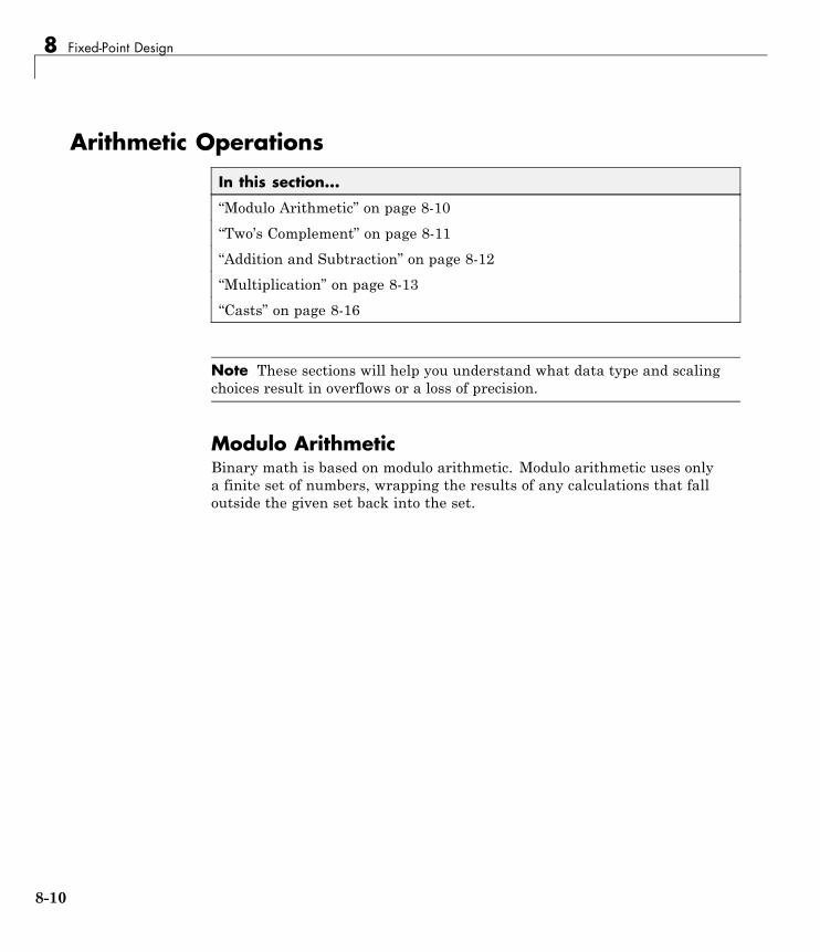
8 Fixed-Point Design
Arithmetic Operations
In this section...
“Modulo Arithmetic” on page 8-10
“Two’s Complement” on page 8-11
“Addition and Subtraction” on page 8-12
“Multiplication” on page 8-13
“Casts” on page 8-16
Note These sections will help you understand what data type and scalingchoices result in overflows or a loss of precision.
Modulo ArithmeticBinary math is based on modulo arithmetic. Modulo arithmetic uses onlya finite set of numbers, wrapping the results of any calculations that falloutside the given set back into the set.
8-10
Arithmetic Operations
For example, the common everyday clock uses modulo 12 arithmetic. Numbersin this system can only be 1 through 12. Therefore, in the “clock” system, 9plus 9 equals 6. This can be more easily visualized as a number circle:
Similarly, binary math can only use the numbers 0 and 1, and any arithmeticresults that fall outside this range are wrapped “around the circle” to either 0or 1.
Two’s ComplementTwo’s complement is a way to interpret a binary number. In two’scomplement, positive numbers always start with a 0 and negative numbersalways start with a 1. If the leading bit of a two’s complement number is 0,the value is obtained by calculating the standard binary value of the number.If the leading bit of a two’s complement number is 1, the value is obtained byassuming that the leftmost bit is negative, and then calculating the binaryvalue of the number. For example,
8-11

8 Fixed-Point Design
01 0 2 1
11 2 2 2 1 1
0
1 0
( )
(( ) ( )) ( )
To compute the negative of a binary number using two’s complement,
1 Take the one’s complement, or “flip the bits.”
2 Add a 1 using binary math.
3 Discard any bits carried beyond the original word length.
For example, consider taking the negative of 11010 (-6). First, take the one’scomplement of the number, or flip the bits:
11010 00101
Next, add a 1, wrapping all numbers to 0 or 1:
001011
00110 6
( )
Addition and SubtractionThe addition of fixed-point numbers requires that the binary points of theaddends be aligned. The addition is then performed using binary arithmeticso that no number other than 0 or 1 is used.
For example, consider the addition of 010010.1 (18.5) with 0110.110 (6.75):
010010 10110 110
011001 010
18 56 75
25 25
.
.
.
( . )( . )
( . )
Fixed-point subtraction is equivalent to adding while using the two’scomplement value for any negative values. In subtraction, the addends
8-12

Arithmetic Operations
must be sign extended to match each other’s length. For example, considersubtracting 0110.110 (6.75) from 010010.1 (18.5):
Most fixed-point DSP System Toolbox blocks that perform addition cast theadder inputs to an accumulator data type before performing the addition.Therefore, no further shifting is necessary during the addition to line up thebinary points. See “Casts” on page 8-16 for more information.
MultiplicationThe multiplication of two’s complement fixed-point numbers is directlyanalogous to regular decimal multiplication, with the exception that theintermediate results must be sign extended so that their left sides alignbefore you add them together.
For example, consider the multiplication of 10.11 (-1.25) with 011 (3):
Multiplication Data TypesThe following diagrams show the data types used for fixed-point multiplicationin the System Toolbox software. The diagrams illustrate the differencesbetween the data types used for real-real, complex-real, and complex-complex
8-13

8 Fixed-Point Design
multiplication. See individual reference pages to determine whether aparticular block accepts complex fixed-point inputs.
In most cases, you can set the data types used during multiplication in theblock mask. See Accumulator Parameters, Intermediate Product Parameters,Product Output Parameters, and Output Parameters. These data types aredefined in “Casts” on page 8-16.
Note The following diagrams show the use of fixed-point data types inmultiplication in System Toolbox software. They do not represent actualsubsystems used by the software to perform multiplication.
Real-Real Multiplication. The following diagram shows the data typesused in the multiplication of two real numbers in System Toolbox software.The software returns the output of this operation in the product output datatype, as the next figure shows.
Real-Complex Multiplication. The following diagram shows the data typesused in the multiplication of a real and a complex fixed-point number inSystem Toolbox software. Real-complex and complex-real multiplication areequivalent. The software returns the output of this operation in the productoutput data type, as the next figure shows.
8-14

Arithmetic Operations
Complex-Complex Multiplication. The following diagram shows themultiplication of two complex fixed-point numbers in System Toolboxsoftware. Note that the software returns the output of this operation in theaccumulator output data type, as the next figure shows.
8-15
8 Fixed-Point Design
System Toolbox blocks cast to the accumulator data type before performingaddition or subtraction operations. In the preceding diagram, this isequivalent to the C code
acc=ac;acc-=bd;
for the subtractor, and
acc=ad;acc+=bc;
for the adder, where acc is the accumulator.
CastsMany fixed-point System Toolbox blocks that perform arithmetic operationsallow you to specify the accumulator, intermediate product, and productoutput data types, as applicable, as well as the output data type of the block.This section gives an overview of the casts to these data types, so that you cantell if the data types you select will invoke sign extension, padding with zeros,rounding, and/or overflow.
Casts to the Accumulator Data TypeFor most fixed-point System Toolbox blocks that perform addition orsubtraction, the operands are first cast to an accumulator data type. Mostof the time, you can specify the accumulator data type on the block mask.See Accumulator Parameters. Since the addends are both cast to the sameaccumulator data type before they are added together, no extra shift isnecessary to insure that their binary points align. The result of the additionremains in the accumulator data type, with the possibility of overflow.
Casts to the Intermediate Product or Product Output Data TypeFor System Toolbox blocks that perform multiplication, the output of themultiplier is placed into a product output data type. Blocks that then feed theproduct output back into the multiplier might first cast it to an intermediateproduct data type. Most of the time, you can specify these data types on theblock mask. See Intermediate Product Parameters and Product OutputParameters.
8-16
Arithmetic Operations
Casts to the Output Data TypeMany fixed-point System Toolbox blocks allow you to specify the data type andscaling of the block output on the mask. Remember that the software doesnot allow mixed types on the input and output ports of its blocks. Therefore,if you would like to specify a fixed-point output data type and scaling for aSystem Toolbox block that supports fixed-point data types, you must feed theinput port of that block with a fixed-point signal. The final cast made by afixed-point System Toolbox block is to the output data type of the block.
Note that although you can not mix fixed-point and floating-point signalson the input and output ports of blocks, you can have fixed-point signalswith different word and fraction lengths on the ports of blocks that supportfixed-point signals.
Casting ExamplesIt is important to keep in mind the ramifications of each cast when selectingthese intermediate data types, as well as any other intermediate fixed-pointdata types that are allowed by a particular block. Depending upon the datatypes you select, overflow and/or rounding might occur. The following twoexamples demonstrate cases where overflow and rounding can occur.
8-17
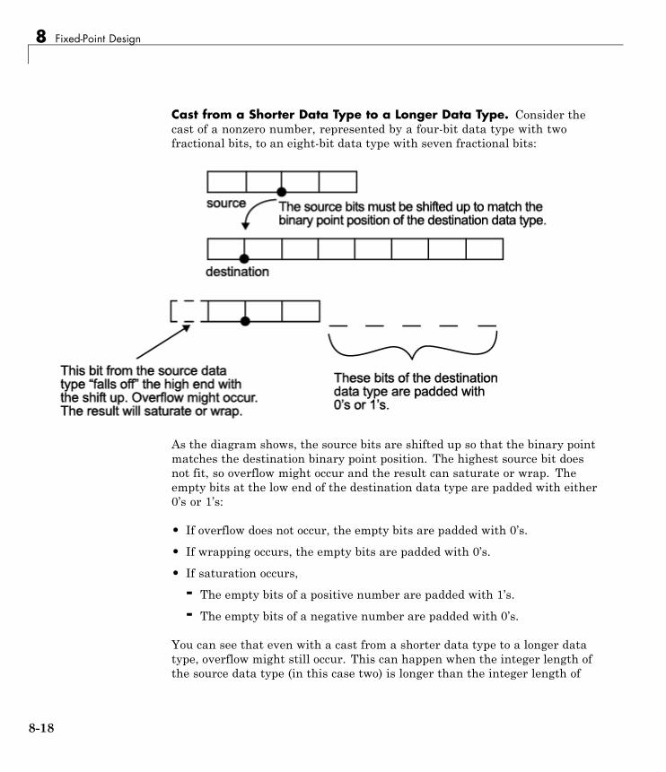
8 Fixed-Point Design
Cast from a Shorter Data Type to a Longer Data Type. Consider thecast of a nonzero number, represented by a four-bit data type with twofractional bits, to an eight-bit data type with seven fractional bits:
As the diagram shows, the source bits are shifted up so that the binary pointmatches the destination binary point position. The highest source bit doesnot fit, so overflow might occur and the result can saturate or wrap. Theempty bits at the low end of the destination data type are padded with either0’s or 1’s:
• If overflow does not occur, the empty bits are padded with 0’s.
• If wrapping occurs, the empty bits are padded with 0’s.
• If saturation occurs,
- The empty bits of a positive number are padded with 1’s.
- The empty bits of a negative number are padded with 0’s.
You can see that even with a cast from a shorter data type to a longer datatype, overflow might still occur. This can happen when the integer length ofthe source data type (in this case two) is longer than the integer length of
8-18
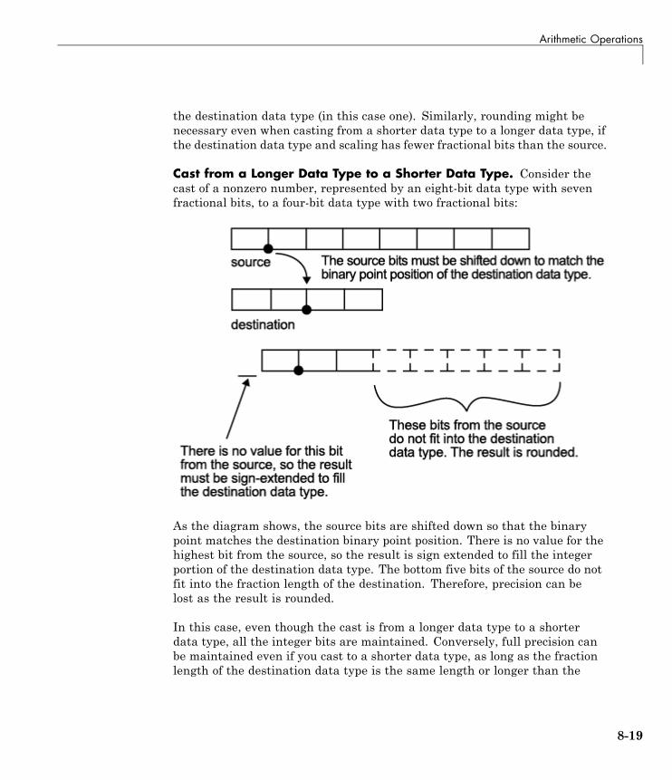
Arithmetic Operations
the destination data type (in this case one). Similarly, rounding might benecessary even when casting from a shorter data type to a longer data type, ifthe destination data type and scaling has fewer fractional bits than the source.
Cast from a Longer Data Type to a Shorter Data Type. Consider thecast of a nonzero number, represented by an eight-bit data type with sevenfractional bits, to a four-bit data type with two fractional bits:
As the diagram shows, the source bits are shifted down so that the binarypoint matches the destination binary point position. There is no value for thehighest bit from the source, so the result is sign extended to fill the integerportion of the destination data type. The bottom five bits of the source do notfit into the fraction length of the destination. Therefore, precision can belost as the result is rounded.
In this case, even though the cast is from a longer data type to a shorterdata type, all the integer bits are maintained. Conversely, full precision canbe maintained even if you cast to a shorter data type, as long as the fractionlength of the destination data type is the same length or longer than the
8-19

8 Fixed-Point Design
fraction length of the source data type. In that case, however, bits are lostfrom the high end of the result and overflow might occur.
The worst case occurs when both the integer length and the fraction length ofthe destination data type are shorter than those of the source data type andscaling. In that case, both overflow and a loss of precision can occur.
8-20

Fixed-Point Support for MATLAB® System Objects
Fixed-Point Support for MATLAB System Objects
In this section...
“Get Information About Fixed-Point System Objects” on page 8-21
“Display Fixed-Point Properties for System Objects” on page 8-25
“Set System Object Fixed-Point Properties” on page 8-26
“Full Precision for Fixed-Point System Objects” on page 8-27
Get Information About Fixed-Point System ObjectsSystem objects that support fixed-point data processing have fixed-pointproperties, which you can display for a particular object by typingdsp.<ObjectName>.helpFixedPoint at the command line. See “DisplayFixed-Point Properties for System Objects” on page 8-25 to set the display ofSystem object fixed-point properties.
The following signal processing System objects support fixed-point dataprocessing.
DSP System Toolbox System Objects that Support Fixed Point
Object Description
Estimation
dsp.LevinsonSolver Solve linear system of equations usingLevinson-Durbin recursion
Filters
dsp.AllpoleFilter IIR Filter with no zeros
dsp.BiquadFilter Model biquadratic IIR (SOS) filters
dsp.CICDecimator Decimate inputs using a CascadedIntegrator-Comb (CIC) filter
dsp.CICInterpolator Interpolate inputs using a CascadedIntegrator-Comb (CIC) filter
8-21
8 Fixed-Point Design
(Continued)
Object Description
dsp.DigitalFilter Filter each channel of input over time usingdiscrete-time filter implementations
dsp.FIRDecimator Filter and downsample input signals
dsp.FIRFilter Static or time-varying FIR filter
dsp.FIRInterpolator Upsample and filter input signals
dsp.FIRRateConverter Upsample, filter and downsample inputsignals
dsp.IIRFilter Infinite Impulse Response (IIR) filter
dsp.LMSFilter Compute output, error, and weights usingLMS adaptive algorithm
dsp.SubbandAnalysisFilter Decompose signal into high-frequency andlow-frequency subbands
dsp.SubbandSynthesisFilter Reconstruct a signal from high-frequencyand low-frequency subbands
Math Functions
dsp.ArrayVectorAdder Add vector to array along specifieddimension
dsp.ArrayVectorDivider Divide array by vector along specifieddimension
dsp.ArrayVectorMultiplier Multiply array by vector along specifieddimension
dsp.ArrayVectorSubtractor Subtract vector from array along specifieddimension
dsp.CumulativeProduct Compute cumulative product of channel,column, or row elements
dsp.CumulativeSum Compute cumulative sum of channel,column, or row elements
8-22
Fixed-Point Support for MATLAB® System Objects
(Continued)
Object Description
dsp.LDLFactor Factor square Hermitian positive definitematrices into lower, upper, and diagonalcomponents
dsp.LevinsonSolver Solve linear system of equations usingLevinson-Durbin recursion
dsp.LowerTriangularSolver Solve LX = B for X when L is lowertriangular matrix
dsp.LUFactor Factor square matrix into lower and uppertriangular matrices
dsp.Normalizer Normalize input
dsp.UpperTriangularSolver Solve UX = B for X when U is uppertriangular matrix
Quantizers
dsp.ScalarQuantizerDecoder Convert each index value into quantizedoutput value
dsp.ScalarQuantizerEncoder Perform scalar quantization encoding
dsp.VectorQuantizerDecoder Find vector quantizer codeword for givenindex value
dsp.VectorQuantizerEncoder Perform vector quantization encoding
Signal Management
dsp.Buffer Buffer an input signal
dsp.Counter Count up or down through specified rangeof numbers
Signal Operations
dsp.Convolver Compute convolution of two inputs
dsp.DigitalDownConverter Digitally down convert the input signal
dsp.DigitalUpConverter Digitally up convert the input signal
8-23
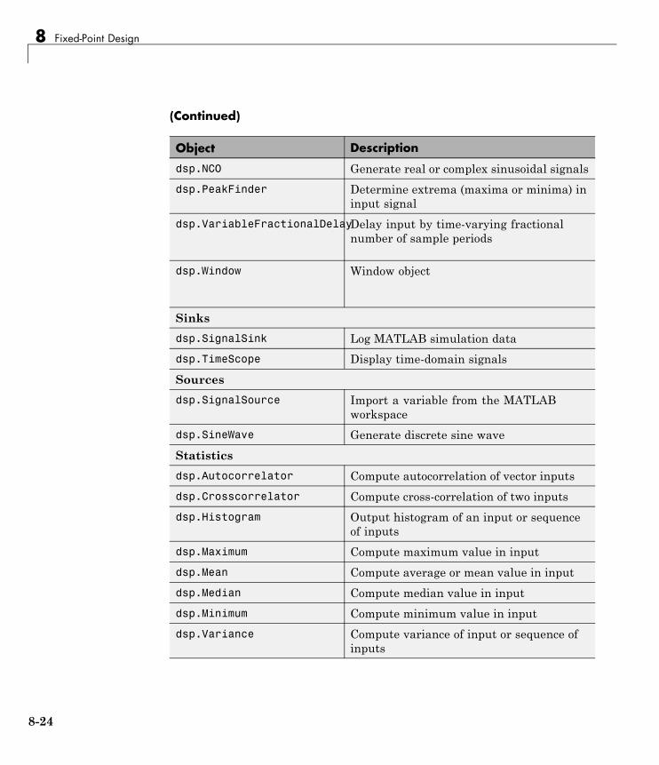
8 Fixed-Point Design
(Continued)
Object Description
dsp.NCO Generate real or complex sinusoidal signals
dsp.PeakFinder Determine extrema (maxima or minima) ininput signal
dsp.VariableFractionalDelayDelay input by time-varying fractionalnumber of sample periods
dsp.Window Window object
Sinks
dsp.SignalSink Log MATLAB simulation data
dsp.TimeScope Display time-domain signals
Sources
dsp.SignalSource Import a variable from the MATLABworkspace
dsp.SineWave Generate discrete sine wave
Statistics
dsp.Autocorrelator Compute autocorrelation of vector inputs
dsp.Crosscorrelator Compute cross-correlation of two inputs
dsp.Histogram Output histogram of an input or sequenceof inputs
dsp.Maximum Compute maximum value in input
dsp.Mean Compute average or mean value in input
dsp.Median Compute median value in input
dsp.Minimum Compute minimum value in input
dsp.Variance Compute variance of input or sequence ofinputs
8-24

Fixed-Point Support for MATLAB® System Objects
(Continued)
Object Description
Transforms
dsp.DCT Compute discrete cosine transform (DCT)of input
dsp.FFT Compute fast Fourier transform (FFT) ofinput
dsp.IDCT Compute inverse discrete cosine transform(IDCT) of input
dsp.IFFT Compute inverse fast Fourier transform(IFFT) of input
Display Fixed-Point Properties for System ObjectsYou can control whether the software displays fixed-point properties witheither of the following commands:
• matlab.system.showFixedPointProperties
• matlab.system.hideFixedPointProperties
at the MATLAB command line. These commands set the Show fixed-pointproperties display option. You can also set the display option directly viathe MATLAB preferences dialog box. Click Preferences on the MATLABToolstrip. The Preferences dialog box opens. Scroll down and sselect SystemObjects. Finally, select or deselect Show fixed-point properties.
8-25

8 Fixed-Point Design
If an object supports fixed-point data processing, its fixed-point properties areactive regardless of whether they are displayed or not.
Set System Object Fixed-Point PropertiesA number of properties affect the fixed-point data processing used by aSystem object. Objects perform fixed-point processing and use the currentfixed-point property settings when they receive fixed-point input.
You change the values of fixed-point properties in the same way as youchange any System object property value. See “Configure Components forYour System”. You also use the Fixed-Point Designer numerictype object to
8-26
Fixed-Point Support for MATLAB® System Objects
specify the desired data type as fixed-point, the signedness, and the word-and fraction-lengths. System objects support these values of DataTypeMode:Boolean, Double, Single, and Fixed-point: binary point scaling.
In the same way as for blocks, the data type properties of many Systemobjects can set the appropriate word lengths and scalings automatically byusing full precision. System objects assume that the target specified on theConfiguration Parameters Hardware Implementation target is ASIC/FPGA.
If you have not set the property that activates a dependent property and youattempt to change that dependent property, a warning message displays. Forexample, for the dsp.FFT object, before you set CustomOutputDataType tonumerictype(1,32,30) you must set OutputDataType to 'Custom'.
Note System objects do not support fixed-point word lengths greater than128 bits.
For any System object provided in the Toolbox, the fimath settings for anyfimath attached to a fi input or a fi property are ignored. Outputs from aSystem object never have an attached fimath.
Full Precision for Fixed-Point System ObjectsFullPrecisionOverride is a convenience property that, when you set totrue, automatically sets the appropriate properties for an object to usefull-precision to process fixed-point input. For System objects, full precision,fixed-point operation refers to growing just enough additional bits to computethe ideal full precision result. This operation has no minimum or maximumrange overflow nor any precision loss due to rounding or underflow. It isalso independent of any hardware-specific settings. The data types chosenare based only on known data type ranges and not on actual numeric values.Unlike full precision for dfilt objects, full precision for System objects doesnot optimize coefficient values.
When you set the FullPrecisionOverride property to true, the otherfixed-point properties it controls no longer apply and any of their non-defaultvalues are ignored. These properties are also hidden. To specify individualfixed-point properties, you must first set FullPrecisionOverride to false.
8-27

8 Fixed-Point Design
Specify Fixed-Point Attributes for Blocks
In this section...
“Fixed-Point Block Parameters” on page 8-28
“Specify System-Level Settings” on page 8-31
“Inherit via Internal Rule” on page 8-32
“Specify Data Types for Fixed-Point Blocks” on page 8-43
Fixed-Point Block ParametersSystem Toolbox blocks that have fixed-point support usually allow you tospecify fixed-point characteristics through block parameters. By specifyingdata type and scaling information for these fixed-point parameters, you cansimulate your target hardware more closely.
Note Floating-point inheritance takes precedence over the settings discussedin this section. When the block has floating-point input, all block data typesmatch the input.
You can find most fixed-point parameters on the Data Types pane of SystemToolbox blocks. The following figure shows a typical Data Types pane.
8-28
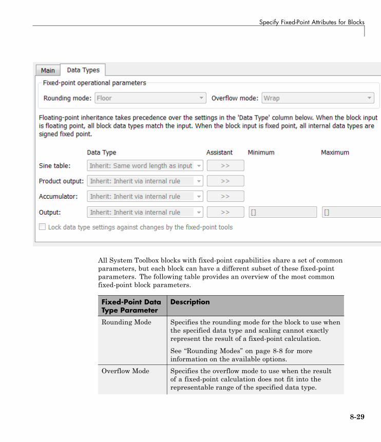
Specify Fixed-Point Attributes for Blocks
All System Toolbox blocks with fixed-point capabilities share a set of commonparameters, but each block can have a different subset of these fixed-pointparameters. The following table provides an overview of the most commonfixed-point block parameters.
Fixed-Point DataType Parameter
Description
Rounding Mode Specifies the rounding mode for the block to use whenthe specified data type and scaling cannot exactlyrepresent the result of a fixed-point calculation.
See “Rounding Modes” on page 8-8 for moreinformation on the available options.
Overflow Mode Specifies the overflow mode to use when the resultof a fixed-point calculation does not fit into therepresentable range of the specified data type.
8-29

8 Fixed-Point Design
Fixed-Point DataType Parameter
Description
See “Overflow Handling” on page 8-7 for moreinformation on the available options.
IntermediateProduct
Specifies the data type and scaling of the intermediateproduct for fixed-point blocks. Blocks that feedmultiplication results back to the input of themultiplier use the intermediate product data type.
See the reference page of a specific block to learnabout the intermediate product data type for thatblock.
Product Output Specifies the data type and scaling of the productoutput for fixed-point blocks that must computemultiplication results.
See the reference page of a specific block to learnabout the product output data type for that block. Foror complex-complex multiplication, the multiplicationresult is in the accumulator data type. See“Multiplication Data Types” on page 8-13 for moreinformation on complex fixed-point multiplication inSystem toolbox software.
Accumulator Specifies the data type and scaling of the accumulator(sum) for fixed-point blocks that must hold summationresults for further calculation. Most such blocks castto the accumulator data type before performing theadd operations (summation).
See the reference page of a specific block for details onthe accumulator data type of that block.
Output Specifies the output data type and scaling for blocks.
8-30
Specify Fixed-Point Attributes for Blocks
Using the Data Type AssistantThe Data Type Assistant is an interactive graphical tool available on theData Types pane of some fixed-point System Toolbox blocks.
To learn more about using the Data Type Assistant to help you specifyblock data type parameters, see the following section of the Simulinkdocumentation:
“Specify Data Types Using Data Type Assistant”
Checking Signal RangesSome fixed-point System Toolbox blocks have Minimum and Maximumparameters on the Data Types pane. When a fixed-point data type has theseparameters, you can use them to specify appropriate minimum and maximumvalues for range checking purposes.
To learn how to specify signal ranges and enable signal range checking, see“Signal Ranges” in the Simulink documentation.
Specify System-Level SettingsYou can monitor and control fixed-point settings for System Toolbox blocksat a system or subsystem level with the Fixed-Point Tool. For additionalinformation on these subjects, see
• The fxptdlg reference page — A reference page on the Fixed-Point Tool inthe Simulink documentation
• “Fixed-Point Tool” — A tutorial that highlights the use of the Fixed-PointTool in the Fixed-Point Designer software documentation
LoggingThe Fixed-Point Tool logs overflows, saturations, and simulation minimumsand maximums for fixed-point System Toolbox blocks. The Fixed-Point Tooldoes not log overflows and saturations when the Data overflow line in theDiagnostics > Data Integrity pane of the Configuration Parameters dialogbox is set to None.
8-31

8 Fixed-Point Design
AutoscalingYou can use the Fixed-Point Tool autoscaling feature to set the scaling forSystem Toolbox fixed-point data types.
Data type overrideSystem Toolbox blocks obey the Use local settings, Double, Single, andOff modes of the Data type override parameter in the Fixed-Point Tool.The Scaled double mode is also supported for System Toolboxes source andbyte-shuffling blocks, and for some arithmetic blocks such as Difference andNormalization.
Inherit via Internal RuleSelecting appropriate word lengths and scalings for the fixed-point parametersin your model can be challenging. To aid you, an Inherit via internalrule choice is often available for fixed-point block data type parameters,such as the Accumulator and Product output signals. The followingsections describe how the word and fraction lengths are selected for you whenyou choose Inherit via internal rule for a fixed-point block data typeparameter in System Toolbox software:
• “Internal Rule for Accumulator Data Types” on page 8-32
• “Internal Rule for Product Data Types” on page 8-33
• “Internal Rule for Output Data Types” on page 8-34
• “The Effect of the Hardware Implementation Pane on the Internal Rule”on page 8-34
• “Internal Rule Examples” on page 8-36
Note In the equations in the following sections, WL = word length and FL =fraction length.
Internal Rule for Accumulator Data TypesThe internal rule for accumulator data types first calculates the ideal,full-precision result. Where N is the number of addends:
8-32

Specify Fixed-Point Attributes for Blocks
WL WL Nideal accumulator input to accumulator floor(log ( )2 1 )) 1
FL FLideal accumulator input to accumulator
For example, consider summing all the elements of a vector of length 6 anddata type sfix10_En8. The ideal, full-precision result has a word length of13 and a fraction length of 8.
The accumulator can be real or complex. The preceding equations are used forboth the real and imaginary parts of the accumulator. For any calculation,after the full-precision result is calculated, the final word and fraction lengthsset by the internal rule are affected by your particular hardware. See “TheEffect of the Hardware Implementation Pane on the Internal Rule” on page8-34 for more information.
Internal Rule for Product Data TypesThe internal rule for product data types first calculates the ideal, full-precisionresult:
WL WL WLideal product input 1 input 2
FL FL FLideal product input 1 input 2
For example, multiplying together the elements of a real vector of length 2and data type sfix10_En8. The ideal, full-precision result has a word length of20 and a fraction length of 16.
For real-complex multiplication, the ideal word length and fraction length isused for both the complex and real portion of the result. For complex-complexmultiplication, the ideal word length and fraction length is used for the partialproducts, and the internal rule for accumulator data types described aboveis used for the final sums. For any calculation, after the full-precision resultis calculated, the final word and fraction lengths set by the internal ruleare affected by your particular hardware. See “The Effect of the HardwareImplementation Pane on the Internal Rule” on page 8-34 for more information.
8-33
8 Fixed-Point Design
Internal Rule for Output Data TypesA few System Toolbox blocks have an Inherit via internal rule choiceavailable for the block output. The internal rule used in these cases isblock-specific, and the equations are listed in the block reference page.
As with accumulator and product data types, the final output word andfraction lengths set by the internal rule are affected by your particularhardware, as described in “The Effect of the Hardware Implementation Paneon the Internal Rule” on page 8-34.
The Effect of the Hardware Implementation Pane on theInternal RuleThe internal rule selects word lengths and fraction lengths that areappropriate for your hardware. To get the best results using the internalrule, you must specify the type of hardware you are using on the HardwareImplementation pane of the Configuration Parameters dialog box. You canopen this dialog box from the Simulation menu in your model.
8-34

Specify Fixed-Point Attributes for Blocks
ASIC/FPGA. On an ASIC/FPGA target, the ideal, full-precision word lengthand fraction length calculated by the internal rule are used. If the calculatedideal word length is larger than the largest allowed word length, you receivean error. The largest word length allowed for Simulink and System Toolboxsoftware is 128 bits.
Other targets. For all targets other than ASIC/FPGA, the ideal,full-precision word length calculated by the internal rule is rounded up to thenext available word length of the target. The calculated ideal fraction lengthis used, keeping the least-significant bits.
If the calculated ideal word length for a product data type is larger than thelargest word length on the target, you receive an error. If the calculated idealword length for an accumulator or output data type is larger than the largestword length on the target, the largest target word length is used.
8-35

8 Fixed-Point Design
Internal Rule ExamplesThe following sections show examples of how the internal rule interacts withthe Hardware Implementation pane to calculate accumulator data typesand product data types.
Accumulator Data Types. Consider the following modelex_internalRule_accumExp.
In the Difference blocks, the Accumulator parameter is set to Inherit:Inherit via internal rule, and the Output parameter is set to Inherit:Same as accumulator. Therefore, you can see the accumulator data typecalculated by the internal rule on the output signal in the model.
In the preceding model, the Device type parameter in the HardwareImplementation pane of the Configuration Parameters dialog box is set to
8-36

Specify Fixed-Point Attributes for Blocks
ASIC/FPGA. Therefore, the accumulator data type used by the internal rule isthe ideal, full-precision result.
Calculate the full-precision word length for each of the Difference blocks inthe model:
WL WL numbideal accumulator input to accumulator floor(log (2 eer of accumulations
WLideal accumulator
))
floor(log (2
1
9 1)))
1
9 0 1 10
1
WL
WL WL
ideal accumulator
ideal accumulator inpput to accumulator number of accumulations1 floor(log ( ))2 11
16 1 11WL
WLideal accumulator
ideal accumula
floor(log ( ))2
ttor
ideal accumulator input to accumulatorWL WL
1
2
16 0 1 17
22 1 floor(log ( ))2 number of accumulations
WLideal accumulatoor
ideal accumulatorWL2
2
127 1 1
127 0 1 128
floor(log ( ))2
Calculate the full-precision fraction length, which is the same for each MatrixSum block in this example:
FL FL
FLideal accumulator input to accumulator
ideal accumula
ttor 4
Now change the Device type parameter in the Hardware Implementationpane of the Configuration Parameters dialog box to 32 bit EmbeddedProcessor, by changing the parameters as shown in the following figure.
8-37
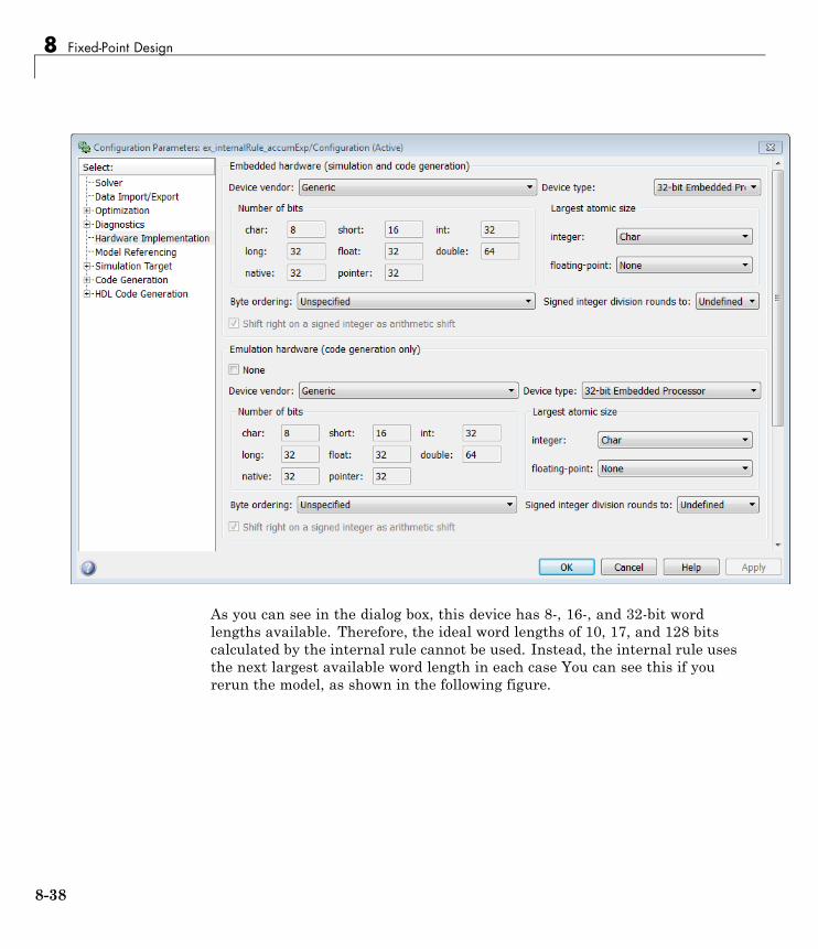
8 Fixed-Point Design
As you can see in the dialog box, this device has 8-, 16-, and 32-bit wordlengths available. Therefore, the ideal word lengths of 10, 17, and 128 bitscalculated by the internal rule cannot be used. Instead, the internal rule usesthe next largest available word length in each case You can see this if yourerun the model, as shown in the following figure.
8-38

Specify Fixed-Point Attributes for Blocks
8-39
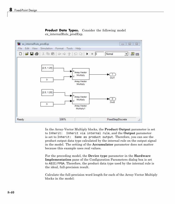
8 Fixed-Point Design
Product Data Types. Consider the following modelex_internalRule_prodExp.
In the Array-Vector Multiply blocks, the Product Output parameter is setto Inherit: Inherit via internal rule, and the Output parameteris set to Inherit: Same as product output. Therefore, you can see theproduct output data type calculated by the internal rule on the output signalin the model. The setting of the Accumulator parameter does not matterbecause this example uses real values.
For the preceding model, the Device type parameter in the HardwareImplementation pane of the Configuration Parameters dialog box is setto ASIC/FPGA. Therefore, the product data type used by the internal rule isthe ideal, full-precision result.
Calculate the full-precision word length for each of the Array-Vector Multiplyblocks in the model:
8-40

Specify Fixed-Point Attributes for Blocks
WL WL WL
WL
W
ideal product input a input b
ideal product
7 5 12
LL WL WL
WLideal product input a input b
ideal product
1
1 16 15
31
Calculate the full-precision fraction length, which is the same for eachArray-Vector Multiply block in this example:
FL FL
FLideal accumulator input to accumulator
ideal accumula
ttor 4
Now change the Device type parameter in the Hardware Implementationpane of the Configuration Parameters dialog box to 32 bit EmbeddedProcessor, as shown in the following figure.
8-41
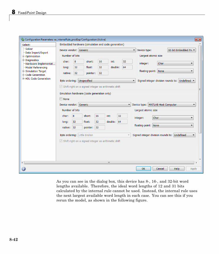
8 Fixed-Point Design
As you can see in the dialog box, this device has 8-, 16-, and 32-bit wordlengths available. Therefore, the ideal word lengths of 12 and 31 bitscalculated by the internal rule cannot be used. Instead, the internal rule usesthe next largest available word length in each case. You can see this if yourerun the model, as shown in the following figure.
8-42
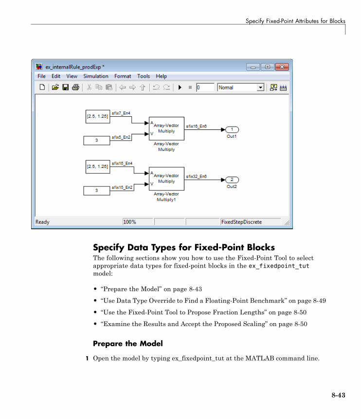
Specify Fixed-Point Attributes for Blocks
Specify Data Types for Fixed-Point BlocksThe following sections show you how to use the Fixed-Point Tool to selectappropriate data types for fixed-point blocks in the ex_fixedpoint_tutmodel:
• “Prepare the Model” on page 8-43
• “Use Data Type Override to Find a Floating-Point Benchmark” on page 8-49
• “Use the Fixed-Point Tool to Propose Fraction Lengths” on page 8-50
• “Examine the Results and Accept the Proposed Scaling” on page 8-50
Prepare the Model
1 Open the model by typing ex_fixedpoint_tut at the MATLAB command line.
8-43

8 Fixed-Point Design
This model uses the Cumulative Sum block to sum the input coming from theFixed-Point Sources subsystem. The Fixed-Point Sources subsystem outputstwo signals with different data types:
• The Signed source has a word length of 16 bits and a fraction length of15 bits.
• The Unsigned source has a word length of 16 bits and a fraction length of16 bits.
2 Run the model to check for overflow. MATLAB displays the followingwarnings at the command line:
Warning: Overflow occurred. This originated from'ex_fixedpoint_tut/Signed Cumulative Sum'.Warning: Overflow occurred. This originated from
8-44

Specify Fixed-Point Attributes for Blocks
'ex_fixedpoint_tut/Unsigned Cumulative Sum'.
According to these warnings, overflow occurs in both Cumulative Sum blocks.
3 To investigate the overflows in this model, use the Fixed-Point Tool. You canopen the Fixed-Point Tool by selecting Tools > Fixed-Point > Fixed-PointTool from the model menu. Turn on logging for all blocks in your model bysetting the Fixed-point instrumentation mode parameter to Minimums,maximums and overflows.
4 Now that you have turned on logging, rerun the model by clicking theSimulation button.
8-45

8 Fixed-Point Design
8-46

Specify Fixed-Point Attributes for Blocks
• Name — Provides the name of each signal in the following format:Subsystem Name/Block Name: Signal Name.
• SimDT — The simulation data type of each logged signal.
• SpecifiedDT— The data type specified on the block dialog for each signal.
• SimMin — The smallest representable value achieved during simulationfor each logged signal.
• SimMax — The largest representable value achieved during simulationfor each logged signal.
• OverflowWraps— The number of overflows that wrap during simulation.
For more information on each of the columns in this table, see the “ContentsPane” section of the Simulink fxptdlg function reference page.
You can also see that the SimMin and SimMax values for the Accumulatordata types range from 0 to .9997. The logged results indicate that 8,192overflows wrapped during simulation in the Accumulator data type of theSigned Cumulative Sum block. Similarly, the Accumulator data type ofthe Unsigned Cumulative Sum block had 16,383 overflows wrap duringsimulation.
To get more information about each of these data types, highlight them in theContents pane, and click the Show details for selected result button
( )
6 Assume a target hardware that supports 32-bit integers, and set theAccumulator word length in both Cumulative Sum blocks to 32. To do so,perform the following steps:
a Right-click the Signed Cumulative Sum: Accumulator row in theFixed-Point Tool pane, and select Highlight Block In Model.
b Double-click the block in the model, and select the Data Types paneof the dialog box.
c Open the Data Type Assistant for Accumulator by clicking the
Assistant button ( ) in the Accumulator data type row.
8-47

8 Fixed-Point Design
d Set the Mode to Fixed Point. To see the representable range of thecurrent specified data type, click the Fixed-point details link. The tooldisplays the representable maximum and representable minimum valuesfor the current data type.
e Change the Word length to 32, and click the Refresh details button inthe Fixed-point details section to see the updated representable range.
8-48

Specify Fixed-Point Attributes for Blocks
When you change the value of theWord length parameter, the data typestring in the Data Type edit box automatically updates.
f ClickOK on the block dialog box to save your changes and close the window.
g Set the word length of the Accumulator data type of the UnsignedCumulative Sum block to 32 bits. You can do so in one of two ways:
• Type the data type string fixdt([],32,0) directly into Data Type editbox for the Accumulator data type parameter.
• Perform the same steps you used to set the word length of theAccumulator data type of the Signed Cumulative Sum block to 32 bits.
7 To verify your changes in word length and check for overflow, rerun yourmodel. To do so, click the Simulate button in the Fixed-Point Tool.
The Contents pane of the Fixed-Point Tool updates, and you can see that nooverflows occurred in the most recent simulation. However, you can also seethat the SimMin and SimMax values range from 0 to 0. This underflowhappens because the fraction length of the Accumulator data type is toosmall. The SpecifiedDT cannot represent the precision of the data values.The following sections discuss how to find a floating-point benchmark and usethe Fixed-Point Tool to propose fraction lengths.
Use Data Type Override to Find a Floating-Point BenchmarkThe Data type override feature of the Fixed-Point tool allows you tooverride the data types specified in your model with floating-point types.Running your model in Double override mode gives you a reference range tohelp you select appropriate fraction lengths for your fixed-point data types.To do so, perform the following steps:
1 Open the Fixed-Point Tool and set Data type override to Double.
2 Run your model by clicking the Run simulation and store active resultsbutton.
3 Examine the results in the Contents pane of the Fixed-Point Tool. Becauseyou ran the model in Double override mode, you get an accurate, idealizedrepresentation of the simulation minimums and maximums. These valuesappear in the SimMin and SimMax parameters.
8-49

8 Fixed-Point Design
4 Now that you have an accurate reference representation of the simulationminimum and maximum values, you can more easily choose appropriatefraction lengths. Before making these choices, save your active results toreference so you can use them as your floating-point benchmark. To do so,select Results > Move Active Results To Reference from the Fixed-PointTool menu. The status displayed in the Run column changes from Active toReference for all signals in your model.
Use the Fixed-Point Tool to Propose Fraction LengthsNow that you have your Double override results saved as a floating-pointreference, you are ready to propose fraction lengths.
1 To propose fraction lengths for your data types, you must have a set of Activeresults available in the Fixed-Point Tool. To produce an active set of results,simply rerun your model. The tool now displays both the Active results andthe Reference results for each signal.
2 Select the Use simulation min/max if design min/max is not availablecheck box. You did not specify any design minimums or maximums for thedata types in this model. Thus, the tool uses the logged information to computeand propose fraction lengths. For information on specifying design minimumsand maximums, see “Signal Ranges” in the Simulink documentation.
3 Click the Propose fraction lengths button ( ). The tool populates theproposed data types in the ProposedDT column of the Contents pane. Thecorresponding proposed minimums and maximums are displayed in theProposedMin and ProposedMax columns.
Examine the Results and Accept the Proposed ScalingBefore accepting the fraction lengths proposed by the Fixed-Point Tool, it isimportant to look at the details of that data type. Doing so allows you to seehow much of your data the suggested data type can represent. To examine thesuggested data types and accept the proposed scaling, perform the followingsteps:
1 In the Contents pane of the Fixed-Point Tool, you can see the proposedfraction lengths for the data types in your model.
8-50

Specify Fixed-Point Attributes for Blocks
• The proposed fraction length for the Accumulator data type of both theSigned and Unsigned Cumulative Sum blocks is 17 bits.
• To get more details about the proposed scaling for a particular data type,highlight the data type in the Contents pane of the Fixed-Point Tool.
• Open the Autoscale Information window for the highlighted data typeby clicking the Show autoscale information for the selected result
button ( ).
2 When the Autoscale Information window opens, check the Value andPercent Proposed Representable columns for the Simulation Minimumand Simulation Maximum parameters. You can see that the proposed datatype can represent 100% of the range of simulation data.
3 To accept the proposed data types, select the check box in the Accept columnfor each data type whose proposed scaling you want to keep. Then, click the
Apply accepted fraction lengths button ( ). The tool updates thespecified data types on the block dialog boxes and the SpecifiedDT column inthe Contents pane.
4 To verify the newly accepted scaling, set the Data type override parameterback to Use local settings, and run the model. Looking at Contents pane ofthe Fixed-Point Tool, you can see the following details:
• The SimMin and SimMax values of the Active run match the SimMinand SimMax values from the floating-point Reference run.
• There are no longer any overflows.
• The SimDT does not match the SpecifiedDT for the Accumulator datatype of either Cumulative Sum block. This difference occurs because theCumulative Sum block always inherits its Signedness from the inputsignal and only allows you to specify a Signedness of Auto. Therefore,the SpecifiedDT for both Accumulator data types is fixdt([],32,17).However, because the Signed Cumulative Sum block has a signed inputsignal, the SimDT for the Accumulator parameter of that block is alsosigned (fixdt(1,32,17)). Similarly, the SimDT for the Accumulatorparameter of the Unsigned Cumulative Sum block inherits its Signednessfrom its input signal and thus is unsigned (fixdt(0,32,17)).
8-51

8 Fixed-Point Design
Quantizers
In this section...
“Scalar Quantizers” on page 8-52
“Vector Quantizers” on page 8-61
Scalar Quantizers
• “Analysis and Synthesis of Speech” on page 8-52
• “Identify Your Residual Signal and Reflection Coefficients” on page 8-54
• “Create a Scalar Quantizer” on page 8-56
Analysis and Synthesis of SpeechYou can use blocks from the DSP System Toolbox Quantizers library to designscalar quantizer encoders and decoders. A speech signal is usually representedin digital format, which is a sequence of binary bits. For storage andtransmission applications, it is desirable to compress a signal by representingit with as few bits as possible, while maintaining its perceptual quality.Quantization is the process of representing a signal with a reduced level ofprecision. If you decrease the number of bits allocated for the quantization ofyour speech signal, the signal is distorted and the speech quality degrades.
In narrowband digital speech compression, speech signals are sampled ata rate of 8000 samples per second. Each sample is typically representedby 8 bits. This corresponds to a bit rate of 64 kbits per second. Furthercompression is possible at the cost of quality. Most of the current low bit ratespeech coders are based on the principle of linear predictive speech coding.This topic shows you how to use the Scalar Quantizer Encoder and ScalarQuantizer Decoder blocks to implement a simple speech coder.
1 Type ex_sq_example1 at the MATLAB command line to open the examplemodel.
8-52
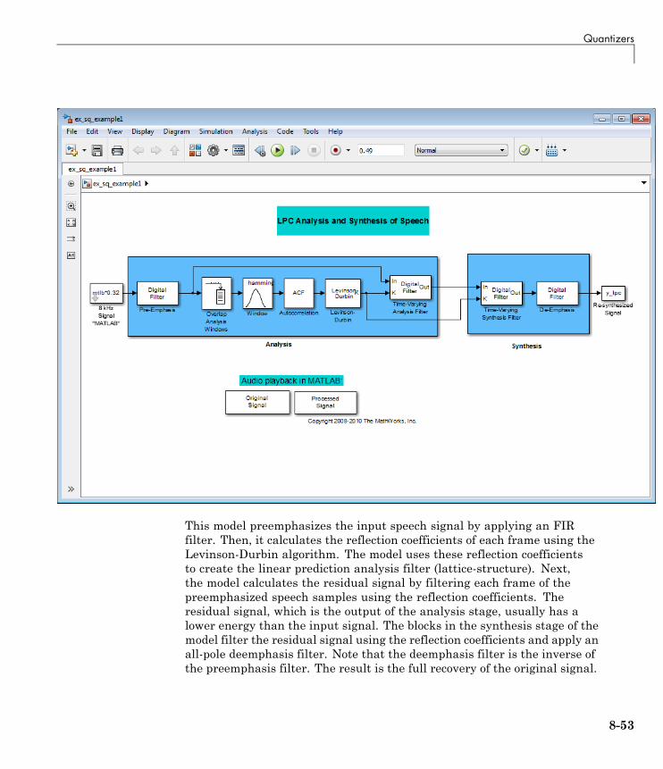
Quantizers
This model preemphasizes the input speech signal by applying an FIRfilter. Then, it calculates the reflection coefficients of each frame using theLevinson-Durbin algorithm. The model uses these reflection coefficientsto create the linear prediction analysis filter (lattice-structure). Next,the model calculates the residual signal by filtering each frame of thepreemphasized speech samples using the reflection coefficients. Theresidual signal, which is the output of the analysis stage, usually has alower energy than the input signal. The blocks in the synthesis stage of themodel filter the residual signal using the reflection coefficients and apply anall-pole deemphasis filter. Note that the deemphasis filter is the inverse ofthe preemphasis filter. The result is the full recovery of the original signal.
8-53

8 Fixed-Point Design
2 Run this model.
3 Double-click the Original Signal and Processed Signal blocks and listen toboth the original and the processed signal.
There is no significant difference between the two because no quantizationwas performed.
To better approximate a real-world speech analysis and synthesis system, youneed to quantize the residual signal and reflection coefficients before they aretransmitted. The following topics show you how to design scalar quantizers toaccomplish this task.
Identify Your Residual Signal and Reflection CoefficientsIn the previous topic, “Analysis and Synthesis of Speech” on page 8-52,you learned the theory behind the LPC Analysis and Synthesis of Speechexample model. In this topic, you define the residual signal and thereflection coefficients in your MATLAB workspace as the variables E and K,respectively. Later, you use these values to create your scalar quantizers:
1 Open the example model by typing ex_sq_example2 at the MATLABcommand line.
2 Save the model file as ex_sq_example2 in your working folder.
3 From the Sinks library, click-and-drag two Signal To Workspace blocksinto your model.
4 Connect the output of the Levinson-Durbin block to one of the Signal ToWorkspace blocks.
5 Double-click this Signal To Workspace block and set the Variable nameparameter to K. Click OK.
6 Connect the output of the Time-Varying Analysis Filter block to the otherSignal To Workspace block.
8-54
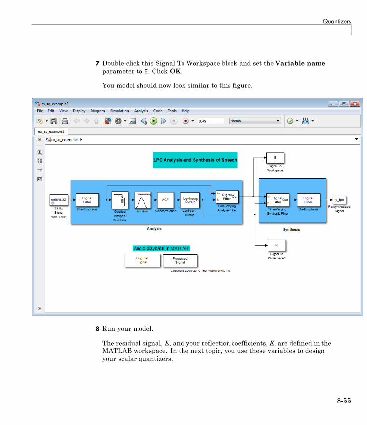
Quantizers
7 Double-click this Signal To Workspace block and set the Variable nameparameter to E. Click OK.
You model should now look similar to this figure.
8 Run your model.
The residual signal, E, and your reflection coefficients, K, are defined in theMATLAB workspace. In the next topic, you use these variables to designyour scalar quantizers.
8-55
8 Fixed-Point Design
Create a Scalar QuantizerIn this topic, you create scalar quantizer encoders and decoders to quantizethe residual signal, E, and the reflection coefficients, K:
1 If the model you created in “Identify Your Residual Signal and ReflectionCoefficients” on page 8-54 is not open on your desktop, you can open anequivalent model by typing ex_sq_example2 at the MATLAB commandprompt.
2 Run this model to define the variables E and K in the MATLAB workspace.
3 From the Quantizers library, click-and-drag a Scalar Quantizer Designblock into your model. Double-click this block to open the SQ Design ToolGUI.
4 For the Training Set parameter, enter K.
The variable K represents the reflection coefficients you want to quantize.By definition, they range from -1 to 1.
Note Theoretically, the signal that is used as the Training Set parametershould contain a representative set of values for the parameter to bequantized. However, this example provides an approximation to this globaltraining process.
5 For the Number of levels parameter, enter 128.
Assume that your compression system has 7 bits to represent eachreflection coefficient. This means it is capable of representing 27 or 128values. The Number of levels parameter is equal to the total number ofcodewords in the codebook.
6 Set the Block type parameter to Both.
7 For the Encoder block name parameter, enter SQ Encoder -Reflection Coefficients.
8 For the Decoder block name parameter, enter SQ Decoder -Reflection Coefficients.
8-56

Quantizers
9 Make sure that your desired destination model, ex_sq_example2, is thecurrent model. You can type gcs in the MATLAB Command Window todisplay the name of your current model.
8-57
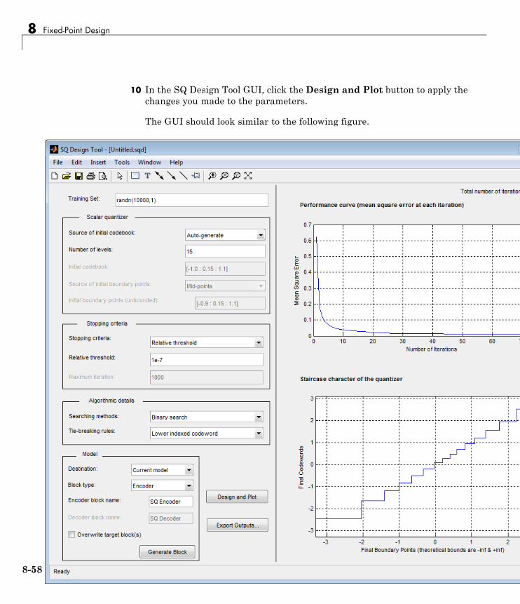
8 Fixed-Point Design
10 In the SQ Design Tool GUI, click the Design and Plot button to apply thechanges you made to the parameters.
The GUI should look similar to the following figure.
8-58

Quantizers
11 Click the Generate Model button.
Two new blocks, SQ Encoder - Reflection Coefficients and SQ Decoder -Reflection Coefficients, appear in your model file.
12 Click the SQ Design Tool GUI and, for the Training Set parameter, enterE.
13 Repeat steps 5 to 11 for the variable E, which represents the residual signalyou want to quantize. In steps 6 and 7, name your blocks SQ Encoder -Residual and SQ Decoder - Residual.
Once you have completed these steps, two new blocks, SQ Encoder -Residual and SQ Decoder - Residual, appear in your model file.
14 Close the SQ Design Tool GUI. You do not need to save the SQ DesignTool session.
You have now created a scalar quantizer encoder and a scalar quantizerdecoder for each signal you want to quantize. You are ready to quantize theresidual signal, E, and the reflection coefficients, K.
8-59

8 Fixed-Point Design
15 Save the model as ex_sq_example3. Your model should look similar tothe following figure.
16 Run your model.
17 Double-click the Original Signal and Processed Signal blocks, and listento both signals.
Again, there is no perceptible difference between the two. You can thereforeconclude that quantizing your residual and reflection coefficients did notaffect the ability of your system to accurately reproduce the input signal.
You have now quantized the residual and reflection coefficients. The bit rateof a quantization system is calculated as (bits per frame)*(frame rate).
In this example, the bit rate is [(80 residual samples/frame)*(7 bits/sample) +(12 reflection coefficient samples/frame)*(7 bits/sample)]*(100 frames/second),or 64.4 kbits per second. This is higher than most modern speech coders,
8-60
Quantizers
which typically have a bit rate of 8 to 24 kbits per second. If you decrease thenumber of bits allocated for the quantization of the reflection coefficients orthe residual signal, the overall bit rate would decrease. However, the speechquality would also degrade.
For information about decreasing the bit rate without affecting speech quality,see “Vector Quantizers” on page 8-61.
Vector Quantizers
• “Build Your Vector Quantizer Model” on page 8-61
• “Configure and Run Your Model” on page 8-63
Build Your Vector Quantizer ModelIn the previous section, you created scalar quantizer encoders and decodersand used them to quantize your residual signal and reflection coefficients.The bit rate of your scalar quantization system was 64.4 kbits per second.This bit rate is higher than most modern speech coders. To accommodate agreater number of users in each channel, you need to lower this bit rate whilemaintaining the quality of your speech signal. You can use vector quantizers,which exploit the correlations between each sample of a signal, to accomplishthis task.
In this topic, you modify your scalar quantization model so that you are usinga split vector quantizer to quantize your reflection coefficients:
1 Open a model similar to the one you created in “Create a Scalar Quantizer”on page 8-56 by typing ex_vq_example1 at the MATLAB command prompt.The example model ex_vq_example1 adds a new LSF Vector Quantizationsubsystem to the ex_sq_example3 model. This subsystem is preconfiguredto work as a vector quantizer. You can use this subsystem to encode anddecode your reflection coefficients using the split vector quantizationmethod.
2 Delete the SQ Encoder – Reflection Coefficients and SQ Decoder –Reflection Coefficients blocks.
8-61

8 Fixed-Point Design
3 From the Simulink Sinks library,click-and-drag a Terminator block intoyour model.
4 From the DSP System Toolbox Estimation > Linear Prediction library,click-and-drag a LSF/LSP to LPC Conversion block and two LPC to/fromRC blocks into your model.
5 Connect the blocks as shown in the following figure. You do not need toconnect Terminator blocks to the P ports of the LPC to/from RC blocks.These ports disappear once you set block parameters.
You have modified your model to include a subsystem capable of vectorquantization. In the next topic, you reset your model parameters to quantizeyour reflection coefficients using the split vector quantization method.
8-62

Quantizers
Configure and Run Your ModelIn the previous topic, you configured your scalar quantization model for vectorquantization by adding the LSF Vector Quantization subsystem. In this topic,you set your block parameters and quantize your reflection coefficients usingthe split vector quantization method.
1 If the model you created in “Build Your Vector Quantizer Model” on page8-61 is not open on your desktop, you can open an equivalent model bytyping ex_vq_example2 at the MATLAB command prompt.
2 Double-click the LSF Vector Quantization subsystem, and then double-clickthe LSF Split VQ subsystem.
8-63
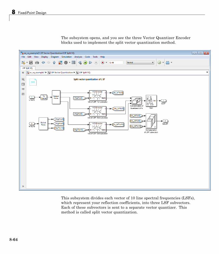
8 Fixed-Point Design
The subsystem opens, and you see the three Vector Quantizer Encoderblocks used to implement the split vector quantization method.
This subsystem divides each vector of 10 line spectral frequencies (LSFs),which represent your reflection coefficients, into three LSF subvectors.Each of these subvectors is sent to a separate vector quantizer. Thismethod is called split vector quantization.
8-64
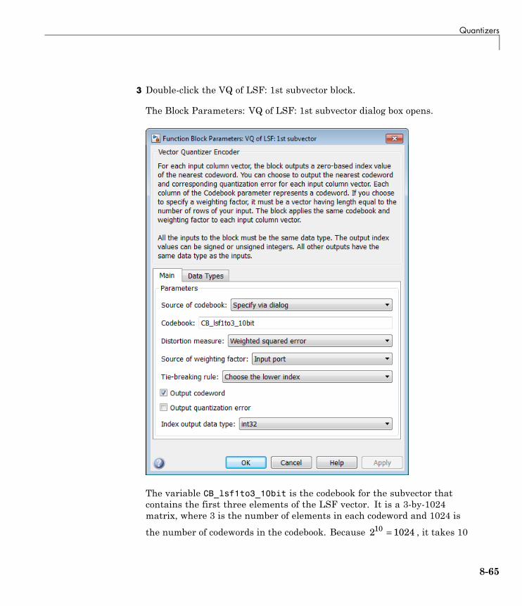
Quantizers
3 Double-click the VQ of LSF: 1st subvector block.
The Block Parameters: VQ of LSF: 1st subvector dialog box opens.
The variable CB_lsf1to3_10bit is the codebook for the subvector thatcontains the first three elements of the LSF vector. It is a 3-by-1024matrix, where 3 is the number of elements in each codeword and 1024 is
the number of codewords in the codebook. Because 2 102410 = , it takes 10
8-65
8 Fixed-Point Design
bits to quantize this first subvector. Similarly, a 10-bit vector quantizer isapplied to the second and third subvectors, which contain elements 4 to 6and 7 to 10 of the LSF vector, respectively. Therefore, it takes 30 bits toquantize all three subvectors.
Note If you used the vector quantization method to quantize yourreflection coefficients, you would need 230 or 1.0737e9 codebook valuesto achieve the same degree of accuracy as the split vector quantizationmethod.
4 In your model file, double-click the Autocorrelation block and set theMaximum non-negative lag (less than input length) parameter to10. Click OK.
This parameter controls the number of linear polynomial coefficients(LPCs) that are input to the split vector quantization method.
5 Double-click the LPC to/from RC block that is connected to the input ofthe LSF Vector Quantization subsystem. Clear the Output normalizedprediction error power check box. Click OK.
6 Double-click the LSF/LSP to LPC Conversion block and set the Inputparameter to LSF in range (0 to pi). Click OK.
7 Double-click the LPC to/from RC block that is connected to the outputof the LSF/LSP to LPC Conversion block. Set the Type of conversionparameter to LPC to RC, and clear the Output normalized predictionerror power check box. Click OK.
8 Run your model.
8-66

Quantizers
9 Double-click the Original Signal and Processed Signal blocks to listen toboth the original and the processed signal.
There is no perceptible difference between the two. Quantizing yourreflection coefficients using a split vector quantization method producedgood quality speech without much distortion.
You have now used the split vector quantization method to quantize yourreflection coefficients. The vector quantizers in the LSF Vector Quantizationsubsystem use 30 bits to quantize a frame containing 80 reflection coefficients.The bit rate of a quantization system is calculated as (bits per frame)*(framerate).
In this example, the bit rate is [(80 residual samples/frame)*(7 bits/sample) +(30 bits/frame)]*(100 frames/second), or 59 kbits per second. This is less than64.4 kbits per second, the bit rate of the scalar quantization system. However,the quality of the speech signal did not degrade. If you want to further reducethe bit rate of your system, you can use the vector quantization method toquantize the residual signal.
8-67

8 Fixed-Point Design
Fixed-Point Filter Design
In this section...
“Overview of Fixed-Point Filters” on page 8-68
“Data Types for Filter Functions” on page 8-68
“Floating-Point to Fixed-Point Filter Conversion” on page 8-70
“Create an FIR Filter Using Integer Coefficients” on page 8-80
“Fixed-Point Filtering in Simulink” on page 8-98
Overview of Fixed-Point FiltersThe most common use of fixed-point filters is in the DSP chips, where thedata storage capabilities are limited, or embedded systems and devices wherelow-power consumption is necessary. For example, the data input may comefrom a 12 bit ADC, the data bus may be 16 bit, and the multiplier may have24 bits. Within these space constraints, DSP System Toolbox software enablesyou to design the best possible fixed-point filter.
What Is a Fixed-Point Filter?lA fixed-point filter uses fixed-point arithmetic and is represented by anequation with fixed-point coefficients. To learn about fixed-point arithmetic,see “Arithmetic Operations”.
Data Types for Filter Functions
• “Data Type Support” on page 8-68
• “Fixed Data Type Support” on page 8-69
• “Single Data Type Support” on page 8-69
Data Type SupportThere are three different data types supported in DSP System Toolboxsoftware:
8-68
Fixed-Point Filter Design
• Fixed — Requires Fixed-Point Designer and is supported by packageslisted in “Fixed Data Type Support” on page 8-69.
• Double — Double precision, floating point and is the default data type forDSP System Toolbox software; accepted by all functions
• Single — Single precision, floating point and is supported by specificpackages outlined in “Single Data Type Support” on page 8-69.
Fixed Data Type SupportTo use fixed data type, you must have Fixed-Point Designer. Type ver at theMATLAB command prompt to get a listing of all installed products.
The fixed data type is reserved for any filter whose property arithmetic isset to fixed. Furthermore all functions that work with this filter, whether inanalysis or design, also accept and support the fixed data types.
To set the filter’s arithmetic property:
f = fdesign.bandpass(.35,.45,.55,.65,60,1,60);Hf = design(f, 'equiripple');Hf.Arithmetic = 'fixed';
Single Data Type SupportThe support of the single data types comes in two varieties. First, input dataof type single can be fed into a double filter, where it is immediately convertedto double. Thus, while the filter still operates in the double mode, the singledata type input does not break it. The second variety is where the filter itselfis set to single precision. In this case, it accepts only single data type input,performs all calculations, and outputs data in single precision. Furthermore,such analyses as noisepsd and freqrespest also operate in single precision.
To set the filter to single precision:
>> f = fdesign.bandpass(.35,.45,.55,.65,60,1,60);>> Hf = design(f, 'equiripple');>> Hf.Arithmetic = 'single';
8-69

8 Fixed-Point Design
Floating-Point to Fixed-Point Filter Conversion
• “Process Overview” on page 8-70
• “Design the Filter” on page 8-70
• “Quantize the Coefficients” on page 8-72
• “Dynamic Range Analysis” on page 8-75
• “Compare Magnitude Response and Magnitude Response Estimate” onpage 8-77
Process OverviewThe conversion from floating point to fixed point consists of two main parts:quantizing the coefficients and performing the dynamic range analysis.Quantizing the coefficients is a process of converting the coefficients tofixed-point numbers. The dynamic range analysis is a process of fine tuningthe scaling of each node to ensure that the fraction lengths are set for fullinput range coverage and maximum precision. The following steps describethis conversion process.
Design the FilterStart by designing a regular, floating-point, equiripple bandpass filter, asshown in the following figure.
8-70

Fixed-Point Filter Design
where the passband is from .45 to .55 of normalized frequency, the amountof ripple acceptable in the passband is 1 dB, the first stopband is from 0 to.35 (normalized), the second stopband is from .65 to 1 (normalized), and bothstopbands provide 60 dB of attenuation.
To design this filter, evaluate the following code, or type it at the MATLABcommand prompt:
f = fdesign.bandpass(.35,.45,.55,.65,60,1,60);Hd = design(f, 'equiripple');fvtool(Hd)
8-71
8 Fixed-Point Design
The last line of code invokes the Filter Visualization Tool, which displays thedesigned filter. You use Hd, which is a double, floating-point filter, both as thebaseline and a starting point for the conversion.
Quantize the CoefficientsThe first step in quantizing the coefficients is to find the valid word lengthfor the coefficients. Here again, the hardware usually dictates the maximumallowable setting. However, if this constraint is large enough, there is roomfor some trial and error. Start with the coefficient word length of 8 anddetermine if the resulting filter is sufficient for your needs.
To set the coefficient word length of 8, evaluate or type the following codeat the MATLAB command prompt:
Hf = Hd;Hf.Arithmetic = 'fixed';set(Hf, 'CoeffWordLength', 8);fvtool(Hf)
The resulting filter is shown in the following figure.
8-72

Fixed-Point Filter Design
As the figure shows, the filter design constraints are not met. The attenuationis not complete, and there is noise at the edges of the stopbands. You canexperiment with different coefficient word lengths if you like. For thisexample, however, the word length of 12 is sufficient.
To set the coefficient word length of 12, evaluate or type the following codeat the MATLAB command prompt:
set(Hf, 'CoeffWordLength', 12);fvtool(Hf)
The resulting filter satisfies the design constraints, as shown in the followingfigure.
8-73

8 Fixed-Point Design
Now that the coefficient word length is set, there are other data widthconstraints that might require attention. Type the following at the MATLABcommand prompt:
>> info(Hf)Discrete-Time FIR Filter (real)-------------------------------Filter Structure : Direct-Form FIRFilter Length : 48Stable : YesLinear Phase : Yes (Type 2)Arithmetic : fixed
8-74

Fixed-Point Filter Design
Numerator : s12,14 -> [-1.250000e-001 1.250000e-001)Input : s16,15 -> [-1 1)Filter Internals : Full Precision
Output : s31,29 -> [-2 2) (auto determined)Product : s27,29 -> [-1.250000e-001 1.250000e-001)...
(auto determined)Accumulator : s31,29 -> [-2 2) (auto determined)Round Mode : No roundingOverflow Mode : No overflow
You see the output is 31 bits, the accumulator requires 31 bits and themultiplier requires 27 bits. A typical piece of hardware might have a 16 bitdata bus, a 24 bit multiplier, and an accumulator with 4 guard bits. Anotherreasonable assumption is that the data comes from a 12 bit ADC. To reflectthese constraints type or evaluate the following code:
set (Hf, 'InputWordLength', 12);set (Hf, 'FilterInternals', 'SpecifyPrecision');set (Hf, 'ProductWordLength', 24);set (Hf, 'AccumWordLength', 28);set (Hf, 'OutputWordLength', 16);
Although the filter is basically done, if you try to filter some data with it atthis stage, you may get erroneous results due to overflows. Such overflowsoccur because you have defined the constraints, but you have not tuned thefilter coefficients to handle properly the range of input data where the filteris designed to operate. Next, the dynamic range analysis is necessary toensure no overflows.
Dynamic Range AnalysisThe purpose of the dynamic range analysis is to fine tune the scaling of thecoefficients. The ideal set of coefficients is valid for the full range of inputdata, while the fraction lengths maximize precision. Consider carefully therange of input data to use for this step. If you provide data that covers thelargest dynamic range in the filter, the resulting scaling is more conservative,and some precision is lost. If you provide data that covers a very narrowinput range, the precision can be much greater, but an input out of the designrange may produce an overflow. In this example, you use the worst-case inputsignal, covering a full dynamic range, in order to ensure that no overflow
8-75
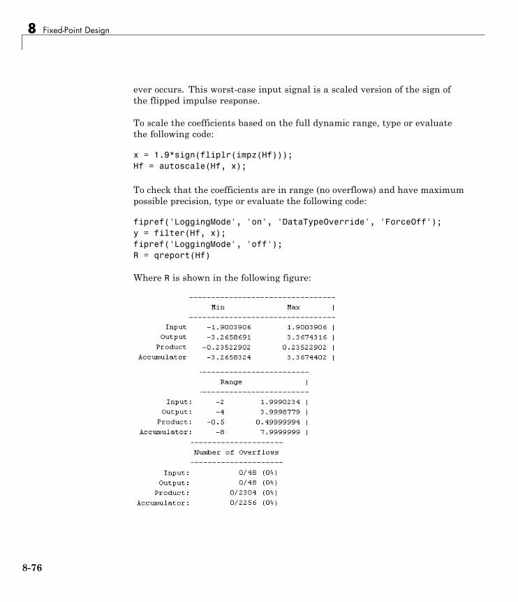
8 Fixed-Point Design
ever occurs. This worst-case input signal is a scaled version of the sign ofthe flipped impulse response.
To scale the coefficients based on the full dynamic range, type or evaluatethe following code:
x = 1.9*sign(fliplr(impz(Hf)));Hf = autoscale(Hf, x);
To check that the coefficients are in range (no overflows) and have maximumpossible precision, type or evaluate the following code:
fipref('LoggingMode', 'on', 'DataTypeOverride', 'ForceOff');y = filter(Hf, x);fipref('LoggingMode', 'off');R = qreport(Hf)
Where R is shown in the following figure:
8-76
Fixed-Point Filter Design
The report shows no overflows, and all data falls within the designed range.The conversion has completed successfully.
Compare Magnitude Response and Magnitude ResponseEstimateYou can use the fvtool GUI to analysis on your quantized filter, to see theeffects of the quantization on stopband attenuation, etc. Two importantlast checks when analyzing a quantized filter are the Magnitude ResponseEstimate and the Round-off Noise Power Spectrum. The value of theMagnitude Response Estimate analysis can be seen in the following example.
View the Magnitude Response Estimate
Begin by designing a simple lowpass filter using the command.
h = design(fdesign.lowpass, 'butter','SOSScaleNorm','Linf');
Now set the arithmetic to fixed-point.
h.arithmetic = 'fixed';
Open the filter using fvtool.
fvtool(h)
When fvtool displays the filter using the Magnitude response view, thequantized filter seems to match the original filter quite well.
8-77

8 Fixed-Point Design
However if you look at the Magnitude Response Estimate plot from theAnalysis menu, you will see that the actual filter created may not performnearly as well as indicated by the Magnitude Response plot.
8-78

Fixed-Point Filter Design
This is because by using the noise-based method of theMagnitude ResponseEstimate, you estimate the complex frequency response for your filter asdetermined by applying a noise- like signal to the filter input. MagnitudeResponse Estimate uses the Monte Carlo trials to generate a noise signalthat contains complete frequency content across the range 0 to Fs. For moreinformation about analyzing filters in this way, refer to the section titledAnalyzing Filters with a Noise-Based Method in the User Guide.
For more information, refer to McClellan, et al., Computer-Based Exercisesfor Signal Processing Using MATLAB 5, Prentice-Hall, 1998. See Project 5:Quantization Noise in Digital Filters, page 231.
8-79
8 Fixed-Point Design
Create an FIR Filter Using Integer Coefficients
Review of Fixed-Point Numbers
Terminology of Fixed-Point Numbers. DSP System Toolbox functionsassume fixed-point quantities are represented in two’s complement format,and are described using the WordLength and FracLength parameters. It iscommon to represent fractional quantities of WordLength 16 with the leftmostbit representing the sign and the remaining bits representing the fractionto the right of the binary point. Often the FracLength is thought of as thenumber of bits to the right of the binary point. However, there is a problemwith this interpretation when the FracLength is larger than the WordLength,or when the FracLength is negative.
To work around these cases, you can use the following interpretation of afixed-point quantity:
The register has a WordLength of B, or in other words it has B bits. The bitsare numbered from left to right from 0 to B-1. The most significant bit (MSB)is the leftmost bit, bB-1. The least significant bit is the right-most bit, b0. Youcan think of the FracLength as a quantity specifying how to interpret the bitsstored and resolve the value they represent. The value represented by the bitsis determined by assigning a weight to each bit:
In this figure, L is the integer FracLength. It can assume any value,depending on the quantization step size. L is necessary to interpret the valuethat the bits represent. This value is given by the equation
8-80

Fixed-Point Filter Design
value b bBB L
kk L
k
B= − +−
− − −
=
−
∑11
0
22 2
.
The value 2–L is the smallest possible difference between two numbersrepresented in this format, otherwise known as the quantization step. Inthis way, it is preferable to think of the FracLength as the negative ofthe exponent used to weigh the right-most, or least-significant, bit of thefixed-point number.
To reduce the number of bits used to represent a given quantity, you candiscard the least-significant bits. This method minimizes the quantizationerror since the bits you are removing carry the least weight. For instance, thefollowing figure illustrates reducing the number of bits from 4 to 2:
This means that the FracLength has changed from L to L – 2.
You can think of integers as being represented with a FracLength of L = 0, sothat the quantization step becomes .
Suppose B = 16 and L = 0. Then the numbers that can be represented are the
integers { , ,..., , , ..., , }− − −32768 32767 1 0 1 32766 32767 .
If you need to quantize these numbers to use only 8 bits to representthem, you will want to discard the LSBs as mentioned above, so that B=8and L = 0–8 = –8. The increments, or quantization step then becomes
2 2 2568 8− − = =( ) . So you will still have the same range of values, butwith less precision, and the numbers that can be represented become
{ , ,..., , , ,... , }− − −32768 32512 256 0 256 32256 32512 .
8-81
8 Fixed-Point Design
With this quantization the largest possible error becomes about 256/2 whenrounding to the nearest, with a special case for 32767.
Integers and Fixed-Point FiltersThis section provides an example of how you can create a filter with integercoefficients. In this example, a raised-cosine filter with floating-pointcoefficients is created, and the filter coefficients are then converted to integers.
Define the Filter Coefficients. To illustrate the concepts of using integerswith fixed-point filters, this example will use a raised-cosine filter:
b = rcosdesign(.25, 12.5, 8, 'sqrt');
The coefficients of b are normalized so that the passband gain is equal to 1,and are all smaller than 1. In order to make them integers, they will need tobe scaled. If you wanted to scale them to use 18 bits for each coefficient, therange of possible values for the coefficients becomes:
[ , ] [ , ]− − == −−2 2 1 131072 13107117 17
Because the largest coefficient of b is positive, it will need to be scaled as closeas possible to 131071 (without overflowing) in order to minimize quantizationerror. You can determine the exponent of the scale factor by executing:
B = 18; % Number of bits
L = floor(log2((2^(B-1)-1)/max(b))); % Round towards zero to avoid overflow
bsc = b*2^L;
Alternatively, you can use the fixed-point numbers autoscaling tool as follows:
bq = fi(b, true, B); % signed = true, B = 18 bitsL = bq.FractionLength;
It is a coincidence that B and L are both 18 in this case, because of the valueof the largest coefficient of b. If, for example, the maximum value of b were0.124, L would be 20 while B (the number of bits) would remain 18.
Build the FIR Filter. First create the filter using the direct form, tappeddelay line structure:
8-82

Fixed-Point Filter Design
h = dfilt.dffir(bsc);
In order to set the required parameters, the arithmetic must be set tofixed-point:
h.Arithmetic = 'fixed';h.CoeffWordLength = 18;
You can check that the coefficients of h are all integers:
all(h.Numerator == round(h.Numerator))
ans =
1
Now you can examine the magnitude response of the filter using fvtool:
fvtool(h, 'Color', 'white')
8-83
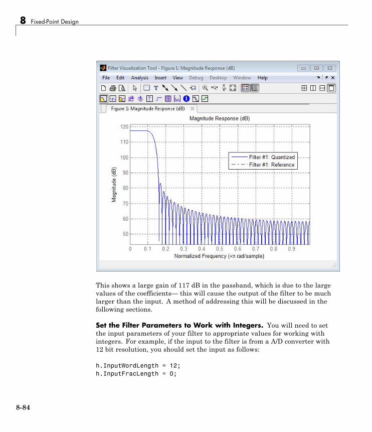
8 Fixed-Point Design
This shows a large gain of 117 dB in the passband, which is due to the largevalues of the coefficients— this will cause the output of the filter to be muchlarger than the input. A method of addressing this will be discussed in thefollowing sections.
Set the Filter Parameters to Work with Integers. You will need to setthe input parameters of your filter to appropriate values for working withintegers. For example, if the input to the filter is from a A/D converter with12 bit resolution, you should set the input as follows:
h.InputWordLength = 12;h.InputFracLength = 0;
8-84

Fixed-Point Filter Design
The info method returns a summary of the filter settings.
info(h)
Discrete-Time FIR Filter (real)
-------------------------------
Filter Structure : Direct-Form FIR
Filter Length : 101
Stable : Yes
Linear Phase : Yes (Type 1)
Arithmetic : fixed
Numerator : s18,0 -> [-131072 131072)
Input : s12,0 -> [-2048 2048)
Filter Internals : Full Precision
Output : s31,0 -> [-1073741824 1073741824) (auto determined)
Product : s29,0 -> [-268435456 268435456) (auto determined)
Accumulator : s31,0 -> [-1073741824 1073741824) (auto determined)
Round Mode : No rounding
Overflow Mode : No overflow
In this case, all the fractional lengths are now set to zero, meaning that thefilter h is set up to handle integers.
Create a Test Signal for the Filter. You can generate an input signal for thefilter by quantizing to 12 bits using the autoscaling feature, or you can followthe same procedure that was used for the coefficients, discussed previously.In this example, create a signal with two sinusoids:
n = 0:999;f1 = 0.1*pi; % Normalized frequency of first sinusoidf2 = 0.8*pi; % Normalized frequency of second sinusoidx = 0.9*sin(0.1*pi*n) + 0.9*sin(0.8*pi*n);xq = fi(x, true, 12); % signed = true, B = 12xsc = fi(xq.int, true, 12, 0);
Filter the Test Signal. To filter the input signal generated above, enterthe following:
ysc = filter(h, xsc);
8-85
8 Fixed-Point Design
Here ysc is a full precision output, meaning that no bits have been discardedin the computation. This makes ysc the best possible output you can achievegiven the 12–bit input and the 18–bit coefficients. This can be verified byfiltering using double-precision floating-point and comparing the results ofthe two filtering operations:
hd = double(h);xd = double(xsc);yd = filter(hd, xd);norm(yd-double(ysc))
ans =
0
Now you can examine the output compared to the input. This example isplotting only the last few samples to minimize the effect of transients:
idx = 800:950;xscext = double(xsc(idx)');gd = grpdelay(h, [f1 f2]);yidx = idx + gd(1);yscext = double(ysc(yidx)');stem(n(idx)', [xscext, yscext]);axis([800 950 -2.5e8 2.5e8]);legend('input', 'output');set(gcf, 'color', 'white');
8-86
Fixed-Point Filter Design
It is difficult to compare the two signals in this figure because of the largedifference in scales. This is due to the large gain of the filter, so you willneed to compensate for the filter gain:
stem(n(idx)', [2^18*xscext, yscext]);axis([800 950 -5e8 5e8]);legend('scaled input', 'output');
8-87
8 Fixed-Point Design
You can see how the signals compare much more easily once the scaling hasbeen done, as seen in the above figure.
Truncate the Output WordLength. If you examine the output wordlength,
ysc.WordLength
ans =
31
you will notice that the number of bits in the output is considerably greaterthan in the input. Because such growth in the number of bits representingthe data may not be desirable, you may need to truncate the wordlength ofthe output. As discussed in “Terminology of Fixed-Point Numbers” on page8-80the best way to do this is to discard the least significant bits, in orderto minimize error. However, if you know there are unused high order bits,you should discard those bits as well.
8-88
Fixed-Point Filter Design
To determine if there are unused most significant bits (MSBs), you can look atwhere the growth in WordLength arises in the computation. In this case, thebit growth occurs to accommodate the results of adding products of the input(12 bits) and the coefficients (18 bits). Each of these products is 29 bits long(you can verify this using info(h)). The bit growth due to the accumulation ofthe product depends on the filter length and the coefficient values- however,this is a worst-case determination in the sense that no assumption on theinput signal is made besides, and as a result there may be unused MSBs. Youwill have to be careful though, as MSBs that are deemed unused incorrectlywill cause overflows.
Suppose you want to keep 16 bits for the output. In this case, there is nobit-growth due to the additions, so the output bit setting will be 16 for thewordlength and –14 for the fraction length.
Since the filtering has already been done, you can discard some bits from ysc:
yout = fi(ysc, true, 16, -14);
Alternatively, you can set the filter output bit lengths directly (this is useful ifyou plan on filtering many signals):
specifyall(h);h.OutputWordLength = 16;h.OutputFracLength = -14;yout2 = filter(h, xsc);
You can verify that the results are the same either way:
norm(double(yout) - double(yout2))
ans =
0
However, if you compare this to the full precision output, you will notice thatthere is rounding error due to the discarded bits:
norm(double(yout)-double(ysc))
8-89
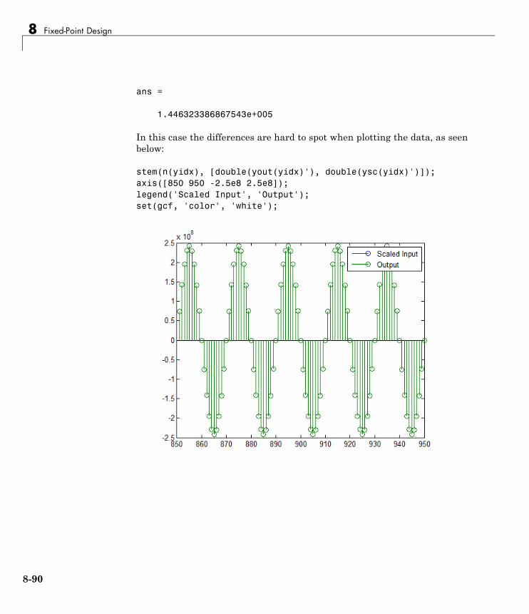
8 Fixed-Point Design
ans =
1.446323386867543e+005
In this case the differences are hard to spot when plotting the data, as seenbelow:
stem(n(yidx), [double(yout(yidx)'), double(ysc(yidx)')]);axis([850 950 -2.5e8 2.5e8]);legend('Scaled Input', 'Output');set(gcf, 'color', 'white');
8-90
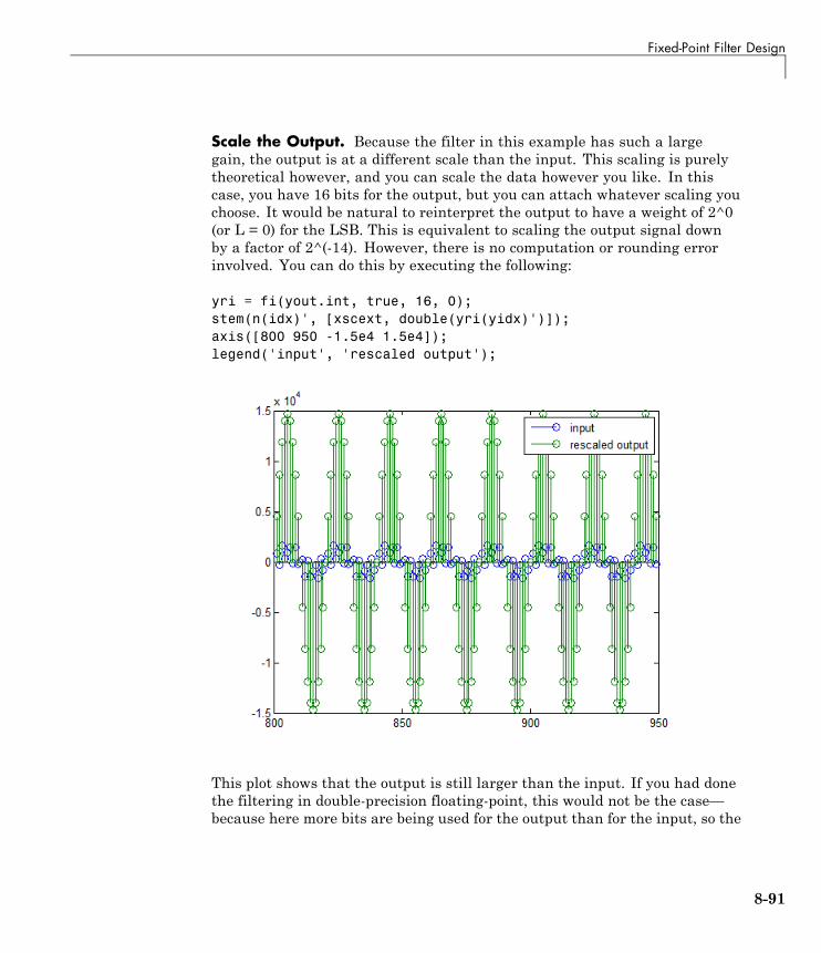
Fixed-Point Filter Design
Scale the Output. Because the filter in this example has such a largegain, the output is at a different scale than the input. This scaling is purelytheoretical however, and you can scale the data however you like. In thiscase, you have 16 bits for the output, but you can attach whatever scaling youchoose. It would be natural to reinterpret the output to have a weight of 2^0(or L = 0) for the LSB. This is equivalent to scaling the output signal downby a factor of 2^(-14). However, there is no computation or rounding errorinvolved. You can do this by executing the following:
yri = fi(yout.int, true, 16, 0);stem(n(idx)', [xscext, double(yri(yidx)')]);axis([800 950 -1.5e4 1.5e4]);legend('input', 'rescaled output');
This plot shows that the output is still larger than the input. If you had donethe filtering in double-precision floating-point, this would not be the case—because here more bits are being used for the output than for the input, so the
8-91
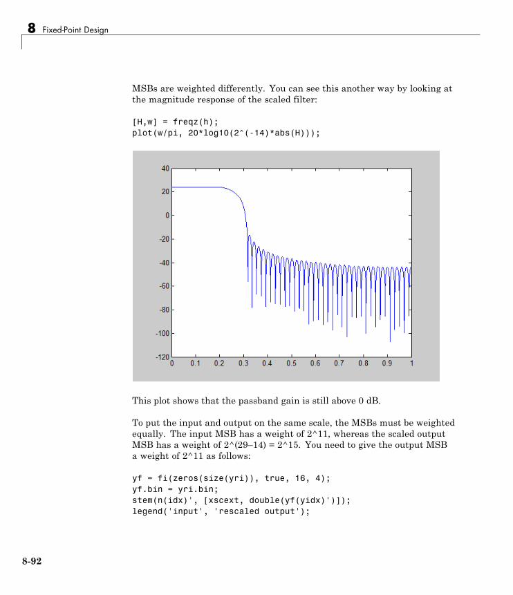
8 Fixed-Point Design
MSBs are weighted differently. You can see this another way by looking atthe magnitude response of the scaled filter:
[H,w] = freqz(h);plot(w/pi, 20*log10(2^(-14)*abs(H)));
This plot shows that the passband gain is still above 0 dB.
To put the input and output on the same scale, the MSBs must be weightedequally. The input MSB has a weight of 2^11, whereas the scaled outputMSB has a weight of 2^(29–14) = 2^15. You need to give the output MSBa weight of 2^11 as follows:
yf = fi(zeros(size(yri)), true, 16, 4);yf.bin = yri.bin;stem(n(idx)', [xscext, double(yf(yidx)')]);legend('input', 'rescaled output');
8-92
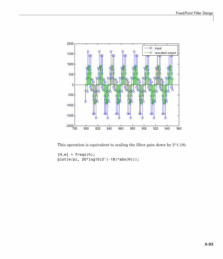
Fixed-Point Filter Design
This operation is equivalent to scaling the filter gain down by 2^(-18).
[H,w] = freqz(h);plot(w/pi, 20*log10(2^(-18)*abs(H)));
8-93

8 Fixed-Point Design
The above plot shows a 0 dB gain in the passband, as desired.
With this final version of the output, yf is no longer an integer. However thisis only due to the interpretation- the integers represented by the bits in yfare identical to the ones represented by the bits in yri. You can verify thisby comparing them:
max(abs(yf.int - yri.int))
ans =
0
8-94

Fixed-Point Filter Design
Configure Filter Parameters to Work with Integers Using theset2int Method
• “Set the Filter Parameters to Work with Integers” on page 8-95
• “Reinterpret the Output” on page 8-96
Set the Filter Parameters to Work with Integers. The set2int methodprovides a convenient way of setting filter parameters to work with integers.The method works by scaling the coefficients to integer numbers, and settingthe coefficients and input fraction length to zero. This makes it possible foryou to use floating-point coefficients directly.
h = dfilt.dffir(b);h.Arithmetic = 'fixed';
The coefficients are represented with 18 bits and the input signal isrepresented with 12 bits:
g = set2int(h, 18, 12);g_dB = 20*log10(g)
g_dB =
1.083707984390332e+002
The set2int method returns the gain of the filter by scaling the coefficientsto integers, so the gain is always a power of 2. You can verify that the gain weget here is consistent with the gain of the filter previously. Now you can alsocheck that the filter h is set up properly to work with integers:
info(h)
Discrete-Time FIR Filter (real)
-------------------------------
Filter Structure : Direct-Form FIR
Filter Length : 101
Stable : Yes
Linear Phase : Yes (Type 1)
Arithmetic : fixed
Numerator : s18,0 -> [-131072 131072)
8-95

8 Fixed-Point Design
Input : s12,0 -> [-2048 2048)
Filter Internals : Full Precision
Output : s31,0 -> [-1073741824 1073741824) (auto determined)
Product : s29,0 -> [-268435456 268435456) (auto determined)
Accumulator: s31,0 -> [-1073741824 1073741824) (auto determined)
Round Mode : No rounding
Overflow Mode : No overflow
Here you can see that all fractional lengths are now set to zero, so this filter isset up properly for working with integers.
Reinterpret the Output. You can compare the output to the double-precisionfloating-point reference output, and verify that the computation done by thefilter h is done in full precision.
yint = filter(h, xsc);norm(yd - double(yint))
ans =
0
You can then truncate the output to only 16 bits:
yout = fi(yint, true, 16);stem(n(yidx), [xscext, double(yout(yidx)')]);axis([850 950 -2.5e8 2.5e8]);legend('input', 'output');
8-96

Fixed-Point Filter Design
Once again, the plot shows that the input and output are at different scales.In order to scale the output so that the signals can be compared more easilyin a plot, you will need to weigh the MSBs appropriately. You can computethe new fraction length using the gain of the filter when the coefficients wereinteger numbers:
WL = yout.WordLength;FL = yout.FractionLength + log2(g);yf2 = fi(zeros(size(yout)), true, WL, FL);yf2.bin = yout.bin;
stem(n(idx)', [xscext, double(yf2(yidx)')]);axis([800 950 -2e3 2e3]);legend('input', 'rescaled output');
8-97

8 Fixed-Point Design
This final plot shows the filtered data re-scaled to match the input scale.
Fixed-Point Filtering in Simulink
• “Fixed-Point Filtering Blocks” on page 8-98
• “Filter Implementation Blocks” on page 8-99
• “Filter Design and Implementation Blocks” on page 8-99
Fixed-Point Filtering BlocksThe following DSP System Toolbox blocks enable you to design and/or realizea variety of fixed-point filters:
• CIC Decimation
• CIC Interpolation
8-98

Fixed-Point Filter Design
• Digital Filter
• Filter Realization Wizard
• FIR Decimation
• FIR Interpolation
• Two-Channel Analysis Subband Filter
• Two-Channel Synthesis Subband Filter
Filter Implementation BlocksThe FIR Decimation, FIR Interpolation, Two-Channel Analysis SubbandFilter, Two-Channel Synthesis Subband Filter, and Digital Filter blocks areall implementation blocks. They allow you to implement filters for which youalready know the filter coefficients. The first four blocks each implementtheir respective filter type, while the Digital Filter block can create a varietyof filter structures. All filter structures supported by the Digital Filter blocksupport fixed-point signals.
Filter Design and Implementation BlocksThe Filter Realization Wizard block invokes part of the Filter Design andAnalysis Tool from Signal Processing Toolbox software. This block allows youboth to design new filters and to implement filters for which you alreadyknow the coefficients. In its implementation stage, the Filter RealizationWizard creates a filter realization using Sum, Gain, and Delay blocks. Youcan use this block to design and/or implement numerous types of fixed-pointand floating-point single-channel filters. See the Filter Realization Wizardreference page for more information about this block.
The CIC Decimation and CIC Interpolation blocks allow you to design andimplement Cascaded Integrator-Comb filters. See their block reference pagesfor more information.
8-99

8 Fixed-Point Design
8-100
9
Code Generation
Learn how to generate code for signal processing applications.
• “Understanding Code Generation” on page 9-2
• “Functions and System Objects Supported for Code Generation” on page 9-4
• “Generate Code from MATLAB” on page 9-12
• “Generate Code from Simulink” on page 9-13
• “How to Run a Generated Executable Outside MATLAB” on page 9-18
• “Verify FIR Filter on ARM Cortex-M Processor” on page 9-19
• “CMSIS Conditions for DSP System objects to Support ARM Cortex-M”on page 9-24
• “Fixed-Point Property Settings for dsp.FIRFilter” on page 9-31
• “Fixed-Point Property Settings for Discrete FIR Filter block” on page 9-32
• “CMSIS Conditions for DSP Blocks to Support ARM Cortex-M” on page 9-33
• “Support Packages and Support Package Installer” on page 9-41
• “Open Examples for This Support Package” on page 9-43
• “Install This Support Package on Other Computers” on page 9-47
• “Supported CMSIS Functions for ARM® Cortex®-M Processors” on page9-49
9 Code Generation
Understanding Code Generation
In this section...
“Code Generation with the Simulink® Coder™ Product” on page 9-2
“Highly Optimized Generated ANSI C Code” on page 9-3
Code Generation with the Simulink Coder ProductYou can use the DSP System Toolbox, Simulink Coder, and Embedded Coder®
products together to generate code that you can use to implement your modelfor a practical application. For instance, you can create an executable fromyour Simulink model to run on a target chip.
This chapter introduces you to the basic concepts of code generation usingthese tools.
Shared Library DependenciesIn general, the code you generate from DSP System Toolbox blocks is portableANSI C code. After you generate the code, you can deploy it on anothermachine. For more information on how to do so, see “Relocate Code to AnotherDevelopment Environment” in the Simulink Coder documentation.
There are a few DSP System Toolbox blocks that generate code with limitedportability. These blocks use precompiled shared libraries, such as DLLs, tosupport I/O for specific types of devices and file formats. To find out whichblocks use precompiled shared libraries, open the DSP System Toolbox BlockSupport Table. You can identify blocks that use precompiled shared librariesby checking the footnotes listed in the Code Generation Support column ofthe table. All blocks that use shared libraries have the following footnote:
Host computer only. Excludes Real-Time Windows (RTWIN) target.
Simulink Coder provides functions to help you set up and manage the buildinformation for your models. For example, one of the functions that SimulinkCoder provides is getNonBuildFiles. This function allows you to identify theshared libraries required by blocks in your model. If your model contains anyblocks that use precompiled shared libraries, you can install those libraries
9-2

Understanding Code Generation
on the target system. The folder that you install the shared libraries in mustbe on the system path. The target system does not need to have MATLABinstalled, but it does need to be supported by MATLAB.
Highly Optimized Generated ANSI C CodeAll DSP System Toolbox blocks generate highly optimized ANSI C code. ThisC code is often suitable for embedded applications, and includes the followingoptimizations:
• Function reuse (run-time libraries) — The generated code reusescommon algorithmic functions via calls to shared utility functions.Shared utility functions are highly optimized ANSI/ISO C functions thatimplement core algorithms such as FFT and convolution.
• Parameter reuse (Simulink Coder run-time parameters)— In manycases, if there are multiple instances of a block that all have the same valuefor a specific parameter, each block instance points to the same variable inthe generated code. This process reduces memory requirements.
• Blocks have parameters that affect code optimization — Someblocks, such as the Sine Wave block, have parameters that enable youto optimize the simulation for memory or for speed. These optimizationsalso apply to code generation.
• Other optimizations — Use of contiguous input and output arrays,reusable inputs, overwritable arrays, and inlined algorithms providesmaller generated C code that is more efficient at run time.
9-3
9 Code Generation
Functions and System Objects Supported for CodeGeneration
If you have a MATLAB Coder license, you can generate C and C++ code fromMATLAB code that contains DSP System Toolbox functions and Systemobjects. For more information about C and C++ code generation fromMATLAB code, see the MATLAB Coder documentation. For more informationabout generating code from System objects, see “System Objects in MATLABCode Generation”.
The following DSP System Toolbox functions and System objects aresupported for C and C++ code generation from MATLAB code.
Name Remarks and Limitations
Estimation
dsp.BurgAREstimator “System Objects in MATLAB Code Generation”
dsp.BurgSpectrumEstimator “System Objects in MATLAB Code Generation”
dsp.CepstralToLPC “System Objects in MATLAB Code Generation”
dsp.CrossSpectrumEstimator “System Objects in MATLAB Code Generation”
dsp.LevinsonSolver “System Objects in MATLAB Code Generation”
dsp.LPCToAutocorrelation “System Objects in MATLAB Code Generation”
dsp.LPCToCepstral “System Objects in MATLAB Code Generation”
dsp.LPCToLSF “System Objects in MATLAB Code Generation”
dsp.LPCToLSP “System Objects in MATLAB Code Generation”
dsp.LPCToRC “System Objects in MATLAB Code Generation”
dsp.LSFToLPC “System Objects in MATLAB Code Generation”
dsp.LSPToLPC “System Objects in MATLAB Code Generation”
dsp.RCToAutocorrelation “System Objects in MATLAB Code Generation”
dsp.RCToLPC “System Objects in MATLAB Code Generation”
dsp.SpectrumEstimator “System Objects in MATLAB Code Generation”
9-4

Functions and System Objects Supported for Code Generation
Name Remarks and Limitations
dsp.TransferFunctionEstimator “System Objects in MATLAB Code Generation”
Filters
ca2tf All inputs must be constant. Expressions orvariables are allowed if their values do notchange.
cl2tf All inputs must be constant. Expressions orvariables are allowed if their values do notchange.
dsp.AdaptiveLatticeFilter “System Objects in MATLAB Code Generation”
dsp.AffineProjectionFilter “System Objects in MATLAB Code Generation”
dsp.AllpoleFilter• “System Objects in MATLAB CodeGeneration”
• Only the Denominator property is tunablefor code generation.
dsp.BiquadFilter “System Objects in MATLAB Code Generation”
dsp.CICDecimator “System Objects in MATLAB Code Generation”
dsp.CICInterpolator “System Objects in MATLAB Code Generation”
dsp.DigitalFilter• “System Objects in MATLAB CodeGeneration”
• The SOSMatrix and Scalevalues propertiesare not supported for code generation.dsp.FastTransversalFilter “System Objects in MATLAB Code Generation”
dsp.FilteredXLMSFilter “System Objects in MATLAB Code Generation”
dsp.FIRDecimator “System Objects in MATLAB Code Generation”
9-5

9 Code Generation
Name Remarks and Limitations
dsp.FIRFilter• “System Objects in MATLAB CodeGeneration”
• Only the Numerator property is tunable forcode generation.
dsp.FIRInterpolator “System Objects in MATLAB Code Generation”
dsp.FIRRateConverter “System Objects in MATLAB Code Generation”
dsp.FrequencyDomainAdaptiveFilter “System Objects in MATLAB Code Generation”
dsp.IIRFilter• Only the Numerator and Denominatorproperties are tunable for code generation.
• “System Objects in MATLAB CodeGeneration”
dsp.KalmanFilter “System Objects in MATLAB Code Generation”
dsp.LMSFilter “System Objects in MATLAB Code Generation”
dsp.RLSFilter “System Objects in MATLAB Code Generation”
firceqrip All inputs must be constant. Expressions orvariables are allowed if their values do notchange.
fireqint All inputs must be constant. Expressions orvariables are allowed if their values do notchange.
firgr• All inputs must be constant. Expressions orvariables are allowed if their values do notchange.
• Does not support syntaxes that have cellarray input.
firhalfband All inputs must be constant. Expressions orvariables are allowed if their values do notchange.
9-6
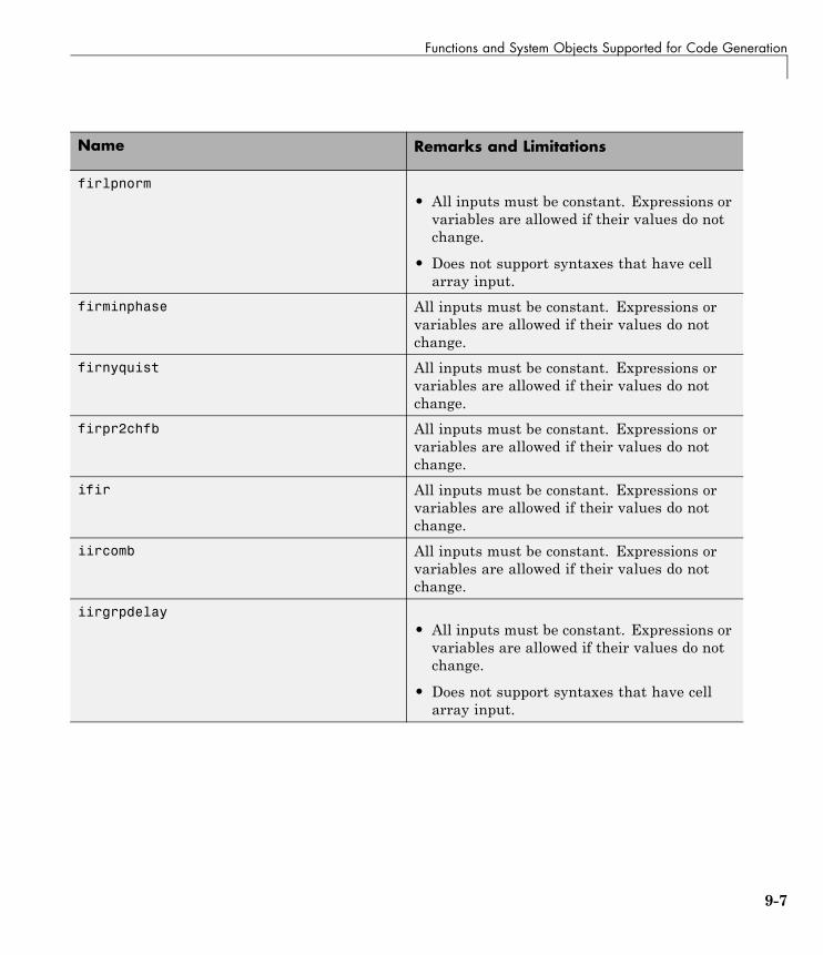
Functions and System Objects Supported for Code Generation
Name Remarks and Limitations
firlpnorm• All inputs must be constant. Expressions orvariables are allowed if their values do notchange.
• Does not support syntaxes that have cellarray input.
firminphase All inputs must be constant. Expressions orvariables are allowed if their values do notchange.
firnyquist All inputs must be constant. Expressions orvariables are allowed if their values do notchange.
firpr2chfb All inputs must be constant. Expressions orvariables are allowed if their values do notchange.
ifir All inputs must be constant. Expressions orvariables are allowed if their values do notchange.
iircomb All inputs must be constant. Expressions orvariables are allowed if their values do notchange.
iirgrpdelay• All inputs must be constant. Expressions orvariables are allowed if their values do notchange.
• Does not support syntaxes that have cellarray input.
9-7
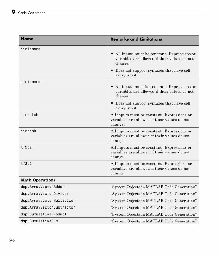
9 Code Generation
Name Remarks and Limitations
iirlpnorm• All inputs must be constant. Expressions orvariables are allowed if their values do notchange.
• Does not support syntaxes that have cellarray input.
iirlpnormc• All inputs must be constant. Expressions orvariables are allowed if their values do notchange.
• Does not support syntaxes that have cellarray input.
iirnotch All inputs must be constant. Expressions orvariables are allowed if their values do notchange.
iirpeak All inputs must be constant. Expressions orvariables are allowed if their values do notchange.
tf2ca All inputs must be constant. Expressions orvariables are allowed if their values do notchange.
tf2cl All inputs must be constant. Expressions orvariables are allowed if their values do notchange.
Math Operations
dsp.ArrayVectorAdder “System Objects in MATLAB Code Generation”
dsp.ArrayVectorDivider “System Objects in MATLAB Code Generation”
dsp.ArrayVectorMultiplier “System Objects in MATLAB Code Generation”
dsp.ArrayVectorSubtractor “System Objects in MATLAB Code Generation”
dsp.CumulativeProduct “System Objects in MATLAB Code Generation”
dsp.CumulativeSum “System Objects in MATLAB Code Generation”
9-8

Functions and System Objects Supported for Code Generation
Name Remarks and Limitations
dsp.LDLFactor “System Objects in MATLAB Code Generation”
dsp.LevinsonSolver “System Objects in MATLAB Code Generation”
dsp.LowerTriangularSolver “System Objects in MATLAB Code Generation”
dsp.LUFactor “System Objects in MATLAB Code Generation”
dsp.Normalizer “System Objects in MATLAB Code Generation”
dsp.UpperTriangularSolver “System Objects in MATLAB Code Generation”
Quantizers
dsp.ScalarQuantizerDecoder “System Objects in MATLAB Code Generation”
dsp.ScalarQuantizerEncoder “System Objects in MATLAB Code Generation”
dsp.VectorQuantizerDecoder “System Objects in MATLAB Code Generation”
dsp.VectorQuantizerEncoder “System Objects in MATLAB Code Generation”
Scopes
dsp.SpectrumAnalyzer This System object does not generate code. It isautomatically declared as an extrinsic variableusing the coder.extrinsic function.
dsp.TimeScope This System object does not generate code. It isautomatically declared as an extrinsic variableusing the coder.extrinsic function.
Signal Management
dsp.Counter “System Objects in MATLAB Code Generation”
dsp.DelayLine “System Objects in MATLAB Code Generation”
Signal Operations
dsp.Convolver “System Objects in MATLAB Code Generation”
dsp.DCBlocker “System Objects in MATLAB Code Generation”
dsp.Delay “System Objects in MATLAB Code Generation”
dsp.DigitalDownConverter “System Objects in MATLAB Code Generation”
dsp.DigitalUpConverter “System Objects in MATLAB Code Generation”
9-9

9 Code Generation
Name Remarks and Limitations
dsp.Interpolator “System Objects in MATLAB Code Generation”
dsp.NCO “System Objects in MATLAB Code Generation”
dsp.PeakFinder “System Objects in MATLAB Code Generation”
dsp.PhaseUnwrapper “System Objects in MATLAB Code Generation”
dsp.VariableFractionalDelay “System Objects in MATLAB Code Generation”
dsp.VariableIntegerDelay “System Objects in MATLAB Code Generation”
dsp.Window• This object has no tunable properties forcode generation.
• “System Objects in MATLAB CodeGeneration”
dsp.ZeroCrossingDetector “System Objects in MATLAB Code Generation”
Sinks
dsp.AudioPlayer “System Objects in MATLAB Code Generation”
dsp.AudioFileWriter “System Objects in MATLAB Code Generation”
dsp.UDPSender “System Objects in MATLAB Code Generation”
Sources
dsp.AudioFileReader “System Objects in MATLAB Code Generation”
dsp.AudioRecorder “System Objects in MATLAB Code Generation”
dsp.SignalSource “System Objects in MATLAB Code Generation”
dsp.SineWave• This object has no tunable properties forcode generation.
• “System Objects in MATLAB CodeGeneration”
dsp.UDPReceiver “System Objects in MATLAB Code Generation”
Statistics
9-10
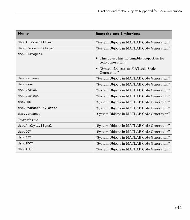
Functions and System Objects Supported for Code Generation
Name Remarks and Limitations
dsp.Autocorrelator “System Objects in MATLAB Code Generation”
dsp.Crosscorrelator “System Objects in MATLAB Code Generation”
dsp.Histogram• This object has no tunable properties forcode generation.
• “System Objects in MATLAB CodeGeneration”
dsp.Maximum “System Objects in MATLAB Code Generation”
dsp.Mean “System Objects in MATLAB Code Generation”
dsp.Median “System Objects in MATLAB Code Generation”
dsp.Minimum “System Objects in MATLAB Code Generation”
dsp.RMS “System Objects in MATLAB Code Generation”
dsp.StandardDeviation “System Objects in MATLAB Code Generation”
dsp.Variance “System Objects in MATLAB Code Generation”
Transforms
dsp.AnalyticSignal “System Objects in MATLAB Code Generation”
dsp.DCT “System Objects in MATLAB Code Generation”
dsp.FFT “System Objects in MATLAB Code Generation”
dsp.IDCT “System Objects in MATLAB Code Generation”
dsp.IFFT “System Objects in MATLAB Code Generation”
9-11

9 Code Generation
Generate Code from MATLABWhen you have a license for the MATLAB Coder product, you can generatestandalone C and C++ from MATLAB code. See the MATLAB Coderdocumentation for details on supported functionality and workflow.
9-12

Generate Code from Simulink®
Generate Code from Simulink
In this section...
“Open and Run the Model” on page 9-13
“Generate Code from the Model” on page 9-15
“Build and Run the Generated Code” on page 9-15
Note You must have both the DSP System Toolbox and Simulink Coderproducts installed on your computer to complete the procedures in this section.
Open and Run the ModelThe ex_codegen_dsp model implements a simple adaptive filter to removenoise from a signal while simultaneously identifying a filter that characterizesthe noise frequency content. To open this model, enter
open_system('ex_codegen_dsp')
9-13

9 Code Generation
Run the model and observe the output in both scopes. This model saves thefilter weights each time they adapt. You can plot the last set of coefficientsusing the following command:
plot(filter_wts(:,:,1201))
9-14

Generate Code from Simulink®
Generate Code from the ModelTo generate code from the model, you must first ensure that you have writepermission in your current folder. The code generation process creates a newsubfolder inside the current MATLAB working folder. MATLAB saves all ofthe files created by the code generation process in that subfolder, includingthose which contain the generated C source code.
To start the code generation process, click the Incremental build icon ( )on your model toolbar. After the model finishes generating code, the CodeGeneration Report appears, allowing you to inspect the generated code.You may also notice that the build process created a new subfolder insideof your current MATLAB working folder. The name of this folder consistsof the model name, followed by the suffix _grt_rtw. In the case of thisexample, the subfolder that contains the generated C source code is namedex_codegen_dsp_grt_rtw.
Build and Run the Generated Code
Setup the C/C++ CompilerIf you want to build and run the generated code, you needto have access to a C compiler. For more information aboutwhich compilers are supported in the current release, seehttp://www.mathworks.com/support/compilers/current_release/.
To setup your compiler, run the following command:
mex setup
Build the Generated CodeAfter your compiler is setup, you can build and run the generated code. Theex_codegen_dsp model is currently configured to generate code only. To buildthe generated code, you must first make the following changes:
1 Open the Model Configuration Parameters dialog, navigate to theCode Generation tab, and clear the Generate Code Only checkbox.
2 Click OK to apply your changes and close the dialog box.
9-15
9 Code Generation
3 From the model toolbar, click the Incremental build icon ( ).
Because you re-configured the model to generate and build code, the codegeneration process continues until the code is compiled and linked.
Run the Generated CodeTo run the generated code, enter the following command at the MATLABprompt:
!ex_codegen_dsp
Running the generated code creates a MAT-file which contains the samevariables as those generated by simulating the model. The variables in theMAT-file are named with a prefix of rt_. After you run the generated code,you can load the variables from the MAT-file by typing the following commandat the MATLAB prompt:
load ex_codegen_dsp.mat
You can now compare the variables from the generated code with thevariables from the model simulation. To plot the last set of coefficients fromthe generated code, enter the following command at the MATLAB prompt:
plot(rt_filter_wts(:,:,1201))
The last set of coefficients from the generated code are shown in the followingfigure.
9-16

Generate Code from Simulink®
For further information on generating code from Simulink, see the “SimulinkCoder” documentation.
9-17

9 Code Generation
How to Run a Generated Executable Outside MATLABTo run your generated standalone executable application in Shell, you need toset the environment variables as follows:
Platform Command
Mac setenv DYLD_LIBRARY_PATH$DYLD_LIBRARY_PATH:$MATLABROOT/bin/maci64(csh/tcsh)exportDYLD_LIBRARY_PATH$DYLD_LIBRARY_PATH:$MATLABROOT/bin/maci64 (Bash)
Linux setenv LD_LIBRARY_PATH$LD_LIBRARY_PATH:$MATLABROOT/bin/glnxa64(csh/tcsh)exportLD_LIBRARY_PATH$LD_LIBRARY_PATH:$MATLABROOT/bin/glnxa64 (Bash)
Windows set PATH =$MATLABROOT\bin\win32;%PATH%set PATH =$MATLABROOT\bin\win64;%PATH%
9-18
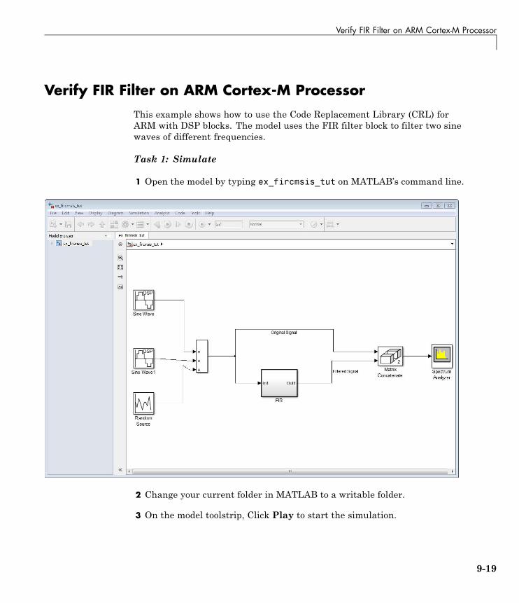
Verify FIR Filter on ARM Cortex-M Processor
Verify FIR Filter on ARM Cortex-M ProcessorThis example shows how to use the Code Replacement Library (CRL) forARM with DSP blocks. The model uses the FIR filter block to filter two sinewaves of different frequencies.
Task 1: Simulate
1 Open the model by typing ex_fircmsis_tut on MATLAB’s command line.
2 Change your current folder in MATLAB to a writable folder.
3 On the model toolstrip, Click Play to start the simulation.
9-19

9 Code Generation
4 Click Stop to end simulation.
Task 2: Setup model for Code Replacement
1 Under Simulation, click Model Configuration Parameters to openthe dialog box.
2 Select Code Generation category.
3 Set the System target file to ert.tlc, and select Generate code only.
4 Select Interface under the Code Generation category.
9-20

Verify FIR Filter on ARM Cortex-M Processor
5 Set Code replacement library to ARM Cortex-M.
Task 3: Generate code
1 Right-click the FIR subsystem. From the drop-down menu that opens,choose C/C++ Code > Build This Subsystem. When the Build code forSubsystem dialog box opens, Click Build to start generating code.
9-21

9 Code Generation
2 When build finishes processing, a code generation report comes up.
3 Click on the FIR.c file. Notice the CMSIS function; arm_fir_init_f32 callin the initialize function (FIR_initialize). Also, notice the CMSIS function;arm_fir_f32 in the model step function (FIR_step).
9-22

Verify FIR Filter on ARM Cortex-M Processor
Task 4: Use Processor in the Loop (PIL)
To perform the previous steps using PIL, you need to have the EmbededCoder Support Package for ARM Cortex-M Processors, and the DST SupportPackage for ARM Cortex-M Processors. The following examples shows youhow to use PIL with ARM Cortex-M:
• Code Verification and Validation with PIL and External Mode
• Code Optimization Using CMSIS DSP Library
For instructions on accessing these examples, see: “Open Examples for ThisSupport Package” on page 9-43.
9-23

9 Code Generation
CMSIS Conditions for DSP System objects to Support ARMCortex-M
In this section...
“General Conditions on All System objects” on page 9-24
“Specific System object properties Used to support CMSIS” on page 9-24
General Conditions on All System objectsUnder the following conditions, CMSIS support for DSP System objects isavailable:
• Input data type is single. (except for dsp.FIRFilter with 'Direct Form'Structure, where both single and fixed-point data types are supported.)
• Input or output is real. (Support for complex input or output is availablefor dsp.FFT and dsp.IFFT System objects.)
• Input is single channel.
Note In the Fixed-point mode of the CMSIS DSP (FIR) function, Wrap isused for intermediate MAC operations if accumulator result overflows. At theend, the accumulator is right shifted and saturated to the output data type.For discrete FIR block or system object, there is only one overflow settingfor accumulator and output. So if overflow happens in accumulation, thesimulation result will not match the CMSIS library result.
Specific System object properties Used to supportCMSISDSP System objects supporting the ARM-Cortex-M package require a set ofconditions that would allow code replacement with the CMSIS Library, whengenerating C code from a model or from MATLAB code. The CMSIS librarysupports these DSP System objects only when you set specific properties, asindicated in the following table. To use the CMSIS library with these Systemobjects offering ARM support, you must follow these rules for specifyingproperties.
9-24
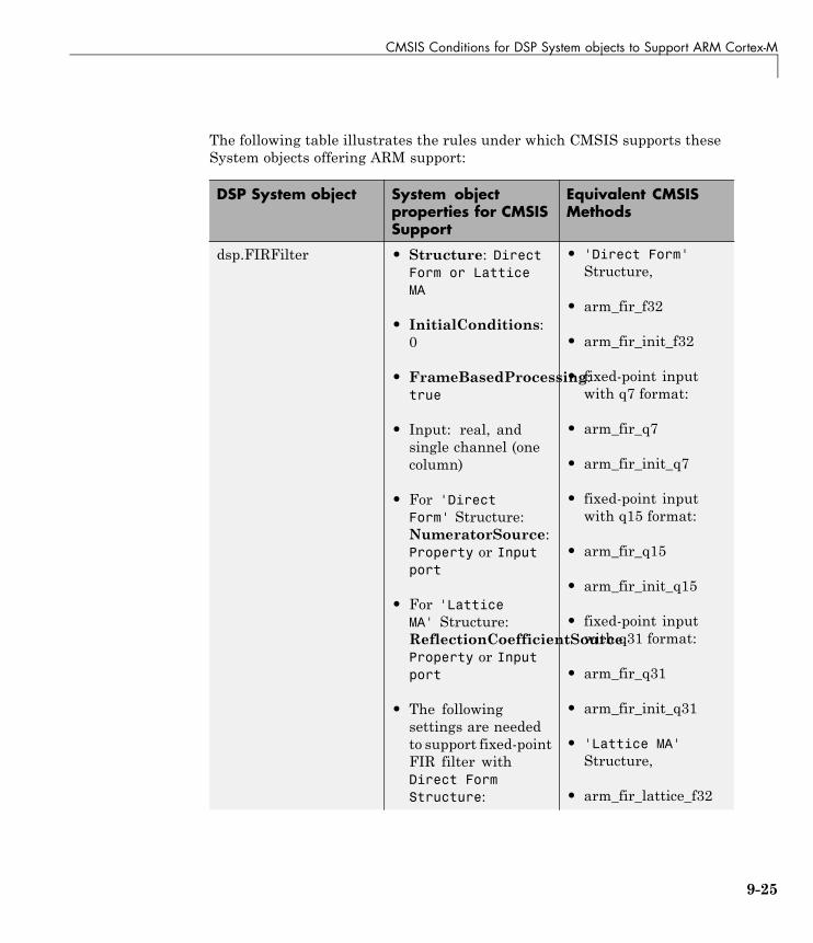
CMSIS Conditions for DSP System objects to Support ARM Cortex-M
The following table illustrates the rules under which CMSIS supports theseSystem objects offering ARM support:
DSP System object System objectproperties for CMSISSupport
Equivalent CMSISMethods
dsp.FIRFilter • Structure: DirectForm or LatticeMA
• InitialConditions:0
• FrameBasedProcessing:true
• Input: real, andsingle channel (onecolumn)
• For 'DirectForm' Structure:NumeratorSource:Property or Inputport
• For 'LatticeMA' Structure:ReflectionCoefficientSource:Property or Inputport
• The followingsettings are neededto support fixed-pointFIR filter withDirect FormStructure:
• 'Direct Form'Structure,
• arm_fir_f32
• arm_fir_init_f32
• fixed-point inputwith q7 format:
• arm_fir_q7
• arm_fir_init_q7
• fixed-point inputwith q15 format:
• arm_fir_q15
• arm_fir_init_q15
• fixed-point inputwith q31 format:
• arm_fir_q31
• arm_fir_init_q31
• 'Lattice MA'Structure,
• arm_fir_lattice_f32
9-25
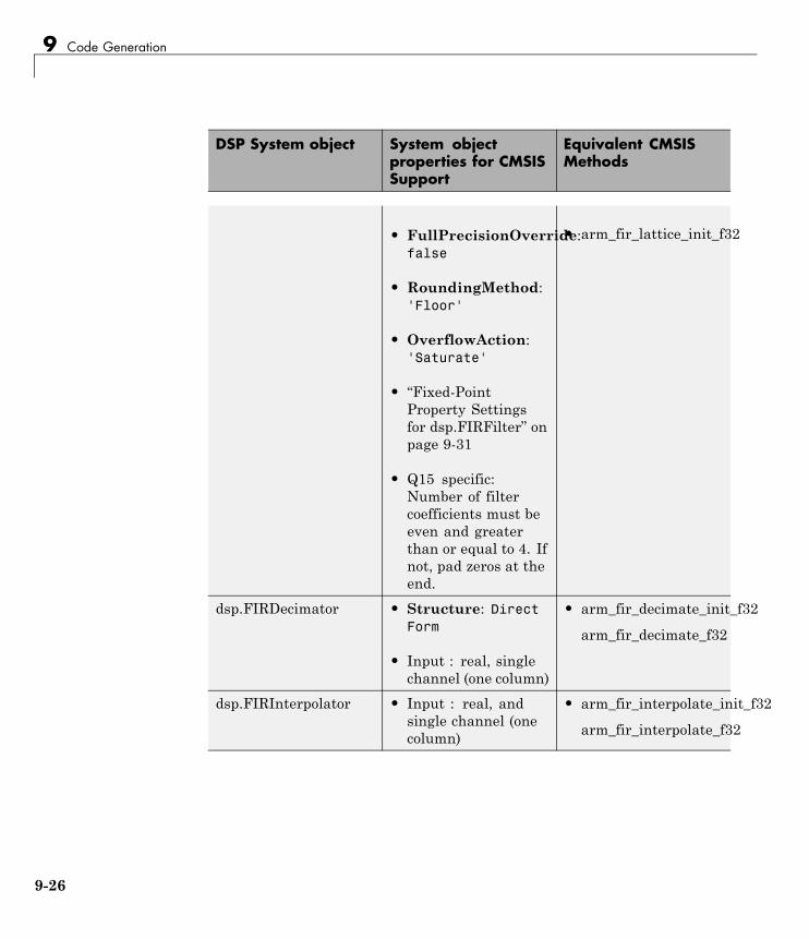
9 Code Generation
DSP System object System objectproperties for CMSISSupport
Equivalent CMSISMethods
• FullPrecisionOverride:false
• RoundingMethod:'Floor'
• OverflowAction:'Saturate'
• “Fixed-PointProperty Settingsfor dsp.FIRFilter” onpage 9-31
• Q15 specific:Number of filtercoefficients must beeven and greaterthan or equal to 4. Ifnot, pad zeros at theend.
• arm_fir_lattice_init_f32
dsp.FIRDecimator • Structure: DirectForm
• Input : real, singlechannel (one column)
• arm_fir_decimate_init_f32
arm_fir_decimate_f32
dsp.FIRInterpolator • Input : real, andsingle channel (onecolumn)
• arm_fir_interpolate_init_f32
arm_fir_interpolate_f32
9-26
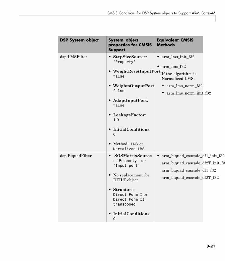
CMSIS Conditions for DSP System objects to Support ARM Cortex-M
DSP System object System objectproperties for CMSISSupport
Equivalent CMSISMethods
dsp.LMSFilter • StepSizeSource:'Property'
• WeightResetInputPort:false
• WeightsOutputPort:false
• AdaptInputPort:false
• LeakageFactor:1.0
• InitialConditions:0
• Method: LMS orNormalized LMS
• arm_lms_init_f32
• arm_lms_f32
If the algorithm isNormalized LMS:
- arm_lms_norm_f32
- arm_lms_norm_init_f32
dsp.BiquadFilter • SOSMatrixSource: 'Property' or'Input port'
• No replacement forDFILT object
• Structure:Direct Form I orDirect Form IItransposed
• InitialConditions:0
• arm_biquad_cascade_df1_init_f32
arm_biquad_cascade_df2T_init_f3
arm_biquad_cascade_df1_f32
arm_biquad_cascade_df2T_f32
9-27

9 Code Generation
DSP System object System objectproperties for CMSISSupport
Equivalent CMSISMethods
• FrameBasedProcessing: True
• ScaleValuesInputPort: False(when theSOSMatrixSourceis set to 'InputPort')
dsp.FFT • FFTImplementation:Radix-2
• Normalize : False
• FFTLength: 16,64, 256, 1024
• FFTLengthSource: 'Property'
• WrapInput : doesnot matter becauseinput length mustequal FFT length
• Input: complexsingle
- Restriction: Inputlength mustequal FFT length,because of CMSISin-place FFTalgorithm
• arm_cfft_radix2_init_f32
arm_cfft_radix2_f32
9-28

CMSIS Conditions for DSP System objects to Support ARM Cortex-M
DSP System object System objectproperties for CMSISSupport
Equivalent CMSISMethods
dsp.IFFT • FFTImplementation:Radix-2
• Normalize : true
• FFTLengthSource: 'Property'
• FFTLength: 16,64, 256, 1024
• ConjugateSymmetricInput: false
• WrapInput : doesnot matter becauseinput length mustequal FFT length
• Input: complexsingle
- Restriction: Inputlength mustequal FFT length,because of CMSISin-place FFTalgorithm
• arm_cfft_radix2_init_f32
arm_cfft_radix2_f32
9-29
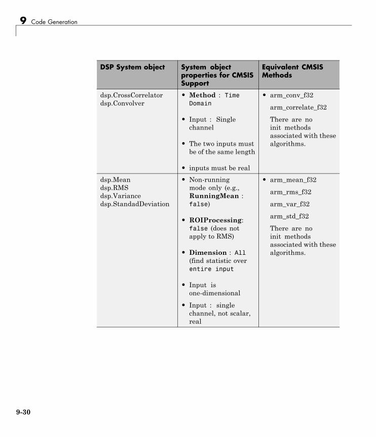
9 Code Generation
DSP System object System objectproperties for CMSISSupport
Equivalent CMSISMethods
dsp.CrossCorrelatordsp.Convolver
• Method : TimeDomain
• Input : Singlechannel
• The two inputs mustbe of the same length
• inputs must be real
• arm_conv_f32
arm_correlate_f32
There are noinit methodsassociated with thesealgorithms.
dsp.Meandsp.RMSdsp.Variancedsp.StandadDeviation
• Non-runningmode only (e.g.,RunningMean :false)
• ROIProcessing:false (does notapply to RMS)
• Dimension : All(find statistic overentire input
• Input isone-dimensional
• Input : singlechannel, not scalar,real
• arm_mean_f32
arm_rms_f32
arm_var_f32
arm_std_f32
There are noinit methodsassociated with thesealgorithms.
9-30
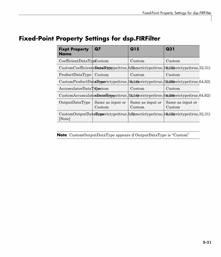
Fixed-Point Property Settings for dsp.FIRFilter
Fixed-Point Property Settings for dsp.FIRFilter
Fixpt PropertyName
Q7 Q15 Q31
CoefficientDataTypeCustom Custom Custom
CustomCoefficientsDataTypenumerictype(true,8,7)numerictype(true,16,15)numerictype(true,32,31)
ProductDataType Custom Custom Custom
CustomProductDataTypenumerictype(true,16,14)numerictype(true,32,30)numerictype(true,64,62)
AccumulatorDataTypeCustom Custom Custom
CustomAccumulatorDataTypenumerictype(true,32,14)numerictype(true,64,30)numerictype(true,64,62)
OutputDataType Same as input orCustom
Same as input orCustom
Same as input orCustom
CustomOutputDataType[Note]
numerictype(true,8,7)numerictype(true,16,15)numerictype(true,32,31)
Note CustomOutputDataType appears if OutputDataType is “Custom”
9-31

9 Code Generation
Fixed-Point Property Settings for Discrete FIR Filter block
Fixed-PointProperty Name
q7 q15 q31
CoefDataTypeStr fixdt(true,8,7) fixdt(true,16,15) fixdt(true,32,31)
ProductDataTypeStrfixdt(true,16,14) fixdt(true,32,30) fixdt(true,64,62)
AccumDataTypeStrfxdt(true,32,14) fxdt(true,64,30) fxdt(true,64,62)
OutputDataType “Inherit: Sameas input” orfxdt(true,8,7)
“Inherit: Sameas input” orfxpt(true,16,15)
“Inherit: Sameas input” orfxdt(true, 32,31)
9-32

CMSIS Conditions for DSP Blocks to Support ARM Cortex-M
CMSIS Conditions for DSP Blocks to Support ARM Cortex-M
In this section...
“General Conditions on All Blocks” on page 9-33
“Specific Block Parameters Used to Support CMSIS ” on page 9-33
General Conditions on All BlocksUnder the following conditions, CMSIS support for DSP blocks is available:
• Input data type is single. (except for Discrete FIR Filter with 'DirectForm' Structure, where both single and fixed-point data types aresupported.)
• Block is in single rate mode.
• Input or output is real. (Support for complex input or output is availablefor FFT and IFFT blocks.)
• Input is single channel.
Note In the Fixed-point mode of the CMSIS DSP (FIR) function, Wrap isused for intermediate MAC operations if accumulator result overflows. At theend, the accumulator is right shifted and saturated to the output data type.For discrete FIR block or system object, there is only one overflow settingfor accumulator and output. So if overflow happens in accumulation, thesimulation result will not match the CMSIS library result.
Specific Block Parameters Used to Support CMSISDSP blocks supporting the ARM-Cortex-M package require a set of conditionsthat would allow code replacement with the CMSIS Library, when generatingC code from a model. The CMSIS library supports these DSP blocks onlywhen you set specific parameters, as indicated in the following table. To usethe CMSIS library with these blocks offering ARM support, you must followthese rules for specifying parameters.
9-33

9 Code Generation
The following table illustrates the rules under which CMSIS supports theseblocks offering ARM support:
DSP Block Block Parameters forCMSIS Support
Equivalent CMSISMethods
Discrete FIR Filter • Filter structure:Direct Form orLattice MA
• Input is real
Input processing:Columns as channels(frame based); andinput has one column
Input : singlechannel
• Initial states : 0
• Coefficientssource: Dialogparameters or Inputport
• The followingsettings are neededto support fixed-pointDiscrete FIR Filterblock, in DirectForm Structureonly:
• RndMeth:'Floor'
• SaturateOnIntegerOverflow:on
• 'Direct Form'Structure:
• arm_fir_f32
• arm_fir_init_f32
• fixed-point inputwith q7 format:
• arm_fir_q7
• arm_fir_init_q7
• fixed-point inputwith q15 format:
• arm_fir_q15
• arm_fir_init_q15
• fixed-point inputwith q31 format:
• arm_fir_q31
• arm_fir_init_q31
• 'Lattice MA'Structure:
• arm_fir_lattice_f32
9-34
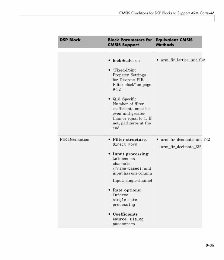
CMSIS Conditions for DSP Blocks to Support ARM Cortex-M
DSP Block Block Parameters forCMSIS Support
Equivalent CMSISMethods
• lockScale: on
• “Fixed-PointProperty Settingsfor Discrete FIRFilter block” on page9-32
• Q15 Specific:Number of filtercoefficients must beeven and greaterthan or equal to 4. Ifnot, pad zeros at theend.
• arm_fir_lattice_init_f32
FIR Decimation • Filter structure:Direct Form
• Input processing:Columns aschannels(frame-based), andinput has one column
Input: single channel
• Rate options:Enforcesingle-rateprocessing
• Coefficientssource: Dialogparameters
• arm_fir_decimate_init_f32
arm_fir_decimate_f32
9-35

9 Code Generation
DSP Block Block Parameters forCMSIS Support
Equivalent CMSISMethods
FIR Interpolation • Input processing: Columns aschannels (framebased), and inputhas one column
Input: single channel
• Rate options:Enforcesingle-rateprocessing
• Coefficientssource: Dialogparameters
• arm_fir_interpolate_init_f32
arm_fir_interpolate_f32
LMS Filter • Specify step sizevia: Dialog (muspecified from thedialog)
• Reset port :None (noreset port)
• Output filterweights : off (noweights output port)
• Adapt port : off (noadapt output port)
• Leakage : 1
• Initial value offilter weights : 0(initial weights arezero)
• arm_lms_init_f32
• arm_lms_f32
If the algorithm isNormalized LMS:
- arm_lms_norm_f32
- arm_lms_norm_init_f32
9-36
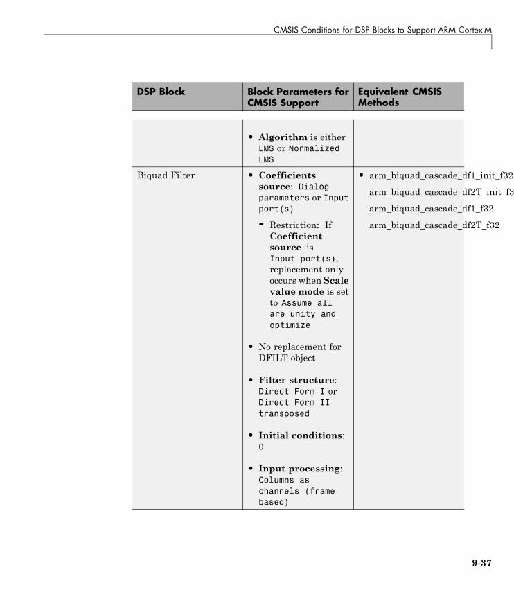
CMSIS Conditions for DSP Blocks to Support ARM Cortex-M
DSP Block Block Parameters forCMSIS Support
Equivalent CMSISMethods
• Algorithm is eitherLMS or NormalizedLMS
Biquad Filter • Coefficientssource: Dialogparameters or Inputport(s)
- Restriction: IfCoefficientsource isInput port(s),replacement onlyoccurs when Scalevalue mode is setto Assume allare unity andoptimize
• No replacement forDFILT object
• Filter structure:Direct Form I orDirect Form IItransposed
• Initial conditions:0
• Input processing:Columns aschannels (framebased)
• arm_biquad_cascade_df1_init_f32
arm_biquad_cascade_df2T_init_f3
arm_biquad_cascade_df1_f32
arm_biquad_cascade_df2T_f32
9-37
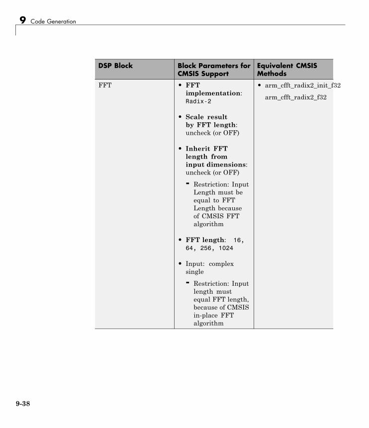
9 Code Generation
DSP Block Block Parameters forCMSIS Support
Equivalent CMSISMethods
FFT • FFTimplementation:Radix-2
• Scale resultby FFT length:uncheck (or OFF)
• Inherit FFTlength frominput dimensions:uncheck (or OFF)
- Restriction: InputLength must beequal to FFTLength becauseof CMSIS FFTalgorithm
• FFT length: 16,64, 256, 1024
• Input: complexsingle
- Restriction: Inputlength mustequal FFT length,because of CMSISin-place FFTalgorithm
• arm_cfft_radix2_init_f32
arm_cfft_radix2_f32
9-38
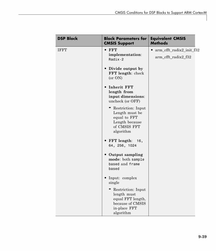
CMSIS Conditions for DSP Blocks to Support ARM Cortex-M
DSP Block Block Parameters forCMSIS Support
Equivalent CMSISMethods
IFFT • FFTimplementation:Radix-2
• Divide output byFFT length: check(or ON)
• Inherit FFTlength frominput dimensions:uncheck (or OFF)
- Restriction: InputLength must beequal to FFTLength becauseof CMSIS FFTalgorithm
• FFT length: 16,64, 256, 1024
• Output samplingmode: both samplebased and framebased
• Input: complexsingle
- Restriction: Inputlength mustequal FFT length,because of CMSISin-place FFTalgorithm
• arm_cfft_radix2_init_f32
arm_cfft_radix2_f32
9-39

9 Code Generation
DSP Block Block Parameters forCMSIS Support
Equivalent CMSISMethods
CorrelationConvolution
• Computationdomain: Time
• Input: Singlechannel
• The two inputs mustbe of the same length
• inputs must be real
• arm_conv_f32
arm_correlate_f32
There are noinit methodsassociated with thesealgorithms.
MeanRMSVarianceStandard deviation
• Non-running modeonly
• ROI Processing:disabled (does notapply to RMS)
• Find statistic overentire input
• Input isone-dimensional
• Input: singlechannel, not scalar,real
• arm_mean_f32
arm_rms_f32
arm_var_f32
arm_std_f32
There are noinit methodsassociated with thesealgorithms.
9-40

Support Packages and Support Package Installer
Support Packages and Support Package Installer
What Is a Support Package?A support package is an add-on that enables you to use a MathWorks® productwith specific third-party hardware and software.
Support packages can include:
• Simulink block libraries
• MATLAB functions, classes, and methods
• Firmware updates for the third-party hardware
• Automatic installation of third-party software
• Examples and tutorials
A support package file has a *.zip extension. This type of file containsMATLAB files, MEX files, and other supporting files required to install thesupport package. Use Support Package Installer to install these supportpackage files.
A support package installation file has a *.mlpkginstall extension. Youcan double click this type of file to start Support Package Installer, whichpreselects a specific support package for installation. You can download thesefiles from MATLAB Central File Exchange and use them to share supportpackages with others.
What Is Support Package Installer?Support Package Installer is a wizard that guides you through the process ofinstalling support packages.
You can use Support Package Installer to:
• Display a list of available, installable, installed, or updatable supportpackages
• Install, update, download, or uninstall a support package.
• Update the firmware on specific third-party hardware.
9-41
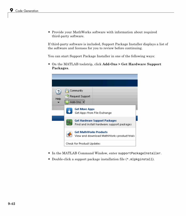
9 Code Generation
• Provide your MathWorks software with information about requiredthird-party software.
If third-party software is included, Support Package Installer displays a list ofthe software and licenses for you to review before continuing.
You can start Support Package Installer in one of the following ways:
• On the MATLAB toolstrip, click Add-Ons > Get Hardware SupportPackages.
• In the MATLAB Command Window, enter supportPackageInstaller.
• Double-click a support package installation file (*.mlpkginstall).
9-42
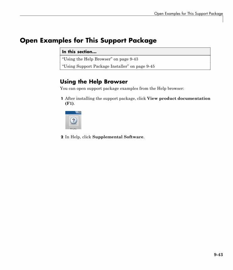
Open Examples for This Support Package
Open Examples for This Support Package
In this section...
“Using the Help Browser” on page 9-43
“Using Support Package Installer” on page 9-45
Using the Help BrowserYou can open support package examples from the Help browser:
1 After installing the support package, click View product documentation(F1).
2 In Help, click Supplemental Software.
9-43

9 Code Generation
3 In Supplemental Software, double-click Examples.
9-44
Open Examples for This Support Package
4 Select the examples for your support package.
Note For other types of examples, open the Help browser and search for yourproduct name followed by “examples”.
Using Support Package InstallerSupport Package Installer (supportPackageInstaller) automaticallydisplays the support package examples when you complete the process ofinstalling and setting up a support package.
On the last screen in Support Package Installer, leave Show supportpackage examples enabled and click Finish.
9-45

9 Code Generation
9-46

Install This Support Package on Other Computers
Install This Support Package on Other ComputersYou can download a support package to one computer, and then install it onother computers. Using this approach, you can:
• Save time when installing support packages on multiple computers.
• Install support packages on computers that are not connected to theInternet.
Before starting, select a computer to use for downloading. This computer musthave the same base product license and platform as the computers upon whichyou are installing the support package. For example, suppose you want toinstall a Simulink support package on a group of computers that are running64-bit Windows. To do so, you must first download the support package usinga computer that has a Simulink license and is running 64-bit Windows.
Download the support package to one computer:
1 In the MATLAB Command Window, enter supportPackageInstaller.
2 In Support Package Installer, on the Select an action screen, chooseDownload from Internet. Click Next.
3 On the following screen, select the support package to download.
Verify the path of the Download folder. For example,C:\MATLAB\SupportPackages\R2013b\downloads.
4 Follow the instructions provided by Support Package Installer to completethe download process.
This action creates a subfolder within the Download folder that containsthe files required for each support package.
5 Make the new folder available to for installation on other computers. Forexample, you can share the folder on the network, or copy the folder toportable media, such as a USB flash drive.
9-47
9 Code Generation
Note Some support packages require you to install third-party software.If so, also make the third-party software available for installation on theother computers.
Install the support package on the other computers:
1 Run Support Package Installer on the other computer or computers.
2 On the Install or update support package screen, select the Folderoption.
3 Click Browse to specify the location of the support package folder on thenetwork or portable media.
4 Follow the instructions provided by Support Package Installer to completethe installation process.
9-48
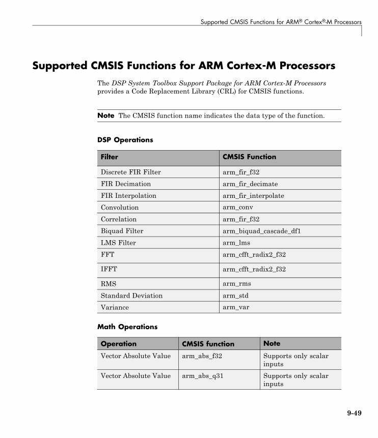
Supported CMSIS Functions for ARM® Cortex®-M Processors
Supported CMSIS Functions for ARM Cortex-M ProcessorsThe DSP System Toolbox Support Package for ARM Cortex-M Processorsprovides a Code Replacement Library (CRL) for CMSIS functions.
Note The CMSIS function name indicates the data type of the function.
DSP Operations
Filter CMSIS Function
Discrete FIR Filter arm_fir_f32
FIR Decimation arm_fir_decimate
FIR Interpolation arm_fir_interpolate
Convolution arm_conv
Correlation arm_fir_f32
Biquad Filter arm_biquad_cascade_df1
LMS Filter arm_lms
FFT arm_cfft_radix2_f32
IFFT arm_cfft_radix2_f32
RMS arm_rms
Standard Deviation arm_std
Variance arm_var
Math Operations
Operation CMSIS function Note
Vector Absolute Value arm_abs_f32 Supports only scalarinputs
Vector Absolute Value arm_abs_q31 Supports only scalarinputs
9-49
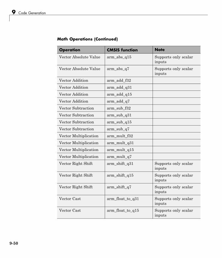
9 Code Generation
Math Operations (Continued)
Operation CMSIS function Note
Vector Absolute Value arm_abs_q15 Supports only scalarinputs
Vector Absolute Value arm_abs_q7 Supports only scalarinputs
Vector Addition arm_add_f32
Vector Addition arm_add_q31
Vector Addition arm_add_q15
Vector Addition arm_add_q7
Vector Subtraction arm_sub_f32
Vector Subtraction arm_sub_q31
Vector Subtraction arm_sub_q15
Vector Subtraction arm_sub_q7
Vector Multiplication arm_mult_f32
Vector Multiplication arm_mult_q31
Vector Multiplication arm_mult_q15
Vector Multiplication arm_mult_q7
Vector Right Shift arm_shift_q31 Supports only scalarinputs
Vector Right Shift arm_shift_q15 Supports only scalarinputs
Vector Right Shift arm_shift_q7 Supports only scalarinputs
Vector Cast arm_float_to_q31 Supports only scalarinputs
Vector Cast arm_float_to_q15 Supports only scalarinputs
9-50

Supported CMSIS Functions for ARM® Cortex®-M Processors
Math Operations (Continued)
Operation CMSIS function Note
Vector Cast arm_float_to_q7 Supports only scalarinputs
Vector Cast arm_q31_to_float Supports only scalarinputs
Vector Cast arm_q31_to_q15 Supports only scalarinputs
Vector Cast arm_q31_to_q7 Supports only scalarinputs
Vector Cast arm_q15_to_float Supports only scalarinputs
Vector Cast arm_q15_to_q31 Supports only scalarinputs
Vector Cast arm_q15_to_q7 Supports only scalarinputs
Vector Cast arm_q7_to_float Supports only scalarinputs
Vector Cast arm_q7_to_q31 Supports only scalarinputs
Vector Cast arm_q7_to_q15 Supports only scalarinputs
Vector Cast arm_shift_q31 Supports only scalarinputs
Vector Cast arm_shift_q15 Supports only scalarinputs
Vector Cast arm_shift_q7 Supports only scalarinputs
Square root arm_sqrt_f32
Square root arm_sqrt_q31
Square root arm_sqrt_q15
9-51

9 Code Generation
Math Operations (Continued)
Operation CMSIS function Note
sin arm_sin_f32
cosine arm_cos_f32
Complex Conjugate arm_cmplx_conj_f32
Complex Conjugate arm_cmplx_conj_q31
Complex Conjugate arm_cmplx_conj_q15
Complex-by-ComplexMultiplication
arm_cmplx_mult_cmplx_f32
Complex-by-ComplexMultiplication
arm_cmplx_mult_cmplx_q31
Complex-by-ComplexMultiplication
arm_cmplx_mult_cmplx_q15
Complex-by-RealMultiplication
arm_cmplx_mult_real_f32
Complex-by-RealMultiplication
arm_cmplx_mult_real_q31
Complex-by-RealMultiplication
arm_cmplx_mult_real_q15
9-52

10
Define New System Objects
• “Define Basic System Objects” on page 10-3
• “Change Number of Step Inputs or Outputs” on page 10-5
• “Specify System Block Input and Output Names” on page 10-8
• “Validate Property and Input Values” on page 10-10
• “Initialize Properties and Setup One-Time Calculations” on page 10-13
• “Set Property Values at Construction Time” on page 10-16
• “Reset Algorithm State” on page 10-19
• “Define Property Attributes” on page 10-21
• “Hide Inactive Properties” on page 10-25
• “Limit Property Values to Finite String Set” on page 10-27
• “Process Tuned Properties” on page 10-30
• “Release System Object Resources” on page 10-32
• “Define Composite System Objects” on page 10-34
• “Define Finite Source Objects” on page 10-38
• “Save System Object” on page 10-40
• “Load System Object” on page 10-43
• “Clone System Object” on page 10-46
• “Define System Object Information” on page 10-47
• “Define System Block Icon” on page 10-49
• “Add Header to System Block Dialog” on page 10-51
• “Add Property Groups to System Object and Block Dialog” on page 10-53

10 Define New System Objects
• “Set Output Size” on page 10-57
• “Set Output Data Type” on page 10-60
• “Set Output Complexity” on page 10-63
• “Specify Whether Output Is Fixed- or Variable-Size” on page 10-66
• “Specify Discrete State Output Specification” on page 10-69
• “Use Update and Output for Nondirect Feedthrough” on page 10-72
• “Methods Timing” on page 10-75
• “System Object Input Arguments and ~ in Code Examples” on page 10-78
• “What Are Mixin Classes?” on page 10-79
• “Best Practices for Defining System Objects” on page 10-80
10-2

Define Basic System Objects
Define Basic System ObjectsThis example shows how to create a basic System object that increments anumber by one.
The class definition file contains the minimum elements required to definea System object.
Create the Class Definition File
1 Create a MATLAB file named AddOne.m to contain the definition of yourSystem object.
edit AddOne.m
2 Subclass your object from matlab.System. Insert this line as the first lineof your file.
classdef AddOne < matlab.System
3 Add the stepImpl method, which contains the algorithm that runs whenusers call the step method on your object. You always set the stepImplmethod access to protected because it is an internal method that usersdo not directly call or run.
All methods, except static methods, expect the System object handle as thefirst input argument. You can use any name for your System object handle.
In this example, instead of passing in the object handle, ~ is used to indicatethat the object handle is not used in the function. Using ~ instead of anobject handle prevents warnings about unused variables from occurring.
By default, the number of inputs and outputs are both one. Tochange the number of inputs or outputs, use the getNumInputsImpl orgetNumOutputsImpl method, respectively.
methods (Access=protected)function y = stepImpl(~, x)
y = x + 1;end
end
10-3
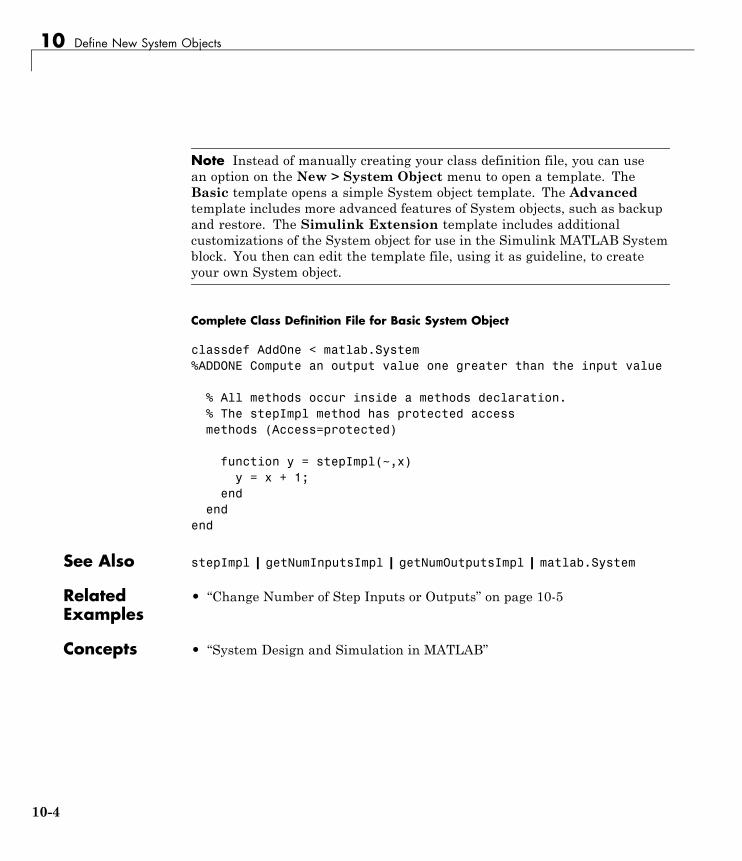
10 Define New System Objects
Note Instead of manually creating your class definition file, you can usean option on the New > System Object menu to open a template. TheBasic template opens a simple System object template. The Advancedtemplate includes more advanced features of System objects, such as backupand restore. The Simulink Extension template includes additionalcustomizations of the System object for use in the Simulink MATLAB Systemblock. You then can edit the template file, using it as guideline, to createyour own System object.
Complete Class Definition File for Basic System Object
classdef AddOne < matlab.System%ADDONE Compute an output value one greater than the input value
% All methods occur inside a methods declaration.% The stepImpl method has protected accessmethods (Access=protected)
function y = stepImpl(~,x)y = x + 1;
endend
end
See Also stepImpl | getNumInputsImpl | getNumOutputsImpl | matlab.System
RelatedExamples
• “Change Number of Step Inputs or Outputs” on page 10-5
Concepts • “System Design and Simulation in MATLAB”
10-4
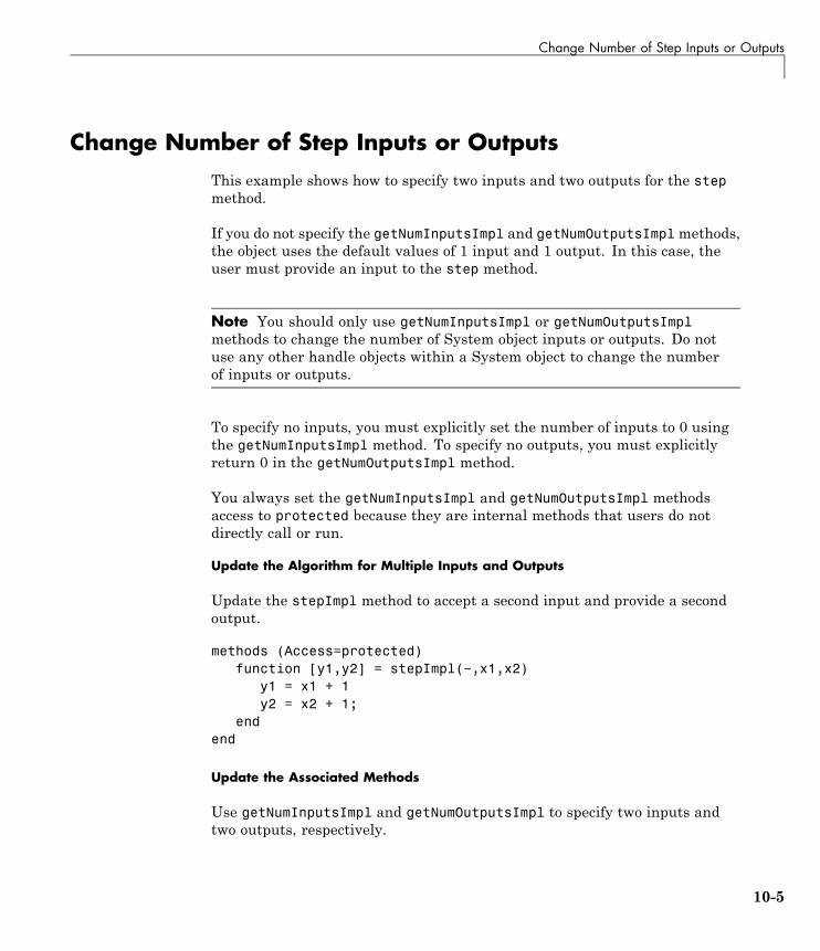
Change Number of Step Inputs or Outputs
Change Number of Step Inputs or OutputsThis example shows how to specify two inputs and two outputs for the stepmethod.
If you do not specify the getNumInputsImpl and getNumOutputsImplmethods,the object uses the default values of 1 input and 1 output. In this case, theuser must provide an input to the step method.
Note You should only use getNumInputsImpl or getNumOutputsImplmethods to change the number of System object inputs or outputs. Do notuse any other handle objects within a System object to change the numberof inputs or outputs.
To specify no inputs, you must explicitly set the number of inputs to 0 usingthe getNumInputsImpl method. To specify no outputs, you must explicitlyreturn 0 in the getNumOutputsImpl method.
You always set the getNumInputsImpl and getNumOutputsImpl methodsaccess to protected because they are internal methods that users do notdirectly call or run.
Update the Algorithm for Multiple Inputs and Outputs
Update the stepImpl method to accept a second input and provide a secondoutput.
methods (Access=protected)function [y1,y2] = stepImpl(~,x1,x2)
y1 = x1 + 1y2 = x2 + 1;
endend
Update the Associated Methods
Use getNumInputsImpl and getNumOutputsImpl to specify two inputs andtwo outputs, respectively.
10-5
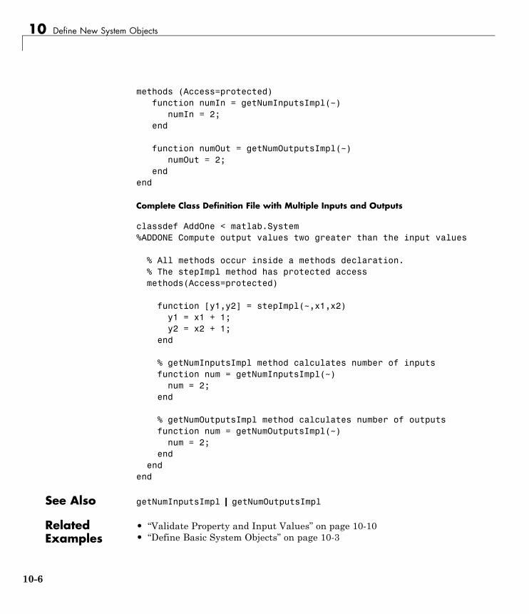
10 Define New System Objects
methods (Access=protected)function numIn = getNumInputsImpl(~)
numIn = 2;end
function numOut = getNumOutputsImpl(~)numOut = 2;
endend
Complete Class Definition File with Multiple Inputs and Outputs
classdef AddOne < matlab.System%ADDONE Compute output values two greater than the input values
% All methods occur inside a methods declaration.% The stepImpl method has protected accessmethods(Access=protected)
function [y1,y2] = stepImpl(~,x1,x2)y1 = x1 + 1;y2 = x2 + 1;
end
% getNumInputsImpl method calculates number of inputsfunction num = getNumInputsImpl(~)
num = 2;end
% getNumOutputsImpl method calculates number of outputsfunction num = getNumOutputsImpl(~)
num = 2;end
endend
See Also getNumInputsImpl | getNumOutputsImpl
RelatedExamples
• “Validate Property and Input Values” on page 10-10• “Define Basic System Objects” on page 10-3
10-6

Change Number of Step Inputs or Outputs
Concepts • “System Object Input Arguments and ~ in Code Examples” on page 10-78
10-7
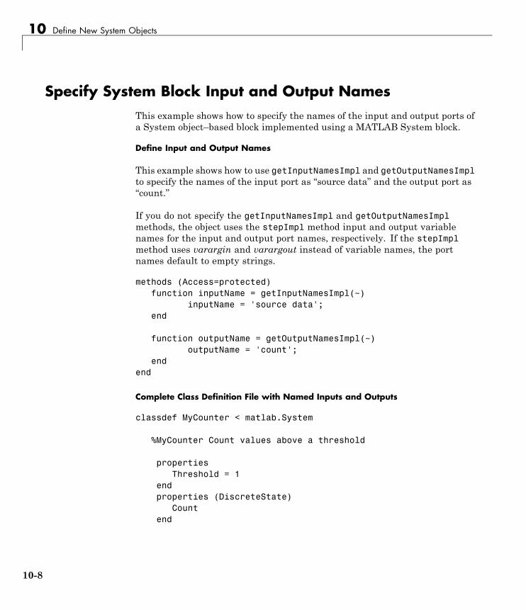
10 Define New System Objects
Specify System Block Input and Output NamesThis example shows how to specify the names of the input and output ports ofa System object–based block implemented using a MATLAB System block.
Define Input and Output Names
This example shows how to use getInputNamesImpl and getOutputNamesImplto specify the names of the input port as “source data” and the output port as“count.”
If you do not specify the getInputNamesImpl and getOutputNamesImplmethods, the object uses the stepImpl method input and output variablenames for the input and output port names, respectively. If the stepImplmethod uses varargin and varargout instead of variable names, the portnames default to empty strings.
methods (Access=protected)function inputName = getInputNamesImpl(~)
inputName = 'source data';end
function outputName = getOutputNamesImpl(~)outputName = 'count';
endend
Complete Class Definition File with Named Inputs and Outputs
classdef MyCounter < matlab.System
%MyCounter Count values above a threshold
propertiesThreshold = 1
endproperties (DiscreteState)
Countend
10-8
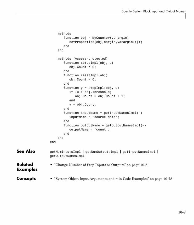
Specify System Block Input and Output Names
methodsfunction obj = MyCounter(varargin)
setProperties(obj,nargin,varargin{:});end
end
methods (Access=protected)function setupImpl(obj, u)
obj.Count = 0;endfunction resetImpl(obj)
obj.Count = 0;endfunction y = stepImpl(obj, u)
if (u > obj.Threshold)obj.Count = obj.Count + 1;
endy = obj.Count;
endfunction inputName = getInputNamesImpl(~)
inputName = 'source data';endfunction outputName = getOutputNamesImpl(~)
outputName = 'count';end
endend
See Also getNumInputsImpl | getNumOutputsImpl | getInputNamesImpl |getOutputNamesImpl
RelatedExamples
• “Change Number of Step Inputs or Outputs” on page 10-5
Concepts • “System Object Input Arguments and ~ in Code Examples” on page 10-78
10-9
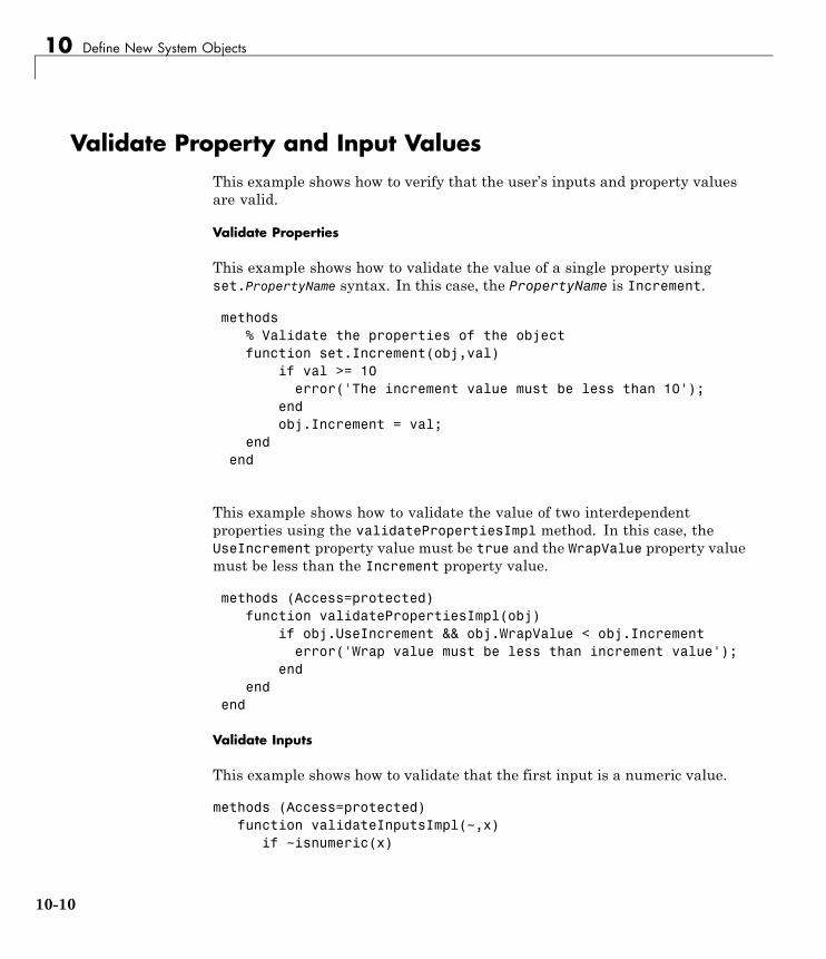
10 Define New System Objects
Validate Property and Input ValuesThis example shows how to verify that the user’s inputs and property valuesare valid.
Validate Properties
This example shows how to validate the value of a single property usingset.PropertyName syntax. In this case, the PropertyName is Increment.
methods% Validate the properties of the objectfunction set.Increment(obj,val)
if val >= 10error('The increment value must be less than 10');
endobj.Increment = val;
endend
This example shows how to validate the value of two interdependentproperties using the validatePropertiesImpl method. In this case, theUseIncrement property value must be true and the WrapValue property valuemust be less than the Increment property value.
methods (Access=protected)function validatePropertiesImpl(obj)
if obj.UseIncrement && obj.WrapValue < obj.Incrementerror('Wrap value must be less than increment value');
endend
end
Validate Inputs
This example shows how to validate that the first input is a numeric value.
methods (Access=protected)function validateInputsImpl(~,x)
if ~isnumeric(x)
10-10
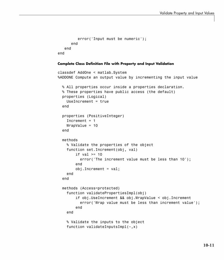
Validate Property and Input Values
error('Input must be numeric');end
endend
Complete Class Definition File with Property and Input Validation
classdef AddOne < matlab.System%ADDONE Compute an output value by incrementing the input value
% All properties occur inside a properties declaration.% These properties have public access (the default)properties (Logical)
UseIncrement = trueend
properties (PositiveInteger)Increment = 1WrapValue = 10
end
methods% Validate the properties of the objectfunction set.Increment(obj, val)
if val >= 10error('The increment value must be less than 10');
endobj.Increment = val;
endend
methods (Access=protected)function validatePropertiesImpl(obj)
if obj.UseIncrement && obj.WrapValue < obj.Incrementerror('Wrap value must be less than increment value');
endend
% Validate the inputs to the objectfunction validateInputsImpl(~,x)
10-11
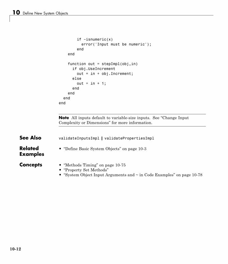
10 Define New System Objects
if ~isnumeric(x)error('Input must be numeric');
endend
function out = stepImpl(obj,in)if obj.UseIncrement
out = in + obj.Increment;else
out = in + 1;end
endend
end
Note All inputs default to variable-size inputs. See “Change InputComplexity or Dimensions” for more information.
See Also validateInputsImpl | validatePropertiesImpl
RelatedExamples
• “Define Basic System Objects” on page 10-3
Concepts • “Methods Timing” on page 10-75• “Property Set Methods”• “System Object Input Arguments and ~ in Code Examples” on page 10-78
10-12
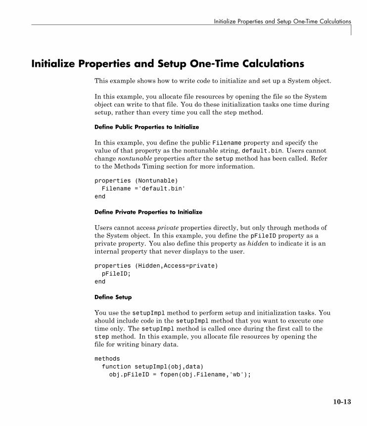
Initialize Properties and Setup One-Time Calculations
Initialize Properties and Setup One-Time CalculationsThis example shows how to write code to initialize and set up a System object.
In this example, you allocate file resources by opening the file so the Systemobject can write to that file. You do these initialization tasks one time duringsetup, rather than every time you call the step method.
Define Public Properties to Initialize
In this example, you define the public Filename property and specify thevalue of that property as the nontunable string, default.bin. Users cannotchange nontunable properties after the setup method has been called. Referto the Methods Timing section for more information.
properties (Nontunable)Filename ='default.bin'
end
Define Private Properties to Initialize
Users cannot access private properties directly, but only through methods ofthe System object. In this example, you define the pFileID property as aprivate property. You also define this property as hidden to indicate it is aninternal property that never displays to the user.
properties (Hidden,Access=private)pFileID;
end
Define Setup
You use the setupImpl method to perform setup and initialization tasks. Youshould include code in the setupImpl method that you want to execute onetime only. The setupImpl method is called once during the first call to thestep method. In this example, you allocate file resources by opening thefile for writing binary data.
methodsfunction setupImpl(obj,data)
obj.pFileID = fopen(obj.Filename,'wb');
10-13

10 Define New System Objects
if obj.pFileID < 0error('Opening the file failed');
endend
end
Although not part of setup, you should close files when your code is done usingthem. You use the releaseImpl method to release resources.
Complete Class Definition File with Initialization and Setup
classdef MyFile < matlab.System%MyFile write numbers to a file
% These properties are nontunable. They cannot be changed% after the setup or step method has been called.properties (Nontunable)
Filename ='default.bin' % the name of the file to createend
% These properties are private. Customers can only access% these properties through methods on this objectproperties (Hidden,Access=private)
pFileID; % The identifier of the file to openend
methods (Access=protected)% In setup allocate any resources, which in this case% means opening the file.function setupImpl(obj,data)
obj.pFileID = fopen(obj.Filename,'wb');if obj.pFileID < 0
error('Opening the file failed');end
end
% This System object writes the input to the file.function stepImpl(obj,data)
fwrite(obj.pFileID,data);end
10-14
Initialize Properties and Setup One-Time Calculations
% Use release to close the file to prevent the% file handle from being left open.function releaseImpl(obj)
fclose(obj.pFileID);end
% You indicate that no outputs are provided by returning% zero from getNumOutputsImplfunction numOutputs = getNumOutputsImpl(~)
numOutputs = 0;end
endend
See Also setupImpl | releaseImpl | stepImpl
RelatedExamples
• “Release System Object Resources” on page 10-32• “Define Property Attributes” on page 10-21
Concepts • “Methods Timing” on page 10-75
10-15
10 Define New System Objects
Set Property Values at Construction TimeThis example shows how to define a System object constructor and allow it toaccept name-value property pairs as input.
Set Properties to Use Name-Value Pair Input
Define the System object constructor, which is a method that has the samename as the class (MyFile in this example). Within that method, you usethe setProperties method to make all public properties available for inputwhen the user constructs the object. nargin is a MATLAB function thatdetermines the number of input arguments. varargin indicates all of theobject’s public properties.
methodsfunction obj = MyFile(varargin)
setProperties(obj,nargin,varargin{:});end
end
Complete Class Definition File with Constructor Setup
classdef MyFile < matlab.System%MyFile write numbers to a file
% These properties are nontunable. They cannot be changed% after the setup or step method has been called.properties (Nontunable)
Filename ='default.bin' % the name of the file to createAccess = 'wb' % The file access string (write, binary)
end
% These properties are private. Customers can only access% these properties through methods on this objectproperties (Hidden,Access=private)
pFileID; % The identifier of the file to openend
methods% You call setProperties in the constructor to let
10-16

Set Property Values at Construction Time
% a user specify public properties of object as% name-value pairs.function obj = MyFile(varargin)
setProperties(obj,nargin,varargin{:});end
end
methods (Access=protected)% In setup allocate any resources, which in this case is% opening the file.function setupImpl(obj, ~)
obj.pFileID = fopen(obj.Filename,obj.Access);if obj.pFileID < 0
error('Opening the file failed');end
end
% This System object writes the input to the file.function stepImpl(obj, data)
fwrite(obj.pFileID,data);end
% Use release to close the file to prevent the% file handle from being left open.function releaseImpl(obj)
fclose(obj.pFileID);end% You indicate that no outputs are provided by returning% zero from getNumOutputsImplfunction numOutputs = getNumOutputsImpl(~)
numOutputs = 0;end
endend
See Also nargin | setProperties
10-17

10 Define New System Objects
RelatedExamples
• “Define Property Attributes” on page 10-21• “Release System Object Resources” on page 10-32
10-18
Reset Algorithm State
Reset Algorithm StateThis example shows how to reset an object state.
Reset Counter to Zero
pCount is an internal counter property of the System object obj. The usercalls the reset method, which calls the resetImpl method. In this example, pCount resets to 0.
Note When resetting an object’s state, make sure you reset the size,complexity, and data type correctly.
methods (Access=protected)function resetImpl(obj)
obj.pCount = 0;end
end
Complete Class Definition File with State Reset
classdef Counter < matlab.System%Counter System object that increments a counter
properties(Access=private)pCount
end
methods (Access=protected)% In step, increment the counter and return% its value as an outputfunction c = stepImpl(obj)
obj.pCount = obj.pCount + 1;c = obj.pCount;
end
% Reset the counter to zero.function resetImpl(obj)
10-19
10 Define New System Objects
obj.pCount = 0;end
% The step method takes no inputsfunction numIn = getNumInputsImpl(~)
numIn = 0;end
endendend
See “Methods Timing” on page 10-75 for more information.
See Also resetImpl
Concepts • “Methods Timing” on page 10-75
10-20

Define Property Attributes
Define Property AttributesThis example shows how to specify property attributes.
Property attributes, which add details to a property, provide a layer of controlto your properties. In addition to the MATLAB property attributes, Systemobjects can use these three additional attributes—nontunable, logical,and positiveInteger. To specify multiple attributes, separate them withcommas.
Specify Property as Nontunable
Use the nontunable attribute for a property when the algorithm depends onthe value being constant once data processing starts. Defining a property asnontunable may improve the efficiency of your algorithm by removing theneed to check for or react to values that change. For code generation, defininga property as nontunable allows the memory associated with that propertyto be optimized. You should define all properties that affect the number ofinput or output ports as nontunable.
System object users cannot change nontunable properties after the setup orstep method has been called. In this example, you define the InitialValueproperty, and set its value to 0.
properties (Nontunable)InitialValue = 0;
end
Specify Property as Logical
Logical properties have the value, true or false. System object users canenter 1 or 0 or any value that can be converted to a logical. The value,however, displays as true or false. You can use sparse logical values, butthey must be scalar values. In this example, the Increment property indicateswhether to increase the counter. By default, Increment is tunable property.The following restrictions apply to a property with the Logical attribute,
• Cannot also be Dependent or PositiveInteger
• Default value must be true or false. You cannot use 1 or 0 as a defaultvalue.
10-21
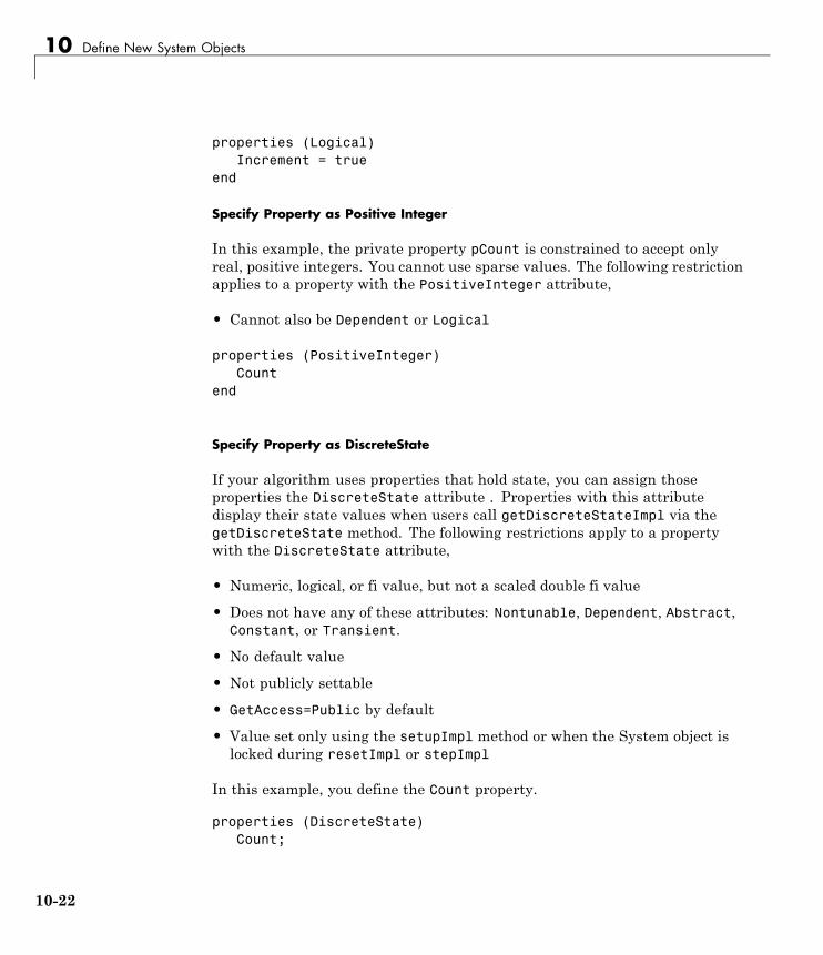
10 Define New System Objects
properties (Logical)Increment = true
end
Specify Property as Positive Integer
In this example, the private property pCount is constrained to accept onlyreal, positive integers. You cannot use sparse values. The following restrictionapplies to a property with the PositiveInteger attribute,
• Cannot also be Dependent or Logical
properties (PositiveInteger)Count
end
Specify Property as DiscreteState
If your algorithm uses properties that hold state, you can assign thoseproperties the DiscreteState attribute . Properties with this attributedisplay their state values when users call getDiscreteStateImpl via thegetDiscreteState method. The following restrictions apply to a propertywith the DiscreteState attribute,
• Numeric, logical, or fi value, but not a scaled double fi value
• Does not have any of these attributes: Nontunable, Dependent, Abstract,Constant, or Transient.
• No default value
• Not publicly settable
• GetAccess=Public by default
• Value set only using the setupImpl method or when the System object islocked during resetImpl or stepImpl
In this example, you define the Count property.
properties (DiscreteState)Count;
10-22
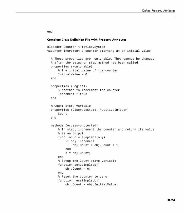
Define Property Attributes
end
Complete Class Definition File with Property Attributes
classdef Counter < matlab.System%Counter Increment a counter starting at an initial value
% These properties are nontunable. They cannot be changed% after the setup or step method has been called.properties (Nontunable)
% The inital value of the counterInitialValue = 0
end
properties (Logical)% Whether to increment the counterIncrement = true
end
% Count state variableproperties (DiscreteState, PositiveInteger)
Countend
methods (Access=protected)% In step, increment the counter and return its value% as an outputfunction c = stepImpl(obj)
if obj.Incrementobj.Count = obj.Count + 1;
endc = obj.Count;
end% Setup the Count state variablefunction setupImpl(obj)
obj.Count = 0;end% Reset the counter to zero.function resetImpl(obj)
obj.Count = obj.InitialValue;
10-23

10 Define New System Objects
end% The step method takes no inputsfunction numIn = getNumInputsImpl(~)
numIn = 0;end
endend
Concepts • “Class Attributes”• “Property Attributes”• “What You Cannot Change While Your System Is Running”• “Methods Timing” on page 10-75
10-24
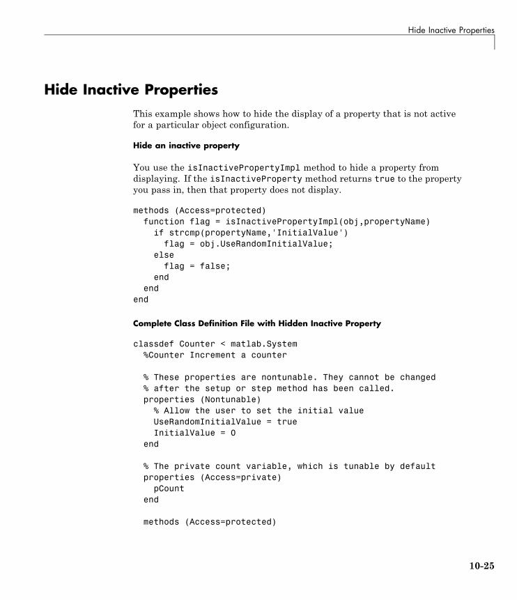
Hide Inactive Properties
Hide Inactive PropertiesThis example shows how to hide the display of a property that is not activefor a particular object configuration.
Hide an inactive property
You use the isInactivePropertyImpl method to hide a property fromdisplaying. If the isInactiveProperty method returns true to the propertyyou pass in, then that property does not display.
methods (Access=protected)function flag = isInactivePropertyImpl(obj,propertyName)
if strcmp(propertyName,'InitialValue')flag = obj.UseRandomInitialValue;
elseflag = false;
endend
end
Complete Class Definition File with Hidden Inactive Property
classdef Counter < matlab.System%Counter Increment a counter
% These properties are nontunable. They cannot be changed% after the setup or step method has been called.properties (Nontunable)
% Allow the user to set the initial valueUseRandomInitialValue = trueInitialValue = 0
end
% The private count variable, which is tunable by defaultproperties (Access=private)
pCountend
methods (Access=protected)
10-25
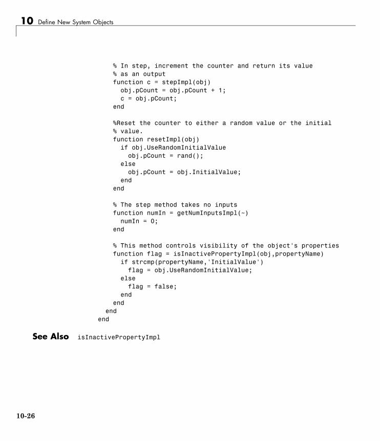
10 Define New System Objects
% In step, increment the counter and return its value% as an outputfunction c = stepImpl(obj)
obj.pCount = obj.pCount + 1;c = obj.pCount;
end
%Reset the counter to either a random value or the initial% value.function resetImpl(obj)
if obj.UseRandomInitialValueobj.pCount = rand();
elseobj.pCount = obj.InitialValue;
endend
% The step method takes no inputsfunction numIn = getNumInputsImpl(~)
numIn = 0;end
% This method controls visibility of the object's propertiesfunction flag = isInactivePropertyImpl(obj,propertyName)
if strcmp(propertyName,'InitialValue')flag = obj.UseRandomInitialValue;
elseflag = false;
endend
endend
See Also isInactivePropertyImpl
10-26
Limit Property Values to Finite String Set
Limit Property Values to Finite String SetThis example shows how to limit a property to accept only a finite set ofstring values.
Specify a Set of Valid String Values
String sets use two related properties. You first specify the user-visibleproperty name and default string value. Then, you specify the associatedhidden property by appending “Set” to the property name. You must usea capital “S” in “Set.”
In the “Set” property, you specify the valid string values as a cell array of thematlab.system.Stringset class. This example uses Color and ColorSetas the associated properties.
propertiesColor = 'blue'
end
properties (Hidden,Transient)ColorSet = matlab.system.StringSet({'red','blue','green'});
end
Complete Class Definition File with String Set
classdef Whiteboard < matlab.System%Whiteboard Draw lines on a figure window%% This System object illustrates the use of StringSets
propertiesColor = 'blue'
end
properties (Hidden,Transient)% Let them choose a colorColorSet = matlab.system.StringSet({'red','blue','green'});
end
10-27
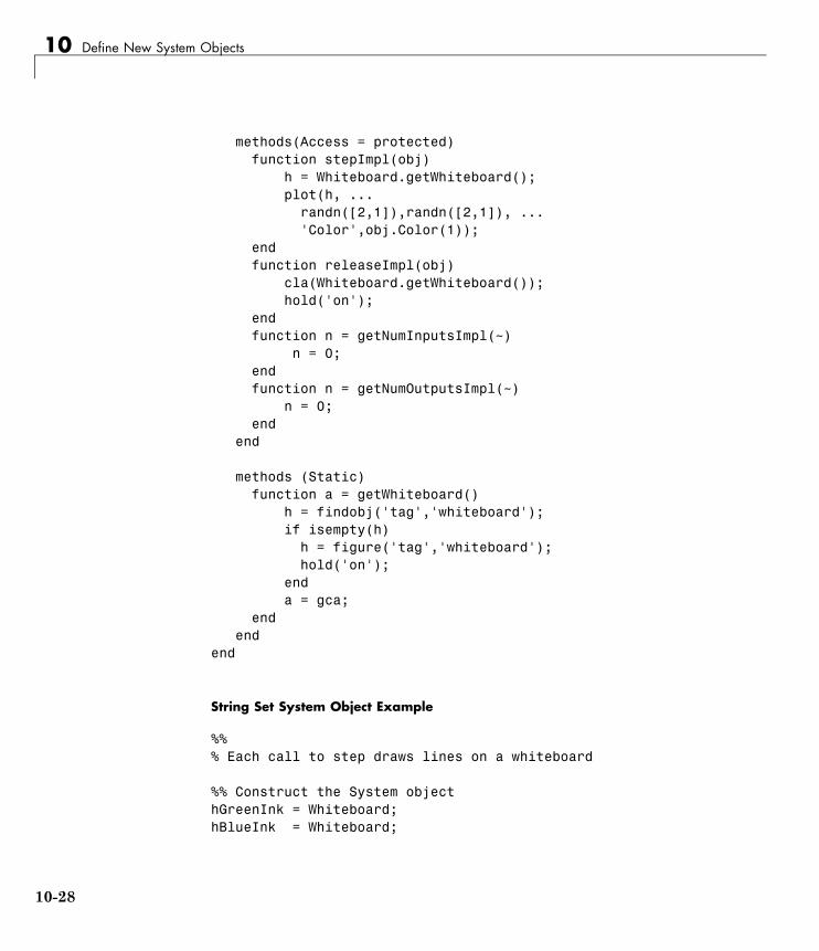
10 Define New System Objects
methods(Access = protected)function stepImpl(obj)
h = Whiteboard.getWhiteboard();plot(h, ...
randn([2,1]),randn([2,1]), ...'Color',obj.Color(1));
endfunction releaseImpl(obj)
cla(Whiteboard.getWhiteboard());hold('on');
endfunction n = getNumInputsImpl(~)
n = 0;endfunction n = getNumOutputsImpl(~)
n = 0;end
end
methods (Static)function a = getWhiteboard()
h = findobj('tag','whiteboard');if isempty(h)
h = figure('tag','whiteboard');hold('on');
enda = gca;
endend
end
String Set System Object Example
%%% Each call to step draws lines on a whiteboard
%% Construct the System objecthGreenInk = Whiteboard;hBlueInk = Whiteboard;
10-28
Limit Property Values to Finite String Set
% Change the color% Note: Press tab after typing the first single quote to% display all enumerated values.hGreenInk.Color = 'green';hBlueInk.Color = 'blue';
% Take a few stepsfor i=1:3
hGreenInk.step();hBlueInk.step();
end
%% Clear the whiteboardhBlueInk.release();
%% Display System object used in this exampletype('Whiteboard.m');
See Also matlab.system.StringSet
10-29

10 Define New System Objects
Process Tuned PropertiesThis example shows how to specify the action to take when a tunable propertyvalue changes during simulation.
The processTunedPropertiesImpl method is useful for managing actions toprevent duplication. In many cases, changing one of multiple interdependentproperties causes an action. With the processTunedPropertiesImpl method,you can control when that action is taken so it is not repeated unnecessarily.
Control When a Lookup Table Is Generated
This example of processTunedPropertiesImpl causes the pLookupTable tobe regenerated when either the NumNotes or MiddleC property changes.
methods (Access = protected)function processTunedPropertiesImpl(obj)
obj.pLookupTable = obj.MiddleC * ...(1+log(1:obj.NumNotes)/log(12));
endend
Complete Class Definition File with Tuned Property Processing
classdef TuningFork < matlab.System%TuningFork Illustrate the processing of tuned parameters%
propertiesMiddleC = 440NumNotes = 12
end
properties (Access=private)pLookupTable
end
methods(Access=protected)function resetImpl(obj)
obj.MiddleC = 440;
10-30

Process Tuned Properties
obj.pLookupTable = obj.MiddleC * ...(1+log(1:obj.NumNotes)/log(12));
end
function hz = stepImpl(obj,noteShift)% A noteShift value of 1 corresponds to obj.MiddleChz = obj.pLookupTable(noteShift);
end
function processTunedPropertiesImpl(obj)% Generate a lookup table of note frequenciesobj.pLookupTable = obj.MiddleC * ...
(1+log(1:obj.NumNotes)/log(12));end
endend
See Also processTunedPropertiesImpl
10-31

10 Define New System Objects
Release System Object ResourcesThis example shows how to release resources allocated and used by theSystem object. These resources include allocated memory, files used forreading or writing, etc.
Release Memory by Clearing the Object
This method allows you to clear the axes on the Whiteboard figure windowwhile keeping the figure open.
methodsfunction releaseImpl(obj)
cla(Whiteboard.getWhiteboard());hold('on');
endend
Complete Class Definition File with Released Resources
classdef Whiteboard < matlab.System%Whiteboard Draw lines on a figure window%% This System object shows the use of StringSets%
propertiesColor = 'blue'
end
properties (Hidden)% Let user choose a colorColorSet = matlab.system.StringSet({'red','blue','green'});
end
methods(Access=protected)function stepImpl(obj)
h = Whiteboard.getWhiteboard();plot(h, ...
randn([2,1]), randn([2,1]), ...'Color',obj.Color(1));
10-32

Release System Object Resources
end
function releaseImpl(obj)cla(Whiteboard.getWhiteboard());hold('on');
end
function n = getNumInputsImpl(~)n = 0;
endfunction n = getNumOutputsImpl(~)
n = 0;end
end
methods (Static)function a = getWhiteboard()
h = findobj('tag','whiteboard');if isempty(h)
h = figure('tag','whiteboard');hold('on');
enda = gca;
endend
end
See Also releaseImpl
RelatedExamples
• “Initialize Properties and Setup One-Time Calculations” on page 10-13
10-33
10 Define New System Objects
Define Composite System ObjectsThis example shows how to define System objects that include other Systemobjects.
This example defines a filter System object from an FIR System object andan IIR System object.
Store System Objects in Properties
To define a System object from other System objects, store those objects inyour class definition file as properties. In this example, FIR and IIR areseparate System objects defined in their own class-definition files. You usethose two objects to calculate the pFir and pIir property values.
properties (Nontunable, Access = private)pFir % store the FIR filterpIir % store the IIR filter
end
methodsfunction obj = Filter(varargin)
setProperties(obj, nargin, varargin{:});obj.pFir = FIR(obj.zero);obj.pIir = IIR(obj.pole);
endend
Complete Class Definition File of Composite System Object
classdef Filter < matlab.System% Filter System object with a single pole and a single zero%% This System object illustrates composition by% composing an instance of itself.%
properties (Nontunable)zero = 0.01pole = 0.5
10-34
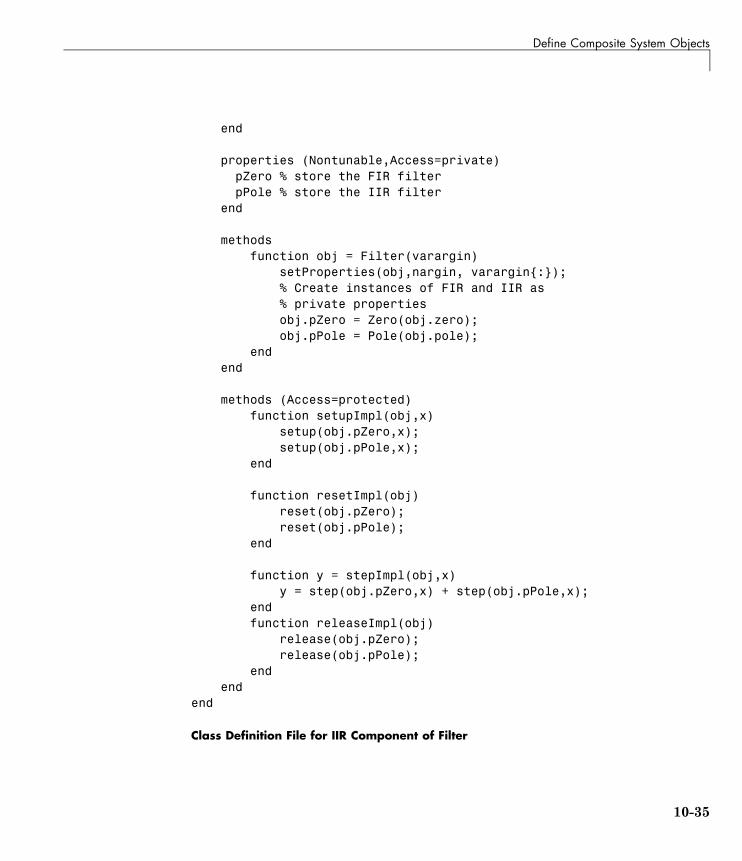
Define Composite System Objects
end
properties (Nontunable,Access=private)pZero % store the FIR filterpPole % store the IIR filter
end
methodsfunction obj = Filter(varargin)
setProperties(obj,nargin, varargin{:});% Create instances of FIR and IIR as% private propertiesobj.pZero = Zero(obj.zero);obj.pPole = Pole(obj.pole);
endend
methods (Access=protected)function setupImpl(obj,x)
setup(obj.pZero,x);setup(obj.pPole,x);
end
function resetImpl(obj)reset(obj.pZero);reset(obj.pPole);
end
function y = stepImpl(obj,x)y = step(obj.pZero,x) + step(obj.pPole,x);
endfunction releaseImpl(obj)
release(obj.pZero);release(obj.pPole);
endend
end
Class Definition File for IIR Component of Filter
10-35

10 Define New System Objects
classdef Pole < matlab.System
propertiesDen = 1
end
properties (Access=private)tap = 0
end
methodsfunction obj = Pole(varargin)
setProperties(obj,nargin,varargin{:},'Den');end
end
methods (Access=protected)function y = stepImpl(obj,x)
y = x + obj.tap * obj.Den;obj.tap = y;
endend
end
Class Definition File for FIR Component of Filter
classdef Zero < matlab.System
propertiesNum = 1
end
properties (Access=private)tap = 0
end
methodsfunction obj = Zero(varargin)
setProperties(obj, nargin,varargin{:},'Num');
10-36

Define Composite System Objects
endend
methods (Access=protected)function y = stepImpl(obj,x)
y = x + obj.tap * obj.Num;obj.tap = x;
endend
end
See Also nargin
10-37
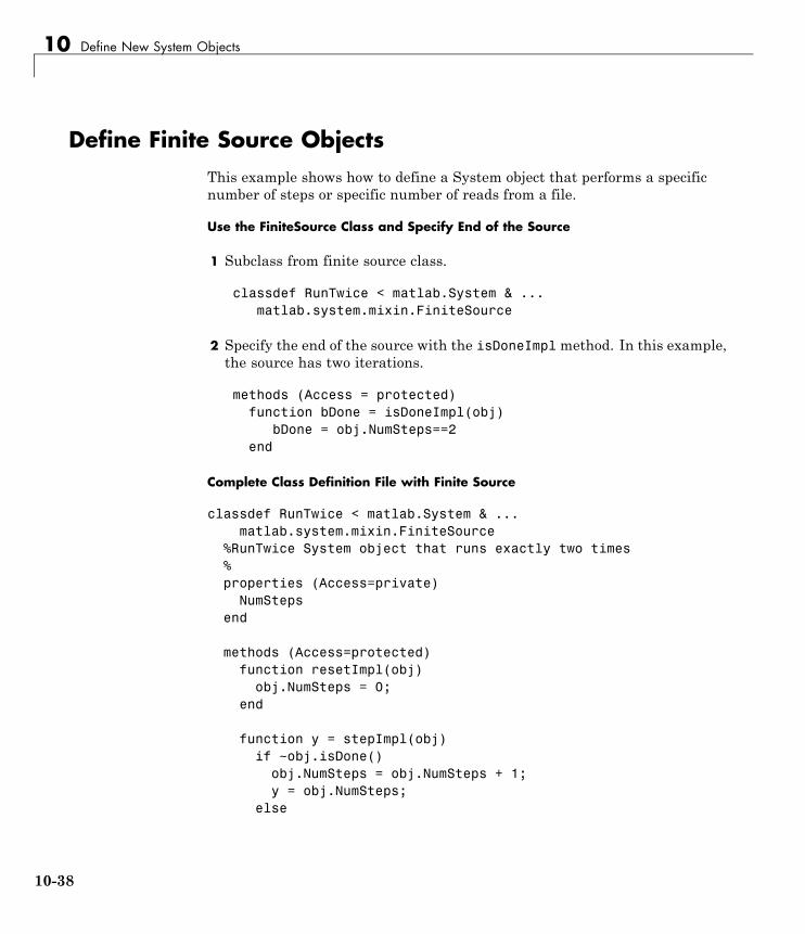
10 Define New System Objects
Define Finite Source ObjectsThis example shows how to define a System object that performs a specificnumber of steps or specific number of reads from a file.
Use the FiniteSource Class and Specify End of the Source
1 Subclass from finite source class.
classdef RunTwice < matlab.System & ...matlab.system.mixin.FiniteSource
2 Specify the end of the source with the isDoneImplmethod. In this example,the source has two iterations.
methods (Access = protected)function bDone = isDoneImpl(obj)
bDone = obj.NumSteps==2end
Complete Class Definition File with Finite Source
classdef RunTwice < matlab.System & ...matlab.system.mixin.FiniteSource
%RunTwice System object that runs exactly two times%properties (Access=private)
NumStepsend
methods (Access=protected)function resetImpl(obj)
obj.NumSteps = 0;end
function y = stepImpl(obj)if ~obj.isDone()
obj.NumSteps = obj.NumSteps + 1;y = obj.NumSteps;
else
10-38

Define Finite Source Objects
y = 0;end
end
function bDone = isDoneImpl(obj)bDone = obj.NumSteps==2;
endend
methods (Access=protected)function n = getNumInputsImpl(~)
n = 0;endfunction n = getNumOutputsImpl(~)
n = 1;end
end
end
See Also matlab.system.mixin.FiniteSource
Concepts • “What Are Mixin Classes?” on page 10-79• “Subclassing Multiple Classes”• “System Object Input Arguments and ~ in Code Examples” on page 10-78
10-39
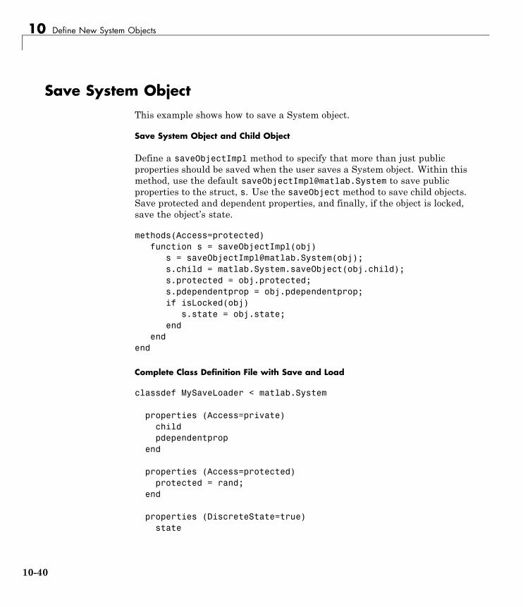
10 Define New System Objects
Save System ObjectThis example shows how to save a System object.
Save System Object and Child Object
Define a saveObjectImpl method to specify that more than just publicproperties should be saved when the user saves a System object. Within thismethod, use the default [email protected] to save publicproperties to the struct, s. Use the saveObject method to save child objects.Save protected and dependent properties, and finally, if the object is locked,save the object’s state.
methods(Access=protected)function s = saveObjectImpl(obj)
s = [email protected](obj);s.child = matlab.System.saveObject(obj.child);s.protected = obj.protected;s.pdependentprop = obj.pdependentprop;if isLocked(obj)
s.state = obj.state;end
endend
Complete Class Definition File with Save and Load
classdef MySaveLoader < matlab.System
properties (Access=private)childpdependentprop
end
properties (Access=protected)protected = rand;
end
properties (DiscreteState=true)state
10-40
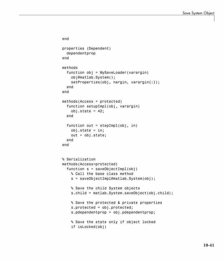
Save System Object
end
properties (Dependent)dependentprop
end
methodsfunction obj = MySaveLoader(varargin)
[email protected]();setProperties(obj, nargin, varargin{:});
endend
methods(Access = protected)function setupImpl(obj, varargin)
obj.state = 42;end
function out = stepImpl(obj, in)obj.state = in;out = obj.state;
endend
% Serializationmethods(Access=protected)
function s = saveObjectImpl(obj)% Call the base class methods = [email protected](obj);
% Save the child System objectss.child = matlab.System.saveObject(obj.child);
% Save the protected & private propertiess.protected = obj.protected;s.pdependentprop = obj.pdependentprop;
% Save the state only if object lockedif isLocked(obj)
10-41
10 Define New System Objects
s.state = obj.state;end
end
function loadObjectImpl(obj,s,wasLocked)% Load child System objectsobj.child = matlab.System.loadObject(s.child);
% Load protected and private propertiesobj.protected = s.protected;obj.pdependentprop = s.pdependentprop;
% Load the state only if object lockedif wasLocked
obj.state = s.state;end
% Call base class method to load public [email protected](obj,s,wasLocked);
endend
end
See Also saveObjectImpl | loadObjectImpl
RelatedExamples
• “Load System Object” on page 10-43
10-42
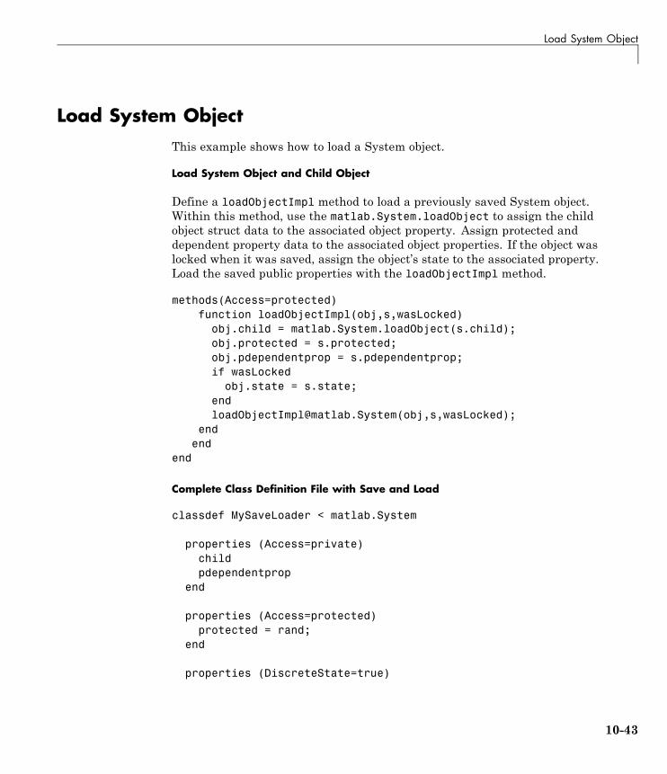
Load System Object
Load System ObjectThis example shows how to load a System object.
Load System Object and Child Object
Define a loadObjectImpl method to load a previously saved System object.Within this method, use the matlab.System.loadObject to assign the childobject struct data to the associated object property. Assign protected anddependent property data to the associated object properties. If the object waslocked when it was saved, assign the object’s state to the associated property.Load the saved public properties with the loadObjectImpl method.
methods(Access=protected)function loadObjectImpl(obj,s,wasLocked)
obj.child = matlab.System.loadObject(s.child);obj.protected = s.protected;obj.pdependentprop = s.pdependentprop;if wasLocked
obj.state = s.state;[email protected](obj,s,wasLocked);
endend
end
Complete Class Definition File with Save and Load
classdef MySaveLoader < matlab.System
properties (Access=private)childpdependentprop
end
properties (Access=protected)protected = rand;
end
properties (DiscreteState=true)
10-43
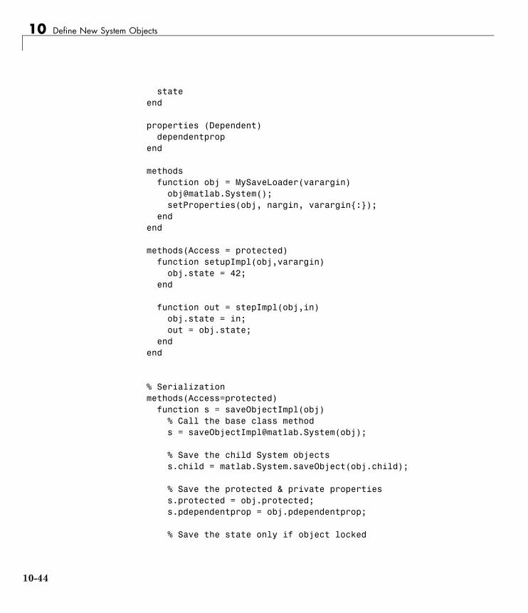
10 Define New System Objects
stateend
properties (Dependent)dependentprop
end
methodsfunction obj = MySaveLoader(varargin)
[email protected]();setProperties(obj, nargin, varargin{:});
endend
methods(Access = protected)function setupImpl(obj,varargin)
obj.state = 42;end
function out = stepImpl(obj,in)obj.state = in;out = obj.state;
endend
% Serializationmethods(Access=protected)
function s = saveObjectImpl(obj)% Call the base class methods = [email protected](obj);
% Save the child System objectss.child = matlab.System.saveObject(obj.child);
% Save the protected & private propertiess.protected = obj.protected;s.pdependentprop = obj.pdependentprop;
% Save the state only if object locked
10-44
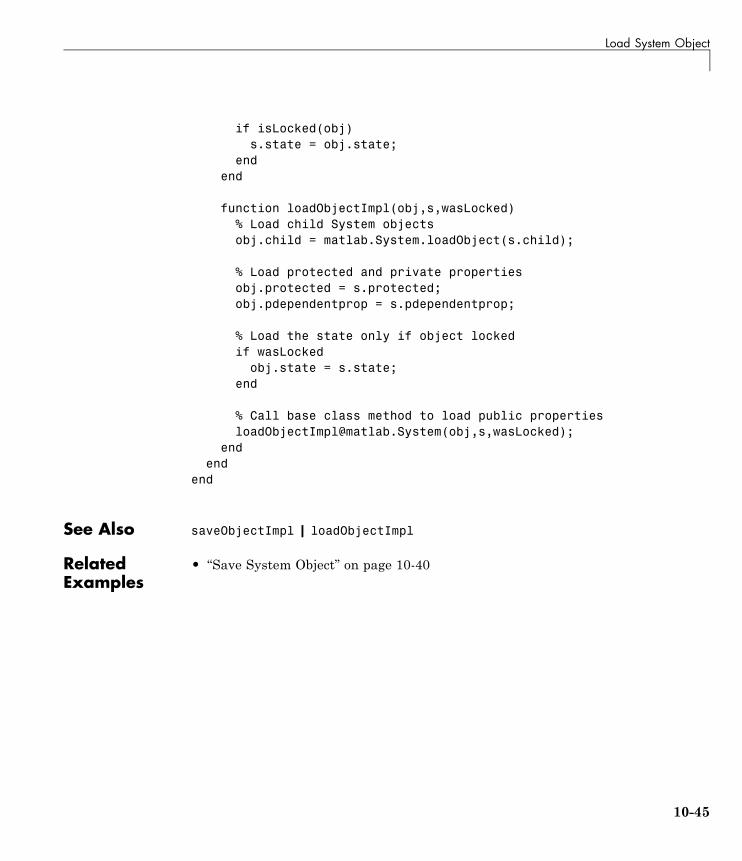
Load System Object
if isLocked(obj)s.state = obj.state;
endend
function loadObjectImpl(obj,s,wasLocked)% Load child System objectsobj.child = matlab.System.loadObject(s.child);
% Load protected and private propertiesobj.protected = s.protected;obj.pdependentprop = s.pdependentprop;
% Load the state only if object lockedif wasLocked
obj.state = s.state;end
% Call base class method to load public [email protected](obj,s,wasLocked);
endend
end
See Also saveObjectImpl | loadObjectImpl
RelatedExamples
• “Save System Object” on page 10-40
10-45
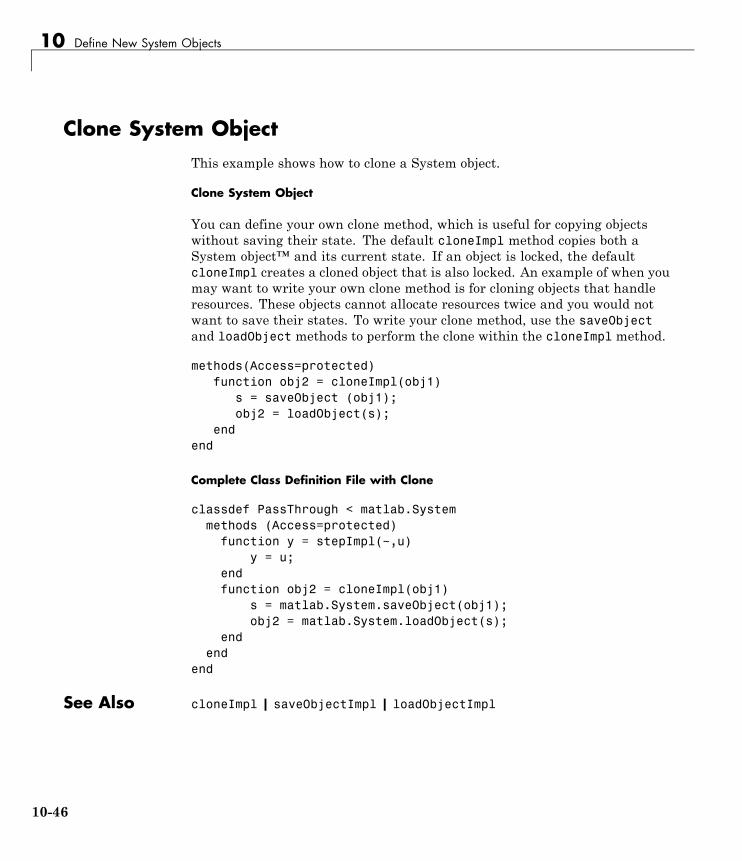
10 Define New System Objects
Clone System ObjectThis example shows how to clone a System object.
Clone System Object
You can define your own clone method, which is useful for copying objectswithout saving their state. The default cloneImpl method copies both aSystem object™ and its current state. If an object is locked, the defaultcloneImpl creates a cloned object that is also locked. An example of when youmay want to write your own clone method is for cloning objects that handleresources. These objects cannot allocate resources twice and you would notwant to save their states. To write your clone method, use the saveObjectand loadObject methods to perform the clone within the cloneImpl method.
methods(Access=protected)function obj2 = cloneImpl(obj1)
s = saveObject (obj1);obj2 = loadObject(s);
endend
Complete Class Definition File with Clone
classdef PassThrough < matlab.Systemmethods (Access=protected)
function y = stepImpl(~,u)y = u;
endfunction obj2 = cloneImpl(obj1)
s = matlab.System.saveObject(obj1);obj2 = matlab.System.loadObject(s);
endend
end
See Also cloneImpl | saveObjectImpl | loadObjectImpl
10-46
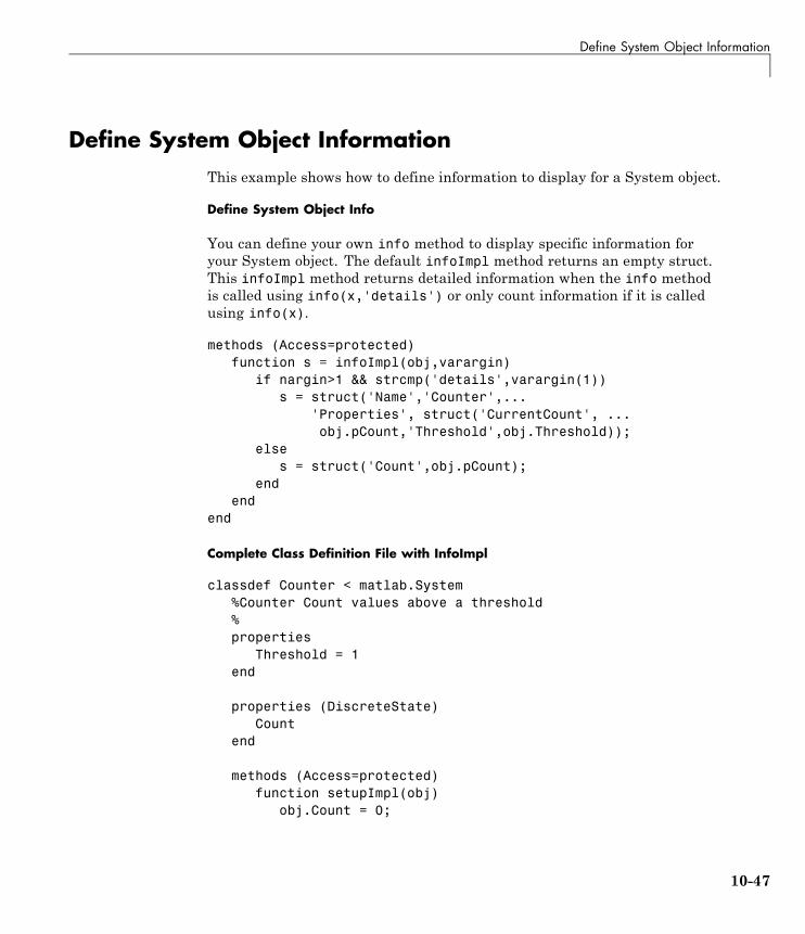
Define System Object Information
Define System Object InformationThis example shows how to define information to display for a System object.
Define System Object Info
You can define your own info method to display specific information foryour System object. The default infoImpl method returns an empty struct.This infoImpl method returns detailed information when the info methodis called using info(x,'details') or only count information if it is calledusing info(x).
methods (Access=protected)function s = infoImpl(obj,varargin)
if nargin>1 && strcmp('details',varargin(1))s = struct('Name','Counter',...
'Properties', struct('CurrentCount', ...obj.pCount,'Threshold',obj.Threshold));
elses = struct('Count',obj.pCount);
endend
end
Complete Class Definition File with InfoImpl
classdef Counter < matlab.System%Counter Count values above a threshold%properties
Threshold = 1end
properties (DiscreteState)Count
end
methods (Access=protected)function setupImpl(obj)
obj.Count = 0;
10-47

10 Define New System Objects
end
function resetImpl(obj)obj.Count = 0;
end
function y = stepImpl(obj, u)if (u > obj.Threshold)
obj.Count = obj.Count + 1;endy = obj.Count;
end
function s = infoImpl(obj,varargin)if nargin>1 && strcmp('details',varargin(1))
s = struct('Name','Counter',...'Properties', struct('CurrentCount', ...obj.pCount,'Threshold',obj.Threshold));
elses = struct('Count',obj.pCount);
endend
end
See Also infoImpl
10-48
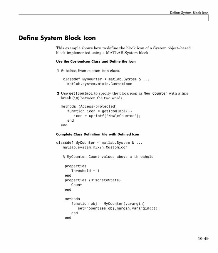
Define System Block Icon
Define System Block IconThis example shows how to define the block icon of a System object–basedblock implemented using a MATLAB System block.
Use the CustomIcon Class and Define the Icon
1 Subclass from custom icon class.
classdef MyCounter < matlab.System & ...matlab.system.mixin.CustomIcon
2 Use getIconImpl to specify the block icon as New Counter with a linebreak (\n) between the two words.
methods (Access=protected)function icon = getIconImpl(~)
icon = sprintf('New\nCounter');end
end
Complete Class Definition File with Defined Icon
classdef MyCounter < matlab.System & ...matlab.system.mixin.CustomIcon
% MyCounter Count values above a threshold
propertiesThreshold = 1
endproperties (DiscreteState)
Countend
methodsfunction obj = MyCounter(varargin)
setProperties(obj,nargin,varargin{:});end
end
10-49

10 Define New System Objects
methods (Access=protected)function setupImpl(obj, u)
obj.Count = 0;endfunction resetImpl(obj)
obj.Count = 0;endfunction y = stepImpl(obj, u)
if (u > obj.Threshold)obj.Count = obj.Count + 1;
endy = obj.Count;
endfunction icon = getIconImpl(~)
icon = sprintf('New\nCounter');end
endend
See Also getIconImpl | matlab.system.mixin.CustomIcon
Concepts • “What Are Mixin Classes?” on page 10-79• “Subclassing Multiple Classes”• “System Object Input Arguments and ~ in Code Examples” on page 10-78
10-50
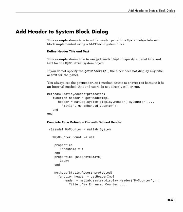
Add Header to System Block Dialog
Add Header to System Block DialogThis example shows how to add a header panel to a System object–basedblock implemented using a MATLAB System block.
Define Header Title and Text
This example shows how to use getHeaderImpl to specify a panel title andtext for the MyCounter System object.
If you do not specify the getHeaderImpl, the block does not display any titleor text for the panel.
You always set the getHeaderImpl method access to protected because it isan internal method that end users do not directly call or run.
methods(Static,Access=protected)function header = getHeaderImpl
header = matlab.system.display.Header('MyCounter',...'Title','My Enhanced Counter');
endend
Complete Class Definition File with Defined Header
classdef MyCounter < matlab.System
%MyCounter Count values
propertiesThreshold = 1
endproperties (DiscreteState)
Countend
methods(Static,Access=protected)function header = getHeaderImpl
header = matlab.system.display.Header('MyCounter',...'Title','My Enhanced Counter',...
10-51
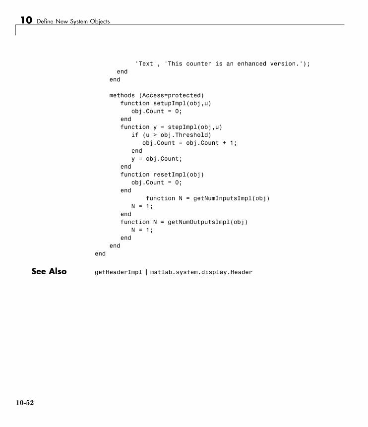
10 Define New System Objects
'Text', 'This counter is an enhanced version.');end
end
methods (Access=protected)function setupImpl(obj,u)
obj.Count = 0;endfunction y = stepImpl(obj,u)
if (u > obj.Threshold)obj.Count = obj.Count + 1;
endy = obj.Count;
endfunction resetImpl(obj)
obj.Count = 0;end
function N = getNumInputsImpl(obj)N = 1;
endfunction N = getNumOutputsImpl(obj)
N = 1;end
endend
See Also getHeaderImpl | matlab.system.display.Header
10-52

Add Property Groups to System Object and Block Dialog
Add Property Groups to System Object and Block DialogThis example shows how to define property sections and section groups forSystem object display. The sections and section groups display as panels andtabs, respectively, in the MATLAB System block dialog.
Define Section of Properties
This example shows how to use matlab.system.display.Section andgetPropertyGroupsImpl to define two property group sections by specifyingtheir titles and property lists.
If you do not specify a property in getPropertyGroupsImpl, the block doesnot display that property.
methods(Static,Access=protected)function groups = getPropertyGroupsImpl
valueGroup = matlab.system.display.Section(...'Title','Value parameters',...'PropertyList',{'StartValue','EndValue'});
thresholdGroup = matlab.system.display.Section(...'Title','Threshold parameters',...'PropertyList',{'Threshold','UseThreshold'});
groups = [valueGroup,thresholdGroup];end
end
Define Group of Sections
This example shows how to use matlab.system.display.SectionGroup,matlab.system.display.Section, and getPropertyGroupsImpl to definetwo tabs, each containing specific properties.
methods(Static,Access=protected)function groups = getPropertyGroupsImpl
upperGroup = matlab.system.display.Section(...'Title', 'Upper threshold', ...'PropertyList',{'UpperThreshold'});
lowerGroup = matlab.system.display.Section(...
10-53
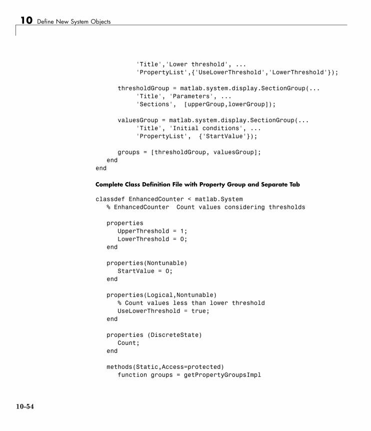
10 Define New System Objects
'Title','Lower threshold', ...'PropertyList',{'UseLowerThreshold','LowerThreshold'});
thresholdGroup = matlab.system.display.SectionGroup(...'Title', 'Parameters', ...'Sections', [upperGroup,lowerGroup]);
valuesGroup = matlab.system.display.SectionGroup(...'Title', 'Initial conditions', ...'PropertyList', {'StartValue'});
groups = [thresholdGroup, valuesGroup];end
end
Complete Class Definition File with Property Group and Separate Tab
classdef EnhancedCounter < matlab.System% EnhancedCounter Count values considering thresholds
propertiesUpperThreshold = 1;LowerThreshold = 0;
end
properties(Nontunable)StartValue = 0;
end
properties(Logical,Nontunable)% Count values less than lower thresholdUseLowerThreshold = true;
end
properties (DiscreteState)Count;
end
methods(Static,Access=protected)function groups = getPropertyGroupsImpl
10-54
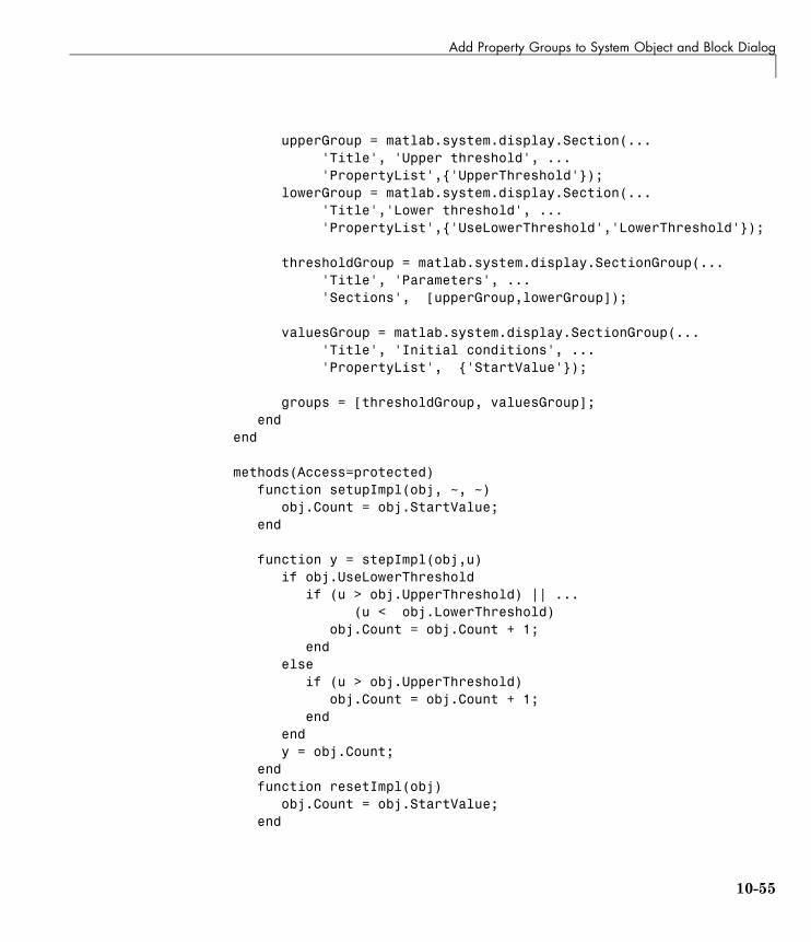
Add Property Groups to System Object and Block Dialog
upperGroup = matlab.system.display.Section(...'Title', 'Upper threshold', ...'PropertyList',{'UpperThreshold'});
lowerGroup = matlab.system.display.Section(...'Title','Lower threshold', ...'PropertyList',{'UseLowerThreshold','LowerThreshold'});
thresholdGroup = matlab.system.display.SectionGroup(...'Title', 'Parameters', ...'Sections', [upperGroup,lowerGroup]);
valuesGroup = matlab.system.display.SectionGroup(...'Title', 'Initial conditions', ...'PropertyList', {'StartValue'});
groups = [thresholdGroup, valuesGroup];end
end
methods(Access=protected)function setupImpl(obj, ~, ~)
obj.Count = obj.StartValue;end
function y = stepImpl(obj,u)if obj.UseLowerThreshold
if (u > obj.UpperThreshold) || ...(u < obj.LowerThreshold)
obj.Count = obj.Count + 1;end
elseif (u > obj.UpperThreshold)
obj.Count = obj.Count + 1;end
endy = obj.Count;
endfunction resetImpl(obj)
obj.Count = obj.StartValue;end
10-55
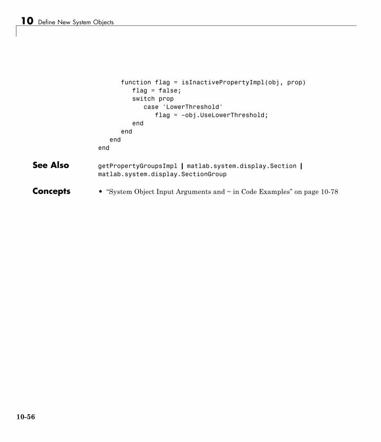
10 Define New System Objects
function flag = isInactivePropertyImpl(obj, prop)flag = false;switch prop
case 'LowerThreshold'flag = ~obj.UseLowerThreshold;
endend
endend
See Also getPropertyGroupsImpl | matlab.system.display.Section |matlab.system.display.SectionGroup
Concepts • “System Object Input Arguments and ~ in Code Examples” on page 10-78
10-56
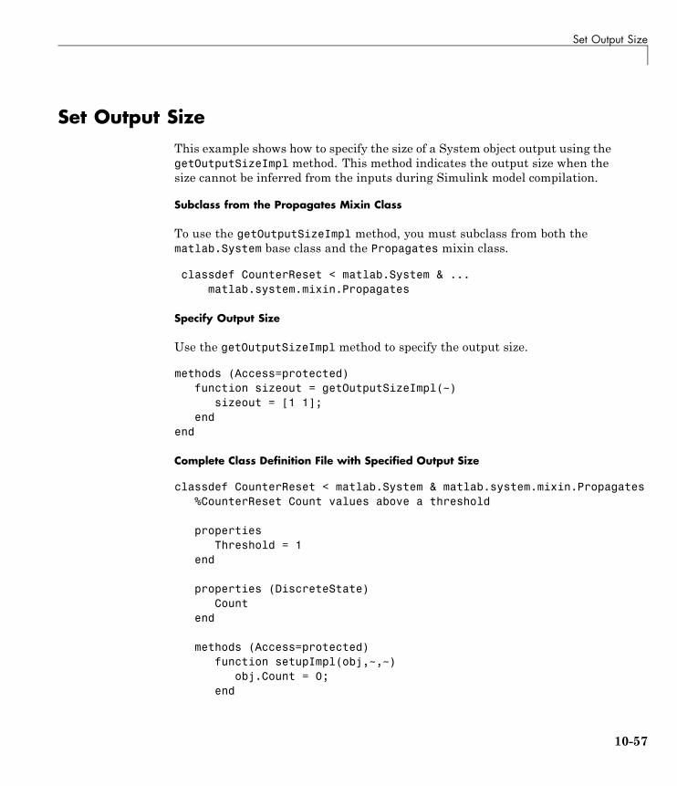
Set Output Size
Set Output SizeThis example shows how to specify the size of a System object output using thegetOutputSizeImpl method. This method indicates the output size when thesize cannot be inferred from the inputs during Simulink model compilation.
Subclass from the Propagates Mixin Class
To use the getOutputSizeImpl method, you must subclass from both thematlab.System base class and the Propagates mixin class.
classdef CounterReset < matlab.System & ...matlab.system.mixin.Propagates
Specify Output Size
Use the getOutputSizeImpl method to specify the output size.
methods (Access=protected)function sizeout = getOutputSizeImpl(~)
sizeout = [1 1];end
end
Complete Class Definition File with Specified Output Size
classdef CounterReset < matlab.System & matlab.system.mixin.Propagates%CounterReset Count values above a threshold
propertiesThreshold = 1
end
properties (DiscreteState)Count
end
methods (Access=protected)function setupImpl(obj,~,~)
obj.Count = 0;end
10-57

10 Define New System Objects
function y = stepImpl(obj,u1,u2)% Add to count if u1 is above threshold% Reset if u2 is trueif (u2)
obj.Count = 0;elseif (u1 > obj.Threshold)
obj.Count = obj.Count + 1;endy = obj.Count;
end
function resetImpl(obj)obj.Count = 0;
end
function N = getNumInputsImpl(~)N = 2;
end
function [sz,dt,cp] = getDiscreteStateSpecificationImpl(~,name)if strcmp(name,'Count')
sz = [1 1];dt = 'double';cp = false;
elseerror(['Error: Incorrect State Name: 'name'.']);
endendfunction dataout = getOutputDataTypeImpl(~)
dataout = 'double';endfunction sizeout = getOutputSizeImpl(~)
sizeout = [1 1];endfunction cplxout = isOutputComplexImpl(~)
cplxout = false;endfunction fixedout = isOutputFixedSizeImpl(~)
fixedout = true;
10-58

Set Output Size
endend
end
See Also matlab.system.mixin.Propagates | getOutputSizeImpl
Concepts • “What Are Mixin Classes?” on page 10-79• “Subclassing Multiple Classes”• “System Object Input Arguments and ~ in Code Examples” on page 10-78
10-59

10 Define New System Objects
Set Output Data TypeThis example shows how to specify the data type of a System object outputusing the getOutputDataTypeImpl method. This method indicates the datatype of the output when the data type cannot be inferred from the inputsduring Simulink model compilation.
Subclass from the Propagates Mixin Class
To use the getOutputDataTypeImpl method, you must subclass from thePropagates mixin class.
classdef CounterReset < matlab.System & ...matlab.system.mixin.Propagates
Specify Output Data Type
Use the getOutputDataTypeImpl method to specify the output data typeas a double.
methods (Access=protected)function dataout = getOutputDataTypeImpl(~)
dataout = 'double';end
end
Complete Class Definition File with Specified Output Data Type
classdef CounterReset < matlab.System & matlab.system.mixin.Propagates%CounterReset Count values above a threshold
propertiesThreshold = 1
end
properties (DiscreteState)Count
end
methods (Access=protected)function setupImpl(obj,~,~)
10-60
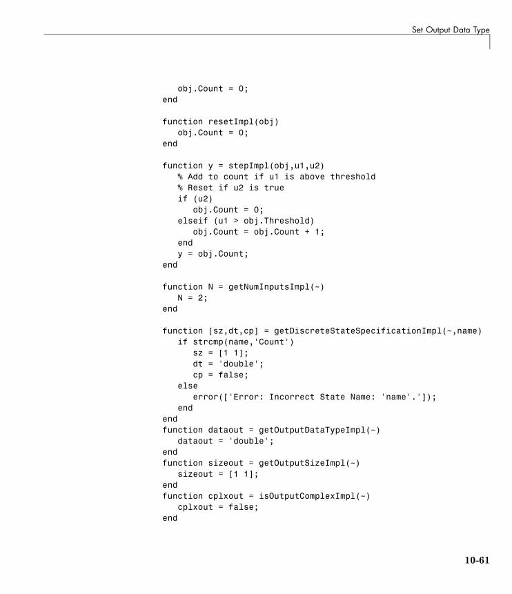
Set Output Data Type
obj.Count = 0;end
function resetImpl(obj)obj.Count = 0;
end
function y = stepImpl(obj,u1,u2)% Add to count if u1 is above threshold% Reset if u2 is trueif (u2)
obj.Count = 0;elseif (u1 > obj.Threshold)
obj.Count = obj.Count + 1;endy = obj.Count;
end
function N = getNumInputsImpl(~)N = 2;
end
function [sz,dt,cp] = getDiscreteStateSpecificationImpl(~,name)if strcmp(name,'Count')
sz = [1 1];dt = 'double';cp = false;
elseerror(['Error: Incorrect State Name: 'name'.']);
endendfunction dataout = getOutputDataTypeImpl(~)
dataout = 'double';endfunction sizeout = getOutputSizeImpl(~)
sizeout = [1 1];endfunction cplxout = isOutputComplexImpl(~)
cplxout = false;end
10-61
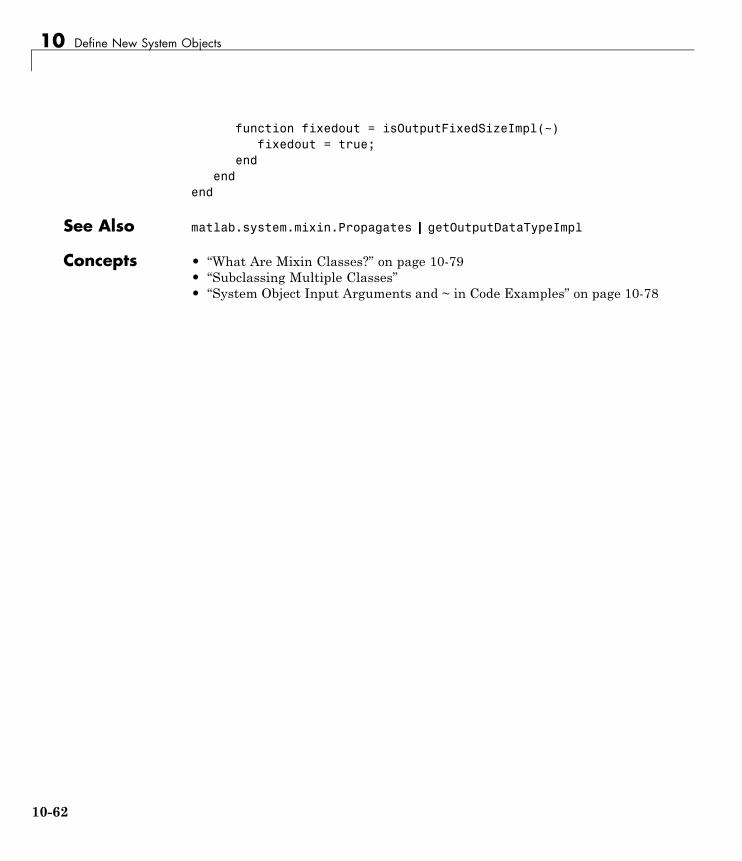
10 Define New System Objects
function fixedout = isOutputFixedSizeImpl(~)fixedout = true;
endend
end
See Also matlab.system.mixin.Propagates | getOutputDataTypeImpl
Concepts • “What Are Mixin Classes?” on page 10-79• “Subclassing Multiple Classes”• “System Object Input Arguments and ~ in Code Examples” on page 10-78
10-62

Set Output Complexity
Set Output ComplexityThis example shows how to specify whether a System object output is acomplex or real value. You use the isOutputComplexImpl method when theoutput complexity cannot be inferred from the inputs during Simulink modelcompilation.
Subclass from the Propagates Mixin Class
To use the isOutputComplexImpl method, you must subclass from both thematlab.System base class and the Propagates mixin class.
classdef CounterReset < matlab.System & ...matlab.system.mixin.Propagates
Specify Output Complexity
Use the isOutputComplexImpl method to specify that the output is real.
methods (Access=protected)function cplxout = isOutputComplexImpl(~)
cplxout = false;end
end
Complete Class Definition File with Specified Complexity
classdef CounterReset < matlab.System & matlab.system.mixin.Propagates%CounterReset Count values above a threshold
propertiesThreshold = 1
end
properties (DiscreteState)Count
end
methods (Access=protected)function setupImpl(obj,~,~)
obj.Count = 0;
10-63
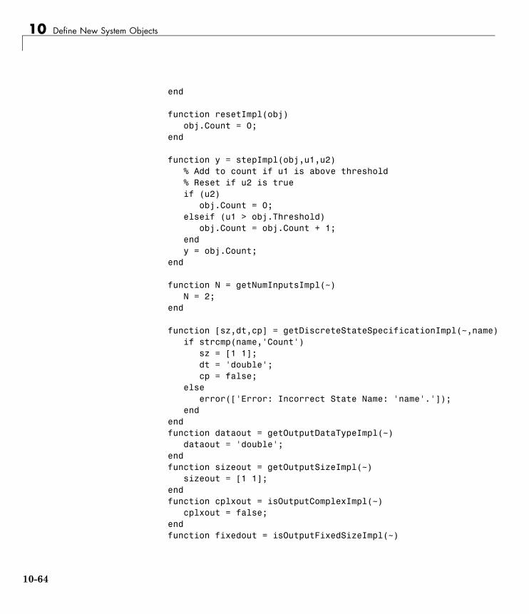
10 Define New System Objects
end
function resetImpl(obj)obj.Count = 0;
end
function y = stepImpl(obj,u1,u2)% Add to count if u1 is above threshold% Reset if u2 is trueif (u2)
obj.Count = 0;elseif (u1 > obj.Threshold)
obj.Count = obj.Count + 1;endy = obj.Count;
end
function N = getNumInputsImpl(~)N = 2;
end
function [sz,dt,cp] = getDiscreteStateSpecificationImpl(~,name)if strcmp(name,'Count')
sz = [1 1];dt = 'double';cp = false;
elseerror(['Error: Incorrect State Name: 'name'.']);
endendfunction dataout = getOutputDataTypeImpl(~)
dataout = 'double';endfunction sizeout = getOutputSizeImpl(~)
sizeout = [1 1];endfunction cplxout = isOutputComplexImpl(~)
cplxout = false;endfunction fixedout = isOutputFixedSizeImpl(~)
10-64

Set Output Complexity
fixedout = true;end
endend
See Also matlab.system.mixin.Propagates | isOutputComplexImpl
Concepts • “What Are Mixin Classes?” on page 10-79• “Subclassing Multiple Classes”• “System Object Input Arguments and ~ in Code Examples” on page 10-78
10-65

10 Define New System Objects
Specify Whether Output Is Fixed- or Variable-SizeThis example shows how to specify whether a System object output has fixed-or variable-size output. . You use the isOutputFixedSizeImpl method whenthe output type cannot be inferred from the inputs during Simulink modelcompilation.
Subclass from the Propagates Mixin Class
To use the isOutputFixedSizeImpl method, you must subclass from both thematlab.System base class and the Propagates mixin class.
classdef CounterReset < matlab.System & ...matlab.system.mixin.Propagates
Specify Output as Fixed Size
Use the isOutputFixedSizeImpl method to specify that the output is fixedsize.
methods (Access=protected)function fixedout = isOutputFixedSizeImpl(~)
fixedout = true;end
end
Complete Class Definition File with Specified Output Data Type
classdef CounterReset < matlab.System & matlab.system.mixin.Propagates%CounterReset Count values above a threshold
propertiesThreshold = 1
end
properties (DiscreteState)Count
end
methods (Access=protected)function setupImpl(obj,~,~)
10-66

Specify Whether Output Is Fixed- or Variable-Size
obj.Count = 0;end
function resetImpl(obj)obj.Count = 0;
end
function y = stepImpl(obj,u1,u2)% Add to count if u1 is above threshold% Reset if u2 is trueif (u2)
obj.Count = 0;elseif (u1 > obj.Threshold)
obj.Count = obj.Count + 1;endy = obj.Count;
end
function N = getNumInputsImpl(~)N = 2;
end
function [sz,dt,cp] = getDiscreteStateSpecificationImpl(~,name)if strcmp(name,'Count')
sz = [1 1];dt = 'double';cp = false;
elseerror(['Error: Incorrect State Name: 'name'.']);
endendfunction dataout = getOutputDataTypeImpl(~)
dataout = 'double';endfunction sizeout = getOutputSizeImpl(~)
sizeout = [1 1];endfunction cplxout = isOutputComplexImpl(~)
cplxout = false;end
10-67

10 Define New System Objects
function fixedout = isOutputFixedSizeImpl(~)fixedout = true;
endend
end
See Also matlab.system.mixin.Propagates | isOutputFixedSizeImpl
Concepts • “What Are Mixin Classes?” on page 10-79• “Subclassing Multiple Classes”• “System Object Input Arguments and ~ in Code Examples” on page 10-78
10-68
Specify Discrete State Output Specification
Specify Discrete State Output SpecificationThis example shows how to specify the size, data type, andcomplexity of a discrete state property. You must use thegetDiscreteStateSpecificationImpl method when your System object hasa property that is defined with the DiscreteState attribute. This methodindicates the output specifications when those specifications cannot beinferred during Simulink model compilation.
Subclass from the Propagates Mixin Class
To use the getDiscreteStateSpecificationImpl method, you must subclassfrom both the matlab.System base class and from the Propagatesmixin class.
classdef CounterReset < matlab.System & ...matlab.system.mixin.Propagates
Specify Discrete State Output Specification
Use the getDiscreteStateSpecificationImpl method to specify the sizeand data type. Also specify the complexity of a discrete state property, whichis used in the counter reset example.
methods (Access=protected)function [sz,dt,cp] = getDiscreteStateSpecificationImpl(~,name)
sz = [1 1];dt = 'double';cp = false;
endend
Complete Class Definition File with Discrete State Output Specification
classdef CounterReset < matlab.System & matlab.system.mixin.Propagates%CounterReset Count values above a threshold
propertiesThreshold = 1
end
properties (DiscreteState)
10-69

10 Define New System Objects
Countend
methods (Access=protected)function setupImpl(obj,~,~)
obj.Count = 0;end
function resetImpl(obj)obj.Count = 0;
end
function y = stepImpl(obj,u1,u2)% Add to count if u1 is above threshold% Reset if u2 is trueif (u2)
obj.Count = 0;elseif (u1 > obj.Threshold)
obj.Count = obj.Count + 1;endy = obj.Count;
end
function N = getNumInputsImpl(~)N = 2;
end
function [sz,dt,cp] = getDiscreteStateSpecificationImpl(~,name)sz = [1 1];dt = 'double';cp = false;
endfunction dataout = getOutputDataTypeImpl(~)
dataout = 'double';endfunction sizeout = getOutputSizeImpl(~)
sizeout = [1 1];endfunction cplxout = isOutputComplexImpl(~)
cplxout = false;
10-70

Specify Discrete State Output Specification
endfunction fixedout = isOutputFixedSizeImpl(~)
fixedout = true;end
endend
See Also matlab.system.mixin.Propagates | getDiscreteStateSpecificationImpl
Concepts • “What Are Mixin Classes?” on page 10-79• “Subclassing Multiple Classes”• “System Object Input Arguments and ~ in Code Examples” on page 10-78
10-71

10 Define New System Objects
Use Update and Output for Nondirect FeedthroughThis example shows how to implement nondirect feedthroughfor a System object using the updateImpl, outputImpl andisInputDirectFeedthroughImpl methods. In nondirect feedthrough, theobject’s outputs depend only on the internal states and properties of theobject, rather than the input at that instant in time. You use these methods toseparate the output calculation from the state updates of a System object. Thisenables you to use that object in a feedback loop and prevent algebraic loops.
Subclass from the Nondirect Mixin Class
To use the updateImpl, outputImpl, and isInputDirectFeedthroughImplmethods, you must subclass from both the matlab.System base class andthe Nondirect mixin class.
classdef IntegerDelaySysObj < matlab.System & ...matlab.system.mixin.Nondirect
Implement Updates to the Object
Implement an updateImpl method to update the object with previous inputs.
methods(Access=protected)function updateImpl(obj,u)
obj.PreviousInput = [u obj.PreviousInput(1:end-1)];end
end
Implenent Outputs from Object
Implement an outputImpl method to output the previous, not the currentinput.
methods(Access=protected)function [y] = outputImpl(obj, ~)
y = obj.PreviousInput(end);end
end
Implement Whether Input Is Direct Feedthrough
10-72

Use Update and Output for Nondirect Feedthrough
Implement an isInputDirectFeedthroughImpl method to indicate that theinput is nondirect feedthrough.
methods(Access=protected)function flag = isInputDirectFeedthroughImpl(~,~)
flag = false;end
end
Complete Class Definition File with Update and Output
classdef intDelaySysObj < matlab.System &...matlab.system.mixin.Nondirect &...matlab.system.mixin.CustomIcon
%intDelaySysObj Delay input by specified number of samples.
propertiesInitialOutput = 0;
endproperties (Nontunable)
NumDelays = 1;endproperties(DiscreteState)
PreviousInput;end
methods(Access=protected)function validatePropertiesImpl(obj)
if ((numel(obj.NumDelays)>1) || (obj.NumDelays <= 0))error('Number of delays must be positive non-zero scalar value.
endif (numel(obj.InitialOutput)>1)
error('Initial Output must be scalar value.');end
end
function setupImpl(obj, ~)obj.PreviousInput = ones(1,obj.NumDelays)*obj.InitialOutput;
end
function resetImpl(obj)
10-73

10 Define New System Objects
obj.PreviousInput = ones(1,obj.NumDelays)*obj.InitialOutput;end
function [y] = outputImpl(obj, ~)y = obj.PreviousInput(end);
endfunction updateImpl(obj, u)
obj.PreviousInput = [u obj.PreviousInput(1:end-1)];endfunction flag = isInputDirectFeedthroughImpl(~,~)
flag = false;end
endend
See Also matlab.system.mixin.Nondirect | outputImpl | updateImpl |isInputDirectFeedthroughImpl
Concepts • “What Are Mixin Classes?” on page 10-79• “Subclassing Multiple Classes”• “System Object Input Arguments and ~ in Code Examples” on page 10-78
10-74
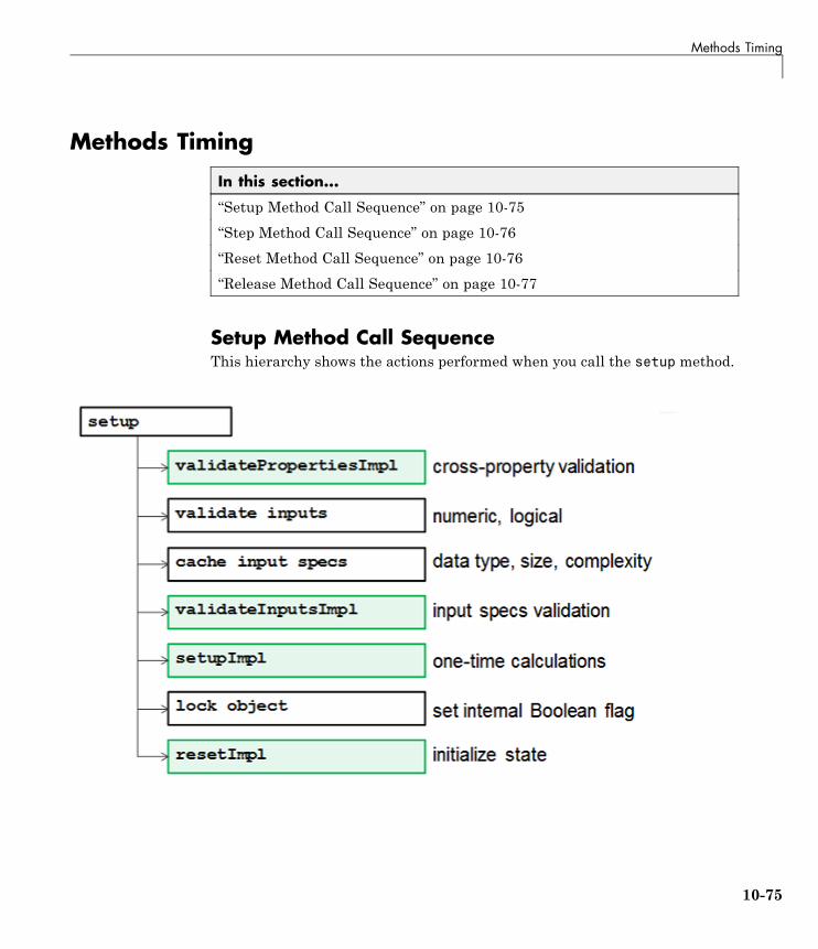
Methods Timing
Methods Timing
In this section...
“Setup Method Call Sequence” on page 10-75
“Step Method Call Sequence” on page 10-76
“Reset Method Call Sequence” on page 10-76
“Release Method Call Sequence” on page 10-77
Setup Method Call SequenceThis hierarchy shows the actions performed when you call the setup method.
10-75

10 Define New System Objects
Step Method Call SequenceThis hierarchy shows the actions performed when you call the step method.
Reset Method Call SequenceThis hierarchy shows the actions performed when you call the reset method.
10-76
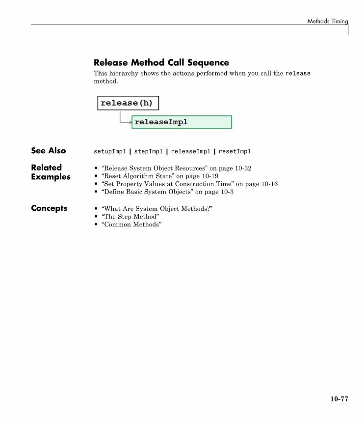
Methods Timing
Release Method Call SequenceThis hierarchy shows the actions performed when you call the releasemethod.
See Also setupImpl | stepImpl | releaseImpl | resetImpl
RelatedExamples
• “Release System Object Resources” on page 10-32• “Reset Algorithm State” on page 10-19• “Set Property Values at Construction Time” on page 10-16• “Define Basic System Objects” on page 10-3
Concepts • “What Are System Object Methods?”• “The Step Method”• “Common Methods”
10-77

10 Define New System Objects
System Object Input Arguments and ~ in Code ExamplesAll methods, except static methods, expect the System object handle as thefirst input argument. You can use any name for your System object handle. Inmany examples, instead of passing in the object handle, ~ is used to indicatethat the object handle is not used in the function. Using ~ instead of an objecthandle prevents warnings about unused variables.
10-78

What Are Mixin Classes?
What Are Mixin Classes?Mixin classes are partial classes that you can combine in various combinationsto form desired behaviors using multiple inheritance. System objects arecomposed of a base class, matlab.System and may include one or more mixinclasses. You specify the base class and mixin classes on the first line of yourclass definition file.
The following mixin classes are available for use with System objects.
• matlab.system.mixin.CustomIcon — Defines a block icon for Systemobjects in the MATLAB System block
• matlab.system.mixin.FiniteSource — Adds the isDone method toSystem objects that are sources
• matlab.system.mixin.Nondirect— Allows the System object, when usedin the MATLAB System block, to support nondirect feedthrough by makingthe runtime callback functions, output and update available
• matlab.system.mixin.Propagates— Enables System objects to operatein the MATLAB System block using the interpreted execution
10-79

10 Define New System Objects
Best Practices for Defining System ObjectsSystem objects are optimized for iterative processing. Use System objectswhen you need to call the step method multiple times or process data in aloop. When defining your own System object, use the following suggestions toensure that your code runs efficiently.
• Define all one-time calculations in the setupImpl method and cache theresults in a private property. Use the stepImpl method for calculationsthat are repeated.
• Define parameters that should not change in a locked object as Nontunableproperties.
• If the number of System object inputs and outputs does not change or ifyou explicitly list the inputs and outputs in the stepImpl method insteadof using varargin or varargout, you do not need to implement thegetNumInputsImpl method.
• Variables that do not need to retain their values between calls and areused in setupImpl, stepImpl, or any other single method should havelocal scope for that method.
• Properties that are accessed more than once in the stepImpl or updateImpland outputImpl methods should be cached as local variables inside thatmethod. Iterative calculations using cached local variables run faster thancalculations that must access the object’s properties. When the stepImplcalculations complete, you can save the local cached results back to theSystem object’s properties. You should copy frequently used tunableproperties into private properties.
For best practices for including System objects in code generation, see “SystemObjects in MATLAB Code Generation”.
10-80

11
Links to Category Pages
• “Signal Management Library” on page 11-2
• “Sinks Library” on page 11-3
• “Math Functions Library” on page 11-4
• “Filtering Library” on page 11-5

11 Links to Category Pages
Signal Management LibraryYou can find the relevant blocks in the following pages:
• “Buffers, Switches, and Counters”
• “Signal Attributes”
• “Signal Operations”
11-2

Sinks Library
Sinks LibraryYou can find the relevant blocks in the following pages:
• “Signal Import and Export”
• “Scopes and Data Logging”
11-3

11 Links to Category Pages
Math Functions LibraryYou can find the relevant blocks in the following pages:
• “Array and Matrix Mathematics”
• “Linear Algebra”
11-4

Filtering Library
Filtering LibraryYou can find the relevant blocks in the following pages:
• “Filter Design”
• “Single-Rate Filters”
• “Multirate and Multistage Filters”
• “Adaptive Filters”
11-5

11 Links to Category Pages
11-6

12
Designing Lowpass FIRFilters
• “Lowpass FIR Filter Design” on page 12-2
• “Controlling Design Specifications in Lowpass FIR Design” on page 12-7
• “Designing Filters with Non-Equiripple Stopband” on page 12-13
• “Minimizing Lowpass FIR Filter Length” on page 12-18
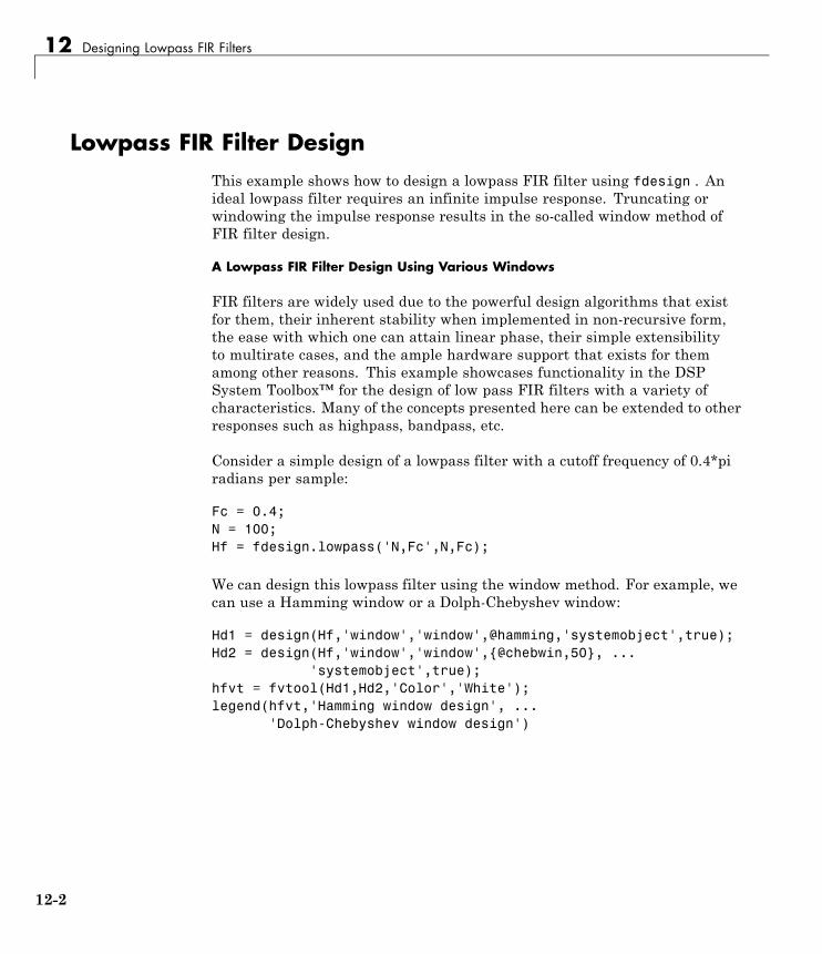
12 Designing Lowpass FIR Filters
Lowpass FIR Filter DesignThis example shows how to design a lowpass FIR filter using fdesign . Anideal lowpass filter requires an infinite impulse response. Truncating orwindowing the impulse response results in the so-called window method ofFIR filter design.
A Lowpass FIR Filter Design Using Various Windows
FIR filters are widely used due to the powerful design algorithms that existfor them, their inherent stability when implemented in non-recursive form,the ease with which one can attain linear phase, their simple extensibilityto multirate cases, and the ample hardware support that exists for themamong other reasons. This example showcases functionality in the DSPSystem Toolbox™ for the design of low pass FIR filters with a variety ofcharacteristics. Many of the concepts presented here can be extended to otherresponses such as highpass, bandpass, etc.
Consider a simple design of a lowpass filter with a cutoff frequency of 0.4*piradians per sample:
Fc = 0.4;N = 100;Hf = fdesign.lowpass('N,Fc',N,Fc);
We can design this lowpass filter using the window method. For example, wecan use a Hamming window or a Dolph-Chebyshev window:
Hd1 = design(Hf,'window','window',@hamming,'systemobject',true);Hd2 = design(Hf,'window','window',{@chebwin,50}, ...
'systemobject',true);hfvt = fvtool(Hd1,Hd2,'Color','White');legend(hfvt,'Hamming window design', ...
'Dolph-Chebyshev window design')
12-2
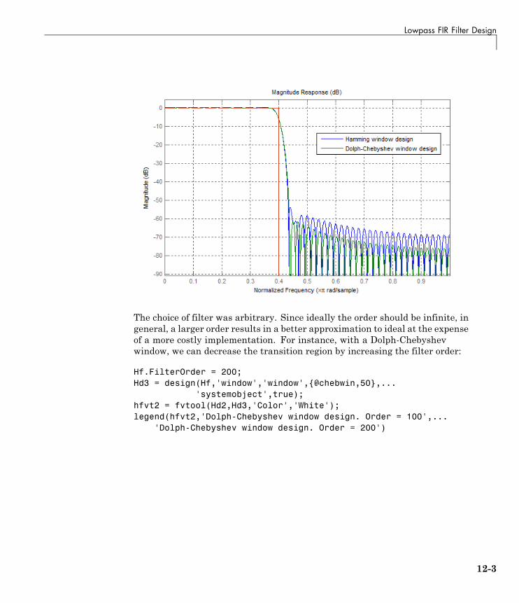
Lowpass FIR Filter Design
The choice of filter was arbitrary. Since ideally the order should be infinite, ingeneral, a larger order results in a better approximation to ideal at the expenseof a more costly implementation. For instance, with a Dolph-Chebyshevwindow, we can decrease the transition region by increasing the filter order:
Hf.FilterOrder = 200;Hd3 = design(Hf,'window','window',{@chebwin,50},...
'systemobject',true);hfvt2 = fvtool(Hd2,Hd3,'Color','White');legend(hfvt2,'Dolph-Chebyshev window design. Order = 100',...
'Dolph-Chebyshev window design. Order = 200')
12-3
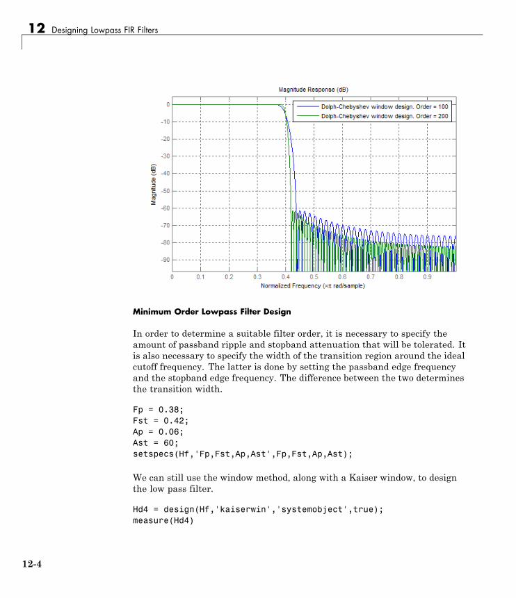
12 Designing Lowpass FIR Filters
Minimum Order Lowpass Filter Design
In order to determine a suitable filter order, it is necessary to specify theamount of passband ripple and stopband attenuation that will be tolerated. Itis also necessary to specify the width of the transition region around the idealcutoff frequency. The latter is done by setting the passband edge frequencyand the stopband edge frequency. The difference between the two determinesthe transition width.
Fp = 0.38;Fst = 0.42;Ap = 0.06;Ast = 60;setspecs(Hf,'Fp,Fst,Ap,Ast',Fp,Fst,Ap,Ast);
We can still use the window method, along with a Kaiser window, to designthe low pass filter.
Hd4 = design(Hf,'kaiserwin','systemobject',true);measure(Hd4)
12-4

Lowpass FIR Filter Design
ans =
Sampling Frequency : N/A (normalized frequency)Passband Edge : 0.383-dB Point : 0.395396-dB Point : 0.4Stopband Edge : 0.42Passband Ripple : 0.016058 dBStopband Atten. : 60.092 dBTransition Width : 0.04
One thing to note is that the transition width as specified is centered aroundthe cutoff frequency of 0.4 pi. This will become the point at which the gain ofthe lowpass filter is half the passband gain (or the point at which the filterreaches 6 dB of attenuation).
Optimal Minimum Order Designs
The Kaiser window design is not an optimal design and as a result the filterorder required to meet the specifications using this method is larger than itneeds to be. Equiripple designs result in the lowpass filter with the smallestpossible order to meet a set of specifications.
Hd5 = design(Hf,'equiripple','systemobject',true);hfvt3 = fvtool(Hd4,Hd5,'Color','White');legend(hfvt3,'Kaiser window design','Equiripple design')
12-5
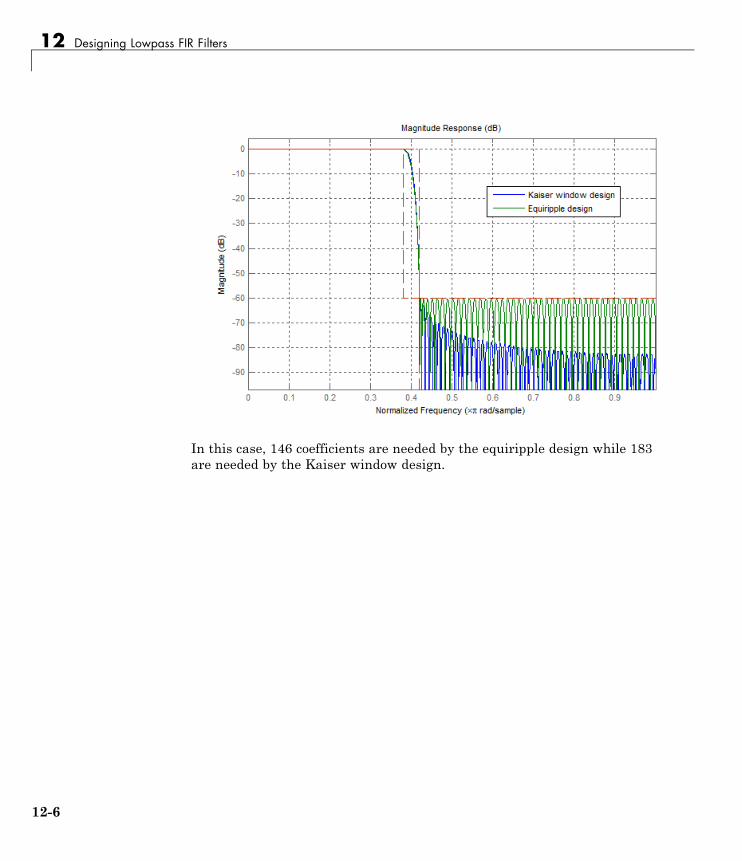
12 Designing Lowpass FIR Filters
In this case, 146 coefficients are needed by the equiripple design while 183are needed by the Kaiser window design.
12-6
Controlling Design Specifications in Lowpass FIR Design
Controlling Design Specifications in Lowpass FIR DesignThis example shows how to control the filter order, passband ripple, stopbandattenuation, and transition region width of a lowpass FIR filter.
Controlling the Filter Order and Passband Ripples and Stopband Attenuation
When targeting custom hardware, it is common to find cases where thenumber of coefficients is constrained to a set number. In these cases,minimum order designs are not useful because there is no control over theresulting filter order. As an example, suppose that only 101 coefficients couldbe used and the passband ripple/stopband attenuation specifications need tobe met. We can still use equiripple designs for these specifications. However,we lose control over the transition width which will increase. This is the priceto pay for reducing the order while maintaining the passband ripple/stopbandattenuation specifications.
Consider a simple design of a lowpass filter with a cutoff frequency of 0.4*piradians per sample:
Ap = 0.06;Ast = 60;Fp = 0.38;Fst = 0.42;Hf=fdesign.lowpass('Fp,Fst,Ap,Ast',Fp,Fst,Ap,Ast);
Design an equiripple filter:
Hd1 = design(Hf,'equiripple','systemobject',true);
Set the number of coefficients to 101, which means setting the order to 100:
N = 100; % order = 100 -> 101 coefficientsFc = 0.4;setspecs(Hf,'N,Fc,Ap,Ast',N,Fc,Ap,Ast);
Design a second equiripple filter with the given constraint:
Hd2 = design(Hf,'equiripple','systemobject',true);
12-7

12 Designing Lowpass FIR Filters
Measure the filter variables of the second equiripple filter, and compare thegraphs of the first and second filters:
measure(Hd2)hfvt = fvtool(Hd1,Hd2,'Color','White');legend(hfvt,'Equiripple design, 146 coeffcients', ...
'Equiripple design, 101 coefficients')
Sampling Frequency : N/A (normalized frequency)Passband Edge : 0.373163-dB Point : 0.392856-dB Point : 0.4Stopband Edge : 0.43134Passband Ripple : 0.06 dBStopband Atten. : 60 dBTransition Width : 0.058177
Notice that the transition has increased by almost 50%. This is not surprisinggiven the almost 50% difference between 101 coefficients and 146 coefficients.
Controlling the Transition Region Width
12-8
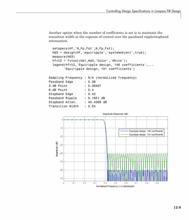
Controlling Design Specifications in Lowpass FIR Design
Another option when the number of coefficients is set is to maintain thetransition width at the expense of control over the passband ripple/stopbandattenuation.
setspecs(Hf,'N,Fp,Fst',N,Fp,Fst);Hd3 = design(Hf,'equiripple','systemobject',true);measure(Hd3)hfvt2 = fvtool(Hd1,Hd3,'Color','White');legend(hfvt2,'Equiripple design, 146 coefficients',...
'Equiripple design, 101 coefficients')
Sampling Frequency : N/A (normalized frequency)Passband Edge : 0.383-dB Point : 0.394076-dB Point : 0.4Stopband Edge : 0.42Passband Ripple : 0.1651 dBStopband Atten. : 40.4369 dBTransition Width : 0.04
12-9
12 Designing Lowpass FIR Filters
Note that in this case, the differences between using 146 coefficients andusing 101 coefficients is reflected in a larger passband ripple and a smallerstopband attenuation.
It is possible to increase the attenuation in the stopband while keeping thesame filter order and transition width by the use of weights. Weights area way of specifying the relative importance of the passband ripple versusthe stopband attenuation. By default, passband and stopband are equallyweighted (a weight of one is assigned to each). If we increase the stopbandweight, we can increase the stopband attenuation at the expense of increasingthe stopband ripple as well.
Hd4 = design(Hf,'equiripple','Wstop',5,'systemobject',true);measure(Hd4)hfvt3 = fvtool(Hd3,Hd4,'Color','White');legend(hfvt3,'Passband weight = 1, Stopband weight = 1',...
'Passband weight = 1, Stopband weight = 5')
Sampling Frequency : N/A (normalized frequency)Passband Edge : 0.383-dB Point : 0.391436-dB Point : 0.39722Stopband Edge : 0.42Passband Ripple : 0.34529 dBStopband Atten. : 48.0068 dBTransition Width : 0.04
12-10

Controlling Design Specifications in Lowpass FIR Design
Another possibility is to specify the exact stopband attenuation desired andlose control over the passband ripple. This is a powerful and very desirablespecification. One has control over most parameters of interest.
setspecs(Hf,'N,Fp,Fst,Ast',N,Fp,Fst,Ast);Hd5 = design(Hf,'equiripple','systemobject',true);hfvt4 = fvtool(Hd4,Hd5,'Color','White');legend(hfvt4,'Equiripple design using weights',...
'Equiripple design constraining the stopband')
12-11

12 Designing Lowpass FIR Filters
12-12
Designing Filters with Non-Equiripple Stopband
Designing Filters with Non-Equiripple StopbandThis example shows how to design lowpass filters with stopbands that arenot equiripple.
Optimal Non-Equiripple Lowpass Filters
To start, set up the filter parameters and use fdesign to create a constructorfor designing the filter.
N = 100;Fp = 0.38;Fst = 0.42;Hf = fdesign.lowpass('N,Fp,Fst',N,Fp,Fst);
Equiripple designs achieve optimality by distributing the deviation fromthe ideal response uniformly. This has the advantage of minimizing themaximum deviation (ripple). However, the overall deviation, measured interms of its energy tends to be large. This may not always be desirable. Whenlow pass filtering a signal, this implies that remnant energy of the signal inthe stopband may be relatively large. When this is a concern, least-squaresmethods provide optimal designs that minimize the energy in the stopband.
Hd1 = design(Hf,'equiripple','systemobject',true);Hd2 = design(Hf,'firls','systemobject',true);hfvt = fvtool(Hd1,Hd2,'Color','White');legend(hfvt,'Equiripple design','Least-squares design')
12-13
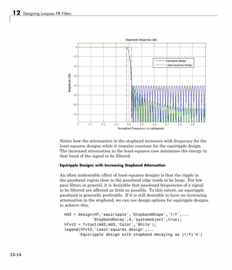
12 Designing Lowpass FIR Filters
Notice how the attenuation in the stopband increases with frequency for theleast-squares designs while it remains constant for the equiripple design.The increased attenuation in the least-squares case minimizes the energy inthat band of the signal to be filtered.
Equiripple Designs with Increasing Stopband Attenuation
An often undesirable effect of least-squares designs is that the ripple inthe passband region close to the passband edge tends to be large. For lowpass filters in general, it is desirable that passband frequencies of a signalto be filtered are affected as little as possible. To this extent, an equiripplepassband is generally preferable. If it is still desirable to have an increasingattenuation in the stopband, we can use design options for equiripple designsto achieve this.
Hd3 = design(Hf,'equiripple','StopbandShape','1/f',...'StopbandDecay',4,'systemobject',true);
hfvt2 = fvtool(Hd2,Hd3,'Color','White');legend(hfvt2,'Least-squares design',...
'Equiripple design with stopband decaying as (1/f)^4')
12-14

Designing Filters with Non-Equiripple Stopband
Notice that the stopbands are quite similar. However the equiripple designhas a significantly smaller passband ripple,
mls = measure(Hd2);meq = measure(Hd3);mls.Apassmeq.Apass
ans =
0.3504
ans =
0.1867
Filters with a stopband that decays as (1/f)^M will decay at 6M dB per octave.Another way of shaping the stopband is using a linear decay. For example
12-15
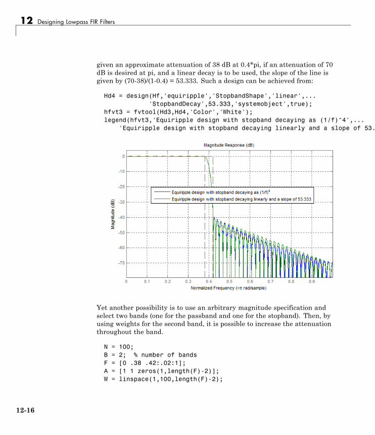
12 Designing Lowpass FIR Filters
given an approximate attenuation of 38 dB at 0.4*pi, if an attenuation of 70dB is desired at pi, and a linear decay is to be used, the slope of the line isgiven by (70-38)/(1-0.4) = 53.333. Such a design can be achieved from:
Hd4 = design(Hf,'equiripple','StopbandShape','linear',...'StopbandDecay',53.333,'systemobject',true);
hfvt3 = fvtool(Hd3,Hd4,'Color','White');legend(hfvt3,'Equiripple design with stopband decaying as (1/f)^4',...
'Equiripple design with stopband decaying linearly and a slope of 53.
Yet another possibility is to use an arbitrary magnitude specification andselect two bands (one for the passband and one for the stopband). Then, byusing weights for the second band, it is possible to increase the attenuationthroughout the band.
N = 100;B = 2; % number of bandsF = [0 .38 .42:.02:1];A = [1 1 zeros(1,length(F)-2)];W = linspace(1,100,length(F)-2);
12-16

Designing Filters with Non-Equiripple Stopband
Harb = fdesign.arbmag('N,B,F,A',N,B,F(1:2),A(1:2),F(3:end),...A(3:end));
Ha = design(Harb,'equiripple','B2Weights',W,...'systemobject',true);
fvtool(Ha,'Color','White')
12-17

12 Designing Lowpass FIR Filters
Minimizing Lowpass FIR Filter LengthThis example shows how to minimize the number coefficients, by designingminimum-phase or minimum-order filters.
Minimum-Phase Lowpass Filter Design
To start, set up the filter parameters and use fdesign to create a constructorfor designing the filter.
N = 100;Fp = 0.38;Fst = 0.42;Ap = 0.06;Ast = 60;Hf = fdesign.lowpass('Fp,Fst,Ap,Ast',Fp,Fst,Ap,Ast);
So far, we have only considered linear-phase designs. Linear phase isdesirable in many applications. Nevertheless, if linear phase is not arequirement, minimum-phase designs can provide significant improvementsover linear phase counterparts. For instance, returning to the minimum ordercase, a minimum-phase/minimum-order design for the same specificationscan be computed with:
Hd1 = design(Hf,'equiripple','systemobject',true);Hd2 = design(Hf,'equiripple','minphase',true,...
'systemobject',true);hfvt = fvtool(Hd1,Hd2,'Color','White');legend(hfvt,'Linear-phase equiripple design',...
'Minimum-phase equiripple design')
12-18
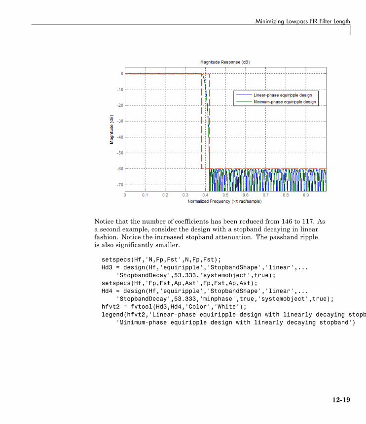
Minimizing Lowpass FIR Filter Length
Notice that the number of coefficients has been reduced from 146 to 117. Asa second example, consider the design with a stopband decaying in linearfashion. Notice the increased stopband attenuation. The passband rippleis also significantly smaller.
setspecs(Hf,'N,Fp,Fst',N,Fp,Fst);Hd3 = design(Hf,'equiripple','StopbandShape','linear',...
'StopbandDecay',53.333,'systemobject',true);setspecs(Hf,'Fp,Fst,Ap,Ast',Fp,Fst,Ap,Ast);Hd4 = design(Hf,'equiripple','StopbandShape','linear',...
'StopbandDecay',53.333,'minphase',true,'systemobject',true);hfvt2 = fvtool(Hd3,Hd4,'Color','White');legend(hfvt2,'Linear-phase equiripple design with linearly decaying stopb
'Minimum-phase equiripple design with linearly decaying stopband')
12-19

12 Designing Lowpass FIR Filters
Minimum-Order Lowpass Filter Design Using Multistage Techniques
A different approach to minimizing the number of coefficients that does notinvolve minimum-phase designs is to use multistage techniques. Here weshow an interpolated FIR (IFIR) approach.
Hd5 = ifir(Hf);hfvt3 = fvtool(Hd1,Hd5,'Color','White');legend(hfvt3,'Linear-phase equirriple design',...
'Linear-phase IFIR design')
12-20

Minimizing Lowpass FIR Filter Length
The number of nonzero coefficients required in the IFIR case is 111. Less thanboth the equiripple linear-phase and minimum-phase designs.
12-21

12 Designing Lowpass FIR Filters
12-22

13
FDATool: A Filter Designand Analysis GUI
• “Overview” on page 13-2
• “Using FDATool” on page 13-6
• “Importing a Filter Design” on page 13-39

13 FDATool: A Filter Design and Analysis GUI
Overview
In this section...
“FDATool” on page 13-2
“Filter Design Methods” on page 13-2
“Using the Filter Design and Analysis Tool” on page 13-4
“Analyzing Filter Responses” on page 13-4
“Filter Design and Analysis Tool Panels” on page 13-4
“Getting Help” on page 13-5
FDAToolThe Filter Design and Analysis Tool (FDATool) is a user interface fordesigning and analyzing filters quickly. FDATool enables you to design digitalFIR or IIR filters by setting filter specifications, by importing filters fromyour MATLAB workspace, or by adding, moving or deleting poles and zeros.FDATool also provides tools for analyzing filters, such as magnitude andphase response and pole-zero plots.
Filter Design MethodsFDATool gives you access to the following Signal Processing Toolbox filterdesign methods.
Design Method Function
Butterworth butter
Chebyshev Type I cheby1
Chebyshev Type II cheby2
Elliptic ellip
Maximally Flat maxflat
Equiripple firpm
Least-squares firls
13-2

Overview
Design Method Function
Constrained least-squares fircls
Complex equiripple cfirpm
Window fir1
When using the window method in FDATool, all Signal Processing Toolboxwindow functions are available, and you can specify a user-defined window byentering its function name and input parameter.
Advanced Filter Design MethodsThe following advanced filter design methods are available if you have DSPSystem Toolbox software.
Design Method Function
Constrained equiripple FIR firceqrip
Constrained-band equiripple FIR fircband
Generalized remez FIR firgr
Equripple halfband FIR firhalfband
Least P-norm optimal FIR firlpnorm
Equiripple Nyquist FIR firnyquist
Interpolated FIR ifir
IIR comb notching or peaking iircomb
Allpass filter (given group delay) iirgrpdelay
Least P-norm optimal IIR iirlpnorm
Constrained least P-norm IIR iirlpnormc
Second-order IIR notch iirnotch
Second-order IIR peaking (resonator) iirpeak
13-3

13 FDATool: A Filter Design and Analysis GUI
Using the Filter Design and Analysis ToolThere are different ways that you can design filters using the Filter Designand Analysis Tool. For example:
• You can first choose a response type, such as bandpass, and then choosefrom the available FIR or IIR filter design methods.
• You can specify the filter by its type alone, along with certain frequency-or time-domain specifications such as passband frequencies and stopbandfrequencies. The filter you design is then computed using the default filterdesign method and filter order.
Analyzing Filter ResponsesOnce you have designed your filter, you can display the filter coefficientsand detailed filter information, export the coefficients to the MATLABworkspace, and create a C header file containing the coefficients, and analyzedifferent filter responses in FDATool or in a separate Filter Visualization Tool(fvtool). The following filter responses are available:
• Magnitude response (freqz)
• Phase response (phasez)
• Group delay (grpdelay)
• Phase delay (phasedelay)
• Impulse response (impz)
• Step response (stepz)
• Pole-zero plots (zplane)
• Zero-phase response (zerophase)
Filter Design and Analysis Tool PanelsThe Filter Design and Analysis Tool has sidebar buttons that displayparticular panels in the lower half of the tool. The panels are
• Design Filter. See “Choosing a Filter Design Method” on page 13-8 for moreinformation. You use this panel to
- Design filters from scratch.
13-4
Overview
- Modify existing filters designed in FDATool.
- Analyze filters.
• Import filter. You use this panel to
- Import previously saved filters or filter coefficients that you have storedin the MATLAB workspace.
- Analyze imported filters.
• Pole/Zero Editor. See “Editing the Filter Using the Pole/Zero Editor” onpage 13-19. You use this panel to add, delete, and move poles and zerosin your filter design.
If you also have DSP System Toolbox product installed, additional panelsare available:
• Set quantization parameters — Use this panel to quantize double-precisionfilters that you design in FDATool, quantize double-precision filters thatyou import into FDATool, and analyze quantized filters.
• Transform filter — Use this panel to change a filter from one responsetype to another.
• Multirate filter design — Use this panel to create a multirate filterfrom your existing FIR design, create CIC filters, and linear and holdinterpolators.
If you have Simulink installed, this panel is available:
• Realize Model — Use this panel to create a Simulink block containing thefilter structure.
Getting Help
At any time, you can right-click or click theWhat’s this? button, , to getinformation on the different parts of the tool. You can also use the Helpmenu to see complete Help information.
13-5

13 FDATool: A Filter Design and Analysis GUI
Using FDAToolTo open FDATool, type
fdatool
at the MATLAB command prompt.
The Filter Design and Analysis Tool opens with the Design Filter paneldisplayed.
Note that when you open FDATool, Design Filter is not enabled. You mustmake a change to the default filter design in order to enable Design Filter.This is true each time you want to change the filter design. Changes toradio button items or drop down menu items such as those under ResponseType or Filter Order enable Design Filter immediately. Changes tospecifications in text boxes such as Fs, Fpass, and Fstop require you to clickoutside the text box to enable Design Filter.
13-6

Using FDATool
Choosing a Response TypeYou can choose from several response types:
• Lowpass
• Raised cosine
• Highpass
• Bandpass
• Bandstop
• Differentiator
• Multiband
• Hilbert transformer
• Arbitrary magnitude
Additional response types are available if you have DSP System Toolboxsoftware installed.
To design a bandpass filter, select the radio button next to Bandpass inthe Response Type region of the GUI.
Note Not all filter design methods are available for all response types. Onceyou choose your response type, this may restrict the filter design methodsavailable to you. Filter design methods that are not available for a selectedresponse type are removed from the Design Method region of the GUI.
13-7

13 FDATool: A Filter Design and Analysis GUI
Choosing a Filter Design MethodYou can use the default filter design method for the response type that you’veselected, or you can select a filter design method from the available FIR andIIR methods listed in the GUI.
To select the Remez algorithm to compute FIR filter coefficients, select theFIR radio button and choose Equiripple from the list of methods.
Setting the Filter Design Specifications
• “Viewing Filter Specifications” on page 13-8
• “Filter Order” on page 13-9
• “Options” on page 13-9
• “Bandpass Filter Frequency Specifications” on page 13-10
• “Bandpass Filter Magnitude Specifications” on page 13-12
Viewing Filter SpecificationsThe filter design specifications that you can set vary according to responsetype and design method. The display region illustrates filter specificationswhen you select Analysis > Filter Specifications or when you click theFilter Specifications toolbar button.
You can also view the filter specifications on the Magnitude plot of a designedfilter by selecting View > Specification Mask.
13-8

Using FDATool
Filter OrderYou have two mutually exclusive options for determining the filter orderwhen you design an equiripple filter:
• Specify order: You enter the filter order in a text box.
• Minimum order: The filter design method determines the minimumorder filter.
Select the Minimum order radio button for this example.
Note that filter order specification options depend on the filter design methodyou choose. Some filter methods may not have both options available.
OptionsThe available options depend on the selected filter design method. Onlythe FIR Equiripple and FIR Window design methods have settable options.
13-9

13 FDATool: A Filter Design and Analysis GUI
For FIR Equiripple, the option is a Density Factor. See firpm for moreinformation. For FIR Window the options are Scale Passband, Windowselection, and for the following windows, a settable parameter:
Window Parameter
Chebyshev (chebwin) Sidelobe attenuation
Gaussian (gausswin) Alpha
Kaiser (kaiser) Beta
Taylor (taylorwin) Nbar and Sidelobe level
Tukey (tukeywin) Alpha
User Defined Function Name, Parameter
You can view the window in the Window Visualization Tool (wvtool) byclicking the View button.
For this example, set the Density factor to 16.
Bandpass Filter Frequency SpecificationsFor a bandpass filter, you can set
• Units of frequency:
- Hz
- kHz
- MHz
- Normalized (0 to 1)
13-10

Using FDATool
• Sampling frequency
• Passband frequencies
• Stopband frequencies
You specify the passband with two frequencies. The first frequencydetermines the lower edge of the passband, and the second frequencydetermines the upper edge of the passband.
Similarly, you specify the stopband with two frequencies. The first frequencydetermines the upper edge of the first stopband, and the second frequencydetermines the lower edge of the second stopband.
For this example:
• Keep the units in Hz (default).
• Set the sampling frequency (Fs) to 2000 Hz.
• Set the end of the first stopband (Fstop1) to 200 Hz.
• Set the beginning of the passband (Fpass1) to 300 Hz.
• Set the end of the passband (Fpass2) to 700 Hz.
• Set the beginning of the second stopband (Fstop2) to 800 Hz.
13-11
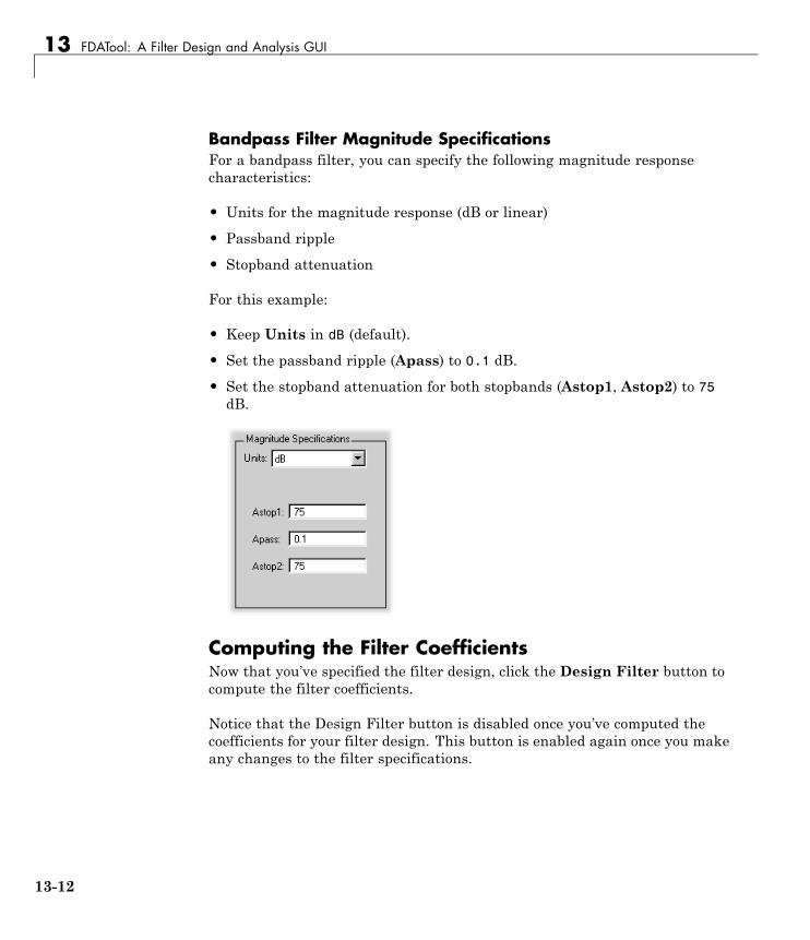
13 FDATool: A Filter Design and Analysis GUI
Bandpass Filter Magnitude SpecificationsFor a bandpass filter, you can specify the following magnitude responsecharacteristics:
• Units for the magnitude response (dB or linear)
• Passband ripple
• Stopband attenuation
For this example:
• Keep Units in dB (default).
• Set the passband ripple (Apass) to 0.1 dB.
• Set the stopband attenuation for both stopbands (Astop1, Astop2) to 75dB.
Computing the Filter CoefficientsNow that you’ve specified the filter design, click the Design Filter button tocompute the filter coefficients.
Notice that the Design Filter button is disabled once you’ve computed thecoefficients for your filter design. This button is enabled again once you makeany changes to the filter specifications.
13-12
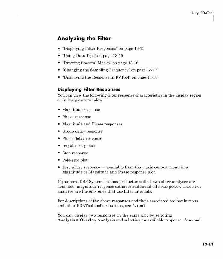
Using FDATool
Analyzing the Filter
• “Displaying Filter Responses” on page 13-13
• “Using Data Tips” on page 13-15
• “Drawing Spectral Masks” on page 13-16
• “Changing the Sampling Frequency” on page 13-17
• “Displaying the Response in FVTool” on page 13-18
Displaying Filter ResponsesYou can view the following filter response characteristics in the display regionor in a separate window.
• Magnitude response
• Phase response
• Magnitude and Phase responses
• Group delay response
• Phase delay response
• Impulse response
• Step response
• Pole-zero plot
• Zero-phase response — available from the y-axis context menu in aMagnitude or Magnitude and Phase response plot.
If you have DSP System Toolbox product installed, two other analyses areavailable: magnitude response estimate and round-off noise power. These twoanalyses are the only ones that use filter internals.
For descriptions of the above responses and their associated toolbar buttonsand other FDATool toolbar buttons, see fvtool.
You can display two responses in the same plot by selectingAnalysis > Overlay Analysis and selecting an available response. A second
13-13

13 FDATool: A Filter Design and Analysis GUI
y-axis is added to the right side of the response plot. (Note that not allresponses can be overlaid on each other.)
You can also display the filter coefficients and detailed filter information inthis region.
For all the analysis methods, except zero-phase response, you can accessthem from the Analysis menu, the Analysis Parameters dialog box from thecontext menu, or by using the toolbar buttons. For zero-phase, right-click they-axis of the plot and select Zero-phase from the context menu.
For example, to look at the filter’s magnitude response, select theMagnitudeResponse button on the toolbar.
You can also overlay the filter specifications on the Magnitude plot byselecting View > Specification Mask.
Note You can use specification masks in FVTool only if FVTool was launchedfrom FDATool.
13-14

Using FDATool
Using Data TipsYou can click the response to add plot data tips that display informationabout particular points on the response.
For information on using data tips, see “Data Cursor — Displaying DataValues Interactively” in the MATLAB documentation.
13-15

13 FDATool: A Filter Design and Analysis GUI
Drawing Spectral MasksTo add spectral masks or rejection area lines to your magnitude plot, clickView > User-defined Spectral Mask.
The mask is defined by a frequency vector and a magnitude vector. Thesevectors must be the same length.
• Enable Mask — Select to turn on the mask display.
• Normalized Frequency — Select to normalize the frequency between 0and 1 across the displayed frequency range.
• Frequency Vector— Enter a vector of x-axis frequency values.
• Magnitude Units — Select the desired magnitude units. These unitsshould match the units used in the magnitude plot.
• Magnitude Vector— Enter a vector of y-axis magnitude values.
The magnitude response below shows a spectral mask.
13-16
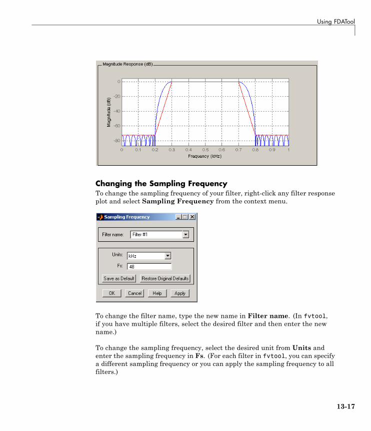
Using FDATool
Changing the Sampling FrequencyTo change the sampling frequency of your filter, right-click any filter responseplot and select Sampling Frequency from the context menu.
To change the filter name, type the new name in Filter name. (In fvtool,if you have multiple filters, select the desired filter and then enter the newname.)
To change the sampling frequency, select the desired unit from Units andenter the sampling frequency in Fs. (For each filter in fvtool, you can specifya different sampling frequency or you can apply the sampling frequency to allfilters.)
13-17
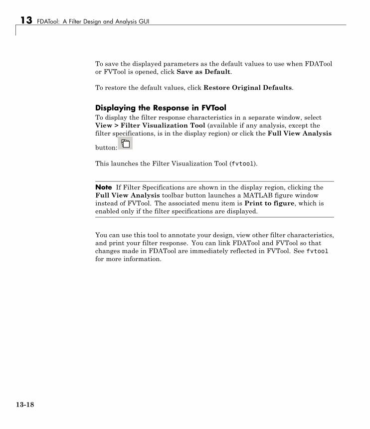
13 FDATool: A Filter Design and Analysis GUI
To save the displayed parameters as the default values to use when FDAToolor FVTool is opened, click Save as Default.
To restore the default values, click Restore Original Defaults.
Displaying the Response in FVToolTo display the filter response characteristics in a separate window, selectView > Filter Visualization Tool (available if any analysis, except thefilter specifications, is in the display region) or click the Full View Analysis
button:
This launches the Filter Visualization Tool (fvtool).
Note If Filter Specifications are shown in the display region, clicking theFull View Analysis toolbar button launches a MATLAB figure windowinstead of FVTool. The associated menu item is Print to figure, which isenabled only if the filter specifications are displayed.
You can use this tool to annotate your design, view other filter characteristics,and print your filter response. You can link FDATool and FVTool so thatchanges made in FDATool are immediately reflected in FVTool. See fvtoolfor more information.
13-18
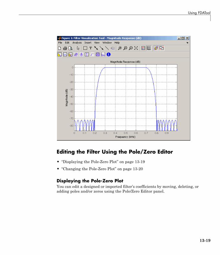
Using FDATool
Editing the Filter Using the Pole/Zero Editor
• “Displaying the Pole-Zero Plot” on page 13-19
• “Changing the Pole-Zero Plot” on page 13-20
Displaying the Pole-Zero PlotYou can edit a designed or imported filter’s coefficients by moving, deleting, oradding poles and/or zeros using the Pole/Zero Editor panel.
13-19

13 FDATool: A Filter Design and Analysis GUI
Note You cannot generate MATLAB code (File > Generate MATLABcode) if your filter was designed or edited with the Pole/Zero Editor.
You cannot move quantized poles and zeros. You can only move the referencepoles and zeros.
Click the Pole/Zero Editor button in the sidebar or select Edit > Pole/ZeroEditor to display this panel.
Poles are shown using x symbols and zeros are shown using o symbols.
Changing the Pole-Zero PlotPlot mode buttons are located to the left of the pole/zero plot. Select one of thebuttons to change the mode of the pole/zero plot. The Pole/Zero Editor has
13-20

Using FDATool
these buttons from left to right: move pole, add pole, add zero, and deletepole or zero.
The following plot parameters and controls are located to the left of thepole/zero plot and below the plot mode buttons.
• Filter gain— factor to compensate for the filter’s pole(s) and zero(s) gains
• Coordinates— units (Polar or Rectangular) of the selected pole or zero
• Magnitude — if polar coordinates is selected, magnitude of the selectedpole or zero
• Angle— if polar coordinates is selected, angle of selected pole(s) or zero(s)
• Real — if rectangular coordinates is selected, real component of selectedpole(s) or zero(s)
• Imaginary— if rectangular coordinates is selected, imaginary componentof selected pole or zero
• Section— for multisection filters, number of the current section
• Conjugate — creates a corresponding conjugate pole or zero orautomatically selects the conjugate pole or zero if it already exists.
• Auto update— immediately updates the displayed magnitude responsewhen poles or zeros are added, moved, or deleted.
The Edit > Pole/Zero Editor has items for selecting multiple poles/zeros,for inverting and mirroring poles/zeros, and for deleting, scaling and rotatingpoles/zeros.
13-21

13 FDATool: A Filter Design and Analysis GUI
Moving one of the zeros on the vertical axis produces the following result:
13-22

Using FDATool
• The selected zero pair is shown in green.
• When you select one of the zeros from a conjugate pair, the Conjugate checkbox and the conjugate are automatically selected.
• The Magnitude Response plot updates immediately because Auto updateis active.
Converting the Filter Structure
• “Converting to a New Structure” on page 13-23
• “Converting to Second-Order Sections” on page 13-25
Converting to a New StructureYou can use Edit > Convert Structure to convert the current filter to a newstructure. All filters can be converted to the following representations:
13-23
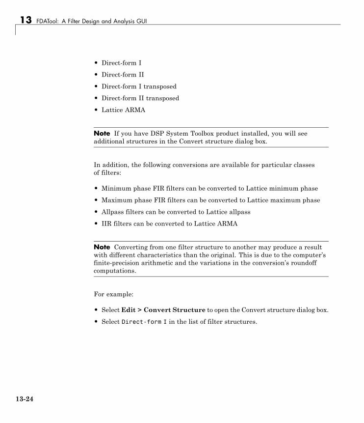
13 FDATool: A Filter Design and Analysis GUI
• Direct-form I
• Direct-form II
• Direct-form I transposed
• Direct-form II transposed
• Lattice ARMA
Note If you have DSP System Toolbox product installed, you will seeadditional structures in the Convert structure dialog box.
In addition, the following conversions are available for particular classesof filters:
• Minimum phase FIR filters can be converted to Lattice minimum phase
• Maximum phase FIR filters can be converted to Lattice maximum phase
• Allpass filters can be converted to Lattice allpass
• IIR filters can be converted to Lattice ARMA
Note Converting from one filter structure to another may produce a resultwith different characteristics than the original. This is due to the computer’sfinite-precision arithmetic and the variations in the conversion’s roundoffcomputations.
For example:
• Select Edit > Convert Structure to open the Convert structure dialog box.
• Select Direct-form I in the list of filter structures.
13-24
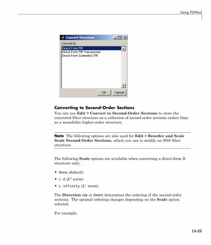
Using FDATool
Converting to Second-Order SectionsYou can use Edit > Convert to Second-Order Sections to store theconverted filter structure as a collection of second-order sections rather thanas a monolithic higher-order structure.
Note The following options are also used for Edit > Reorder and ScaleScale Second-Order Sections, which you use to modify an SOS filterstructure.
The following Scale options are available when converting a direct-form IIstructure only:
• None (default)
• L-2 (L2 norm)
• L-infinity (L∞ norm)
The Direction (Up or Down) determines the ordering of the second-ordersections. The optimal ordering changes depending on the Scale optionselected.
For example:
13-25

13 FDATool: A Filter Design and Analysis GUI
• Select Edit > Convert to Second-Order Sections to open the Convert toSOS dialog box.
• Select L-infinity from the Scale menu for L∞ norm scaling.
• Leave Up as the Direction option.
Note To convert from second-order sections back to a single section, useEdit > Convert to Single Section.
Exporting a Filter Design
• “Exporting Coefficients or Objects to the Workspace” on page 13-26
• “Exporting Coefficients to an ASCII File” on page 13-27
• “Exporting Coefficients or Objects to a MAT-File” on page 13-28
• “Exporting to SPTool” on page 13-29
• “Exporting to a Simulink Model” on page 13-29
• “Other Ways to Export a Filter” on page 13-32
Exporting Coefficients or Objects to the WorkspaceYou can save the filter either as filter coefficients variables or as a dfilt ormfilt filter object variable. (Note that you must have DSP System Toolboxproduct installed to save as an mfilt.) To save the filter to the MATLABworkspace:
1 Select File > Export. The Export dialog box appears.
2 Select Workspace from the Export To menu.
3 Select Coefficients from the Export As menu to save the filtercoefficients or select Objects to save the filter in a filter object.
4 For coefficients, assign variable names using the Numerator (for FIRfilters) or Numerator and Denominator (for IIR filters), or SOS Matrixand Scale Values (for IIR filters in second-order section form) text boxesin the Variable Names region.
13-26

Using FDATool
For objects, assign the variable name in the Discrete Filter (orQuantized Filter) text box. If you have variables with the same namesin your workspace and you want to overwrite them, select the OverwriteVariables check box.
5 Click the Export button.
Exporting Coefficients to an ASCII FileTo save filter coefficients to a text file,
13-27
13 FDATool: A Filter Design and Analysis GUI
1 Select File > Export. The Export dialog box appears.
2 Select Coefficients File (ASCII) from the Export To menu.
3 Click the Export button. The Export Filter Coefficients to .FCF File dialogbox appears.
4 Choose or enter a filename and click the Save button.
The coefficients are saved in the text file that you specified, and the MATLABEditor opens to display the file. The text file also contains comments with theMATLAB version number, the Signal Processing Toolbox version number,and filter information.
Exporting Coefficients or Objects to a MAT-FileTo save filter coefficients or a filter object as variables in a MAT-file:
1 Select File > Export. The Export dialog box appears.
2 Select MAT-file from the Export To menu.
3 Select Coefficients from the Export As menu to save the filtercoefficients or select Objects to save the filter in a filter object.
4 For coefficients, assign variable names using the Numerator (for FIRfilters) or Numerator and Denominator (for IIR filters), or SOS Matrixand Scale Values (for IIR filters in second-order section form) text boxesin the Variable Names region.
For objects, assign the variable name in the Discrete Filter (orQuantized Filter) text box. If you have variables with the same namesin your workspace and you want to overwrite them, select the OverwriteVariables check box.
5 Click the Export button. The Export to a MAT-File dialog box appears.
6 Choose or enter a filename and click the Save button.
13-28
Using FDATool
Exporting to SPToolYou may want to use your designed filter in SPTool to do signal processingand analysis.
1 Select File > Export. The Export dialog box appears.
2 Select SPTool from the Export To menu.
3 Assign the variable name in the Discrete Filter (or Quantized Filter)text box. If you have variables with the same names in your workspace andyou want to overwrite them, select the Overwrite Variables check box.
4 Click the Export button.
SPTool opens and the current FDATool filter appears in the Filter area listas the specified variable name followed by (Imported).
Note If you are using the DSP System Toolbox software and export aquantized filter, only the values of its quantized coefficients are exported.The reference coefficients are not exported. SPTool does not restrict thecoefficient values, so if you edit them in SPTool by moving poles or zeros,the filter will no longer be in quantized form.
Exporting to a Simulink ModelIf you have the Simulink product installed, you can export a Simulink block ofyour filter design and insert it into a new or existing Simulink model.
You can export a filter designed using any filter design method availablein FDATool.
Note If you have the DSP System Toolbox and Fixed-Point Designerinstalled, you can export a CIC filter to a Simulink model.
1 After designing your filter, click theRealize Model sidebar button or selectFile > Export to Simulink Model. The Realize Model panel is displayed.
13-29

13 FDATool: A Filter Design and Analysis GUI
2 Specify the name to use for your block in Block name.
3 To insert the block into the current (most recently selected) Simulinkmodel, set the Destination to Current. To inset the block into a newmodel, select New. To insert the block into a user-defined subsystem, selectUser defined.
4 If you want to overwrite a block previously created from this panel, checkOverwrite generated ‘Filter’ block.
5 If you select the Build model using basic elements check box, your filteris created as a subsystem block, which uses separate sub-elements. In thismode, the following optimization(s) are available:
• Optimize for zero gains — Removes zero-valued gain paths fromthe filter structure.
• Optimize for unity gains — Substitutes a wire (short circuit) forgains equal to 1 in the filter structure.
• Optimize for negative gains— Substitutes a wire (short circuit) forgains equal to -1 and changes corresponding additions to subtractions inthe filter structure.
• Optimize delay chains— Substitutes delay chains composed of n unitdelays with a single delay of n.
• Optimize for unity scale values — Removes multiplications forscale values equal to 1 from the filter structure.
The following illustration shows the effects of some of the optimizations:
13-30

Using FDATool
Optimization Effects
Note The Build model using basic elements check box is enabledonly when you have a DSP System Toolbox license and your filter can bedesigned using a Digital Filter block. For more information, see the FilterRealization Wizard topic in the DSP System Toolbox documentation.
6 Set the Input processing parameter to specify whether the generatedfilter performs sample- or frame-based processing on the input. Depending
13-31
13 FDATool: A Filter Design and Analysis GUI
on the type of filter you design, one or both of the following options maybe available:
• Columns as channels (frame based)— When you select this option,the block treats each column of the input as a separate channel.
• Elements as channels (sample based) — When you select thisoption, the block treats each element of the input as a separate channel.
7 Click the Realize Model button to create the filter block. When the Buildmodel using basic elements check box is selected, FDATool implementsthe filter as a subsystem block using Sum, Gain, and Delay blocks.
If you double-click the Simulink Filter block, the filter structure is displayed.
Other Ways to Export a FilterYou can also send your filter to a C header file or generate MATLAB code toconstruct your filter from the command line. For detailed instructions, seethe following sections:
• “Generating a C Header File” on page 13-32
• “Generating MATLAB Code” on page 13-34
Generating a C Header FileYou may want to include filter information in an external C program. Tocreate a C header file with variables that contain filter parameter data,follow this procedure:
1 Select Targets > Generate C Header. The Generate C Header dialogbox appears.
13-32

Using FDATool
2 Enter the variable names to be used in the C header file. The particularfilter structure determines the variables that are created in the file
Filter Structure Variable Parameter
Direct-form IDirect-form IIDirect-form ItransposedDirect-form IItransposed
Numerator, Numerator length*, Denominator,Denominator length*, and Number of sections(inactive if filter has only one section)
Lattice ARMA Lattice coeffs, Lattice coeffs length*, Laddercoeffs, Ladder coeffs length*, Number of sections(inactive if filter has only one section)
Lattice MA Lattice coeffs, Lattice coeffs length*, and Numberof sections (inactive if filter has only one section)
Direct-form FIRDirect-form FIRtransposed
Numerator, Numerator length*, and Number ofsections (inactive if filter has only one section)
*length variables contain the total number of coefficients of that type.
13-33
13 FDATool: A Filter Design and Analysis GUI
Note Variable names cannot be C language reserved words, such as “for.”
3 Select Export Suggested to use the suggested data type or select ExportAs and select the desired data type from the pull-down.
Note If you do not have DSP System Toolbox software installed, selectingany data type other than double-precision floating point results in a filterthat does not exactly match the one you designed in the FDATool. This isdue to rounding and truncating differences.
4 Click OK to save the file and close the dialog box or click Apply to save thefile, but leave the dialog box open for additional C header file definitions.
Generating MATLAB CodeYou can generate MATLAB code that constructs the filter you designedin FDATool from the command line. Select File > Generate MATLABCode > Filter Design Function and specify the filename in the GenerateMATLAB code dialog box.
Note You cannot generate MATLAB code (File > Generate MATLABCode > Filter Design Function) if your filter was designed or edited withthe Pole/Zero Editor.
The following is generated MATLAB code for the default lowpass filter inFDATool.
function Hd = ExFilter
%EXFILTER Returns a discrete-time filter object.
%
% MATLAB Code
% Generated by MATLAB(R) 7.11 and the Signal Processing Toolbox 6.14.
%
% Generated on: 17-Feb-2010 14:15:37
13-34

Using FDATool
%
% Equiripple Lowpass filter designed using the FIRPM function.
% All frequency values are in Hz.
Fs = 48000; % Sampling Frequency
Fpass = 9600; % Passband Frequency
Fstop = 12000; % Stopband Frequency
Dpass = 0.057501127785; % Passband Ripple
Dstop = 0.0001; % Stopband Attenuation
dens = 20; % Density Factor
% Calculate the order from the parameters using FIRPMORD.
[N, Fo, Ao, W] = firpmord([Fpass, Fstop]/(Fs/2), [1 0], [Dpass, Dstop]);
% Calculate the coefficients using the FIRPM function.
b = firpm(N, Fo, Ao, W, {dens});
Hd = dfilt.dffir(b);
% [EOF]
Managing Filters in the Current SessionYou can store filters designed in the current FDATool session for cascadingtogether, exporting to FVTool or for recalling later in the same or futureFDATool sessions.
You store and access saved filters with the Store filter and Filter Managerbuttons, respectively, in the Current Filter Information pane.
13-35

13 FDATool: A Filter Design and Analysis GUI
Store Filter — Displays the Store Filter dialog box in which you specify thefilter name to use when storing the filter in the Filter Manager. The defaultname is the type of the filter.
Filter Manager — Opens the Filter Manager.
13-36

Using FDATool
The current filter is listed below the listbox. To change the current filter,highlight the desired filter. If you select Edit current filter, FDATooldisplays the currently selected filter specifications. If you make any changesto the specifications, the stored filter is updated immediately.
To cascade two or more filters, highlight the desired filters and pressCascade. A new cascaded filter is added to the Filter Manager.
To change the name of a stored filter, press Rename. The Rename filterdialog box is displayed.
To remove a stored filter from the Filter Manager, press Delete.
To export one or more filters to FVTool, highlight the filter(s) and pressFVTool.
13-37

13 FDATool: A Filter Design and Analysis GUI
Saving and Opening Filter Design SessionsYou can save your filter design session as a MAT-file and return to the samesession another time.
Select the Save session button to save your session as a MAT-file.The first time you save a session, a Save Filter Design File browser opens,prompting you for a session name.
For example, save this design session as TestFilter.fda in your currentworking directory by typing TestFilter in the File name field.
The .fda extension is added automatically to all filter design sessions yousave.
Note You can also use the File > Save session and File > Save sessionas to save a session.
You can load existing sessions into the Filter Design and Analysis Tool
by selecting the Open session button, or File > Open session . ALoad Filter Design File browser opens that allows you to select from yourpreviously saved filter design sessions.
13-38

Importing a Filter Design
Importing a Filter Design
In this section...
“Import Filter Panel” on page 13-39
“Filter Structures” on page 13-40
Import Filter PanelThe Import Filter panel allows you to import a filter. You can access thisregion by clicking the Import Filter button in the sidebar.
The imported filter can be in any of the representations listed in the FilterStructure pull-down menu. You can import a filter as second-order sectionsby selecting the check box.
Specify the filter coefficients in Numerator and Denominator, eitherby entering them explicitly or by referring to variables in the MATLABworkspace.
Select the frequency units from the following options in the Units menu, andfor any frequency unit other than Normalized, specify the value or MATLABworkspace variable of the sampling frequency in the Fs field.
To import the filter, click the Import Filter button. The display region isautomatically updated when the new filter has been imported.
You can edit the imported filter using the Pole/Zero Editor panel.
13-39
13 FDATool: A Filter Design and Analysis GUI
Filter StructuresThe available filter structures are:
• Direct Form, which includes direct-form I, direct-form II, direct-form Itransposed, direct-form II transposed, and direct-form FIR
• Lattice, which includes lattice allpass, lattice MA min phase, lattice MAmax phase, and lattice ARMA
• Discrete–time Filter (dfilt object)
The structure that you choose determines the type of coefficients that youneed to specify in the text fields to the right.
Direct-formFor direct-form I, direct-form II, direct-form I transposed, and direct-form IItransposed, specify the filter by its transfer function representation
H zb b z b z b m z
a a z a Z
m( )
( ) ( ) ( ) ( )
( ) ( ) ( )
1 2 3 1
1 2 3
1 2
1 3 aa n z n( ) 1
• The Numerator field specifies a variable name or value for the numeratorcoefficient vector b, which contains m+1 coefficients in descending powersof z.
• The Denominator field specifies a variable name or value for thedenominator coefficient vector a, which contains n+1 coefficients indescending powers of z. For FIR filters, the Denominator is 1.
Filters in transfer function form can be produced by all of the SignalProcessing Toolbox filter design functions (such as fir1, fir2, firpm, butter,yulewalk). See “Transfer Function” for more information.
Importing as second-order sections. For all direct-form structures,except direct-form FIR, you can import the filter in its second-order sectionrepresentation:
13-40

Importing a Filter Design
H z Gb b z b z
a a z a zk k k
k k kk
L( )
0 1
12
2
0 11
22
1
The Gain field specifies a variable name or a value for the gain G, and theSOS Matrix field specifies a variable name or a value for the L-by-6 SOSmatrix
SOS
b b b a ab b b a a
b b bL L L
01 11 21 11 22
02 12 22 12 22
0 1 2
11
1
· · · · · ·· · · · · ·
aa aL L1 2
whose rows contain the numerator and denominator coefficients bik and aikof the second-order sections of H(z).
Filters in second-order section form can be produced by functions such astf2sos, zp2sos, ss2sos, and sosfilt. See “Second-Order Sections (SOS)”for more information.
LatticeFor lattice allpass, lattice minimum and maximum phase, and lattice ARMAfilters, specify the filter by its lattice representation:
• For lattice allpass, the Lattice coeff field specifies the lattice (reflection)coefficients, k(1) to k(N), where N is the filter order.
• For lattice MA (minimum or maximum phase), the Lattice coeff fieldspecifies the lattice (reflection) coefficients, k(1) to k(N), where N is thefilter order.
• For lattice ARMA, the Lattice coeff field specifies the lattice (reflection)coefficients, k(1) to k(N), and the Ladder coeff field specifies the laddercoefficients, v(1) to v(N+1), where N is the filter order.
Filters in lattice form can be produced by tf2latc. See “Lattice Structure”for more information.
13-41

13 FDATool: A Filter Design and Analysis GUI
Discrete-time Filter (dfilt object)For Discrete-time filter, specify the name of the dfilt object. See dfilt formore information.
Multirate Filter (mfilt object)For Multirate filter, specify the name of the mfilt object. See mfilt in theDSP System Toolbox product for more information.
13-42

14
Designing a Filter in theFilterbuilder GUI
• “Filterbuilder Design Process” on page 14-2
• “Designing a FIR Filter Using filterbuilder” on page 14-11
14 Designing a Filter in the Filterbuilder GUI
Filterbuilder Design Process
In this section...
“Introduction to Filterbuilder” on page 14-2
“Design a Filter Using Filterbuilder” on page 14-2
“Select a Response” on page 14-3
“Select a Specification” on page 14-5
“Select an Algorithm” on page 14-5
“Customize the Algorithm” on page 14-7
“Analyze the Design” on page 14-9
“Realize or Apply the Filter to Input Data” on page 14-9
Introduction to FilterbuilderThe filterbuilder function provides a graphical interface to the fdesignobject-object oriented filter design paradigm and is intended to reducedevelopment time during the filter design process. filterbuilder uses aspecification-centered approach to find the best algorithm for the desiredresponse.
Note filterbuilder requires the Signal Processing Toolbox. Thefunctionality of filterbuilder is greatly expanded by the DSP SystemToolbox. Many of the features described or displayed below are only availableif the DSP System Toolbox is installed. You may verify your installation bytyping ver at the command prompt.
Design a Filter Using FilterbuilderThe basic workflow in using filterbuilder is to choose the constraints andspecifications of the filter, and to use those as a starting point in the design.Postponing the choice of algorithm for the filter allows the best design methodto be determined automatically, based upon the desired performance criteria.The following are the details of each of the steps for designing a filter withfilterbuilder.
14-2
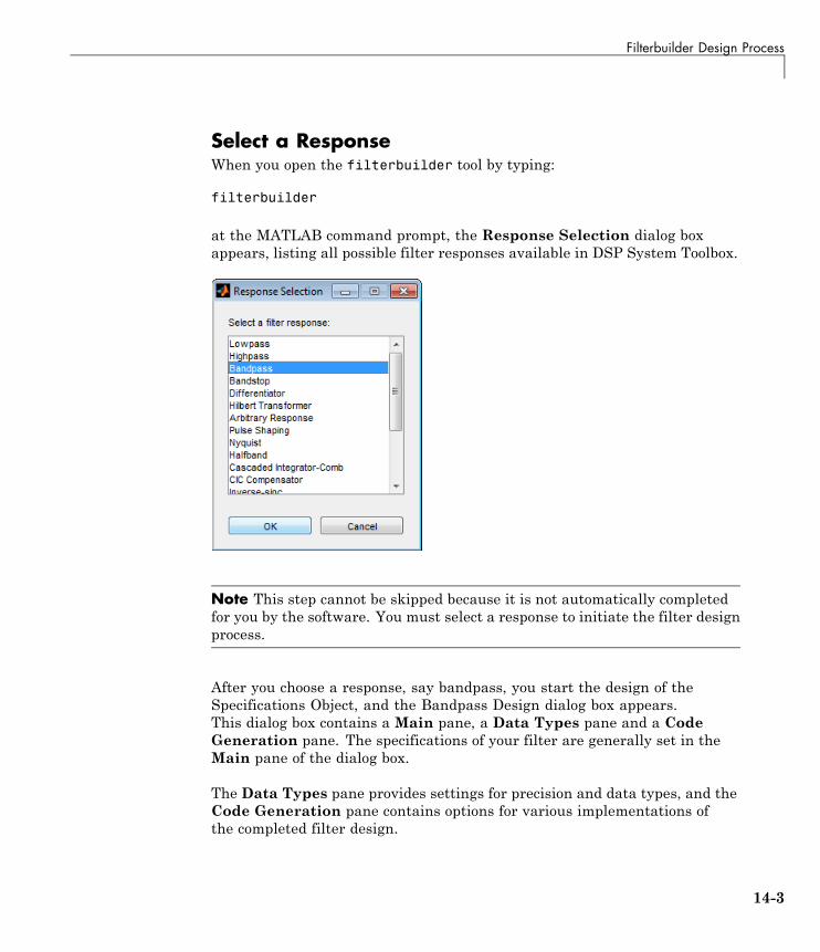
Filterbuilder Design Process
Select a ResponseWhen you open the filterbuilder tool by typing:
filterbuilder
at the MATLAB command prompt, the Response Selection dialog boxappears, listing all possible filter responses available in DSP System Toolbox.
Note This step cannot be skipped because it is not automatically completedfor you by the software. You must select a response to initiate the filter designprocess.
After you choose a response, say bandpass, you start the design of theSpecifications Object, and the Bandpass Design dialog box appears.This dialog box contains a Main pane, a Data Types pane and a CodeGeneration pane. The specifications of your filter are generally set in theMain pane of the dialog box.
The Data Types pane provides settings for precision and data types, and theCode Generation pane contains options for various implementations ofthe completed filter design.
14-3
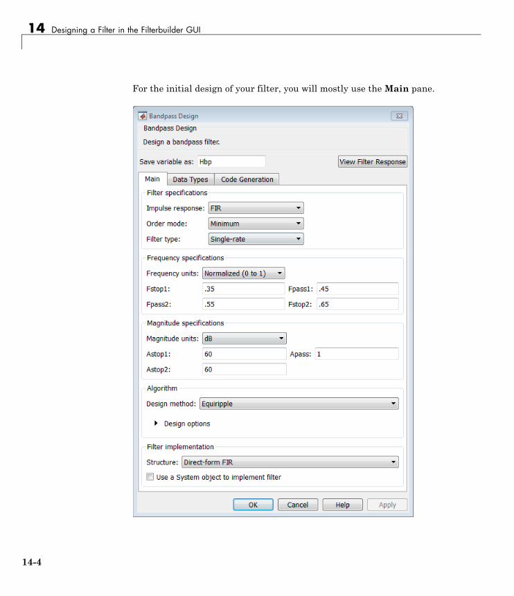
14 Designing a Filter in the Filterbuilder GUI
For the initial design of your filter, you will mostly use theMain pane.
14-4
Filterbuilder Design Process
The Bandpass Design dialog box contains all the parameters you need todetermine the specifications of a bandpass filter. The parameters listed inthe Main pane depend upon the type of filter you are designing. However,no matter what type of filter you have chosen in the Response Selectiondialog box, the filter design dialog box contains the Main, Data Types, andCode Generation panes.
Select a SpecificationTo choose the specification for the bandpass filter, you can begin by selectingan Impulse Response, Order Mode, and Filter Type in the FilterSpecifications frame of the Main Pane. You can further specify theresponse of your filter by setting frequency and magnitude specifications inthe appropriate frames on the Main Pane.
Note Frequency, Magnitude, and Algorithm specifications areinterdependent and may change based upon your Filter Specificationsselections. When choosing specifications for your filter, select your FilterSpecifications first and work your way down the dialog box- this approachensures that the best settings for dependent specifications display as availablein the dialog box.
Select an AlgorithmThe algorithms available for your filter depend upon the filter response anddesign parameters you have selected in the previous steps. For example, in thecase of a bandpass filter, if the impulse response selected is IIR and the OrderMode field is set to Minimum, the design methods available are Butterworth,Chebyshev type I or II, or Elliptic, whereas if the Order Mode field is setto Specify, the design method available is IIR least p-norm.
14-5

14 Designing a Filter in the Filterbuilder GUI
14-6

Filterbuilder Design Process
Customize the AlgorithmBy expanding the Design options section of the Algorithm frame, youcan further customize the algorithm specified. The options available willdepend upon the algorithm and settings that have already been selected inthe dialog box. In the case of a bandpass IIR filter using the Butterworthmethod, design options such as Match Exactly are available, as shown inthe following figure.
14-7
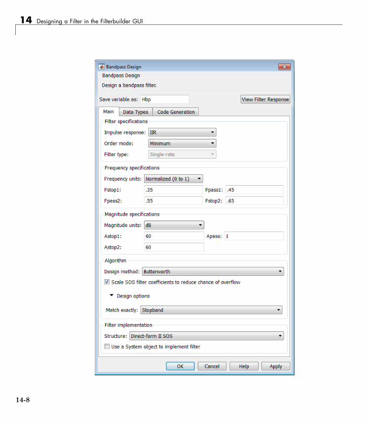
14 Designing a Filter in the Filterbuilder GUI
14-8

Filterbuilder Design Process
Analyze the DesignTo analyze the filter response, click on the View Filter Response button. TheFilter Visualization Tool opens displaying the magnitude plot of the filterresponse.
Realize or Apply the Filter to Input DataWhen you have achieved the desired filter response through design iterationsand analysis using the Filter Visualization Tool, apply the filter to theinput data. Again, this step is never automatically performed for you by thesoftware. To filter your data, you must explicitly execute this step. In theBandpass Design dialog box, click OK and DSP System Toolbox creates thefilter object and exports it to the MATLAB workspace.
The filter is then ready to be used to filter actual input data. The basic filtercommand takes input data x, filters it through the Filter Object, and producesoutput y:
>> y = filter (Hbp, x)
14-9

14 Designing a Filter in the Filterbuilder GUI
To understand how the filtering commands work, type:
>> help dfilt/filter
Tip If you have Simulink, you have the option of exporting this filter toa Simulink block using the realizemdl command. To get help on thiscommand, type:
>> help realizemdl
14-10

Designing a FIR Filter Using filterbuilder
Designing a FIR Filter Using filterbuilder
FIR Filter Design
Example – Using Filterbuilder to Design a Finite Impulse Response(FIR) FilterTo design a lowpass FIR filter using filterbuilder:
1 Open the Filterbuilder GUI by typing the following at the MATLAB prompt:
filterbuilder
The Response Selection dialog box appears. In this dialog box, you canselect from a list of filter response types. Select Lowpass in the list box.
2 Hit the OK button. The Lowpass Design dialog box opens. Here youcan specify the writable parameters of the Lowpass filter object. Thecomponents of the Main frame of this dialog box are described in thesection titled Lowpass Filter Design Dialog Box — Main Pane. In the dialogbox, make the following changes:
• Enter a Fpass value of 0.55.
• Enter a Fstop value of 0.65.
14-11
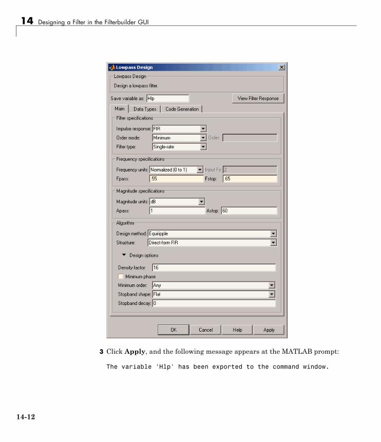
14 Designing a Filter in the Filterbuilder GUI
3 Click Apply, and the following message appears at the MATLAB prompt:
The variable 'Hlp' has been exported to the command window.
14-12
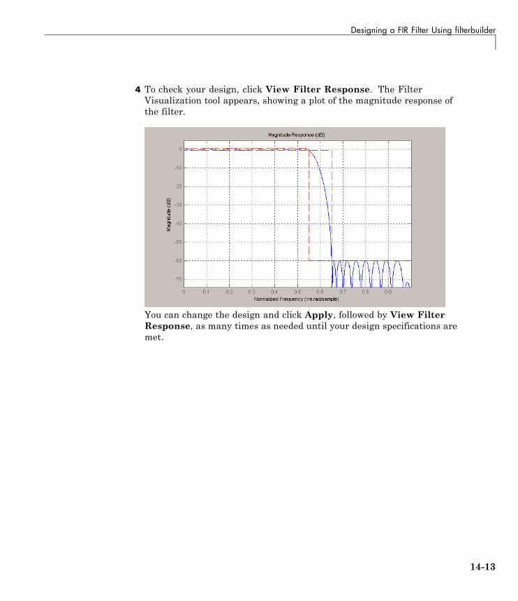
Designing a FIR Filter Using filterbuilder
4 To check your design, click View Filter Response. The FilterVisualization tool appears, showing a plot of the magnitude response ofthe filter.
You can change the design and click Apply, followed by View FilterResponse, as many times as needed until your design specifications aremet.
14-13

14 Designing a Filter in the Filterbuilder GUI
14-14

A
Bibliography
• “Advanced Filters” on page A-2
• “Adaptive Filters” on page A-3
• “Multirate Filters” on page A-4
• “Frequency Transformations” on page A-5
• “Fixed-Point Filters” on page A-6

A Bibliography
Advanced Filters[1] Antoniou, A., Digital Filters: Analysis, Design, and Applications, SecondEdition, McGraw-Hill, Inc., 1993.
[2] Chirlian, P.M., Signals and Filters, Van Nostrand Reinhold, 1994.
[3] Fliege, N.J., Multirate Digital Signal Processing, John Wiley and Sons,1994.
[4] Jackson, L., Digital Filtering and Signal Processing with MATLABExercises, Third edition, Springer, 1995.
[5] Lapsley, P., J. Bier, A. Sholam, and E.A. Lee, DSP ProcessorFundamentals: Architectures and Features, IEEE Press, 1997.
[6] McClellan, J.H., C.S. Burrus, A.V. Oppenheim, T.W. Parks, R.W. Schafer,and H.W. Schuessler, Computer-Based Exercises for Signal Processing UsingMATLAB 5, Prentice-Hall, 1998.
[7] Mayer-Baese, U., Digital Signal Processing with Field Programmable GateArrays, Springer, 2001, refer to the BiQuad block diagram on pp. 126 and theIIR Butterworth example on pp. 140.
[8] Moler, C., “Floating points: IEEE Standard unifies arithmeticmodel.” Cleve’s Corner, The MathWorks, Inc., 1996. Seehttp://www.mathworks.com/company/newsletter/pdf/Fall96Cleve.pdf.
[9] Oppenheim, A.V., and R.W. Schafer, Discrete-Time Signal Processing,Prentice-Hall, 1989.
[10] Shajaan, M., and J. Sorensen, “Time-Area Efficient Multiplier-FreeRecursive Filter Architectures for FPGA Implementation,” IEEE InternationalConference on Acoustics, Speech, and Signal Processing, 1996, pp. 3269-3272.
A-2

Adaptive Filters
Adaptive Filters[1] Hayes, M.H., Statistical Digital Signal Processing and Modeling, JohnWiley and Sons, 1996.
[2] Haykin, S., Adaptive Filter Theory, Third Edition, Prentice-Hall, Inc.,1996.
A-3
A Bibliography
Multirate Filters[1] Fliege, N.J., Multirate Digital Signal Processing, John Wiley and Sons,1994.
[2] Harris, Fredric J, Multirate Signal Processing for CommunicationSystems, Prentice Hall PTR, 2004.
[3] Hogenauer, E. B., “An Economical Class of Digital Filters for Decimationand Interpolation,” IEEE Transactions on Acoustics, Speech, and SignalProcessing, Vol. ASSP-29, No. 2, April 1981, pp. 155-162.
[4] Lyons, Richard G., Understanding Digital Signal Processing, PrenticeHall PTR, 2004
[5] Mitra, S.K., Digital Signal Processing, McGraw-Hill, 1998.
[6] Orfanidis, S.J., Introduction to Signal Processing, Prentice-Hall, Inc.,1996.
A-4
Frequency Transformations
Frequency Transformations[1] Constantinides, A.G., “Spectral Transformations for Digital Filters,” IEEEProceedings, Vol. 117, No. 8, pp. 1585-1590, August 1970.
[2] Nowrouzian, B., and A.G. Constantinides, “Prototype Reference TransferFunction Parameters in the Discrete-Time Frequency Transformations,”Proceedings 33rd Midwest Symposium on Circuits and Systems, Calgary,Canada, Vol. 2, pp. 1078-1082, August 1990.
[3] Feyh, G., J.C. Franchitti, and C.T. Mullis, “Allpass Filter Interpolationand Frequency Transformation Problem,“ Proceedings 20th AsilomarConference on Signals, Systems and Computers, Pacific Grove, California,pp. 164-168, November 1986.
[4] Krukowski, A., G.D. Cain, and I. Kale, “Custom Designed High-OrderFrequency Transformations for IIR Filters,” 38th Midwest Symposium onCircuits and Systems (MWSCAS’95), Rio de Janeiro, Brazil, August 1995.
A-5
A Bibliography
Fixed-Point Filters[1] Jackson, L., Digital Filtering and Signal Processing with MATLABExercises, Third edition, Springer, 1995, pp.373–422.
[2] Dehner, G, “Noise optimized IIR digital filter design: tutorial and somenew aspects,” Signal Processing, Vol 83, Issue 8 (August 2003) pp.1565–1582.
A-6