dscp: depthwise separable convolution-based passive indoor

Research ArticleDSCP: Depthwise Separable Convolution-Based Passive IndoorLocalization Using CSI Fingerprint

Chong Han ,1,2 Wenjing Xun,1 Lijuan Sun,1,2 Zhaoxiao Lin,1 and Jian Guo1,2

1College of Computer, Nanjing University of Posts and Telecommunications, Nanjing 210003, China2Jiangsu High Technology Research Key Laboratory for Wireless Sensor Networks, Nanjing University of Postsand Telecommunications, Nanjing 210003, China

Correspondence should be addressed to Chong Han; [email protected]

Received 12 August 2020; Revised 7 December 2020; Accepted 22 December 2020; Published 4 January 2021

Academic Editor: Miguel Garcia-Pineda

Copyright © 2021 Chong Han et al. This is an open access article distributed under the Creative Commons Attribution License,which permits unrestricted use, distribution, and reproduction in any medium, provided the original work is properly cited.

Wi-Fi-based indoor localization has received extensive attention in wireless sensing. However, most Wi-Fi-based indoorlocalization systems have complex models and high localization delays, which limit the universality of these localizationmethods. To solve these problems, a depthwise separable convolution-based passive indoor localization system (DSCP) isproposed. DSCP is a lightweight fingerprint-based localization system that includes an offline training phase and an onlinelocalization phase. In the offline training phase, the indoor scenario is first divided into different areas to set training locationsfor collecting CSI. Then, the amplitude differences of these CSI subcarriers are extracted to construct location fingerprints,thereby training the convolutional neural network (CNN). In the online localization phase, CSI data are first collected at the testlocations, and then, the location fingerprint is extracted and finally fed to the trained network to obtain the predicted location.The experimental results show that DSCP has a short training time and a low localization delay. DSCP achieves a highlocalization accuracy, above 97%, and a small median localization distance error of 0.69m in typical indoor scenarios.

1. Introduction

1.1. Background. As mobile smart devices and wireless net-works influence all aspects of human production and life,location-based services (LBSs) have gradually become indis-pensable in people’s lives [1]. Although global positioningsystems (GPSs) have become a leader in outdoor navigationand localization, the severe decline in GPS signals causedby reinforced concrete makes it difficult to navigate andlocalize indoors. The great research significance and practicalvalue of indoor localization have attracted a large number ofresearchers, with a large number of indoor localization [2–4]methods emerging. Currently, wireless sensor networks,computer vision, ultrasonic, ultrawideband, Bluetooth, andRFID [5, 6] are mainly used in indoor localization. However,most of these localization methods require a large number ofhardware devices, which limits the universality of localiza-tion. With the widespread adoption of Wi-Fi, an increasingnumber of researchers have applied Wi-Fi to wireless sens-

ing. Wi-Fi-based indoor localization methods [7–9] havegradually become mainstream.

The received signal strength (RSS), as the main energycharacteristic measurement of wireless signals, can bedirectly obtained from most wireless terminals and is widelyused in Wi-Fi-based indoor localization systems [10].RADAR, proposed by Microsoft Research, was the first sys-tem to implement indoor localization using WLAN [11].RADAR uses RSS and fingerprint matching and proposed afingerprint-based localization method for the first time.However, in the indoor environment, wireless signals propa-gate from the transmitter to the receiver through multiplepaths due to the presence of obstacles such as walls and fur-niture. The signals received by the receiver are the superposi-tion of signals from multiple paths. As an average ofmultipath signals, the RSS is unstable in indoor environ-ments, which limits the reliability and localization accuracyof RSS-based indoor localization systems. Compared toRSS, channel state information (CSI) is fine-grained

HindawiWireless Communications and Mobile ComputingVolume 2021, Article ID 8821129, 17 pageshttps://doi.org/10.1155/2021/8821129

https://orcid.org/0000-0002-2657-1464

https://creativecommons.org/licenses/by/4.0/

https://creativecommons.org/licenses/by/4.0/

https://doi.org/10.1155/2021/8821129

information from the PHY layer, which describes multipathpropagation. Figuratively speaking, CSI is to RSS what a rain-bow is to a sunbeam [12]. By modifying the firmware, a sam-ple version of the channel frequency response (CFR) can beobtained in the form of CSI from some Wi-Fi network inter-face cards (NICs), such as Intel 5300. Each set of CSIs char-acterizes the amplitude and phase of orthogonal frequencydivision multiplexing (OFDM) subcarriers. Therefore, CSIhas better static stability and dynamic sensitivity [13]. Manyresearchers have begun to use CSI in indoor localization [14–16].

Fingerprints of different locations are generally different.Therefore, many researchers use classification algorithms toimplement fingerprint-based localization. As traditional clas-sification algorithms, kNN and Bayesian classification arewidely used in fingerprint-based localization. There are manyfingerprint-based localizations in Wi-Fi wireless sensing. Senet al. proposed a fingerprint-based localization system calledPinLoc [17] using the distinguishability of CSI at differentlocations. Xiao et al. used the frequency diversity and spatialdiversity of CSI to construct subchannel power informationlocation fingerprints based on CSI amplitude and proposedthe FIFS system [18]. Xiao et al. subsequently proposed thefirst CSI-based passive indoor localization system Pilot [19].Pilot uses probability estimation to match the obtained CSIwith the fingerprint database to achieve position. Chapreet al. used the amplitude differences and phase differencesof CSI to construct fingerprints and proposed a Wi-Fi finger-print system CSI-MIMO [20]. Abdel-Nasser et al. [21]observed that the CSI probability density distribution of dif-ferent locations nicely fits a Gaussian distribution mixtureand used k-means to construct a cluster-based fingerprintdatabase. To improve the localization accuracy, Sabek et al.

propose a single access point-monitoring point- (AP-MP-)based localization system MonoStream [22], which modelsthe passive localization as an object recognition problem.

Compared with traditional methods, deep learning-basedmethods are more accurate. Wang et al. proposed deeplearning-based CSI fingerprint indoor localization systemsDeepFi and PhaseFi [23, 24] using the amplitude and phaseof CSI, respectively. In the offline training phase, the systemuses the weights of the deep learning training as the locationfingerprints. In the online localization phase, the probabilitymethod based on the radial basis function is used to obtainthe estimated location. Chen et al. proposed the first CNN-based Wi-Fi indoor localization system ConFi [25]. Whenextracting CSI features, ConFi simulates RGB images, whichhave three channels. The data of different transmitting-receiving antenna pairs in a multiple input multiple output(MIMO) system are regarded as the different channels ofthe image. ConFi predicts the location of the target by calcu-lating the probability of the target at different training points.Similarly, Cai et al. constructed location fingerprints basedon the amplitude of CSI and proposed a passive localizationsystem PILC [26].

Most CSI fingerprint localization systems based on tradi-tional methods have shortcomings, such as the single featuresof location fingerprint information and complex models.Although deep learning methods can mine more features,the training of network models generally takes considerabletime and limits the real-time capability of localization. There-fore, we propose a CSI fingerprint localization system basedon a lightweight convolutional neural network.

1.2. Our Contributions. In our method, we extract amplitudesof CSI subcarriers from data of different transmitting-

Table 1: CSI grouping of 20MHz bandwidth in 802.11n.

BW Grouping Ng Ns Carriers for which matrices are sent

20MHz

1 56 All carriers: -28, -27, ... -2, -1, 1, 2, ...,27, 28

2 30 -28, -26, -24, -22, -20, -18, -16, -14, -12, -10, -8, -6, -4, -2, -1, 1, 3, 5, 7, 9, 11, 13, 15, 17, 19, 21, 23, 25, 27, 28

4 16 -28, -24, -20, -16, -12, -8, -4, -1, 1, 5, 9, 13, 17, 21, 5, 28

N

M

K

K

(a) Standard convolution filters

MK

K

1

(b) Depthwise convolution filters

N

M

11

(c) 1 × 1 convolutional filters called pointwise convolution in the context of depthwise separable convolution

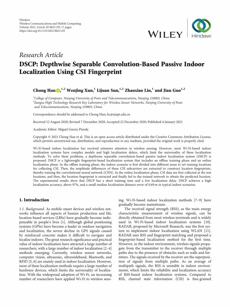
Figure 1: Depthwise separable convolution [30].

2 Wireless Communications and Mobile Computing

receiving antenna pairs and calculate the differences. Then,we use amplitude differences to construct CSI feature images.Each channel of the CSI feature image corresponds to data ofone transmitting-receiving antenna pair. We design a depth-wise separable convolution-based network consisting ofseven convolutional layers. In the offline training phase, wecollect CSI indoors and construct CSI feature images for net-work training. In the online localization phase, CSI featureimages of test data are sent to the trained network to obtainthe predicted location.

The main contributions of this paper are as follows:

(i) This paper proposes to use depthwise separable con-volutions in the network to speed up network train-ing and reduce localization delay in an indoorlocalization system based on a CSI fingerprint

(ii) The proposed indoor localization system uses CSIfeature images constructed from the amplitude dif-ference of CSI subcarriers as location fingerprints.Similar to CSI feature images based on the amplitudeof subcarriers, CSI feature images based on theamplitude difference of subcarriers combine time,frequency, and spatial domain information

(iii) The proposed indoor localization system uses CSIfeature images based on the amplitude difference ofsubcarriers, which can reflect the difference in thesignal attenuation of different subcarriers in multiple

paths and amplify the differences between differentlocation fingerprints

The remainder of this paper is organized as follows. Therelated work and the preliminary are presented in Section 2.The DSCP system is presented in Section 3. Section 4 pro-vides the experimental validation, while Section 5 concludesthe paper.

2. Preliminary

This section introduces the concepts needed for the subse-quent analysis, including CSI background information,

Offline phase(Training phase)

Offline phase(Localization phase)

Train CSI data Train CSI data

CSI amplitudedifference

CSI amplitudedifference

CSI feature images CSI feature images

Locationestimation

DCCPnetwork

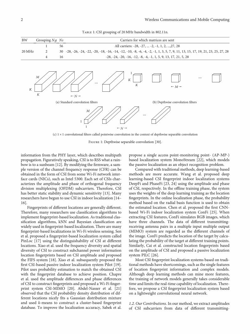
Figure 2: DSCP architecture.

30

30 30 30 30

3030 30

3 64 64 256256

15

15 15

158

88

811

1024 1024 1024 1024

32FCPool: 8 8

stride: 1Pointwise

convolutions:1 1

stride: 1

Pointwiseconvolutions:

1 1stride: 1

Pointwiseconvolutions:

1 1stride: 1

Deathwiseconvolutions:

3 3stride: 2


3 3stride: 2


3 3stride: 1

Convolutions:3 3

stride: 1

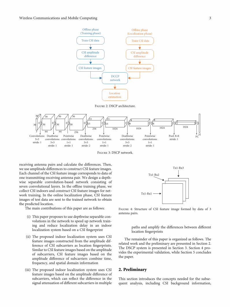
Figure 3: DSCP network.

Tx1-Rx2

Tx1-Rx1

Tx1-Rx3

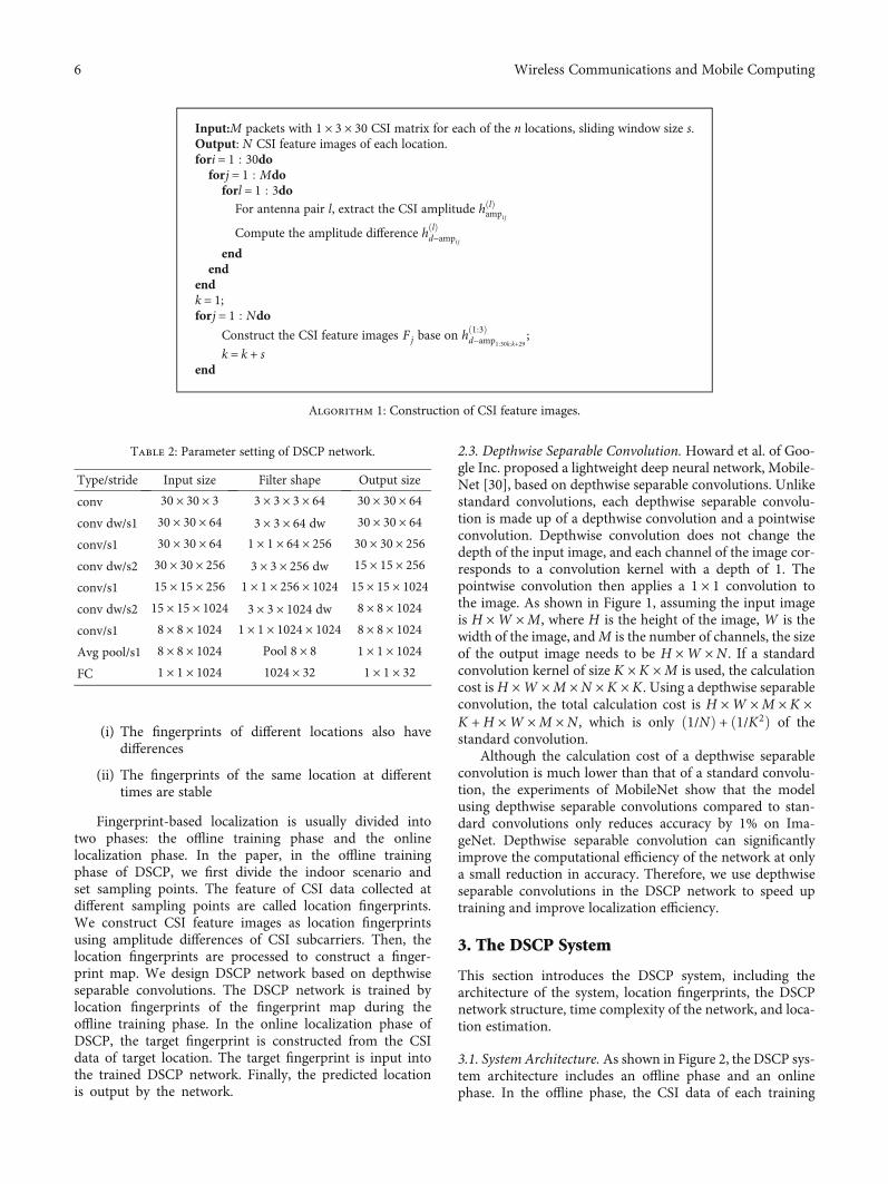
Figure 4: Structure of CSI feature image formed by data of 3antenna pairs.

3Wireless Communications and Mobile Computing

fingerprint-based localization, and depthwise separableconvolution.

2.1. Channel State Information. CSI represents the channelcharacteristics of the communication link between the trans-mitter and the receiver, reflecting the effects of scattering,attenuation, etc. of the signal propagation. According to IEEE802.11n [27], a signal can be transmitted through a set of sub-carriers with different frequencies and mutually orthogonalby OFDM. To estimate the CSI matrix, the transmitter trans-mits a known pilot sequence x1, x2,⋯, xn, and the combinedreceived signal Y can be expressed as

Y = y1, y2,⋯, yn½ � =HX +N , ð1Þ

where H is the CSI matrix and N is the noise.

Therefore, the CSI matrix can be approximated as

H = YX: ð2Þ

For a system with N subcarriers, H can be expressed as

H = H1,H2,⋯,HN½ �, ð3Þ

where

Hi = Hij jej sin ∠Hið Þ: ð4Þ

For a MIMO system withm transmitting antennas and n

5

5

10

10

15

15

20

20

25

2530

30

(a) CSI fingerprint of location 1

5

5

10

10

15

15

20

20

25

25

30

30

(b) CSI fingerprint of location 2

Figure 5: CSI feature images based on subcarrier amplitudes.


receiving antennas, Hi can be expressed as

Hi =

h11 h12

h21 h22

⋯ h1n

⋯ h2n

⋮ ⋮

hm1 hm2

⋱ ⋮

⋯ hmn

26666666666664

37777777777775, ð5Þ

where hpqðp ∈ ½1,m�, q ∈ ½1, n�Þ corresponds to the complexnumber of subcarrier amplitudes and phases on the stream.

There are 56 subcarries in total in the 20 bandwidth and114 subcarries in the 40 bandwidth. Grouping is a method

that reduces the size of the CSI Report field by reporting asingle value for each group of Ng adjacent subcarriers [27].The subcarrier frequency spacing is 312.5 in the 20 channel[28]. As shown in Table 1, for a 20 bandwidth, there are threegrouping modes defined in IEEE 802.11n. Ns is the numberof subcarriers sent. This paper is based on the Wi-Fi CSI ina 20 channel.

2.2. Fingerprint-Based Localization. In an indoor environ-ment, due to walls and obstacles, wireless signals form multi-path effects. Humans at different physical locations havedifferent effects on wireless signal propagation paths. The dif-ferences can be expressed as fingerprints that reflect the char-acteristics of humans at different locations [29]. Generally, inthe case of small indoor environment changes, a valid loca-tion fingerprint needs to meet the following two conditions:

5

5

10

10

15

15

20

20

25

2530

30

(a) CSI fingerprint of location 1

5

5

10

10

15

15

20

20

25

2530

30

(b) CSI fingerprint of location 2

Figure 6: CSI feature images based on subcarrier amplitudes differences.


(i) The fingerprints of different locations also havedifferences

(ii) The fingerprints of the same location at differenttimes are stable

Fingerprint-based localization is usually divided intotwo phases: the offline training phase and the onlinelocalization phase. In the paper, in the offline trainingphase of DSCP, we first divide the indoor scenario andset sampling points. The feature of CSI data collected atdifferent sampling points are called location fingerprints.We construct CSI feature images as location fingerprintsusing amplitude differences of CSI subcarriers. Then, thelocation fingerprints are processed to construct a finger-print map. We design DSCP network based on depthwiseseparable convolutions. The DSCP network is trained bylocation fingerprints of the fingerprint map during theoffline training phase. In the online localization phase ofDSCP, the target fingerprint is constructed from the CSIdata of target location. The target fingerprint is input intothe trained DSCP network. Finally, the predicted locationis output by the network.

2.3. Depthwise Separable Convolution. Howard et al. of Goo-gle Inc. proposed a lightweight deep neural network, Mobile-Net [30], based on depthwise separable convolutions. Unlikestandard convolutions, each depthwise separable convolu-tion is made up of a depthwise convolution and a pointwiseconvolution. Depthwise convolution does not change thedepth of the input image, and each channel of the image cor-responds to a convolution kernel with a depth of 1. Thepointwise convolution then applies a 1 × 1 convolution tothe image. As shown in Figure 1, assuming the input imageis H ×W ×M, where H is the height of the image, W is thewidth of the image, andM is the number of channels, the sizeof the output image needs to be H ×W ×N . If a standardconvolution kernel of size K × K ×M is used, the calculationcost isH ×W ×M ×N × K × K . Using a depthwise separableconvolution, the total calculation cost is H ×W ×M × K ×K +H ×W ×M ×N , which is only ð1/NÞ + ð1/K2Þ of thestandard convolution.

Although the calculation cost of a depthwise separableconvolution is much lower than that of a standard convolu-tion, the experiments of MobileNet show that the modelusing depthwise separable convolutions compared to stan-dard convolutions only reduces accuracy by 1% on Ima-geNet. Depthwise separable convolution can significantlyimprove the computational efficiency of the network at onlya small reduction in accuracy. Therefore, we use depthwiseseparable convolutions in the DSCP network to speed uptraining and improve localization efficiency.

3. The DSCP System

This section introduces the DSCP system, including thearchitecture of the system, location fingerprints, the DSCPnetwork structure, time complexity of the network, and loca-tion estimation.

3.1. System Architecture. As shown in Figure 2, the DSCP sys-tem architecture includes an offline phase and an onlinephase. In the offline phase, the CSI data of each training

Input:M packets with 1 × 3 × 30 CSI matrix for each of the n locations, sliding window size s.Output: N CSI feature images of each location.fori = 1 : 30do

forj = 1 : Mdoforl = 1 : 3do

For antenna pair l, extract the CSI amplitude hðlÞampi j

Compute the amplitude difference hðlÞd−ampi jend

endendk = 1;forj = 1 : Ndo

Construct the CSI feature images Fj base on hð1:3Þd−amp1:30k:k+29 ;

k = k + send

Algorithm 1: Construction of CSI feature images.

Table 2: Parameter setting of DSCP network.

Type/stride Input size Filter shape Output size

conv 30 × 30 × 3 3 × 3 × 3 × 64 30 × 30 × 64conv dw/s1 30 × 30 × 64 3 × 3 × 64 dw 30 × 30 × 64conv/s1 30 × 30 × 64 1 × 1 × 64 × 256 30 × 30 × 256conv dw/s2 30 × 30 × 256 3 × 3 × 256 dw 15 × 15 × 256conv/s1 15 × 15 × 256 1 × 1 × 256 × 1024 15 × 15 × 1024conv dw/s2 15 × 15 × 1024 3 × 3 × 1024 dw 8 × 8 × 1024conv/s1 8 × 8 × 1024 1 × 1 × 1024 × 1024 8 × 8 × 1024Avg pool/s1 8 × 8 × 1024 Pool 8 × 8 1 × 1 × 1024FC 1 × 1 × 1024 1024 × 32 1 × 1 × 32


location are first collected, and then, the amplitude of the CSIis extracted. DSCP constructs CSI feature images as finger-prints of each training location for training the network. Inthe online phase, the CSI data of the target location are col-lected, and the fingerprint of the target location is extractedto be input into the trained network. Finally, the predictedlocation is output by the DSCP network. The DSCP networkhas seven convolutional layers, as shown in Figure 3.

3.2. Location Fingerprint. Thirty subcarriers can be read forCSI information via Intel 5300 NIC. In this paper, we usethe subcarrier amplitudes when constructing the location fin-gerprints. Each packet contains a 1 × 3 × 30 CSI matrix,which corresponds to the complex numbers of subcarrieramplitudes and phases on the stream. For eachtransmitting-receiving antenna pair, a sliding window of sizeM is used to selectM consecutive data packets in a sequence.To match the 30 subcarriers, we make the height and widthof CSI feature images the same. So we set M to 30, whichmeans subcarriers of 30 consecutive data packets are chosento construct one 30 × 30 matric. Multiple sets of 30 × 30matrices are constructed. The structure of CSI feature imagesis shown in Figure 4. Similar to RGB images, the data of eachantenna pair correspond to one channel, and each locationhas some CSI feature images of 30 × 30 × 3 [25]. As shownin Figure 5, the CSI feature images formed by the amplitudesof subcarriers can reflect the difference of adjacent locations.

The amplitudes of the subcarriers characterize the powerfading of the wireless signals between the transmitter and

receiver [31]. The signal received by the receiver also containsmeasurement noise. The frequency difference between adja-cent subcarriers is 625 kHz in our experiments. Different fre-quency subcarriers are affected differently by the multipatheffect, and the difference can be reflected in the subcarrieramplitude. ConFi [25] is the first CNN-based Wi-Fi indoorlocalization system, which proposes to use CSI feature imagesas location fingerprints. ConFi uses amplitudes of subcarriersfrom consecutive data packets to construct CSI featureimages. ConFi maps the CSI feature subimages from the dif-ferent antenna pairs into the RGB channels of the image. Theelements in the row are amplitudes of 30 subcarriers in onepacket. The experiments of ConFi show that CSI featureimage of size 30 × 30 gets the highest accuracy, which isabout 90% on test set. Therefore, CSI feature images basedon amplitude of CSI subcarriers are valid location finger-prints. In indoor environments, wireless signals are affectedby multipath effects. We consider that the amplitudes of thesubcarriers are greatly affected by the physical environment,which may result in little influence of humans on CSI. Differ-ent from ConFi, to amplify the differences between finger-prints of different locations, we use the amplitudedifferences between adjacent subcarriers to construct CSI fea-ture images at different locations. The CSI feature imagescombine the time domain, frequency domain, and spatialdomain information of CSI data. Therefore, the CSI featureimages of each location are used as the location fingerprints(as shown in Figure 6).

For transmitting antenna p and receiving antenna q, theamplitude of subcarrier i in packet j can be expressed as

hampi j = hpq��

ij: ð6Þ

The amplitude difference between adjacent subcarriers is

hd−ampij=

hampi+1 j− hampij

i ∈ 1, 29½ �ð Þ,hamp1 j

− hampiji = 30ð Þ:

8>><>>: ð7Þ

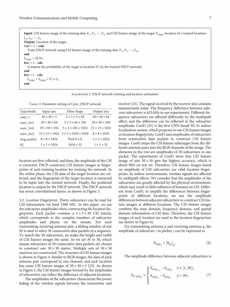
Input: CSI feature image of the training data F1, F2,⋯, Fm and CSI feature image of the target Ftarget, location of n trained locationsL1, L2,⋯, LnOutput: Location of the target.Fori = 1 : mdo

Train DSCP network using CSI feature image of the training data F1, F2,⋯, Fm;endLtarget = ð0, 0Þ;fori = 1 : ndo

Compute the probability of the target at location iPi by the trained DSCP network;endfori = 1 : ndo

Ltarget = Ltarget + Pi × Li;end

Algorithm 2: DSCP network training and location estimation.

Table 3: Parameter setting of Conv_DSCP network.

Type/stride Input size Filter shape Output size

conv_1 30 × 30 × 3 3 × 3 × 3 × 64 30 × 30 × 64conv_2/s1 30 × 30 × 64 3 × 3 × 64 × 256 30 × 30 × 256conv_3/s2 30 × 30 × 256 3 × 3 × 256 × 1024 15 × 15 × 1024conv_4/s2 15 × 15 × 1024 3 × 3 × 1024 × 1024 8 × 8 × 1024Avg pool/s1 8 × 8 × 1024 Pool 8 × 8 1 × 1 × 1024FC 1 × 1 × 1024 1024 × 32 1 × 1 × 32


Then, a CSI feature image can be expressed as

F =

hd−amp1k hd−amp2k ⋯ hd−ampNk

hd−amp1k+1 hd−amp2k+1 ⋯ hd−ampNk+1

⋮ ⋮ ⋱ ⋮

hd−amp1k+29 hd−amp2k+29 ⋯ hd−ampNk+29

2666666664

3777777775: ð8Þ

The pseudocode for CSI feature image construction ispresented in Algorithm 1. The input of the algorithm

includes M packets with 1 × 3 × 30 CSI matrix for each ofthe n locations and sliding window size s. First, for data ofeach transmitting-receiving antenna pair, we extract theamplitude of CSI subcarriers from each packet (line 4). Then,we compute the amplitude difference (line 5). Finally, we usea sliding window to group the amplitude difference of 30packets to construct n CSI feature images of each location(lines 10-13).

3.3. Network Structure. Inspired by MobileNet, we design theDSCP network. The DSCP network is based on depthwiseseparable convolutions, which have seven convolutional

Figure 7: Scenario 1 is a laboratory.

Figure 8: Scenario 2 is a laboratory. Figure 9: Scenario 3 is an office.


layers. The first convolutional layer of the DSCP network is afull convolution, and the others are depthwise separable con-volutions. Table 2 shows the network structure. In the net-work, the standard convolution, pointwise convolutions,and first depthwise convolution stride are set to 1 to keepthe size of the image. The second and third depthwise convo-lution strides are set to 2. There is a batchnorm and ReLUafter each depthwise convolution and pointwise convolution.Since only 30 subcarriers can be extracted with the Intel 5300NIC, the sizes of the CSI feature images are much smallerthan real images. Therefore, the size of each DSCP depthwiseconvolution is set to 3 × 3. The output size of the final fullyconnected layer depends on the number of training locations.Adam [32] is an effective random optimization algorithmwith high computational efficiency and low memory require-ments. We use Adam optimization in the network training.

Similar to processing images with the CNN, DSCP con-siders the amplitude differences between four adjacent sub-carriers of the same packet in each convolution. Moreover,for the same pair of adjacent subcarriers, DSCP also con-siders their amplitude differences at three consecutive timepoints. Therefore, the DSCP network can learn the correla-tion of the CSI amplitude differences in the time and fre-quency domains.

Three channels of the CSI feature images correspond tothe data of different transmitting-receiving antenna pairs inthe MIMO system. The standard convolution considers dif-ferent channels of the image simultaneously in the convolu-tion. Different from standard convolutions, the depthwiseconvolutions of DSCP use different convolution kernels forthree channels of the CSI feature images separately. DSCPrealizes the complete separation of learning the frequencydomain, time domain correlation, and learning spatialdomain correlation of the CSI subcarriers, reducing the cou-pling of the convolution kernels.

3.4. Location Estimation. During the localization phase, testdata will be fed to the trained network, which will outputthe probability of the test data at each of the trained locations.Probability-based methods tend to have higher precisionthan classification-based methods. Therefore, we use theweighted mean method based on probability to estimate thefinal location. Assuming that there are N training locations,the coordinate of the ith training location is Li, and the prob-ability of the test data at the ith training location is Pi, theestimated location can be expressed as

L = 〠N

i=1‍Pi × Li: ð9Þ

The pseudocode for network training and location esti-mation is presented in Algorithm 2. The input of the algo-rithm are the CSI feature images for training and CSIfeature image of the target. First, CSI feature images are usedto train the DSCP network (lines 1-3). Then, the probabilityof the target at each training location will be computed bysending the CSI feature image of the target to the trainedDSCP network (line 6). Then, we use the method of weightedmeanmethod based on probability to estimate the location ofthe target (lines 8-10).

3.5. Time Complexity of the Network. The total time complex-ity of all convolutional layers [33] is

O 〠d

l=1‍nl−1 · s2l · nl ·m2

l

!, ð10Þ

where l is the index of a convolutional layer, d is thenumber of convolutional layers, nl is the output channelsof the lth layer, ml is the length of the output feature

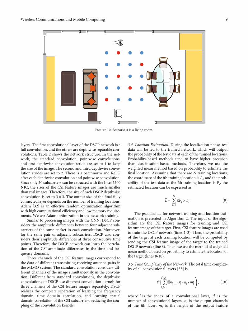
Figure 10: Scenario 4 is a living room.


image, and sl is the length of the filter. The time com-plexity of the network is the sum of the time complexityof each layer.

If only using standard convolution kernels, the DSCPnetwork will have 4 convolutional layers, and the structureis shown in Table 3. We estimate the time complexity ofthe DSCP and Conv_DSCP networks. For simplicity, we onlyconsider the convolutional layers. Assume the size of theinput image is S × S, and the calculation cost of Conv_DSCPis approximately 4,867,776 S2. The DSCP is approximately163,397.5 S2, which is only 3.36% of the Conv_DSCP. Thus,the DSCP can achieve a short low network training timeand low localization delay.

4. Experiment Validation

To illustrate the performance of the proposed DSCP method,a set of comparisons are performed with the other three

0 100 200 300 400 500 600 700 800 900 1000

Epoch

0

0.5

1

1.5

2

2.5

3

3.5

4

4.5

Trai

ning

loss

PILCConFiDSCP

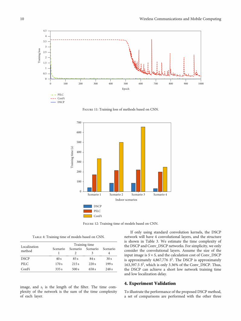
Figure 11: Training loss of methods based on CNN.

Scenario 1 Scenario 2 Scenario 3 Scenario 4Indoor scenarios

0

100

200

300

400

500

600

700

Trai

ning

tim

e (s)

DSCPPILCConFi

Figure 12: Training time of models based on CNN.

Table 4: Training time of models based on CNN.

Localizationmethod

Training timeScenario

1Scenario

2Scenario

3Scenario

4

DSCP 40 s 85 s 84 s 30 s

PILC 170 s 215 s 220 s 199 s

ConFi 335 s 500 s 658 s 248 s


methods, including the two methods ConFi [25] and PILC[26] based on CNN and the other method DeepFi [23] basedon deep learning. The comparison analysis is based on thesame illustrative examples.

4.1. Experiments Setup. In the experiments, we use a TP-LINK router as the transmitter. A Dell commercial desktopPC equipped with Intel 5300 NIC and Ubuntu 14.04 is usedas the receiver. The TensorFlow is accelerated with aNIVIDA RTX2080 graphics card during the experiments.The sampling rate is set to 50Hz. DSCP is a single-targetlocalization system. When collecting data, there is only oneperson in the room.We wrote a script to perform data collec-tion. The tester stands at each location for 60 seconds, andthe receiver can automatically collect 3,000 data packets.The Intel 5300 NIC has three antennas, and the wirelessrouter has one antenna, which is just a 1 × 3 MIMO system.The amplitudes and phases of the 30 subcarriers can beacquired from the NIC. Due to the hardware, there are errorsin the phase information acquired by the common commer-cial network card, and the original phase information is oftennot directly used. It is common to calculate the exact phaseshift by means of multiple linear regression and then experi-

ment with the phase shift. To simplify the system, we onlyuse the amplitude information of CSI.

In this paper, four indoor scenarios were selected forexperiments (as shown in Figures 7–10). The samplingpoints were divided into training locations and test locationsmarked as blue and red, respectively. Scenario 1 was a 5:8m × 8:6m laboratory. A total of 32 sampling points wereset. The spacing between adjacent sampling points was 1m.Twenty-four locations were selected for training and 8 fortesting. Scenario 2 was a 40m2 laboratory. Forty-five loca-tions were selected for training, and 32 locations wereselected for testing. Scenario 3 was an office of 7:5m × 6:5m. Sixty-six locations were selected for training and 30 fortesting. The spacing between adjacent sampling points was0.6m in both Scenarios 2 and 3. Scenario 4 was a typical liv-ing room of 4m × 8m. Fifteen locations are selected fortraining and 5 for testing. The spacing between adjacent sam-pling points was 0.5m.

4.2. The Comparison Works. The performance of DSCP wasevaluated in four scenarios. We compared DSCP with threedeep learning-based methods, PILC [26], ConFi [25], andDeepFi [23]. ConFi was the first CNN-based Wi-Fi indoorlocalization system. PILC and ConFi both use CSI ampli-tudes to construct CSI feature images, which have threechannels. The data of different transmitting-receivingantenna pairs are used in a MIMO system. PILC is a passivelocalization system based on CNN. The PILC network has sixlayers. DeepFi uses CSI information for all the subcarriersfrom three antennas and proposes to use the weights in thedeep network to represent fingerprints. DeepFi uses a proba-bilistic data fusion method based on the radial basis foronline location estimation.

For DSCP, experiments based on CSI amplitude andamplitude differences were performed. The median distance

Scenario 1 Scenario 2 Scenario 3 Scenario 4

Indoor scenarios

0

0.1

0.2

0.3

0.4

0.5

0.6

0.7

0.8

0.9

1

Acc

urac

y

DSCP

PILC

ConFi

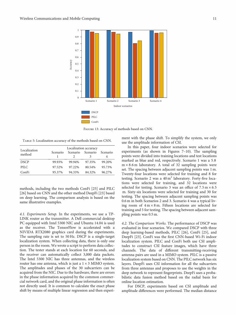
Figure 13: Accuracy of methods based on CNN.

Table 5: Localization accuracy of the methods based on CNN.

Localizationmethod

Localization accuracyScenario

1Scenario

2Scenario

3Scenario

4

DSCP 99.93% 99.94% 97.35% 99.20%

PILC 97.52% 97.22% 80.54% 95.73%

ConFi 95.37% 94.33% 84.32% 96.27%


error and the mean distance error of different localizationmethods were calculated. The median distance error wasthe median of all the test case localization errors. The meandistance error is the average of all the test case localizationerrors.

4.3. Model Evaluation. DSCP was compared with two CNN-based indoor localization methods, PILC and ConFi. Asshown in Figure 11, the training loss of PILC started to con-verge when the number of epochs was approximately 50. Thetraining loss of ConFi converged when the number of epochswas approximately 1,000. The training loss of the DSCP con-verged when the number of epochs is approximately 20. Insubsequent experiments, the values of the epoch were setaccording to convergence conditions of different networks.The network training time of the three localization methodsbased on the CNN is shown in Figure 12 and Table 4. Thetime unit is second.

In this experiment, 75% of all training location data werethe training set, and the remaining 25% were the test set. Thelocalization accuracies of DSCP, PILC, and ConFi were cal-culated. The batch sizes of DSCP and PILC were the numbersof training locations. The epochs of DSCP, PILC, and ConFiwere 30, 60, and 1,200, respectively. The batchsize of ConFi

was 256. As shown in Figure 13 and Table 5, the localizationaccuracies of the DSCP in Scenarios 1 and 2 were both high,above 99%, and the localization accuracy in Scenario 3reaches 97%. The localization accuracy of the DSCP in eachscenario was higher than those of the other two methods.

4.4. Localization Performance

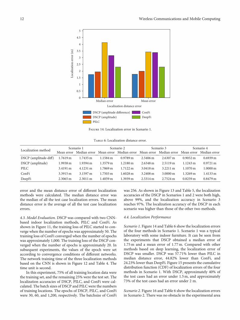
Scenario 1. Figure 14 and Table 6 show the localization errorsof the four methods in Scenario 1. Scenario 1 was a typicallaboratory with some indoor furniture. It can be seen fromthe experiments that DSCP obtained a median error of1.75m and a mean error of 1.77m. Compared with othermethods based on deep learning, the localization error ofDSCP was smaller. DSCP was 57.71% lower than PILC inmedian distance error, 44.82% lower than ConFi, and24.23% lower than DeepFi. Figure 15 presents the cumulativedistribution function (CDF) of localization errors of the fourmethods in Scenario 1. With DSCP, approximately 40% ofthe test cases had an error under 1.5m, and approximately73% of the test cases had an error under 2 m.

Scenario 2. Figure 16 and Table 6 show the localization errorsin Scenario 2. There was no obstacle in the experimental area

Median error Mean errorLocalization distance error

0

0.5

1

1.5

2

2.5

3

3.5

4

4.5

5

Loca

lizat

ion

erro

r (m

)

DSCP (amplitude difference)DSCP (amplitude)PILC

ConFiDeepFi

Figure 14: Localization error in Scenario 1.

Table 6: Localization distance error.

Localization methodScenario 1 Scenario 2 Scenario 3 Scenario 4

Mean error Median error Mean error Median error Mean error Median error Mean error Median error

DSCP (amplitude-diff) 1.7619m 1.7435m 1.1584m 0.9789m 2.5406m 2.6307m 0.9052m 0.6939m

DSCP (amplitude) 1.9938m 1.9394m 1.3579m 1.2180m 2.6348m 2.5119m 1.1243m 0.9721m

PILC 3.4191m 4.1231m 1.7869m 1.7122m 3.0418m 3.2211m 1.1070m 1.0000m

ConFi 3.3915m 3.1597m 1.7503m 1.6028m 3.2408m 3.0000m 1.3269m 1.4133m

DeepFi 2.3065m 2.3011m 1.4059m 1.3939m 2.5314m 2.7524m 0.8259m 0.8479m


of Scenario 2, and there were line of sight (LOS) pathsbetween the transmitter and the receiver. As the experimentsshow in Scenario 2, the DSCP obtained a median error of0.98m and a mean error of 1.16m. DSCP was 42.83% lowerthan PILC in median distance error, 38.93% lower thanConFi, and 29.77% lower than DeepFi. Figure 17 presentsthe CDF of localization errors of the four methods in Sce-nario 2. With DSCP, 55% of the test cases had an error under

1m, and approximately 90% of the test cases have an errorunder 2m.

Scenario 3. Figure 18 and Table 6 show the localization errorsin Scenario 3. Scenario 3 was a typical office with a largenumber of office chairs in the room. The experimental resultsshow that DSCP obtained a median error of 2.63m and amean error of 2.54m. DSCP was 18.33% lower than PILC

Localization error (m)

00 1 2 3 4 5 6

0.1

0.2

0.3

0.4

0.5

0.6

0.7

0.8

0.9

1

CDF

ConFi (epoch=1200)DeepFi

DSCP (amplitude difference)DSCP (amplitude)PILC (epoch=60)

Figure 15: CDF of localization errors in Scenario 1.


0

0.5

1

1.5

2

2.5

Loca

lizat

ion

erro

r (m

)


ConFiDeepFi



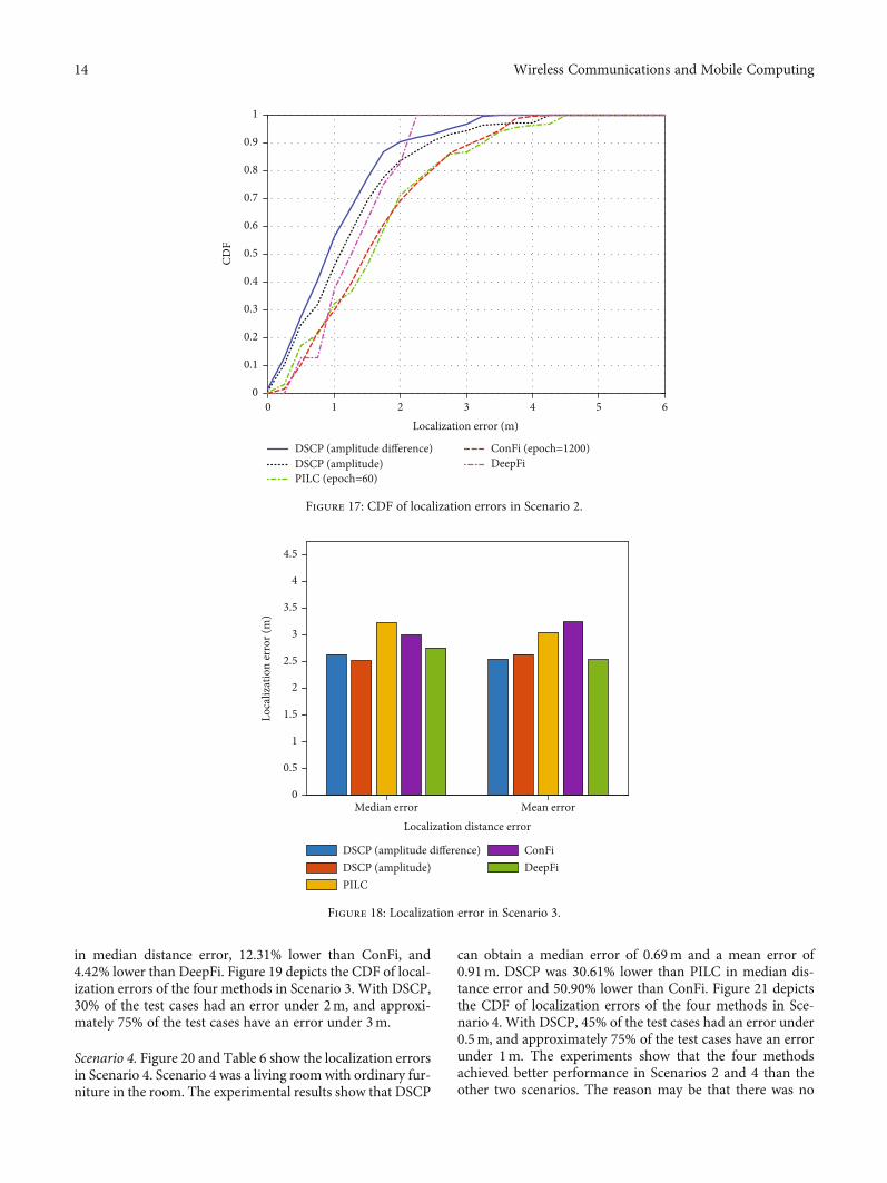
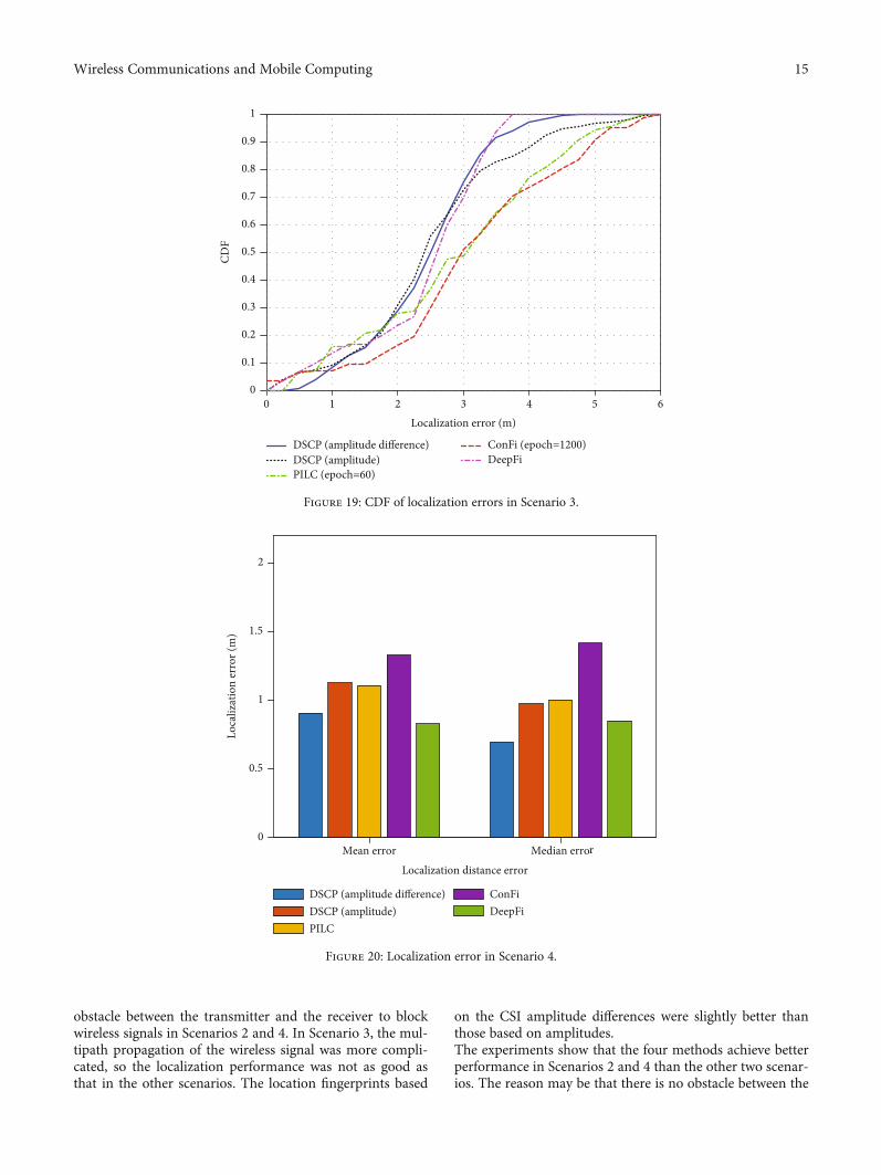
in median distance error, 12.31% lower than ConFi, and4.42% lower than DeepFi. Figure 19 depicts the CDF of local-ization errors of the four methods in Scenario 3. With DSCP,30% of the test cases had an error under 2m, and approxi-mately 75% of the test cases have an error under 3m.

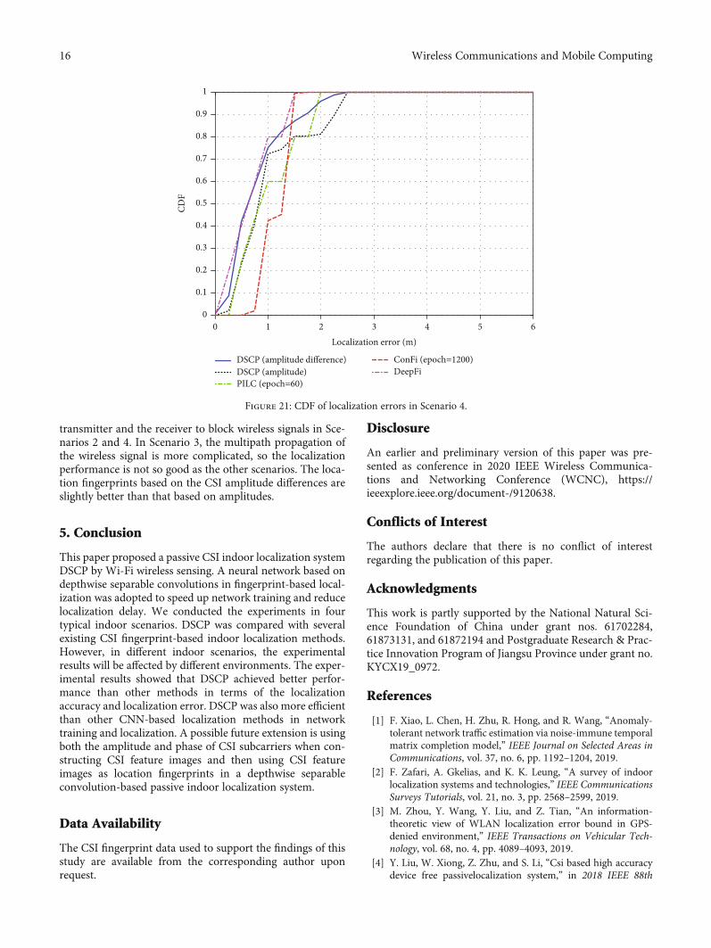
Scenario 4. Figure 20 and Table 6 show the localization errorsin Scenario 4. Scenario 4 was a living room with ordinary fur-niture in the room. The experimental results show that DSCP

can obtain a median error of 0.69m and a mean error of0.91m. DSCP was 30.61% lower than PILC in median dis-tance error and 50.90% lower than ConFi. Figure 21 depictsthe CDF of localization errors of the four methods in Sce-nario 4. With DSCP, 45% of the test cases had an error under0.5m, and approximately 75% of the test cases have an errorunder 1m. The experiments show that the four methodsachieved better performance in Scenarios 2 and 4 than theother two scenarios. The reason may be that there was no


0

0.1

0.2

0.3

0.4

0.5

0.6

0.7

0.8

0.9

1

CDF

0 1 2 3 4 5 6





0

0.5

1

1.5

2

2.5

3

3.5

4

4.5

Loca

lizat

ion

erro

r (m

)


ConFiDeepFi



obstacle between the transmitter and the receiver to blockwireless signals in Scenarios 2 and 4. In Scenario 3, the mul-tipath propagation of the wireless signal was more compli-cated, so the localization performance was not as good asthat in the other scenarios. The location fingerprints based

on the CSI amplitude differences were slightly better thanthose based on amplitudes.The experiments show that the four methods achieve betterperformance in Scenarios 2 and 4 than the other two scenar-ios. The reason may be that there is no obstacle between the


0

0.1

0.2

0.3

0.4

0.5

0.6

0.7

0.8

0.9

1

CDF

0 1 2 3 4 5 6




Mean error Median error

Localization distance error

0

0.5

1

1.5

2

Loca

lizat

ion

erro

r (m

)


ConFiDeepFi



transmitter and the receiver to block wireless signals in Sce-narios 2 and 4. In Scenario 3, the multipath propagation ofthe wireless signal is more complicated, so the localizationperformance is not so good as the other scenarios. The loca-tion fingerprints based on the CSI amplitude differences areslightly better than that based on amplitudes.

5. Conclusion

This paper proposed a passive CSI indoor localization systemDSCP by Wi-Fi wireless sensing. A neural network based ondepthwise separable convolutions in fingerprint-based local-ization was adopted to speed up network training and reducelocalization delay. We conducted the experiments in fourtypical indoor scenarios. DSCP was compared with severalexisting CSI fingerprint-based indoor localization methods.However, in different indoor scenarios, the experimentalresults will be affected by different environments. The exper-imental results showed that DSCP achieved better perfor-mance than other methods in terms of the localizationaccuracy and localization error. DSCP was also more efficientthan other CNN-based localization methods in networktraining and localization. A possible future extension is usingboth the amplitude and phase of CSI subcarriers when con-structing CSI feature images and then using CSI featureimages as location fingerprints in a depthwise separableconvolution-based passive indoor localization system.

Data Availability

The CSI fingerprint data used to support the findings of thisstudy are available from the corresponding author uponrequest.

Disclosure

An earlier and preliminary version of this paper was pre-sented as conference in 2020 IEEE Wireless Communica-tions and Networking Conference (WCNC), https://ieeexplore.ieee.org/document-/9120638.

Conflicts of Interest

The authors declare that there is no conflict of interestregarding the publication of this paper.

Acknowledgments

This work is partly supported by the National Natural Sci-ence Foundation of China under grant nos. 61702284,61873131, and 61872194 and Postgraduate Research & Prac-tice Innovation Program of Jiangsu Province under grant no.KYCX19_0972.

References

[1] F. Xiao, L. Chen, H. Zhu, R. Hong, and R. Wang, “Anomaly-tolerant network traffic estimation via noise-immune temporalmatrix completion model,” IEEE Journal on Selected Areas inCommunications, vol. 37, no. 6, pp. 1192–1204, 2019.

[2] F. Zafari, A. Gkelias, and K. K. Leung, “A survey of indoorlocalization systems and technologies,” IEEE CommunicationsSurveys Tutorials, vol. 21, no. 3, pp. 2568–2599, 2019.

[3] M. Zhou, Y. Wang, Y. Liu, and Z. Tian, “An information-theoretic view of WLAN localization error bound in GPS-denied environment,” IEEE Transactions on Vehicular Tech-nology, vol. 68, no. 4, pp. 4089–4093, 2019.

[4] Y. Liu, W. Xiong, Z. Zhu, and S. Li, “Csi based high accuracydevice free passivelocalization system,” in 2018 IEEE 88th


0

0.1

0.2

0.3

0.4

0.5

0.6

0.7

0.8

0.9

1

CDF

0 1 2 3 4 5 6





https://ieeexplore.ieee.org/document-/9120638

https://ieeexplore.ieee.org/document-/9120638

Vehicular Technology Conference (VTC-Fall), pp. 1–5, Chi-cago, IL, USA, August 2018.

[5] R. Want, A. Hopper, V. Falcão, and J. Gibbons, “The activebadge location system,” ACM Transactions on InformationSystems, vol. 10, no. 1, pp. 91–102, 1992.

[6] F. Xiao, Z. Wang, N. Ye, R. Wang, and X. Li, “One more tagenables fine-grained RFID localization and tracking,”IEEE/ACM Transactions on Networking, vol. 26, no. 1,pp. 161–174, 2018.

[7] P. Dai, Y. Yang, M. Wang, and R. Yan, “Combination of DNNand improved KNN for indoor location fingerprinting,”Wire-less Communications and Mobile Computing, vol. 2019, ArticleID 4283857, 9 pages, 2019.

[8] M. Kotaru, K. Joshi, D. Bharadia, and S. Katti, “Spotfi: decime-ter level localization using wifi,” in Proceedings of the 2015 ACMConference on Special Interest Group on Data Communication,ser. SIGCOMM’15. New York, NY, USA: Association for Com-puting Machinery, pp. 269–282, New York, NY, USA, 2015.

[9] X. Yalong, Z. Shigeng, W. Jianxin, and Z. Chengzhang, “Anovel indoor localization algorithm for efficient mobility man-agement in wireless networks,” Wireless Communications andMobile Computing, vol. 2018, Article ID 9517942, 12 pages,2018.

[10] A. Achroufene, Y. Amirat, and A. Chibani, “RSS-based indoorlocalization using belief function theory,” IEEE Transactionson Automation Science and Engineering, vol. 16, no. 3,pp. 1163–1180, 2019.

[11] P. Bahl and V. N. Padmanabhan, “Radar: an in-building rf-based user location and tracking system,” in Proceedings IEEEINFOCOM 2000. Conference on Computer Communications.Nineteenth Annual Joint Conference of the IEEE Computerand Communications Societies (Cat. No.00CH37064), vol. 2,pp. 775–784, Tel Aviv, Israel, 2000.

[12] Y. Zou,W. Liu, K.Wu, and L. M. Ni, “Wi-Fi radar: recognizinghuman behavior with commodity Wi-Fi,” IEEE Communica-tions Magazine, vol. 55, no. 10, pp. 105–111, 2017.

[13] C. Han, Q. Tan, L. Sun, H. Zhu, and J. Guo, “Csi frequencydomain fingerprint-based passive indoor human detection,”Information, vol. 9, no. 4, p. 95, 2018.

[14] S. Shi, S. Sigg, and Y. Ji, “Probabilistic fingerprinting based pas-sive device-free localization from channel state information,”in 2016 IEEE 83rd Vehicular Technology Conference (VTCSpring), pp. 1–5, Nanjing, China, May 2016.

[15] B. Berruet, O. Baala, A. Caminada, and V. Guillet, “An evalu-ation method of channel state information fingerprinting forsingle gateway indoor localization,” Journal of Network andComputer Applications, vol. 159, p. 102591, 2020.

[16] X. Wang, X. Wang, and S. Mao, “Cifi: deep convolutional neu-ral networks for indoor localization with 5 GHz Wi-Fi,” in2017 IEEE International Conference on Communications(ICC), pp. 1–6, Paris, France, May 2017.

[17] S. Sen, B. Radunovic, R. R. Choudhury, and T.Minka, “You arefacing the Mona Lisa: spot localization using PHY layer infor-mation,” in Proceedings of the 10th International Conferenceon Mobile Systems, Applications, and Services, ser. MobiSys‘12. New York, NY, USA: ACM, pp. 183–196, New York, NY,USA, 2012.

[18] J. Xiao, K. Wu, Y. Yi, and L. M. Ni, “FIFS: fine-grained indoorfingerprinting system,” in 2012 21st International Conferenceon Computer Communications and Networks (ICCCN),pp. 1–7, Munich, Germany, July 2012.

[19] J. Xiao, K. Wu, Y. Yi, L. Wang, and L. M. Ni, “Pilot: passivedevice-free indoor localization using channel state informa-tion,” in 2013 IEEE 33rd International Conference on Distrib-uted Computing Systems (ICDCS), pp. 236–245, Philadelphia,PA, USA, July 2013.

[20] Y. Chapre, A. Ignjatovic, A. Seneviratne, and S. Jha, “CSI-MIMO: an efficient Wi-Fi fingerprinting using Channel StateInformation with MIMO,” Pervasive and Mobile Computing,vol. 23, pp. 89–103, 2015.

[21] H. Abdel-Nasser, R. Samir, I. Sabek, and M. Youssef, “Mono-PHY: mono-stream-based device-free WLAN localization viaphysical layer information,” in 2013 IEEE Wireless Communi-cations and Networking Conference (WCNC), pp. 4546–4551,Shanghai, China, April 2013.

[22] I. Sabek and M. Youssef, “Monostream: A minimal-hardwarehigh accuracy device-free WLAN localization system,” CoRR,p. 11, 2013, https://arxiv.org/abs/1308.0768.

[23] X. Wang, L. Gao, S. Mao, and S. Pandey, “CSI-based finger-printing for indoor localization: a deep learning approach,”IEEE Transactions on Vehicular Technology, vol. 66, no. 1,pp. 763–776, 2017.

[24] X. Wang, L. Gao, and S. Mao, “CSI phase fingerprinting forindoor localization with a deep learning approach,” IEEEInternet of Things Journal, vol. 3, no. 6, pp. 1113–1123, 2016.

[25] H. Chen, Y. Zhang, W. Li, X. Tao, and P. Zhang, “ConFi: con-volutional neural networks based indoor Wi-Fi localizationusing channel state information,” IEEE Access, vol. 5,pp. 18066–18074, 2017.

[26] C. Cai, L. Deng, M. Zheng, and S. Li, “PILC: passive indoorlocalization based on convolutional neural networks,” in2018 Ubiquitous Positioning, Indoor Navigation andLocation-Based Services (UPINLBS), pp. 1–6, Wuhan, China,March 2018.

[27] IEEE, “IEEE Standard for Information technology–Telecom-munications and information exchange between systems Localand metropolitan area networks–Specific requirements Part11: Wireless LAN Medium Access Control (MAC) and Physi-cal Layer (PHY) Specifications,” in IEEE Std 802.11-2012(Revision of IEEE Std 802.11-2007), pp. 1–2793, New York,NY, USA, March 2012.

[28] I. Lu and K. Tsai, “Channel estimation in a proposedIEEE802.11n OFDM MIMO WLAN system,” in 2007 IEEESarnoff Symposium, pp. 1–5, Princeton, NJ, USA, April 2007.

[29] X. Dang, X. Si, Z. Hao, and Y. Huang, “A novel passive indoorlocalization method by fusion CSI amplitude and phase infor-mation,” Sensors, vol. 19, no. 4, 2019.

[30] A. G. Howard, M. Zhu, B. Chen et al., “MobileNets: efficientconvolutional neural networks for mobile vision applications,”CoRR, p. 9, 2017, https://arxiv.org/abs/1704.04861.

[31] J. Wang, H. Jiang, J. Xiong et al., “Lifs: low human467 effort,device-free localization with fine-grained subcarrier informa-tion,” in Proceedings of the 22nd Annual International Confer-ence on Mobile Computing and Networking, ser. MobiCom’16.New York,USA: Association for Computing Machinery,pp. 243–256, New York, NY, USA, 2016.

[32] D. P. Kingma and J. Ba, “Adam: a method for stochastic opti-mization,” 2014, https://arxiv.org/abs/1412.6980.

[33] K. He and J. Sun, “Convolutional neural networks at con-strained time cost,” in 2015 IEEE Conference on ComputerVision and Pattern Recognition (CVPR), pp. 5353–5360, Bos-ton, MA, USA, June 2015.


https://arxiv.org/abs/1308.0768



dscp: depthwise separable convolution-based passive indoor

Documents