dry friction and impact dynamics in railway vehiclesetd.dtu.dk/thesis/58621/imm2501.pdf · dry...
TRANSCRIPT

Dry Friction and Impact Dynamics in Railway Vehicles
Dan Erik Petersen Mark Hoffmannc973539 c973500
M.Sc.Eng. ThesisJune 2003
Supervisor:Hans True
Institute:Informatics and Mathematical ModellingTechnical University of DenmarkRichard Petersens PladsBuilding 321DK-2800 Kongens Lyngby
Denmark

2

Preface
Work on this thesis commenced the 3rd of February and ended the 23rd of June, 2003.The thesis was completed under the supervision of professor Hans True, at the Institutefor Informatics and Mathematical Modelling, Technical University of Denmark. Hisguidance and insight has been both invaluable and inspiring, and we thank him for histime and help, and the opportunity for producing this thesis.
An important portion of work in this project was carried out at Politechnica Warsza-wska, Poland, under the supervision of professor Jerzy Piotrowski and with the help ofArtur Grzelak. Our stay there was rewarding, both culturally and academically, and wewould like to thank them.
Much of the work in this project is based on previous theoretical and numericalwork, and our thanks go out to all those who have contributed to the advancement ofnonlinear dynamics.
Mark Hoffmann Dan Erik Petersenc973500 c973539
23rd June 2003

4 Abstract
Abstract
This thesis develops a methematical model of a Hbbills 311 freight wagon. Central tothis model is the UIC double-link suspension which incorporates a parabolic leaf spring.The lateral and longitudinal dynamical model of the UIC suspension is based on theoryby Jerzy Piotrowski. This model successfully takes into account damping due to dryfriction in the suspension links.
Parameter identification for Piotrowski’s model was performed in Warszaw, Poland,on real UIC double linkages. Two sets of parameters were used, the first emphasizingfrequency-matching characteristics with the experimental setup, and the second match-ing theoretical geometric analysis of the suspension joints. Both were used in simulation.
The vertical dynamical model of the UIC suspension is discussed, and several modelsproposed. Results were generated with the implementation of a piece-wise linear spring-damper system that takes into account the progressive characteristics of the parabolicspring as well as damping due to dry friction.
The wheelsets are constrained by guidance structures of the freight wagon, and theimpacts involving these structures are modelled. Wheel-rail contact forces are calcu-lated using the Shen-Hedrick-Elkins method and a wheel-rail contact geometry table(RSGEO) by Walter Kik.
The wheel profile is the S1002 profile, and the rail profile is the UIC60 profile. Allmodelling and simulation takes place on straight and level track with a fixed gaugeof 1435 mm. Low frequency stability dynamics analysis is carried out. The model isimplemented through C++ programming, accessed through the command line or a JavaGUI, and results analyzed with MatLab .
Keywords: Nonlinear dynamics, railway vehicle dynamics, dry friction, impact dy-namics, differential succession.

Contents
1 Introduction 9
2 Mathematical Model 13
2.1 Wheelset Analysis . . . . . . . . . . . . . . . . . . . . . . . . . . . . . . . 13
2.1.1 Coordinate Systems . . . . . . . . . . . . . . . . . . . . . . . . . . 15
2.1.2 Equations of Motion . . . . . . . . . . . . . . . . . . . . . . . . . 18
2.2 Car Body Analysis . . . . . . . . . . . . . . . . . . . . . . . . . . . . . . 20
2.2.1 Coordinate Systems . . . . . . . . . . . . . . . . . . . . . . . . . . 20
2.2.2 Equations of motion . . . . . . . . . . . . . . . . . . . . . . . . . 22
2.3 Forces . . . . . . . . . . . . . . . . . . . . . . . . . . . . . . . . . . . . . 22
2.4 Complete System . . . . . . . . . . . . . . . . . . . . . . . . . . . . . . . 23
3 Wheel-Rail Contact 25
3.1 RSGEO . . . . . . . . . . . . . . . . . . . . . . . . . . . . . . . . . . . . 25
3.2 Creep Forces . . . . . . . . . . . . . . . . . . . . . . . . . . . . . . . . . . 25
3.3 Normal Forces . . . . . . . . . . . . . . . . . . . . . . . . . . . . . . . . . 27
4 UIC Suspension Links 29
4.1 Model . . . . . . . . . . . . . . . . . . . . . . . . . . . . . . . . . . . . . 29
4.2 Experiment . . . . . . . . . . . . . . . . . . . . . . . . . . . . . . . . . . 31
4.2.1 Measuring Equipment . . . . . . . . . . . . . . . . . . . . . . . . 32
4.2.2 Procedure . . . . . . . . . . . . . . . . . . . . . . . . . . . . . . . 33
4.3 Analysis . . . . . . . . . . . . . . . . . . . . . . . . . . . . . . . . . . . . 34
4.3.1 Problems . . . . . . . . . . . . . . . . . . . . . . . . . . . . . . . 34
4.3.2 Data Fitting Strategy . . . . . . . . . . . . . . . . . . . . . . . . 35
4.3.3 Determining Stiffness . . . . . . . . . . . . . . . . . . . . . . . . . 38
4.3.4 Dry Friction Parameter, T0i . . . . . . . . . . . . . . . . . . . . . 41
4.3.5 Model Parameters . . . . . . . . . . . . . . . . . . . . . . . . . . 41
4.4 Model vs. Measurement . . . . . . . . . . . . . . . . . . . . . . . . . . . 43

6 CONTENTS
5 UIC Vertical Suspension 475.1 Standard Leaf Spring . . . . . . . . . . . . . . . . . . . . . . . . . . . . . 475.2 Parabolic Spring . . . . . . . . . . . . . . . . . . . . . . . . . . . . . . . 525.3 Determining Damping . . . . . . . . . . . . . . . . . . . . . . . . . . . . 54
5.3.1 Standard Leaf Spring . . . . . . . . . . . . . . . . . . . . . . . . . 555.3.2 Parabolic Leaf Spring . . . . . . . . . . . . . . . . . . . . . . . . . 60
6 Impact Model 636.1 Degrees of Freedom . . . . . . . . . . . . . . . . . . . . . . . . . . . . . . 636.2 Mathematical Model . . . . . . . . . . . . . . . . . . . . . . . . . . . . . 64
6.2.1 Impact . . . . . . . . . . . . . . . . . . . . . . . . . . . . . . . . . 646.2.2 Equations . . . . . . . . . . . . . . . . . . . . . . . . . . . . . . . 666.2.3 Forces . . . . . . . . . . . . . . . . . . . . . . . . . . . . . . . . . 66
6.3 Results . . . . . . . . . . . . . . . . . . . . . . . . . . . . . . . . . . . . . 67
7 Freight Wagon Inertia 717.1 Empty Freight Wagon . . . . . . . . . . . . . . . . . . . . . . . . . . . . 717.2 Adding Freight . . . . . . . . . . . . . . . . . . . . . . . . . . . . . . . . 72
8 Dry Friction Dynamics 75
9 Numerical Approach 799.1 Implementation . . . . . . . . . . . . . . . . . . . . . . . . . . . . . . . . 799.2 SDIRK . . . . . . . . . . . . . . . . . . . . . . . . . . . . . . . . . . . . . 809.3 Jacobi Matrix . . . . . . . . . . . . . . . . . . . . . . . . . . . . . . . . . 809.4 Dependencies . . . . . . . . . . . . . . . . . . . . . . . . . . . . . . . . . 83
9.4.1 Front Wheelset . . . . . . . . . . . . . . . . . . . . . . . . . . . . 839.4.2 Rear Wheelset . . . . . . . . . . . . . . . . . . . . . . . . . . . . . 849.4.3 Car Body . . . . . . . . . . . . . . . . . . . . . . . . . . . . . . . 849.4.4 Dry Friction Elements . . . . . . . . . . . . . . . . . . . . . . . . 85
10 Results 8710.1 Method of Attack . . . . . . . . . . . . . . . . . . . . . . . . . . . . . . . 8710.2 Suspension Parameter Set 1 . . . . . . . . . . . . . . . . . . . . . . . . . 88
10.2.1 Critical Velocities . . . . . . . . . . . . . . . . . . . . . . . . . . . 8810.2.2 Guidance Impact Behaviour . . . . . . . . . . . . . . . . . . . . . 94
10.3 Suspension Parameter Set 2 . . . . . . . . . . . . . . . . . . . . . . . . . 11210.3.1 Critical Velocities . . . . . . . . . . . . . . . . . . . . . . . . . . . 11210.3.2 Guidance Impact Behaviour . . . . . . . . . . . . . . . . . . . . . 117
10.4 Frequency Analysis . . . . . . . . . . . . . . . . . . . . . . . . . . . . . . 11910.5 Summary . . . . . . . . . . . . . . . . . . . . . . . . . . . . . . . . . . . 124

CONTENTS 7
11 Future Work 127
12 Conclusion 129
A Symbols 131A.1 Latin Symbols . . . . . . . . . . . . . . . . . . . . . . . . . . . . . . . . . 131
A.1.1 A to B . . . . . . . . . . . . . . . . . . . . . . . . . . . . . . . . . 132A.1.2 C to E . . . . . . . . . . . . . . . . . . . . . . . . . . . . . . . . . 133A.1.3 F to L . . . . . . . . . . . . . . . . . . . . . . . . . . . . . . . . . 134A.1.4 M to Q . . . . . . . . . . . . . . . . . . . . . . . . . . . . . . . . 135A.1.5 R to V . . . . . . . . . . . . . . . . . . . . . . . . . . . . . . . . . 136A.1.6 X to Y . . . . . . . . . . . . . . . . . . . . . . . . . . . . . . . . . 137
A.2 Greek Symbols . . . . . . . . . . . . . . . . . . . . . . . . . . . . . . . . 138
B Parabolic Spring Data 141
C Coordinate Transformations 143
D Creepage 149
E Additional Penetration 153
F Differential Succesion of the Dry Friction Element 157
G Maple Code for the Calculations of the Moment of Inertia 161
H RSGEO table 169
I Java Demonstration 173I.1 Sun Solaris 5.8 . . . . . . . . . . . . . . . . . . . . . . . . . . . . . . . . 173I.2 Apple Mac OS X.2.6 Jaguar . . . . . . . . . . . . . . . . . . . . . . . . . 179

8 CONTENTS

Chapter 1
Introduction
The history of the rail vehicle in Europe is one that stretches back into the 18th century,with the development of first wooden, then steel railed wagonways, on which carts weredrawn with horses. These wagonways evolved into tramways and flanged wheels wereintroduced to rail vehicles in 1789 by William Jessup. In the early 19th century steampower was introduced to these vehicles, and eventually replaced the horse as propulsionpower.
The advent of the modern steam engine by James Watt introduced an instrumentwhich aided rail transportation immensely. With the growth of railways and the trans-portation network they provided, a strong ally in facilitating the industrial revolution,and the spread of industry out in the world had been forged.
Although the long history of rail transportation has seen its ups and downs, thefuture does look promising, with the advent of new technologies such as intermodalfreight trains, and the rise of freight shipments. Shipping rates by rail typically beat thecost of truck shipments, especially over longer distances, and are thus an attractive andimportant instrument of transportation.
Before the strong emergence and interest of nonlinear dynamics, and especially of bi-furcation or catastrophe theory, many decisions involving the design of railway elementsand vehicles resided on sound judgement and engineering skills outside these mathe-matical schools of thought. However, with all man’s pursuits, we push ourselves andour inventions beyond their first conceptions, and into unknown territory. Phenomenaarose which necessitated further study, systematically breaking down the elements of atrain into its constituent parts, modelling these and examining how they behave indi-vidually, collectively, and under different conditions. This mathematical analysis andtesting became possible with the advent of the digital computer, the increasing perfor-mance and availability of computing power and the emergence of numerical algorithms.Phenomena, new and old, which had been observed could now truly be explained or atleast examined mathematically, instead of being rationalized away by sound engineeringexperience.

10 Introduction
The goal of this thesis is to systematically assemble a mathematical model of oneHbbills 311 freight wagon and investigate the behaviour in the low frequency domain.This wagon is illustrated in figure 1.1.
The suspension of the Hbbills 311 is of summary importance in this thesis, since it ischiefly responsible for much of the dynamic behaviour we will investigate. The suspen-sion is dealt with in two chapters, one of which focuses on the longitudinal and lateralcharacteristics, and the other of which focuses on the vertical suspension characteristics.Beyond this, we have also examined a basic dry friction system in order to shed somelight on the behaviour of the UIC suspension.
The important wheel-rail contact interface is modelled through the use of Shen-Hedrick-Elkins theory to determine tangential creep forces, and a tabulated RSGEOdata table in order to determine normal forces and the geometrical parameters aftersuitable dynamic adjustments.
All simulations are performed using S1002 wheel profiles running on UIC60 profilerails canted at 1/40 towards centerline in accordance with what can be found in Europe.The rail gauge is fixed at 1435 mm throughout our experimentation, and we only considerstraight and level track.

11
(a)
(b)
Figure 1.1: (a) The Hbbills 311 freight wagon. The internal partition walls are clearly visible. (b)Schematic of the Hbills 311 freight wagon.

12 Introduction

Chapter 2
Mathematical Model
In this chapter we derive our mathematical model of the Hbbills 311 freight wagon. Wemodel the freight wagon as a multi body system consisting of two wheelsets and a carbody. Through an analysis of each element we set up a nonlinear system of ordinarydifferential equations that determines the motion of the vehicle.
The interacting forces such as contact forces between wheel and rail, suspension forcesand impact forces play a central role in the dynamics of the freight wagon, however, inorder to present the mathematical model of the freight wagon as simple as possible theinteracting forces are referred to through mathematical symbols, whereas the modellingof these forces are omitted this chapter. The modelling of the interacting forces is thetopic of chapters to come.
In figure 2.1 we have shown model pictures of the freight wagon emphasizing themain elements that are important in the mathematical modelling. We refer to appendixA for detailed information of all defined quantities. A few constants we use are givenvalues in table 2.1. We have used the symbol shown in figure 2.2 as a suspensionelement. The purpose of this is to have an abstract suspension element allowing multiplesuspension implementations exhibiting elements such as linear springs/dampers, UIClinks, leaf springs and parabolic springs without changing the overall structure of themathematical model and, ultimately, the construction of the computer program used tosolve the mathematical model.
2.1 Wheelset Analysis
In general, a rigid body has six degrees of freedom. Three coordinates to specify theposition of the center of mass and three coordinates to specify the rotation of the bodyaround its principal axes. However, the configuration space for a real wheelset is notsix dimensional, because the wheelset is constrained (if derailment is neglected) to bein contact with the rails. This constraint connects the lateral and yaw motion with the

14 Mathematical Model
������������������������
������������������������
��������������
��������������
��������������
��������������
��������
��������
��������
��������
��������
��������
��������
��������
���������
���������
���������
���������
��������������
��������������
��������������
��������������
��������
��������
��������
��������
��������
��������
��������
��������
Guidance
Center of Mass
x
y zCenter of Mass
Center of Mass
l
b
(a) Top view.
������������
������������
����������������
����������������
����������������
����������������
z
yx
Center of Mass
��������������������
��������������������
��������������������
��������������������
Center of Mass
Guidance
h
b
(b) Front view.
Figure 2.1: Model pictures of the Hbbills 311.
���������������
���������������
Figure 2.2: General suspension element.

2.1 Wheelset Analysis 15
Parameter Value Unit
b 1.074 [m]h 0.802∗ [m]l 5.00 [m]mw 1022 [kg]mc 13563∗ [kg]Iwx 678 [kg m2]Iwy 80 [kg m2]Iwz 678 [kg m2]Icx 32675∗ [kg m2]Icz 413097∗ [kg m2]g 9.82 [m/s2]
Table 2.1: Some central constants used in the report. Values marked with ∗ are for an empty wagon.
vertical and roll motion of the wheelset.Instead, in modelling wheelsets one can choose to proceed in another fashion. We
have followed the strategy from [9]. This model allows the wheelset to have six degreesof freedom leaving out the kinematic wheel-rail constraint discussed above and we thusavoid having a differential algebraic system to solve. Instead of the constraint, thewheelet penetrates into the rail making the contact forces between the wheel and rail afunction of the penetration. Thus, the wheelset has the following degrees of freedom
x : Wheelset longitudinal
y : Wheelset lateral
z : Wheelset vertical
φ : Wheelset roll
χ : Wheelset pitch
ψ : Wheelset yaw
2.1.1 Coordinate Systems
We have found it necessary to define three different coordinate systems regarding themotion of the wheelset. Following the usual conventions in railway dynamics we define arotation around a longitudinal axis as roll (φ), lateral axis as pitch (χ) and vertical axisas yaw (ψ) (see figure 2.4). Furthermore, transformation matrices between all definedcoordinate systems are derived and listed in appendix C.

16 Mathematical Model
• (Xr, Yr, Zr)A reference frame moving along with the velocity of the vehicle. The subscript isfor rail. Each wheelset has its own rail coordinate system and the origin is placedin the center of mass of the wheelset when it is in centered position. This frameis an inertial frame of reference. Positive directions are defined in figure 2.3(a).
• (Xw, Yw, Zw)A coordinate system that follows the wheelsets. The subscript is for wheelset. Thecoordinate axes are parallel to the principal axes of the wheelset. Each wheelsethas its own wheelset coordinate system and the origin is placed in the center ofmass. This frame is not an inertial frame of reference. Positive directions aredefined in figure 2.3(b).
• (Xc, Yc, Zc)A coordinate system that follows the contact plane between the wheel and rail. Thesubscript is for contact. The origin is placed in the contact point, see figure 2.3(c).The contact coordinate system is defined because it is a natural reference whenthe contact forces are going to be described.

2.1 Wheelset Analysis 17
Vzr
yrxr
φ
Center of track
right left
(a) Rail coordinate system.
zw
ywxw
right left
Center of mass
(b) Wheelset coordinate system.
δrδ l
ycxc
zcyc
xc
zc
right left
(c) Contact coordinate system for the leftand right wheel.
Figure 2.3: Wheelset coordinate systems.
z
x
yφ
ψ
χ
Figure 2.4: Positive directions for the angles (right hand rule).

18 Mathematical Model
2.1.2 Equations of Motion
We determine the position of the center of mass of the wheelset by using Newton’ssecond law, whereas the rotation of the wheelset is found through Euler’s equations ofmotion. The application of Newton’s second law is straight forward, because we canset up the equations of motion in the rail reference frame, which is an inertial frame ofreference. The results of this is
mwx =∑
F rx,ext
mwy =∑
F ry,ext
mwz =∑
F rz,ext
However, to determine the rotation of a rigid body in a three dimensional space we haveto be more careful. It is seen that the wheelset coordinate system is not an inertial frameof reference, and the consequence of this is that gyroscopic forces has to be taken intoconsideration. The result of this is formulated in Euler’s equations of motion. Theseequations are derived as follows.
The angular momentum around the center of mass and according to the principalaxes of the wheelset is given by
LC = Iwxφ · ewx + Iwyχ · ewy + Iwzψ · ewzThe theorem of angular momentum says that
dLC
dt= τC,ext
and since the wheelset coordinate system is rotating we find that
dLC
dt= Iwxφ · ewx + Iwyχ · ewy + Iwzψ · ewz
+Iwxφ · dewxdt
+ Iwyχ · dewydt
+ Iwzψ · dewzdt
Keeping in mind that the angular velocity of the wheelset coordinate system is ω =[φ, 0, ψ]T we find that
dewxdt
= ω × ewx
dewydt
= ω × ewy
dewzdt
= ω × ewz

2.1 Wheelset Analysis 19
thus
dLC
dt= Iwxφ · ewx + Iwyχ · ewy + Iwzψ · ewz + ω × LC
=
Iwxφ− Iwyχψ
Iwyχ + (Iwx − Iwz)φψ
Iwzψ + Iwyφχ
· ewx
ewyewz
From this we find that Euler’s equations takes the form
Iwxφ = Iwyχψ +∑
τwx,ext
Iwyχ = (Iwz − Iwx)φψ +∑
τwy,ext
Iwzψ = −Iwyφχ+∑
τwz,ext
The order of φ and ψ is about 10−2 or less, and χ ≈ V/r0, where V is the velocity ofthe vehicle and r0 is the known as the basic rolling radius of the wheels. We immedi-ately neglect the (Iwz − Iwx)φψ term due to the multiplication of two low order terms.Furthermore, if we consider a simulation at V = 30 m s−1 (r0 = 0.425 m) we find that
|Iwyχψ| < 80 · 71 · 10−2 = 56.8
| − Iwyφχ| < 80 · 10−2 · 71 = 56.8
which is much less than the magnitude of the moments due to the contact, suspensionand impact forces, and thus we neglect these terms as well. Leaving out the gyroscopicforces we determine the motion of the wheelset through the following nonlinear systemof equations.
mwx = Crlx + Cr
rx + Srlx + Sr
rx + δrlx + δr
rx (2.1)mwy = Cr
ly + Crry + Sr
ly + Srry + δr
ly + δrry (2.2)
mwz = Crlz + Cr
rz + Srlz + Sr
rz −mwg (2.3)Iwxφ = alC
wlz − arC
wrz + b(Sw
lz + δwlz) − b(Sw
rz + δwrz) (2.4)
Iwyχ = −rlCwlx − rrC
wrx (2.5)
Iwzψ = −alCwlx + arC
wrx − b(Sw
lx + δwlx) + b(Sw
rx + δwrx) (2.6)
where C, S and δ are short for contact, suspension and impact forces, respectively. Theimpact forces are assumed to act in a plane parallel to flat earth.
Equation (2.1) to (2.6) completely defines the position of the wheelset. We cansimplify the system slightly, because we are not interested in distinguishing a situationwith χ1 wheelset revolutions from another situation with χ2 wheelset revolutions. Thusχ in itself is uninteresting, yet χ is very important since the contact forces depend on

20 Mathematical Model
the relative velocity between the wheel and rail. Since χ ∼ Vr0
we can simplify this aswell. We define a pitch angular velocity perturbation, β, as the deviation from the idealrolling velocity ( V
r0):
χ =V
r0+ β
thus equation (2.5) is reduced to
Iwyβ = −rlCwlx − rrC
wrx
2.2 Car Body Analysis
The motion car body is affected by wheelset through suspension forces and impactforces. However, since the inertia of the car body is very big compared to the wheelsetswe neglect the longitudinal and pitch motion of the car body. With this simplificationwe are left with the following four degrees of freedom
y : Car body lateral
z : Car body vertical
φ : Car body roll
ψ : Car body yaw
2.2.1 Coordinate Systems
To be able to set up the equations of motion for the car body we now define two referenceframes.
• (Xr, Yr, Zr)A reference frame moving along with the velocity of the vehicle. The subscript isfor rail. The car body has its own rail coordinate system and the origin is placedin the center of mass of the car body whent it is in centered position. This frameis an inertial frame of reference. Positive directions are shown in figure 2.5(a).
• (Xb, Yb, Zb)A coordinate system that follows the car body. The subscript is for car body. Thecoordinate axes are parallel to the principal axes of the car body. The origin isplaced in the center of mass of the car body. Positive directions are shown in figure2.5(b).
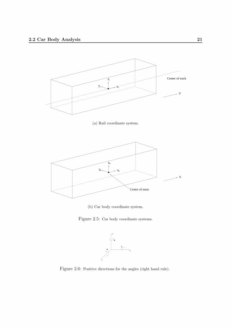
2.2 Car Body Analysis 21
yr
zr
xr
V
Center of track
(a) Rail coordinate system.
yb
zb
xb
V
Center of mass
(b) Car body coordinate system.
Figure 2.5: Car body coordinate systems.
z
x
yφ
ψ
χ
Figure 2.6: Positive directions for the angles (right hand rule).

22 Mathematical Model
2.2.2 Equations of motion
We follow the same strategy as before, however, since the order of φ, χ and ψ are allvery small we can neglect gyroscopic effects immediately. Thus, the motion of the carbody is determined from
mcy =∑
F ry,ext
mcz =∑
F rz,ext
Icxφ =∑
τ bx,ext
Iczψ =∑
τ bz,ext
leading to
mcy = Srfly + Sr
fry + Srrly + Sr
rry + δrfly + δr
fry + δrrly + δr
rry (2.7)mcz = Sr
flz + Srfrz + Sr
rlz + Srrrz −mcg (2.8)
Icxφ = h(Sbfly + Sb
fry + Sbrly + Sb
rry + δbfly + δb
fry + δbrly + δb
rry) (2.9)
+b(Sbflz − Sb
frz + Sbrlz − Sb
rrz + δbflz − δb
frz + δbrlz − δb
rrz) (2.10)
Iczψ = b(−Sbflx + Sb
frx − Sbrlx + Sb
rrx − δbflx + δb
frx − δbrlx + δb
rrx) (2.11)
+l(Sbfly + Sb
fry − Sbrly − Sb
rry + δbfly + δb
fry − δbrly − δb
rry) (2.12)
2.3 Forces
The forces involved in the system arise from 3 different characteristic locations : wheel-rail contact, suspension forces and impact forces between the wheelset and car bodyguidance structures. In our equations, we have labelled wheel-rail contact forces as C,the suspension forces as S and the impact forces as δ.
The superscripts prevalent among these force symbols indicate what coordinate sys-tem the value represented by the symbol is measured in. Here we have that w indicatesthe wheelset coordinate system, b the car body coordinate system and r indicates therail coordinate system.
Subscripts first indicate if the force is generated on the right, r, or left, l, side ofthe freight wagon, i.e. the right and left wheel or suspension element. They secondlyindicate with what direction they are measured in, with x, y and z being the directionsin the corresponding coordinate system.
Furthermore, the car body forces subscripts are prefixed by either f or r, in order toindicate if forces originate from the front or rear wheelset. The mathematical modelsthat reside behind all these forces are described in the chapters to come.

2.4 Complete System 23
2.4 Complete System
y1 Front wheelset longitudinal y31 T1 UIC, front left longitudinaly2 Front wheelset longitudinal velocity y32 T2 UIC, front left longitudinaly3 Front wheelset lateral y33 T3 UIC, front left longitudinaly4 Front wheelset lateral velocity y34 T4 UIC, front left longitudinaly5 Front wheelset vertical y35 T1 UIC, front right longitudinaly6 Front wheelset vertical velocity y36 T2 UIC, front right longitudinaly7 Front wheelset roll y37 T3 UIC, front right longitudinaly8 Front wheelset roll angular velocity y38 T4 UIC, front right longitudinaly9 Front wheelset pitch ang. vel. pert. y39 T1 UIC, rear left longitudinaly10 Front wheelset yaw y40 T2 UIC, rear left longitudinaly11 Front wheelset yaw angular velocity y41 T3 UIC, rear left longitudinaly12 Rear wheelset longitudinal y42 T4 UIC, rear left longitudinaly13 Rear wheelset longitudinal velocity y43 T1 UIC, rear right longitudinaly14 Rear wheelset lateral y44 T2 UIC, rear right longitudinaly15 Rear wheelset lateral velocity y45 T3 UIC, rear right longitudinaly16 Rear wheelset vertical y46 T4 UIC, rear right longitudinaly17 Rear wheelset vertical velocity y47 T UIC, front left lateraly18 Rear wheelset roll y48 T UIC, front right lateraly19 Rear wheelset roll angular velocity y49 T UIC, rear left lateraly20 Rear wheelset pitch ang. vel. pert. y50 T UIC, rear right lateraly21 Rear wheelset yaw y51 Leaf spring, front left verticaly22 Rear wheelset yaw angular velocity y52 Leaf spring, front right verticaly23 Car body lateral y53 Leaf spring, rear left verticaly24 Car body lateral velocity y54 Leaf spring, rear right verticaly25 Car body verticaly26 Car body vertical velocityy27 Car body rolly28 Car body roll angular velocityy29 Car body yawy30 Car body yaw angular velocity
Table 2.2: Table detailing the independent variables in the system.
We define our complete system as the following system of nonlinear first order ODE ’s.
y = f(y) y = [y1, y2, . . . , y30]T Suspension type 1
y = f(y) y = [y1, y2, . . . , y50]T Suspension type 2
y = f(y) y = [y1, y2, . . . , y54]T Suspention type 3
(2.13)

24 Mathematical Model
The right hand side f is a vector function defined by the previous analysis of the elementsin freight wagon. In table 2.2 it is possible to see a describtion of yi. Furthermore, anexplanation of the different suspension types is listed below
• Suspension type 1: Linear model. All suspension elements are linear spring-dampers.
• Suspension type 2 : UIC links are present in the lateral and longitudinal dynam-ics. A stepwise linear spring-damper represents a parabolic spring in the verticaldynamics.
• Suspension type 3 : Standard leaf spring model. UIC links are present in thelateral and longitudinal dynamics. A standard leaf spring represents the verticaldynamics.

Chapter 3
Wheel-Rail Contact
3.1 RSGEO
The contact forces between the wheels and rails play a crucial role when analysing thedynamics of railway vehicles. In order to get a realistic model of the contact forces,[4] has tabulated the geometrical parameters1 between the UIC60 rail profile and theS1002 wheel profile through the use of RSGEO, developed by W. Kik. In general, thesegeometrical parameters depend on the lateral displacement of the wheelset as well as theyaw motion of the wheelset. The effect of the yaw motion of the wheelset is an additionallongitudinal displacement of the contact point, but in simulations with curve radii largerthan 200 m this effect is negligible (see [7]). In this project we only consider simulationson a straight and level track, and therefore our geometrical parameters depend only onthe lateral displacement of the wheelset.
The strength of the RSGEO table is that we do not have to compute the geometricalparameters during the simulation, because it is tabulated beforehand. However, thetable has a certain resolution, which means that we have to do something when we havea lateral displacement of the wheelset in between the table values. We have chosen asimple linear interpolation strategy to get around this problem, and we find it reasonablesince the resolution of the table is quite dense2. In appendix H we have illustrated thegeometrical parameters in order to get a feeling of the data stored in the RSGEO table.
3.2 Creep Forces
In this section we will find expressions for the tangential wheel-rail forces, called creepforces, that arise in the wheel-rail contact patch. Since the wheel-rail interaction is very
1i.e. rolling radius, position of contact point, size of contact patch, etc.2table entry every 10−5 m of lateral displacement.

26 Wheel-Rail Contact
important when analysing the behaviour of the vehicle, we have to take into accountsome of the nonlinearities that exist in this contact.
Several theories have been developed to approximate the creep forces, and the onewe use is due to Shen, Hedrick and Elkins (SHE). The method combines Kalker’s lineartheory with the theory presented by Johnson and Vermuelen, and the result is a nonlinearrelationship between the creep forces and the normal forces.
To be able to use SHE we have to find the relative motion between the wheel andrail. This relative motion is called the creepage. This requires some mathematical ma-nipulation which can be found in appendix D. We use SHE because the approximationof the creep forces is good compared to real measurements and it is well suited for dy-namic simulations. This well suitedness is due to the fact that SHE consists of explicitformulas. This results in creep force calculations that are very fast compared to iterativemethods. We have found the following creep terms.
ξlx = 1 − rlχ
V+x− alψ
V
ξrx = 1 − rrχ
V+x+ arψ
V
ξly =
(−ψ +
y + rlφ
V
)cos δl +
z + alφ
Vsin δl
ξry =
(−ψ +
y + rrφ
V
)cos δr − z − arφ
Vsin δr
ξls =−χ sin δl + ψ cos δl
V
ξrs =χ sin δr + ψ cos δr
V
Kalker’s linear theory gives the following creep force components with respect to thecontact coordinate system
Fx = −aebeGC11ξx
Fy = −aebeG(C22ξy +
√aebeC23ξs
)and the resulting creep force is then
Fτ = Fxex + Fyey
where G is the shear modulus3 and C11, C22 and C23 are Kalker’s creepage coefficients.These coefficients are also provided by the RSGEO table. We adjust the creep forcefrom Kalker’s linear theory and the result are the creep forces Fx and Fy, given by
3G = 21·1010
2·(1+0.27)Nm2 ≈ 8.27 · 1010 N
m2

3.3 Normal Forces 27
|Fτ | =
µN
([|Fτ |µN
]− 1
3
[|Fτ |µN
]2+ 1
27
[|Fτ |µN
]3) |Fτ |µN
< 3
µN |Fτ |µN
≥ 3
(3.1)
ε =|Fτ ||Fτ |
Fx = εFx Fy = εFy
The friction coefficient µ described here is chosen to be 0.15 throughout our simulations.The creep versus creep force relationship given in equation (3.1) is in general not realisticsince the creep force will decay when the wheels are spinning, but since we do not haveany torque on the wheel axles we can accept the above relationship.
3.3 Normal Forces
The normal forces generated at the contact points arise directly from Newton’s thirdlaw: every action force has an equal and opposite reaction force. We also consider thewheel and rail to be two elastic bodies, and are thus subject to deformation. In order tomodel the actual deformation, we consider the two bodies to penetrate into one anotherwithout deforming, and use the fact that the normal force depends on this fictitiouspenetration.
In our effort to determine the normal forces, we are then required to somehow de-termine characteristics of the contact patch, most especially penetration. Ultimately,to determine the normal force, we take advantage of a relationship between wheel-railpenetration and the normal forces generated.
Our first step is the use of theory presented by Henrich Hertz in the late 19th century(1882) in order to determine contact patch characteristics. This enables us to begin todetermine the forces by letting us know the dimensions of the elliptic contact patchbetween the wheel and rail. This, however, comes under the price of the following fourconditions:
• The two bodies in contact must be described by a bilinear polynomial in the pointof contact.
• The two bodies are made from completely elastic, homogeneous and isotropicmaterials.
• The displacement in the point of contact can be neglected.
• The diameter of the contact patch is small compared to the characteristic diametersof the two bodies.

28 Wheel-Rail Contact
By [4], the relationship between contact patch ellipse semi-axes and penetration withrespect to the normal force generated is given by:
ae ∝ N13 be ∝ N
13 N ∝ q
32
RSGEO yields the static4 normal force as a function of the lateral displacement ofthe wheelsets. We then adjust the normal force and the contact ellipse geometriesdynamically, because the rolling motion and the vertical displacements of the wheelsetswill affect the normal force. We do this by using that the above proportionalities yieldthe following formula for updating the normal force:
N0 = kq320
Ndyn = kq32dyn
qdyn = q0 + ∆q
ThusNdyn
N0=
[qdyn
q0
] 32
=
[q0 + ∆q
q0
] 32
Ndyn = N0
[1 +
∆q
q0
] 32
where ∆q is the additional penetration given by (see appendix E):
∆ql = −(aRl − y − al − φrl) sin(δl + φ) + (−z − φal) cos(δl + φ)∆qr = (−aRr − y + ar − φrr) sin(δr − φ) + (−z + φar) cos(δr − φ)
Similary, we update the contact ellipse by
ae,dyn = ae,0
[Ndyn
N0
] 13
be,dyn = be,0
[Ndyn
N0
] 13
4The normal force when the wheelset is not influenced by external forces except the contact forcesand gravity.

Chapter 4
UIC Suspension Links
The UIC link suspension comes in a variety of configurations, but the type that weare interested in here is known as the double-link kind, and is used by many freightwagons in Europe. Figure 4.1 illustrates the entire suspension set up for one side of awheelset. Figure 4.2 illustrates the double links that characterize this suspension, andwhich governs the lateral and longitudinal dynamics of the suspension. The verticalspring in these images is a standard leaf spring, and it should be noted again that thevertical spring on the Hbbills 311 is a parabolic spring.
The good properties of the link suspension is that it delivers stiffness as well asdamping in an very economic fashion. The stiffness comes into play due to the rise inpotential energy for any displacement from equilibrium much like the stiffness presentin an ordinary pendulum. The damping in the link suspension is a consequence of thedry friction that occurs in the joints. However, this dissipation of energy is only presentwhen the amplitude of the excitations exceeds a certain limit. This means that for smallexcitations the joints experience pure rolling (at least in theory) for which there is noloss in energy. This critical value differentiating the rolling motion and sliding motion ofthe joints depends on many factors such as the dimensions of the joints, weather, stateof wear, on so on.
The UIC link suspension exhibits also some undesirable properties. Firstly, thelateral dynamics of the suspension is not satisfactory even though the speed of thevehicle is moderate. Secondly, the dynamics of the vehicle depends highly on the stateof the suspension. This state changes significantly with wear, weather conditions anddirt and grime, for example.
4.1 Model
We have used the mathematical model presented by Jerzy Piotrowski (see [8]) to modelthe lateral and longitudinal dynamics of the UIC suspension. The model is composed

30 UIC Suspension Links
Figure 4.1: Model picture of the UIC double link suspension with the standard leaf spring.
Figure 4.2: UIC double links.
k1 T01
k
m
Figure 4.3: Lateral model of the UIC suspension.
k1 T01
k2 T02
k3 T03
k4 T04
k
m
Figure 4.4: Longitudinal model of the UIC suspension.

4.2 Experiment 31
of linear springs and dry friction sliders (see figure 4.3 and 4.4).A significant property of this model by Piotrowski is that the stiffnesses of the pa-
rameters in the model are assumed to vary linearly with respect to the load that thesuspension supports. Thus in this chapter we ultimately determine a set of normalizedparameters, which can be scaled to correct values depending on how much load thesuspension supports.
Another consequence of the model that we adopt is that we assume Coulomb’s law offriction holds for sliding in the joints. This has been argued for in [8], and a comparisonof measurement with the theoretical curve for Coulomb’s friction law can be see infigure F.2 in the appendix. As can be seen, there seems to be an acceptable degree ofsimilarity. Ultimately, this entails that we do not differentiate between static and kineticcoefficients of friction when it comes to sliding in the suspension joints.
The mathematical model is derived through a differential succesion of the dry frictionelement. A derivation1 of this is found in appendix F and the result is summarized below.
F = −ky + T1 Lateral
F = −ky +4∑i=1
Ti Longitudinal
where Ti are defined by
Ti =
−kiy if |Ti| < T0i
− [kiy]+ if Ti = T0i
[−kiy]+ if Ti = −T0i
The parameters k, ki and T0 are determined through real experiments on the UICsuspension. The experiments and identification of the parameters is the topic of thefollowing sections.
4.2 Experiment
The aim of this section is to produce a set of parameters for the lateral and longitudinaldynamics of the UIC suspension model. Actual experimental measurements were carriedout at the Institute of Vehicles, Warsaw University of Technology, in the month of March,2003, in cooperation with Artur Grzelak and under the guidance of Jerzy Piotrowski.
As inspired by [8], we focus mainly on the longitudinal and lateral dynamics ofthe UIC suspension here, and thus it is sufficient for us to create a setup involvingonly the actual linkages present in the UIC suspension, omitting the leaf spring. Thelinkages were delivered in a worn state as desired, but in that they were disassembled,
1This technique is known in non-smooth mechanics but this derivation is not shown in [8].

32 UIC Suspension Links
it was impossible to determine the exact original configuration of the linkages. Unableto assemble the linkages as they originally fit together, we had no other option but tosandblast and reprofile the linkages in an attempt to yield them as new in order toattempt meaningful experimentation with them.
Furthermore, in that the leaf spring is of no interest in our measurements, it is re-placed by a stiff beam upon which mass is placed in order to load the linkages. Theactual construction of the suspension setup is peformed in an upside down fashion, in-spired by [8]. This setup is illustrated in figure 4.5. The mass of the beam and addedmasses total 378.2 kg. This value has remained constant throughout experimentation.The length of the beam replacing the leaf spring is 1.22 m. The angle α = 25.9◦ repre-sents the angle the linkages form with respect to vertical. The UIC linkage dimensionscorrespond to those where the longitudinal pivot element has a diameter of 35 mm.
Figure 4.5: The suspension setup.
4.2.1 Measuring Equipment
The suspension setup was instrumented with linear displacement sensors in the longi-tudinal and lateral directions. They operate on the basis of translating physical dis-placement into a voltage value that is subsequently transmitted to an amplifier. Theamplifier then feeds the analog signal to an analog to digital converter that interfaceswith the computer through a PCI card device, and the digital signal is subsequentlyrecorded by software. The displacement sensors can be seen in figure 4.5.
A brief overview of the measurement equipment:

4.2 Experiment 33
• 2 linear displacement sensors.
• Amplifier.
• Analog to digital converter.
• Computer with available PCI slot.
• Oscilloscope software for sampling data.
4.2.2 Procedure
We here outline the procedures taken to setup the oscilloscope software correctly formeasurement. This must be done for both sensors.
1. Ensure that the suspension is at rest.
2. Select the channel for the sensor of interest.
3. Shift the sensor physically such that it registers a voltage corresponding to themiddle of the range of voltage it is capable of generating (its own zero-point).
4. Set the oscilloscope software’s zero-point for the voltage given by the sensor ofinterest.
5. Utilizing a standardized block of metal with a known dimension, insert this be-tween the sensor and suspension, taking care not to displace the suspension.
6. Set the oscilloscope software to register the voltage now measured.
7. The oscilloscope software is calibrated by entering the displacement in mm corre-sponding to the standardized block of metal.
8. Repeat for the other sensor.
Once this is done, we can proceed to limit ourselves to measure only two channelsof the sixteen that the digital to analog converter delivers. We also choose the totalmeasurement time to record. In recording, the sampling was done at a rate of 1000samples per second.
Recordings were performed in one direction at a time, since the mathematical modelwe strive to implement explicitly separates longitudinal and lateral mathematical ele-ments. Theoretically, they should be kinematically independent. However, in measure-ment, we are interested in preventing as much dissipation as possible other than thatdissipation that will yield parameters for the mathematical model. This is because thatlow amplitude oscillations do not seem to be nearly as kinematically independent as

34 UIC Suspension Links
the larger amplitude oscillations. This leads to the low amplitude pure rolling oscilla-tions to die off too quickly for proper measurement if oscillation goes on laterally andlongitudinally simultaneously.
When recording starts, the suspension is excited in the lateral direction, carefullypreventing too much excitation in the longitudinal direction. This is done to an ampli-tude that takes advantage of the entire range of motion the corresponding sensor canregister. Furthermore, excitation of the suspension ceases prior to the suspension reach-ing an extremum in motion. This is of importance when we later need to determineparameters from measurements. An analogous procedure was used for measurement inthe longtitudinal direction.
Several measurements were recorded for excitations in both longtitudinal and lateraldirections in order to limit the data from a poor measurement run polluting calculatedparameters.
Once a recording is done, it can be saved in its raw format to disk, but in order toanalyse results, the data is converted to ASCII format, and only every 5th data point issampled. This reduces both the file sizes as well some high frequency noise in the data.
4.3 Analysis
In order to analyse results, we export measurements into ASCII files which are easierto manipulate and extract data from. Also, when the oscilloscope software convertsmeasurements to ASCII files, the original voltage data from the sensors are automaticallytransformed into displacements according to the calibration done earlier.
The result of a typical experiment is shown in figure 4.6. The time histories shownconsists of three different stages. The first stage shows how we have excited the sus-pension at resonance frequency in order to displace the suspension from equilibrium.We then stop pushing it (at about t = 3 s in the longitudinal experiment and t = 2.5s in the lateral experiment) and record approximately 15 seconds of motion all in all.The second stage is the damping transient which is eventually quickly taken over by the“pure” rolling motion in the joints (we see a little dissipation in this motion as well).
In the following sections we are going to describe how we extract the model param-eters from the time histories measured.
4.3.1 Problems
It becomes evident, that although the mathematical model of the UIC suspension hasfour dry friction sliders in order to account for longitudinal behaviour, the stiffnesses ofthe springs for the individual sliders can not be determined at first glance. Dissipationis so strong in the suspension that it resides most of the time in either all joints rolling,or all joints sliding. Determining the exact moments in which certain joints transition

4.3 Analysis 35
0 5 10 15−0.015
−0.01
−0.005
0
0.005
0.01
0.015
0.02
Time [s]
Dis
plac
emen
t [m
]
Longitudinal Experiment
(a) Longitudinal.
in0 5 10 15
−0.04
−0.03
−0.02
−0.01
0
0.01
0.02
0.03
0.04
0.05
Time [s]
Dis
plac
emen
t [m
]
Lateral Experiment
(b) Lateral.
Figure 4.6: Measured results for one of the experiments.
from rolling to sliding is practically impossible. Therefore in the longitudinal case wewill only be able to determine the stiffness k exhibited when all joints are sliding, as wellas the total stiffness of the system when all joints are rolling. This will let us determine∑ki, the sum of the stiffnesses of the springs connected with dry friction sliders. In the
lateral case, we only have one slider/spring element and∑ki = k1.
4.3.2 Data Fitting Strategy
In observing the time series, we see that there are two characteristic frequencies which wewish to extract. This holds for both longitudinal and lateral excitation measurements.These frequencies characterise the suspension when all joints are sliding, and when alljoints are rolling. The condition in which all joints are rolling is visible towards thelater stages in the time series, when the amplitude of excitation is only being weaklydissipated. However, the condition in which all joints are sliding is more difficult toextract. These frequencies will be used to establish the stiffnesses of the springs in themathematical model of the UIC suspension.
Sliding
This condition of all joints sliding occurs during the time when maximum dissipation ofthe amplitude is taking place. If we observe a single extremum of the motion prior topure rolling, we can be sure that all joints will stick as soon as the velocities of movementin the joints become zero just when the motion reaches the extremum. After this, thesuspension joints will progressively cascade into pure sliding as the motion transitions toan opposite extreme. However, prior to the extremum, pure sliding occurs in all joints.

36 UIC Suspension Links
Therefore our strategy becomes one in isolating a section of the time series wherepure sliding occurs in all joints. This will be from the point of an extrema, and movingback in time a certain amount. This amount is arbitrary, however we limit it to movingback so far as we don’t return to a displacement in which pure rolling will take overlater in the time series. Thus we define a cutoff amplitude to prevent us from takingtoo great a section of the time series for analysis. This will avoid us having a section foranalysis in which one or more joints may be rolling.
Once we have agreed on a section of the time series where all joints are sliding, wefit this curve with a sine function of the following form:
f(t) = a sin(ωslidingt+ φ)
where a indicates the amplitude of the sine function, and is chosen to be the extremaof the curve to be fitted. The choice of f(t) is not random. In that the mathematicalmodel will oscillate like that of a harmonic oscillator when all joints are sliding, a sinefunction is a natural choice since it is a solution to such a system.
Thus we have two unknowns, namely ω and φ. These can be determined since wehave two data points our function must intercept, namely at the beginning and end ofthe time series’ section of interest.
(t1, y1) : Coordinates indicating the start of the time series’ section of interest.
(t2, y2) : Coordinates indicating the end of the time series’ section of interest.
a : The amplitude of the sine fitting function. Taken to be a = |y2|.ω : The angular frequency of the sine fitting function.
φ : The phase of the sine fitting function.
With the coordinates in hand, we can analytically calculate the parameters of oursine fitting function:
ωsliding =arcsin(y1
a) − arcsin(y2
a)
t1 − t2
φ =t1 arcsin(y2
a) − t2 arcsin(y1
a)
t1 − t2

4.3 Analysis 37
0 5 10 15−15
−10
−5
0
5
10
15
20
Fitting ωsliding
for file : LUBLNG04.RES
Time [s]
Dis
plac
emen
t [m
m]
Measured Datat1, a1t2, a2Data Section to Fitf(t) = a ⋅ sin( ω ⋅ t + φ)MaximaMinima
(a) Time series analysis of longitudinal ex-citation.
3.4 3.5 3.6 3.7 3.8 3.9 4 4.1
−10
−8
−6
−4
−2
0
Fitting ωsliding
for file : LUBLNG04.RES
Time [s]
Dis
plac
emen
t [m
m]
Measured Datat1, a1t2, a2Data Section to Fitf(t) = a ⋅ sin( ω ⋅ t + φ)MaximaMinima
(b) Longitudinal case: A close up ofthe time series analysis detailing the sinefunction fitting.
0 5 10 15−40
−30
−20
−10
0
10
20
30
40
50
Fitting ωsliding
for file : LUBLAT04.RES
Time [s]
Dis
plac
emen
t [m
m]
Measured Datat1, a1t2, a2Data Section to Fitf(t) = a ⋅ sin( ω ⋅ t + φ)MaximaMinima
(c) Time series analysis of lateral excita-tion.
2.2 2.3 2.4 2.5 2.6 2.7 2.8 2.9 3 3.1
−35
−30
−25
−20
−15
−10
−5
0
Fitting ωsliding
for file : LUBLAT04.RES
Time [s]
Dis
plac
emen
t [m
m]
Measured Datat1, a1t2, a2Data Section to Fitf(t) = a ⋅ sin( ω ⋅ t + φ)MaximaMinima
(d) Lateral case: A close up of the timeseries analysis detailing the sine functionfitting.
Figure 4.7: Determining the sliding frequency. Cutoff amplitudes were fixed at a value of 5 mm inthe longitudinal case, and 10 mm in the lateral case.

38 UIC Suspension Links
Rolling
In order to determine the stiffness of the system when all joints roll, we concentrate onthe section of the time series where dissipation is lowest. This occurs towards the endof the time series, when the strongest dissipation due to joints sticking and slipping hasceased.
The angular frequency in this section of the time series can easily be calculated bysumming up a certain amount of periods and using the following formula:
ωrolling =2π
T=
2πN
t2 − t1
where t1 and t2 indicate the start of the first period and the end of the last period,respectively. The value N indicates the amount of periods in this time span.
0 5 10 15−15
−10
−5
0
5
10
15
20
Fitting ωstick
for file : LUBLNG04.RES
Time [s]
Dis
plac
emen
t [m
m]
Measured DataStart of Periods
(a) Longitudinal case: Determining wave-lengths in order to ultimately determinetotal stiffness.
0 5 10 15−40
−30
−20
−10
0
10
20
30
40
50
Fitting ωstick
for file : LUBLAT04.RES
Time [s]
Dis
plac
emen
t [m
m]
Measured DataStart of Periods
(b) Lateral case: Determining wavelengthsin order to ultimately determine total stiff-ness.
Figure 4.8: Determining the rolling frequency.
4.3.3 Determining Stiffness
Once we have determined the characteristic angular frequencies, we can determine thestiffness parameters that should be employed by a mathematical model of the suspension:
ωsliding =
√k
M
ωrolling =
√k +
∑ki
M

4.3 Analysis 39
k = Mω2sliding
k +∑i
ki = Mω2rolling ⇒
∑i
ki = M(ω2
rolling − ω2sliding
)In the longitudinal case, we determined the normalized stiffnesses to be k = 6.4743 and∑ki = 3.3717 for this time series. In the lateral case, the time series analysis yielded
k = 4.2010 and∑ki = k1 = 1.4222. By normalized stiffnesses, we mean a stiffness
knormalized = kMg
.
Calculated stiffnesses for all experiments are shown in figures 4.9(a), 4.9(b) and4.9(c). We compare the values obtained in the lateral experiments to the theoreticalstiffnesses derived in [8].
knorm =1
2L cos(α)
k1,norm =L+ 2r2
R−r2(L− 2r)2 cos(α)
− 1
2L cos(α)
which for the UIC linkage dimensions L = 0.165m, R = 0.0135m, r = 0.0125m andangle α = 25.9◦ yields:
knorm = 3.371
m
k1,norm = 10.171
m
When we compare these values to the identified values over several experiments (illus-trated in figure 4.9(c)), we can clearly see a strong difference.
Following the numerical procedure in [8] we have determined the theoretical normal-ized stiffnesses in the longitudinal case. For further details we refer to the MatLab fileuiclong.m in the source code:
knorm = 2.991
m∑i
ki,norm = 5.641
m
which we compare to figure 4.9(a) and 4.9(b). The main characteristic is that∑ki is
less than k in measurement, while in numerical simulation of ideal joints, we have k lessthan
∑ki. This is a serious discrepancy.

40 UIC Suspension Links
1 2 3 4 5 6 7 8 9 101
2
3
4
5
6
7
8
9
10
Experiment Number
Nor
mal
ized
Spr
ing
Stif
fnes
s
Nonlubricated Longitudinal Experiments
kΣ k
iPoor ExperimentsGood Mean for k = 7.645551Good Mean for Σ k
i = 2.398
(a) Unlubricated longitudinal ex-periments.
1 1.5 2 2.5 3 3.5 4 4.5 5 5.5 62
3
4
5
6
7
8
Experiment Number
Nor
mal
ized
Spr
ing
Stif
fnes
s
Lubricated Longitudinal Experiments
kΣ k
iGood Mean for k = 6.729117Good Mean for Σ k
i = 3.1909
(b) Lubricated longitudinal ex-periments.
1 1.5 2 2.5 3 3.5 4 4.5 5 5.5 61
1.5
2
2.5
3
3.5
4
4.5
Experiment Number
Nor
mal
ized
Spr
ing
Stif
fnes
s
Lubricated Lateral Experiments
kk
1Poor ExperimentsGood Mean for k = 4.160627Good Mean for k
1 = 1.4167
(c) Lubricated lateral experiments.
Figure 4.9:

4.3 Analysis 41
A conclusion from comparing identified stiffnesses to theoretical stiffnesses is thatsome assumption made in the theoretical model have been violated. This violation couldvery well be that the experimental suspension’s link geometries are either non-circular,or are circular, but of very different geometry than those for a new UIC double-linksuspension. Furthermore, in the assembly of the links, it was not possible to matchelements, and thus the linkages aren’t “worn into each other”.
4.3.4 Dry Friction Parameter, T0i
As no obvious analytical approach is present for the determination of the dry frictionparameters T0i we estimated the magnitude of these parameters by comparing direct nu-merical simulations of the model with the measured results. In the lateral case, there isonly one dry friction parameter which is found pretty quick with this comparison strat-egy. However, in the longitudinal direction we have the same problem as we did in thedetermination of the stiffness parameters, namely, that it is not possible to distinguishthe four individual sliders in the results measured.
4.3.5 Model Parameters
In order to simulate the suspension with the mathematical model we need specific valuesfor all parameters in both directions. So with respect to the problem in the longitudinaldirection regarding ki and T0i for the individual sliders we have chosen appropiate dis-tributions of the parameters between the sliders in order to get the best correspondancebetween the model and the results measured.
We summarize the results identified in table 4.1 and we define these parameters assuspension parameter set 1. Furthermore, we have shown the theoretical results from[8] in table 4.2, which we define as suspension parameter set 2.

42 UIC Suspension Links
Parameter Lateral [1] Longitudinal [1]
k/Mg 4.2010 6.4763k1/Mg 1.4222 2.00k2/Mg − 0.50k3/Mg − 0.37k4/Mg − 0.50T01/Mg 0.014 6 · 10−3
T02/Mg − 3 · 10−3
T03/Mg − 2 · 10−3
T04/Mg − 2 · 10−3
Table 4.1: Suspension Parameter Set 1. Normalized identified parameters for the model of theUIC suspension.
Parameter Lateral [1] Longitudinal [1]
k/Mg 3.413 5.50k1/Mg 10.503 3.44k2/Mg − 2.00k3/Mg − 0.33k4/Mg − 1.90T01/Mg 0.018 6.98 · 10−3
T02/Mg − 5.11 · 10−3
T03/Mg − 0.91 · 10−3
T04/Mg − 7.16 · 10−3
Table 4.2: Suspension Parameter Set 2. Normalized theoretical parameters for the model of theUIC suspension.

4.4 Model vs. Measurement 43
4.4 Model vs. Measurement
We now model the suspension in MatLab (see matlab file uicidentification.m andmodel.m in the source code) and compare a measured time series with a simulated one.This was done for both parameter sets.
Figures 4.12(a) and 4.12(b) show a comparison between the experiment and a sim-ulation done using parameter set 1. It is directly clear that as a consequence of how wechose to fit parameters that the frequencies of the simulation and measurement matchvery well. However, we see that the amplitudes match less well.
To understand why the simulation with parameter set 1 fails to follow the strongdissipation measured we have to analyse the dry friction element (see figure 4.10).
k1T0
y
Figure 4.10: Dry friction element.
The dissipation in the model originates from this element. The amount of dissipatedenergy in the model depends on the parameter T0 as well as the spring stiffness, k1.This is seen from the continuity equation
k1y = T
where T is the restoring force from the friction slider. Dissipation occurs for displace-ments larger than
k1yc = T0 ⇒ yc =T0
k1
(4.1)
Increasing the parameter T0 obviously leads to greater dissipation when sliding, however,the critical displacement at which sliding occurs is postponed according to equation(4.1). In reference to figure 4.11 this means that the slope α becomes steeper, but yc isincreased. So in the determination of the identified parameters in e.g. the lateral casein figure 4.12(a) the problem is as follows. We would like to have a steeper slope in thedissipative phase in order to follow the measured result. This requires an increment inT0, however, since we can not allow yc to increase we have to lower k1, but our handsare tied because k1 is fixed from the sliding and rolling frequencies measured.
Figures 4.12(c) and 4.12(d) show a comparison between experiment and a simulationusing parameter set 2. Here we see that amplitudes seem to match better in the strongdissipative phase of movement, yet oscillation frequencies do not match at all in therolling phase.

44 UIC Suspension Links
The conclusion from this is that the mathematical model does not model the ex-periment correctly. We have seen that the model can either recreate the frequencies orthe dissipation slope from the experiment, but it was not possible to model both at thesame time.
Although, we have this dissimilarity we do not discard the model right away, becauseit should be kept in mind that the UIC links were delivered disassembled and thus itwas impossible to determine the original configuration of the linkages. The fact that thelinks are not worn into each other might introduce some additional dissipation, whichcould explain the low frequency measured in the rolling phase.
- t
6
y
@@
@@
@@
��
��
��
Slope α
yc
−yc
Figure 4.11: Schematic diagram illustrating the time history envelope produced by the model in thelateral direction.

4.4 Model vs. Measurement 45
0 2 4 6 8 10 12 14 16 18−0.05
−0.04
−0.03
−0.02
−0.01
0
0.01
0.02
0.03
0.04
0.05
Time [s]
Dis
plac
emen
t [m
]
Lateral Experiment
MeasuredModel
(a) Comparison between measured exper-iment and model with the identified pa-rameters in the lateral direction. It is seenthat the frequency is correct, but the am-plitude overshoots.
0 2 4 6 8 10 12 14 16 18 20−0.015
−0.01
−0.005
0
0.005
0.01
0.015
0.02
Time [s]
Dis
plac
emen
t [m
]
Longitudinal Experiment
MeasuredModel
(b) Comparison between measured exper-iment and model with the identified pa-rameters in the longitudinal direction. Itis seen that the frequency is correct, butthe amplitude overshoots.
0 2 4 6 8 10 12 14 16 18−0.04
−0.03
−0.02
−0.01
0
0.01
0.02
0.03
0.04
0.05
Time [s]
Dis
plac
emen
t [m
]
Lateral Experiment
MeasuredModel
(c) Comparison between measured exper-iment and model with the theoretical pa-rameters in the lateral direction. It is seenthat the amplitude is good on the firstpart, however there is an overall differencein frequency.
0 2 4 6 8 10 12 14 16 18 20−0.015
−0.01
−0.005
0
0.005
0.01
0.015
0.02
Time [s]
Dis
plac
emen
t [m
]
Longitudinal Experiment
MeasuredModel
(d) Comparison between measured exper-iment and model with the theoretical pa-rameters in the longitudinal direction. Itis seen that the amplitude is good on thefirst part, however there is an overall dif-ference in frequency.
Figure 4.12: Model vs. Experiment.

46 UIC Suspension Links

Chapter 5
UIC Vertical Suspension
This chapter deals with how we model the vertical spring dynamics of the UIC sus-pension. The suspension found on the Hbbills 311 is of the parabolic leaf spring type,however before we present the model for the parabolic spring, we first treat the case ofa standard leaf spring, as found on other freight wagons running the UIC double linksuspension.
This is done since the model for the standard leaf spring may one day be able tobe modified in order to perhaps better model the parabolic spring, compared to howwe currently model it, or even replace it in the case of modelling a freight wagon withstandard leaf springs.
Finally, we present a section on how we determine the damping in the differenttypes of vertical suspension discussed in this chapter, based on analysis of a dry frictionsystem.
5.1 Standard Leaf Spring
The theory that governs the dynamics of the standard leaf spring have been garneredfrom [2], and parameters for it have been calculated with the help of [6]. In figure 5.1we have a sketch of a leaf spring supporting a mass.
According to [2], an equation presented by Paul Fancher et al was used to modelthe dynamics of a leaf spring. It basically models the leaf spring as having two differentcharacteristic spring constants, one for when the spring is being loaded and another whenbeing unloaded. Ultimately, the behaviour of the spring will be such that forces willtend towards envelopes defined by these constants as the spring is loaded and unloaded.A diagram is given in figure 5.2 of these envelopes.
The following equation dictates the behaviour of our leaf spring.
∂F
∂δ=Fenv − F
β

48 UIC Vertical Suspension
STANDARD LEAF SPRING
Mass
g
+
Figure 5.1: A diagram showing the leaf spring supporting a mass. The diagram also indicates positivedirections as well as the gravitational field.
δ
F
Fl
Fu
ku
kl
δ0 δ0
Figure 5.2: A diagram showing the hysteresis loop of the mathematical model, and the envelopes towhich forces tend to under a sinusoidal load cycling. The loop is counter-clockwise in direction.

5.1 Standard Leaf Spring 49
where
F : Spring force [N].
Fenv : Force on the upper or lower envelope, depending on if we’re unloading or loadingthe spring [N].
δ : Spring deflection [m]. As opposed to displacement, deflection does not preservean orientation.
β : Decay constant [m].
If we take the equation that defines the behaviour of the leaf spring, we can manip-ulate it such that we have a form we can use in our system of differential equations.
∂F
∂δ=
Fenv − F
β∂F
∂δ· ∂δ∂t
=Fenv − F
β· ∂δ∂t
∂F
∂t=
Fenv − F
β· ∂δ∂t
F =Fenv − F
βδ
The value Fenv can be a force pertaining to one of the two linear envelopes charac-terized by the spring constant under loading or unloading, as well as a ’pretensioned’force at zero deflection under loading or unloading. Here, subscripts stand for upperand lower envelopes. These could also stand for unloading and loading. The value x isdisplacement, while δ is deflection1.
Fenvu = kux+ Fu
Fenvl= klx+ Fl
Thus our system is
F =
kux+Fu−Fβ
δ under unloading.
klx+Fl−Fβ
δ under loading.
It is from [6] that we work out the final form of our model, and fit the correctparameters for the leaf spring model we ultimately wish to implement. Thus we takethe just previously described system, and adapt it for the constants and form detailedin [6]. Figure 5.3 shows the hysteresis diagram for which [6] dictate that leaf springs

50 UIC Vertical Suspension
− c.s
− c
− c
F
s
sc0µ
. .sc0µ
vF
rFrF
rF
.
.s
.s
F
0F
F
.µF
.µF
rF
.
Figure 5.3: A diagram showing the hysteresis loop of the leaf spring according to [6] under a load-unload movement. The loop is counter-clockwise in direction. Keep in mind that the spring constantsand Fr are positive values.

5.1 Standard Leaf Spring 51
behave under, and it is this behaviour we will adapt our model to. This diagram isshown as force versus a displacement s.
We here see that the spring is characterized by two spring constants, namely c↗ andc↙ (which are positive). These indicate the stiffness of the spring under loading andunloading, respectively. The stiffness constant c is an average of these two. A constantµ0 is used to indicate this relationship, and is defined as follows:
µ0 =FrFv
Where Fv being the pretensioning force in the leaf spring, and Fr is known as the “leftover” force in the spring at zero deflection. Thus the loading and unloading stiffnessescan be calculated from the average stiffness c as follows.
c↗ = c(1 + µ0)
c↙ = c(1 − µ0)
The parameters that ultimately need to be known in order to have a working modelof the leaf spring are the following positive values:
• Average stiffness c.
• Decay constant β.
• Factor µ0.
• “Remainder” force Fr. Alternately, Fv.
Most of these parameters are unknown to us, yet average stiffness can be easilygarnered from actual parabolic spring data which will be presented later on. The factorµ0 is also found in such a fashion. The decay constant is a parameter which we have nodata on how to fit, and must ultimately guess our way to. The force Fr then becomesthe last unknown, and must be found through a dry friction analysis of the system. Thisis done in section 5.3.
Thus our system is
F =
−c↙s+Fr−Fβ
|s| when s < 0 (unloading)
−c↗s−Fr−Fβ
|s| when s > 0 (loading)
This mathematical model is implemented and can be used optionally. This modelmay come in handy in a future version of the parabolic leaf spring model, of which thecurrent version that we use is presented next.
1x is orientation preserving, while δ is not.

52 UIC Vertical Suspension
5.2 Parabolic Spring
The actual vertical suspension on the Hbbills 311 freight wagon is of the parabolicspring type. Similar to the standard leaf spring in that it is comprised of “leaves”, itdiffers in the construction in that there is less contact between the leaves, and thus lessdry friction. Thus we can expect that this spring experiences less damping due to dryfriction.
Another significant difference is that a “supplementary” leaf exists in the parabolicspring which comes into play once the spring is loaded enough. This leaf stiffens thespring considerably, and introduces a discontinuity in the first derivative of the stiffnessversus load. Figure 5.4 illustrates the general configuration of the parabolic spring, while5.5 shows the discontinuity previously mentioned as an abrupt change in slope.
supplementary leaf
PARABOLIC SPRING
Mass
g
+
Figure 5.4: A diagram showing the parabolic spring supporting a mass. The diagram also indicatespositive directions as well as the gravitational field. Notice the supplementary leaf.
We received parabolic spring data from DSB Drift2 which at first glance indicatethat it’s behaviour is approximately piecewise linear with respect to stiffness. The dataalso mentions a deviation of ±7 % which could be a guess for factor µ0 in the standardleaf spring case. From the diagram illustrating the stiffness characteristic given in figure5.5 we are inspired to model the parabolic spring as a piecewise linear spring-dampersystem. Stiffnesses were calculated based on slopes in figure 5.5, however determiningthe damping the springs would provide is a tougher proposition.
Thus our model for the parabolic spring is a piecewise linear spring-damper system:
F =
kunsupplemented · s+ d · s when s < 62.9 mm
F0 + ksupplemented · (s− s0) + d · s when s ≥ 62.9 mm(5.1)
Where (s0, F0) defines the point at which the supplementary leaf begins to act.Furthermore, d is chosen to be either dloaded or dunloaded depending on whether or not thewagon is fully loaded or not to begin with. This is because the damping of the parabolicspring will depend on whether or not the supplementary leaf is involved.
2Danish State Railways.

5.2 Parabolic Spring 53
F [kN]
s [mm]20 30 40 50 60 70 8010 900
10
20
30
40
50
60
70
80
90
62.9 mm
41.1 kN
Figure 5.5: A diagram showing the parabolic spring’s near piecewise linear stiffness. At 62.9 mmdisplacement (41.1 kN restoring force), the supplementary leaf comes into play.

54 UIC Vertical Suspension
5.3 Determining Damping
In order to determine the linear damping of the parabolic spring model, and the forceFr of the standard leaf spring model, we must engage in a simple dry friction analysisof the suspension. It is such that we will fit these parameters with a simple systemthat dampens using dry friction. This can be done, since we do have data from [6] thatindicates to us the average friction in the vertical suspension of a freight wagon. Thusour strategy will be to match damping characteristics of a simple dry friction system,with that of the model we wish to fit parameters for. Firstly, we will describe the simpledry friction system we consider.
m µ
k
x
Figure 5.6: A simple system with dry friction.
We consider the system illustrated in figure 5.6. The mathematical model for thesystem is
mx+ kx+ µmg · sign(x) = F (t)
where µ is a friction coefficient, and F (t) is a forcing function that influences the positionof the mass in that
x = a sin(ωt)
By multiplying by x and integrating over one period we get
mxx+ kxx+ µmg · sign(x)x = F (t)x
d
dt
[1
2m(x)2 +
1
2kx2
]+ µmg|x| = F (t)x[
1
2m(x)2 +
1
2kx2
] 2πω
0︸ ︷︷ ︸0
+µmg
∫ 2πω
0
|aω cos(ωt)| dt =
∫ 2πω
0
F (t)x dt
This equation basically tells us that the work due to the friction force should correspondto the energy input from the external force, F (t), in order to leave the mechanical energy

5.3 Determining Damping 55
unchanged. Furthermore, the dry friction work is found to be
Wµ = µmg
∫ 2πω
0
|aω cos(ωt)| dt
{φ = ωt
dφ = ωdt
}
= µmgaω
∫ 2π
0
| cosφ| dφ
= µmgaω
[∫ π2
0
cosφ dφ+
∫ 3π2
π2
(− cosφ) dφ +
∫ 2π
3π2
cosφ dφ
]= µmgaω [(1 − 0) − (−1 − 1) + (0 − (−1))]
= 4aµmg
Where the coefficient of friction was chosen to be µ = 0.13, since this is what [6] estimatesfor a new set of standard leaf springs3.
5.3.1 Standard Leaf Spring
In looking at the dry friction work for our simple system, we see that the work growslinearly with the amplitude of the excitation. If we were interested in determiningparameters for a standard leaf spring, we would first observe the hysteresis loop infigure 5.2, and in the case of strong decay constants β, we can approximate this tofigure 5.7. Thus we can proceed analytically:
d1
d2
d3
�������������������������������������������������������������������������������������������������������������������������������������������������������������������������������������������������������������������������������������������������������������������������������������������������������������������������������������������������������������������������������������������������������������������������������������������������������������������������������������������������������������������������������������������������������������������������������������������������������������������������������������������������������������������������������������������������������������������������������
�������������������������������������������������������������������������������������������������������������������������������������������������������������������������������������������������������������������������������������������������������������������������������������������������������������������������������������������������������������������������������������������������������������������������������������������������������������������������������������������������������������������������������������������������������������������������������������������������������������������������������������������������������������������������������������������������������������������������������
Figure 5.7: The hysteresis for a standard leafspring is approximately quadrilateral, for springs thatquickly switch between stiffnesses (have strong decay constants).
3For two and three year old springs, [6] estimates this to µ ≈ 0.30.

56 UIC Vertical Suspension
d1 = −c↗a + Fr + c↙a+ Fr = (c↙ − c↗)a+ 2Fr
d2 = c↗a+ Fr − c↙a+ Fr = (c↗ − c↙)a+ 2Fr
d3 = 2a
The area of the polygon is 12d3(d1 + d2). This is equated to the work due to the dry
friction force:
1
2d3(d1 + d2) = 4aµmg
2a
2(4Fr) = 4aµmg
4Fr = 4µmg
Thus in the case of a standard leaf spring with strong decay:
Fr = µmg
We now present a series of figures generated by MatLab that showcase our model. Werefer to files leafspringharmonic.m and leafspringdynamic.m in the source code. Infigure 5.8, we subjected our mathematical model to harmonic movement, and registeredthe generated restoring force from the leaf spring model. The parameters used in thissimulation were the following, which are based on one leaf spring supporting it’s quartershare of an empty freight wagon.
c = 0.65e6; %average spring constantFr = 4350; %envelope offset at zero displacementmu0 = 0.2; %relative difference between envelopesmu = 0.13; %average friction in leaf spring (fitting purpose)
g = 9.82; %gravitational constantM = 0.25*13563; %leaf spring bearing load (empty wagon)k = 0.65e6; %linear spring constantd = 34440; %linear damping constant
a = 0.5*0.050959; %displacement is half that of settling distance
The energy dissipated per cycle by the hard decaying model in figures 5.8(b) and5.8(c) match that of the simple dry friction system much better than the soft decayingmodel in figure 5.8(a). This comes about since our analytical approach to estimating Frwas performed under an assumption that the decay constants were strong. An iterativeapproach can be used in order to better estimate Fr in all cases, but this has not beenimplemented since the main focus of our project is not the standard leaf spring model.

5.3 Determining Damping 57
−0.025 −0.02 −0.015 −0.01 −0.005 0 0.005 0.01 0.015 0.02 0.025
−1.5
−1
−0.5
0
0.5
1
1.5
2
x 104
Displacement [m]
For
ce [N
]
Leaf Spring Model (harmonic mode) Area ≈ 362.2782 Wµ = 441.1655
First lapSecond lap
(a) Harmonic movement for β =10−3.
−0.025 −0.02 −0.015 −0.01 −0.005 0 0.005 0.01 0.015 0.02 0.025
−1.5
−1
−0.5
0
0.5
1
1.5
2
x 104
Displacement [m]
For
ce [N
]
Leaf Spring Model (harmonic mode) Area ≈ 442.5064 Wµ = 441.1655
First lapSecond lap
(b) Harmonic movement for β =10−5.
−0.01 −0.008 −0.006 −0.004 −0.002 0 0.002 0.004 0.006 0.008 0.01
−8000
−6000
−4000
−2000
0
2000
4000
6000
8000
10000
12000
Displacement [m]
For
ce [N
]
Leaf Spring Model (harmonic mode) Area ≈ 176.8974 Wµ = 176.4662
First lapSecond lap
(c) Harmonic movement for β =10−5, and smaller amplitude.
Figure 5.8: Harmonic movement simulations for the standard leaf spring model.

58 UIC Vertical Suspension
In figure 5.9, we supply our model with an initial condition of zero displacement, andlet it fall under gravity towards the normal equilibrium compression displacement. Thisis done both for soft and hard decay constants, and we present both a time history ofthe displacement of the freight wagon vertically, as well as a diagram showing restoringforce versus displacement.
We utilized the same parameters as mentioned before, but in varying the decayconstant, we obtain different behaviours. Throughout, we compare the movement tothat of how a linear spring-damper suspension would move, which has a stiffness ofk = 0.65 · 106 [N m−1], and a damping constant of d = 34.44 · 103 [N s m−1].
k = 0.65e6 %spring constant
d = 34440 %damping constant
These parameters will actually be the ones determined for the parabolic spring modelin the empty freight wagon case.
Figures 5.9(a) and 5.9(b) show the movement of a standard leaf spring with a harddecay constant (β = 10−5). We see that the system behaves in an over damped fash-ion, coming quite slowly to the equilibrium position after an initial strong dampingmovement.
In figures 5.9(c) and 5.9(d) we see movement for a softer decay constant β = 10−3.We see that the system still seems to be over damped.
Ultimately, figures 5.9(c) and 5.9(d) show movement for an even softer decay constantβ = 5 · 10−3. Here, the system seems slightly under damped, but we also see that itfollows the linear spring-damper movement much more closely, oscillating about theequilibrium point, instead of approaching it from one direction only.

5.3 Determining Damping 59
0 1 2 3 4 5 6 7 8 9 10−0.08
−0.07
−0.06
−0.05
−0.04
−0.03
−0.02
−0.01
0Time History (dynamic mode)
Time [s]
Dis
plac
emen
t [m
]
Leaf springLinear spring−damper
(a) Dynamic movement time se-ries for β = 10−5.
−0.08 −0.07 −0.06 −0.05 −0.04 −0.03 −0.02 −0.01 0 0.01
−1
0
1
2
3
4
5
6
7
x 104 Hysteresis Loop (dynamic mode)
Displacement [m]
For
ce [N
]
Leaf springLinear spring−damper
(b) Dynamic movement hys-teresis for β = 10−5.
0 1 2 3 4 5 6 7 8 9 10−0.08
−0.07
−0.06
−0.05
−0.04
−0.03
−0.02
−0.01
0Time History (dynamic mode)
Time [s]
Dis
plac
emen
t [m
]
Leaf springLinear spring−damper
(c) Dynamic movement time se-ries for β = 10−3.
−0.09 −0.08 −0.07 −0.06 −0.05 −0.04 −0.03 −0.02 −0.01 0−2
0
2
4
6
8
x 104 Hysteresis Loop (dynamic mode)
Displacement [m]
For
ce [N
]
Leaf springLinear spring−damper
(d) Dynamic movement hys-teresis for β = 10−3.
0 1 2 3 4 5 6 7 8 9 10−0.09
−0.08
−0.07
−0.06
−0.05
−0.04
−0.03
−0.02
−0.01
0Time History (dynamic mode)
Time [s]
Dis
plac
emen
t [m
]
Leaf springLinear spring−damper
(e) Dynamic movement time se-ries for β = 5 · 10−5.
−0.1 −0.08 −0.06 −0.04 −0.02 0
−1
0
1
2
3
4
5
6
7
8
x 104 Hysteresis Loop (dynamic mode)
Displacement [m]
For
ce [N
]
Leaf springLinear spring−damper
(f) Dynamic movement hyste-resis for β = 5 · 10−3.
Figure 5.9: Dynamic movement simulations for the standard leaf spring model.

60 UIC Vertical Suspension
5.3.2 Parabolic Leaf Spring
We keep the coefficient of friction to be µ = 0.13. We figure the standard leaf springsyield an upper bound for what damping the parabolic springs can yield. This assumptioncomes about from the fact that the standard leaf spring experiences greater surfacecontact between leaves than the parabolic spring does.
The amplitude of the forcing function on the dry friction system is chosen to be halfof the distance the car body falls as it settles under its own weight in the unloaded caseanalysis, and under its own weight plus cargo in the loaded case analysis. Furthermore,the spring stiffness is the piece-wise linear one illustrated in figure 5.5. The mass cor-responds to one quarter of the mass of the car body and any freight loaded. With thisinformation, we can work out the friction work performed by the system.
In having found the theoretical dry friction work our system should experience, weforce our linear spring-damper mathematical model with an identical sinusoidal forcingfunction, and thus obtain a hysteresis loop. From this loop, the area calculated indicatesthe energy dissipated by the system. In that we know the stiffness, we tweak the dampingof the system such that the theoretical friction work equals the energy dissipated by ourmodel in one cycle. This is done both for a loaded car wagon, and an unloaded one, andin this way we have parameters for a complete spring-damper mathematical model forour parabolic spring.
In figures 5.10 and 5.11 we illustrate these hysteresis loops of our linear spring-damper model with the correct approximated damping values. The area of the ellipsoidtraces indicate the energy dissipated per cycle, and match the friction work Wµ done byour simple dry friction system.
Thus the constants defined in table 5.1 along with the previously mentioned mathe-matical model (equation 5.1) for the parabolic spring yield our vertical spring suspension.Furthermore, d is fixed to be either dloaded or dunloaded depending on whether or not thewagon is fully loaded or not, respectively, to begin with.
kunsupplemented 0.65 · 106 [N m−1]ksupplemented 1.82 · 106 [N m−1]dunloaded 34.440 · 103 [N m−1 s]dloaded 50.652 · 103 [N m−1 s]F0 41.1 · 103 [N]s0 62.9 · 10−3 [m]
Table 5.1: Constants defining the piecewise linear spring-damper system modelling the parabolicspring.

5.3 Determining Damping 61
−0.025 −0.02 −0.015 −0.01 −0.005 0 0.005 0.01 0.015 0.02 0.025
−1.5
−1
−0.5
0
0.5
1
1.5
x 104
Displacement [m]
For
ce [N
]
Linear model (harmonic mode) Area ≈ 441.3385 Wµ = 441.1655
Figure 5.10: A diagram illustrating the force versus displacement our linear vertical suspension modelyields with harmonic movement under empty cargo conditions.
−0.04 −0.03 −0.02 −0.01 0 0.01 0.02 0.03 0.04
−8
−6
−4
−2
0
2
4
6
8
x 104
Displacement [m]
For
ce [N
]
Linear model (harmonic mode) Area ≈ 4378.5383 Wµ = 4378.5507
Figure 5.11: A diagram illustrating the force versus displacement our lienar vertical suspension modelyields with harmonic movement under loaded cargo conditions.

62 UIC Vertical Suspension
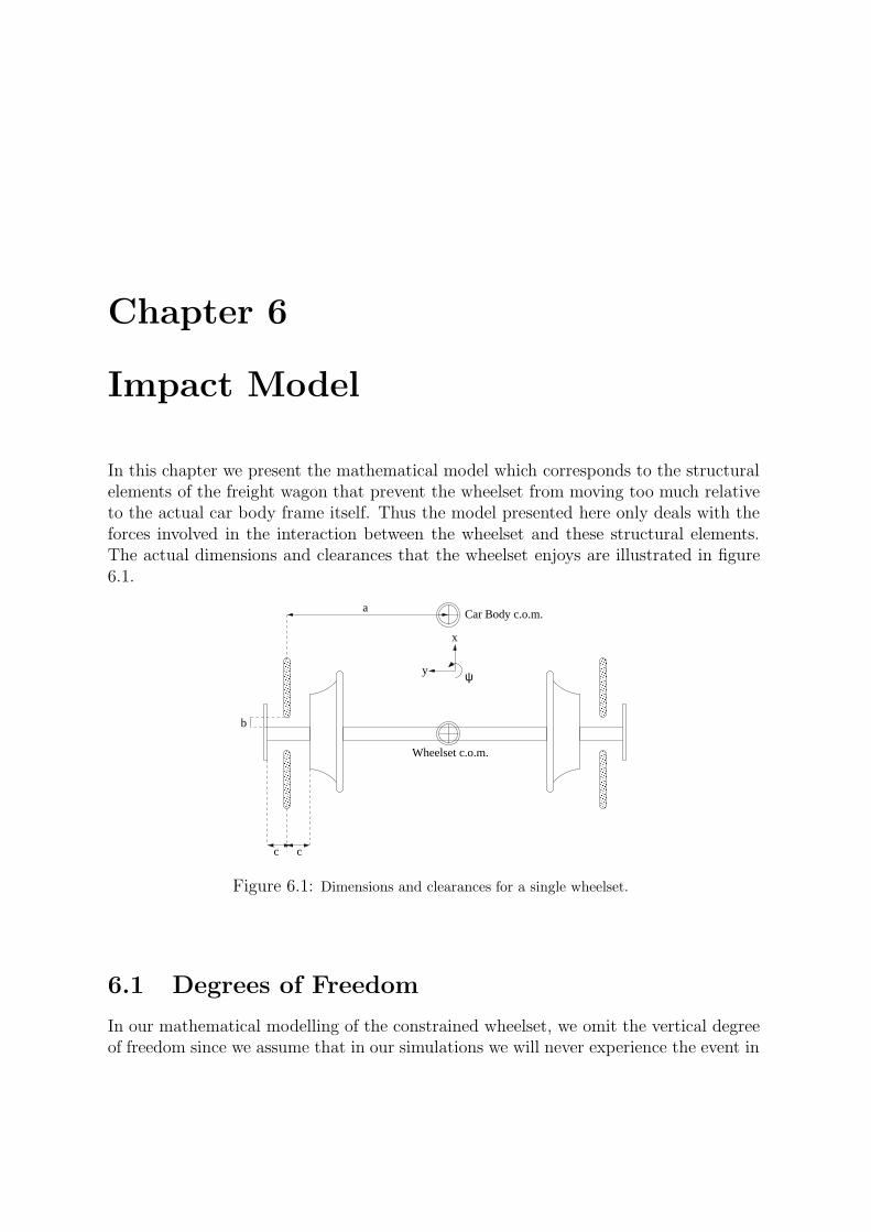
Chapter 6
Impact Model
In this chapter we present the mathematical model which corresponds to the structuralelements of the freight wagon that prevent the wheelset from moving too much relativeto the actual car body frame itself. Thus the model presented here only deals with theforces involved in the interaction between the wheelset and these structural elements.The actual dimensions and clearances that the wheelset enjoys are illustrated in figure6.1.
�������������
�������������
�������������
�������������
�������������
�������������
�������������
�������������
b
c c
a Car Body c.o.m.
Wheelset c.o.m.
y
x
ψ
Figure 6.1: Dimensions and clearances for a single wheelset.
6.1 Degrees of Freedom
In our mathematical modelling of the constrained wheelset, we omit the vertical degreeof freedom since we assume that in our simulations we will never experience the event in

64 Impact Model
which the leaf spring compresses to such a degree that the wheelset axle impacts withthe car body frame. Furthermore, wheelset pitch is inconsequential for the behaviourof our wheelset in this case. Wheelset roll is also considered to be too small to be ofimportance. Therefore we have the following degrees of freedom.
x : Wheelset longitudinal
y : Wheelset lateral
ψ : Wheelset yaw
6.2 Mathematical Model
Figures that illustrate the forces on our mathematical model are shown in figures 6.2and 6.3. From these figures we can determine the equations of motion for our system,based on Newton’s second law. The coordinate system for this model can be taken to be(Xr, Yr, Zr), the rail coordinate system. Keep in mind that the lateral and longitudinaldisplacements of the center of mass of the wheelset will be known as xd and yd in thischapter.
ba
1a
2a
y
x
ψ
1ττ2
Figure 6.2: Forces and dimensions concerning longitudinal impacts.
The values a1 and a2 are given by:
a1 =a+ ydcos(ψ)
a2 =a− ydcos(ψ)
6.2.1 Impact
The forces that arise from impact, τ , come from what we model as linear springs whichonly exert their restoring force once the wheelset comes into contact with the freight

6.2 Mathematical Model 65
ac c
ab
ψ
x
y
a
4τ 3τ
5τ
6τ5
a4a3
a6
Figure 6.3: Forces and dimensions concerning lateral impacts.
wagon structure. Furthermore, these forces are directed in parallel with the unit vectorsthat define the x and y coordinates in our mathematical model. These forces are alsoconsidered to exist in a plane parallel to the ground plane that the rails rest on.
Thus we need to know the longitudinal penetration of the wheelset that gives rise toforces τ1 and τ2. The positions of the penetrating wheelset points will be known as px,1and px,2, respectively, while actual penetration will be calculated later. The values px,1and px,2 are determined by:
px,1 = a1 sin(ψ) + xd
px,2 = −a2 sin(ψ) + xd
For τ3 through τ6 we will need to know the lateral penetration of the wheelset intothe local structure, and the corresponding wheelset penetrating positions will be knownas py,3 through py,6. The values py,3 to py,6 are determined by:
py,3 = −a3 cos(ψ) + yd
py,4 = −a4 cos(ψ) + yd
py,5 = a5 cos(ψ) + yd
py,6 = a6 cos(ψ) + yd
where a3 to a6 are the absolute distances from the center of mass of the wheelset to theimpact points.
a3 = a+ c
a4 = a− c
a5 = a− c
a6 = a+ c

66 Impact Model
6.2.2 Equations
The physical equations of motion of a wheelset restricted by guidances, are as follows:
mwx = τ1 + τ2
mwy = τ3 + τ4 + τ5 + τ6
Iwzψ = a1τ1 cos(ψ) − a2τ2 cos(ψ) + a3τ3 sin(ψ) + a4τ4 sin(ψ) − a5τ5 sin(ψ) − a6τ6 sin(ψ)
y1 = x
y2 = x
y3 = y
y4 = y
y5 = ψ
y6 = ψ
In order to achieve a system of first order ordinary differential equations, we differ-entiate the previous values, and obtain the following system.
y1 = y2
y2 =τ1 + τ2mw
y3 = y4
y4 =τ3 + τ4 + τ5 + τ6
mw
y5 = y6
y6 =a1τ1 cos(y5) − a2τ2 cos(y5) + a3τ3 sin(y5) + a4τ4 sin(y5) − a5τ5 sin(y5) − a6τ6 sin(y5)
Iwz
6.2.3 Forces
In order to determine the forces τ that arise under impact, we have following conditionalformulas where k represents a linear spring constant. Under actual simulation, the lateraland longitudinal stiffnesses will vary.
τ1 =
−k(px,1 + b) if px,1 < −b−k(px,1 − b) if px,1 > b
0 otherwise
τ2 =
−k(px,2 + b) if px,2 < −b−k(px,2 − b) if px,2 > b
0 otherwise
τ3 =
{ −k(py,3 + a) if py,3 > −a0 otherwise

6.3 Results 67
τ4 =
{ −k(py,4 + a) if py,4 < −a0 otherwise
τ5 =
{ −k(py,5 − a) if py,5 > a0 otherwise
τ6 =
{ −k(py,6 − a) if py,6 < a0 otherwise
6.3 Results
The system described in this chapter was modelled in MatLab (see impactode.m in thesource code). An interesting aspect of the introduction of the guidance constraints tothe wheelset is that it introduces nonlinearity that could lead to the presence of chaoticbehaviour in our freight wagon model. A characteristic property of chaotic systems isthat they exhibit sensitivity in the initial condition. In the following we will investigatewhether or not the impact model has this characteristic property. In table 6.1 wehave shown the parameters used in the first numerical example. The magnitude of bothclearances, i.e. b and c, are not realistic, however, they serve to exaggerate the sensitivityof the system for clarity.
Description Value
Wheelset mass 1022 kgWheelset yaw inertia 678 kg m2
Longitudinal guidance stiffness 1011 N m−1
Lateral guidance stiffness 1.5 · 106 N m−1
a 1.074 mb 0.5 mc 0.2 m
Table 6.1: Parameters used in the sensitivity test.
The numerical solution was found with the MatLab solver ode15s, with absolute andrelative tolerances of 10−8, and the following initial conditions:
Y0,1 = [0, 0.6, 0, 0.3, 0, 0]T (Unperturbed)
Y0,2 = Y0,1 +[0, 0, 10−6, 0, 0, 0
]T(Perturbed)
The result is presented in figure 6.4. It is seen that even though the solution start outin almost identical positions, the asymtotic solution is completely different.

68 Impact Model
The second numerical example is with the true clearance dimensions, i.e. b = 0.0225m and c = 0.02 m. We expect a similar result as in the first numerical example, however,there is a slightly difference as seen in figure 6.5. The sensitivity is clearly visible in thelongitudinal displacement as well as the yaw motion, but the lateral displacement isalmost the same even after a long time.

6.3 Results 69
0 5 10 15 20 25 30 35 40−0.5
−0.4
−0.3
−0.2
−0.1
0
0.1
0.2
0.3
0.4
0.5
Time [s]
Cen
ter
of M
ass
(long
itudi
nal d
ispl
acem
ent)
[m]
UnperturbedPerturbed
(a) Longitudinal.
0 5 10 15 20 25 30 35 40−0.25
−0.2
−0.15
−0.1
−0.05
0
0.05
0.1
0.15
0.2
0.25
Time [s]
Cen
ter
of M
ass
(late
ral d
ispl
acem
ent)
[m]
UnperturbedPerturbed
(b) Lateral.
0 5 10 15 20 25 30 35 40−0.4
−0.3
−0.2
−0.1
0
0.1
0.2
0.3
0.4
0.5
Time [s]
Yaw
ang
le [r
ad]
UnperturbedPerturbed
(c) Yaw.
−0.5 −0.4 −0.3 −0.2 −0.1 0 0.1 0.2 0.3 0.4 0.5−0.25
−0.2
−0.15
−0.1
−0.05
0
0.05
0.1
0.15
0.2
0.25
Longitudinal displacement of COM [m]
Late
ral d
ispl
acem
ent o
f CO
M [m
]
Unperturbed
(d) Trace of the center of mass inthe test with the unperturbed ini-tial condition.
−0.5 −0.4 −0.3 −0.2 −0.1 0 0.1 0.2 0.3 0.4 0.5−0.25
−0.2
−0.15
−0.1
−0.05
0
0.05
0.1
0.15
0.2
0.25
Longitudinal displacement of COM [m]
Late
ral d
ispl
acem
ent o
f CO
M [m
]
Perturbed
(e) Trace of the center of mass inthe test with the perturbed initialcondition.
Figure 6.4: Solution of the impact model with exaggerated clearances illustrating the sensitivity inthe initial condition.

70 Impact Model
0 20 40 60 80 100 120 140 160 180 200−0.025
−0.02
−0.015
−0.01
−0.005
0
0.005
0.01
0.015
0.02
0.025
Time [s]
Cen
ter
of M
ass
(long
itudi
nal d
ispl
acem
ent)
[m]
UnperturbedPerturbed
(a) Longitudinal.
0 20 40 60 80 100 120 140 160 180 200−0.025
−0.02
−0.015
−0.01
−0.005
0
0.005
0.01
0.015
0.02
0.025
Time [s]
Cen
ter
of M
ass
(late
ral d
ispl
acem
ent)
[m]
UnperturbedPerturbed
(b) Lateral.
0 20 40 60 80 100 120 140 160 180 200−0.025
−0.02
−0.015
−0.01
−0.005
0
0.005
0.01
0.015
0.02
0.025
Time [s]
Yaw
ang
le [r
ad]
UnperturbedPerturbed
(c) Yaw.
−0.025 −0.02 −0.015 −0.01 −0.005 0 0.005 0.01 0.015 0.02 0.025−0.025
−0.02
−0.015
−0.01
−0.005
0
0.005
0.01
0.015
0.02
0.025
Longitudinal displacement of COM [m]
Late
ral d
ispl
acem
ent o
f CO
M [m
]
Unperturbed
(d) Unperturbed.
−0.025 −0.02 −0.015 −0.01 −0.005 0 0.005 0.01 0.015 0.02 0.025−0.025
−0.02
−0.015
−0.01
−0.005
0
0.005
0.01
0.015
0.02
0.025
Longitudinal displacement of COM [m]
Late
ral d
ispl
acem
ent o
f CO
M [m
]
Perturbed
(e) Perturbed.
Figure 6.5: Solution of the impact model with true clearance dimensions, i.e. b = 0.0225 m andc = 0.02 m. The sensitivity in the initial condition is seen in the longitudinal displacement and yawmotion, however, the lateral displacement is more or less the same.

Chapter 7
Freight Wagon Inertia
This chapter deals with calculating the moments of inertia of the Hbbills 311 freightwagon, either empty or loaded. Since explicit data on the moments of inertia were notreadily available, these had to be calculated from a table detailing the elements on aHbbills 311 freight wagon.
7.1 Empty Freight Wagon
Table 7.1 details the quantity and mass of the different elements which we have consid-ered to be a significant part of the empty Hbbills 311 freight wagon.The center of mass is defined as
rC =1
M
∑i
miri (discrete)
rC =1
M
∫rρ dS =
1
A
∫r dS (continuous)
The moment of inertia is defined as
Iz =∑i
miR2i (discrete)
Iz =
∫R2ρ dS =
M
A
∫R2 dS (continuous)
where R is the distance to the z-axis.We use Maple to calculate both the center of mass as well as moments of inertia, and
the Maple code is given in appendix G. Results are the following:
rC = (x0, y0, z0) = (8.005 m, 1.450 m, 0.802 m)

72 Freight Wagon Inertia
and
Iroll = 32675 kg · m2
Iyaw = 413097 kg · m2
The coordinate system used is shown in figure 7.1. In this figure, Iroll and Iyaw are themoments of inertia with respect to the lines l1 and l2, respectively.
7.2 Adding Freight
In adding freight, we add a neat 20 tons to the wagon, and assume that the freight isevenly distributed over the floor. This means that the height of the freight measuredfrom the floor is
ρ =Mfreight
h · A ⇒ h =Mfreight
ρ · d8 · d9
< d4 ≈ 2.35 m
The center of mass of the car body is now placed at
rC =
(x0, y0,
z0M0 + (12h+ d3)Mfreight
M0 +Mfreight
)
where d3 ≈ 0.265 m is the distance from the underframe to the floor. We repeat thecalculations for Iroll and Iyaw with respect to the new center of mass of the car bodythrough the use of Steiner’s theorem.
In the dynamic simulations presented later in this report we have used four differenttypes of freight summarized in table 7.2 and 7.3. We have chosen these types in orderto be able to simulate what happens when the center of mass of the car body is raisedor lowered. Furthermore, we are interested in discussing the difference in the dynamicbehaviour between an empty wagon and a loaded wagon.

7.2 Adding Freight 73
Element # Mass [kg] (each) Mass [kg] (total)
Underframe 1 6395 6395Floor 1 662 662Front wall 2 550 1100Roof 1 1339 1339Partition 4 244 976Sliding panel 2 1024 2048Rail for sliding panel 2 132 264Buffer 4 149 596Center column 1 183 183
Sum - - 13563
Table 7.1: Quantities and masses of different significant elements of a Hbbills 311 freight wagon.
Freight Mass [kg] Density [kg/m3]
H2O 20000 1000.0Au 20000 19300.0
Packed 20000 183.3
Table 7.2: A few characteristics of chosen freight compositions.
Freight COM of car body with freight [m] Iroll [kg · m2] Iyaw [kg · m2]
Empty (8.005, 1.450, 0.802) 32675 413097H2O (8.005, 1.450, 0.610) 48428 854314Au (8.005, 1.450, 0.489) 49893 854314
Packed (8.005, 1.450, 1.182) 58014 854314
Table 7.3: Center of mass of the whole car body and freight, as well as moments of inertia for differentfreights.

74 Freight Wagon Inertia
d1 d2d1
d3
d4
d5
d6
y
z
d7
������������������
������������������
������������������
������������������
Partition
Floor
Underframe
Slid
ing
pane
ls
Slid
ing
pane
ls
Roof 1 Roof 2 Roof 3
Buffer Buffer
(a) Front view.
2 Partitions
Front wall
2 Partitions
Front wall
d 4
d 3
d 5
l 1
l 2
z
x
d 8
Roof
4 Sliding panels
Underframe
Floor
Rails
Cen
ter
colu
mn
(b) Side view.
d1
d2
d1
l 1
d
y
x
d8
7
d9
���������������
���������������
���������������
���������������
���������������
���������������
���������������
���������������
(c) Top view.
Figure 7.1: Model pictures used in the determination of the moments of inertia.

Chapter 8
Dry Friction Dynamics
In this section we will briefly look into the dynamics of the basic dry friction element thatis used as a model for the UIC link suspension in the lateral and longitudinal directions.The purpose of this is to get some insight in the properties of dry friction, because itmight not be that easy to extract this information when analyzing the complete model.
k1 T01
k
m
Figure 8.1: Dry friction model under investigation.
We consider a mass connected to a fixed base through the dry friction element (seefigure 8.1). This element is comprised of a main spring, with stiffness k, and a secondaryspring attached to a dry friction slider. This dry friction slider is central to the dynamicsof the element, in that it changes the whole stiffness of the system, depending on wetheror not the slider sticks, or is slipping. When sticking, the stiffness of the element is k+k1,and when sliding, only the main spring is left to govern dynamics, and the stiffness isonly k.
The dry friction slider can be visualized as two plates pressed against each other,of which can maximally sustain a shearing force equal to T0 before static friction isovercome and the slider begins to slip. Important to note is that in our model here,and in the freight train itself, we do not distinguish between static and kinetic frictioncoefficients (figure F.2(a) in appendix validates this assumption). This results in thatwhen sliding, the slider element delivers a maximum force T0.
A numerical experiment is performed as follows. For t < 0 the mass is at rest, allspring forces are zero, no shear force exists in the slider, and this position defines the

76 Dry Friction Dynamics
“true” origin of our coordinate system. At t = 0 we pull out the mass to the position x0
and release.The time history of the simulation is shown in figure 8.2. In the first part of the figure
we see damped oscillations. What is characteristic of systems exhibiting dry friction, isthat the envelope of the damping motion is linear, and not exponentially decaying, forexample.
After a while this damping ceases and the mass oscillates harmonically. This resultis not surprising, because the restoring force of the spring connected to the dry frictionslider is limited by a threshold force corresponding to the static coefficient of friction.The initial condition is so large that this limit is exceeded, meaning that the dry frictionplates begins to slide. As soon as the mass reaches a velocity of 0, the relative velocityin the dry friction slider also reaches 0, and the sliders stick immediately. This stickremains until the displacement of the mass becomes great enough that the force yieldedfrom the spring with stiffness k1 yet again overcomes the static friction threshold of theslider. This repeated sliding/sticking process yields a damping effect.
Ultimately, when the oscillations are damped to a certain magnitude the dry frictionplates will stick permanently since the shear force exerted on the dry friction plates nolonger exceeds the threshold mentioned above. At that point, the motion of the masswill appear as pure harmonic motion.
An interesting observation is that this harmonic motion need not necessarily oscillatesymetrically about the origin. This is evident in figure 8.4. This is because that fromthe system’s true origin, where all spring forces are zero, a band exists about this valuewhere the system can behave as having a new origin upon reaching harmonic motion.This is because as the slider slips when forces exceed its threshold, the origin for theslider spring (stiffness k1) moves. This movement results in a bit of force coming fromthe slider spring, where before it was 0 at the system’s true origin, it now no longer isso, and thus shifts the center point of oscillation of the collected system.
This behaviour is confirmed in our mathematical model in figure 8.4, as well as inexperimental data from Poland. It was previously mentioned how we zero-shifted data inorder to more accurately ascertain parameters for the UIC suspension. This behaviour,as we shall see, also emerges in the simulation of the full freight wagon.
An interesting figure of the dynamics of the simple dry friction model is given infigure 8.5. We here see a three dimensional trace of the state of our model. This traceis shown as a time history in figure 8.2, and a hysteresis loop diagram in figure 8.3. Wecan clearly see the dry friction force is limited by T0, since the force plateaus under toogreat displacement. The figure gives a good overview of the dry friction force as ourmass moves from damped motion to harmonic motion.

77
0 5 10 15 20 25 30 35 40 45 50−0.5
−0.4
−0.3
−0.2
−0.1
0
0.1
0.2
0.3
0.4
0.5
Time [s]
Dis
plac
emen
t [m
]
Time series of the displacement
Figure 8.2: Time history for the experiment showing the damping effect of the dry friction.
−0.5 −0.4 −0.3 −0.2 −0.1 0 0.1 0.2 0.3 0.4 0.5−2
−1.5
−1
−0.5
0
0.5
1
1.5
2
Displacement [m]
For
ce [N
]
Hysteresis loop of the restoring force
Figure 8.3: Complete hysteresis loop of the experiment.

78 Dry Friction Dynamics
−0.03 −0.02 −0.01 0 0.01 0.02 0.03 0.04
−0.4
−0.2
0
0.2
0.4
0.6
Displacement [m]
For
ce [N
]
Hysteresis loop of the restoring force
Figure 8.4: Zoomed view of the hysteresis loop. The oscillations is clearly not around zero.
−0.5
0
0.5−1
−0.5
0
0.5
1
−0.1
−0.05
0
0.05
0.1
Velocity [m/s]Displacement [m]
Slid
er F
orce
[N]
Figure 8.5: This figure shows the dry friction force as a function of the displacement and velocityof the mass. By imagining the slider force versus velocity projection one can see the Coulomb frictionrelationship between the friction force and sliding velocity. Furthermore, this figure gives an illustrationof damping that the mass is exposed to each time dry friction plates slides.

Chapter 9
Numerical Approach
9.1 Implementation
The implementation is done in C++ for three reasons. First, executing programs inC++ can be done efficiently compared to other programming languages such as MatLaband Java. Secondly, C++ allow object oriented programming yielding a better programstructure. Thirdly, the numerical solver we were provided with is also programmedin C++, and thus applying the solver to our model is straight forward. The completeprogram is found in the source code supplement to this thesis.
The model is“built” in the file FreightWagon.cpp and is a composition of six objects.These objects are created through six C++ classes also listed in the source code. A shortdescription of the classes are now given.
• CarBody. Implementation of the car body model. This object delivers the dif-ferential equations regarding the car body given the magnitude of the suspensionand impact forces.
• Impact. Implementation of the impact model. Through the interface of thisobject we compute the impact forces given the current position of the wheelsetsand the car body.
• Parameters. Object through which it is possible to read in parameters from datafiles.
• Suspension. Implementation of the linear, parabolic and leaf spring model.Through the interface of this object we compute the suspension forces given thecurrent position of the wheelsets and the car body.
• WheelRailContact. Implementation of the wheel-rail contact model. Throughthe interface of this object we compute the contact forces between the wheel andrail for one of the wheelsets given the current position of the specific wheelset.
80 Numerical Approach
• Wheelset. Implementation of the wheelset model. This object delivers the dif-ferential equations regarding the wheelset given the magnitude of the suspension,impact and contact forces.
9.2 SDIRK
In the treatment of our problem, we employed the numerical solver SDIRK, as providedby prof. Per Grove Thomsen1. This solver was employed by [11] and partially by [4].SDIRK belongs to the Runge-Kutta family of solvers, and more precisely, the singlydiagonally implicit Runge-Kutta solvers (which is the origin of the acronym SDIRK).As such, it is an efficient solver for stiff problems, and requires the specification of theJacobi matrix of our system, as well as the right hand side of our system of first orderODEs.
9.3 Jacobi Matrix
Since we have to calculate the Jacobi matrix of the complete system, we investigate thisstep here. It is very important from an efficiency point of view to optimize the calcula-tion of the Jacobi matrix in order to minimize computer time during simulations. Thereason calculation of the Jacobi matrix is time consuming is that in each integrationstep the numerical integrator requires several approximations of the system in orderto approximate the next solution point. In that the Jacobi matrix has numerous el-emenets, multiple calculations of its elements for every time step translates into a heavycomputational load.
The definition of the (i, j)’th element in the Jacobi matrix is
Jij =∂fi∂yj
(9.1)
Some of the elements we have to evaluate numerically because the forces govering themotion of the vehicle are determined by non analytic functions. A naıve and extremelyinefficient method is to go through all elements in the Jacobi matrix and numericallyestimate the derivative. This is inefficient because the Jacobi matrix is a sparse matrix,meaning that most of the entries are zero. In figures 9.1(a), 9.1(b) and 9.1(c) we haveillustrated the sparsity pattern of the Jacobi matrix for our system using suspensiontypes 1, 2 and 3, respectively. However, to find the nonzero entries we have to lookinto the dependencies in each equation in the complete system for the correspondingsuspension type. In section 9.4 these dependencies are listed.
1Institute for Informatics and Mathematical Modelling, Technical University of Denmark.

9.3 Jacobi Matrix 81
By knowing the dependecies we can efficiently evaluate the Jacobi matrix in thefollowing manner. We characterise each element in the Jacobi matrix by how the valueof the element is provided. We distinguish between the entries that are zero, one andthose we have to approximate numerically. This characterization is done before thesimulation starts, meaning that the only time consuming part in the determination ofthe Jacobi matrix under the simulation is the special entries that we need to approximatenumerically, which only form a minor part of the complete matrix.
The numerical approximation to the derivative in equation (9.1) is done by a centraldifference estimate. To make this estimate we calculate the function value of fi for apositive and negative perturbation of the variable yj . The central difference is thenformed by
∂fi∂yj
≈ fi,+ − fi,−2δ
(9.2)
where δ is the perturbation.To make this numerical approximation procedure efficient, with respect to processing
time, we proceed columnwise2 through the Jacobi matrix and follow the scheme:
1. Perturb yj positively by δ
2. Calculate the interacting forces
3. Calculate and store all fi,+
4. Perturb yj negatively by δ
5. Calculate the interacting forces
6. Calculate and store all fi,−
7. Calculate the central difference by equation (9.2)
This is advantageous because we only have to determine the interacting forces betweenthe elements in the freight wagon twice for each yj.
A consequence of our central differences strategy is that elements are perturbed witha constant value throughout simulation. Since scale between Jacobi matrix elementsdiffer greatly, we optimized roughly the perturbation magnitude with respect to whatJacobi matrix element we were estimating, but this magnitude remained unchangedwith time. Since the scale of Jacobi elements change with respect to themselves overtime, poor estimation of certain elements can happen, with the result of the simulationhanging. A desirable strategy would be a Jacobi matrix estimator that optimizes themagnitude of pertubation, much like numjac can do for MatLab implemented systems.
2Programming language specific optimization. Fortran would be optimized to proceed row by row.

82 Numerical Approach
This may have enabled us to simulate without much user intervention to overcome hungsimulations. Ultimately, we did not have the time to experiment and develop such anefficient numerical Jacobi matrix estimator.
0 5 10 15 20 25 30
0
5
10
15
20
25
30
nz = 268
Suspension Type 1
(a) Suspension type 1. 30× 30.
0 5 10 15 20 25 30 35 40 45 50
0
5
10
15
20
25
30
35
40
45
50
nz = 401
Suspension Type 2
(b) Suspension type 2. 50× 50.
0 5 10 15 20 25 30 35 40 45 50 55
0
5
10
15
20
25
30
35
40
45
50
55
nz = 409
Suspension Type 3
(c) Suspension type 3. 54 × 54.
Figure 9.1: Non-zero elements for Jacobi matrices using suspension types (a) 1, (b) 2, and (c) 3.

9.4 Dependencies 83
9.4 Dependencies
9.4.1 Front Wheelset
The calculation of the contact forces
Crlx, C
rrx, C
rly, C
rry, C
rlz, C
rrz, C
wlx, C
wrx, C
wly, C
wry, C
wlz , C
wrz
is a function off(y2, y3, y4, y5, y6, y7, y8, y9, y10, y11)
We write this dependency as follows∣∣∣∣ Crlx, C
rrx, C
rly , C
rry, C
rlz , C
rrz, C
wlx, C
wrx, C
wly , C
wry, C
wlz , C
wrz
f(y2→11)
Furthermore, we have∣∣∣∣∣∣∣∣Sr
lx, Srrx
f(y1, y2, y10, y11, y29, y30) Suspension type 1f(y1, y10, y29, y31→38) Suspension type 2f(y1, y10, y29, y31→38) Suspension type 3∣∣∣∣∣∣∣∣Sr
ly, Srry
f(y3, y4, y23, y24, y27→30) Suspension type 1f(y3, y23, y27, y29, y47, y48) Suspension type 2f(y3, y23, y27, y29, y47, y48) Suspension type 3∣∣∣∣∣∣∣∣Sr
lz , Srrz
f(y5→8, y25→28) Suspension type 1f(y5→8, y25→28) Suspension type 2f(y51, y52) Suspension type 3∣∣∣∣∣∣∣∣Sw
lx, Swrx
f(y1→4, y10, y11, y23, y24, y27→30) Suspension type 1f(y1, y3, y10, y23, y27, y29, y31→38, y47, y48) Suspension type 2f(y1, y3, y10, y23, y27, y29, y31→38, y47, y48) Suspension type 3∣∣∣∣∣∣∣∣Sw
ly, Swry
f(y1→8, y10, y11, y23→30) Suspension type 1f(y1, y3, y5→8, y10, y23, y25→29, y31→38, y47, y48) Suspension type 2f(y1, y3, y7, y10, y23, y27, y29, y31→38, y47, y48, y51, y52) Suspension type 3∣∣∣∣∣∣∣∣Sw
lz , Swrz
f(y3→8, y23→30) Suspension type 1f(y3, y5→8, y23, y25→29, y47, y48) Suspension type 2f(y3, y7, y23, y27, y29, y47, y48, y51, y52) Suspension type 3
∣∣∣∣ δrlx, δ
rrx
f(y1, y10, y29)
∣∣∣∣ δrly, δ
rry
f(y3, y23, y27, y29)
∣∣∣∣ δrlz , δ
rrz
0∣∣∣∣ δwlx, δ
wrx
f(y1, y3, y10, y23, y27, y29)
∣∣∣∣ δwly, δ
wry
f(y1, y3, y7, y10, y23, y27, y29)
∣∣∣∣ δwlz , δ
wrz
f(y3, y7, y23, y27, y29)

84 Numerical Approach
9.4.2 Rear Wheelset
For the rear wheelset we have the following dependencies.
∣∣∣∣ Crlx, C
rrx, C
rly, C
rry, C
rlz , C
rrz, C
wlx, C
wrx, C
wly, C
wry, C
wlz , C
wrz
f(y13→22)∣∣∣∣∣∣∣∣Sr
lx, Srrx
f(y12, y13, y21, y22, y29, y30) Suspension type 1f(y12, y21, y29, y39→46) Suspension type 2f(y12, y21, y29, y39→46) Suspension type 3∣∣∣∣∣∣∣∣Sr
ly , Srry
f(y14, y15, y23, y24, y27→30) Suspension type 1f(y14, y23, y27, y29, y49, y50) Suspension type 2f(y14, y23, y27, y29, y49, y50) Suspension type 3∣∣∣∣∣∣∣∣Sr
lz , Srrz
f(y16→19, y25→28) Suspension type 1f(y16→19, y25→28) Suspension type 2f(y53, y54) Suspension type 3∣∣∣∣∣∣∣∣Sw
lx, Swrx
f(y12→15, y21→24, y27→30) Suspension type 1f(y12, y14, y21, y23, y27, y29, y39→46, y49, y50) Suspension type 2f(y12, y14, y21, y23, y27, y29, y39→46, y49, y50) Suspension type 3∣∣∣∣∣∣∣∣Sw
ly , Swry
f(y12→19, y21→30) Suspension type 1f(y12, y14, y16→19, y21, y23, y25→29, y39→46, y49, y50) Suspension type 2f(y12, y14, y18, y21, y23, y27, y29, y39→46, y49, y50, y53, y54) Suspension type 3∣∣∣∣∣∣∣∣Sw
lz , Swrz
f(y14→19, y23→30) Suspension type 1f(y14, y16→19, y23, y25→29, y49, y50) Suspension type 2f(y14, y18, y23, y27, y29, y49, y50, y53, y54) Suspension type 3
∣∣∣∣ δrlx, δ
rrx
f(y12, y21, y29)
∣∣∣∣ δrly , δ
rry
f(y14, y23, y27, y29)
∣∣∣∣ δrlz, δ
rrz
0
∣∣∣∣ δwlx, δ
wrx
f(y12, y14, y21, y23, y27, y29)
∣∣∣∣ δwly , δ
wry
f(y12, y14, y18, y21, y23, y27, y29)
∣∣∣∣ δwlz, δ
wrz
f(y14, y18, y23, y27, y29)
9.4.3 Car Body
For the car body the dependencies are found to be

9.4 Dependencies 85
∣∣∣∣∣∣∣∣Sr
flx, Srfrx, S
rrlx, S
rrrx
f(y1, y2, y10→13, y21, y22, y29, y30) Suspension type 1f(y1, y10, y12, y21, y29, y31→46) Suspension type 2f(y1, y10, y12, y21, y29, y31→46) Suspension type 3∣∣∣∣∣∣∣∣Sr
fly, Srfry, S
rrly, S
rrry
f(y3, y4, y14, y15, y23, y24, y27→30) Suspension type 1f(y3, y14, y23, y27, y29, y47→50) Suspension type 2f(y3, y14, y23, y27, y29, y47→50) Suspension type 3∣∣∣∣∣∣∣∣Sr
flz, Srfrz, S
rrlz, S
rrrz
f(y5→8, y16→19, y25→28) Suspension type 1f(y5→8, y16→19, y25→28) Suspension type 2f(y51→54) Suspension type 3∣∣∣∣∣∣∣∣Sb
flx, Sbfrx, S
brlx, S
brrx
f(y1→4, y10→15, y21→24, y27→30 Suspension type 1f(y1, y3, y10, y12, y14, y21, y23, y27, y29, y31→50) Suspension type 2f(y1, y3, y10, y12, y14, y21, y23, y27, y29, y31→50) Suspension type 3∣∣∣∣∣∣∣∣Sb
fly, Sbfry, S
brly, S
brry
f(y1→8, y10→19, y21→30) Suspension type 1f(y1, y3, y5→8, y10, y12, y14, y16→19, y21, y23, y25→29, y31→50) Suspension type 2f(y1, y3, y10, y12, y14, y21, y23, y27, y29, y31→54) Suspension type 3∣∣∣∣∣∣∣∣Sb
flz, Sbfrz, S
brlz, S
brrz
f(y3→8, y14→19, y23→30) Suspension type 1f(y3, y5→8, y14, y16→19, y23, y25→29, y47→50) Suspension type 2f(y3, y14, y23, y27, y29, y47→54) Suspension type 3
∣∣∣∣ δrflx, δ
rfrx, δ
rrlx, δ
rrrx
f(y1, y10, y12, y21, y29)
∣∣∣∣ δrfly, δ
rfry, δ
rrly, δ
rrry
f(y3, y14, y23, y27, y29)∣∣∣∣ δrflz , δ
rfrz, δ
rrlz, δ
rrrz
0
∣∣∣∣ δbflx, δ
bfrx, δ
brlx, δ
brrx
f(y1, y3, y10, y12, y14, y21, y23, y27, y29)∣∣∣∣ δbfly, δ
bfry, δ
brly, δ
brry
f(y1, y3, y10, y12, y14, y21, y23, y27, y29)
∣∣∣∣ δbflz, δ
bfrz, δ
brlz, δ
brrz
f(y3, y14, y23, y27, y29)
9.4.4 Dry Friction Elements
yi = f(y2, y11, y30, yi) i = 31 . . .38yi = f(y13, y22, y30, yi) i = 39 . . .46yi = f(y4, y24, y28, y30, yi) i = 47, 48yi = f(y15, y24, y28, y30, yi) i = 49, 50yi = f(y5→8, y25→28, yi) i = 51, 52yi = f(y16→19, y25→28, yi) i = 53, 54

86 Numerical Approach

Chapter 10
Results
10.1 Method of Attack
In this chapter we present results from various simulations on our freight wagon underdifferent conditions. This encompasses both suspension parameter sets, as well as differ-ent cargo conditions. The suspension setup in all cases was the model for the UIC linksin longitudinal and lateral direction, whereas the parabolic spring model was used in thevertical direction. Fancher’s model describing standard leaf springs was simulated, butwe did not produce any meaningful results in that the extreme stiffness of the systemlengthened simulation execution times significantly. The results were generated with theSDIRK solver using the SC_PI1 step control option, as well as a maximal error toleranceof 10−6.
We have generated bifurcation traces using the following algorithm:
1. Find stationary solution at a certain velocity v.
2. Simulate 5 or 10 seconds running at v.
3. Capture maximum amplitude over the last 3 seconds.
4. v = v ± 0.05 m/s and goto 2.
We have used the bifurcation diagrams as a starting point for further analysis of themodel. Thus, we first present bifurcation diagrams followed by specific simulationsdigesting the information from the diagrams. This is done for both suspension parametersets. Finally, we do a frequency analysis capturing the main frequencies in the model.
1SC_PI is short for Proportional-Integral step control.

88 Results
10.2 Suspension Parameter Set 1
10.2.1 Critical Velocities
In figure 10.1(a) we show a bifurcation trace performed on an empty freight wagon.We started at 15 m/s with all elements being in centered position. Since we are underthe linear critical velocity the equilibrium in the center of track is stable and thus theelements remain in centered position. By increasing the velocity slowly we moved from15 m/s up to 23 m/s, and we observe that the stable equilibrium in the center of thetrack has turned into an unstable equilibrium, which indicates that we have passed thelinear critical velocity. This happens around 20 m/s, and from our knowledge fromrailway dynamics this bifurcation is expected to be a subcritical Hopf bifurcation, atwhat is known as the linear critical velocity. That it is truly a Hopf bifurcation is seenin the eigenvalue analysis shown in figure 10.2. This figure shows how the eigenvaluesmigrate for velocities around v = 18.4 m/s. One interesting thing about this migrationis that there exists two eigenvalues, which are complex conjugates of each other, thatcross the imaginary axis (see figure 10.2(c)), and thus we can be certain that a Hopfbifurcation takes place. Another interesting aspect to comment is that the bifurcationtrace analysis hinted at us that the Hopf bifurcation is about 20 m/s, but this is incontrast to the correct eigenvalue analysis that clearly shows that the Hopf bifurcationis at v = 18.4 m/s.
The problem is our criteria for judging a solution to have reached its asymptoticbehaviour. In principle one should simulate infintely long, but in practice this is notpossible, so we have to stop the simulation at a certain point. The consequence of doingthis is that we might not have reached the asymptotic solution, which is the situation inthe bifurcation trace at 18.5 m/s, for example. This is also illustrated in figure 10.2(d).We see that the equilibrium in the center of the track has a repelling tendency after theHopf bifurcation.
To determine the type of the Hopf bifurcation we investigated what happens rightafter the Hopf bifurcation. In contrast to our expectations we found that the Hopf bifur-cation actually is supercritical. This is based in that there exists a stable growing limitcycle after the bifurcation. The limit cycle is found by doing simulations at velocitiesjust above v = 18.4 m/s with initial conditions at the center of the track. The resultis that the solution after a while is repelled to the limit cycle (see figure 10.3(a) and10.3(b)).
However, by increasing the velocity further, this limit cycle is destroyed in a saddlenode bifurcation at around v = 18.6 m/s. Simulating at v = 18.7 m/s we found the resultin figure 10.3(c) and 10.3(d). This figure convinced us that the limit cycle is destroyedin a saddle node bifurcation, because what the figures show is a bottleneck effect typicalfrom the ghost right after a saddle node bifurcation. The solution trajectory finallyescapes the bottleneck and ends up on the hunting attractor found in the bifurcation

10.2 Suspension Parameter Set 1 89
diagram in figure 10.1(a). After this analysis we were convinced that the true bifurcationdiagram must exhibit a double saddle node bifurcation something like the diagram shownin figure 10.1(b), where the ghost we encountered is the one on the right.
One could argue that we have to increase our simulation time in the bifurcation tracesimulation. However, the amount of simulation time needed in order to get repelled fromthe centered position of the track is surprisingly large (see for example figure 10.3(a)).Thus, in order to be able to make the bifurcation diagrams at all (due to its extremelytime consuming process) we have used simulation times between 5 and 10 seconds, butwe have to be aware that it introduces at certain amount of delay.
From 23 m/s, we then slowly decellerated to 8 m/s and observed that the huntingmotion exists even for velocities under the critical value at v = 18.4 m/s. Thus thesystem exibits hysteresis. The hunting motion eventually disappears when the velocitybecomes less than another critical velocity known as the nonlinear critical velocity. Thishappens in a saddle node bifurcation about 9 m/s. The delay problem also occurs inthe determination of the nonlinear critical velocity, but only in the sense of the ghostattractor as previously discussed.
This same method was applied to the water loaded and packed freight wagon, andwe achieved the bifurcation traces in figures 10.1(c) and 10.1(d). Regarding the waterloaded wagon we estimated the linear critical velocity to be under 23 m/s, and thenonlinear critical velocity was found to be just over 9 m/s. For the packed freight wagonwe see a qualitatively changed bifurcation diagram in that the hunting attractor simplydisappears at about v = 17 m/s (at least we were not able to follow any attractordifferent from zero for velocities lower than v = 17 m/s). The linear critical velocity inthis case were about v = 25 m/s.
An immediate effect we can see in adding freight to the wagon is a stabilizing one.The Hopf bifurcation defining the linear critical velocity is raised by approximately 3m/s and 5 m/s, however, the nonlinear critical velocity is about the same in the waterloaded wagon case as for an empty wagon.
The bifurcation diagrams reveal an interesting conclusion on the dynamics of thefreight wagon, namely, that the worst dynamic behaviour is actually present at mediumvelocities, since the hunting attractor has a tendency to increase in amplitude towardsthe nonlinear critical velocity. Furthermore, we see a sharp discontinuity in the bifu-raction trace for the empty wagon at about 14 m/s, and for the water loaded wagonat 19 m/s. In these transition windows the motion did not reach any fixed amplitudeoscillation and thus many different amplitudes are present in the bifurcation diagram.This is illustrated in figure 10.4(a) and 10.4(b). These figures show a simulation withthe water loaded wagon running at v = 18.85 m/s. The conclusion from the figures isthat the chaotic looking discontinuities in the bifurcation diagrams actually is periodicwith the period of approximately 25 seconds.
The origin of these discontinuities is investigated in the subsection to come.

90 Results
8 10 12 14 16 18 20 22 240
0.005
0.01
0.015
0.02
0.025
0.03
Velocity [m/s]
Max
. lat
eral
dis
plac
emen
t [m
]
Bifurcation Diagram for Parameter Set 1
Front wheelsetRear wheelsetCar body
(a)
Amplitude
linear criticalVelocity
non−linear critical
GHOST
GHOST
(b)
8 10 12 14 16 18 20 22 24 260
0.005
0.01
0.015
0.02
0.025
0.03
0.035
0.04
0.045
Velocity [m/s]
Max
. lat
eral
dis
plac
emen
t [m
]
Bifurcation Diagram for Parameter Set 1
Front wheelsetRear wheelsetCar body
(c)
5 10 15 20 25 300
0.005
0.01
0.015
0.02
0.025
Velocity [m/s]
Max
. lat
eral
dis
plac
emen
t [m
]
Bifurcation Diagram for Parameter Set 1
Front wheelsetRear wheelsetCar body
(d)
Figure 10.1: (a) Bifurcation diagram for the empty freight wagon. (b) Schematic of how two saddlenode bifuractions for one of the elements may lie in our system. (c) Bifurcation diagram for the waterloaded freight wagon. (d) Bifurcation diagram for the packed freight wagon.

10.2 Suspension Parameter Set 1 91
−3500 −3000 −2500 −2000 −1500 −1000 −500 0 500−2000
−1500
−1000
−500
0
500
1000
1500
2000
Real axis
Imag
inar
y ax
is
Eigenvalue Migration
(a)
−1.2 −1 −0.8 −0.6 −0.4 −0.2 0 0.2 0.4 0.6
−10
−5
0
5
10
Real axis
Imag
inar
y ax
is
Eigenvalue Migration
(b)
−0.1 −0.05 0 0.05 0.1
−8
−6
−4
−2
0
2
4
6
8
10
Real axis
Imag
inar
y ax
is
Eigenvalue Migration
v = 18 m/s v = 19 m/s
(c)
18 18.2 18.4 18.6 18.8 19 19.2
6.66
6.665
6.67
6.675
6.68
6.685
6.69
x 10−9
Velocity [m/s]
Max
. lat
eral
dis
plac
emen
t [m
]
Bifurcation Diagram for Parameter Set 1
Front wheelsetRear wheelsetCar body
(d)
Figure 10.2: (a) All eigenvalues. (b) Zoomed view. The eigenvalue migration is clearly visible. (c)Zoomed view illustrating the Hopf bifurcation at v = 18.4 m/s. (d) delay effect.

92 Results
0 100 200 300 400 500 600 700 800 900 1000−3
−2
−1
0
1
2
3x 10
−3
Time [s]
Dis
plac
emen
t [m
]
Lateral Displacements
Front WheelsetRear WheelsetCar Body
(a) v = 18.5 m/s.
990 990.5 991 991.5 992 992.5 993 993.5 994 994.5 995−3
−2
−1
0
1
2
3x 10
−3
Time [s]
Dis
plac
emen
t [m
]
Lateral Displacements
Front WheelsetRear WheelsetCar Body
(b) v = 18.5 m/s zoomed.
0 50 100 150 200 250 300 350 400 450−0.02
−0.015
−0.01
−0.005
0
0.005
0.01
0.015
0.02
Time [s]
Dis
plac
emen
t [m
]
Lateral Displacements
Front WheelsetRear WheelsetCar Body
(c) v = 18.7 m/s.
440 441 442 443 444 445 446 447 448 449 450−0.02
−0.015
−0.01
−0.005
0
0.005
0.01
0.015
0.02
Time [s]
Dis
plac
emen
t [m
]
Lateral Displacements
Front WheelsetRear WheelsetCar Body
(d) v = 18.7 m/s zoomed.
Figure 10.3: Simulation of the empty wagon with the initial condition in the center of the track. Theanalysis shows that the Hopf-bifurcation is supercritical followed by a saddle node bifurcation. Theghost from the saddle node bifurcation causes the bottleneck effect seen in figure (c).

10.2 Suspension Parameter Set 1 93
0 10 20 30 40 50 60 70 80 90−0.04
−0.03
−0.02
−0.01
0
0.01
0.02
0.03
0.04
Time [s]
Dis
plac
emen
t [m
]
Lateral Displacements
Front WheelsetRear WheelsetCar Body
(a) Lateral motion in the ‘strange’ region of thewater loaded bifurcation diagram. v = 18.85 m/s.
40 45 50 55 60 65 70
−8
−6
−4
−2
0
2
4
6
8
x 10−3
Time [s]
Dis
plac
emen
t [m
]
Lateral Displacements
Front WheelsetRear Wheelset
(b) A zoomed view, illustrating lateral motionof the wheelsets showing a period of about 25seconds. v = 18.85 m/s.
Figure 10.4: These figures illustrate the periodic nature of the solutions in the ‘strange’ region(v = 18.85 m/s) of the water loaded bifurcation diagram. The bifurcation diagram has a strange regionas a consequence of the 3 second sampling time, and in this region, solutions oscillate with longerperiods.

94 Results
10.2.2 Guidance Impact Behaviour
We here present a series of figures which will serve to illustrate the effect of the wheelsetguidance structures. At first, we disable the guidance structures, and simulate the freightwagon, pretending that no wheelset guidance exists. Figures 10.5(a) and 10.5(b) showthe stable hunting behaviour that the freight wagon experiences at 25 m/s. However,as we lower the velocity, the periodic lateral hunting motion increases in amplitude, asdiscussed previously, and this is evident in figure 10.5(c) and 10.5(d) where we see thehunting motion grow at 20 m/s. Furthermore, at this speed, the wheelsets will actuallybegin to lose contact with the rails! This is why the simulation goes no further than itdoes.
When we enable the wheelset guidances, at 20 m/s, we see that the hunting amplitudeno longer seems to grow unbounded, but actually achieves a stable amplitude of about4 mm lateral movement for both wheelsets. This is illustrated in figures 10.5(e) and10.5(e). This simulation is also supported by figure 10.6 in which we show an impactanalysis. The top four figures show time histories of the impact forces in longitudinal andlateral direction on both wheelsets. The bottom two figures show the relative distancesto the guidances. It is seen that only the rear wheelset impacts laterally.
By simulating the empty wagon at v = 40 m/s with guidances we achieved the resultsin figure 10.7. Due to the contraction of the hunting attractor we do not see any impactin this case.
We now examine more closely some strange looking phenomena, observed in thebifurcation diagrams generated earlier. The bifurcation diagram for the empty wagonhas what seems to be two interesting discontinuities. The first interesting transitionpoint occurs at around 10 m/s, and the second one at just under 14 m/s. Regarding thebifurcation diagram for the water loaded wagon we saw a discontinuity at about v = 19m/s, and finally for the packed wagon we saw some strange behaviour at about v = 17m/s.
A series of results is presented for this investigation, and which are laid out in in therest of this section. These results illustrate time series for the motion of the wheelsetsand car body, as well as the impact characteristics of the wheelsets. For the emptywagon we show simulations at v = 15 m/s, v = 13 m/s, v = 11 m/s and v = 9.5 m/s, inthat order. This is followed by simulating the water loaded wagon at v = 20 m/s andv = 18 m/s. Finally, we have the packed wagon running at v = 17 m/s.

10.2 Suspension Parameter Set 1 95
0 5 10 15 20 25 30 35 40−3
−2
−1
0
1
2
3
4x 10
−4
Time [s]
Dis
plac
emen
t [m
]
Longitudinal Displacements
Front WheelsetRear Wheelset
(a) Longitudinal, v = 25 m/s.
0 5 10 15 20 25 30 35 40−0.015
−0.01
−0.005
0
0.005
0.01
0.015
Time [s]
Dis
plac
emen
t [m
]
Lateral Displacements
Front WheelsetRear WheelsetCar Body
(b) Lateral, v = 25 m/s.
0 5 10 15 20 25 30−2
−1.5
−1
−0.5
0
0.5
1
1.5
2x 10
−3
Time [s]
Dis
plac
emen
t [m
]
Longitudinal Displacements
Front WheelsetRear Wheelset
(c) Longitudinal, v = 20 m/s.
0 5 10 15 20 25 30−0.025
−0.02
−0.015
−0.01
−0.005
0
0.005
0.01
0.015
0.02
0.025
Time [s]
Dis
plac
emen
t [m
]
Lateral Displacements
Front WheelsetRear WheelsetCar Body
(d) Lateral, v = 20 m/s.
0 5 10 15 20 25 30−3
−2
−1
0
1
2
3
4x 10
−4
Time [s]
Dis
plac
emen
t [m
]
Longitudinal Displacements
Front WheelsetRear Wheelset
(e) Longitudinal, v = 20 m/s.
0 5 10 15 20 25 30−0.02
−0.015
−0.01
−0.005
0
0.005
0.01
0.015
0.02
Time [s]
Dis
plac
emen
t [m
]
Lateral Displacements
Front WheelsetRear WheelsetCar Body
(f) Lateral, v = 20 m/s.
Figure 10.5: (a),(b),(c) and (d) are simulations without guidances. (e) and (f) are simulations withguidances.
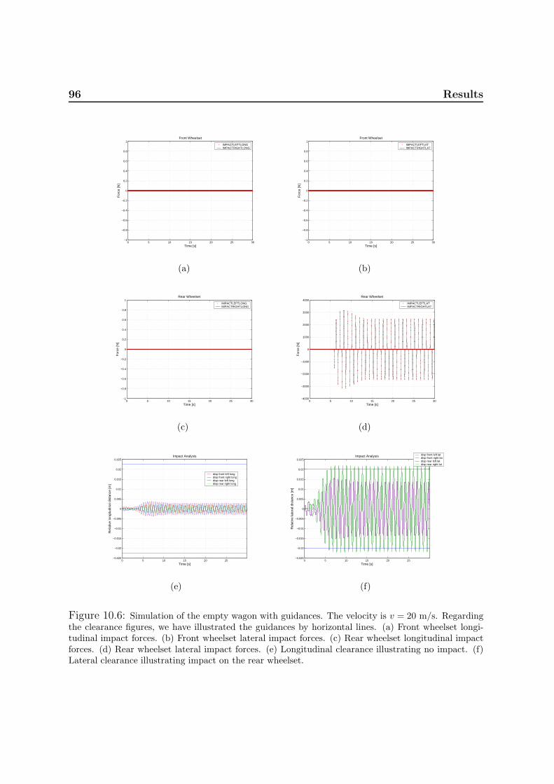
96 Results
0 5 10 15 20 25 30−1
−0.8
−0.6
−0.4
−0.2
0
0.2
0.4
0.6
0.8
1
Time [s]
For
ce [N
]
Front Wheelset
IMPACTLEFTLONGIMPACTRIGHTLONG
(a)
0 5 10 15 20 25 30−1
−0.8
−0.6
−0.4
−0.2
0
0.2
0.4
0.6
0.8
1
Time [s]
For
ce [N
]
Front Wheelset
IMPACTLEFTLATIMPACTRIGHTLAT
(b)
0 5 10 15 20 25 30−1
−0.8
−0.6
−0.4
−0.2
0
0.2
0.4
0.6
0.8
1
Time [s]
For
ce [N
]
Rear Wheelset
IMPACTLEFTLONGIMPACTRIGHTLONG
(c)
0 5 10 15 20 25 30−4000
−3000
−2000
−1000
0
1000
2000
3000
4000
Time [s]
For
ce [N
]Rear Wheelset
IMPACTLEFTLATIMPACTRIGHTLAT
(d)
0 5 10 15 20 25−0.025
−0.02
−0.015
−0.01
−0.005
0
0.005
0.01
0.015
0.02
0.025
Time [s]
Rel
ativ
e lo
ngitu
dina
l dis
tanc
e [m
]
Impact Analysis
disp front left longdisp front right longdisp rear left longdisp rear right long
(e)
0 5 10 15 20 25−0.025
−0.02
−0.015
−0.01
−0.005
0
0.005
0.01
0.015
0.02
0.025
Time [s]
Rel
ativ
e la
tera
l dis
tanc
e [m
]
Impact Analysis disp front left latdisp front right latdisp rear left latdisp rear right lat
(f)
Figure 10.6: Simulation of the empty wagon with guidances. The velocity is v = 20 m/s. Regardingthe clearance figures, we have illustrated the guidances by horizontal lines. (a) Front wheelset longi-tudinal impact forces. (b) Front wheelset lateral impact forces. (c) Rear wheelset longitudinal impactforces. (d) Rear wheelset lateral impact forces. (e) Longitudinal clearance illustrating no impact. (f)Lateral clearance illustrating impact on the rear wheelset.
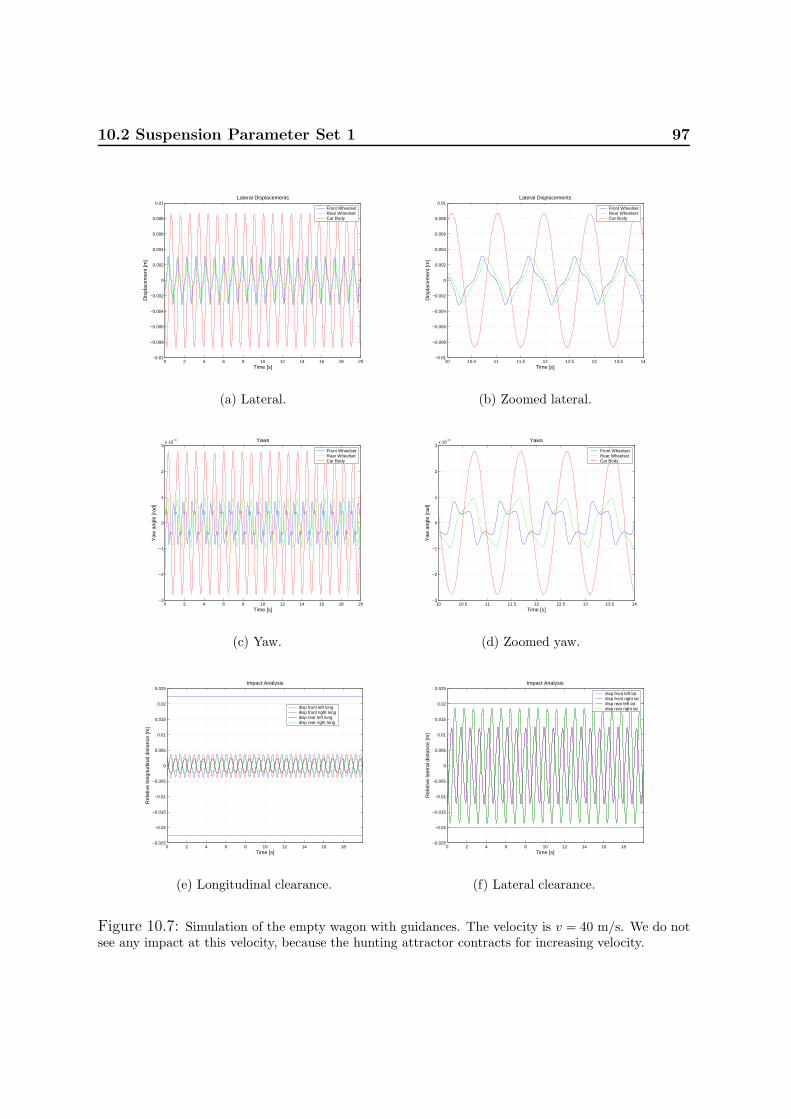
10.2 Suspension Parameter Set 1 97
0 2 4 6 8 10 12 14 16 18 20−0.01
−0.008
−0.006
−0.004
−0.002
0
0.002
0.004
0.006
0.008
0.01
Time [s]
Dis
plac
emen
t [m
]
Lateral Displacements
Front WheelsetRear WheelsetCar Body
(a) Lateral.
10 10.5 11 11.5 12 12.5 13 13.5 14−0.01
−0.008
−0.006
−0.004
−0.002
0
0.002
0.004
0.006
0.008
0.01
Time [s]
Dis
plac
emen
t [m
]
Lateral Displacements
Front WheelsetRear WheelsetCar Body
(b) Zoomed lateral.
0 2 4 6 8 10 12 14 16 18 20−3
−2
−1
0
1
2
3x 10
−3
Time [s]
Yaw
ang
le [r
ad]
Yaws
Front WheelsetRear WheelsetCar Body
(c) Yaw.
10 10.5 11 11.5 12 12.5 13 13.5 14−3
−2
−1
0
1
2
3x 10
−3
Time [s]
Yaw
ang
le [r
ad]
Yaws
Front WheelsetRear WheelsetCar Body
(d) Zoomed yaw.
0 2 4 6 8 10 12 14 16 18−0.025
−0.02
−0.015
−0.01
−0.005
0
0.005
0.01
0.015
0.02
0.025
Time [s]
Rel
ativ
e lo
ngitu
dina
l dis
tanc
e [m
]
Impact Analysis
disp front left longdisp front right longdisp rear left longdisp rear right long
(e) Longitudinal clearance.
0 2 4 6 8 10 12 14 16 18−0.025
−0.02
−0.015
−0.01
−0.005
0
0.005
0.01
0.015
0.02
0.025
Time [s]
Rel
ativ
e la
tera
l dis
tanc
e [m
]
Impact Analysis
disp front left latdisp front right latdisp rear left latdisp rear right lat
(f) Lateral clearance.
Figure 10.7: Simulation of the empty wagon with guidances. The velocity is v = 40 m/s. We do notsee any impact at this velocity, because the hunting attractor contracts for increasing velocity.

98 Results
Empty wagon running at v = 15 m/s
We can observe in the following figures that lateral movement of the wheelsets is rel-atively smooth, and that only the rear wheelset experiences impact with the freightwagon.
0 10 20 30 40 50 60−0.025
−0.02
−0.015
−0.01
−0.005
0
0.005
0.01
0.015
0.02
0.025
Time [s]
Dis
plac
emen
t [m
]
Lateral Displacements
Front WheelsetRear WheelsetCar Body
(a)
40 40.5 41 41.5 42 42.5 43 43.5 44 44.5 45−5
−4
−3
−2
−1
0
1
2
3
4
5x 10
−3
Time [s]
Dis
plac
emen
t [m
]
Lateral Displacements
Front WheelsetRear Wheelset
(b)
0 10 20 30 40 50 60−2.5
−2
−1.5
−1
−0.5
0
0.5
1
1.5
2
2.5x 10
−3
Time [s]
Yaw
ang
le [r
ad]
Yaws
Front WheelsetRear WheelsetCar Body
(c)
40 40.5 41 41.5 42 42.5 43 43.5 44 44.5 45−3
−2
−1
0
1
2
3x 10
−3
Time [s]
Yaw
ang
le [r
ad]
Yaws
Front WheelsetRear WheelsetCar Body
(d)
Figure 10.8: Simulation results of the empty wagon running at v = 15 m/s. (a) Lateral displacement.(b) Zoomed lateral displacement, excluding car body lateral displacement. (c) Yaw angle. (d) Zoomedyaw angle.

10.2 Suspension Parameter Set 1 99
0 10 20 30 40 50 60−1
−0.8
−0.6
−0.4
−0.2
0
0.2
0.4
0.6
0.8
1
Time [s]
For
ce [N
]
Front Wheelset
IMPACTLEFTLATIMPACTRIGHTLAT
(a)
0 10 20 30 40 50 60−3000
−2000
−1000
0
1000
2000
3000
Time [s]
For
ce [N
]
Rear Wheelset
IMPACTLEFTLATIMPACTRIGHTLAT
(b)
0 10 20 30 40 50 60−0.025
−0.02
−0.015
−0.01
−0.005
0
0.005
0.01
0.015
0.02
0.025
Time [s]
Rel
ativ
e lo
ngitu
dina
l dis
tanc
e [m
]
Impact Analysis
disp front left longdisp front right longdisp rear left longdisp rear right long
(c)
40 40.5 41 41.5 42 42.5 43 43.5 44 44.5 45−0.03
−0.02
−0.01
0
0.01
0.02
0.03
Time [s]
Rel
ativ
e lo
ngitu
dina
l dis
tanc
e [m
]Impact Analysis
disp front left longdisp front right longdisp rear left longdisp rear right long
(d)
0 10 20 30 40 50 60−0.025
−0.02
−0.015
−0.01
−0.005
0
0.005
0.01
0.015
0.02
0.025
Time [s]
Rel
ativ
e la
tera
l dis
tanc
e [m
]
Impact Analysis
disp front left latdisp front right latdisp rear left latdisp rear right lat
(e)
40 40.5 41 41.5 42 42.5 43 43.5 44 44.5 45−0.03
−0.02
−0.01
0
0.01
0.02
0.03
Time [s]
Rel
ativ
e la
tera
l dis
tanc
e [m
]
Impact Analysis
disp front left latdisp front right latdisp rear left latdisp rear right lat
(f)
Figure 10.9: Impact analysis of the empty wagon running at v = 15 m/s. (a) Front wheelset lateralimpact forces. (b) Rear wheelset lateral impact forces. (c) Longitudinal clearances. (d) Zoomedlongitudinal clearance. (e) Lateral clearances. (f) Zoomed lateral clearances.

100 Results
Empty wagon running at v = 13 m/s
We observe in the following figures that lateral movement of the front wheelsets is nolonger smooth, especially the movement of the rear wheelset.
In observing the lateral clearances, we see that both wheelsets now impact, and theforces are comparable to each other, although the rear wheelset impacts with greaterforce. Thus the discontinuity at about 14 m/s is probably brought about a transitionfrom only the rear wheelset impacting, to both wheelsets impacting.
0 10 20 30 40 50 60−0.03
−0.02
−0.01
0
0.01
0.02
0.03
Time [s]
Dis
plac
emen
t [m
]
Lateral Displacements
Front WheelsetRear WheelsetCar Body
(a)
40 40.5 41 41.5 42 42.5 43 43.5 44 44.5 45−0.01
−0.008
−0.006
−0.004
−0.002
0
0.002
0.004
0.006
0.008
0.01
Time [s]
Dis
plac
emen
t [m
]
Lateral Displacements
Front WheelsetRear Wheelset
(b)
0 10 20 30 40 50 60−8
−6
−4
−2
0
2
4
6
8x 10
−3
Time [s]
Yaw
ang
le [r
ad]
Yaws
Front WheelsetRear WheelsetCar Body
(c)
40 40.5 41 41.5 42 42.5 43 43.5 44 44.5 45−0.01
−0.008
−0.006
−0.004
−0.002
0
0.002
0.004
0.006
0.008
0.01
Time [s]
Yaw
ang
le [r
ad]
Yaws
Front WheelsetRear WheelsetCar Body
(d)
Figure 10.10: Simulation results of the empty wagon running at v = 13 m/s. (a) Lateral displacement.(b) Zoomed lateral displacement, excluding car body lateral displacement. (c) Yaw angle. (d) Zoomedyaw angle.
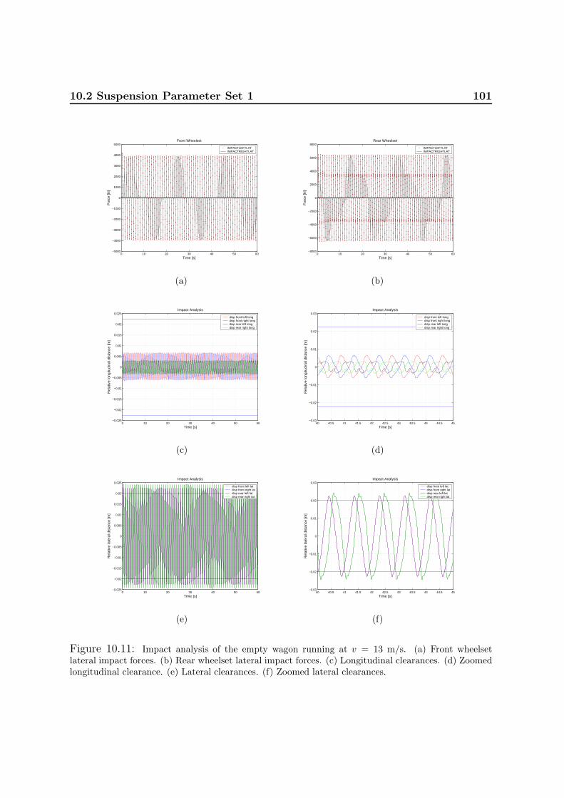
10.2 Suspension Parameter Set 1 101
0 10 20 30 40 50 60−5000
−4000
−3000
−2000
−1000
0
1000
2000
3000
4000
5000
Time [s]
For
ce [N
]
Front Wheelset
IMPACTLEFTLATIMPACTRIGHTLAT
(a)
0 10 20 30 40 50 60−8000
−6000
−4000
−2000
0
2000
4000
6000
8000
Time [s]
For
ce [N
]
Rear Wheelset
IMPACTLEFTLATIMPACTRIGHTLAT
(b)
0 10 20 30 40 50 60−0.025
−0.02
−0.015
−0.01
−0.005
0
0.005
0.01
0.015
0.02
0.025
Time [s]
Rel
ativ
e lo
ngitu
dina
l dis
tanc
e [m
]
Impact Analysis
disp front left longdisp front right longdisp rear left longdisp rear right long
(c)
40 40.5 41 41.5 42 42.5 43 43.5 44 44.5 45−0.03
−0.02
−0.01
0
0.01
0.02
0.03
Time [s]
Rel
ativ
e lo
ngitu
dina
l dis
tanc
e [m
]Impact Analysis
disp front left longdisp front right longdisp rear left longdisp rear right long
(d)
0 10 20 30 40 50 60−0.025
−0.02
−0.015
−0.01
−0.005
0
0.005
0.01
0.015
0.02
0.025
Time [s]
Rel
ativ
e la
tera
l dis
tanc
e [m
]
Impact Analysis
disp front left latdisp front right latdisp rear left latdisp rear right lat
(e)
40 40.5 41 41.5 42 42.5 43 43.5 44 44.5 45−0.03
−0.02
−0.01
0
0.01
0.02
0.03
Time [s]
Rel
ativ
e la
tera
l dis
tanc
e [m
]
Impact Analysis
disp front left latdisp front right latdisp rear left latdisp rear right lat
(f)
Figure 10.11: Impact analysis of the empty wagon running at v = 13 m/s. (a) Front wheelsetlateral impact forces. (b) Rear wheelset lateral impact forces. (c) Longitudinal clearances. (d) Zoomedlongitudinal clearance. (e) Lateral clearances. (f) Zoomed lateral clearances.

102 Results
Empty wagon running at v = 11 m/s
In order to investigate the discontinuity at about 10 m/s in the lateral behaviour of thefreight wagon body, we performed simulations for 11 m/s and 9.5 m/s. Here, at 11 m/s,we can ascertain that behaviour is relatively similar to that for 13 m/s. Cheifly, bothwheelsets are impacting against the freight wagon body, and with more or less the sameintensity. In particular, the movement of the rear wheelset laterally is still erratic at itsextrema.
0 10 20 30 40 50 60−0.03
−0.02
−0.01
0
0.01
0.02
0.03
Time [s]
Dis
plac
emen
t [m
]
Lateral Displacements
Front WheelsetRear WheelsetCar Body
(a)
40 40.5 41 41.5 42 42.5 43 43.5 44 44.5 45−0.01
−0.008
−0.006
−0.004
−0.002
0
0.002
0.004
0.006
0.008
0.01
Time [s]
Dis
plac
emen
t [m
]
Lateral Displacements
Front WheelsetRear Wheelset
(b)
0 10 20 30 40 50 60−8
−6
−4
−2
0
2
4
6
8x 10
−3
Time [s]
Yaw
ang
le [r
ad]
Yaws
Front WheelsetRear WheelsetCar Body
(c)
40 40.5 41 41.5 42 42.5 43 43.5 44 44.5 45−0.01
−0.008
−0.006
−0.004
−0.002
0
0.002
0.004
0.006
0.008
0.01
Time [s]
Yaw
ang
le [r
ad]
Yaws
Front WheelsetRear WheelsetCar Body
(d)
Figure 10.12: Simulation results of the empty wagon running at v = 11 m/s. (a) Lateral displacement.(b) Zoomed lateral displacement, excluding car body lateral displacement. (c) Yaw angle. (d) Zoomedyaw angle.

10.2 Suspension Parameter Set 1 103
0 10 20 30 40 50 60−4000
−3000
−2000
−1000
0
1000
2000
3000
4000
Time [s]
For
ce [N
]
Front Wheelset
IMPACTLEFTLATIMPACTRIGHTLAT
(a)
0 10 20 30 40 50 60−8000
−6000
−4000
−2000
0
2000
4000
6000
8000
Time [s]
For
ce [N
]
Rear Wheelset
IMPACTLEFTLATIMPACTRIGHTLAT
(b)
0 10 20 30 40 50 60−0.025
−0.02
−0.015
−0.01
−0.005
0
0.005
0.01
0.015
0.02
0.025
Time [s]
Rel
ativ
e lo
ngitu
dina
l dis
tanc
e [m
]
Impact Analysis
disp front left longdisp front right longdisp rear left longdisp rear right long
(c)
40 40.5 41 41.5 42 42.5 43 43.5 44 44.5 45−0.03
−0.02
−0.01
0
0.01
0.02
0.03
Time [s]
Rel
ativ
e lo
ngitu
dina
l dis
tanc
e [m
]Impact Analysis
disp front left longdisp front right longdisp rear left longdisp rear right long
(d)
0 10 20 30 40 50 60−0.025
−0.02
−0.015
−0.01
−0.005
0
0.005
0.01
0.015
0.02
0.025
Time [s]
Rel
ativ
e la
tera
l dis
tanc
e [m
]
Impact Analysis
disp front left latdisp front right latdisp rear left latdisp rear right lat
(e)
40 40.5 41 41.5 42 42.5 43 43.5 44 44.5 45−0.03
−0.02
−0.01
0
0.01
0.02
0.03
Time [s]
Rel
ativ
e la
tera
l dis
tanc
e [m
]
Impact Analysis
disp front left latdisp front right latdisp rear left latdisp rear right lat
(f)
Figure 10.13: Impact analysis of the empty wagon running at v = 11 m/s. (a) Front wheelsetlateral impact forces. (b) Rear wheelset lateral impact forces. (c) Longitudinal clearances. (d) Zoomedlongitudinal clearance. (e) Lateral clearances. (f) Zoomed lateral clearances.

104 Results
Empty wagon running at v = 9.5 m/s
At v = 9.5 m/s we can observe that behaviour is different that for v = 11 m/s. Ofinterest is the fact that although both wheelset still impact laterally against the freightwagon body, the rear wheelset no longer behaves erratically at its extrema.
In that both wheelsets still impact laterally, no significant effect is seen on the bi-furcation trace of any discontinuity with respect to either wheelset hunting, but thediscrepancy is located with the lateral hunting of the car body. This jump can comeabout due to a change in the way forces are imparted upon the car body from thewheelsets during impact, in that now they are smoother than the erratic rear wheelsetimpacts experienced at v = 11 m/s.
0 10 20 30 40 50 60−0.03
−0.02
−0.01
0
0.01
0.02
0.03
Time [s]
Dis
plac
emen
t [m
]
Lateral Displacements
Front WheelsetRear WheelsetCar Body
(a)
40 40.5 41 41.5 42 42.5 43 43.5 44 44.5 45−0.01
−0.008
−0.006
−0.004
−0.002
0
0.002
0.004
0.006
0.008
0.01
Time [s]
Dis
plac
emen
t [m
]
Lateral Displacements
Front WheelsetRear Wheelset
(b)
0 10 20 30 40 50 60−5
−4
−3
−2
−1
0
1
2
3
4
5x 10
−3
Time [s]
Yaw
ang
le [r
ad]
Yaws
Front WheelsetRear WheelsetCar Body
(c)
40 40.5 41 41.5 42 42.5 43 43.5 44 44.5 45−5
−4
−3
−2
−1
0
1
2
3
4
5x 10
−3
Time [s]
Yaw
ang
le [r
ad]
Yaws
Front WheelsetRear WheelsetCar Body
(d)
Figure 10.14: Simulation results of the empty wagon running at v = 9.5 m/s. (a) Lateral displace-ment. (b) Zoomed lateral displacement, excluding car body lateral displacement. (c) Yaw angle. (d)Zoomed yaw angle.

10.2 Suspension Parameter Set 1 105
0 10 20 30 40 50 60−1500
−1000
−500
0
500
1000
1500
2000
Time [s]
For
ce [N
]
Front Wheelset
IMPACTLEFTLATIMPACTRIGHTLAT
(a)
0 10 20 30 40 50 60−3000
−2000
−1000
0
1000
2000
3000
Time [s]
For
ce [N
]
Rear Wheelset
IMPACTLEFTLATIMPACTRIGHTLAT
(b)
0 10 20 30 40 50 60−0.025
−0.02
−0.015
−0.01
−0.005
0
0.005
0.01
0.015
0.02
0.025
Time [s]
Rel
ativ
e lo
ngitu
dina
l dis
tanc
e [m
]
Impact Analysis
disp front left longdisp front right longdisp rear left longdisp rear right long
(c)
40 40.5 41 41.5 42 42.5 43 43.5 44 44.5 45−0.03
−0.02
−0.01
0
0.01
0.02
0.03
Time [s]
Rel
ativ
e lo
ngitu
dina
l dis
tanc
e [m
]Impact Analysis
disp front left longdisp front right longdisp rear left longdisp rear right long
(d)
0 10 20 30 40 50 60−0.025
−0.02
−0.015
−0.01
−0.005
0
0.005
0.01
0.015
0.02
0.025
Time [s]
Rel
ativ
e la
tera
l dis
tanc
e [m
]
Impact Analysis
disp front left latdisp front right latdisp rear left latdisp rear right lat
(e)
40 40.5 41 41.5 42 42.5 43 43.5 44 44.5 45−0.03
−0.02
−0.01
0
0.01
0.02
0.03
Time [s]
Rel
ativ
e la
tera
l dis
tanc
e [m
]
Impact Analysis
disp front left latdisp front right latdisp rear left latdisp rear right lat
(f)
Figure 10.15: Impact analysis of the empty wagon running at v = 9.5 m/s. (a) Front wheelsetlateral impact forces. (b) Rear wheelset lateral impact forces. (c) Longitudinal clearances. (d) Zoomedlongitudinal clearance. (e) Lateral clearances. (f) Zoomed lateral clearances.

106 Results
Water loaded wagon running at v = 20 m/s
We here present time series data for a water loaded freight wagon running at v = 20 m/s.After an initial transient, we see that the wagon settles into a low frequency huntingoscillation.
What merits special attention here is the impact behaviour of the wheelsets. The rearwheelset dominates in this role, since it is clearly the one impacting hardest. The frontwheelset impacts, but not as hard as the rear wheelset. In fact, as velocity increases,the front wheelset will not impact at all with the freight wagon structure. Eventually,the rear wheelset won’t either, given sufficient velocity.
0 5 10 15 20 25 30−0.03
−0.02
−0.01
0
0.01
0.02
0.03
Time [s]
Dis
plac
emen
t [m
]
Lateral Displacements
Front WheelsetRear WheelsetCar Body
(a)
12 13 14 15 16 17 18 19 20 21 22−5
−4
−3
−2
−1
0
1
2
3
4
5x 10
−3
Time [s]
Dis
plac
emen
t [m
]
Lateral Displacements
Front WheelsetRear Wheelset
(b)
0 5 10 15 20 25 30−3
−2
−1
0
1
2
3x 10
−3
Time [s]
Yaw
ang
le [r
ad]
Yaws
Front WheelsetRear WheelsetCar Body
(c)
12 13 14 15 16 17 18 19 20 21 22−3
−2
−1
0
1
2
3x 10
−3
Time [s]
Yaw
ang
le [r
ad]
Yaws
Front WheelsetRear WheelsetCar Body
(d)
Figure 10.16: Simulation results of the water loaded wagon running at v = 20 m/s. (a) Lateraldisplacement. (b) Zoomed lateral displacement, excluding car body lateral displacement. (c) Yawangle. (d) Zoomed yaw angle.
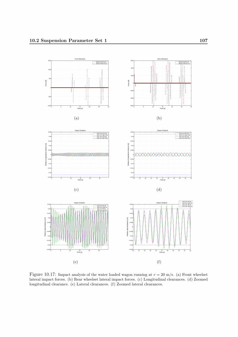
10.2 Suspension Parameter Set 1 107
0 5 10 15 20 25 30−1000
−500
0
500
1000
1500
Time [s]
For
ce [N
]
Front Wheelset
IMPACTLEFTLATIMPACTRIGHTLAT
(a)
0 5 10 15 20 25 30−6000
−4000
−2000
0
2000
4000
6000
Time [s]
For
ce [N
]
Rear Wheelset
IMPACTLEFTLATIMPACTRIGHTLAT
(b)
0 5 10 15 20 25−0.025
−0.02
−0.015
−0.01
−0.005
0
0.005
0.01
0.015
0.02
0.025
Time [s]
Rel
ativ
e lo
ngitu
dina
l dis
tanc
e [m
]
Impact Analysis
disp front left longdisp front right longdisp rear left longdisp rear right long
(c)
12 13 14 15 16 17 18 19 20 21 22−0.025
−0.02
−0.015
−0.01
−0.005
0
0.005
0.01
0.015
0.02
0.025
Time [s]
Rel
ativ
e lo
ngitu
dina
l dis
tanc
e [m
]
Impact Analysis
disp front left longdisp front right longdisp rear left longdisp rear right long
(d)
0 5 10 15 20 25−0.025
−0.02
−0.015
−0.01
−0.005
0
0.005
0.01
0.015
0.02
0.025
Time [s]
Rel
ativ
e la
tera
l dis
tanc
e [m
]
Impact Analysis
disp front left latdisp front right latdisp rear left latdisp rear right lat
(e)
12 13 14 15 16 17 18 19 20 21 22−0.025
−0.02
−0.015
−0.01
−0.005
0
0.005
0.01
0.015
0.02
0.025
Time [s]
Rel
ativ
e la
tera
l dis
tanc
e [m
]
Impact Analysisdisp front left latdisp front right latdisp rear left latdisp rear right lat
(f)
Figure 10.17: Impact analysis of the water loaded wagon running at v = 20 m/s. (a) Front wheelsetlateral impact forces. (b) Rear wheelset lateral impact forces. (c) Longitudinal clearances. (d) Zoomedlongitudinal clearance. (e) Lateral clearances. (f) Zoomed lateral clearances.

108 Results
Water loaded wagon running at v = 18 m/s
After an initial transient, we see that the wagon settles into a low frequency huntingoscillation. Here, we take special note of the impact behaviour of the wheelsets. Bothwheelsets now impact forcefully with the freight wagon structure, with nearly equalvigour. This indicates to us that the transition that takes place near the v = 19 m/smark on the bifurcation trace figure 10.1(c) is one where the front wheelset begins toirritate the dynamics of the freight wagon more and more as it begins to impact, and itsimpacts increase in strength. Furthermore, the long period behaviour is what seems tolend a chaotic pattern to the bifurcation trace figure 10.1(c), but since we only samplethe values for the bifurcation traces over a 3 second interval, we evade considering anentire wavelength of data, and thus we produce what seems to be a chaotic transitionin the bifurcation trace.
0 5 10 15 20 25 30−0.05
−0.04
−0.03
−0.02
−0.01
0
0.01
0.02
0.03
0.04
0.05
Time [s]
Dis
plac
emen
t [m
]
Lateral Displacements
Front WheelsetRear WheelsetCar Body
(a)
20 21 22 23 24 25 26−0.01
−0.008
−0.006
−0.004
−0.002
0
0.002
0.004
0.006
0.008
0.01
Time [s]
Dis
plac
emen
t [m
]
Lateral Displacements
Front WheelsetRear Wheelset
(b)
0 5 10 15 20 25 30−10
−8
−6
−4
−2
0
2
4
6
8x 10
−3
Time [s]
Yaw
ang
le [r
ad]
Yaws
Front WheelsetRear WheelsetCar Body
(c)
20 21 22 23 24 25 26−8
−6
−4
−2
0
2
4
6
8x 10
−3
Time [s]
Yaw
ang
le [r
ad]
Yaws
Front WheelsetRear WheelsetCar Body
(d)
Figure 10.18: Simulation results of the water loaded wagon running at v = 18 m/s. (a) Lateraldisplacement. (b) Zoomed lateral displacement, excluding car body lateral displacement. (c) Yawangle. (d) Zoomed yaw angle.

10.2 Suspension Parameter Set 1 109
0 5 10 15 20 25 30−1.5
−1
−0.5
0
0.5
1
1.5x 10
4
Time [s]
For
ce [N
]
Front Wheelset
IMPACTLEFTLATIMPACTRIGHTLAT
(a)
0 5 10 15 20 25 30−2
−1.5
−1
−0.5
0
0.5
1
1.5
2x 10
4
Time [s]
For
ce [N
]
Rear Wheelset
IMPACTLEFTLATIMPACTRIGHTLAT
(b)
0 5 10 15 20 25 30−0.025
−0.02
−0.015
−0.01
−0.005
0
0.005
0.01
0.015
0.02
0.025
Time [s]
Rel
ativ
e lo
ngitu
dina
l dis
tanc
e [m
]
Impact Analysis
disp front left longdisp front right longdisp rear left longdisp rear right long
(c)
20 21 22 23 24 25 26−0.025
−0.02
−0.015
−0.01
−0.005
0
0.005
0.01
0.015
0.02
0.025
Time [s]
Rel
ativ
e lo
ngitu
dina
l dis
tanc
e [m
]Impact Analysis
disp front left longdisp front right longdisp rear left longdisp rear right long
(d)
0 5 10 15 20 25 30−0.04
−0.03
−0.02
−0.01
0
0.01
0.02
0.03
0.04
Time [s]
Rel
ativ
e la
tera
l dis
tanc
e [m
]
Impact Analysis
disp front left latdisp front right latdisp rear left latdisp rear right lat
(e)
20 21 22 23 24 25 26−0.04
−0.03
−0.02
−0.01
0
0.01
0.02
0.03
0.04
Time [s]
Rel
ativ
e la
tera
l dis
tanc
e [m
]
Impact Analysisdisp front left latdisp front right latdisp rear left latdisp rear right lat
(f)
Figure 10.19: Impact analysis of the water loaded wagon running at v = 18 m/s. (a) Front wheelsetlateral impact forces. (b) Rear wheelset lateral impact forces. (c) Longitudinal clearances. (d) Zoomedlongitudinal clearance. (e) Lateral clearances. (f) Zoomed lateral clearances.

110 Results
Packed wagon running at v = 17 m/s
The strange behaviour in the bifurcation trace in the case of the packed wagon occursas we slow down towards the nonlinear critical velocity. What actually occurs is that anew frequency is introduced in the lateral hunting motion. The period of this is beyondthe 3 second sampling time, and introduces this strange behaviour in the bifurcationdiagram. Had the sampling time been longer, we could have avoided this behaviour, butmay have missed the fact that the hunting period begins to change.
In this section, we present a series of figures which illustrate the behaviour of thepacked freight wagon at v = 17 m/s, which resides in this ‘strange’ region on thebifurcation trace. We clearly see that the period is about 8 seconds, which is clearlylarger than the 3 second sampling time we use.
0 5 10 15 20 25 30−0.025
−0.02
−0.015
−0.01
−0.005
0
0.005
0.01
0.015
0.02
0.025
Time [s]
Dis
plac
emen
t [m
]
Lateral Displacements
Front WheelsetRear WheelsetCar Body
(a)
18 18.5 19 19.5 20 20.5 21 21.5 22 22.5 23−0.025
−0.02
−0.015
−0.01
−0.005
0
0.005
0.01
0.015
0.02
0.025
Time [s]
Dis
plac
emen
t [m
]Lateral Displacements
Front WheelsetRear WheelsetCar Body
(b)
0 5 10 15 20 25 30−2.5
−2
−1.5
−1
−0.5
0
0.5
1
1.5
2
2.5x 10
−3
Time [s]
Yaw
ang
le [r
ad]
Yaws
Front WheelsetRear WheelsetCar Body
(c)
18 18.5 19 19.5 20 20.5 21 21.5 22 22.5 23−2.5
−2
−1.5
−1
−0.5
0
0.5
1
1.5
2
2.5x 10
−3
Time [s]
Yaw
ang
le [r
ad]
Yaws
Front WheelsetRear WheelsetCar Body
(d)
Figure 10.20: Simulation results of the packed wagon running at v = 17 m/s. (a) Lateral displace-ment. (b) Zoomed lateral displacement, excluding car body lateral displacement. (c) Yaw angle. (d)Zoomed yaw angle.

10.2 Suspension Parameter Set 1 111
0 5 10 15 20 25 30−1
−0.8
−0.6
−0.4
−0.2
0
0.2
0.4
0.6
0.8
1
Time [s]
For
ce [N
]
Front Wheelset
IMPACTLEFTLATIMPACTRIGHTLAT
(a)
0 5 10 15 20 25 30−5000
−4000
−3000
−2000
−1000
0
1000
2000
3000
4000
5000
Time [s]
For
ce [N
]
Rear Wheelset
IMPACTLEFTLATIMPACTRIGHTLAT
(b)
0 5 10 15 20 25−0.025
−0.02
−0.015
−0.01
−0.005
0
0.005
0.01
0.015
0.02
0.025
Time [s]
Rel
ativ
e lo
ngitu
dina
l dis
tanc
e [m
]
Impact Analysis
disp front left longdisp front right longdisp rear left longdisp rear right long
(c)
18 18.5 19 19.5 20 20.5 21 21.5 22 22.5 23−0.025
−0.02
−0.015
−0.01
−0.005
0
0.005
0.01
0.015
0.02
0.025
Time [s]
Rel
ativ
e lo
ngitu
dina
l dis
tanc
e [m
]
Impact Analysis
disp front left longdisp front right longdisp rear left longdisp rear right long
(d)
0 5 10 15 20 25−0.025
−0.02
−0.015
−0.01
−0.005
0
0.005
0.01
0.015
0.02
0.025
Time [s]
Rel
ativ
e la
tera
l dis
tanc
e [m
]
Impact Analysis
disp front left latdisp front right latdisp rear left latdisp rear right lat
(e)
18 18.5 19 19.5 20 20.5 21 21.5 22 22.5 23−0.025
−0.02
−0.015
−0.01
−0.005
0
0.005
0.01
0.015
0.02
0.025
Time [s]
Rel
ativ
e la
tera
l dis
tanc
e [m
]
Impact Analysis
disp front left latdisp front right latdisp rear left latdisp rear right lat
(f)
Figure 10.21: Impact analysis of the packed wagon running at v = 17 m/s. (a) Front wheelsetlateral impact forces. (b) Rear wheelset lateral impact forces. (c) Longitudinal clearances. (d) Zoomedlongitudinal clearance. (e) Lateral clearances. (f) Zoomed lateral clearances.

112 Results
10.3 Suspension Parameter Set 2
10.3.1 Critical Velocities
We have here calculated bifurcation traces for a freight wagon using suspension param-eter set 2. These are presented in figures 10.22 and 10.23. Similar to the bifurcationtraces for suspension parameter set 1 we see that the amplitude of the hunting motionincreases as the velocity is lowered towards the nonlinear critical velcoity in the emptyand water loaded case. For the packed wagon, the situation is quite different in that thelarge hysteresis loop seems to be gone.
In contrast to the bifurcation diagrams for the first suspension parameter set wedo not see any discontinuities in the bifurcation diagram. The general picture now isa better dynamic behaviour for the freight wagon. Especially, the amplitude of thehunting motion for the car body is reduced.
This tendency is, however, not surprising. We described in the chapter 4 that thecharacteristic difference between the two suspension parameter sets is that suspensionparameter set 2 dissipates more energy. Thus when comparing two freight wagons withdifferent dissipation abilities in the suspension it might be reasonable to expect that thewagon with best dissipation capability has the best running properties.
Furthermore, figure 10.22(b) details the bifurcation trace for the front wheelset inthe empty freight wagon case. An interesting view is to zoom in on this figure (see10.22(c)), because it illustrates the effect of dry friction present in the suspension. Theeffect is that the stable equilibrium in the center of the track is shifted slightly after onerevolution in the hysteresis loop. This behaviour is similar to the one predicted by thesimple dry friction system earlier investigated, and we see it’s effect here.
As we proceed to analyse the packed wagon, the qualitative behaviour changed com-pletely as shown in the bifurcation trace in figure 10.23(b). The saddle node bifurcationthat defines the nonlinear critical velocity seems to be gone, although it still looks likethere is some hysteresis present. However, the prediction of the hysteresis loop is notcorrect, because it is created by the delay phenomenon in our bifurcation trace method.This conclusion was revealed in the following manner.
By making an eigenvalue analysis of the centered position we found that there is aHopf bifurcation taking place at v = 33.7 m/s. Figure 10.24 shows how the eigenvaluescrosses the imaginary axis just around the critical velocity. At this point we do not knowwhether the Hopf bifurcation is supercritical or subcritical. By examining the asymptoticsolution for velocities slightly greater than the critical velocity we found an increasinglimit cycle corresponding to the one shown in the bifurcation diagram. An exampleof this is shown in figure 10.25. This figure illustrates two important properties of thesystem. First, it is shown how long time it takes to reach the asymptotic solution (whichin fact is the origin of the delay problem in the bifurcation trace method). Secondly, bycomparing amplitudes (see zoomed view in figure 10.25(b)) we see that the asymptotic

10.3 Suspension Parameter Set 2 113
solution is the one predicted in the bifurcation diagram in figure 10.23(b). The conclusionfrom this is that the Hopf bifurcation is supercritical.
Although not found, we emphasize the existence of a distant, undiscovered huntingattractor is possible in the case of the packed wagon.
10 15 20 25 30 350
0.5
1
1.5
2
2.5
3
3.5
4
4.5x 10
−3
Velocity [m/s]
Max
. lat
eral
dis
plac
emen
t [m
]
Bifurcation Diagram for Parameter Set 2
Front wheelsetRear wheelsetCar body
(a)
10 15 20 25 30 350
0.5
1
1.5
2
2.5
3x 10
−3
Velocity [m/s]
Max
. lat
eral
dis
plac
emen
t [m
]
Bifurcation Diagram for Parameter Set 2 (FW)
Increasing vDecreasing v
(b)
12 14 16 18 20 22 24 26 28 300
1
2
3
4
5
x 10−5
Velocity [m/s]
Max
. lat
eral
dis
plac
emen
t [m
]
Bifurcation Diagram for Parameter Set 2 (FW)
Increasing vDecreasing v
(c)
Figure 10.22: (a) Bifurcation diagram for the empty freight wagon. (b) Bifurcation diagram forthe front wheelset emphasizing the different behaviour between increasing and decreasing the velocity.Especially, it is seen that the stable equilibrium in the center of track has changed after one lap in thehysteresis loop.

114 Results
15 20 25 30 35 400
0.5
1
1.5
2
2.5
3
3.5
4
4.5
5x 10
−3
Velocity [m/s]
Max
. lat
eral
dis
plac
emen
t [m
]
Bifurcation Diagram for Parameter Set 2
Front wheelsetRear wheelsetCar body
(a)
15 20 25 30 35 400
0.5
1
1.5x 10
−3
Velocity [m/s]
Max
. lat
eral
dis
plac
emen
t [m
]
Bifurcation Diagram for Parameter Set 2
Front wheelsetRear wheelsetCar body
(b)
Figure 10.23: (a) Bifurcation diagram for the water loaded wagon. (b) Bifurcation diagram for thepacked freight wagon. Regarding the packed freight wagon we observe a small hysteresis loop, however,further analysis revealed that we have a supercritical Hopf bifurcation exhibiting no hysteresis. Thehysteresis loop oberserved is a consequence of the delay phenomenon present in our bifurcation tracemethod.
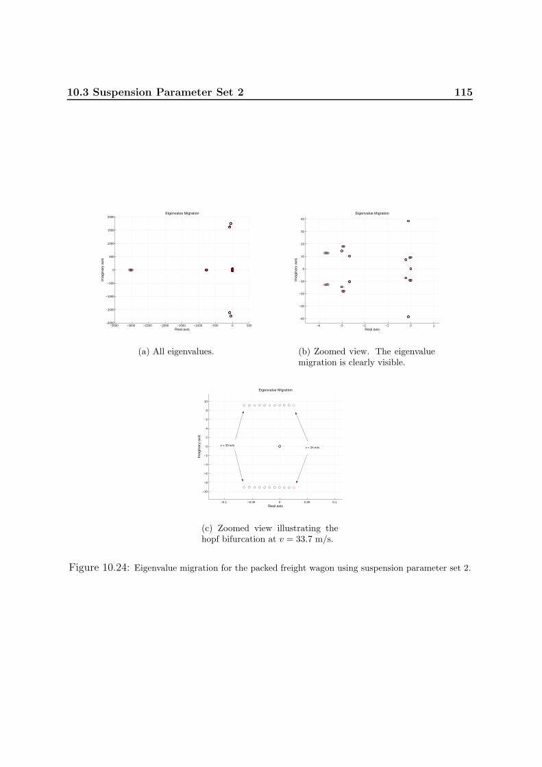
10.3 Suspension Parameter Set 2 115
−3500 −3000 −2500 −2000 −1500 −1000 −500 0 500−2000
−1500
−1000
−500
0
500
1000
1500
2000
Real axis
Imag
inar
y ax
is
Eigenvalue Migration
(a) All eigenvalues.
−4 −3 −2 −1 0 1
−40
−30
−20
−10
0
10
20
30
40
Real axis
Imag
inar
y ax
is
Eigenvalue Migration
(b) Zoomed view. The eigenvaluemigration is clearly visible.
−0.1 −0.05 0 0.05 0.1
−10
−8
−6
−4
−2
0
2
4
6
8
10
Real axis
Imag
inar
y ax
is
Eigenvalue Migration
v = 33 m/s v = 34 m/s
(c) Zoomed view illustrating thehopf bifurcation at v = 33.7 m/s.
Figure 10.24: Eigenvalue migration for the packed freight wagon using suspension parameter set 2.

116 Results
0 100 200 300 400 500 600−6
−4
−2
0
2
4
6x 10
−4
Time [s]
Dis
plac
emen
t [m
]
Lateral Displacements
Front WheelsetRear WheelsetCar Body
(a)
590 591 592 593 594 595 596 5974
5
6
x 10−4
Time [s]
Dis
plac
emen
t [m
]
Lateral Displacements
Front WheelsetRear WheelsetCar Body
(b)
Figure 10.25: (a) Time history at v = 34 m/s which is just above the Hopf bifurcation. The centerof the track is the initial condition and the figure illustrates how long time it takes to reach the huntingattractor. In this case it is approximately 530 s of simulation time. (b) Zoomed view of the timehistory. By comparing amplitudes it becomes evident that the attractor reached is the one shown inthe bifurcation diagram in figure 10.23(b).

10.3 Suspension Parameter Set 2 117
10.3.2 Guidance Impact Behaviour
Figure 10.26 illustrates the movement for the empty freight wagon at a velocity of 21m/s, close to the maximum lateral amplitude hunting movement in this case. In thisfigure, we can observe that the wheelset keeps itself well within the clearances afforded toit, and no impact occurs. This was in fact the result for all simulations with suspensionparameter set 2.
The fact that we did not observe any impact for suspension parameter set 2 dividesthe to suspension parameter set dramatically regarding the dynamic behaviour of thefreight wagon. Our explaination for this difference, in modelling the suspension linkswith the two parameter sets, is the fundamental difference in the dry friction dampingcapability between the two parameter sets.

118 Results
0 5 10 15 20 25 30−8
−6
−4
−2
0
2
4
6
8x 10
−5
Time [s]
Dis
plac
emen
t [m
]
Longitudinal Displacements
Front WheelsetRear Wheelset
(a) Longitudinal.
24 24.5 25 25.5 26 26.5 27 27.5 28 28.5 29−8
−6
−4
−2
0
2
4
6
8x 10
−5
Time [s]
Dis
plac
emen
t [m
]
Longitudinal Displacements
Front WheelsetRear Wheelset
(b) Zoomed longitudinal.
0 5 10 15 20 25 30−4
−3
−2
−1
0
1
2
3
4x 10
−3
Time [s]
Dis
plac
emen
t [m
]
Lateral DisplacementsFront WheelsetRear WheelsetCar Body
(c) Lateral.
24 24.5 25 25.5 26 26.5 27 27.5 28 28.5 29−4
−3
−2
−1
0
1
2
3
4x 10
−3
Time [s]
Dis
plac
emen
t [m
]
Lateral Displacements
Front WheelsetRear WheelsetCar Body
(d) Zoomed lateral.
0 5 10 15 20 25−0.025
−0.02
−0.015
−0.01
−0.005
0
0.005
0.01
0.015
0.02
0.025
Time [s]
Rel
ativ
e lo
ngitu
dina
l dis
tanc
e [m
]
Impact Analysis
disp front left longdisp front right longdisp rear left longdisp rear right long
(e) Longitudinal clearance.
0 5 10 15 20 25−0.025
−0.02
−0.015
−0.01
−0.005
0
0.005
0.01
0.015
0.02
0.025
Time [s]
Rel
ativ
e la
tera
l dis
tanc
e [m
]
Impact Analysis
disp front left latdisp front right latdisp rear left latdisp rear right lat
(f) Lateral clearance.
Figure 10.26: Impact investigation for the empty freight wagon using suspension parameter set 2.The velocity is v = 21 m/s.

10.4 Frequency Analysis 119
10.4 Frequency Analysis
In this section we will investigate which frequencies that are characteristic in the huntingmotion of our model. The result of the analysis is shown in table 10.1 and table 10.2.We have found the frequencies through a power spectrum analysis of each of the motionvariables given in the tables. The tables are supported by figures 10.27 to 10.30 thatillustrates this frequency analysis for some of the motion variables.
By looking at the results shown in the tables it becomes evident that given a certainconfiguration2 of the model leads to phase locked oscillations in the lateral and yawmotion of both wheelsets and car body as well as the roll motion of the car body. Thischaracteristic phase locked frequency at about 1 Hz is, however, not present in thelongitudinal displacement of wheelset. Regarding the longitudinal motion we see severalcharacteristic frequencies between 2 Hz and 6 Hz, but none as low as 1 Hz.
DOF Empty Water Packed
y1,y12 2.14 Hz, 4.28 Hz 2.07 Hz, 4.15 Hz 1.93 Hz, 3.86 Hz, 5.30 Hzy3,y14,y23 1.07 Hz 1.04 Hz 0.96 Hzy10,y21,y29 1.07 Hz 1.04 Hz 0.96 Hz
y27 1.07 Hz 1.04 Hz 0.96 Hz
Table 10.1: Characteristic frequencies at v = 24 m/s for suspension parameter set 1.
DOF Empty Water Packed
y1,y12 2.7 Hz, 3.9 Hz 2.6 Hz, 5.2 Hz, 6.1 Hz 2.9 Hz, 5.8 Hzy3,y14,y23 1.36 Hz 1.31 Hz 1.46 Hzy10,y21,y29 1.36 Hz 1.31 Hz 1.46 Hz
y27 1.36 Hz 1.31 Hz 1.46 Hz
Table 10.2: Characteristic frequencies at v = 38 m/s for suspension parameter set 2.
2i.e. suspension parameter set and cargo

120 Results
0 1 2 3 4 5 6 7 8 9 10−1.5
−1
−0.5
0
0.5
1
1.5x 10
−4
Time [s]
y[1]
1 2 3 4 5 6 7 80
0.5
1
1.5
2
2.5
3
3.5x 10
−8
Frequency [Hz]
Pow
er
(a) Empty wagon.
0 1 2 3 4 5 6 7 8 9 10−4
−2
0
2
4x 10
−3
Time [s]
y[3]
0 0.5 1 1.5 2 2.50
0.5
1
1.5
2
2.5
3
3.5
x 10−5
Frequency [Hz]
Pow
er
(b) Empty wagon.
0 1 2 3 4 5 6 7 8 9 10−6
−4
−2
0
2
4
6x 10
−5
Time [s]
y[1]
1.5 2 2.5 3 3.5 4 4.5 50
0.5
1
1.5
2
2.5
x 10−9
Frequency [Hz]
Pow
er
(c) Water loaded wagon.
0 1 2 3 4 5 6 7 8 9 10−4
−2
0
2
4x 10
−3
Time [s]
y[3]
0 1 2 3 4 5 6 70
1
2
3
4x 10
−5
Frequency [Hz]
Pow
er
(d) Water loaded wagon.
0 1 2 3 4 5 6 7 8 9 10−6
−4
−2
0
2
4
6x 10
−5
Time [s]
y[1]
1 2 3 4 5 6 7 80
0.5
1
1.5
2
2.5
3
3.5
x 10−9
Frequency [Hz]
Pow
er
(e) Packed wagon.
0 1 2 3 4 5 6 7 8 9 10−3
−2
−1
0
1
2
3x 10
−3
Time [s]
y[3]
−0.5 0 0.5 1 1.5 2 2.5 30
0.5
1
1.5
2
x 10−5
Frequency [Hz]
Pow
er
(f) Packed wagon.
Figure 10.27: Frequency analysis at v = 24 m/s for suspension parameter set 1. (a), (c) and (e)illustrates the longitudinal displacement and frequency analysis for the front wheelset. (b), (d) and (f)illustrates the lateral displacement and frequency analysis for the freont wheelset.

10.4 Frequency Analysis 121
0 1 2 3 4 5 6 7 8 9 10−1.5
−1
−0.5
0
0.5
1
1.5x 10
−3
Time [s]
y[10
]
0 0.5 1 1.5 2 2.5 3 3.5 4 4.5 50
1
2
3
4
5
6x 10
−6
Frequency [Hz]
Pow
er
(a) Empty wagon.
0 1 2 3 4 5 6 7 8 9 10−5
0
5x 10
−3
Time [s]
y[27
]
0 0.5 1 1.5 2 2.5 3 3.50
2
4
6
8x 10
−5
Frequency [Hz]
Pow
er
(b) Empty wagon.
0 1 2 3 4 5 6 7 8 9 10−1.5
−1
−0.5
0
0.5
1
1.5x 10
−3
Time [s]
y[10
]
0 0.5 1 1.5 2 2.5 3 3.50
2
4
6
8x 10
−6
Frequency [Hz]
Pow
er
(c) Water loaded wagon.
0 1 2 3 4 5 6 7 8 9 10−4
−2
0
2
4x 10
−3
Time [s]
y[27
]
0 1 2 3 4 50
1
2
3
4x 10
−5
Frequency [Hz]
Pow
er
(d) Water loaded wagon.
0 1 2 3 4 5 6 7 8 9 10−1
−0.5
0
0.5
1x 10
−3
Time [s]
y[10
]
0 0.5 1 1.5 2 2.5 3 3.50
1
2
3
4x 10
−6
Frequency [Hz]
Pow
er
(e) Packed wagon.
0 1 2 3 4 5 6 7 8 9 10−6
−4
−2
0
2
4
6x 10
−3
Time [s]
y[27
]
0 0.5 1 1.5 2 2.5 3 3.5 4 4.5 50
0.2
0.4
0.6
0.8
1x 10
−4
Frequency [Hz]
Pow
er
(f) Packed wagon.
Figure 10.28: Frequency analysis at v = 24 m/s for suspension parameter set 1. (a), (c) and (e)illustrates the yaw motion and frequency analysis for the front wheelset. (b), (d) and (f) illustrates theroll motion and frequency analysis for the car body.

122 Results
0 1 2 3 4 5 6 7 8 9 10−1.5
−1
−0.5
0
0.5
1
1.5x 10
−4
Time [s]
y[1]
0 1 2 3 4 5 6 7 8 90
2
4
6
8
10
12
14
x 10−9
Frequency [Hz]
Pow
er
(a) Empty wagon.
0 1 2 3 4 5 6 7 8 9 10−2
−1
0
1
2x 10
−3
Time [s]
y[3]
0.4 0.6 0.8 1 1.2 1.4 1.6 1.8 2 2.2 2.40
2
4
6
8
10
12
14x 10
−6
Frequency [Hz]
Pow
er
(b) Empty wagon.
0 1 2 3 4 5 6 7 8 9 10−6
−4
−2
0
2
4
6x 10
−5
Time [s]
y[1]
2 3 4 5 6 7 80
5
10
15
x 10−10
Frequency [Hz]
Pow
er
(c) Water loaded wagon.
0 1 2 3 4 5 6 7 8 9 10−3
−2
−1
0
1
2
3x 10
−3
Time [s]
y[3]
0.8 1 1.2 1.4 1.6 1.8 20
0.5
1
1.5
2x 10
−5
Frequency [Hz]
Pow
er
(d) Water loaded wagon.
0 1 2 3 4 5 6 7 8 9 10−1
−0.5
0
0.5
1x 10
−5
Time [s]
y[1]
2 3 4 5 6 7
0
2
4
6
8
x 10−11
Frequency [Hz]
Pow
er
(e) Packed wagon.
0 1 2 3 4 5 6 7 8 9 10−1.5
−1
−0.5
0
0.5
1
1.5x 10
−3
Time [s]
y[3]
0.8 1 1.2 1.4 1.6 1.8 20
2
4
6
8x 10
−6
Frequency [Hz]
Pow
er
(f) Packed wagon.
Figure 10.29: Frequency analysis at v = 38 m/s for suspension parameter set 2. (a), (c) and (e)illustrates the longitudinal displacement and frequency analysis for the front wheelset. (b), (d) and (f)illustrates the lateral displacement and frequency analysis for the freont wheelset.

10.4 Frequency Analysis 123
0 1 2 3 4 5 6 7 8 9 10−5
0
5x 10
−4
Time [s]
y[10
]
0.4 0.6 0.8 1 1.2 1.4 1.6 1.8 2 2.2 2.40
2
4
6
8
x 10−7
Frequency [Hz]
Pow
er
(a) Empty wagon.
0 1 2 3 4 5 6 7 8 9 10−1
−0.5
0
0.5
1x 10
−3
Time [s]
y[27
]
0.4 0.6 0.8 1 1.2 1.4 1.6 1.8 2 2.20
1
2
3
4x 10
−6
Frequency [Hz]
Pow
er
(b) Empty wagon.
0 1 2 3 4 5 6 7 8 9 10−6
−4
−2
0
2
4
6x 10
−4
Time [s]
y[10
]
0.6 0.8 1 1.2 1.4 1.6 1.8 2 2.20
0.5
1
1.5x 10
−6
Frequency [Hz]
Pow
er
(c) Water loaded wagon.
0 1 2 3 4 5 6 7 8 9 10−1
−0.5
0
0.5
1x 10
−3
Time [s]
y[27
]
0.9 1 1.1 1.2 1.3 1.4 1.5 1.6 1.70
0.5
1
1.5
2
2.5x 10
−6
Frequency [Hz]
Pow
er
(d) Water loaded wagon.
0 1 2 3 4 5 6 7 8 9 10−4
−2
0
2
4x 10
−4
Time [s]
y[10
]
0.6 0.8 1 1.2 1.4 1.6 1.8 2 2.20
1
2
3
4x 10
−7
Frequency [Hz]
Pow
er
(e) Packed wagon.
0 1 2 3 4 5 6 7 8 9 10−1.5
−1
−0.5
0
0.5
1
1.5x 10
−3
Time [s]
y[27
]
0 0.5 1 1.5 2 2.5 3 3.5 40
1
2
3
4
x 10−6
Frequency [Hz]
Pow
er
(f) Packed wagon.
Figure 10.30: Frequency analysis at v = 38 m/s for suspension parameter set 2. (a), (c) and (e)illustrates the yaw motion and frequency analysis for the front wheelset. (b), (d) and (f) illustrates theroll motion and frequency analysis for the car body.

124 Results
10.5 Summary
In this chapter we presented results in running the freight wagon model using theparabolic vertical UIC suspension model, under varying cargo conditions and UIC sus-pension parameters. This was all done on a straight and level track composed of UIC60rails and a track gauge of 1435 mm. The freight wagon was equipped with S1002 wheelprofiles. We here present a summary and commentary of results achieved.
In calculating bifurcation traces, we observed that there was a delay effect. We haveshowed that this effect may prevent seeing the fine structure in what a true bifurcationdiagram of the system would look like, and without further analysis one can easilymisdiagnose the type of Hopf bifurcations at the linear critical velocities.
The linear critical velocity is most correctly measured by observing the transition ofconjugate eigenvalue pairs from the Jacobian across the imaginary axis. The nonlinearcritical velocity does not seem to suffer from the delay effect as much as the linear criticalvelocity does, however this can not be completely discarded due to the possibility of ghosteffects which saddle node bifurcations are known for, and thus yielding lengthy transientmotion.
An interesting observation that yielded strange results in our bifurcation traces wasthat the period of oscillations grew large in certain intervals, and our choice to simulatefor only 10 or 5 seconds at a time and sample the last 3 seconds did not permit us tosample over an entire period. This yielded maximum amplitudes which varied from stepto step in the bifurcation traces, and could have been avoided by simulating for longerand sampling larger intervals for maximum amplitudes. However, had we done this, wewould have perhaps missed this interesting period lengthening behaviour.
In observing the bifurcation diagrams, we see that adding load serves to improve therunning behaviour of the freight wagon, at least in the linear sense. This is concludedbased on that the linear critical velocity tends to increase. With respect to the nonlinearcritical velocities in the cases of the empty and water loaded wagons, we can concludethat it is resistant to changes in load since it does not change much.
We also observed that simulations showed the worst stability of the Hbbills 311wagon to reside in the medium fast velocity range between the linear and nonlinearcritical velocities. At high speeds, no lateral impact of the wheelsets was observed,while at these medium speeds, we observed that hunting amplitudes increased and thatthe wheelset guidances were critical preventing derailment, at least when running withsuspension parameter set 1.
With respect to the strange discontinuities in the bifurcation traces for suspensionparameter set 1, we attributed these to how the wheelsets begin to impact against thecar body. Simulations also confirmed that for parameter set 2 no lateral impact occurs.With respect to longitudinal impact, none was detected throughout all simulations andin all cases.
In the case with a packed wagon, the bifurcation type related to the linear critical
10.5 Summary 125
velocity changed significantly in the case of suspension parameter set 2, in that an ex-pected subcritical bifurcation actually was supercritical. This surprise was also matchedby the determination of a supercritical bifurcation in the case of an empty wagon run-ning a suspension using parameter set 1. Both of these results were obscured by thedelay effect, which could easily have prevented both facts from being discovered.
This leads us to the fact that in order to yield true bifurcation diagrams, time,processing power and care is needed, and none of them can come in too lacking anamount. This also raises questions about the actual bifurcation diagrams calculated,but the attractors traced on them do exist. However, the traces do not exclude thepossibility of others existing.
In a general comparison between suspension types, we observed that motion tends todampen out more strongly using suspension parameter set 2 (geometry matched) ratherthan parameter set 1 (frequency matched). This case was strengthened by the fact thatamplitudes recorded in the bifurcation diagrams tend to be larger for parameter set 1than for parameter set 2. Furthermore, the critical velocities for parameter set 2 arealso larger than those for parameter set 1.
With respect to effect of dry friction, We have also been able to determine that thesystem does find new equilibria. This was evident in how a bifurcation trace did notreturn to the original low velocity center-track stable position that it started out with.
Ultimately, frequency analysis of the system indicated that components in the systemdo behave in a phase-locked manner, with some components oscillating at 2, 3 or 4 timesthe frequency of other components.

126 Results
Chapter 11
Future Work
Possible improvements on our project reside mainly in alterations to a specific part of theC++ source code, namely the numerical Jacobi matrix estimator. In performing correctlyscaled perturbations, and if still optimized for sparse Jacobi matrices, the simulationtime would decrease and be more autonomous. This would mean we wouldn’t haveto restart simulations that hang on sudden poor estimations of the numerical Jacobimatrix.
An improvement can also be made in the wheel-rail tangential forces algorithm.Although SHE works fine in our case, if we wish to incorporate a model for running ourfreight wagon in low curvature radius curves, a better algorithm would be necessary.This is due to SHE’s deficieny in predicting forces well in extreme motions of wheelsets.The RSGEO table would also be innacurate to use, since our version relies on small yawangles of the wheelsets. An option resides in incorporating Kalker’s FASTSIM into thesimulation, which would generate more accurate values as it is called continuously undersimulation.
SDIRK itself can be improved upon, and Per Grove Thomsen has mentioned a solvernamed GERK (Generalized Runge-Kutta) that seems to offer better performance. Thiscode is currently for MatLab only, but in the future may be converted to C++ andcombined with an improved numerical Jacobi matrix estimator.
Mathematical models of the wheelsets and freight wagon elements could be modifiedin order to investigate medium and high frequency dynamic effects. This would neces-sitate modelling the wheelsets as an elastic structure, since it has vibrational modes inthese frequency regimes. Truthfully, these considerations are only necessary for highvelocities (circa 200 km/h and above), in which rail corrugation and wheel polygoniza-tion becomes significant. However, the point is not moot since Swedish railways plan onrunning freight wagons at 160 km/h on overnight service connections.
Future experimental work can be made in various fields, but mainly improvements onUIC double link suspension experimentation would be in order. Realistic loading of thelinkages would be desirable, in order to perhaps avoid depending on an assumption of a

128 Future Work
linear relation between freight load and suspension stiffness. The experimentation shouldbe performed on UIC double linkages with correct pivot and hub profile geometries, bothfor linkages that are both new as well as worn.
It would also be desirable to improve analysis on longitudinal rolling and slidingconditions in the UIC link suspension. As it stands, this is not a significant deficiencyin the case of straight and level track simulations, but negotiating curves can introduceincidents where the accuracy of the individual parameters come into play.
The element in the freight train model that further investigation would serve well isthe damping in the vertical parabolic spring. A better vertical spring model is of interest,since linear damping in this direction is assumed, and which may not be accurate enough.A dry friction model combining Fancher’s leaf spring model, and the data from DSBDrift on the parabolic spring could be combined in order to yield hysteresis loops forthe parabolic spring as found in [6]. This has been tested in premliminary form in theMatLab source code, but ultimately accurate parameters for whatever model is chosenis of central interest.
In incorporating these improvements and suggestions, future work can be initiated onthe behaviour of the freight wagon in negotiating curved track, where it is known fromexperience that the dynamics of rail vehicles worsen. Irregular track is also an optionfor study, but may necessitate changing the model of the freight wagon significantly, inorder to consider medium and high frequency dynamics.
Finally, it would also be interesting to see the effect of asymmetry in the parametersof the suspension in the freight wagon, since different linkages could be in differentstates of maintenance. This might affect dynamics of the freight wagon significantly.Asymmetric analysis can also be extended to non uniform distribution of cargo withinthe freight car.

Chapter 12
Conclusion
This thesis presented a mathematical model of a Hbbills 311 freight wagon, and we wereable to carry out various simulations on it. Various cargo configurations were examined,as well as different suspension parameters were tested.
It was seen that running characteristics are worst in the medium speed range, be-tween the linear and nonlinear critical velocites. As velocities increase, the runningcharacteristics improve in that the hunting motion decreases in amplitude, and wheelsetseventually cease impacting the wheelset guidance structures (suspension parameter set1). This medium speed misbehaviour is known to exist in freight wagons running theUIC suspension.
Interestingly, it is evident that the wheelset guidance structures are important forthe stability of the freight wagon. Without them, at least under suspension parameterset 1, the freight wagon derails in the medium speed range, where running characteristicsseems worst.
A significant dynamic effect observed in our model is that of lateral impacts of thewheelset with the freight wagon guidance structures. On the other hand, longitudinalimpacts do not occur.
Thus we can conclude that our model has yielded further insight into the runningbehaviour of the freight wagon investigated, and can be expanded upon in the futurefor further investigation.

130 Conclusion

Appendix A
Symbols
A.1 Latin Symbols
This section reintroduces and describes a series of mathematical symbols used through-out the text. This section concentrates solely on symbols based on the Latin alphabet.If a symbol lacks a value, it generally means that value is variable.

132 Symbols
A.1.1 A to B
Symbol Description Value Unitsa Lateral distance from center of mass of
wheelset to suspension elements.1.074 [m]
a1..6 Distances from the center of mass of thewheelset to the contact forces τ1..6, re-spectively.
[m]
ae Contact ellipse major semi-axis. [m]ae,0 Contact ellipse major semi-axis under
static load from wheelset.[m]
ae,dyn Contact ellipse major semi-axis underdynamic load from wheelset.
[m]
al Distance from center of mass of thewheelset to the left contact point.
[m]
ar Distance from center of mass of thewheelset to the right contact point.
[m]
b Lateral distance from center of mass ofrailcar to wheelset suspension elements.
1.074 [m]
b Longitudinal clearance between wheel-set and wheelset guidance.
0.025 [m]
be Contact ellipse minor semi-axis. [m]be,0 Contact ellipse minor semi-axis under
static load from wheelset.[m]
be,dyn Contact ellipse minor semi-axis underdynamic load from wheelset.
[m]

A.1 Latin Symbols 133
A.1.2 C to E
c Lateral clearance between wheelset andwheelset guidance.
0.02 [m]
c Average stiffness [N m−1]c↗ Loading stiffness. [N m−1]c↙ Unloading stiffness. [N m−1]C11 Kalker creepage coefficient. [1]C22 Kalker creepage coefficient. [1]C23 Kalker creepage coefficient. [1]Crl· Left wheel-rail contact force in the ·-
direction of the rail coordinate system.[N]
Crr· Right wheel-rail contact force in the ·-
direction of the rail coordinate system.[N]
Cwl· Left wheel-rail contact force in the ·-
direction of the wheelset coordinatesystem.
[N]
Cwr· Right wheel-rail contact force in the
·-direction of the wheelset coordinatesystem.
[N]
d Damping constant. [N s m−1]d3 Height from the wagon underframe to
the wagon floor.0.265 [m]
d4 Height from the wagon floor to the topof vertical wagon walls.
2.35 [m]
d8 Car body cargo space length. 16.01 [m]d9 Car body cargo space width. 2.9 [m]e Unit vector. See appendix C. [1]

134 Symbols
A.1.3 F to L
F r·,ext Exterior forces in the · = x, y, z coordi-
nate direction of the inertial rail refer-ence frame.
[N]
Fres Restoring force. [N]
Fx Creep force in the x-direction of thecontact coordinate system.
[N]
Fy Creep force in the y-direction of thecontact coordinate system.
[N]
Fτ Adjusted tangential creep force afteradjustment by Shen-Hedrick-Elkins.
[N]
Fτ Resulting tangential creep force prior toShen-Hedrick-Elkins adjustment.
[N]
g Acceleration due to gravity. 9.82 [m s−2]G Shear modulus of steel. 8.27 · 1010 [N m−2]h Vertical distance from center of mass of
railcar to wheelset suspension elements0.802∗ [m]
Ic· Moment of inertia for the car bodyabout the · = x, y, z axis.
[kg m2]
Iw· Moment of inertia for the wheelsetabout the · = x, y, z axis.
[kg m2]
Il1..2 Moment of inertia for the car body un-der roll and yaw. Used in the Maplecode.
[kg m2]
Jij The (i, j)’th element in the Jacobi ma-trix.
[1]
k Spring constant. [N m−1]k1..4 Spring constants in the UIC suspen-
sion’s lateral and longitudinal dynam-ics.
[N m−1]
l Longitudinal distance from center ofmass of railcar to wheelset suspensionelements.
5.0 [m]
LC Angular momentum about the center ofmass and principal axes of the wheelset.
[kg m2 s−1]

A.1 Latin Symbols 135
A.1.4 M to Q
mi The i’th particle’s mass. [kg]mc Car body mass. Includes freight. 13563∗ [kg]mw Wheelset mass. 1022 [kg]M Mass. [kg]M0 Mass of the empty car body. [kg]
Mfreight Mass of freight. [kg]
aMb Coordinate transformation matrix froma coordinates to b coordinates.
[1]
N Normal force. [N]N0 Normal force from static wheelset load. [N]Ndyn Normal force from dynamic wheelset
load.[N]
px,1..2 Penetrations of the wheelset longitudi-nally, that give rise to contact forcesτ1..2.
[m]
py,3..6 Penetrations of the wheelset laterally,that give rise to contact forces τ3..6.
[m]
q Total penetration of a wheelset into therail at a contact point.
[m]
q0 Penetration of a wheelset into the railat a contact point corresponding to thestatic load of the wheelset.
[m]
qdyn Penetration of a wheelset into the railat a contact point corresponding to thedynamic load of the wheelset.
[m]
∆q The difference in penetration (addi-tional penetration) between a staticand a dynamic load of the wheelset.
[m]
∆ql The left wheel’s additional penetration. [m]∆qr The right wheel’s additional penetra-
tion.[m]

136 Symbols
A.1.5 R to V
r0 Basic rolling radius of the wheelset. [m]rl Rolling radius of the left wheel. [m]rr Rolling radius of the right wheel. [m]r Vector from the center of mass of the
wheelset to the contact point.[m]
rC Vector from the origin to the center ofmass of an object.
[m]
ri Vector from the origin to the i’th par-ticle’s center of mass.
[m]
R Radius. Distance from point to centerof consideration (moment of inertia cal-culations).
[m]
R· Vector to the contact point on the · =w, r (wheel, rail).
[m]
s Parametric variable used in differentialsuccesion.
[1]
Srl· Spring forces from the UIC suspensionon the left side in the rail coordinatesystem in the · = x, y, z-directions.
- [N]
Srr· Spring forces from the UIC suspensionon the right side in the rail coordinatesystem in the · = x, y, z-directions.
- [N]
T Dry friction slider force. [N]T0,1..4 Dry friction slider threshold forces for
lateral and longitudinal UIC suspen-sion models.
[N]
vs Rail car velocity. [m s−1]V Rail car velocity. [m s−1]Vc Velocity of a contact point. [m s−1]
Vtrans Translational velocity of the wheelset. [m s−1]Vrot Rotational velocity of the wheelset. [m s−1]

A.1 Latin Symbols 137
A.1.6 X to Y
xd Displacement of the wheelset in the x-coordinate of the rail coordinate sys-tem.
[m]
(Xr, Yr, Zr) Euclidean coordinates in the rail refer-ence frame. Inertial.
[1]
(Xw, Yw, Zw) Euclidean coordinates in the wheelsetreference frame. Not inertial.
[1]
(Xb, Yb, Zc) Euclidean coordinates in the car bodyreference frame. Not inertial.
[1]
(Xc, Yc, Zc) Euclidean coordinates in the contactpoint reference frame. Not inertial.
[1]
yd Displacement of the wheelset in the y-coordinate of the rail coordinate sys-tem.
[m]

138 Symbols
A.2 Greek Symbols
This section reintroduces and describes a series of mathematical symbols used through-out the text. This section concentrates solely on symbols based on the Greek alphabet.

A.2 Greek Symbols 139
Symbol Description Value Unitsα Angle between UIC links and vertical. [1]β Angular velocity perturbation. [s]δ Perturbation. [·]δl Left wheel conicity. [1]δr Right wheel conicity. [1]δrl· Impact force, rail coordinate system,
left wheel, · = x, y, z directions.[N]
δrr· Impact force, rail coordinate system,right wheel, · = x, y, z directions.
[N]
δwl· Impact force, wheel coordinate system,left wheel, · = x, y, z directions.
[N]
δwr· Impact force, wheel coordinate system,right wheel, · = x, y, z directions.
[N]
ε |Fτ |/|Fτ | [1]µ Coefficient of friction. 0.15 [1]µ0 Deviation of c↗ and c↙ stiffnesses from
c.0.07 [1]
ξl· Left wheel contact creep for · = x, y, s: longitudinal, lateral and spin creeps.
[1], [1], [m−1]
ξr· Right wheel contact creep for · = x, y, s: longitudinal, lateral and spin creeps.
[1], [1], [m−1]
ρ Density. [kg m−3]τ1..6 Impact forces on the wheelset. [N m]τC,ext Exterior torques on a center of mass. [N m]τw·,ext Exterior torque, wheelset coordinates,
· = x, y, z directions.[N m]
φ Roll angle. Phase. [1]χ Pitch angle. [1]ψ Yaw angle. [1]ω Angular frequency. [s−1]
ωrolling The UIC suspension’s frequency whenstick occurs in all joints.
[s−1]
ωsliding The UIC suspension’s frequency whensliding occurs in all joints.
[s−1]
ω Angular velocity of the wheelset coor-dinate system.
[s−1]

140 Symbols

Appendix B
Parabolic Spring Data
We here present the data curves which provided the stiffness parameters for the parabolicspring model. These curves, as can easily be seen, were inspirational to the fact that weused a piecewise linear spring-damper system to represent the parabolic spring model.
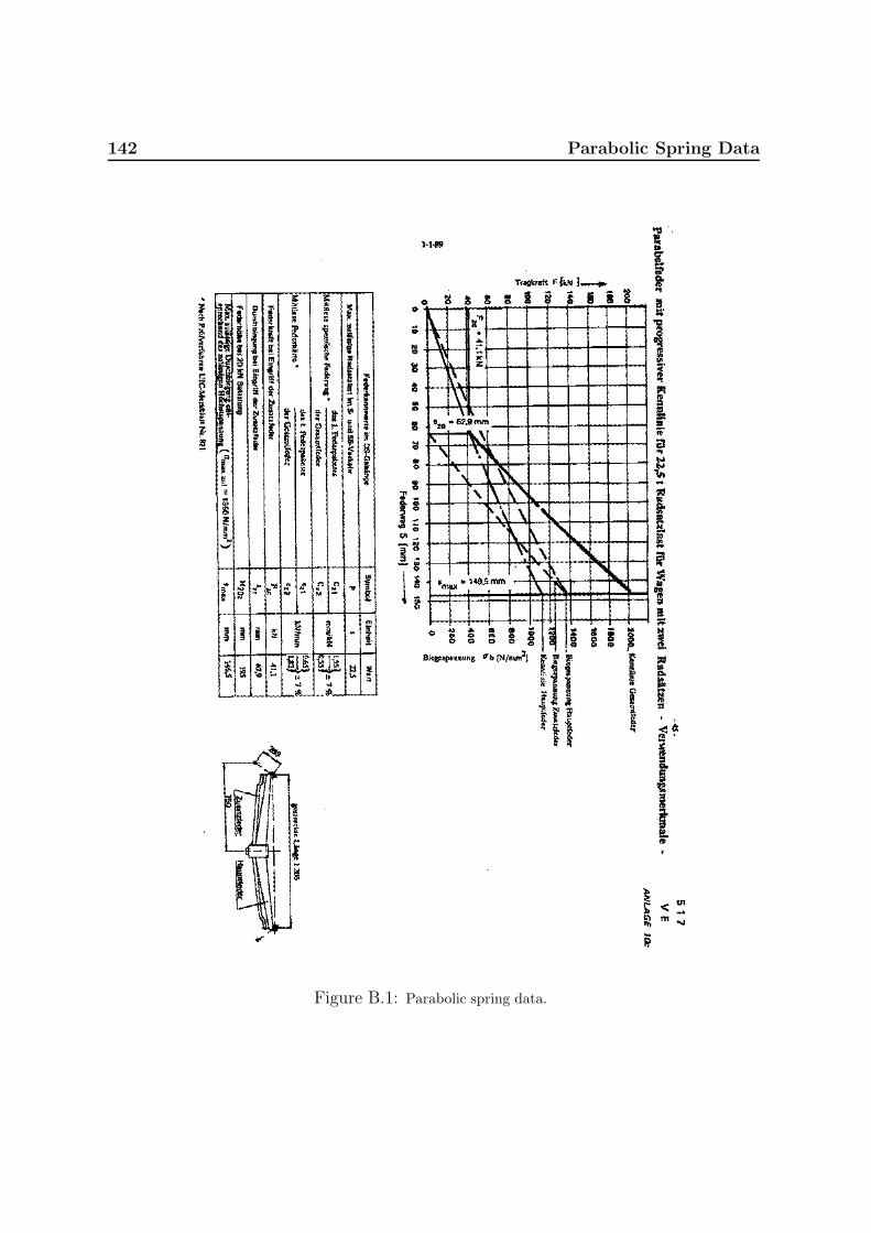
142 Parabolic Spring Data
Figure B.1: Parabolic spring data.

Appendix C
Coordinate Transformations
In this chapter we derive the transformation matrices which provide the connectionbetween the coordinate systems we use to describe the model. This is a matter ofchanging basis in a three dimensional Euclidean vector space.
Z’
Y’
Z
YX
X’φ
φ
LeftRight rr
r
Figure C.1: Rotate the angle φ around x.
Firstly, we find the transformation matrix between the rail coordinate system and thewheelset coordinate system. We rotate the rail coordinate system with the angle φaround its own x axis, and end up with the coordinate system denoted (X ′, Y ′, Z ′) (seefigure C.1). Let the canonical basis for the rail and (X ′, Y ′, Z ′) coordinate system be{erx, ery, erz} and {ex′ , ey′, ez′}, respectively. The matrix Mφ that switches rail coordi-nates to (X ′, Y ′, Z ′) coordinates is the coordinate matrix for {erx, ery, erz} with respectto the basis {ex′, ey′ , ez′}. Thus
ex =
1
00
ey =
0
cos φ− sinφ
ez =
0
sin φcosφ
i.e.
Mφ =
1 0 0
0 cosφ sin φ0 − sinφ cosφ

144 Coordinate Transformations
Yw
w
Xw
Left
Right
ψ
ψ
Z’X’
Y’
Z
Figure C.2: Rotation ψ around z′.
We now proceed by rotating the (X ′, Y ′, Z ′) coordinate system ψ around its own z′
axis and we end up with the wheelset coordinate system. The matrix that switches(X ′, Y ′, Z ′) coordinates to (Xw, Yw, Zw) coordinates is the coordinate matrix for {ex′,ey′ , ez′} with respect to the basis {ewx, ewy, ewz}.
ex =
cosψ
− sinψ0
ey =
sinψ
cosψ0
ez =
0
01
Thus
Mψ =
cosψ sinψ 0
− sinψ cosψ 00 0 1
The matrix that switches rail coordinates to wheelset coordinates is
wMr = Mψ · Mφ =
cosψ sinψ cosφ sinψ sinφ
− sinψ cosψ cos φ cosψ sin φ0 − sin φ cos φ
≈
1 ψ 0
−ψ 1 φ0 −φ 1
We now seek the transformation matrix that converts contact coordinates to wheelsetcoordinates and it is found in precisely the same manner as before (see figure C.3).For the left wheel the coordinate matrix for {ecx, ecy, ecz} with respect to the basis{ewx, ewy, ewz} is
ex =
1
00
ey =
0
cos δlsin δl
ez =
0
− sin δlcos δl
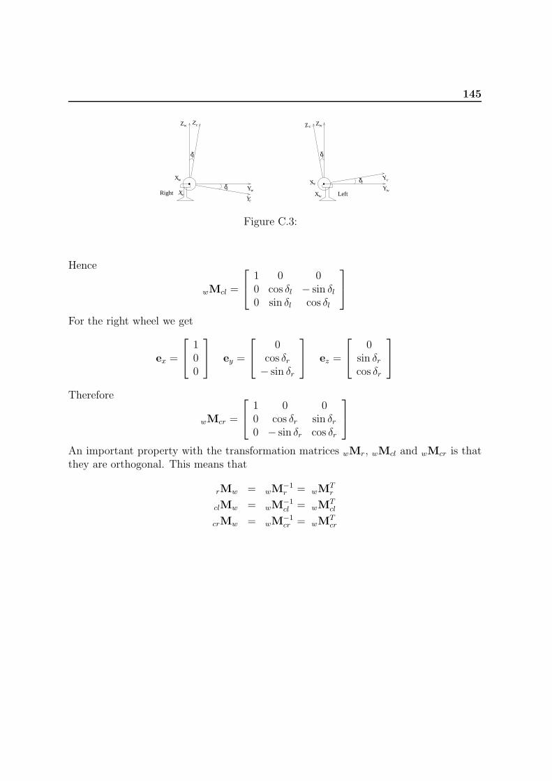
145
Left
c c
Xc
Zw
Yw
Xw c
Xw
Zw
RightY
Z
δ
δ
c
Xcr
r
Z
δ
δ
l
l
Y
Yw
Figure C.3:
Hence
wMcl =
1 0 0
0 cos δl − sin δl0 sin δl cos δl
For the right wheel we get
ex =
1
00
ey =
0
cos δr− sin δr
ez =
0
sin δrcos δr
Therefore
wMcr =
1 0 0
0 cos δr sin δr0 − sin δr cos δr
An important property with the transformation matrices wMr, wMcl and wMcr is thatthey are orthogonal. This means that
rMw = wM−1r = wM
Tr
clMw = wM−1cl = wM
Tcl
crMw = wM−1cr = wM
Tcr

146 Coordinate Transformations
We are also able to find the transformation matrices that converts contact coordinatesto rail coordinates and vice versa. We utilize the addition formulas and get
rMcl = rMw · wMcl
=
cosψ − sinψ 0
sinψ cosφ cosψ cosφ − sinφsinψ sin φ cosψ sin φ cos φ
· 1 0 0
0 cos δl − sin δl0 sin δl cos δl
≈ 1 −ψ cos δl ψ sin δlψ cos(δl + φ) − sin(δl + φ)0 sin(δl + φ) cos(δl + φ)
rMcr = rMw · wMcr
≈ 1 −ψ cos δr −ψ sin δrψ cos(δr − φ) sin(δr − φ)0 − sin(δr − φ) cos(δr − φ)
clMr = clMw · wMr
≈ 1 ψ 0
−ψ cos δl cos(δl + φ) sin(δl + φ)ψ sin δl − sin(δl + φ) cos(δl + φ)
crMr = crMw · wMr
≈ 1 ψ 0
−ψ cos δr cos(δr − φ) − sin(δr − φ)−ψ sin δr sin(δr − φ) cos(δr − φ)

147
A complete list of the rotational matrices used is presented below
bMr =
1 ψ 0
−ψ 1 φ0 −φ 1
(rail to car body)
wMr =
1 ψ 0
−ψ 1 φ0 −φ 1
(rail to wheelset)
rMw =
1 −ψ 0ψ 1 −φ0 φ 1
(wheelset to rail)
wMcl =
1 0 0
0 cos δl − sin δl0 sin δl cos δl
(contact left to wheelset)
wMcr =
1 0 0
0 cos δr sin δr0 − sin δr cos δr
(contact right to wheelset)
clMw =
1 0 0
0 cos δl sin δl0 − sin δl cos δl
(wheelset to contact left)
crMw =
1 0 0
0 cos δr − sin δr0 sin δr cos δr
(wheelset to contact right)
rMcl =
1 −ψ cos δl ψ sin δlψ cos(δl + φ) − sin(δl + φ)0 sin(δl + φ) cos(δl + φ)
(contact left to rail)
rMcr =
1 −ψ cos δr −ψ sin δrψ cos(δr − φ) sin(δr − φ)0 − sin(δr − φ) cos(δr − φ)
(contact right to rail)
clMr =
1 ψ 0
−ψ cos δl cos(δl + φ) sin(δl + φ)ψ sin δl − sin(δl + φ) cos(δl + φ)
(rail to contact left)
crMr =
1 ψ 0
−ψ cos δr cos(δr − φ) − sin(δr − φ)−ψ sin δr sin(δr − φ) cos(δr − φ)
(rail to contact right)

148 Coordinate Transformations

Appendix D
Creepage
In this chapter we will derive the velocity of the contact point relative to the rail. Forthis we use a new set of coordinate systems that are similar to the previously definedcoordinate systems, except that they are fixed in time. One could consider these newcoordinate systems as a snapshot of the original ones at a specific instance in time.We denote these new coordinate systems by (X ′
r, Y′r , Z
′r), (X ′
w, Y′w, Z
′w) and (X ′
c, Y′c , Z
′c).
The task is to find the velocity of the contact points in reference to (X ′c, Y
′c , Z
′c), i.e. the
velocity of the contact point relative to the rail.In general, the velocity of a point on a rigid body consist of two parts. Firstly,
there is a contribution due to the translational velocity of the body, and secondly, theangular velocity of the body. With respect to our problem we find that the velocity ofthe contact point is a composition of the translational velocity of the center of mass androtational velocity around the center point of the wheelset. Thus, the velocity of thecontact point is
Vc = Vtrans + Vrot
The translational velocity of the center of mass is
Vtrans = (V + x) · e′rx + y · e′
ry + z · e′rz
The rotational velocity around the center of mass is
Vrot = ω × r
where
ω = φ · e′wx + χ · e′
wy + ψ · e′wz
The vector from the center of mass of the wheelset to the contact point is
r =
{0 · e′
wx + al · e′wy − rl · e′
wz left contact point0 · e′
wx − ar · e′wy − rr · e′
wz right contact point

150 Creepage
In reference to (X ′w, Y
′w, Z
′w) we find regarding the left contact point
Vcl = wMr
V + x
yz
+
φχ
ψ
×
0
al
−rl
=
1 ψ 0
−ψ 1 φ0 −φ 1
V + x
yz
+
φχ
ψ
×
0
al
−rl
=
V + x+ ψy − rlχ− alψ
−ψ(V + x) + y + φz + rlφ
−φy + z + alφ
and for the right contact point the result is
Vcr =
V + x+ ψy − rrχ+ arψ
−ψ(V + x) + y + φz + rrφ
−φy + z − arφ
In reference to (X ′c, Y
′c , Z
′c) we now find
Vcl = clMw
V + x+ ψy − rlχ− alψ
−ψ(V + x) + y + φz + rlφ
−φy + z + alφ
=
1 0 0
0 cos δl sin δl0 − sin δl cos δl
V + x+ ψy − rlχ− alψ
−ψ(V + x) + y + φz + rlφ
−φy + z + alφ
=
V + x+ ψy − rlχ− alψ
(−ψ(V + x) + y + φz + rlφ) cos δl + (−φy + z + alφ) sin δl−(−ψ(V + x) + y + φz + rlφ) sin δl + (−φy + z + alφ) cos δl
≈ V + x− rlχ− alψ
(−ψV + y + rlφ) cos δl + (z + alφ) sin δl−(−ψV + y + rlφ) sin δl + (z + alφ) cos δl
and
Vcr = crMw
V + x+ ψy − rrχ+ arψ
−ψ(V + x) + y + φz + rrφ
−φy + z − arφ
=
1 0 0
0 cos δr − sin δr0 sin δr cos δr
V + x+ ψy − rrχ+ arψ
−ψ(V + x) + y + φz + rrφ
−φy + z − arφ
=
V + x+ ψy − rrχ+ arψ
(−ψ(V + x) + y + φz + rrφ) cos δr − (−φy + z − arφ) sin δr(−ψ(V + x) + y + φz + rrφ) sin δr + (−φy + z − arφ) cos δr
≈ V + x− rrχ+ arψ
(−ψV + y + rrφ) cos δr − (z − arφ) sin δr(−ψV + y + rrφ) sin δr + (z − arφ) cos δr

151
The longitudinal and lateral creep are defined by
ξlong =vlong,wheel − vlong,rail
V
ξlat =vlat,wheel − vlat,rail
VSince the rail is assumed to be fixed we find
ξlx = 1 − rlχ
V+x− alψ
V
ξrx = 1 − rrχ
V+x+ arψ
V
ξly =
(−ψ +
y + rlφ
V
)cos δl +
z + alφ
Vsin δl
ξry =
(−ψ +
y + rrφ
V
)cos δr − z − arφ
Vsin δr
where we have neglected second order terms.Finally, the spin creep terms are defined as the rotation around the normal to the
contact plane normalized by the velocity. First, we have to find the angular velocity ofthe wheelset in reference to (X ′
c, Y′c , Z
′c).
ωcl = clMw · ω
=
1 0 0
0 cos δl sin δl0 − sin δl cos δl
φχ
ψ
=
φ
χ cos δl + ψ sin δl−χ sin δl + ψ cos δl
ωcr = crMw · ω
=
1 0 0
0 cos δr − sin δr0 sin δr cos δr
φχ
ψ
=
φ
χ cos δr − ψ sin δrχ sin δr + ψ cos δr
Thus
ξls =−χ sin δl + ψ cos δl
V
ξrs =χ sin δr + ψ cos δr
V

152 Creepage

Appendix E
Additional Penetration
In this chapter we will derive the expressions we have used to calculate the additionalpenetration due to the roll and vertical motion of the wheelset. This additional penetra-tion combined with the static penetration from the RSGEO table enables us to computethe normal force dynamically.
Firstly, we find the vector from the contact point on the wheel to the contact pointon the rail (see Figure E.1 and E.2 for details). For the left wheel we get
Rr −Rw =
xRlaRlzRl
−
xyz
+ rMw ·
0
al−rl
=
xRl − xaRl − yzRl − z
−
1 −ψ 0ψ 1 −φ0 φ 1
· 0
al−rl
=
xRl − x+ ψalaRl − y − al − φrlzRl − z − φal + rl
We exclude the term zRl + rl because it is not a part of the additional penetration.Furthermore, we need to switch to the contact coordinate system, since the penetrationis the z-component of this.
∆P = clMr · xRl − x+ ψalaRl − y − al − φrl
−z − φal
=
1 ψ 0
−ψ cos δl cos(δl + φ) sin(δl + φ)ψ sin δl − sin(δl + φ) cos(δl + φ)
· xRl − x+ ψalaRl − y − al − φrl
−z − φal

154 Additional Penetration
The additional penetration is
∆Padd,l = ψ(xRl − x+ ψal) sin δl − (aRl − y − al − φrl) sin(δl + φ)
+(−z − φal) cos(δl + φ)
≈ −(aRl − y − al − φrl) sin(δl + φ) + (−z − φal) cos(δl + φ)
We follow the same procedure for the right wheel and we get
Rr −Rw =
xRr
−aRrzRr
−
xyz
+ rMw ·
0
−ar−rr
=
xRr − x
−aRr − yzRr − y
−
1 −ψ 0ψ 1 −φ0 φ 1
· 0
−ar−rr
=
xRr − x− ψar
−aRr − y + ar − φrrzRr − z + φar + rr
∆P = crMr · xRr − x− ψar
−aRr − y + ar − φrr−z + φar
=
1 ψ 0
−ψ cos δr cos(δr − φ) − sin(δr − φ)−ψ sin δr sin(δr − φ) cos(δr − φ)
· xRr − x− ψar
−aRr − y + ar − φrr−z + φar
The additional penetration is
∆Padd,r = −ψ(xRr − x− ψar) sin δr + (−aRr − y + ar − φrr) sin(δr − φ)
+(−z + φar) cos(δr − φ)
≈ (−aRr − y + ar − φrr) sin(δr − φ) + (−z + φar) cos(δr − φ)

155
z
yx
aRlaRr
Rr−z Rl−z
Rail coordinate system
Contact point on the rail
Figure E.1:
z
yx
ar al
r lr r
Wheel coordinate system
Contact point on the wheel
Figure E.2:

156 Additional Penetration

Appendix F
Differential Succesion of the DryFriction Element
k1T0
y
Figure F.1: Dry friction element.
We consider the dry friction element shown in figure F.1. The continuity conditionfor this element is
T = k1(−y − vs) (F.1)
The restoring force is bounded by Coulomb friction law, which is illustrated in figure F.2.It is important to know that this figure does not represent a mathematical function. Dueto the non smooth characteristic of the friction force we make a differential succesion inorder to improve the numerical solution process.
For |T | < T0 the sliding velocity of the dry friction slider is zero, which means that
T = −k1y |T | < T0
For T = T0 we have the situation shown in figure F.3. We have multiplied vs by anarbitrary real number ρ, which is to be determined later on. This non smooth functionis parameteries by the parameter s as illustrated in the figure. This leads to
T =
{0 s ≥ 0s s < 0
ρvs =
{s s ≥ 00 s < 0
By adding these two equations we find that
T + ρvs = s

158 Differential Succesion of the Dry Friction Element
and according to the previous equation for T we see that
T = [s]− = −[−s]+ = −[−T − ρvs]+ T = T0 (F.2)
where
[x]+ =
{x x ≥ 00 x < 0
[x]− =
{0 x ≥ 0x x < 0
By substituting the sliding velocity of the dry friction slider from equation (F.1) into(F.2) we get
T = −[−T − ρ
[−y − T
k1
]]+
T = T0
by choosing ρ = k1 we see that
T = − [k1y]+ T = T0
Similary, we have for T = −T0 (see figure F.4)
T =
{s s ≥ 00 s < 0
ρvs =
{0 s ≥ 0s s < 0
thusT + ρvs = s
and according to the previous equation for T we see that
T = [s]+ =
[T + ρ
[−y − T
k1
]]+
= [−k1y]+ T = −T0
Thus, we have found that
T =
−k1y |T | < T0
− [k1y]+ T = T0
[−k1y]+ T = −T0

159
(a)
- vs
6
T
T0
−T0
(b)
Figure F.2: (a) Measurement on clean surfaces confirming that the dry friction force obeys Coulomb’sfriction relation. (b) Schematic diagram of Coulombs friction relation. It is not a mathematical function.

160 Differential Succesion of the Dry Friction Element
- ρvs
6
T
� - s
@@
s = 0 s > 0
s < 0
Figure F.3: T = T0
- ρvs
6
T
�
6s
@@s = 0
s > 0
s < 0
Figure F.4: T = −T0

Appendix G
Maple Code for the Calculations ofthe Moment of Inertia
Our model of the car body consists of the following elements:
(1) Underframe (6395 kg)(1) Floor (662 kg)(2) Front wall (550 kg each)(1) Roof (1339 kg)(4) Partition (244 kg each)(2) Sliding panels (1024 kg each)(4) buffer (149 kg each)(1) Center column (183 kg)(2) rail for sliding panels (132 kg each)
Total mass is 13563 kg
> restart;
> d1 := 0.6525; d2 := 1.595; d3 := 0.265; d4 := 2.350; d5 := 0.865; d6> := sqrt(d1^2+d5^2); d7 := d1/2; d8 := 16.01; d9 := 2*d1 + d2;
d1 := .6525
d2 := 1.595
d3 := .265
d4 := 2.350
d5 := .865
d6 := 1.083504153
d7 := .3262500000
d8 := 16.01
d9 := 2.9000
> A_underframe := d8*(2*d1+d2); A_floor := A_underframe; A_frontwall :=> 2*d1*d4 + d1*d5 + d2*(d4+d5); A_roof1 := d6*d8; A_roof2 := d2*d8;> A_roof3 := A_roof1; A_roof := A_roof1 + A_roof2 + A_roof3; A_partition> := A_frontwall; A_slidingpanels := d8*d4; l_cencol := d2+2*d4+2*d6;> l_cencol1 := d4; l_cencol2 := d6; l_cencol3 := d2;
A underframe := 46.429000
A floor := 46.429000
A frontwall := 8.7590875
A roof1 := 17.34690149
A roof2 := 25.53595
A roof3 := 17.34690149
A roof := 60.22975298
A partition := 8.7590875

162 Maple Code for the Calculations of the Moment of Inertia
A slidingpanels := 37.62350
l cencol := 8.462008306
l cencol1 := 2.350
l cencol2 := 1.083504153
l cencol3 := 1.595> M_underframe := 6395; M_floor := 662; M_frontwall := 550; M_roof :=> 1339; M_roof1 := A_roof1/A_roof*M_roof; M_roof2 :=> A_roof2/A_roof*M_roof; M_roof3 := M_roof1; M_partition := 244;> M_slidingpanels := 1024; M_buffer := 149; M_cencol := 183; M_cencol1> := l_cencol1/l_cencol*M_cencol; M_cencol2 :=> l_cencol2/l_cencol*M_cencol; M_cencol3 := l_cencol3/l_cencol*M_cencol;> M_rail := 132; M_carbody := M_underframe + M_floor + 2*M_frontwall +> M_roof + 4*M_partition + 2*M_slidingpanels + 4*M_buffer + M_cencol +> 2*M_rail;
M underframe := 6395
M floor := 662
M frontwall := 550
M roof := 1339
M roof1 := 385.6482876
M roof2 := 567.7034249
M roof3 := 385.6482876
M partition := 244
M slidingpanels := 1024
M buffer := 149
M cencol := 183
M cencol1 := 50.82126895
M cencol2 := 23.43193870
M cencol3 := 34.49358467
M rail := 132
M carbody := 13563
Center of mass calculations of our model of the car body
Underframe
> r_cz_underframe := 0;
r cz underframe := 0
Floor
> r_cz_floor := d3;
r cz floor := .265
Front wall
> r_cz_frontwall_int1 := int(int(z,z=d3..d3+d4+d5/d1*y),y=0..d1):
> r_cz_frontwall_int2 := int(int(z,z=d3..d3+d4+d5),y=d1..d1+d2):
> r_cz_frontwall_int3 :=> int(int(z,z=d3..d3+d4+d5-d5/d1*(y-d1-d2)),y=d1+d2..2*d1+d2):
> r_cz_frontwall := simplify(1/A_frontwall*(r_cz_frontwall_int1 +> r_cz_frontwall_int2 + r_cz_frontwall_int3));
r cz frontwall := 1.787496379
Roof
> r_cz_roof := simplify(1/M_roof*(M_roof1*(d3+d4+d5/2) +> M_roof2*(d3+d4+d5) + M_roof3*(d3+d4+d5/2)));
r cz roof := 3.230869478

163
Partition
> r_cz_partition_int1 := int(int(z,z=d3..d3+d4+d5/d1*y),y=0..d1):
> r_cz_partition_int2 := int(int(z,z=d3..d3+d4+d5),y=d1..d1+d2):
> r_cz_partition_int3 :=> int(int(z,z=d3..d3+d4+d5-d5/d1*(y-d1-d2)),y=d1+d2..2*d1+d2):
> r_cz_partition := simplify(1/A_partition*(r_cz_partition_int1 +> r_cz_partition_int2 + r_cz_partition_int3));
r cz partition := 1.787496379
Sliding panels
> r_cz_slidingpanels := d3+d4/2;
r cz slidingpanels := 1.440000000
Buffers
> r_cz_buffer := d3;
r cz buffer := .265
Center column
r c = sum {i=1}ˆ{N}(m i*r i)/M total = sum {i=1}ˆ{N}(L i*r i)/L total
> r_cz_cencol := (2*M_cencol1*(d3+d4/2) + 2*M_cencol2*(d3+d4+d5/2) +> M_cencol3*(d3+d4+d5))/M_cencol;
r cz cencol := 2.236178119
Rails for sliding panels
> r_cz_rail := d3+d4;
r cz rail := 2.615
Car body
Due to symmetry we have
> r_cx_carbody := d8/2;
r cx carbody := 8.005000000
Due to symmetry we have
> r_cy_carbody := d1 + d2/2;
r cy carbody := 1.450000000
r c = sum {i=1}ˆ{N}(m i*r i)/M total
> r_cz_carbody := simplify(1/M_carbody*(M_underframe*r_cz_underframe +> M_floor*r_cz_floor + 2*M_frontwall*r_cz_frontwall + M_roof*r_cz_roof +> 4*M_partition*r_cz_partition + 4*M_partition*r_cz_slidingpanels +> 4*M_buffer*r_cz_buffer + M_cencol*r_cz_cencol +> 2*M_rail*r_cz_rail));
r cz carbody := .8018408398
Adding freight
> M_freight := 20000:
> rho_freight := 19300:
> h_freight := M_freight/(rho_freight*d8*d9);
h freight := .02231944323
> r_cz_freight := h_freight/2 + d3:
> r_cz_carbody := (M_carbody*r_cz_carbody +> M_freight*r_cz_freight)/(M_carbody+M_freight);
r cz carbody := .4885904639
Moment of inertia calculations of our model of the car body
Underframe

164 Maple Code for the Calculations of the Moment of Inertia
Around a horizontal line through the center of mass of the underframe
> I_c_l1_underframe := 1/12*M_underframe*(2*d1+d2)^2;
I c l1 underframe := 4481.829167
Around a horizontal line through the center of mass of the car body
> I_l1_underframe := I_c_l1_underframe +> M_underframe*(r_cz_carbody-r_cz_underframe)^2;
I l1 underframe := 6008.447669
Around a vertical line through the center of mass of the underframe
> I_c_l2_underframe := 1/12*M_underframe*((2*d1+d2)^2+d8^2);
I c l2 underframe := 141079.0825
Around a vertical line through the center of mass of the car body
> I_l2_underframe := I_c_l2_underframe + M_underframe*0^2;
I l2 underframe := 141079.0825
Floor
Around a horizontal line through the center of mass of the floor
> I_c_l1_floor := 1/12*M_floor*(2*d1+d2)^2;
I c l1 floor := 463.9516667
Around a horizontal line through the center of mass of the car body
> I_l1_floor := I_c_l1_floor + M_floor*(r_cz_carbody-r_cz_floor)^2;
I l1 floor := 497.0468312
Around a vertical line through the center of mass of the floor
> I_c_l2_floor := 1/12*M_floor*((2*d1+d2)^2+d8^2);
I c l2 floor := 14604.27718
Around a vertical line through the center of mass of the car body
> I_l2_floor := I_c_l2_floor + M_floor*0^2;
I l2 floor := 14604.27718
Front wall
> integrand_frontwall_l1 := (r_cy_carbody-y)^2 + (r_cz_carbody-z)^2:
> I_l1_frontwall_int1 :=> int(int(integrand_frontwall_l1,z=d3..d3+d4+d5/d1*y),y=0..d1):
> I_l1_frontwall_int2 :=> int(int(integrand_frontwall_l1,z=d3..d3+d4+d5),y=d1..d1+d2):
> I_l1_frontwall_int3 :=> int(int(integrand_frontwall_l1,z=d3..d3+d4+d5-d5/d1*(y-d1-d2)),y=d1+d2> ..2*d1+d2):
Around a horizontal line (parallel to the track ) through the center of mass of the car body
> I_l1_frontwall := M_frontwall/A_frontwall*(I_l1_frontwall_int1 +> I_l1_frontwall_int2 + I_l1_frontwall_int3);
I l1 frontwall := 1720.707385
> integrand_frontwall_l2 := (r_cy_carbody-y)^2:
> I_l2_frontwall_int1 :=> int(int(integrand_frontwall_l2,z=d3..d3+d4+d5/d1*y),y=0..d1):
> I_l2_frontwall_int2 :=> int(int(integrand_frontwall_l2,z=d3..d3+d4+d5),y=d1..d1+d2):
> I_l2_frontwall_int3 :=> int(int(integrand_frontwall_l2,z=d3..d3+d4+d5-d5/d1*(y-d1-d2)),y=d1+d2> ..2*d1+d2):
Around a vertical line through the center of mass of the front wall
> I_c_l2_frontwall := M_frontwall/A_frontwall*(I_l2_frontwall_int1 +> I_l2_frontwall_int2 + I_l2_frontwall_int3);
I c l2 frontwall := 355.6217837
Around a vertical line through the center of mass of the car body
> I_l2_frontwall := I_c_l2_frontwall + M_frontwall*(d8/2)^2;
I l2 frontwall := 35599.63553
Roof

165
Roof 1Around a horizontal line through the center of mass of roof 1
> I_c_l1_roof1 := 1/12*M_roof1*d6^2:
Around a horizontal line through the center of mass of the car body
> I_l1_roof1 := I_c_l1_roof1 +> M_roof1*((d1/2+d2/2)^2+(d3+d4+d5/2-r_cz_carbody)^2):
Roof 2Around a horizontal line through the center of mass of roof 2
> I_c_l1_roof2 := 1/12*M_roof2*d2^2:
Around a horizontal line through the center of mass of the car body
> I_l1_roof2 := I_c_l1_roof2 + M_roof2*(d3+d4+d5-r_cz_carbody)^2:
Roof 3Around a horizontal line through the center of mass of the car body
> I_l1_roof3 := I_l1_roof1:
Roof
> I_l1_roof := I_l1_roof1 + I_l1_roof2 + I_l1_roof3;
I l1 roof := 11300.39135
Roof 1Around a vertical line through the center of mass of roof 1
> I_c_l2_roof1 := 1/12*M_roof1*(d8^2+d1^2):
Around a vertical line through the center of mass of the car body
> I_l2_roof1 := I_c_l2_roof1 + M_roof1*(d1/2+d2/2)^2:
Roof 2Around a vertical line through the center of mass of roof 2
> I_c_l2_roof2 := 1/12*M_roof2*(d8^2+d2^2):
Around a vertical line through the center of mass of the car body
> I_l2_roof2 := I_c_l2_roof2 + M_roof2*0^2:
Roof 3Around a vertical line through the center of mass of the car body
> I_l2_roof3 := I_l2_roof1:
Roof
> I_l2_roof := I_l2_roof1 + I_l2_roof2 + I_l2_roof3;
I l2 roof := 29722.77499
Partition
> integrand_partition_l1 := (r_cy_carbody-y)^2 + (r_cz_carbody-z)^2:
> I_l1_partition_int1 :=> int(int(integrand_partition_l1,z=d3..d3+d4+d5/d1*y),y=0..d1):
> I_l1_partition_int2 :=> int(int(integrand_partition_l1,z=d3..d3+d4+d5),y=d1..d1+d2):
> I_l1_partition_int3 :=> int(int(integrand_partition_l1,z=d3..d3+d4+d5-d5/d1*(y-d1-d2)),y=d1+d2> ..2*d1+d2):
Around a horizontal line (parallel to the track ) through the center of mass of the car body
> I_l1_partition := M_partition/A_partition*(I_l1_partition_int1 +> I_l1_partition_int2 + I_l1_partition_int3);
I l1 partition := 763.3683674
> integrand_partition_l2 := (r_cy_carbody-y)^2:
> I_l2_partition_int1 :=> int(int(integrand_partition_l2,z=d3..d3+d4+d5/d1*y),y=0..d1):
> I_l2_partition_int2 :=> int(int(integrand_partition_l2,z=d3..d3+d4+d5),y=d1..d1+d2):
> I_l2_partition_int3 :=> int(int(integrand_partition_l2,z=d3..d3+d4+d5-d5/d1*(y-d1-d2)),y=d1+d2> ..2*d1+d2):
Around a vertical line through the center of mass of the partition
> I_c_l2_partition := M_partition/A_partition*(I_l2_partition_int1 +> I_l2_partition_int2 + I_l2_partition_int3);
I c l2 partition := 157.7667550
Around a vertical line through the center of mass of the car body
> I_l2_partition := I_c_l2_partition + M_partition*(d8/2)^2;
I l2 partition := 15793.29286

166 Maple Code for the Calculations of the Moment of Inertia
Sliding panels
Around a horizontal line through the center of mass of the sliding panels
> I_c_l1_slidingpanels := 1/12*M_slidingpanels*d4^2;
I c l1 slidingpanels := 471.2533333
Around a horizontal line through the center of mass of the car body
> I_l1_slidingpanels := I_c_l1_slidingpanels +> M_slidingpanels*((r_cy_carbody)^2+(r_cz_slidingpanels-r_cz_carbody)^2)> ;
I l1 slidingpanels := 3551.117761
Around a vertical line through the center of mass of the sliding panels
> I_c_l2_slidingpanels := 1/12*M_slidingpanels*d8^2;
I c l2 slidingpanels := 21872.64853
Around a vertical line through the center of mass of the car body
> I_l2_slidingpanels := I_c_l2_slidingpanels +> M_slidingpanels*(r_cy_carbody)^2;
I l2 slidingpanels := 24025.60853
Buffers
Around a horizontal line through the center of mass of the car body
> I_l1_buffer :=> M_buffer*((d1+d2/2-d7)^2+(r_cz_buffer-r_cz_carbody)^2);
I l1 buffer := 195.6082069
Around a vertical line through the center of mass of the car body
> I_l2_buffer := M_buffer*((d1+d2/2-d7)^2+(d8/2)^2);
I l2 buffer := 9736.083020
Center column
cencol 1Around a horizontal line through the center of mass of cencol1
> I_c_l1_cencol1 := 1/12*M_cencol1*d4^2:
Around a horizontal line through the center of mass of the car body
> I_l1_cencol1 := I_c_l1_cencol1 +> M_cencol1*((d1+d2/2)^2+(d3+d4/2-r_cz_carbody)^2):
cencol2Around a horizontal line through the center of mass of cencol2
> I_c_l1_cencol2 := 1/12*M_cencol2*d6^2:
Around a horizontal line through the center of mass of the car body
> I_l1_cencol2 := I_c_l1_cencol2 +> M_cencol2*((d1/2+d2/2)^2+(d3+d4+d5/2-r_cz_carbody)^2):
cencol3Around a horizontal line through the center of mass of cencol3
> I_c_l1_cencol3 := 1/12*M_cencol3*d2^2:
Around a horizontal line through the center of mass of the car body
> I_l1_cencol3 := I_c_l1_cencol3 +> M_cencol3*(d3+d4+d5-r_cz_carbody)^2:
center column
Around a horizontal line through the center of mass of the car body
> I_l1_cencol := 2*I_l1_cencol1 + 2*I_l1_cencol2 + I_l1_cencol3;
I l1 cencol := 1039.095259
cencol 1Around a vertical line through the center of mass of the car body
> I_l2_cencol2 := M_cencol1*(d1+d2/2)^2:
cencol2Around a vertical line through the center of mass of cencol2

167
> I_c_l2_cencol2 := 1/12*M_cencol2*d1^2:
Around a vertical line through the center of mass of the car body
> I_l2_cencol2 := I_c_l2_cencol2 + M_cencol2*(d1/2+d2/2)^2:
cencol3Around a vertical line through the center of mass of cencol3
> I_c_l2_cencol3 := 1/12*M_cencol3*d2^2:
Around a vertical line through the center of mass of the car body
> I_l2_cencol3 := I_c_l2_cencol3:
center column
Around a vertical line through the center of mass of the car body
> I_l2_cencol := 2*I_l2_cencol2 + 2*I_l2_cencol2 + I_l2_cencol3;
I l2 cencol := 128.9988700
Rail for sliding panels
Around a horizontal line through the center of mass of the car body
> I_l1_rail := M_rail*((d1+d2/2)^2+(d3+d4-r_cz_carbody)^2);
I l1 rail := 874.3835120
Around a vertical line through the center of mass of the rail
> I_c_l2_rail := 1/12*M_rail*d8^2:
Around a vertical line through the center of mass of the car body
> I_l2_rail := I_c_l2_rail + M_rail*(d1+d2/2)^2;
I l2 rail := 3097.051100
Car body
Around a horizontal line through the center of mass of the car body
> I_l1_carbody := I_l1_underframe + I_l1_floor + 2*I_l1_frontwall +> I_l1_roof + 4*I_l1_partition + 2*I_l1_slidingpanels + 4*I_l1_buffer +> I_l1_cencol + 2*I_l1_rail;
I l1 carbody := 34973.30472
Around a vertical line through the center of mass of the car body
> I_l2_carbody := I_l2_underframe + I_l2_floor + 2*I_l2_frontwall +> I_l2_roof + 4*I_l2_partition + 2*I_l2_slidingpanels + 4*I_l2_buffer +> I_l2_cencol + 2*I_l2_rail;
I l2 carbody := 413097.2275
Adding freight
> I_l1_carbody := I_l1_carbody + 1/12*M_freight*(d9^2+h_freight^2) +> M_freight*(r_cz_carbody - r_cz_freight)^2;
I l1 carbody := 49893.33806
> I_l2_carbody := I_l2_carbody + 1/12*M_freight*(d8^2+d9^2);
I l2 carbody := 854314.0608
> r_cx_carbody; r_cy_carbody; r_cz_carbody;
8.005000000
1.450000000
.4885904639

168 Maple Code for the Calculations of the Moment of Inertia

Appendix H
RSGEO table
The data table known as the RSGEO table is of central importance to our simulations inthat it stipulates important contact parameters related to the wheel-rail interface. Thistable, tabulated with respect to lateral motion of a wheelset, was created by Walter Kikfor Lasse Engbo Christiansen, and used in [4]. In this chapter, we present a series offigures which demonstrate how important parameters in the wheel-rail interface changewith shifting lateral movement of a wheelset. Importantly, all values were generated fora wheelset with S1002 profile wheels resting under its own weight on UIC60 rails, cantedat 1/40 towards the centerline for a track with a gauge of 1435 mm. Furthermore, thetable is for the left wheel only, and we assume symmetry with respect to the right wheel.

170 RSGEO table
−0.02 −0.015 −0.01 −0.005 0 0.005 0.01 0.015 0.023
4
5
6
7
8
9
10
11
12
13
Displacement of wheelset [m]
C11
Kalker’s creepage coefficient C11 vs. displacement of the wheelset
(a) Kalker’s creepage coefficientC11.
−0.02 −0.015 −0.01 −0.005 0 0.005 0.01 0.015 0.022
4
6
8
10
12
14
16
Displacement of wheelset [m]
C22
Kalker’s creepage coefficient C22 vs. displacement of the wheelset
(b) Kalker’s creepage coefficientC22.
−0.02 −0.015 −0.01 −0.005 0 0.005 0.01 0.015 0.020
2
4
6
8
10
12
14
16
18
Displacement of wheelset [m]
C23
Kalker’s creepage coefficient C23 vs. displacement of the wheelset
(c) Kalker’s creepage coefficientC23.
−0.02 −0.015 −0.01 −0.005 0 0.005 0.01 0.015 0.020
0.2
0.4
0.6
0.8
1
1.2
1.4
Displacement of wheelset [m]
Con
tact
ang
le [r
ad]
Contact angle vs. displacement of the wheelset
(d) Contact angle.
−0.02 −0.015 −0.01 −0.005 0 0.005 0.01 0.015 0.020
0.002
0.004
0.006
0.008
0.01
0.012
Displacement of wheelset [m]
Mag
nitu
de o
f sem
i axi
s [m
]
Size of contact ellipse
Longitudinal directionLateral direction
(e) Semi axes in contact ellipse.
−0.02 −0.015 −0.01 −0.005 0 0.005 0.01 0.015 0.020.69
0.7
0.71
0.72
0.73
0.74
0.75
0.76
0.77
0.78
Displacement of wheelset [m]
Dis
tanc
e [m
]
Lateral distance to contact point vs. displacement of the wheelset
(f) Lateral distance to the contactpoint on the wheel.
Figure H.1: RSGEO table (left wheel).

171
−0.02 −0.015 −0.01 −0.005 0 0.005 0.01 0.015 0.02
0.72
0.73
0.74
0.75
0.76
Displacement of wheelset [m]
Dis
tanc
e [m
]
Lateral distance to the contact point on the rail vs. displacement of the wheelset
(a) Lateral distance to the con-tact point on the rail.
−0.02 −0.015 −0.01 −0.005 0 0.005 0.01 0.015 0.020.42
0.425
0.43
0.435
0.44
0.445
0.45
0.455
Displacement of wheelset [m]
Rol
ling
radi
us [m
]
Rolling radius vs. displacement of the wheelset
(b) Wheel rolling radius.
−0.02 −0.015 −0.01 −0.005 0 0.005 0.01 0.015 0.022
2.5
3
3.5
4
4.5
5
5.5
6
6.5
7x 10
4
Displacement of wheelset [m]
Sta
tic n
orm
al fo
rce
[N]
Static normal force vs. displacement of the wheelset
(c) Static normal force.
−0.02 −0.015 −0.01 −0.005 0 0.005 0.01 0.015 0.025
6
7
8
9
10
11
12x 10
−5
Displacement of wheelset [m]
Sta
tic p
enet
ratio
n [m
]
Static penetration vs. displacement of the wheelset
(d) Static penetration.
−0.02 −0.015 −0.01 −0.005 0 0.005 0.01 0.015 0.02−0.012
−0.01
−0.008
−0.006
−0.004
−0.002
0
Displacement of wheelset [m]
Ver
tical
pos
ition
of c
onta
ct p
oint
[m]
Vertical position of contact point on the rail vs. displacement of the wheelset
(e) Vertical position of the con-tact point on the rail.
Figure H.2: RSGEO table (left wheel).

172 RSGEO table

Appendix I
Java Demonstration
We here present a series of figures which illustrate the Java based GUI for the C++ codethat implements our simulation model. As this is true cross platform code, we haveshown screenshots for both Sun’s Solaris as used by IMM1, as well as Apple’s FreeBSDUNIX based Mac OS X.2.6.
I.1 Sun Solaris 5.8
The figures presented in this section were produced under Sun’s Solaris 5.8 which is usedat IMM and a greater part of DTU.
1Institute for Informatics and Mathematical Modelling

174 Java Demonstration
Figure I.1: Main program window under Solaris.

I.1 Sun Solaris 5.8 175
Figure I.2: Simulation output under Solaris.

176 Java Demonstration
Figure I.3: Choosing a saved simulation file under Solaris.
Figure I.4: Choosing what to plot under Solaris.

I.1 Sun Solaris 5.8 177
Figure I.5: Choosing linear suspension parameters under Solaris.
Figure I.6: Choosing progressive spring suspension parameters under Solaris.

178 Java Demonstration
Figure I.7: Choosing standard leaf spring suspension parameters under Solaris.

I.2 Apple Mac OS X.2.6 Jaguar 179
I.2 Apple Mac OS X.2.6 Jaguar
The figures presented in this section were produced under Apple’s Mac OS X.2.6.
Figure I.8: Main program window under Mac OS X.

180 Java Demonstration
Figure I.9: Simulation output under Mac OS X.

I.2 Apple Mac OS X.2.6 Jaguar 181
Figure I.10: Choosing a saved simulation file under Mac OS X.
Figure I.11: Choosing what to plot under Mac OS X.
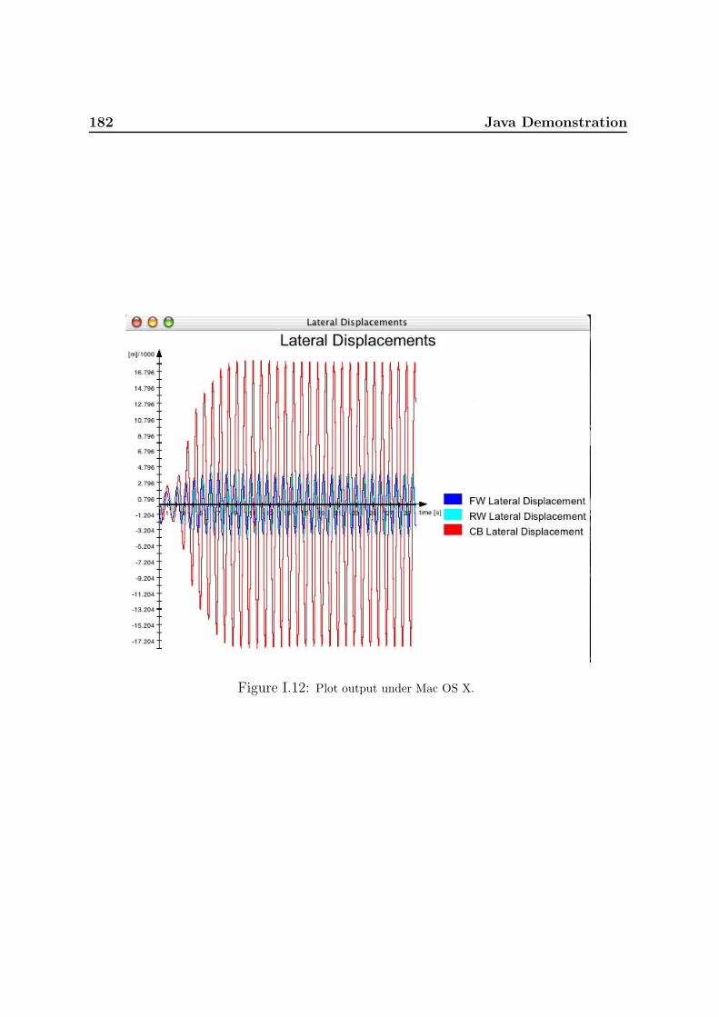
182 Java Demonstration
Figure I.12: Plot output under Mac OS X.

Bibliography
[1] Barbara Blazejczyk-Okolewska, Krzysztof Czolczynski, Tomasz Kapitaniak, andJerzy Wojewoda. Chaotic Mechanics in Systems with Impacts and Friction, vol-ume 36 of A. World Scientific, 1999.
[2] David Cebon. Handbook of Vehicle-Road Interaction. Swets & Zeitlinger.
[3] Gunnar Christensen, Erik Both, and Preben Østergaard Sørensen. Mekanik (inDanish). Scantryk A/S, 1997.
[4] Lasse Engbo Christiansen. The Dynamics of a Railway Vehicle on a DisturbedTrack. Master’s thesis, Technical University of Denmark, June 2001.
[5] Vijay K. Garg and Rao V. Dukkipati. Dynamics of Railway Vehicle Systems.Academic Press, 1984.
[6] Wolfgang Hanneforth and Werner Fischer. Laufwerke (in German). transpressVEB Verlag fur Verkehrswesen, 1986.
[7] Jens Christian Jensen. Teoretiske og eksperimentelle dynamiske undersøgelser afjernbanekøretøjer (in Danish). PhD thesis, IMM-DTU, 1995.
[8] Jerzy Piotrowski. A Mathematical Model of the UIC Link Suspension for FreightWagons. Technical report, Institute of Vehicles, Warsaw University of Technology.
[9] Eva Charlotte Slivsgaard. On the Interaction Between Wheels and Rails in RailwayDynamics. PhD thesis, IMM-DTU, 1995.
[10] Steven H. Strogatz. Nonlinear Dynamics and Chaos. Perseus Books, 8 edition,1998.
[11] Henrik Thillman. Non-Linear Railway Vehicle Dynamics. Master’s thesis, TechnicalUniversity of Denmark, July 2000.
[12] Lars Trzepacz. Railway Freight Vehicle Dynamics. Master’s thesis, Technical Uni-versity of Denmark, July 2002.