Droplet Interactions during Combustion of Unsupported Droplet Clusters

In Microgravity:

Numerical Study of Droplet Interactions at Low Reynolds Number

A Thesis

Submitted to the Faculty

of

Drexel University

by

Irina N. Ciobanescu Husanu

in partial fulfillment of the

requirements for the degree

of

Doctor of Philosophy

December 2005

©Copyright 2005

Irina N. Ciobanescu Husanu. All Rights Reserved.

ii

DEDICATIONS

In the memory of my father,

Dedicated professor Dr. Mihail-Serban Voiculescu, whose life and career were my role models

for each moment of my life. His unconditional love and his continuing support and care were, are,

and will ever be my guiding light, even if now is watching over me from Heaven. You will be

forever alive in my heart.

To my mother,

Dr. Doina Voiculescu, a wonderful doctor and professor and loving and devoted mother, for

always encouraging me to pursue academic success. You always have been the shoulder to lean

on or to cry on, and your courage, determination and creativity motivated me to keep going

forward.

iii

ACKNOWLEDGEMENTS

I would like to express my deep gratitude to my advisors Dr. Gary A. Ruff and

Dr. Mun Y. Choi for their guidance and assistance throughout the duration of this

research. Their encouragement and support were critical to the success of this project. I

would like to extend my special thanks to Dr. Ruff, who always was there for me when I

needed and whose valuable advice and suggestions helped me performing the research.

I would like to thank all of my committee members, including Dr. Gary A.Ruff,

Dr. Mun Y. Choi, Dr. Nicholas Cernansky, Dr.Howard Pearlman, Dr. Alan Lau, and Dr.

Alexander Dolgopolsky for encouraging me and offering precious suggestions and

feedback.

My special appreciation is extended to NIST team for publicly releasing the Fire

Dynamic Simulator code that was of tremendous help in developing the present

investigation, along with their continuous support every time I needed.

Special thanks go to NASA Drop Tower and Microgravity Combustion Research

Laboratory teams from NASA Glenn Research Center, for their help and support in

design and fabrication of the equipment as well as for their important suggestions and

advice.

I am exceptionally grateful to my family, my husband, my daughters and my

stepson for their remarkable patience, encouragements and for always believing in me.

Special appreciation to my daughters Ana and Diana for their contribution to data

collection for my research, and for cooking for our entire family while I was researching.

iv

The support of the NASA Office of Biological and Physical Research,

Microgravity Combustion Research Program (Grant Number NCC3-847) is greatly

appreciated.

All my thanks to those who helped, encouraged and supported me during these

past years and whose names are not mentioned here, to all my friends and relatives.

v

TABLE OF CONTENTS

Page

LIST OF TABLES........................................................................................................................viii

LIST OF FIGURES ......................................................................................................................... x

ABSTRACT................................................................................................................................... xv

CHAPTER 1: INTRODUCTION .................................................................................................... 1

CHAPTER 2: BACKGROUND ...................................................................................................... 4

2.1 Studies of Single and Multi-Component Isolated Droplets....................................... 4

2.2 Studies of Arrays of Droplets and Streams ............................................................. 11

2.2.1 Theoretical Analysis ..................................................................................................... 11

2.2.2 Experiments Involving Arrays of Drops....................................................................... 17

2.2.3 Radiative Heat Loss Studies on Fuel Droplet Combustion........................................... 19

2.3 Summary ................................................................................................................. 20

CHAPTER 3: DROPLET INTERACTIONS AT LOW REYNOLDS NUMBERS ..................... 23

3.1 Point Source Method............................................................................................... 23

3.1.1 Description of the Method ............................................................................................ 23

3.1.2 Advantages and Disadvantages of the Method ............................................................. 26

3.2. Extension of the PSM for Non-symmetric Arrays ................................................. 29

3.2.1 Method Description ...................................................................................................... 30

3.2.2 Results of the PSM for Non-symmetric Arrays ............................................................ 31

vi

CHAPTER 4: FORMULATION OF THE NUMERICAL SIMULATION.................................. 37

4.1 Overview ................................................................................................................. 37

4.2 Assumptions, Justifications and Implications ......................................................... 38

4.2.1 General Assumptions.................................................................................................... 38

4.2.2 Water Absorption.......................................................................................................... 40

4.2.3 Effect of Reynolds number on Interacting Droplets: Near Zero Re

Number .................................................................................................................................. 41

4.2.4 Internal Circulation within the Droplet......................................................................... 41

4.3 Numerical Solution ................................................................................................. 42

4.3.1 General Equations......................................................................................................... 44

4.3.2 Combustion Model ....................................................................................................... 47

4.3.3 Radiation Model in the Gas-phase................................................................................ 49

4.3.4 Numerical Algorithm.................................................................................................... 51

4.3.5 Problem Geometry........................................................................................................ 53

4.4 Burning Rate Calculation ........................................................................................ 54

4.5 Ignition Characteristics ........................................................................................... 57

4.6 Limitations of the Model and Error Margins .......................................................... 59

CHAPTER 5: RESULTS OF THE DIRECT NUMERICAL SIMULATION .............................. 62

5.1 Overview ................................................................................................................. 62

5.2 Isolated Droplet Combustion .................................................................................. 63

5.2.1 Grid Characteristics and Sensitivity Simulations.......................................................... 64

5.2.2 Validation Tests ............................................................................................................ 70

vii

5.3 Combustion of Droplet Arrays................................................................................ 83

5.3.1 Two Droplet Arrays: Modified Version of FDS_v3..................................................... 84

5.3.2 Two Droplet Arrays: FDS_v4....................................................................................... 87

5.3.3 Three Droplet Arrays: FDS_v4................................................................................... 100

CHAPTER 6: EXPERIMENTAL INVESTIGATION................................................................ 108

6.1 Operating Parameters ............................................................................................ 111

6.2 Description of the Test Hardware ......................................................................... 112

6.2.1 Microgravity Environment ......................................................................................... 112

6.2.2. Mechanical Design .................................................................................................... 112

6.3. Test Procedures .................................................................................................... 121

CHAPTER 7: SUMMARY AND RECOMMENDATIONS ...................................................... 123

LIST OF REFERENCES............................................................................................................. 132

APPENDIX A: Droplet Mass Burning Rate And Burning Rate Constant .................................. 138

APPENDIX B: Sample Input Files For FDS............................................................................... 139

APPENDIX C: Burning Rate Calculation Samples..................................................................... 149

APPENDIX D: Experimental Set-Up.......................................................................................... 152

APPENDIX E: Nomenclature...................................................................................................... 155

CURRICULUM VITAE.............................................................................................................. 159

viii

LIST OF TABLES

Table 1: Curve fitting coefficients for methanol (for temperatures in centigrade scale) ............................................................................................................................ 39

Table 2: Reaction rate parameters for methanol ............................................................................ 48

Table 3: Properties for fuel and products of combustion for methanol air reaction........................................................................................................................................... 48

Table 4 Minimum ignition energy for various pure methanol droplet diameters ........................................................................................................................................ 58

Table 5: Grid sensitivity analysis as a function of temperature for a 2 mm droplet burning in air and a domain size of 64mm/side................................................................. 66

Table 6 Domain size dependence for a 2mm droplet burning in air, using a grid cell size of 1mm................................................................................................................... 67

Table 7 Grid sensitivity analysis for a 2mm droplet burning in air ............................................... 69

Table 8 Validation analysis for a 2.2 mm burning droplet in air at 10%, 15%, 21%, 35%, 50% and 75% oxygen ........................................................................................ 71

Table 9 Variation of burning rates with time, case with radiation................................................. 77

Table 10 Burning rates for a 2mm droplet with and without radiation.......................................... 79

Table 11 Correction factors table: Comparison between Point Source Method and numerical data for two-droplet symmetric arrays. ..................................................... 85

Table 12 Correction factors table: Comparison between Point Source Method and numerical data for two-droplet asymmetric arrays, where the droplet diameter ratio is 2. ............................................................................................................. 85

Table 13 Correction factors and burning rates for symmetric two-droplet arrays; the isolated droplet mass burning rate is 2.815E-07 [kg/s] ................................................ 88

Table 14 Correction factors and burning rates for asymmetric two droplet arrays having droplet diameters’ ratio of 2 .................................................................................... 95

Table 15 Correction factors for three methanol droplet arrays of identical or different droplet sizes .............................................................................................................. 101

ix

Table 16 Burning rate calculations for a single 2 mm droplet burning in air ................................................................................................................................................. 149

Table 17 Mechanical Equipment List .......................................................................................... 152

Table 18 Experiment Controls Timeline...................................................................................... 153

x

LIST OF FIGURES

Figure 1 PSM Droplet Coordinate System .................................................................................... 24

Figure 2 Comparison of MOI and PSM results for three-drop linear array (Annamalai and Ryan, 1993) ......................................................................................................... 27

Figure 3 Comparison of MOI and PSM results for a five-drop array (Annamalai and Ryan, 1993) ......................................................................................................... 28

Figure 4: Comparison of MOI and PSM results for a seven-drop array (Annamalai and Ryan, 1993) ......................................................................................................... 28

Figure 5 Ratio of the non-dimensional droplet vaporization rate in a stream to an isolated droplet – numerical solution (Leiroz and Rangel, 1994) .............................................................................................................................................. 29

Figure 6 Comparison between PSM and experimental data obtained in normal gravity, for a three droplet array performed by Liu. (2003); fuel: methanol, T=20C, p=1 atm. ........................................................................................................... 31

Figure 7 Calculated correction factor for a two-droplet array with different droplet sizes (a1/a2=1.5, a1/a2=5) ..................................................................................... 33

Figure 8 Correction factor calculated for a three-droplet asymmetric array with two larger droplets of similar diameter sizes and a much smaller droplet in the wake of larger drops.................................................................................... 33

Figure 9 Correction factor calculated for a three-droplet asymmetric array with two larger droplets of near similar diameter sizes and a much smaller droplet in the wake of larger drops.................................................................................... 34

Figure 10 Correction factor calculated for a three-droplet asymmetric array with two smaller droplets in the wake of larger drop ........................................................... 34

Figure 11 Correction factor calculated for a three-droplet asymmetric array with near similar droplet sizes .............................................................................................. 35

Figure 12 Slice planes around the droplet...................................................................................... 55

Figure 13 Slice position ................................................................................................................. 56

Figure 14 Visualization of the slice positions in a computational domain for two droplet array ...................................................................................................................... 57

xi

Figure 15 Temperature distribution for a 203mm computational domain for a single droplet burning in atmospheric pressure (case 4), positioned at the center of the domain............................................................................................................. 67

Figure 16 Temperature diagram for a 403mm computational domain for a single droplet burning in atmospheric pressure (case 6), positioned at the center of the domain....................................................................................................................... 68

Figure 17 Numerical estimated burning rates constants for a 2.2mm droplet burning in different oxygen/nitrogen concentration .......................................................... 73

Figure 18 Experimental and numerically predicted data for initially pure methanol droplets burning in various nitrogen/oxygen environments at 1 atmosphere (Marchese and Dryer, 1999). ...................................................................................... 73

Figure 19 Flame position for a 1.2 mm droplet burning in 15% oxygen, at 0.8 s of burning time without igniters. ....................................................................................... 74

Figure 20 Flame position for a 1.2 mm droplet burning in 15% oxygen, at 1.1s of burning time without igniters. ........................................................................................ 74

Figure 21 Flame position at 3.0s of simulation for a 1.2 mm droplet burning in 50% oxygen.................................................................................................................. 75

Figure 22 Flame position at 4.0s of simulation for a 1.2 mm droplet burning in 50% oxygen.................................................................................................................. 76

Figure 23 Flame position at 5.0s of simulation for a 1.2 mm droplet burning in 50% oxygen.................................................................................................................. 76

Figure 24 Comparison of temperature profiles as a function of droplet radii and burning times, with non-luminous radiation considered. Initial conditions: n-heptane, drop diameter, 3.0 mm; temperature, 298 K; atmosphere, air at 1atm pressure (Marchese et al., 1999).............................................................. 78

Figure 25 Numerical estimated burning rate constants for a 2 mm methanol droplet burning in air at 1atm, with and without considering non-luminous radiation. ................................................................................................................. 80

Figure 26 Measured and calculated diameter squared for 5mm methanol/water droplets (Marchese et al., 1999. ........................................................................... 80

Figure 27 Droplet combustion predictions (with and without non-luminous radiation considered) compared with the numerical results of King (1996) and the experimental results of Kumagai (1971). Initial conditions: drop diameter, 0.98 mm; temperature, 298 K, air at 1atm pressure Marchese et al. (1999) ..................................................................................................... 81

xii

Figure 28 Flame position approximated by the position of maximum heat release for a 1 mm droplet burning in air after 3.1s of simulation with non-luminous radiation included (0.5s of independent burning) ................................................... 81

Figure 29 Flame position approximated by the position of maximum heat release for a 1 mm droplet burning in air after 3.6s of simulation (1.1s of independent burning) with non-luminous radiation included ........................................................ 82

Figure 30 Flame position approximated by the position of maximum heat release for a 1 mm droplet burning in air after 4.0s of simulation (1.5s after ignition is off) with non-luminous radiation included. The slice position is 1 mm behind the droplet............................................................................................... 82

Figure 31 Comparison between PSM and Numerical Simulation Data (FDS_v3 modified) for a two-drop symmetric and asymmetric arrays ......................................... 85

Figure 32 Histories of droplet diameter squared for different spacing at atmospheric pressure, investigation performed by Okai et al. (2000) ........................................... 88

Figure 33 Comparison between PSM (Annamalai and Ryan (1993), Leiroz et al. (1997) and numerical solution for a symmetric two droplet array ............................................................................................................................................... 89

Figure 34 Experimental burning times as a function of separation parameter for a two droplet array of n-heptane burning in air at atmospheric pressure Mikami et al. (1994) ................................................................................... 91

Figure 35 Flow field around the droplets for two methanol droplet array having identical diameters, initial diameter 2mm. Velocity vectors are perpendicular to slice plane. Each cell is 1mm.............................................................................. 92

Figure 36 Velocity field around a two methanol droplet asymmetric array (l/a=4), a1/a2=2. Velocity vectors are perpendicular to slice plane. Each cell is 0.5mm.................................................................................................................................. 93

Figure 37 Velocity field around a two droplet asymmetric array (l/a=8); a1/a2=2. Velocity vectors are perpendicular to slice plane. Each cell is 0.5mm. ........................................................................................................................................... 93

Figure 38 Velocity field around a two droplet asymmetric array (l/a=16); a1/a2=2. Velocity vectors are perpendicular to slice plane. Each cell is 0.5mm. ........................................................................................................................................... 94

Figure 39 Comparison between PSM and numerical solution for a two droplet asymmetric array, a1/a2=2; fuel: methanol, burning in air at atmospheric pressure and g=0........................................................................................................ 95

xiii

Figure 40 Flame position for a two droplet symmetric array burning in air. .................................................................................................................................................. 98

Figure 41 Flame contours for a two droplet asymmetric array (a1/a2=2, l/a=4).............................................................................................................................................. 98

Figure 42 Flame contours for a two droplet asymmetric array (l/a=16), based on heat release per unit volume. .......................................................................................... 99

Figure 43 Temperature profile for a two droplet array of different diameters (l/a1=16, l/a2=32). .......................................................................................................... 99

Figure 44 Correction factor for a three methanol droplet arrays of equal and different droplet sizes, mounted in the apices of a triangle compared against PSM results and Liu (2003) experimental data ............................................................... 102

Figure 45 Measurement of K/K0 ratio for a three droplet array where K is the burning rate of a center drop in a linear array and K0 is the isolated droplet burning rate (Dietrich et al., 1997) .................................................................................. 103

Figure 46 Flame two-dimensional contours for a three droplet symmetric array (front view) at 4.0s of simulation........................................................................................ 104

Figure 47 Flame two-dimensional contours for a three droplet symmetric array (top view) at 4.0s of simulation .......................................................................................... 105

Figure 48 Three-dimensional iso-contours for 3850kW/m3 heat release per unit volume of (flame approximate position) for a symmetric three droplet array burning in air after 4.0s of simulation .................................................................... 105

Figure 49 Flame contours for a three droplet asymmetric array, having different droplet sizes (a1/a2=1.33, a1/a3=2, l/a1~7) at 4.0s of simulation .................................... 106

Figure 50 Three-dimensional iso-contours for 6300kW/m3 heat release per unit volume of (flame position) for an asymmetric three droplet array burning in air after 4.0s of simulation.......................................................................................... 106

Figure 51 Flame shape history as a function of separation distance for seven droplet two dimensionally arranged clusters of droplets (L varies from 10mm to 30 mm) (Nagata et al., 2002) ............................................................................... 107

Figure 52 Bench-top apparatus (acoustic levitator) to study evaporation of levitated fuel droplets (Liu, 2003) ........................................................................................... 108

Figure 53 Drop Tower Rig System to study evaporation and combustion of unsupported fuel clusters of droplets under microgravity ....................................................... 110

Figure 54 Mechanical lay-out of the Droplet Cluster Rig (top view) .......................................... 116

xiv

Figure 55 Mechanical lay-out of the Droplet Cluster Rig (side view)......................................... 117

Figure 56 Schematic of the igniter assembly inside the enclosure .............................................. 118

Figure 57 Igniter elevator assembly............................................................................................. 119

Figure 58 Loop igniter assembly ................................................................................................. 120

Figure 59 Experiment operation timeline .................................................................................... 122

xv

Droplet Interactions during Combustion of Unsupported Droplet Clusters in Microgravity: Numerical Study of Droplet Interactions at Low Reynolds Number

Irina N. Ciobanescu Husanu

Academic Advisor: Dr. Mun Y. Choi Research Advisor: Dr. Gary A. Ruff

Abstract

The present work developed a numerical model to study the combustion of well-

characterized drop clusters in microgravity environment using direct numerical simulation by the

means of Fire Dynamic Simulator – a CFD model of fire-driven fluid flow. The computational

research investigated the combustion of clusters of droplets of different sized and asymmetric

three-dimensional configurations in zero gravity environments for zero relative Reynolds

numbers. One of the aspects studied is droplet interaction during evaporation and combustion

over the lifetime of the droplet. The model developed accounts for variable gas-phase thermo-

physical properties, unity Lewis number, Stefan velocities and includes the gas-phase radiative

transfer (solved by a finite volume method) for finite rate reaction. Mass burning rates are

calculated for each droplet in an array and compared to mass burning rate of similar single

droplet, the ratio of these two being a correction factor η. Single droplet combustion has been

studied to evaluate and validate the model output. It was found that single droplet combustion

does follow the d2-law, mass burning rates being in excellent qualitative agreement with current

theories and experimental data. Direct numerical results of multiple droplet combustion were

obtained and compared with a point source method as well as with experimental and numerical

models developed in the past. Data obtained with proposed method provided results consistent

with and in qualitative agreement with multiple droplets combustion theories and experimental

xvi

investigations. Quantitatively, the numerical model results were in the range of 85% to 95% of

the results provided by the investigations found in the literature for droplet array combustion

models and in the range of 85% to 90% when compared with single droplet combustion models.

The numerical simulation along with the future proposed experiment described in the

project is a unique combination of investigative methods that will provide support for future

investigations and for understanding of droplet interaction phenomena.

1

CHAPTER 1: INTRODUCTION

The study of the evaporation of droplets is of fundamental importance in the context of

sprays and spray combustion. There are extensive bodies of work of both theoretical and

experimental studies of droplets evaporation, all of which have attempted to gain insight into

different aspects of the phenomena. Evaporation, ignition, and combustion of isolated droplets

have been the subject of many of these experimental and theoretical studies. However, the

behavior of a spray cannot be anticipated by a model of an isolated droplet that, by nature, does

not take into account the complex phenomena of droplet interactions (the coupling of heat and

mass transfer with the neighboring droplets), and the impact of the environment upon the droplet

cluster. While the combustion of small drops (1 - 100 µm diameter) is not greatly affected by

buoyancy, these drops are difficult to observe. Microgravity environments are required to allow

larger drops to be studied while minimizing or eliminating the confounding effects of buoyancy.

Even with the large number of isolated droplet, droplet array, and spray studies that have been

conducted in recent years, the extrapolation of the results from droplet array studies to spray

flames is difficult. The problem arises because even the simplest spray systems introduce

complexities of multi-disperse drop sizes and drop-drop interactions, coupled with more

complicated fluid dynamics. That’s why, recently, researchers have performed numerical

simulations and experiments that specifically examine drop-drop interactions to bridge the gap

between the isolated droplet studies and complete sprays processes.

The objective of this project is to study the combustion of well-characterized drop

clusters in microgravity environment using direct numerical simulation. The computational

research will investigate combustion of clusters of droplets of different sizes and asymmetric

three-dimensional configurations in zero gravity environments for low relative Reynolds

2

numbers. One of the aspects studied is droplets interaction during evaporation and combustion

over the lifetime of the droplet.

The numerical simulation uses Fire Dynamic Simulator – a CFD model of fire-driven

fluid flow. The numerical simulation accounts for variable thermo-physical properties, includes

the gas-phase radiative transfer (solved by a finite volume method) for finite rate reaction and

simulates the variation of the fuel mass flow rate with the radius of the droplets in the cluster.

Mass burning rates are calculated for each droplet in an array and compared to the mass burning

rate of similar single droplets, the ratio of these two being a correction factor η that depends on

droplet diameters and droplets interspacing in a cluster. The data obtained will be compared with

single droplet and arrays of droplets combustion theories and experimental data previously

developed.

These simulations will provide comparisons to support a future microgravity experiment

in which the formation of the clusters can be precisely controlled using an acoustic levitation

system. Using this system, dilute and dense clusters can be created and stabilized before

combustion is begun allowing the spectrum of droplet interactions during combustion to be

observed and quantified. Normal gravity experiments have been previously conducted on isolated

droplets and two-dimensional arrays containing between 2 and 13 droplets. These tests verified

the effect of droplet interactions when the average normalized droplet spacing, l/d, is less than 10

and the group combustion number, G, is around 1.0. Numerical simulations are underway to

evaluate these experimental results.

The future low-gravity experiments are to be conducted in a drop tower facility and will

focus on (1) the effect of droplet size, cluster size and number of drops on the combustion

3

process, (2) the effect of the type and composition of fuel on group combustion, and (3) the

ability of the group combustion number to scale the observed group combustion regimes.

4

CHAPTER 2: BACKGROUND

2.1 Studies of Single and Multi-Component Isolated Droplets

An extremely large number of theoretical and experimental studies have investigated the

behavior of a single fuel droplet in varying environments. Evaporation and combustion of drops

has been studied in quiescent conditions, with natural and forced convective flows (Matlosz et al.,

1972; Harpole, 1980), at low and high pressure (Hiroyasu and Kadota et al., 1974; Curtis and

Farrell, 1992), and at high and low Re numbers (0 < Re < 300 and up) (Sirignano and Raju, 1990;

Dandy and Dwyer, 1990). In experimental studies, isolated drops are generally suspended on thin

fibers to be easily examined in normal gravity (Kumagai and Isoda, 1957; Matlosz et al., 1972;

Chérif, 1994; Chesneau, 1994). Later, researchers tried to eliminate the effects induced by the

supporting fiber by using different methods such as free flying drops and microgravity

environments (Hartfield and Farrell, 1993; Ristau et al., 1993; Nomura et al., 1996) from

atmospheric to supercritical pressure. Most of the relevant studies that have dealt with the

evaporation of isolated droplets have been summarized in reviews by Faeth (1977), Law (1982,

1986), Sirignano (1983), and Givler and Abraham (1996). Fortunately, it is not necessary to

examine all of the work contained in these reviews in this document. Instead, this section will

examine computational and experimental methods that have been applied to isolated droplet

evaporation from the point of view of their relevance to the study of drop arrays and inter-droplet

interactions.

Early theories of isolated droplet evaporation were based on simplified models, mainly

due to the complex phenomena associated with the fluid mechanics and heat transfer that occurs

during evaporation. The classic assumption is that evaporation is a quasi-steady process so that

the droplet can be assumed to be of a fixed size. Essentially, this models the droplet as a porous

5

sphere into which fuel is fed at a rate equal to the mass evaporation rate. Solution of spherically-

symmetric fuel species continuity and energy equations yields the d2 evaporation law. The

objective of many computational and experimental studies has been to investigate departures

from the d2 law under varying conditions. These studies will be discussed shortly.

Of particular note is a recent investigation reported by Kozyrev and Sitnikov (2001) who

studied the slow evaporation of a single liquid droplet placed in a chemically inert gas of

moderate pressure that contains the vapor of the droplet. Instead of making a quasi-steady

assumption, they treated droplet evaporation by solving equations for diffusion and molecular

flux from a spherical liquid surface. Their approach uses Maxwell’s classical theory but under the

assumption that the vapor near the droplet surface is not saturated. Treatment in this manner

allows certain refinements in the theory to be made. Specifically, these are:

• The existence of the free energy of the surface, because it is this energy that determines

the pressure of saturated vapor above the curved interface

• The coefficient of condensation, defined as the probability of a vapor molecule incident

on the surface of the condensed phase not being reflected, considerably affecting the

rate of evaporation

• A kinetic description of the molecular flow (the formation of the diffusive flux of vapor

molecules)

• A consistent description of the process of energy exchange between gas molecules and

the condensed phase at the interface

The temperature of the evaporating droplet, the vapor tension near the droplet surface and

the droplet evaporation time were calculated using this analysis. This approach demonstrated that

a simple refinement of the typical quasi-steady theory complicates considerably the relevant

equations. The significant feature of this theory is that it addresses the variety of physical

6

processes associated with the evaporation of a droplet at temperatures much lower than their

boiling point. Their model predicted evaporation rates for water and mercury droplets well

because of the relatively low evaporation rates. Evaporation times for fuel droplets, n-hexane for

example, were overestimated due to the difficulties in modeling the vapor tension in the

environment. Even though this model is one of the most comprehensive applied to droplet

evaporation and included most of the complex kinetic, fluid mechanics and heat transfer

phenomena, it produced essentially the same results as quasi-steady droplet evaporation models.

This theory would give the correct estimate of evaporation for arrays of droplets only under the

conditions that their evolution in time doesn’t affect the temperature and vapor concentration of

the environment.

Upon having a theory for droplet evaporation rates, it is logical to conduct experiments to

verify the predictions. Unfortunately, the requirement of maintaining a droplet motionless while it

evaporates requires that the droplet be supported in some way; typically, it is suspended on a thin

fiber. Experimental measurements made it obvious that the fiber was altering the droplet

evaporation rate sufficiently that true comparisons could not be made. Therefore, theoretical

evaluations began to include the fiber in the droplet evaporation model. A general characteristic

of all these studies is that the geometry was assumed to be symmetric, while geometric

configurations of clusters of droplets in a spray may or may not be symmetrical, the symmetry

being considered a constraint in modeling the spray behavior using an array of fiber supported

droplets.

One of the first papers that addressed the effect of the fiber was the work of Kadota and

Hiroyasu (1976) who studied high-pressure droplet vaporization under natural convection. In this

study, they considered conduction through the fiber using a one-dimensional steady state analysis

and the radiative absorption was assumed to occur on the droplet surface. While the results were

7

somewhat qualitative, they calculated a significant enhancement of the vaporization rate because

of the presence of the fiber (enhanced heat transfer to droplet from fiber). Megaridis and

Sirignano (1993) calculated the behavior of a slurry droplet containing a spherical particle, and

vaporizing in a high temperature convective environment. They found that the relative motion of

the solid particle and the liquid carrier fluid is very significant during the early stages of the

simulation, and that the fluid mechanics dominate the heat and mass transport phenomena.

Treating the internal, spherical particle as a bead on a supporting wire, Shih and Megaridis (1995)

extended the model to evaluate the evaporation characteristics of a fuel droplet, suspended

concentrically from a spherical bead held at the tip of a thin filament. The drop is exposed to a

hot, laminar gaseous environment with Re~50. The model solves the Navier-Stokes equations in

conjunction with the heat conduction within the suspending filament. Results show that the size

of the quartz suspension fiber does not influence considerably the droplet surface regression rates.

However, the corresponding mass evaporation rates are considerably different for fiber-supported

drops in comparison to the free traveling droplets. The suspended drop configuration

overestimates the evaporation rates and it under predicts the droplet lifetime compared with a free

traveling droplets. This difference was found to be larger with increasing ambient temperature.

Another problem that occurred while conducting experiments was that buoyant

convective flow produced by either thermal and/or concentration gradients changed the symmetry

of the problem. Accordingly, droplet evaporation and combustion experiments have been

performed in microgravity environments to eliminate the effect of buoyancy (buoyancy it

becomes significant for droplets of 100µm or larger). However, as in normal gravity, a fiber was

generally used to support the droplet. Avedisian and Jackson (2000) observed the effect of the

fiber on soot particle production for droplets burning in a stagnant atmosphere in microgravity.

They found that the configuration of the soot shell inside the flame is non-symmetric due to the

8

non-symmetric distribution of thermophoretic and drag forces around the droplet. They also

observed the non-linearity of the d2-law due to the influence of the fiber. Several theoretical and

experimental studies that used microgravity environments were conducted to investigate various

aspects of droplet evaporation and combustion characteristics including vaporization and

combustion of bi-component droplets (Shaw, 1999), water dissolution in alcohol droplets during

evaporation and combustion and the radiative extinction of fiber-supported drops (Williams,

1997, 1999), single methanol droplet gasification at sub- and super-critical conditions (Chauveau

et al, 1995, 1999), and extinction of droplet pairs (Dietrich et al., 1999). Discrepancies were

observed between the theoretical models and the experimental results at normal and micro-

gravity. Recently, Yang and Wong (2001) conducted a study aimed at resolving the discrepancies

between the theory and experiments for droplet evaporation in microgravity. Radiative absorption

and fiber conduction enhance the evaporation rate significantly (Yang and Wong, 2001). (The

study by Megaridis and Shih also emphasized this phenomenon but they considered these effects

in a more simplified manner.) Yang and Wong (2001) used a comprehensive droplet evaporation

model that includes fiber conduction, liquid-phase radiative absorption, real-gas thermophysical

properties and the variation of the enthalpy of vaporization at elevated pressures. Their theoretical

method relies on direct calculation of governing equation and numerical simulation. To simplify

the problem, a one-dimensional, spherically symmetric system at steady-state conditions was

assumed. Their configuration was an n-heptane droplet having an initial diameter of 0.6-0.8 mm

suspended at the tip of a horizontal quartz fiber. They observed the droplet while it was

evaporating in a hot furnace filled with nitrogen pressurized to 20atm. Comparisons to the

experimental data obtained by Nomura et al. (1996) and Risteau et al. (1993) prove that the

method qualitatively agrees with the experimental data. The main issue remains at large

pressures, where both theoretical and experimental results were unreliable. The method is

difficult to extend to arrays of drops because it would require at least a two-dimensional model.

9

Also, for droplet arrays or cluster simulations, it is not possible to introduce a time-dependent

coordinate transformation as it was done for single droplet simulation, due to the fact that

different droplets vaporize at different rates (Dwyer et al., 2000). Chauveau, Chesneau and

Göklap (1995) have observed experimentally high-pressure vaporization and combustion of a

methanol droplet in reduced gravity (obtained during the parabolic flights of the CNES

Caravelle). The researchers used the combination of high pressure and reduced gravity to

minimize the pressure-enhanced natural convection effects and to extend the applicability of the

fiber suspended droplet technique. This paper studied the effect of ambient pressure on the

droplet evaporation rate. Low temperature vaporization experiments were conducted only at

normal gravity (1-g) in dry air up to P=100 bar. Droplet burning experiments were performed up

to P=80 bar under 1-g and up to P=50 bar under reduced gravity (approx. 0.01g). For all

experiments presented, the methanol droplet diameter was 1.5 mm and was suspended on a fiber

in an ambient gas having a temperature of 300K. For burning experiments, the investigated

regimes range from sub-critical to trans-critical. The conclusions of this research were that the

average evaporation rate decreases with decreasing pressure for low temperature conditions,

while at high-pressure, the burning rates will increase. It is also emphasized the strong effect

buoyancy has on the vaporization and burning rates. Deviations from the d2-law were noticed and

a corrected d2- law that takes into account the effect of buoyancy was applied. It represents a

useful area for further studies of spray combustion.

Another research area that has produced results relevant to the study of droplet

interactions is the evaporation of multi-component droplets (Labowsky, 1978, 1980; Law, 1976,

1978; Law and Law, 1982; and Xiong et al., 1984). Studies conducted by Annamalai and Ryan

(1992, 1993) regarding isolated multi-component drops produced approximate solutions for the

evaporation rate. The physical system generally modeled was a drop of arbitrary composition

10

placed in a quiescent atmosphere. Quasi-steady conditions with constant thermophysical

properties of the liquid-gas phase were assumed. The method determines the evaporation rate

through simple explicit solutions. The results obtained here are extended and used to study the

evaporation characteristics of multi-component drop arrays. Daïf, Bouaziz, Chesneau and Chérif

(1999) studied vaporization of multi-component isolated drops and droplet arrays, theoretically

and experimentally. These researchers examined the behavior of an isolated droplet and the

leading droplet in a system of several droplets. Their model is based on “film theory” that

assumes that mass and heat transfer between the droplet surface and the external gas phase take

place inside a thin gaseous film surrounding the droplet. The model is a generalization of that

used by Abramzon and Sirignano (1989) to study a droplet vaporization model for spray

combustion calculations, extended to the vaporization of a multi-component fuel droplet subject

to natural and forced convection. The generalization of the Abramzon and Sirignano (1989)

model, for natural convection, consists in considering the average Nusselt and Sherwood numbers

as a function of Grashof number (where 103 < Gr < 8x104) while, for forced convection, the

average Nu and Sh numbers equations provided by Renksizbulut et al. (1991), as a function of

Reynolds number (10<Re<300). This model is only valid for the leading drop in an array because

it does not account for the effect of droplet wakes on following droplets.

The calculations have been verified by the experiments conducted using an apparatus

placed at the end of a thermal wind tunnel, which is fitted with homogenization grids to obtain a

uniform flow in the channel. The airflow velocity varies from 0 to 10 m/s and the maximum

constant temperature is 150oC. A 0.4-0.8 mm diameter droplet was suspended to a thin capillary

and placed in a natural and a forced convective environment. The droplet was suspended at the

center of the test section with the supporting capillary tube positioned perpendicular to the flow.

Droplet evaporation was determined by recording the droplet diameter variation as a function of

11

time using a video system. A thermographic infrared system was synchronized with the video to

simultaneously record thermal images. As fuels, the researchers used pure heptane, pure decane

and a heptane-decane mixture. The authors considered that the results of the experiments are in

satisfactory agreement with the calculation model. However, their theoretical model doesn’t take

into consideration any effects of the fiber used to suspend the drop when they predicted the

evaporation rate.

2.2 Studies of Arrays of Droplets and Streams

2.2.1 Theoretical Analysis

In spite of the research conducted on isolated droplets, a model of an isolated droplet

cannot predict the spray behavior because the effect of inter-droplet interactions and the effect of

the gaseous environment on the cluster are not considered. Recent numerical and experimental

studies have evaluated the interaction of two or more droplets (Raju and Sirignano, 1990; Chiang

and Sirignano, 1993; and Daïf, Bouaziz, Chesneau, Chérif and Bresson, 1997, Imaoka R.T. and

Sirignano W.A., 2005 for example). Several researchers, such as Dunn-Rankin, Sirignano, Rangel

and Orme (1994) have performed a tremendous amount of work in the area droplet interactions.

Arrays and streams of droplets have been studied using various computational, theoretical and

experimental methods. Many of these that have been conducted in the last decade are included in

a comprehensive review by Dunn-Rankin, et al. (1994). The objective for much of this research

was to explain the effect of neighboring droplets on a droplet in an array and the field behavior

for liquid and gas properties in the arrays and streams. The approach that is generally used

considers three levels of interactions between droplets depending on the spacing between the

droplets. These are: (1) far apart one from other, so the drops in an array can be considered as

isolated drops and the study of this type of array can be reduced to that of single droplets; (2)

12

close enough to modify the ambient conditions and to be affected the lift and the drag

coefficients, Sh and Nu number (this case implies the study of droplet interactions and cannot be

treated, as the drops are isolated); and (3) the droplets are close enough to collide and

coalescence. Of particular interest for this review is the second level of interaction, for both

reactive and non-reactive situations, when the distance between droplets is up to one-drop

diameter but they do not collide or coalesce.

Theoretical studies taking into consideration two or three evaporating droplets of equal

diameters without forced or natural convection (performed by several researchers such as

Twardus and Brzustowski, 1977; Patnaik et al., 1986; Raju and Sirignano, 1990, etc.) concluded

that:

• The evaporation rate decreases with the inter-drop spacing;

• The proximity of the neighboring droplet inhibits the exchange of mass and energy

between the droplet and the surrounding gas (Twardus and Brzustowski, 1977;

Labowsky, 1976, 1980);

• Diffusion analyses must include natural and forced convection and variable

thermophysical properties to avoid the over prediction of the effect of droplet

interaction (Xiong et al., 1985);

• There is a critical ratio of the two initial droplet diameters below which droplet

collision does not occur (Raju and Sirignano, 1990)

• For more than two droplets in tandem, a particular droplet (generally the center drop)

is more affected by the nearest droplet that by the others (Chiang and Sirignano,

1993);

The studies were performed for a wide range of Reynolds numbers, droplet radii and

spacing, considering both constant and variable thermophysical properties. All of these results are

13

in qualitative agreement. The theoretical and computational results of two and three tandem

vaporizing droplets agree with the experimental investigations (Sirignano, Rankin, Rangel and

Orme, 1994). Other theoretical studies involved three-dimensional numerical analysis of two or

three spheres moving in parallel (Dandy and Dwyer, 1990; Tomboulides et al., 1991; Kim et al.,

1992, 1993), at Reynolds numbers between 50 and 150, showed how local aerodynamic

modifications can significantly affect droplet trajectories. Labowsky (1978, 1980) studied the

droplet arrays vaporization using the Method of Images, assuming a slow evaporation and a non-

convective environment. Then, the method was extended to rapidly evaporating arrays of

droplets.

Studies using a continuous droplet stream have offered an alternative method to get from

droplet arrays to full sprays studies. Numerical solutions using fine computational grids were

applied (Raju and Sirignano, 1990; Chiang and Sirignano, 1993) and their results highlighted the

effect of droplets interactions on heat transfer and lift and drag coefficients. The majority of the

numerical solutions and modeling are limited to high and intermediate Reynolds numbers. Leiroz

and Rangel (1994) developed a theoretical methodology based on direct numerical simulation to

investigate low and zero Reynolds number for vaporization of a droplet stream. The method

consists of applying potential flow theory to a long stream of vaporizing droplets, assuming that

the superposition of several droplets is valid for zero Reynolds. The vaporization rate is

approximated by a power function G representing the ratio of the non-dimensional droplet

vaporization rate in a stream to that of an isolated droplet. The theoretical approach is in good

qualitative agreement with other theories developed previously and also with experimental results

for high velocity streams of drops. Unfortunately, experimental data were not available for

comparison for low and zero Reynolds numbers. Of particular interest is the fact that this method

is quite similar to the theoretical approach developed by Annamalai and Ryan (1993), which will

14

be presented later. Reacting droplet streams have also been studied both in steady and unsteady

situations. Delplanque and Sirignano (1993, 1994) conducted a theoretical study of transcritical

vaporization of an array of liquid oxygen droplets. They found that the combined effect of the

high temperature from the reaction zone (combustion) and the reduced droplets relative velocities

cause the droplet surface temperature to reach the critical mixing conditions, which represents a

significant departure from the behavior predicted for a vaporizing isolated drop.

Three-dimensional effects of interacting droplets have been investigated to some extent,

both for steady and unsteady vaporization (effects of interacting droplets on droplet lift and drag

forces and on droplet torque). However, the 3-D effects of interacting droplets on heat and mass

transfer remain to be determined. The effect of modifications in lift and drag coefficients and Nu

and Sh on droplets in a stream must be included in droplet stream computational analyses

(Sirignano, Rankin, Rangel and Orme, 1994). Dwyer, Stapf and Maly (2000) have carried out an

interesting three-dimensional direct numerical approach for unsteady vaporization and ignition of

a stationary array of droplets, at low, intermediate and high relative Re numbers (relative Re were

obtained using the relative velocity of the free stream with respect to the droplet array). The main

purpose of the study was to quantify the droplet interactions in the array, to investigate the effect

of droplet interactions upon the flow field and chemistry, and to study the influence of Re

numbers on droplets interaction. A non-symmetric array of six identical heptane droplets at

intermediate Reynolds numbers was considered. The model considered variable thermo-physical

properties, one-dimensional heat conduction (for each droplet), and neglected gravity and thermal

diffusion effects. It was also assumed that the gas phase obeys the ideal gas law, which is

considered a good assumption for the simulation conditions (the errors due to real gas effects are

less than 5%). The method consisted of performing direct numerical simulations to investigate the

array behavior in terms of rate of vaporization, mass and heat transfer and lift and drag

15

coefficients. Droplet interactions are quantified by calculating the droplet drag coefficient for a

single drop and an array, and considered that any difference between the drag coefficients of the

droplets is due to droplet interactions. Simulation time is very short in the droplet lifetime – up to

0.902 ms (at t=0.902 ms there is a significant burning in the droplet wake), due to the reaction

zone moving into the droplet array and the lack of grid resolution where chemical reaction occurs

(Dwyer et al., 2000). For accurate simulations, a very dense main mesh or an adaptive mesh is

needed that was not possible at the time due to the lack of computational resources. Their results

infer that the influence of Re number is quite strong on the interactions between droplets,

especially for low Re. Also, the rate of vaporization in a droplet array is dependent on the

geometry of the array. Even for the small number of droplets studied, there can be a factor of 2

difference in the mass loss of the droplets. At high Re, droplets in the array behave like individual

isolated droplets, and at low Re the array behaves like a single entity. The authors inferred that

this technique could be efficient for investigating complex problems of droplet interaction, even

for large number of droplets. However, simulations of complete sprays were not feasible “due to

the billions of spray particles and the complex fluid physics that occurs in practical systems

(collisions, turbulence and secondary breakup of spray droplets)” (Dwyer, Stapf and Maly, 2000).

Future investigations were planned to include moving droplets and periodic arrays that model a

“slice” of a spray and also DNS for larger number of drops (>100). The authors did think that the

main challenge would be to design numerical simulations that are simple and yet contain the

essence of the physical processes of spray behavior. One important problem is that this method

was unable to simulate and investigate arrays of droplets having diameters larger than 1 mm due

to a need for a more sophisticated meshing. Continuing his previous research in droplet array

combustion area, Sirignano and Imaoka (2005) developed a three dimensional model and

numerical simulation of asymmetric fuel droplet arrays burning in quiescent conditions with

uniform and non-uniform spacing and variation of droplet size, considering Stefan convection,

16

diffusion and infinitely fast chemical kinetics. According to the authors, the model is based on

Method of Images developed by Labowsky (1976, 1978, and 1981) and later modified to account

for the effect of neighboring droplets by Marbery et al. (1984). Data obtained through this

investigation led to the conclusion that vaporization rates correlates well with existing data for

symmetric, uniform dispersed arrays of droplets of identical size. Although this model is a step

forward in quantification of droplet interactions, a drawback of the method is the fact that a

numerical code has to be developed for each array configuration and also that the model is

amenable only for atmospheric pressure, at near stoichiometric conditions and no thermal

radiation effect is included. For large arrays, the method will require a large number of sinks,

extending even more the computational time.

Another interesting theoretical approach is that presented by Annamalai and Ryan (1993).

They studied the evaporation of both single and multi-component arrays of droplets using the

Point Source Method (PSM). The method determines the mass loss rate of interacting drops by

treating each droplet as a point mass source and heat sink, and evaluates the steady-state mass

loss of arrays of interacting drops in a quiescent atmosphere with Le unity. This method is used to

obtain analytic expressions for the evaporation rate of an isolated droplet and arrays of single and

multi-component droplets. To determine the mass loss rate of interacting droplets, a correction

factor is defined as the ratio of mass loss rate of a droplet into an array to the isolated droplet

mass loss rate. Calculations were performed for symmetric arrays and the authors infer that the

method can be used for arrays 1000 drops or less (computational time being the limiting factor),

under the condition that the interparticle spacing, l/a, is much greater than 2. For arrays up to 5

drops, the results from the PSM are in excellent agreement with the results obtained through the

exact methods developed Brzustowski et al. (1979), Labowsky (1978,1980) and Annamalai and

Ramalingam (1987). However, for arrays with 7 and more drops, it was observed that the

17

correction factor for the center drop decreases dramatically and the average correction factor

could become negative (the worst scenario). By definition, the correction factor is positive and

any negative value has no physical meaning. As a result, the inter-drop spacing was set to avoid

this problem. This error increases with the number of drops in the array. Therefore, it was

concluded that PSM is limited in predicting the correction factor of primary drop (center drop)

especially for arrays containing more than 7 drops. The authors inferred that better results for

larger arrays (more than 7 drops) could be obtained by setting evaporation rate to be zero for the

center drop (Annamalai and Ryan, 1993). Physically, this could mean that the center drop doesn’t

evaporate due to vapor pressure created by the neighboring evaporating droplets around central

drop. One important issue is that this method wasn’t verified experimentally for asymmetric

configuration and for larger number of drops. For arrays of multi-component drops, the method

was adapted to match the experimental conditions of Xiong et al. (1984) and, therefore, is in good

qualitatively agreement with the experiment.

2.2.2 Experiments Involving Arrays of Drops

Compared to the number of investigations of isolated droplets, streams of droplets, and

full liquid sprays, experimental investigations of well-controlled droplet arrays are less common.

The main characteristic is that this type of investigation allows researchers to “isolate the effect of

neighboring droplets on drop aerodynamics, drop vaporization and drop combustion” (Dunn-

Rankin, Sirignano, Rangel and Orme, 1994). The most common experiments involve either two-

dimensional arrays of fiber-supported drops or parallel streams of droplets subjected to a hot

environment and ignited (Sangiovanni and Labowsky, 1982; Queiroz and Yao, 1990). This

configuration is fixed and symmetrical, and therefore, amenable to analysis. The main result of

these types of experiments is that the vaporization rate is affected by the neighboring droplets and

by buoyancy. The principal issue is that experimental studies that use the fiber-supported arrays

18

of drops cannot predict the effects of neighboring droplets on aerodynamic drag if convection is

present.

Nguyen and Rangel (1991) and Nguyen and Dunn-Rankin (1992) used freely flying

drops to evaluate the effect of neighboring droplets on aerodynamic drag. These experiments are

in agreement with the numerical models presented by Chiang and Sirignano (1993). The primary

conclusion was that the first droplet behaves essentially as an isolated drop (in terms of lift and

drag coefficients) with the trailing drops were perturbed by the droplet nearest to them. Another

experimental study conducted by Silverman and Dunn-Rankin (1994) focused on reacting droplet

streams. A self-sustained droplet stream was considered and the effect of droplet size and spacing

on the burning rate, flame size, and ignition delay was evaluated. Anti-Stokes Raman scattering

was applied to measure the thermal field near the flame surrounding a rectilinear droplet stream.

This method gave qualitative results on the concentration of fuel vapors between droplets but

could not predict the relationship between the concentration of fuel vapors and the decrease of the

vaporization rate. The authors concluded that a simplified “spray” configuration could predict the

behavior of actual sprays even if they don’t have all the characteristics of real sprays.

The evaporation and combustion of multiple drops have also been studied in microgravity

environments to determine the effects of drop-drop interaction. Studies in reduced gravity

emphasized various aspects of droplet evaporation and combustion, focusing on high pressure

burning of droplet arrays (Chauveau et al., 1999) combustion of unsupported droplets in a

convection-free environment (Jackson and Avedisian, 1998), combustion of two-dimensionally

arranged fuel samples (Nagata et al., 1999), combustion of mono-dispersed and mono-sized fuel

droplet clouds (Nomura et al., 1999), and exploration of the thermal structure of an array of

burning droplet streams (Queiroz and Yao, 1990). Chen and Gomez (1995, 1997) evaluated how

well the results from droplet arrays can be extrapolated to spray flames. Dietrich et al. (1999,

19

2001) examined combustion of interacting two dimensional droplet arrays in microgravity

environment. The experiment uses the classical fiber-supported droplet combustion technique and

examines droplet interactions under conditions where flame extinction occurs at a finite droplet

diameter. The authors found that the droplet lifetime or average burning rate varies by less than

10% for drop interspacing greater than six diameters. They also investigated arrays up to three

droplets using multidirectional viewing to observe transient drop size and flame position. The

authors showed that inter-droplet spacing played an important role in the extinction of the droplet

array.

2.2.3 Radiative Heat Loss Studies on Fuel Droplet Combustion

Thermal radiative effects on droplet combustion had been neglected in most of the works

developed in the past because of the mathematical and physical complexity of research on

radiative transfer (Faeth 1983, Law 1982 and Viskanta et al., 1987). However, the last 10 – 15

years of research has considered thermal radiative effects in their droplet combustion models,

many of them considering soot-related radiation effects. Saitoh et al. (1993) included radiative

transfer in their droplet combustion model by treating the gas phase as a participating medium

while assuming the droplet to be an opaque material. Their numerical investigation showed that

when thermal radiation is considered for the case of n-heptane, the maximum flame temperature

was reduced by at least 25% compared to that without considering thermal radiation. Thus, they

concluded that thermal radiation should not be ignored in modeling droplet combustion. Also,

Marchese et al. (1999) developed experimental and numerical studies of a burning n-heptane

droplet and compared the model predictions for cases with and without non-luminous radiation

considered with experimental data provided by Kumagai et al, 1971 (Choi and Dryer (2001). The

numerical model developed by Bergeron and Hallett (1989) included radiation to extract reaction

rate constants from the measured data using the suspended droplet technique. Lage and Rangel

20

(1993) investigated droplet vaporization by including thermal radiation absorption. The model

used assumes that the incident radiation is spherically symmetric and there is a blackbody spectral

intensity distribution. However, the gas phase is assumed to be a non-participating medium.

Simulations using decane droplets with a radius of 25-100 µm, tested with ambient temperatures

from 500 to 1800 K, concluded that under normal spray combustion conditions, there is not

enough radiative energy to induce explosive vaporization of mono-component hydrocarbon

droplets, and only the total absorptance values are needed for vaporization studies. Flame

radiation is classified as being non-luminous or luminous. In non-luminous flames, carbon

dioxide and water vapor are the most prominent constituents at temperatures up to 3000 K. When

soot is present, however, the flame becomes luminous. Siegel and Howell (4th Ed.) indicated that

soot, usually produced in the fuel-rich region of the hydrocarbon flames, can often double or

triple the radiant energy emanated by the gaseous products alone. However, the purpose of this

research is to consider only non-luminous radiative heat loss due to the non-sooting characteristic

of the fuel used (methanol) and for the simplicity of the calculations. The model employed is

designed to capture the general characteristics of droplet interactions, and considering soot for

this model would not have a significant impact upon the output, however will have an adverse

effect upon the computational resources available at this time. Therefore, soot will not be

considered as reaction product.

2.3 Summary

The previous sections have reviewed a broad variety of theoretical and experimental

work performed in the area of droplet evaporation and droplet interaction. The main goal of most

of this research was to obtain results that would be useful to understand or predict spray behavior

and characteristics. They used configurations of varying complexity and applied assumptions that

21

tried to model, as accurately as possible, the phenomena at a real scale. In general, they found that

many aspects of the sprays behavior could be studied using these simplified models.

The study of isolated droplets is an important step in understanding the processes of

evaporation of droplets, but the extrapolation of these results to the more complex configurations

that occurs in sprays requires the knowledge of how droplet interactions modify the isolated drop

results. Many of the studies concluded that a good approximation of a real spray behavior could

be achieved through the investigation of the arrays of droplets. Studies of isolated droplets did

reveal some interesting aspects that have helped the development of investigations using droplet

arrays. These include the following:

• For configurations of fiber-supported isolated droplets, the heat conduction induced by

the fiber and the radiative absorption dramatically affects the droplets evaporation

characteristics. There is an increasing influence with the temperature;

• The environment temperature has a strong influence on evaporation rates;

• The evaporation and combustion rates are greatly affected by buoyancy and by

ambient pressure (for low temperatures)

• Reynolds, Sherwood and Nusselt numbers are important in describing the droplets

evaporation process;

• Although thermal radiation is not all that important for small isolated droplets (up to

1.5 mm diameter) burning in quiescent environment and temperatures up to 3000K

(Choi and Dryer, 2001 and Kadota and Hiroyasu, 1976), droplet interactions are

affected by thermal radiation even for smaller droplet sizes.

The interactions between droplets are very important in the vaporization and combustion

process. Several models and methods to study droplet interactions during the vaporization and

burning process have been developed with many of these theories treating symmetric arrays.

22

However, the complexity of the calculation increases rapidly with the number of drops so many

were suitable for arrays not larger than 2-3 drops. Numerical simulations for larger arrays of

drops have been developed but these were limited to very small droplets (less than 50 µm

diameter) with one exception, namely the most recent study of Imaoka and Sirignano (2003,

2004). One important conclusion is that the proximity of a neighboring droplet affects the mass

and energy transfer between the droplet and the surrounding gas, the lift and drag coefficients,

and the Nu and Sh numbers. Droplet interactions and vaporization rates are strongly affected by

Reynolds number, and they are very dependent on the geometry of the array. Most of the

experimental studies are based on fiber-supported droplet arrays, but additional unknowns are

induced because of the fiber. While the effects of the fiber have been studied for isolated drops,

similar analyses have not been done for arrays of fiber-supported droplets because the required

models have been sufficiently complex that they would require a large investment of time and

computational resources. Approximate methods to investigate multiple droplets, such as the Point

Source Method (PSM) have been developed and are in good agreement with other exact or direct

numerical solutions except when droplets are within one diameter of each other. These methods

are applicable for large arrays, but they have not been verified by experimental data. The main

conclusion is that investigations of droplet arrays can yield results that are relevant solution to

actual spray systems. However, there is a substantial work to be performed in the arrays of drops

and sprays domain.

23

CHAPTER 3: DROPLET INTERACTIONS AT LOW REYNOLDS NUMBERS 3.1 Point Source Method

One important issue is to extend a current theory that studied droplet interactions so that

it can match an experimental configuration that can actually be produced. To do so will require

modifications to the theory and adaptation of the experiment. The best way to achieve this is to

start with current theoretical (approximate) solutions that have been shown to provide quite

accurate results for arrays of droplets larger than 20. The Point Source Method is simple and

sufficiently comprehensive to take into account variable thermophysical properties and, as has

been presented above, is in a very good agreement with DNS results and other theoretical

investigations (see Figure 2, Figure 3, Figure 4, and Figure 5 in the next section). The model used

by Annamalai and Ryan (1993) for single-component arrays of drops could be adapted for non-

symmetric arrays, as presented in next section. This method will yield a set of equations for

variable droplet diameters and droplets interspacing, based on the equation given for Point Source

Method. With this formulation, the theory could be compared directly to an experiment in which

the droplets might not be exactly symmetrical. In any event, the Point Source Method can be used

to demonstrate the anticipated effects of non-symmetric droplet arrays (variable spacing and

droplet sizes). However, before discussing these results, the method itself will be discussed and

developed in the next section.

3.1.1 Description of the Method

Annamalai and Ryan (1992, 1993) developed the Point Source Method to investigate the

effects of droplet interactions for arrays of droplets, for both single component and multi-

component drops.

24

The purpose of the method is to evaluate the mass loss rate of interacting drops,

quantifying this through a correction factor η defined as:

isom

m&

&=η (1)

Figure 1 PSM Droplet Coordinate System

where m& is the evaporation rate of a droplet in array and

)1ln(2 BDaShmiso += πρ& (2)

is the evaporation rate of an isolated drop. The transfer number, B, is given by

fgwp hTTcB /)( −= ∞ (3)

ρ is the gas phase density, a is the drop radius and D is the diffusivity.

25

In this method, an array of N droplets is assumed, evaporating under quiescent

atmosphere (Sh = 2), with the drops located at radial positions jrr rr= , where j=1…N, as shown in

Figure 1. Assuming slow evaporation (negligible Stefan flow), the governing equation is the

Poisson equation written as:

( )∑=

−=∇N

jjj rrDmrY

1

2 4/)( rr& πρ (4)

where jrr rr− is the distance from the center of the j-th drop and D is diffusion coefficient. The

system is solved using a superposition method obtained by treating the evaporation of each drop

as though it is the only drop in the array (Labowsky, 1976, 1978). The solution will be given by

assuming each drop acts as a point source, the strength of a single drop is concentrated at the

center of the drop, and the “j” drop evaporates with a source strength jm& . Using the generalized

species conservation equation for a point source at an arbitrary location jrr rr= under the

assumptions shown above and using the superimposing of the solutions, will yield that the mass

fraction at “r” is given as:

( ) ( )( )∑=

∞ −=−N

jjj rrDmYrY

14/ rr

&r πρ (5)

The point source method assumes jii rra rr−<< , where “a” is the droplet radius in the array (see

Figure 1), so the mass fraction of vapors at the drop surface is:

( ) ( ) ( )∑≠=

∞

−

+=−+

N

ijj ji

j

j

j

i

iiiw rr

aDa

mDa

mYarY

,1 44 rr&&rr

πρπρ (6)

26

It also can be shown from the interface mass and energy conservation that the temperature of all

drops in the array is the same under steady state conditions (Labowsky, 1976) and the expression

of surface mass fraction is same as the relation for an isolated drop. This implies that the vapor

mass fraction at the surface of the drops is the same throughout the cloud and the value is the

same as that for an isolated drop.

Using these assumptions and the above equation, the correction factors can be determined

by solving a set of N linear equations given by:

( ) NirraN

ijjjijji ....1,1/

,1==−+ ∑

≠=

rrηη (7)

3.1.2 Advantages and Disadvantages of the Method

This method could be applied to arrays of droplets up to 1000 drops, under the quasi-

steady assumption and a quiescent atmosphere. The PSM yields simple linear algebraic equations

for the correction factor of any array of a given configuration. It agrees very well with other exact

methods, but comparisons with experimental data were available only for arrays up to 7 drops and

generally for symmetric configurations. However, the PSM has been verified for a two-droplet

configuration having non-equal droplet diameters. In this particular case, the results agree very

well with the bi-spherical coordinate method developed by Brzustowski et al. (1979). The PSM

results were also compared with the exact solutions provided by Method of Images (MOI)

(Labowsky, 1976, 1978, 1980) as can be seen in Figures 2 - 4 that show results for three-droplet,

five-droplet and seven-droplet configurations, respectively. In these figures, the primary droplet is

the center drop. The correction factors for both the primary drop and the average for all drops are

shown in these figures. For all droplets in these configurations, the PSM and MOI differ for l/a

less than 6. The agreement at larger droplet spacings is very good. The results obtained using

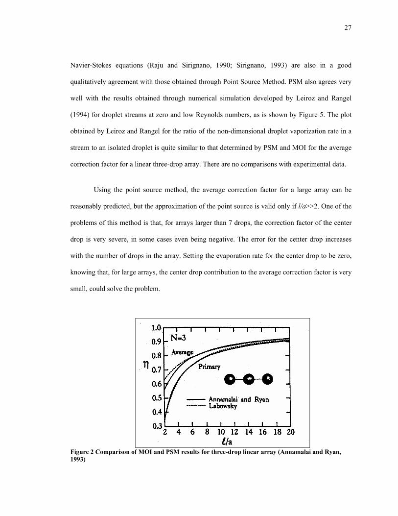
27

Navier-Stokes equations (Raju and Sirignano, 1990; Sirignano, 1993) are also in a good

qualitatively agreement with those obtained through Point Source Method. PSM also agrees very

well with the results obtained through numerical simulation developed by Leiroz and Rangel

(1994) for droplet streams at zero and low Reynolds numbers, as is shown by Figure 5. The plot

obtained by Leiroz and Rangel for the ratio of the non-dimensional droplet vaporization rate in a

stream to an isolated droplet is quite similar to that determined by PSM and MOI for the average

correction factor for a linear three-drop array. There are no comparisons with experimental data.

Using the point source method, the average correction factor for a large array can be

reasonably predicted, but the approximation of the point source is valid only if l/a>>2. One of the

problems of this method is that, for arrays larger than 7 drops, the correction factor of the center

drop is very severe, in some cases even being negative. The error for the center drop increases

with the number of drops in the array. Setting the evaporation rate for the center drop to be zero,

knowing that, for large arrays, the center drop contribution to the average correction factor is very

small, could solve the problem.

Figure 2 Comparison of MOI and PSM results for three-drop linear array (Annamalai and Ryan, 1993)

28

Figure 3 : Comparison of MOI and PSM results for a five-drop array (Annamalai and Ryan, 1993)

Figure 4: Comparison of MOI and PSM results for a seven-drop array (Annamalai and Ryan, 1993)

29

Figure 5: Ratio of the non-dimensional droplet vaporization rate in a stream to an isolated droplet – numerical solution (Leiroz and Rangel, 1994) 3.2. Extension of the PSM for Non-symmetric Arrays

As presented above the point source method was evaluated only for symmetric arrays and

only against other theoretical results. However, it has been demonstrated by Liu and Ruff (2001)

that while free-floating droplet arrays can be generated, the droplets are seldom of the same size

or spaced evenly. For non-symmetrical arrays, under the same assumptions, Eq. (7) can be used

to calculate a correction factor that can then be compared to experimental data. For two droplet

array, the correction factors for droplet 1 and 2, if droplet sizes are different, are given by:

( ) ( )1221

212111 aaalaaalal −−=η

( ) ( )2122

221122 aaalaaalal −−=η

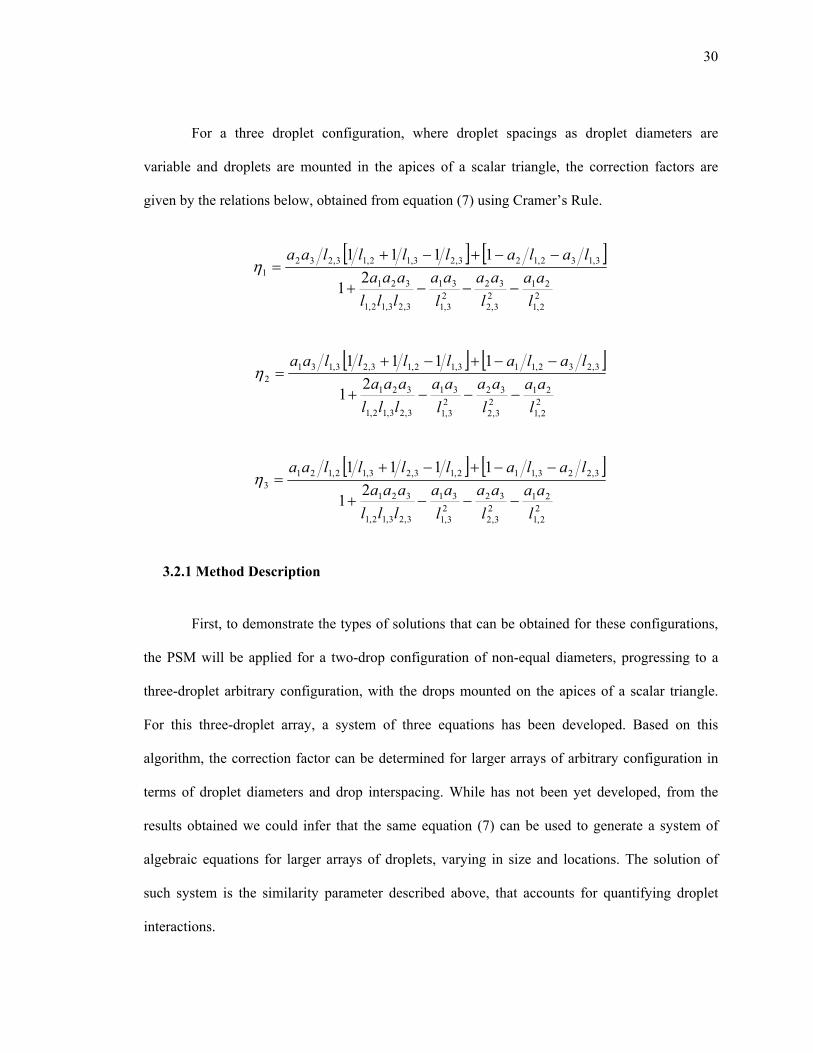
30

For a three droplet configuration, where droplet spacings as droplet diameters are

variable and droplets are mounted in the apices of a scalar triangle, the correction factors are

given by the relations below, obtained from equation (7) using Cramer’s Rule.

[ ] [ ]

22,1

212

3,2

3223,1

31

3,23,12,1

321

3,132,123,23,12,13,2321 2

1

1111

laa

laa

laa

lllaaa

lalallllaa

−−−+

−−+−+=η

[ ] [ ]

22,1

212

3,2

3223,1

31

3,23,12,1

321

3,232,113,12,13,23,1312 2

1

1111

laa

laa

laa

lllaaa

lalallllaa

−−−+

−−+−+=η

[ ] [ ]

22,1

212

3,2

3223,1

31

3,23,12,1

321

3,223,112,13,23,12,1213 2

1

1111

laa

laa

laa

lllaaa

lalallllaa

−−−+

−−+−+=η

3.2.1 Method Description

First, to demonstrate the types of solutions that can be obtained for these configurations,

the PSM will be applied for a two-drop configuration of non-equal diameters, progressing to a

three-droplet arbitrary configuration, with the drops mounted on the apices of a scalar triangle.

For this three-droplet array, a system of three equations has been developed. Based on this

algorithm, the correction factor can be determined for larger arrays of arbitrary configuration in

terms of droplet diameters and drop interspacing. While has not been yet developed, from the

results obtained we could infer that the same equation (7) can be used to generate a system of

algebraic equations for larger arrays of droplets, varying in size and locations. The solution of

such system is the similarity parameter described above, that accounts for quantifying droplet

interactions.

31

0

0.2

0.4

0.6

0.8

1

0 10 20 30 40 50

L/a

η

0

0.2

0.4

0.6

0.8

1

0 10 20 30 40 50

L/a

η PSM

0.8840.8750.822

isomm && /=ηDiameter (mm) Expt.

0.512 0.8600.476 0.7510.293 0.694

PSMPSM

0.8840.8840.8750.8750.8220.822

isomm && /=ηDiameter (mm) Expt.

0.512 0.8600.476 0.7510.293 0.694

isomm && /=ηDiameter (mm) Expt.

0.512 0.8600.476 0.7510.293 0.694

isomm && /=ηDiameter (mm)Diameter (mm) Expt.Expt.

0.5120.512 0.8600.8600.4760.476 0.7510.7510.2930.293 0.6940.694

Figure 6: Comparison between PSM and experimental data obtained in normal gravity, for a three droplet array performed by Liu. (2003); fuel: methanol, T=20C, p=1 atm.

Liu (2003) proved that experimental data obtained are in good qualitative agreement with

PSM and his findings are presented in Figure 6.

3.2.2 Results of the PSM for Non-symmetric Arrays

Calculations were performed for two-drop arrays of non-equal diameters and for three-

drop non-symmetrical arrays. The three-drop configuration consists of three drops of non-equal

diameter mounted in the apices of an equilateral triangle.

For a two-drop configuration, droplet 1 is larger than droplet 2 and the inter-drop spacing

cannot be less than the sum of the radii of the two drops (the drops do not collide and do not

coalesce). It has been observed that as the ratio of droplet radii increases, the smaller drop has

less of an affect on the larger drop and the correction factor of the larger drop is almost 1,

indicating that it behaves like an isolated droplet. However, the correction factor of the smaller

drop decreases dramatically to values significantly below unity, indicating that the evaporation

rate of the smaller drop will be considerably affected by the presence of the bigger drop. A

32

smaller drop that is in the wake of a larger drop will be affected even at large droplet inter-

spacing (l/a ~50). These results indicate that as the ratio of droplet radii increases, the droplet

interactions are present and strong even for large values of l/a, as shown in Figure 7.

When the droplets have comparable diameters, both are equally affected when they are

up to 15 or 20 radii apart. As the spacing increases, the droplet interactions are weaker and the

droplets behave like isolated drops. The diagram presented in Figure 7 illustrates this behavior.

Calculations were also performed for a three-drop configuration; the first drop is the

largest with the diameters decreasing for drops 2 and 3. As a condition of non-colliding and non-

coalescing, the spacing between drops cannot be less then the sum of the first 2 drops. Four

different three-droplet configurations were evaluated. In the first configuration, two droplets have

similar or nearly similar sizes and the third one has a much smaller diameter. As shown in Figure

8 and, the larger two drops behave like a two-drop array as we have seen in the previous analysis,

while the third, smaller drop is strongly affected by the other two. At closer distances between

droplets, the vaporization rate could be as small as 40% of the vaporization rate of an isolated

drop in similar conditions. The droplet interactions are predicted to be significant up to l/a~40.

The next three-droplet configuration we will consider is a single large drop with the other

two being considerably smaller but having similar diameters (). While the large drop behaves like

an isolated drop, the evaporation rate of the two smaller drops in the array decreases by up to

30% compared to an isolated drop. The behavior is similar to the previous case only for l/a>20.

When the droplets are closer than l/a=20, the effect on the smaller droplets is even stronger.

33

0

0.2

0.4

0.6

0.8

1

1.2

0 5 10 15 20 25 30 35 40 45 50

l/a

η

η1, a1/a2=1.5

η2, a1/a2=1.5

η1, a1/a2=5

η2, a1/a2=5

Figure 7 Calculated correction factor for a two-droplet array with different droplet sizes (a1/a2=1.5, a1/a2=5)

a1/a2=1.1, a1/a3=5

0

0.2

0.4

0.6

0.8

1

1.2

0 5 10 15 20 25 30 35 40 45 50

l/a

ηη1η2η3

Figure 8 Correction factor calculated for a three-droplet asymmetric array with two larger droplets of similar diameter sizes and a much smaller droplet in the wake of larger drops

34

a1/a2=1.3, a1/a3=7

0

0.2

0.4

0.6

0.8

1

1.2

0 5 10 15 20 25 30 35 40 45 50

l/a

ηη1η2η3

Figure 9 Correction factor calculated for a three-droplet asymmetric array with two larger droplets of near similar diameter sizes and a much smaller droplet in the wake of larger drops

a1/a2=3, a1/a3=5

0

0.2

0.4

0.6

0.8

1

1.2

0 5 10 15 20 25 30 35 40 45 50

l/a

η η1 η2η3

Figure 10 Correction factor calculated for a three-droplet asymmetric array with two smaller droplets in the wake of larger drop

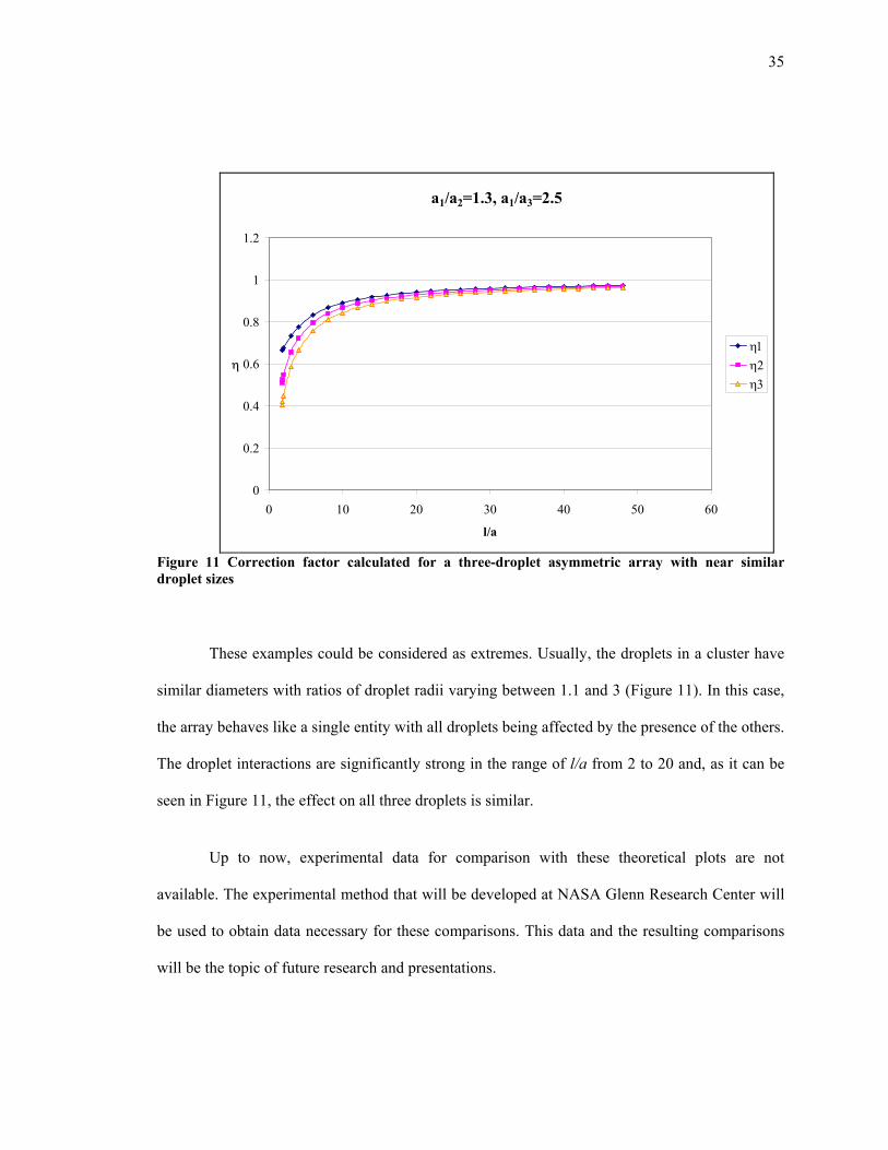
35

a1/a2=1.3, a1/a3=2.5

0

0.2

0.4

0.6

0.8

1

1.2

0 10 20 30 40 50 60

l/a

ηη1η2η3

Figure 11 Correction factor calculated for a three-droplet asymmetric array with near similar droplet sizes

These examples could be considered as extremes. Usually, the droplets in a cluster have

similar diameters with ratios of droplet radii varying between 1.1 and 3 (Figure 11). In this case,

the array behaves like a single entity with all droplets being affected by the presence of the others.

The droplet interactions are significantly strong in the range of l/a from 2 to 20 and, as it can be

seen in Figure 11, the effect on all three droplets is similar.

Up to now, experimental data for comparison with these theoretical plots are not

available. The experimental method that will be developed at NASA Glenn Research Center will

be used to obtain data necessary for these comparisons. This data and the resulting comparisons

will be the topic of future research and presentations.

36

While waiting for experimental investigation, a numerical model has been developed that

will be based on estimation of the same similarity parameter as in PSM and the data will be

validated against PSM and other theoretical and available experimental data from past

investigations present in the literature. Also, the numerical simulation results will be used to

support our future experimental investigation still in progress.

37

CHAPTER 4: FORMULATION OF THE NUMERICAL SIMULATION

In a real spray, the distance between droplets is small enough to allow droplets to

interact. One important conclusion inferred by several researchers was that for real sprays, a drop

is affected by its nearest neighboring droplets. Therefore, isolated drop studies are difficult to

extend to descriptions of complete spray systems. The most comprehensive theoretical models of

isolated drops are generally fairly complex methods and not amenable to the analysis of droplet

arrays or clusters. Some of them (Imaoka and Sirignano, 2004, 2005 and Yang and Wong, 2002,

for example) are expandable to and/or treat array of drops, under certain assumptions, but will

require prohibitively long computational times or do not predict individual burning rates but

rather an array burning or vaporization rate. As presented in the previous review, theoretical and

experimental studies have been performed that examined arrays of drops and streams and many

of the aspects of droplets evaporation and droplets interaction have been revealed. These

investigations have pointed the way towards new areas of research one of them being the

developed in the present research.

4.1 Overview

The effect of two- and three-dimensional configurations on these phenomena could be

important and should be quantified. However, three-dimensional interactive effects on heat and

mass transfer remain to be determined. Studies on these topics will undoubtedly start with arrays

having only a few drops. Nevertheless, the studies should be extended to arrays of a greater

number of drops for more direct application to practical sprays. As presented in recent studies,

methods developed up to now have several drawbacks, as indicated in Imaoka and Sirignano

(2005) whose model itself being still in progress and does not include thermal radiation effects.

Another difficulty is that the majority of them have not been compared with experimental data

38

taken in similar conditions as the model described by the theory. Through the review of this

literature and the development of an experimental method, it was found that many of the

theoretical or numerical studies are not sufficiently flexible to mimic an experiment as it would

have to be performed.

Therefore, a three dimensional model of symmetric and asymmetric arrays of fuel droplets

burning under microgravity conditions have been developed. The numerical simulation along

with the future proposed experiment described further in the project is a unique combination of

investigative methods that will provide support for future investigations and for understanding of

droplet interaction phenomena.

4.2 Assumptions, Justifications and Implications

4.2.1 General Assumptions

As previously stated, the model will mimic (as close as possible) the experimental

investigation, supporting in this way the experiments performed by Liu (2003) under normal

gravity and future experimental data obtained through a microgravity experiment in which the

formation of dilute and dense clusters can be created and stabilized before combustion is begun

allowing the spectrum of droplet interactions during combustion to be observed and quantified. In

this numerical simulation, each drop in the array will vaporize and burn according to the

conditions created by the environment around the droplet and also the array can be considered as

an entity. Therefore, the reaction will happen only if the temperature and fuel and oxidizer

concentrations are high enough to sustain the combustion. Furthermore, if all the fuel in a droplet

is consumed, it will be removed completely from the array. This approach is closer to what

happens in reality in the evaporation and combustion of groups of droplets. However, the fixed

position of the droplets during simulation will not allow quantifying the effect of droplet motion

39

due to the Stefan velocities. This assumption is valid as long as we refer to an array of droplets

surrounded by other arrays of droplets (as in the middle of a spray cloud) where the movement of

a droplet relative to other droplets is negligible. Also, this assumption will be valid on the time

constraints imposed during an experiment, i.e., the data are collected after the igniters are

removed and burning of the droplets is self-sustaining.

The model developed in this study accounts for radiative heat transfer using a Finite Volume

Method, Stefan convection, diffusion and finite-rate chemical kinetics, and unity Lewis number

but does not account for forced convection and for internal circulation within the droplet. The

assumptions made for the model are similar to those used in previous studies, i.e., a quiescent

environment, near zero Reynolds number, and gas-phase variable thermo-physical properties. The

temperature inside the droplet is considered to be uniform and constant throughout the droplet at

a frozen moment in time. The specific heat and thermal conductivity of the liquid fuel is assumed

to be variable in time according to gas-phase temperature near the droplet. The liquid-fuel

specific heat will be obtained using the curve fitting coefficients from tables (Perry’s Chemical

Engineers Handbook) (Table 1), with the curve approximated as function of temperatures ranging

from 293K to 337K (vaporization temperature) using Eqn. (8).

1000/)( 45

34

2321 TCTCTCTCCc p ++++= [J/mol-K] (8)

Table 1: Curve fitting coefficients for methanol (for temperatures in centigrade scale)

C1 C2 C3 C4 C5 Coefficients

1.0580E+05 -3.6223E+02 9.3790E-01 0 0

40

Similarly, the variation of thermal conductivity is simulated using two linear functions of

temperature, one ranging from 298K to 323K, having the limit values of 0.202W/m-K to

0.195W/m-K and the second from 323K to 348K, whose values at the margins are 0.195W/m-K,

respectively 0.189w/m-K. The values are from tables found in Handbook of Chemistry and

Physics. Only gas-phase phenomena are considered to drive the droplet combustion around the

droplet. The liquid-gas phenomena are included. Due to finite rate fast chemical reaction, the

oxidizer is consumed at the flame sheet and the flame sheet itself is very thin, being the limit

between fuel and oxidizer (McGrattan (2004)). There is no soot yield considered although the

simulation is able to account for soot production.

4.2.2 Water Absorption

The model does not consider water absorption of methanol droplets, investigating just pure

methanol droplet combustion in dry air. Water absorption is an important phenomenon that is still

under investigation, being proved that methanol droplets can and do absorb water during drop

burning lifetime. The burning rates would be retarded with water being absorbed and then

vaporized. However, the amount of water absorbed is not significant at initial stages of

combustion (Ross, 2001), and including thermal radiation effects, the gasification rates are lower

by about 10% (Marchese et al.) when water/methanol droplets are considered. The conclusion

inferred by Choi and Dryer (2001) in their comprehensive review (Ross, 2001) is that the water

diffusivity is not that important in the calculation of burning rates, one of the important output

parameters of the current work. Therefore, water absorption into methanol droplets during

combustion is neglected for the purpose of this study.

41

4.2.3 Effect of Reynolds number on Interacting Droplets: Near Zero Re Number

An important issue in the evaluation of droplet evaporation and interactions is that the

relative Reynolds number, e.g., the Reynolds number based on the local droplet conditions and

the relative velocity between the droplet and the ambient. Many researchers concluded that for

low relative Re numbers (0 to ~30), the droplet interactions are very strong, much stronger than

for higher Re (>50). The lower Re number regimes (0-30) are more relevant to practical sprays

flows, after the droplets have been decelerated from the spray injection conditions. In fact, if the

drop is moving with the surrounding flow, the Reynolds number could be assumed to go to zero.

Most of the studies were performed mainly for high and intermediate Re numbers limits for a

vaporizing droplet array or stream. The zero and low Reynolds number limit for a vaporizing

droplet stream is the logical next step beyond the classical isolated droplet theory resulting in the

d2-law. This issue has been investigated using direct numerical simulation and approximate

methods, but experimental studies for this case are not available yet. The investigation of

unsupported arrays of drops for zero relative Re number could offer a better understanding of the

droplets interaction phenomena. A combined theoretical and experimental approach for

unsupported arrays of drops for low Reynolds numbers would be a significant research

contribution that could provide relevant insight concerning droplet interactions and the

characteristics of droplet evaporation for arrays of fuel drops.

4.2.4 Internal Circulation within the Droplet

The presence of the internal liquid circulation due to droplet generation and deployment

techniques and heterogeneity of the surface temperature (Marchese and Dryer, 1996) has been

demonstrated and such internal circulation inside a pure fuel droplet enhances mass and heat

transfer inside the droplet. Evaluating the effect of this contribution is quite complex and would

42

require further computational efforts. Formulating and solving a comprehensive solution of the

complete problem is quite difficult for current computers to handle. Marchese et al. (1999),

approximated this effect using an “effective” liquid-phase conductivity (“enhanced mass and

thermal diffusivities” (Marchese et al., 1996), but this introduces a new parameter that must be

determined. In his solution, he found the droplet heat-up transient becomes slower, while the

burning rate or extinction phenomena are not greatly affected. Generally, good agreement with

experimental measurements is observed, even when the presence of internal circulation in the

liquid-phase is ignored.

4.3 Numerical Solution

Fire Dynamic Simulator computer code (FDS), publicly released by National Institute for

Standards and Technology, is a computational fluid dynamic numerical model of thermally-

driven fluid flow that solves Navier-Stokes equations for low-speed flow. It is easy to use and

adapt and has the main advantage of having the source files available for download from a public

website, unlike the majority of commercial computational fluid dynamics codes. Since its first

release in 2000, the code has been reviewed, improved and validated through numerous

experimental and theoretical investigations in the past years as presented in the Technical

Reference Guide (McGrattan et al., 2005), making it a valuable tool for fire research. Another

advantage of FDS is Smokeview, a software tool that works concerted with FDS and was

designed to visualize in two or three dimensions numerical simulations generated by FDS.

Therefore, taking into account all the advantages presented by FDS it was easier, less time

consuming and more reliable to use rather than writing a personalized code for this investigations

or using a commercial CFD code.

43

Initially, a modified version of Fire Dynamic Simulator computer code (McGrattan et al.

2005) – version 3.0 (FDS) was been used to simulate ignition and combustion of isolated droplets

and droplet arrays. The code was modified to account for thermal radiation for finite-rate reaction

using direct numerical simulation. The radiation subroutine contained in the code was originally

developed for a mixture-fraction combustion model but was adapted to calculate radiation heat

loss through boundaries using the finite rate combustion modeling based on CO2 and H2O

absorption coefficients under ideal, non-sooting gray gas assumption. The modifications were

made on version 3 of FDS and the radiation model was based on “RadCal” (McGrattan et al.

2005, Grosshandler, 1993). The modified radiation solver used a finite volume solution for the

thermal radiation equation using point-wise values of the mass fraction, temperatures and partial

pressures to determine the absorption coefficient throughout the computational domain. The finite

volume solver is used to determine also the radiation heat flux from the gas-phase back to the

vaporizing/burning droplet. To reduce the computational time involved, the radiation solver

skipped computation of variable specific heats for the species in the gas-phase. The assumption is

valid considering that there is not much of variation of temperature during self-sustained

combustion.

The initial data obtained using the modified version were in qualitative agreement with

other theoretical results for isolated drop combustion and with the combustion of droplet arrays as

presented in our previous work (Ciobanescu and Ruff, 2004) and these results will be also

presented later in this paper in Chapter 5. One difficulty encountered was a slight over-prediction

of the burning rates caused by over prediction of the temperatures. This behavior was

acknowledged by FDS authors and the code was further improved (McGrattan et al. 2005). The

fourth version of FDS offers the possibility of including radiation in calculations that involves

one-step chemical reaction. Also, the data obtained using the new version recently released

44

(2005) gave similar results with the modified version developed previously to model droplet

combustion. One other problem of the modified version was the large amount of CPU time

required to run a simulation. The new version (FDS_v4) offers improved CPU times for similar

cases, requiring 20% to 30% less CPU time than the modified version based on FDS_v3,

depending on grid resolution and complexity of the droplet configuration.

Considering all the above and the advantages of a “debugged” and improved code that

eliminated much of the errors of previous version used to create the modified version, we decided

to use FDS_v4 in the remainder of this investigation. FDS_v4 does include a finite volume solver

for finite-rate reactions that is used with either the gray gas or band model, similar to that

included in modified FDS. Another advantage of FDS_v4 is the possibility of varying the fuel

properties as a function of temperature, namely the specific heat and thermal conductivity of the

liquid fuel, giving the opportunity of more accurate predictions. However, because of the number

of simulations performed using FDS_v3 and the fact that the modified version 3 and FDS_v4

provided identical simulations, results obtained using the modified version of FDS_v3 will be

presented in the following sections.

4.3.1 General Equations

For the gas-phase, the equations used were the equation of state and the conservation

equations for total mass, momentum, and chemical species. The energy equation is not directly

solved, but its source terms are included in the equation for flow divergence. The partial

derivatives of conservation equations of mass, momentum and energy are approximated as finite

differences, and the solution is built on a three-dimensional, rectilinear grid and it has time as

fourth coordinate. The divergence constraint contains the influence of conduction, mass diffusion,

enthalpy diffusion, thermal radiation, and chemical heat release on the velocity divergence. A

45

Poisson equation for the hydrodynamic pressure was solved using a fast direct solver. Second

order temporal and spatial discretization schemes were used (McGrattan et al. 2005). Most of the

theoretical basis for the model is described in the Technical Reference Guide of FDS (version 4)

(McGrattan et al. 2005). Highlights of hydrodynamic, combustion and radiation model and also

details of the numerical method used by this research will be given below from the above cited

source:

Mass Conservation:

0=⋅∇+∂∂ uρρ

t (9)

Species Conservation:

( ) lllll mYDYYt

′′′+∇⋅∇=⋅∇+∂∂

&ρρρ u (10)

Momentum Conservation

( ) τρρ ⋅∇++=∇+

∇⋅+

∂∂ fguuu p

t (11)

Equation of Energy Conservation

( ) ∑ ∇⋅∇+∇⋅∇+⋅∇−=⋅∇+∂∂

llllr YDhTk

DtDphh

tρρρ qu (12)

The f term is the external force of the fluid. The term ptp

DtDp

∇⋅+∂∂

= u is a material derivative.

Equation of State

( ) MTMYTp il ℜ=ℜ= ∑ ρρ0 , (13)

where 0p is the background pressure.

This equation is valid only for low Mach number where the time step in the numerical

algorithm is influenced only by the flow speed, and the modified state equation leads to a

46

reduction in the number of dependent variables in the system of equations by one. The divergence

of the fluid flow u⋅∇ is given from the material derivative of the equation of state and

substituting the terms of energy and mass conservation equations. The specific heat of the

mixture is considered constant and is the summation of the product between temperature

dependent specific heats of the species and mass fraction of the species in the mixture. The

enthalpy is defined similarly.

The approximate form of divergence used in the calculations is:

dtdp

pTcqYDdTcTk

Tc plrlllp

p

0

0,

111

−+

′′′+⋅∇−∇⋅∇+∇⋅∇=⋅∇ ∑∫ ρρ

ρ&qu (14)

To account for the pressure rise in sealed enclosures, the pressure equation is given by the

integral of the divergence over the computational domain.

A simplified form of the momentum equation is also used in this formulation. Following

McGrattan et al. (2005), we start from Eqn. (11), substitute g∞+∇=∇ ρpp ~ , apply the vector

identity for second term in the right had side of momentum equation and decompose the pressure

term using Eqn. (14)

ppp ~11~~∇

−+

∇=

∇

∞∞ ρρρρ (15)

This results in a simplified form of Eqn. (11):

( )[ ]τρρρρρρ

ω ∇++−=∇

−+

++×−

∂∂

∞∞∞

fgu

uu 1~11~

2

2

ppt

(16)

The pressure equation is obtained by taking the divergence of Eqn. (16). The pressure term in the

pressure equation is decomposed and approximated (Eqn. 17) using the average density and the

values of the pressure from the previous time step.

47

ppp ~11~~1∇

−⋅∇+

∇⋅∇=∇∇

ρρρρ (17)

Whether the extra pressure term neglected or approximated (to simplify the numerical solution

for the pressure equation) is determined by its contribution to the creation of vorticity. In the

model investigated here, restoring baroclinic vorticity is automatically invoked and is described

in the FDS Technical Reference Manual (McGrattan et al. 2005).

The binary diffusion coefficient of a species diffusing into other species is given by:

Ω

×=

−

sm

M

TTD

Dlmlm

lm

2

221

23371066.2

σ (18)

where ( ) 1112 −+= mllm MMM , the Lennard-Jones coefficient is the average of the

corresponding species coefficients and DΩ is the diffusion collision integral. It is assumed that

nitrogen is the background species, therefore:

( )2,, NlDNSl DD ρρ = . (19)

4.3.2 Combustion Model

According to the FDS Technical Guide, the one-step reaction considers the general reaction of

oxygen and a hydrocarbon fuel approximated by Arrhenius equation, in our case, methanol,

where the reaction rate is given by:

[ ] [ ] [ ] RTEba eOOHCHBdt

OHCHd −−= 233 (20)

The values for B, a, b, and E have been taken from Stiech (2003) and Westbrook and Dryer

(1981) (Table 2.):

48

Table 2: Reaction rate parameters for methanol Property Value Units

B = Pre-exponential factor

(“BOF”)

3.12E12

smolcm

⋅

3

E = Activation energy 125,604

kmolkJ

a = exponent for oxygen

concentration (“XNO”)

0.25 -

b = exponent for fuel

concentration (“XNF”)

1.5 -

Table 3: Properties for fuel and products of combustion for methanol air reaction

Lennard-Jones

potential parameters

Species Diffusion

coefficient

s

m 2

Viscosity

⋅ smkg

Thermal

conductivity

⋅ KmW

Molecular

weight

mol

g

σ [Å] k

ε [K]

CH3OH 1.32 E-5 96.27E-7 0.01565 32 - -

O2 - - - 32 3.467 106.7

H2O - - - 18 2.641 809.1

CO2 - - - 44 3.941 195.2

The reaction between fuel and air takes place at a finite rate given by Arrhenius equation

(Eqn. 20) and the reaction zone is an infinitely thin sheet where the fuel-oxygen concentration is

high enough to sustain the combustion (McGrattan, 2005). Species properties as well as the

49

stoichiometric coefficients must be specified. In any cell where the reaction is “on” the chemical

reaction time is much shorter that any convective or diffusive transport time scale. Nitrogen is a

background species and does not participate in the reaction except as a diluent. The properties of

fuel and products of reaction are tabulated below (Table 3.) and are according to Perry’s

Chemical Engineers Handbook and JANNAF tables:

For methanol, the effective heat of combustion is 19,937kJ/kg, the heat of vaporization is

1100kJ/kg, and the thickness of the liquid is the droplet diameter. Although the thickness is very

small, the fuel will be considered thermally thick that allows the thermal conductivity of the

liquid to be specified (see the input files in the Appendix B). Also the ignition temperature is

specified, for methanol being the boiling point (64.7oC). The model does not consider the

convection within the liquid droplet.

4.3.3 Radiation Model in the Gas-phase

FDS solver uses the Radiative Transport Equation for an absorbing, emitting and

scattering medium. A summary of the general model used by FDS and pertinent to our

investigation will be described below. This model is included in the FDS_v4 Technical Reference

Guide (McGrattan et al., 2005). The radiative transport equation used in FDS is

( ) ( ) ( )[ ] ( ) ( ) ( ) ( ) ( )∫ Ω′′′Φ+++−=∇⋅π

λλ πλσλλσλκ

4

,,4

,,,,,, dIBII ss sxssxxsxxxsxs (21)

where “ ( )sx,λI ” is the radiation intensity at wavelength λ, “s” is the direction of the intensity

vector, ( )λκ ,x and ( )λσ ,x are the local absorption and scattering coefficients, and B(x, λ) is

the emission source term.

50

FDS can operate in two modes when solving the RTE, specifically a gray gas model and

a wide-band model. Due to the lack of soot in the gas-phase, the lumped gray gas assumption

may produce significant over-predictions of the emitted radiation (McGrattan et al., 2005).

The wide-band model implies that for each band, the RTE can be derived and the source

term can be written as a fraction of the blackbody radiation. The total intensity is the summation

of all the intensities integrated over each band, and determined using the mean absorption

coefficient inside the band. The radiative heat loss term is the divergence of the radiation flux in

the gas. The gray gas model assumes that the spectral dependence is lumped into one absorption

coefficient and the source term is given by the blackbody radiation.

To select the right model to use in this application, the wide-band model has been tested,

using six spectral bands (CH4 as fuel) versus the gray gas model, for single droplet combustion.

The source term in the RTE is based only on the gas (CO2 and H2O mixture) temperature and

composition. Upon analysis, it was concluded that the slight increase in mass burning rates and

temperatures using wide-band model (less than 7% for mass burning rates and less than 3% in

temperatures) does not overcome the dramatic increase in the computational time. Therefore, for

the purpose of this research, the gray gas model for radiation solver has been chosen.

The RTE is solved using a finite volume solution similar to that used by Raithby and

Chiu (1990) and is based on “RadCal” developed by Grosshandler (1993).More details about the

model can be found on Technical Reference Guide (McGrattan et al., 2005). To increase the

accuracy of the radiation model, the number of solid angles may be increased and the time and

angle increments could be reduced. However, this technique will considerably increase the

computational time.

The modified version of FDS_v3 used the gray gas approximation of the mixture-fraction

model. The modifications consisted of creating a subroutine that will invoke the radiation solver

51

even if the absorption coefficient is not specified (the mixture-fraction combustion model) and if

the finite-rate reaction is present. The radiation solver would compute the mean absorption

coefficient based on gas temperature using one band. Considering that the size of the droplet is

relatively small and the radiative heat loss is lower than convective heat loss, it was assumed that

the over-prediction of the emitted radiation will not greatly affect the overall heat release.

Alternate methods of solving the RTE using FDS_v3 would also significantly increase the

computational time. Therefore, this approach seemed to be the reasonable choice. FDS_v4,

however, offers a more accurate modeling of gas-phase radiation at reasonable computational

times and has been used in many of the simulations. The data for radiative heat loss obtained

from the modified FDS version and FDS_v4 were compared and the results are in qualitative

agreement. The main improvement was in the computational efficiency of the code as well as in

code stability. Simulations of more complex cases were made possible using FDS_v4.

4.3.4 Numerical Algorithm

The numerical method will be very briefly described here; it is fully described in the

FDS_v4 Technical Reference Guide (McGrattan et al., 2005). For all scenarios, all spatial

derivatives are approximated by second order finite differences on rectilinear grid and the flow is

updated with a second order predictor-corrector time step. The scalar quantities are approximated

at the center of the cell and all vector quantities are defined at center of the cells faces, normal to

the face. For a DNS simulation, the diffusion coefficients, dynamic viscosity, and thermal

conductivity are defined at the center of the cells. For the time discretization, the pressure, density

and mass fractions are estimated using an Euler step from the initial condition quantities,

considered known. The divergence is calculated from these quantities and then the Poisson

equation is solved with a direct solver. The corrector step will adjust the thermodynamic

quantities at the next time step. The pressure is computed from estimated quantities and after that

52

the velocity vector is corrected. The mass and energy equation are combined using the divergence

of the flow field which is discretized on both predictor and corrector steps. The convective terms

are written as upwind-biased differences in the predictor step and downwind biased differences in

the corrector step (McGrattan et al., 2005), while the material and thermal diffusion terms are

central differences (same for corrector and predictor steps) and the temperature is calculated from

equation of state using the density.

For finite-rate reactions, the heat release is averaged over a time step for a given cell (ijk),

using the density of the gas in a cell, the mass fraction of the fuel and the heat of combustion

(specified in the input file). Because the specifics of the one-step reaction, the chemical time of

the reaction is much shorter than the time step of the solver. Therefore, all the processes will be

considered “frozen” at the beginning of the time step. The mass fractions of the species are

updated before the convection and diffusion update. The mass fractions of the fuel and oxygen

are calculated using a Runge-Kutta second order method, for each grid cell using the reaction rate

parameters as given data. The RTE is integrated over discrete solid angles and over the rectilinear

grid (Howell and Siegel, 2002). The detailed scheme is presented in reference (McGrattan et al.,

2005) and it has no particularity for the finite-rate reaction.

A peculiarity of the DNS calculations for one-step chemical reaction is the evaluation of

the convective flux to the wall (a wall being any “solid” surface defined as either boundaries of

the computational domain or user-defined obstructions, in our case the droplet surface).

For the thermally thick wall (or solid), a one dimensional heat transfer calculation is

performed at each boundary cell of the solid (the droplet, in the current study). The solid is

partitioned in a number of cells. The temperatures are updated using a Crank-Nicholson scheme

and the boundary condition

53

( )44 TdqqxTk rc εσ−′′+′′=

∂∂

− && (22)

is discretized, the radiative term being linearized.

The technical guide has further detailed descriptions of the discretization of momentum

and pressure equations. Of importance is to notice that due to very small time steps involved in

the simulations performed and fine grids used, the main constraint for the time step is the von

Neumann criterion. The pressure equation is obtained from the divergence of the momentum

equation as a Poisson equation which is solved directly.

4.3.5 Problem Geometry

The general configuration that will be solved using the numerical method presented in the

previous sections consists of a computational domain spatially discretized using rectilinear grid.

Generally, a coarse grid was used for the entire computational domain and a finer grid embedded

into the coarse grid was used around the droplet cluster. The coarser grid has its cell dimension

equal to the biggest droplet radius in the array and the finer grid has the cell dimension equal to

the smallest droplet radius in the array. The droplet cluster is positioned at the center of the

computational domain. Droplets are represented by cubic obstructions created using four or more

cells. A special feature of the code allows defining the edged as curves by “cutting” the sharp

corners and avoiding the creation of steep temperature gradients at cube corners. When visualized

using Smokeview, the droplets have a quasi-spherical shape. The geometric configuration of each

case studied will be presented in the Chapter 5 that will follow.

Each cluster is ignited using four igniters, equally positioned respective to the center of

the cluster. The igniters are defined as parallelepipeds and have the cell walls facing the droplets

54

heated to a specified temperature (3000ºC). The igniters are at 20ºC at the initial time (t=0) and

the temperature is increased using a defined linear function of temperature versus time for the

0.25s, time when the temperature reaches the maximum. The maximum temperature is

maintained for another 2.25s. After 2.5s from the initial time the igniters are removed from the

computational domain.

There is no temperature gradient normal to the surfaces, the solid is considered thermally

thick and the boundary layer is solved using DNS. Gas phase temperatures are defined at cell

centers, while the velocities and other vector parameters are defined at the cell face’ centers.

The planes that form the boundary walls of the computational domain are considered

open, denoting a passive opening to the outside.

4.4 Burning Rate Calculation

Although the mass burning rate is one of the FDS outputs, the results produced are just a

verification of the total heat release to the boundaries and should be carefully evaluated. To

estimate the droplet mass burning rate, a separate algorithm was developed, based on the

temperature, velocity, species mass fractions and density for each node in a plane of the

computational domain. In Figure 12 below, four of the six planes used to estimate mass burning

rates are shown. Each plane represents a slice through computational domain at a specified

coordinate (xmin., xmax., ymin, ymax zmin, or zmax). This slice is divided into rectangular cells

(following the user specified spatial grid) and, at each node, the specified combustion parameters

values are calculated stored by the code into an ASCII slice file. The file provides values for the

entire slice but the data used to determine the burning rate are only those that are inside the faces

of the cube defined by the intersection of the defined planes. For example, for a slice defined at

55

xmin, the face of the cube will be defined by the intersection of the slice with x-ymax, x-ymin, z-ymin

and respectively z-ymax planes.

Figure 12: Slice planes around the droplet

Given this geometry and knowing all computational parameters on the six faces of the

volume surrounding the droplet, the burning rate is obtain by numerical integration of Eqn (23)

( ) dAm ijij uρ=& (23)

over all six planes surrounding a droplet. Data used to calculate the burning rate are collected

after the igniters are removed and the mass fraction of the fuel, temperature, Stefan flow

velocities and density for each node are averaged for a time increment and for each drop in a

cluster. The slice position has been carefully chosen to be inside the flame front to account for the

parameters of the investigated evaporating droplet Figure 13.

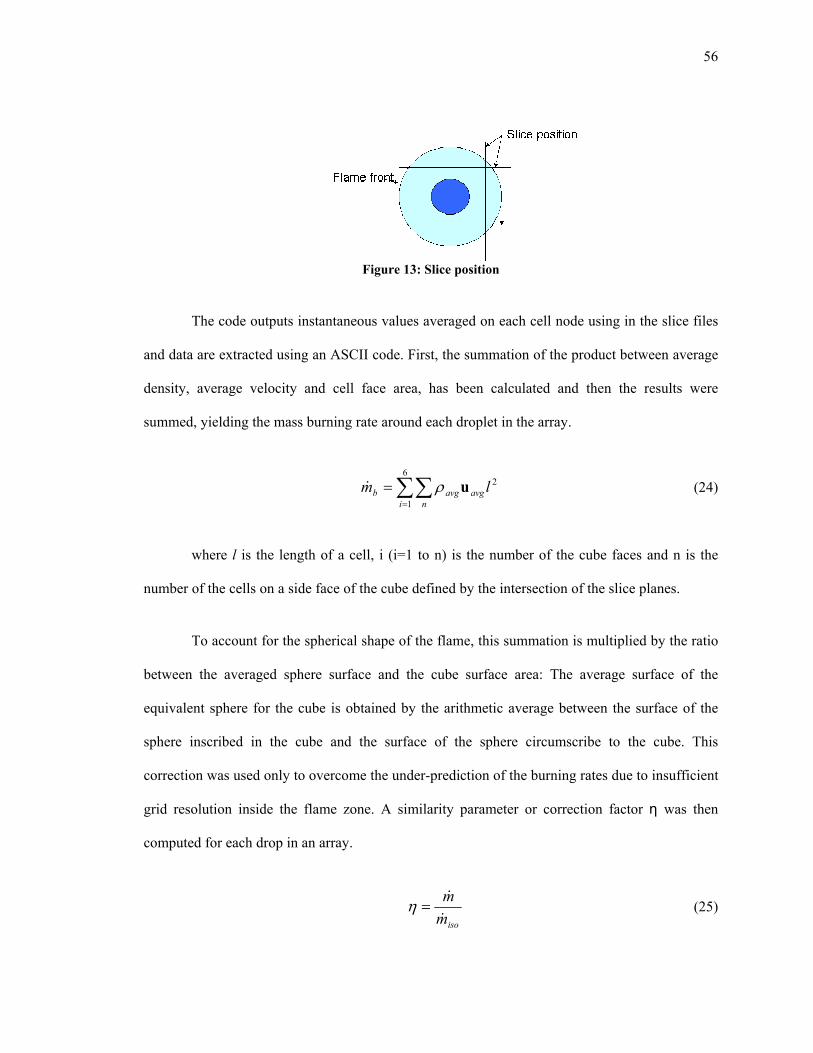
56

Figure 13: Slice position

The code outputs instantaneous values averaged on each cell node using in the slice files

and data are extracted using an ASCII code. First, the summation of the product between average

density, average velocity and cell face area, has been calculated and then the results were

summed, yielding the mass burning rate around each droplet in the array.

∑∑=

=6

1

2

i navgavgb lm uρ& (24)

where l is the length of a cell, i (i=1 to n) is the number of the cube faces and n is the

number of the cells on a side face of the cube defined by the intersection of the slice planes.

To account for the spherical shape of the flame, this summation is multiplied by the ratio

between the averaged sphere surface and the cube surface area: The average surface of the

equivalent sphere for the cube is obtained by the arithmetic average between the surface of the

sphere inscribed in the cube and the surface of the sphere circumscribe to the cube. This

correction was used only to overcome the under-prediction of the burning rates due to insufficient

grid resolution inside the flame zone. A similarity parameter or correction factor η was then

computed for each drop in an array.

isomm&

&=η (25)

57

The correction factors were calculated imposing the no collision or coalescence condition

generated for each configuration. Figure 14 shows an example of the format of the slices in the

computational domain, obtained using Smokeview_v4.0, a visualization code provided by NIST

team along with FDS.

Figure 14: Visualization of the slice positions in a computational domain for two droplet array

For multiple droplets configurations, several slices will be defined in the input files for

FDS, around each droplet being defined four slices providing necessary data.

4.5 Ignition Characteristics

For the finite-rate model, the heat loss controls the combustion phenomena. The

minimum ignition energy was analytically calculated using models presented by Kuo (1986) and

Turns (2000) as being the energy necessary to raise the temperature of a spherical volume of air-

fuel mixture to the stoichiometric flame temperature.

58

3,min 6 qstoichairairp dTcE πρ ∆= (26)

( )

5.0

1ln

+Φ

=B

dair

fq ρ

ρ (27)

Where dq is the air-fuel mixture diameter, Φ is the equivalent ratio and B is the Spalding transfer

number. Following this model, the following Minimum Ignition Energy (MIE) values have been

found for methanol.

Table 4 Minimum ignition energy for various pure methanol droplet diameters Drop diameter

[mm]

0.3 0.5 1.0 2.0

MIE [J] 0.41 1.91 15.3 122

In our model, the ignition is performed by an external source and heat is supplied to the

environment around the droplet. The external source is defined as four parallelepiped

obstructions, whose walls are hot in the proximity of the droplets (the walls facing the droplets).

Their size is similar to the size of the droplet. It was observed that the reaction begins to occur

after at least 0.4s when four igniters having 3000ºC wall temperature are applied. These findings

are in concordance with the experimental and numerical data obtained by Marchese and Dryer

(1999) where they observed the beginning of the reaction after 0.45s during their computational

investigation for an n-heptane 1.325mm droplet and surrounding air temperature of 1208K. Also,

based on previous experiments performed by several researchers (Faeth and Olson, 1968, Dryer

and Marchese, 1999), for methanol droplets the ignition time (the time required to get to flame

59

temperature) varies from 0.5s to 1.5s, depending on droplet diameter and surrounding

temperature.

To determine the ignition time, several cases were simulated, varying the number of

igniters from one to four, igniters’ wall temperature in the range of 500ºC to 6000ºC and the

ignition time from 0.5s to 2.5s.

For the heat release to be high enough to sustain the combustion reaction, it was

determined that four igniters were necessary and that they had to be energized for at least 1.5s.

Due to steep temperature gradients created during the sudden ignition, a ramp function of time

has been applied for the first 0.25s and the total ignition time was increased to 2.5s. During this

time, the temperature will linearly increase from 20ºC to 3000ºC.

A sensitivity study was performed to determine if the igniter temperature impacted the

burning rate of the droplets. Igniter temperatures between 3000ºC and 6000ºC were evaluated

and no influence on the combustion parameters during or after ignition was observed.

For multiple droplet combustion, a shorter ignition time was applied (2.0s) due to the

increased mass flux into the reaction zone.

4.6 Limitations of the Model and Error Margins

According to FDS_v4 Technical Reference Guide (McGrattan et al., 2005), the general

limitations applicable to our model are related to the rectilinear geometry, fire growth and spread,

combustion model and radiation. The FDS_v4 code is limited to all cases involving low speed

flow, ruling out any scenario that involves flow speeds approaching speed of sound.

The only limitation of our model due to the use of the rectilinear grid is in some

situations where certain geometric configurations do not conform to the rectangular grid. To

60

offset the effect of sharp edges, there is a technique in FDS_v4 to lessen the effect of “saw-tooth”

obstructions used to represent nonrectangular objects, and it was used to reduce steep temperature

gradients at the corners of the cubes representing the droplets. Caution has to be involved when

using the “saw-tooth” feature because the volume is reduced by this approximation of the curved

boundaries, mostly on a coarse grid, and the corresponding (by volume) droplet diameter could be

significantly smaller.

While the code allows using multiple meshes that “leak” one onto the other, meaning that

the coarser mesh will uses the data from the finer grid at its boundaries, when a finer grid

embedded into a coarser grid, both grids may behave independently and no data will “leak” into

the coarser grid. In some cases the overlapping of the grids may cause unsteadiness, leading to a

disruptive burning phenomenon. This can be overcome by using the grid meshes that share a

boundary instead of overlap.

For models where the heat release rate is predicted, the uncertainty of the model is

generally higher, the reasons for this being that the physical processes of combustion, radiation

and solid phase heat transfer are more complicated than their mathematical representations in

FDS and that the results of calculations are sensitive to both the numerical and physical

parameters (McGrattan, 2005). However, local velocities calculated using FDS_v4 are in the

range of 5% to 20% of experimental measurements and do not introduce significant deviations in

the predicted quantities greater than experimental investigations.

The combustion model involves the finite-rate assumption and this global approach for

combustion is still an area of research. Generally, most of numerical and analytical approaches

used both mixture fraction or finite-rate reaction but both of them were based on one step

chemical kinetics, their analyses producing reliable results while predicting combustion

61

parameters. However, if the level oxygen concentration at infinity is below 10%, the mixture

might not burn unless certain modifications are made to the input files.

Radiative heat transfer is included in the model via the solution of the radiation transport

equation for a non-scattering gray gas. The equation is solved using a technique similar to finite

volume methods for convective transport. One of the sources of error is the radiative heat flux

from the fire to the fuel surface. The error is due to a combination of insufficient grid resolution

in the boundary layer, and uncertainty in the absorption coefficient and flame temperature

calculated by the numerical code. As a result, the heat flux to the fuel surface is often over-

predicted (as per validation results presented in Technical Reference Guide, McGrattan et al.

(2005)). The radiative flux in the near-field, where coverage by the default number of angles is

much better, is better predicted.

The accuracy in calculation of flow velocities is very good, knowing that a corrector

predictor scheme is used to solve the divergence. The errors in calculating the normal velocities at

one cell face are several orders of magnitude less than the characteristic flow velocity. Using a

direct fast solver of the Poisson (pressure) equation had led to relative errors between the

computed and the exact solution of the discretized Poisson equation smaller than 10-12

(McGrattan, 2005).

One of the most important errors is related to the discretization of governing equations.

FDS_v4 uses a second-order accurate spatial and temporal numerical schemes, meaning that the

discretization is directly affected by the grid resolution. Halving the grid for example will reduce

the discretization error by a factor of 4, but that does not have to have a similar reflect for the

output results. Sensitivity tests have to be performed to quantify the errors on the output

quantities (sensitivity analysis and validation will be presented in the following chapters).

62

CHAPTER 5: RESULTS OF THE DIRECT NUMERICAL SIMULATION

5.1 Overview

Several factors have been studied before starting to investigate the combustion of

multiple droplets. For example, the sensitivity of the temperature and burning rates to domain size

and grid size (number of cells into a domain and cell size), ignition time, temperature of the

igniters and number of igniters used must be determined. As it has been shown in previous

sections, a large diversity of experimental, numerical and analytical studies of isolated droplets

have been developed in the past decades, providing data with which to compare the numerical

simulations of single droplet combustion.

The assumptions made in the beginning of Chapter IV are valid for all the cases studied

and presented in the next sections. The droplets combustion occurs in a quasi-quiescent

environment, considering unity Lewis number, Stefan convection, diffusion, gas-phase variable

thermo-physical properties, radiative heat transfer, and finite-rate chemical kinetics. There is not

considered water absorption by the methanol droplets, nor internal circulation or forced

convection considered.

The droplets are considered fixed in space and they do not move due to Stefan velocities.

However, the velocities due to thermal convection are considered when calculating burning rates.

The Reynolds number for all the investigated cases is considered to be near zero. If for single

droplet combustion, as shown in the next subchapter, the Reynolds number varies from 0.2 to 0.5,

following similar calculations, for two and three droplet arrays, the Reynolds number varies from

0.3 to 0.05.

63

To investigate grid and domain sensitivity as well as to validate the code against

theoretical and experimental results provided by studies found in literature, we developed single

droplet simulations that will be presented in the following sections. Therefore, the next step was

to investigate multiple droplets arrays, starting with two-droplet arrays and continuing with three-

droplet arrays.

5.2 Isolated Droplet Combustion

General assumptions stated previously in the above sections apply to all of the isolated

droplet combustion cases studied. In addition to that, the assumption of near zero Reynolds

number was based on average Re number calculated using average density and velocity values at

L=1mm distance from the droplet. The viscosity value used is from Table 3.

µρuL

=Re (28)

where the average density is in the range of

−= 328.025.0mkgρ , the average velocity is in

the range of

−=

smu 017.00083.0 , and viscosity

⋅−=

smkgE 0727.96µ .

The average Reynolds number obtained varies from 0.23 to 0.45 as function of droplet

diameter (droplet diameter varies from 2mm to 1mm). Therefore, the assumption of near zero

Reynolds number holds.

64

5.2.1 Grid Characteristics and Sensitivity Simulations

The grid characteristic dimension or the optimal grid size was initially established by

estimating the characteristic flame diameter using

52

=

∞∞

∗

gTcQD

pρ

& (29)

This first estimation is stating value. The time step is very important in establishing the

grid size. Therefore, the estimated value of the cell size will be adjusted using the time step

increment. This adjustment is made iteratively, by running several cases, using the as initial case

the estimated value given by Eq. 29. For the next cases, the grid will be gradually increased as

number of cells. A factor that has to be monitored is the time step size from the output data file. If

the time step starts to decrease dramatically, the cell size has to be increased for the next case.

The size of the time step is normally set automatically by dividing the size of a grid cell

by the characteristic velocity of the flow (McGrattan et al., 2005). During the calculation, the

time step is adjusted so that the CFL condition is satisfied. The default value of the time step is

( ) gHzyx 31

5 δδδ where δx, δy, and δz are the dimensions of the smallest grid cell, H is the

height of the computational domain, and g is the acceleration of gravity. Another condition that

has to be satisfied when using small fine grids (cell less than 5mm) is

1111,,max2 222 <

++

zyxt

ckD

p δδδδ

ρυ , (von Neumann criterion) (30)

65

where viscosity, material diffusivity and thermal conductivity were used. If the velocities

developed during combustion are too high compared to grid cell dimension, the time steps

become very small, causing the code to enter an infinite loop.

Another parameter considered was the concentration of methanol vapor around the

droplet. The fuel concentration has to be high enough for the reaction to take place. However,

since the mass fraction of fuel is averaged over a cell, the value will generally be under-predicted

and, if the grid is too coarse, ignition times will have to be extremely long or no ignition will

occur. The use of finer grids can solve this problem and it was found that a cell dimension of one

half of the smallest droplet diameter used in the array or smaller is sufficient for a droplet to burn.

Due to the complex nature of the factors that had to be considered, including the total CPU time

for each case (reducing cells size by half will incurs a 16-fold increase in total CPU time); each

case had to be evaluated to determine the optimal grid. There was no general grid dimension set

for all cases.

Grid sensitivity tests (Table 5) have been performed in addition to those already

performed by the authors of FDS and described in the technical guide. To study grid sensitivity

for the current investigation, several cases were created using different grid sizes for a single 2

mm droplet. Droplets were ignited using four igniters, at 3000ºC. Igniters were removed after

2.5s for the cases studied.

The maximum temperature is averaged in a cell and because the flame sheet is very thin,

and the temperature is averaged at the center of each cell, the adiabatic flame temperature will not

be achieved (Note: for methanol, the adiabatic flame temperature is 1904 oC). It was observed

that using smaller domains, for a 4 mm droplet FDS_v3 and the modified version of FDS_v3

over-predicted the flame temperatures. As we reduce the cell size the temperatures will slightly

66

increase for FDS_v4. A smaller domain was used for sensitivity analysis under the same

conditions as the previous analysis and the same conclusions were reached. The maximum

temperature will increase by about 20% when the number of the cells in the grid increases by 23

but with a dramatic cost in computational time (almost 10 to 15 times longer). Also the radiation

subroutine increases the CPU time by about 25%. The data were collected at 1.5s after the

igniters were removed from the computational domain and averaged for a sampling time of

0.002s. Mass burning rates were slightly affected by the grid size, increasing the grid size by a

factor of 2 for each axis caused in increase in the burning rate of about 8.5%. The calculated mass

burning rates were 2% to 14% higher than the bulk mass burning rate predicted by the code using

the total heat rate due to combustion.

Table 5: Grid sensitivity analysis as a function of temperature for a 2 mm droplet burning in air and a domain size of 64mm/side

Max. Temperature [oC] Case Number of cells

FDS_v3

modified

FDS_v4

no Rad.

FDS_v4

Rad.

Case 1 64x64x64 1210 1051.8 1008

Case 2 80x80x80 1140 1108 1096

Case 3 96x96x96 1190 1220 1153

The mass burning rates are governed by the Arrhenius equation and therefore affected by

the variations of the temperature due to the asymptotic relation between mass burning rates and

temperature. Considering this aspect, the computational domain size has to be large enough to not

influence the temperature. As the domain increases in size, the combustion parameters become

67

independent of the domain size as shown in Table 6 below. For single droplet, burning rates

become domain size independent for dimensions larger than 40 mm x 40 mm x 40mm (403 mm).

Table 6 Domain size dependence for a 2mm droplet burning in air, using a grid cell size of 1mm

Case Domain size

[mm]

Max. Temperature

[oC]

Burning rate

[1.0E-07*kg/s]

Case 4 203 1155.5 2.475

Case 5 303 1084 2.678

Case 6 403 1010.2 2.753

Case 1 643 1008 2.757

Temperature Distribution after 4.0s of Simulation (Case 4)

0

200

400

600

800

1000

1200

1400

0.E+00 2.E-03 4.E-03 6.E-03 8.E-03 1.E-02 1.E-02 1.E-02 2.E-02 2.E-02 2.E-02

x [m]

T [ºC]

Figure 15 Temperature distribution for a 203mm computational domain for a single droplet burning in atmospheric pressure (case 4), positioned at the center of the domain.

68

Temperature Distribution after 4.0s of Simulation (Case 6)

0

200

400

600

800

1000

1200

0.E+00 5.E-03 1.E-02 2.E-02 2.E-02 3.E-02 3.E-02 4.E-02 4.E-02

x [m]

T [ºC]

Figure 16 Temperature diagram for a 403mm computational domain for a single droplet burning in atmospheric pressure (case 6), positioned at the center of the domain

Another analysis performed concerned the variation of the temperature and burning rates

with grid size (cell size). Cases were investigated employed cells of 1mm and 0.5mm, for various

domain sizes.

Doubling the number of cells of the grid for each axis (the number of cells increase by a

factor of 8), for same domain size, the burning rates increase by less than 8%. The mass burning

rates increase by about 11% as the domain size is increased from 203mm to 403mm for grid cell

size of 1mm and 5.5% for a cell size of 0.5mm. For the finer grids, the burning rates are not as

sensitive to the domain size.

69

Table 7 Grid sensitivity analysis for a 2mm droplet burning in air

Case Domain size

[mm]

Number of cells /

cell size [mm]

Max. Temperature

[oC]

Burning rate

[1.0E-07*kg/s]

Case 4 203 203

1mm

1155.5 2.475

Case 9 203 403

0.5mm

1197.8 2.67

Case 5 303 303

1mm

1084 2.678

Case 12 303 603

0.5mm

1074.5 2.704

Case 6 403 403

1mm

1010.2 2.753

Case 13 403 803

0.5mm

1016.5 2.815

Increasing the number of radiation angles from 100 to 200 and also decreasing the angle

increment from 5 to 3 time steps does increase the maximum calculated temperature by 9% to

10% due to a more accurate calculation of radiation loss (decreasing the heat loss due to

radiation) but there was less than a 5% increase on predicted mass burning rates compared with

the 203 grid size case). However, the computational costs are dramatic (the CPU time doubled

compared to using the wide band model).

Nevertheless, a combination of fine grid resolution and a fine tuning of the RTE solver

will provide a more realistic simulation. Due to the extensively long computational time, this type

of case will not be investigated at this time, but the results from previous tests provided us with

enough elements to conclude that this solution is possible.

70

The calculated burning rates are in excellent qualitative agreement with the d2-law and

the values obtained are in excellent agreement with analytical solutions obtained by direct

calculation using theoretical droplet combustion model presented in Turns (2000). The mass

burning rate calculated using the ideal droplet combustion yielded a value of 3.83E-07 kg/s for a

2 mm droplet diameter and the calculations are presented in Appendix A. However, studies

performed by Faeth and Olson (1968), Marchese et al. (1996, 1999), Dryer et al. (1996), Dietrich

et al. (1995, 1997, 1999) concluded that the experimental values of mass burning rates to be

smaller that the values calculated using d2-law.

The burning rates were found to be affected by the grid size, and less affected by the

domain size (slightly more affected for small computational domains); therefore a grid size that

satisfies the ignition condition, i.e., cell size to be at least half of the smallest droplet in the array,

will be used for the simulation of clusters of droplets. Combustion parameters for two and three

droplet arrays become domain independent for a domain size larger than 403mm. If the distance

between droplets increases, the domain size has to be increased accordingly.

5.2.2 Validation Tests

For validation purposes, several test cases were created to investigate droplet combustion

using a single droplet. Comparisons for multiple droplets and arrays will be presented in

following sections) For this case, the droplet diameter was defined as a 2 mm solid cube filled

with liquid methanol that vaporizes with smooth edges to simulate a spherical droplet and reduce

steep gradients at the droplet surface. The grid size is specified to be 64x64x64 (1mm cell

characteristic dimension). Ignition occurs by four igniters that rapidly ramp up to 3000K at the

start of the simulation. The igniters are removed from the domain after 2.5 sec. All data are

collected 1.5s after igniters are removed and the duration of simulation varies from 1.5s to 20s.

71

Burning rates and temperature variations have been evaluated through these simulations. The

oxygen concentration has been varied from 10% O2 by volume to 75% O2 by volume and the

results are presented in Table 8.

Burning rates constants K were estimated using the d2-law and the ideal combustion

model for an isolated droplet (Turns, 2000).

sl

f

r

mK

ρπ2

&= (31)

where, lρ is methanol density, sr is droplet initial radius and fm& is the mass burning rate.

Table 8 Validation analysis for a 2.2 mm burning droplet in air at 10%, 15%, 21%, 35%, 50% and 75% oxygen

Case: Oxygen

Concentration

Max.

Temperature

[oC]

Burning rate

[kg/s]

Equivalent

K [mm2/s]

K [mm2/s]

Marchese et

al. (1999)

Case 15 10% 375 no burning - -

Case 16 15% 1060 2.73E-07 3.56E-01 0.4E-01 18% O2

Case 17 21% 1010.6 3.29E-07 4.29E-01 0.35 – 0.48

Case 18 35% 1070 3.54E-07 4.62E-01 6.0E-01 30% O2

Case 19 50% 1126.5 4.07E-07 5.31E-01 -

Case 20 75% 1121.8 3.83E-07 5.00E-01 -

The low mass burning rate value obtained for the 75%O2 case is caused by the flame

being too close to the droplet. The slice is “cutting” through the flame and the instantaneous

densities and velocities are not adequately resolved using this grid resolution (cell size is 1 mm).

72

For a more accurate prediction of the burning rate, a finer grid would be needed for this particular

case, although the error is less than 10% of the equivalent ideal burning rate calculated using d2-

law, and may be considered acceptable. However, the data from this particular simulation are

excluded form the final analysis.

The graph from Figure 17 was obtained by using the same slope-intercept 1.0 as in Figure

18 and estimated burning rates constants K as slopes. The burning rate constant K was estimated

using Eqn. (28), considering ideal combustion. The K values are less than 10% lower than those

obtained by Marchese and Dryer (1999) through numerical and experimental predictions, which

is a very good quantitative agreement (within the quoted experimental uncertainty). The lower

values for K could be also attributed to slight over-prediction of thermal radiation by FDS_v4

code and also by the fact that their predicted K values are obtained over the first 1.5s of burning

history, while the estimated K values tabulated above from are obtained from our numerical data

collected after 3.0s of burning time (considering that the incipient reaction starts after 0.5s of

simulation). The simulation results for low and high oxygen concentrations are in good

qualitative agreement with numerical and experimental data obtained by Marchese and Dryer

(1999) following a similar trends as can be noted from the figures below.

For the low oxygen concentrations, the flame diameter will constantly increase and the

flame will move further away from the droplet, as concluded by Choi and Dryer (2001).

The flame around the burning 2 mm diameter droplet simulated by the heat release rate in

our numerical investigation is increasing in diameter moving further away from the droplet

surface (see Figure 19 and Figure 20 below).

73

0.00

0.20

0.40

0.60

0.80

1.00

0 0.5 1 1.5 2

t/D02 [s-mm-2]

D2/D02

15% O221% O235% O250% O2

Figure 17 Numerical estimated burning rates constants for a 2.2mm droplet burning in different oxygen/nitrogen concentration

Figure 18 Experimental and numerically predicted data for initially pure methanol droplets burning in various nitrogen/oxygen environments at 1 atmosphere (Marchese and Dryer, 1999).

74

Figure 19: Flame position for a 1.2 mm droplet burning in 15% oxygen, at 0.8 s of burning time without igniters.

Figure 20: Flame position for a 1.2 mm droplet burning in 15% oxygen, at 1.1s of burning time without igniters.

75

The flame position is considered to be at the location of maximum heat release rate. As

can be observed from the figures below, as the time increases, the flame reduces in diameter and

reaches a quasi-steady diameter in the proximity of the droplet. Also the maximum temperature

and mass burning rate estimated at 3.6s (~1.0s after the igniters are removed), are higher than for

a droplet burning in 21% oxygen. For the case of a droplet burning with 75% oxygen, the flame

position is steady near the droplet at earlier times than for droplet burning with 50% oxygen.

For higher oxygen concentrations, the normalized square of the droplet diameter as a

function of normalized time has a steeper slope, corresponding to a larger mass burning rate,

whereas for the low oxygen concentrations, the slope is less steep, corresponding to a reduced

mass burning rate (Choi and Dryer 2001). As observed, the simulation predicted a gradual

increase in the flame diameter as the oxygen concentration decreased, in good qualitative

agreement with the data presented by Choi and Dryer (2001).

Figure 21 Flame position at 3.0s of simulation for a 1.2 mm droplet burning in 50% oxygen

76

Figure 22: Flame position at 4.0s of simulation for a 1.2 mm droplet burning in 50% oxygen

Figure 23: Flame position at 5.0s of simulation for a 1.2 mm droplet burning in 50% oxygen

77

Another validation test was the variation of the burning rates with and without radiation.

For small computational domains and/or coarse grids, the burning rates are under-predicted,

mainly due to higher temperatures developed when radiation solver was turned off. Larger

enclosures and finer grids were necessary to ensure adequate domain size and grid independence

for combustion parameters and to predict burning rates in agreement with theoretical results. It

was observed that for numerical simulations without radiation, the mass burning rate would

stabilize after 6 sec of simulation, while for those with radiation, the stabilization occurs much

sooner (after 4s of simulation).

Table 9 Variation of burning rates with time, case with radiation

Time [s]

2.6s 2.8s 3.0s 3.2s 3.4s 3.6 3.8 4.0 4.5 5.0

T [ºC]

Burning rate

[1E-07*kg/s]

1428

2.84

1315

2.69

1261

2.61

1228

2.58

1201

2.56

1184

2.5

1170

2.488

1156

2.475

1554

2.474

1150

2.474

The simulation performed does not allow observing the regression of the droplet while

burning, therefore, is not possible to have a similar plot as those obtained by Marchese et al.

(1999). However, a similar temperature evolution is noticed from our simulations (see Table 9).

During ignition the temperature will abruptly increase, peak and then decrease with time.

78

Figure 24 Comparison of temperature profiles as a function of droplet radii and burning times, with non-luminous radiation considered. Initial conditions: n-heptane, drop diameter, 3.0 mm; temperature, 298 K; atmosphere, air at 1atm pressure (Marchese et al., 1999).

In cases without radiation and smaller computational domains (see Table 10), the

temperatures increases rapidly and accordingly the burning rates are higher. In these cases, the

oxygen concentration in the domain decreases rapidly, thereby slowing the combustion reaction

rate. No burning rates could be calculated from these simulations. As the computational domain is

increased the combustion process becomes steady and mass burning rates and temperatures are in

the range of the experimental and theoretical data described in literature (Marchese et al. (1999),

Kumagai (1971) and King (1996)).

The numerical model predictions are also in good qualitative agreement with the model

developed by Marchese et al. (1999) for a 5mm methanol/water droplet for the case where only

pure methanol was considered and also with the numerical and experimental results of Kumagai

(1971) and King (1996) for a 0.98mm n-heptane burning droplet. Their data shows a slight

reduction in burning rates when radiation is considered. Comparisons are made only with the 0%

79

water concentration case from Figure 26. The figure below shows this trend, using an equivalent

burning constant estimated using Eqn. 31. Also, as the domain size increases, the burning rates

are more accurately predicted, as they are when the number of the cells in the grid is increased.

As previously stated, the burning rates without non-luminous radiation will become grid and

domain independent for larger domains and finer grids that those cases in which non-luminous

radiation is considered.

Table 10 Burning rates for a 2mm droplet with and without radiation

Case Domain size

[mm]

Number of cells /

cell size [mm]

Max. Temperature

[oC]

Burning rate

[1.0E-07*kg/s]

K

[mm2/s]

Case 4 203 203

1mm

1155.5 2.475

Case 8 (no Rad.)

203 203

1mm

1755 -

Case 9 203 403

0.5mm

1197.8 2.67

Case 14 (no Rad)

203 403

0.5mm

1998 -

Case 6 403 403

1mm

1010.2 2.753 3.591E-01

Case 10 (no Rad)

403 403

1mm

1074.2 2.80 3.64E-01

Case 13 403 803

0.5mm

1016.5 2.815 3.673E-01

Case 11 (no Rad)

403 803

0.5mm

1102 2.955 3.725E-01

80

Numerical estimated K for a 2 mm droplet burning in air

0.00

0.20

0.40

0.60

0.80

1.00

0 0.5 1 1.5 2 2.5

t/D02 [s-mm-2]

D2/D02 80^3 (Radiation)

80^3 (no Radiation)no Radiation

Radiation

Figure 25 Numerical estimated burning rate constants for a 2 mm methanol droplet burning in air at 1atm, with and without considering non-luminous radiation.

Figure 26 Measured and calculated diameter squared for 5mm methanol/water droplets (Marchese et al., 1999.

81

Figure 27 Droplet combustion predictions (with and without non-luminous radiation considered) compared with the numerical results of King (1996) and the experimental results of Kumagai (1971). Initial conditions: drop diameter, 0.98 mm; temperature, 298 K, air at 1atm pressure Marchese et al. (1999)

Figure 28 Flame position approximated by the position of maximum heat release for a 1 mm droplet burning in air after 3.1s of simulation with non-luminous radiation included (0.5s of independent burning)

82

Figure 29 Flame position approximated by the position of maximum heat release for a 1 mm droplet burning in air after 3.6s of simulation (1.1s of independent burning) with non-luminous radiation included

Figure 30 Flame position approximated by the position of maximum heat release for a 1 mm droplet burning in air after 4.0s of simulation (1.5s after ignition is off) with non-luminous radiation included. The slice position is 1 mm behind the droplet.

83

Comparing the model predictions for a 1mm methanol droplet burning in air at

atmospheric pressure (Figure 30) with experimental and numerical data of Kumagai (1971) and

King (1996), a good quantitative agreement can be observed for the flame position. In both

numerical and experimental data extracted from Figure 27, the flame diameter is about 6 mm for

the n-heptane droplet, which is similar with the numerical prediction of our model for a 1 mm

pure methanol droplet, whose flame diameter is about 7.5mm as observed in the above figures. It

also has a similar quasi-constant flame diameter as in the Kumagai experiment and King

numerical model. The initial increase of flame diameter cannot be predicted by our model due to

the presence of the ignition stage at the beginning of simulation.

After evaluating the sensitivity and validation tests, we may conclude that the combustion

parameters predicted by this numerical model for single droplet are in very good qualitative

agreement with theoretical and experimental results presented in the literature, quantitatively

being lower by 10% to 15% than experimental and numerical models of Marchese et al. (1999),

Kumagai (1971) and King (1996). The model is amenable for analysis and prediction of mass

burning rates with a reasonable margin of error (less than 10%) for an adequately grid resolved

domain. Single droplet combustion predicted by the code follows the d2-law as shown in the

Table 9 where the mass burning rates remain constant throughout the combustion process,

meaning that a constant burning rate K can be calculated from the predicted data. The data

provides confidence that calculated parameters adequately characterize the combustion process of

single and multiple droplets.

5.3 Combustion of Droplet Arrays

Isolated droplet studies cannot fully describe the complex nature of spray behavior;

therefore, the study of droplet arrays is an important step forward towards achieving more in-

84

depth understanding of combustion processes in a spray. One important task on this path is to

investigate droplet interactions in a cluster of droplets. In the previous sections a thorough

analysis of single droplet combustion obtained using FDS_v4 yielded reliable numerical model to

predict mass burning rates for isolated droplets of different sizes as well as for droplets in an

array.

The next sections will describe the analysis of multiple droplet arrays and droplet

interactions, beginning with two droplet symmetric and asymmetric arrays and continuing with

three droplet asymmetric arrays. The numerical data are compared with PSM results and with

other available data from literature.

5.3.1 Two Droplet Arrays: Modified Version of FDS_v3

During the earlier stages of this investigation, simulations were performed using a

modified version of FDS_v3. Because of the extensively long CPU times needed to run each case

for droplet diameters of 2 mm and smaller, the maximum size of the droplets was increased to 4

mm. Thus, for symmetric two-droplet arrays, the droplet size is 4 mm and for the asymmetric

case, the larger droplet is 4 mm and the smaller droplet is 2 mm. The grid resolution is 323 for a

643mm computational domain. Although as observed in the figure below (Figure 31), the

correction factor predicted for various l/a values follow the same behavior predicted by the PSM

developed by Annamalai and Ryan (1993), the actual burning rates predicted by the code were

40% to 50% higher. In the figure and tables below, the index 1 is attributed to the larger droplet,

and index 2 to the smaller drop. For the asymmetric case, the radius of the larger droplet is used

to calculate the ratio of the droplet spacing-to-radius ratio.

85

Table 11 Correction factors table: Comparison between Point Source Method and numerical data for two-droplet symmetric arrays.

l/a PSM η numerical η

8 0.89 0.62

14 0.93 0.66

24 0.96 0.73

34 0.97 0.74

Table 12 Correction factors table: Comparison between Point Source Method and numerical data for two-droplet asymmetric arrays, where the droplet diameter ratio is 2.

l/a PSM η1 PSM η2 numerical η1 numerical η2

16 0.97 0.94 0.8 0.76

28 0.98 0.96 0.89 0.85

48 0.99 0.98 0.94 0.9

68 0.99 0.98 0.96 0.92

0.5

0.6

0.7

0.8

0.9

1

0 10 20 30 40 50 60 70

l/a

η

PSM η1,a1/a2=2

PSM η2,a1/a2=2

PSM η,a1/a2=1

numerical η,a1/a2=1

numerical η1,a1/a2=2

numerical η2,a1/a2=2

Figure 31: Comparison between PSM and Numerical Simulation Data (FDS_v3 modified) for a two-drop symmetric and asymmetric arrays

86

The over-prediction of mass burning rates is caused by the insufficient grid resolution

that led to higher combustion temperatures (up to 2500 oC) and an inadequate computational

domain size. A finer grid and a larger computational domain could not be used when these

simulations were performed due to lack of computational resources. However, almost the same

percentage error was propagating to combustion of both single droplet and arrays of droplets. The

correction factor is based on the ratio of mass burning rate of an individual droplet in an array to

burning rate of isolated droplet and when correction factor is evaluated, most of this error will be

cancelled. The asymmetric droplet size model is better predicted than the symmetric

configuration, the correction factors being closer to PSM results for same ‘l/a” and droplets

diameter ratios.

The high temperatures developed inside the computational domain led to stronger droplet

interactions for a symmetric two-droplet array for l/a as large as 50 or more. The high rates of

oxygen consumption become the dominant process during combustion at elevated temperatures

and the burning rates were dramatically affected by the droplet interactions, causing flame

extinction for the smaller droplet spacings, before the droplets were completely burned. The

results from these simulations led to following conclusions:

• The code allows several droplets to burn simultaneously, the slices can be defined

around each droplet and, using data provided by the code for each slice, burning rate

can be calculated;

• Although preliminary results provided by FDS_v3 code are grid dependent, a finer

resolution as well as adaptive meshes around droplets and flame sheet can make the

parameters grid independent;

• Preliminary numerical results are in good qualitatively agreement with PSM

predictions

87

• Improved results are expected for simulations using a fine grid and smaller droplets.

More accurate predictions were performed using FDS_v4 and the results are presented below.

5.3.2 Two Droplet Arrays: FDS_v4

In this section, results will be presented for simulations of two-droplet arrays using

FDS_v4. These will be compared with PSM results for both symmetric and asymmetric

arrays. All the simulations employed a 643mm domain and two meshes, a coarse mesh (1mm

cell size) which covers the entire domain and a finer mesh around the cluster that

encompasses the flame zone. The burning rates are calculated using the same techniques as

for the isolated droplet cases, but without accounting for the spherical shape of the flame. For

the clusters considered in this work, the flame has an ellipsoidal shape rather than a spherical

one and is closer approximated by a cube, having “smoothed” corners to avoid sharp

gradients and to simulate a spherical drop, and determined by the intersections of the slice

planes.

Droplet interactions are quantified by the correction factor η, defined by Eqns. (1)

(PSM) and (23). The inter-drop spacing has been gradually increased and, for the asymmetric

model, the droplet diameters have been varied along with spacings between droplets. Flame

position is represented by the maximum heat release around the cluster at a given point in

time and will be visualized using Smokeview_v4.

For inter-droplet spacing l/a greater than 4, the mass burning rates are increasing

gradually as the distance between droplets increases, which is consistent with experimental

findings of Okai et al. (2000) for a pair of pure methanol droplets burning at atmospheric

pressure under microgravity conditions (Table 13 and Figure 32). For inter-drop spacing

88

smaller than 3, a higher correction factor has been found and the explanation is given below,

along with the analysis of Figure 33.

Table 13 Correction factors and burning rates for symmetric two-droplet arrays; the isolated droplet mass burning rate is 2.815E-07 [kg/s] Normalized

inter-drop

spacing

l/a

Burning rate

droplet in array

[kg/s]

Correction

factor η

PSM

Correction

factor η

numerical

simulation

3 2.31 0.75 0.82

4 2.079 0.80 0.738

8 2.166 0.889 0.769

16 2.339 0.941 0.831

30 2.502 0.968 0.889

Figure 32 Histories of droplet diameter squared for different spacing at atmospheric pressure, investigation performed by Okai et al. (2000)

89

The correction factors for a two-droplet array calculated from the data predicted are

in the range of 10% of PSM and, for droplet spacings larger than 10, the numerical results are

in the range of 5% to 10% of data obtained by Leiroz and Rangel (1997) for a droplet into a

stream. The numerical method developed by Leiroz and Rangel (1997) assumes that the

droplet is in the middle of a stream surrounded by other droplets of similar diameter. A

similar droplet would be present in the center of an array of 25 droplets or larger. Our

numerical model for a two droplet symmetric array consists only of the two droplets into the

computational domain. Therefore, the corresponding mass burning rate ratios for small

droplet interspacing are dramatically lower than those predicted by our numerical solution

(see Figure 33). In the Leiroz and Rangel case, this is consistent with stronger droplet

interactions caused by the interference of the other droplets surrounding the central droplet.

Correction factor for a symmetric two dropet array

0

0.2

0.4

0.6

0.8

1

1.2

0 10 20 30 40 50

l/a1

ηPSM ηnumerical η @4.0sLeiroz et al. η

Figure 33 Comparison between PSM (Annamalai and Ryan (1993), Leiroz et al. (1997) and numerical solution for a symmetric two droplet array

90

The comparison analysis could be divided in two regions: one for l/a >8 and one for

l/a >8. For droplet small spacings, up to l/a=4, the heating of the droplet due to radiative heat

transfer is predominant and the correction factors are closer to those predicted by PSM. As

previously stated, PSM is valid for l/a>>1, therefore a comparison with PSM is not valid.

The increase in mass burning rates as the droplet spacing is further reduced to values as small

as 3 is consistent with findings of Mikami et al. (1994) for a two droplet heptane and

heptane/hexadecane array burning under microgravity environment, where for a two droplet

array, there is a minimum of burning times (consistent with higher burning rates) as a

function of separation parameter, for droplet spacings between 4 and 8 (Figure 34 and Table

13). Okai et al. (2000) concluded following their experimental investigation that for pairs of

methanol of 0.9 mm diameter, this minimum is not present due to the absence of strong

radiative effects as methanol is a non-sooting fuel. Our numerical model is for 2 mm diameter

droplets and, for droplets of this size, the radiation effects are stronger than for droplet of

smaller sizes (less than 1mm), leading to droplet heating and mass burning rates

enhancement. As the droplet spacing increases, up to 50 ~ 60, the oxygen starvation

phenomenon is predominant over droplet heating in the reaction zone.

Correction factors also do follow a similar trend as PSM and Leiroz and Rangel

similarity parameters for l/a >8. Although the numerical study of Leiroz and Rangel implied

a stream of droplets, their assumption being that the droplet studied behaves like the central

droplet in a 25 droplet linear array, while the configuration used by our numerical simulation

is a two droplet array; these two results are very close quantitatively. As the droplets spacings

are larger, the influence from the droplets downstream or upstream is not as strong; therefore

the proximity of the results is expected.

91

As it can be seen from Figure 33, the droplet interactions for a model including

radiation are stronger even for larger droplet spacing (larger than l/a=50). This conclusion

can be inferred by extending the trend-line given by the correction factors yielded from the

studied cases (Figure 33). At inter-drop spacings from l/a=8 to 30 the mass burning rates

could decrease to ~15 to 30% of the isolated droplet burning rate, while for PSM the decrease

is only to 5 to 20% of single droplet burning rate. The numerical solution yielded results

similar to those of Leiroz and Rangel (1997) for droplet spacings between l/a=10 to 30.

Figure 34 Experimental burning times as a function of separation parameter for a two droplet array of n-heptane burning in air at atmospheric pressure Mikami et al. (1994)

Figure 35 shows the flow field around a two droplet array visualizing the Stefan flow

velocities due to thermal convection developed during combustion. Both droplets have a similar

velocity vector field, velocities having similar magnitudes, equally affecting each other.

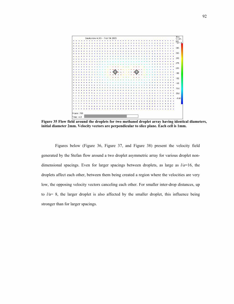
92

Figure 35 Flow field around the droplets for two methanol droplet array having identical diameters, initial diameter 2mm. Velocity vectors are perpendicular to slice plane. Each cell is 1mm.

Figures below (Figure 36, Figure 37, and Figure 38) present the velocity field

generated by the Stefan flow around a two droplet asymmetric array for various droplet non-

dimensional spacings. Even for larger spacings between droplets, as large as l/a=16, the

droplets affect each other, between them being created a region where the velocities are very

low, the opposing velocity vectors canceling each other. For smaller inter-drop distances, up

to l/a= 8, the larger droplet is also affected by the smaller droplet, this influence being

stronger than for larger spacings.

93

Figure 36 Velocity field around a two methanol droplet asymmetric array (l/a=4), a1/a2=2. Velocity vectors are perpendicular to slice plane. Each cell is 0.5mm.

Figure 37 Velocity field around a two droplet asymmetric array (l/a=8); a1/a2=2. Velocity vectors are perpendicular to slice plane. Each cell is 0.5mm.

94

Figure 38 Velocity field around a two droplet asymmetric array (l/a=16); a1/a2=2. Velocity vectors are perpendicular to slice plane. Each cell is 0.5mm.

The interactions are strong even for distances as large as l/a=40. Figure 39 and Table

14 show that the smaller droplet in the wake of the larger droplet is strongly influenced even

for spacings as large as 30 (60 when spacing is normalized to smaller droplet radius). For the

larger droplet, the correction factors for l/a between 4 and 16 are lower by 8% to 16% than

the PSM results, mainly because the radiative heat transfer lowers the temperature and,

consequently, the associated burning rates. For the smaller droplet, the effect is even stronger

for inter-drop spacings up to 50 or even larger as shown in Figure 39.

For reduced distances between droplets (l/a=4 and 8), the array behaves like the

droplets have similar diameter, almost equally influencing each other. It is the same

maximum in mass burning rates found by Mikami et al. (1994) and presented above for the

symmetric droplet array case.

95

Table 14 Correction factors and burning rates for asymmetric two droplet arrays having droplet diameters’ ratio of 2 Distance l/a1

Burning rate isolated droplet

[1E-07*kg/s]

Burning rate droplet in array

[1E-07*kg/s]

Correction factor η

PSM

Correction factor η

numerical simulation

a1 2.815 2.306 0.903 0.819 4

a2 0.669 0.554 0.774 0.828

a1 2.815 2.27 0.945 0.806 8

a2 0.669 0.545 0.882 0.815

a1 2.815 2.483 0.962 0.882 12

a2 0.669 0.551 0.920 0.824

a1 2.815 2.56 0.971 0.909 16

a2 0.669 0.556 0.939 0.831

a1 2.815 2.698 0.984 0.958 30

a2 0.669 0.601 0.967 0.898

Correction factor for an asymmetric two droplet array

0.6

0.65

0.7

0.75

0.8

0.85

0.9

0.95

1

1.05

0 10 20 30 40 50

l/a1

η

PSM η1numerical η1PSM η2numerical η2

Figure 39 Comparison between PSM and numerical solution for a two droplet asymmetric array, a1/a2=2; fuel: methanol, burning in air at atmospheric pressure and g=0

96

This phenomenon of a minimum in correction factor trend could be explained by the

effects of radiation and thermal convection: on the larger drop and on the smaller drop.

Radiation is absorbed by both droplets and does lower burning rates of droplets. However,

the smaller droplet being subjected to thermal convection generated by combustion of the

larger droplet (smaller droplet is in the wake of the larger droplet) will be exposed to two

phenomena: one is the enhancing of the gasification rate due to convection and the other is

the oxygen starvation due to combustion of the larger droplet in its vicinity. At certain

spacings between the two droplets, the enhancing of the gasification rate is predominant upon

the oxygen starvation, leading to a higher than expected burning rate for the smaller droplet.

Therefore the correction factor of the smaller droplet is higher than that predicted by PSM.

Same phenomena occur to the larger droplet, being affected by the thermal convection

generate by combustion of the smaller droplet, enhancing also the burning rate, but at a

reduced scale. As it can be observed, the correction factor for the larger droplet has also an

increased value for inter-drop spacings of 4. However, the smaller droplet is affected by the

bigger droplet, its mass burning rate being lower than the similar isolated droplet burning in

air. This phenomenon is more significant when the droplets are closer. As the droplets move

further apart, the influence of smaller droplet upon the larger one becomes less significant

and their behavior becomes similar to that obtained using PSM.

The mass burning rates for the larger drop at inter-drop distances up to 10 are

approximately 80% of the isolated drop burning rates while PSM data shows a 10% reduction

in mass burning rate for same droplet when compared to single droplet burning rate. As the

distance between droplets is increased, the smaller droplet burning rate is in the range of 80%

to 90% of the similar single droplet burning rate, while the larger drop burning rate is from

87% to 96% of isolated droplet burning rate. Compared to PSM, the numerical simulation

97

predicts more significant droplet interactions, even for very large droplet spacings. This is in

very good agreement with theoretical model of Leiroz and Rangel (1997) that predicts strong

droplet interactions for a center droplet in a large array. This result also agrees with the

experimental data of Okai et.al (2000) for a pair of methanol droplets burning in air at

atmospheric pressure under microgravity (diameters of 0.9mm ±0.15mm). Their experimental

data predicted values for K/K0 in the range of ~0.8 to ~0.5 for inter-drop spacings from 13.6

to 5.4.

For the symmetric case, the flame around the array has a cylindrical shape with

ellipsoidal ends (Figure 40), consistent with conclusions of Okai et al., 2000. For the asymmetric

case, the flame will be, for reduced distances apart, of the shape of an asymmetric ellipsoid

(Figure 41) and for larger spacings, the flame become more of a surface created by the

intersection of two pear shaped flames, posed tip to tip (Figure 42 and Figure 43). At a droplet

radii ratio of 2, the droplet pair burns as an array and not as individual droplets even for droplet

spacings up to l/a=20.

The heat release and temperature profiles for an asymmetric methanol droplet pair

shown in Figure 42 and Figure 43, indicate that even for spacings as large as 16 (l/a2=32),

both droplets interact strongly with each other with the smaller droplet being more affected.

98

Figure 40 Flame position for a two droplet symmetric array burning in air.

Figure 41 Flame contours for a two droplet asymmetric array (a1/a2=2, l/a=4)

99

Figure 42 Flame contours for a two droplet asymmetric array (l/a=16), based on heat release per unit volume.

Figure 43 Temperature profile for a two droplet array of different diameters (l/a1=16, l/a2=32).

100

5.3.3 Three Droplet Arrays: FDS_v4

We next modeled arrays containing three methanol droplets having varying droplet

diameters. To simplify the calculations of the PSM correction factors, the droplets were mounted

in the apices of a quasi-equilateral triangle. Burning rates were calculated using the same method

as for a single droplet, described in a previous section. Both symmetric and asymmetric

configurations assume that the droplets radii ratios are a1/a2=1.33 and a1/a3=2. For a symmetric

configuration, droplet sizes were 2 mm and the normalized spacings between droplets were ~6

and ~16, respectively. For asymmetric cases l/a1=~7.2, and 19.6, respectively for the same 2 mm

size droplet for the larger droplet. In descending size order, the droplets will be a1 (largest), a2 and

a3 (smallest).

The isolated droplet mass burning rates used to calculate correction factors (Table 15) are

as follows: for 2 mm diameter droplet 2.815E-7[kg/s], for 1.5 mm diameter droplet 1.41[kg/s]

and, for 1 mm droplet diameter 0.669E-07[kg/s].

For both configurations, the burning rates of the droplets in the array are decreasing by

25% for l/a=6 and by 10% to 12% for l/a = 16 or larger. Note that the normalized distance

between droplets is the ratio of the spacing between two neighboring droplets to the radius of

largest droplet. For the symmetric configuration, the numerical correction factor is in excellent

quantitative agreement with PSM.

101

Table 15 Correction factors for three methanol droplet arrays of identical or different droplet sizes

Configuration l/a Burning rate

1E-07*[kg/s]

PSM

η

Numerical

η

Experimental

η

(Liu, 2003)

6 2.181 0.75 0.774 - Symmetric

16 2.525 0.889 0.897 -

a1 2.264 0.837 0.804 -

a2 1.106 0.797 0.783 6

a3 0.498 0.761 0.745

a1 - 0.908 - 0.86

a2 - 0.888 - 0.751 12

a3 - 0.868 - 0.694

a1 2.564 0.942 0.911 -

a2 1.248 0.93 0.883 -

Asymmetric

20

a3 0.574 0.918 0.859 -

Analyzing the asymmetric configuration, the correction factors are 5% to 8% lower than

those predicted by PSM, showing stronger droplet interactions at the same droplet spacings. This

behavior is similar to that predicted by the two droplet array simulations. As shown in the Figure

44, the burning rates for the smallest droplets decrease by 12% at l/a larger than 20, and by 25%

when l/a is less than 6. Extrapolating the results for larger droplet separation distances, as the

droplet size is decreasing the effect of droplet interactions is stronger, even for droplet normalized

spacings larger than 20 (l/a = 40 when normalized with smallest droplet radius). The main

conclusion here is that no matter how large the inter-drop non-dimensional spacing is, the effect

of the larger drops upon the smallest droplet is strong. These results are in very good agreement

with those predicted by the PSM.

102

a1/a2=1.33, a1/a3=2

0.4

0.5

0.6

0.7

0.8

0.9

1

0 10 20 30 40 50l/a1

η

PSM ηsnumerical ηsPSM η1numerical η1expt. η1 (Liu, 2003) PSM η2numerical η2expt. η2 (Liu, 2003) PSM η3numerical η3expt. η3 (Liu, 2003)

Figure 44 Correction factor for a three methanol droplet arrays of equal and different droplet sizes, mounted in the apices of a triangle compared against PSM results and Liu (2003) experimental data

The experimental investigation performed by Dietrich et al (1997), shown in Figure 45,

indicates a decrease in the burning rate of the center methanol drop of only about 8% when l/a is

close to 8 (l/d=4, where “d” is droplet diameter whereas, “a” is the droplet radius). These results

also show a maximum in the burning rate at a specific value of l/a. This phenomenon was also

captured by the numerical simulation for the two droplet array as well as the experimental data of

Mikami et al (1994). As of now, there is not enough data from our numerical model for three

droplet arrays to conclude that this maximum in burning rates would occur. Further developments

of our model would have to be performed before evaluating these observations. Nonetheless, the

numerical results are following the same general trend as the data of Dietrich et al. (1997), being

in a range of 15% or less of their results.

Liu (2003) found that vaporization rates for droplets in a cluster are decrease by 15% to

30% of the single droplet values for droplet normalized spacings of 10 to 12. These results are 8%

103

to 15% lower than those predicted by PSM and 10% lower than current numerical solution, for

similar values of l/a (Figure 44). The experimental investigation of Liu (2003) studied droplet

interactions of vaporizing droplets under normal gravity, interactions being generated by the fuel

vapor concentration around the droplets while the present numerical solution investigates droplet

interactions during combustion. The explanation of the difference between the results of these

two studies could be that while one is based on vapor accumulation effects, the other is a balance

between the enhanced burning rates due to heat release and the lowering of burning rates due to

radiation and oxygen starvation effects.

Figure 45 Measurement of K/K0 ratio for a three droplet array where K is the burning rate of a center drop in a linear array and K0 is the isolated droplet burning rate (Dietrich et al., 1997)

Another aspect that was investigated was the flame shape around the droplet cluster. As

illustrated in Figure 46 - 46, the droplets are burning as a group even when the distance between

them increases to distances as large as 20 mm. The same phenomenon was observed by Nagata et

al.(2002) for arrays of seven hexanol and butanol droplets (2 mm to 2.5mm diameter) suspended

on glass fiber. They show a clear trend from external group combustion to single droplet

104

combustion with an increase in sample spacing, as shown in Figure 51. Similar to their

conclusions, as the distance increases, the flame surrounding the array tends to approach the edge

of the array with increasing droplets’ spacing (Figure 42 and Figure 43 for a two droplet

asymmetric array). When the inter-drop spacing is 6 mm, a single envelope flame encloses the

cluster throughout the combustion process. For symmetric configuration and relatively small

droplet spacings (up to 15mm), the flame has an ellipsoidal shape. As the distance is further

increased, the flame shape tends to become more of a triangular shape (from a two dimensional

point of view). For the asymmetric case, as the distance between droplets increases to 16mm, the

flame envelope shows more independent burning of the droplets, even if the droplet interactions

are still present and there is still a common flame surrounding the cluster.

The current numerical solution proved to be in very good qualitative agreement with

experimental results of Nagata et al (2002) and with the group combustion theory.

Figure 46 Flame two-dimensional contours for a three droplet symmetric array (front view) at 4.0s of simulation

105

Figure 47 Flame two-dimensional contours for a three droplet symmetric array (top view) at 4.0s of simulation

Figure 48 Three-dimensional iso-contours for 3850kW/m3 heat release per unit volume of (flame approximate position) for a symmetric three droplet array burning in air after 4.0s of simulation

106

Figure 49 Flame contours for a three droplet asymmetric array, having different droplet sizes (a1/a2=1.33, a1/a3=2, l/a1~7) at 4.0s of simulation

Figure 50 Three-dimensional iso-contours for 6300kW/m3 heat release per unit volume of (flame position) for an asymmetric three droplet array burning in air after 4.0s of simulation

107

Figure 51 Flame shape history as a function of separation distance for seven droplet two dimensionally arranged clusters of droplets (L varies from 10mm to 30 mm) (Nagata et al., 2002)

Evaluating the results of numerical simulations for two and three droplet arrays, it can be

concluded that the predictions are in excellent agreement with theoretical and experimental data

from existing literature and also that this model could be extended for droplets arrays having

more than 3 droplets. To investigate arrays with larger numbers of droplets, the configuration

should include multiple meshes around groups of droplets positioned abut to limit the number of

parameters calculated for each mesh and for time increment and thus decrease the computational

time and the likelihood of stalled calculations. The major limitation is the actual computational

resources available. Another issue is the limited number of meshes (five) that could be employed

with FDS. Under these circumstances, the model could be extended to study up to 15 droplets

108

CHAPTER 6: EXPERIMENTAL INVESTIGATION

The previous sections identified several areas of droplet interactions that could be

investigated. Numerical simulation is an approach that, while complex and time-consuming, has

been accomplished. However, interpretation of the theoretical results would benefit greatly by

experimental data obtained using similar configurations. Most previous experimental studies have

used fiber-supported droplet arrays, but the vaporization rates are generally overestimated

because of the effect of the fiber. While the effect of a supporting fiber has been analyzed for an

isolated droplet, such an analysis has not been performed for a droplet array. Given the close

proximity of the fibers in an array of fiber-supported drops, it is not reasonable to assume that the

extrapolation of the results to un-supported droplets will be the same. The presence of the fibers

has also complicated the interpretation of data from previous experiments and limited

investigations to rather small arrays.

RF Power Amplifier

Microphone Amplifier

Oscilloscope

Droplet Generator

Reflector

Positioner

Horn

Transducer

Signal Generator

Computer

Recirculating Cooler

Temperature Reading

Impedance Matching Circuit

Figure 52 Bench-top apparatus (acoustic levitator) to study evaporation of levitated fuel droplets (Liu, 2003)

To make progress in this area, an experimental configuration or technique must be developed

to reduce the effect of the droplet suspension mechanism or eliminate it altogether. To eliminate

109

the fiber, another means must be found to support the droplets. In their attempt to eliminate the

suspension fiber, some researchers used in their experiments arrays of free flying drops in a

convective stream or free falling setups to simulate the reduced gravity. The complexity of

induced by buoyancy and fibers effects should be also eliminated. A microgravity environment

would be ideal to help eliminate the effect of buoyancy.

An apparatus has been built at Drexel University’s Frederic O. Hess Engineering

Research Laboratory to study the unsupported fuel droplet evaporation and combustion (see

Figure 52 by Liu, 2003). This acoustic levitator can stabilize a two-dimensional unsupported

cluster of droplets. Using this apparatus, several sets of data were collected and it was calculated

the rate of evaporation for isolated drops, arrays of 2 drops and arrays of 3 drops through a linear

interpolation. There were obtained sets of evaporation constants K for all three configurations

mentioned above. The experimental conditions were adjusted to match the theoretical model

proposed. Also, the isolated drop experiment was performed in the similar conditions (ambient

and drop temperature and pressure, calibration, fuel used) as the 2-drop and 3-drop experiments

(Liu and Ruff, 2001).

Because of the unique nature of the apparatus to be used in this experiment, a

considerable amount of development and testing in normal gravity was required. A normal-

gravity test facility was constructed and completed at Drexel University. Specifically, two

essential development issues were overcome: (1) to design and fabricate an acoustic levitator to

stabilize a two-dimensional droplet cluster prior to combustion and (2) to develop a method to

introduce a specified number and size of droplets into the acoustic field. This facility has been

used to conduct tests of the evaporation of interacting droplets (Liu and Ruff, 2001).

110

An important step forward is to perform experiments in microgravity environments to

eliminate the effects of gravity and to reduce the influence of the acoustic field, knowing that in

microgravity the droplets will remain suspended without an acoustic field. To achieve this

objective it is necessary to build a system that will incorporate the components of the acoustic

levitator and that will meet the requirements to perform experiments in a drop-tower facility (see

Figure 53). This rig is useful to investigate many of the complex fluid mechanic and chemical

kinetic issues surrounding the combustion of clusters of drops. One of the tasks will be to study

the evaporation of drops in an array. Mirroring the previous 1-g experiments, similar sets of data

can be collected, having the advantage of more accurate data provided.

Figure 53 Drop Tower Rig System to study evaporation and combustion of unsupported fuel clusters of droplets under microgravity

111

In this experiment, the formation of the clusters can be precisely controlled using an

acoustic levitation system so that dilute and dense clusters can be created and stabilized before

combustion is begun. Therefore, this experiment will allow the spectrum of droplet interactions

during combustion to be observed and quantified. This data will provide a realistic and logical

intermediate step in the progression of experiments from individual droplet combustion to spray

flames. It will reduce the extrapolation required to extend results of droplet array studies to those

obtained in spray combustion systems. The data will also provide the needed experimental

verification of group combustion models currently being applied to complex flow situations.

6.1 Operating Parameters

The primary effects to be investigated in this proposed experiment include (1) the effect

of droplet size, cluster size and number of drops on the combustion process, (2) the effect of the

type and composition of fuel on group combustion, and (3) the ability of the group combustion

number to scale the observed group combustion regimes. Initially, only a small subset of these

will be investigated and the tests will be conducted at one atmosphere pressure. Currently, tests

are planned using clusters containing 1, 5, 10, 15, and 20 drops. These increments are selected to

compare with various droplet array studies reported in the literature. For each of these clusters,

tests will first be performed with methanol. We will first develop the test procedures using a

single levitated drop and then expand the test matrix to increasing numbers of droplets. Once

successful atmospheric tests have been achieved and the test procedures clearly defined,

modifications to the base apparatus to enhance its capabilities can be considered.

112

6.2 Description of the Test Hardware

6.2.1 Microgravity Environment

The droplets cannot be ignited in normal gravity environment because the presence of the

igniter disrupts the acoustic field. Therefore, the challenges that remained in the development of

the reduced gravity facility were to (1) develop a method to ignite the droplet cluster and (2)

assemble all of these components into a controllable experiment in a drop tower rig. The

mechanical and electrical design described in the Final Design Review document at NASA will

also briefly be presented in the following sections, and all the tables containing technical

specifications will be presented in the Appendix D.

6.2.2. Mechanical Design

A mechanical layout for the components required for this experiment has been

developed. Figure 54 and Figure 55 show top and side views of the components placed in a

standard A-frame drop rig. A list of components and the manufacturer is shown in the Appendix

D.

Acoustic Levitator

This system includes the piezoelectric transducers, the acoustic reflector, front and rear

transmitter blocks, and the reflector traverse. The droplet cluster is formed between the acoustic

driver and reflector.

113

Signal Generation

This system produces and controls the signal that operates the acoustic levitator. It

includes a programmable function generator, a signal amplifier, a step-up transformer, and a

signal generator control circuit.

Droplet Insertion

This system produces the droplet cluster in the levitator. It consists of a syringe pump,

a needle positioner motor, and a high voltage power supply. The syringe pump and needle

positioner introduce a droplet into the acoustic field while the high voltage power supply is used

to break up the ‘parent’ droplet and form the cluster. Methanol and ethanol will be used for the

initial tests.

Igniter Assembly

This system moves and controls the igniter and igniter motion. It consists both of the

igniter traverse, hot wire, and an elevator that drops the igniter out of the plane of the droplet

cluster.

Diagnostics

Two color CCD cameras form the primary diagnostics for this experiment. The

droplets are illuminated from the side by an LED. One camera looks at a backlit image of the

cluster while the other looks down on the cluster through the reflector. Thermocouples are used to

monitor the ambient temperature inside the enclosure and of the acoustic transmitter.

114

General

The levitator and needle positioner are located inside an enclosure. This is a non-sealed

volume intended to acoustically isolate the acoustic levitator and provide a still ambient

environment during the drop. The purge bottle is present so that the contents of the enclosure can

be purged to the drop tower vent system after each drop.

As shown in Figure 54 and Figure 55, the batteries are placed at the bottom of the rig

along with the base for the acoustic levitator. A second level from the bottom holds the

components for the signal generation system, i.e., the power amplifier, signal generator and

transformer, and box for the control circuit. The fuel syringe and motor, stepper motor control

box and high voltage power supply are mounted on a second shelf at the level of the droplet

array. The side-view camera and the diagnostic control box are also mounted on this shelf. The

droplet array is viewed from the side and the top through a window in the center of the reflector.

The power distribution module, computer control system, and relay box and DC-AC converter

are shown placed on the top of the rig.

While Figure 54 and Figure 55 show the general layout of the rig, the detail of the

components inside the enclosure is not well represented. The components contained inside the

enclosure are:

• igniter and elevator assembly

• acoustic reflector

• reflector traverse motor and assembly

• thermocouples (air, acoustic levitator)

• needle traverse

115

A schematic of the layout of the components inside the enclosure is shown in Figure 56. The

igniter assembly has been designed and is shown in Figure 57. Figure 58 shows detail of the loop

igniter assembly. This component has been fabricated at NASA Glenn Research Center and is

currently undergoing testing. The acoustic reflector, reflector traverse, and needle traverse will be

mounted onto the igniter and elevator assembly.

116

Signal Generator

Ther

moc

oupl

eIn

terfa

ce B

ox

0 5 10 15 20 25 30 35 38

0

5

10

15

Fiber OpticTransmitter 2

24 VDC Battery BoxIgniterAssembly 24 VDC Battery Box

Signal Amplifier

Fiber OpticTransmitter 1

Signal GenControl Box

Stepper MotorControl Box

High VoltagePower Supply

Power Distribution

Module

TT8-DDACSTransformerCircuit BoxCameraLens

PurgeBottle Fuel Syringe and Motor

LED Control Box

Relay Box

Enclosure

Signal Generator

Ther

moc

oupl

eIn

terfa

ce B

ox

0 5 10 15 20 25 30 35 380 5 10 15 20 25 30 35 38

0

5

10

15

0

5

10

15

Fiber OpticTransmitter 2Fiber Optic

Transmitter 2

24 VDC Battery BoxIgniterAssembly 24 VDC Battery Box

Signal Amplifier

Fiber OpticTransmitter 1Fiber Optic

Transmitter 1Signal GenControl Box

Stepper MotorControl Box

High VoltagePower Supply

Power Distribution

Module

Power Distribution

Module

TT8-DDACSTransformerCircuit BoxCameraLens CameraCameraLensLens

PurgeBottle Fuel Syringe and Motor

LED Control Box

Relay Box

EnclosureEnclosure

Figure 54 Mechanical lay-out of the Droplet Cluster Rig (top view)

117

0

5

10

15

20

25

30

33

0 5 10 15 20 25 30 35 38

IgniterAssembly

24 VDC Battery Box

Cam

era

Lens

Power Distribution Module

Fiber OpticTransmitter 1

24 VDC Battery Box

Fiber OpticTransmitter 2

TT8-DDACS

ThermocoupleInterface Box

Signal Generator

Stepper MotorControl Box

Signal GenControl Box

TransformerCircuit Box

High VoltagePower Supply

Fuel Syringe and Motor

CameraLens

PurgeBottle

Signal Amplifier

Relay Box

DC-AC InverterLED Control Box

0

5

10

15

20

25

30

33

0

5

10

15

20

25

30

33

0 5 10 15 20 25 30 35 38

IgniterAssembly

24 VDC Battery Box

Cam

era

Lens

Cam

era

Cam

era

Lens

Lens

Power Distribution ModulePower Distribution Module

Fiber OpticTransmitter 1Fiber Optic

Transmitter 1

24 VDC Battery Box

Fiber OpticTransmitter 2Fiber Optic

Transmitter 2

TT8-DDACS

ThermocoupleInterface BoxThermocoupleInterface Box

Signal Generator

Stepper MotorControl Box

Signal GenControl Box

TransformerCircuit Box

High VoltagePower Supply

Fuel Syringe and Motor

CameraLens CameraCameraLensLens

PurgeBottlePurgeBottle

Signal Amplifier

Relay Box

DC-AC InverterLED Control Box

Figure 55 Mechanical lay-out of the Droplet Cluster Rig (side view)

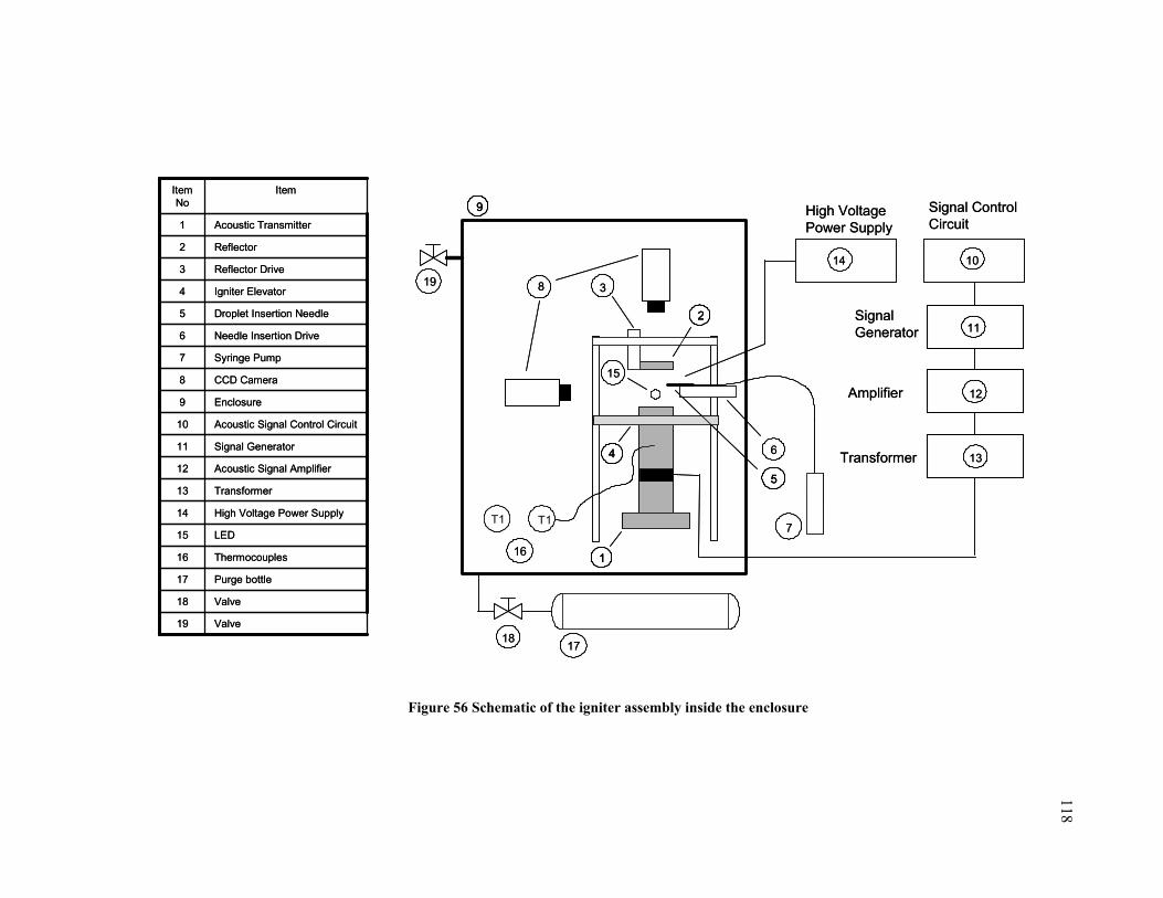
118

SignalGenerator

Amplifier

Transformer

1

Signal ControlCircuit

High VoltagePower Supply

2

3

4

5

11

6

10

13

7

8

9

15

12

14

16

T1 T1

1718

19

SignalGenerator

Amplifier

Transformer

11

Signal ControlCircuit

High VoltagePower Supply

22

3

44

55

11

6

10

13

7

8

99

15

12

14

16

T1T1 T1T1

1718

19

Figure 56 Schematic of the igniter assembly inside the enclosure

Valve19

Valve18

Purge bottle17

Thermocouples16

LED15

High Voltage Power Supply14

Transformer13

Acoustic Signal Amplifier12

Signal Generator11

Acoustic Signal Control Circuit10

Enclosure9

CCD Camera8

Syringe Pump7

Needle Insertion Drive6

Droplet Insertion Needle5

Igniter Elevator4

Reflector Drive3

Reflector2

Acoustic Transmitter1

ItemItem No

Valve19

Valve18

Purge bottle17

Thermocouples16

LED15

High Voltage Power Supply14

Transformer13

Acoustic Signal Amplifier12

Signal Generator11

Acoustic Signal Control Circuit10

Enclosure9

CCD Camera8

Syringe Pump7

Needle Insertion Drive6

Droplet Insertion Needle5

Igniter Elevator4

Reflector Drive3

Reflector2

Acoustic Transmitter1

ItemItem No

119

Figure 57 Igniter elevator assembly

120

Figure 58 Loop igniter assembly

121

6.3. Test Procedures

The entire experimental investigation will be conducted at the 2.2 Second Drop Tower at

NASA Glenn Research Center. The operation of this experiment is best explained using the

experiment timeline shown in Figure 59. The drop tower will be prepared for a drop with the

experiment package enclosed in the drag shield and positioned at the top of the tower. At this

time, electrical connections will still be in place so an external operator can control the formation

of the droplet cluster.

First, the acoustic field will be initiated by turning on the power amplifier. The operator

will then dispense a specified amount of fuel to the tip of the hypodermic needle and the reflector

traversed to form the droplet cluster in the acoustic field. The droplet generator will be retracted.

After the operator verifies that a stable cluster has been formed, he will initiate automated control

of the experiment. (The formation of the cluster will be verified visually using the on-board CCD

camera.) If an external connection has been used for initial experiment control, it will be detached

at this time. The facility operators will then be notified that the rig is prepared to drop.

The acoustic field will be turned off when the computer receives the drop initiation

signal. It is unclear whether it will be best to terminate the field instantly or to more gradually

decrease the levitating force. The igniters will also be energized and, after a specified time,

retracted so they don’t interfere with the cluster during the drop. In any event, the timing for the

removal of the acoustic field and energizing of the igniters will be controlled by the computer and

are variables that will be worked out during the first checkout drops. The experiment will proceed

and data collected until the end of the drop, at which time all systems will be de-energized.

This timeline is also described in Table 18 from Appendix D in terms of the experiment

control actions.

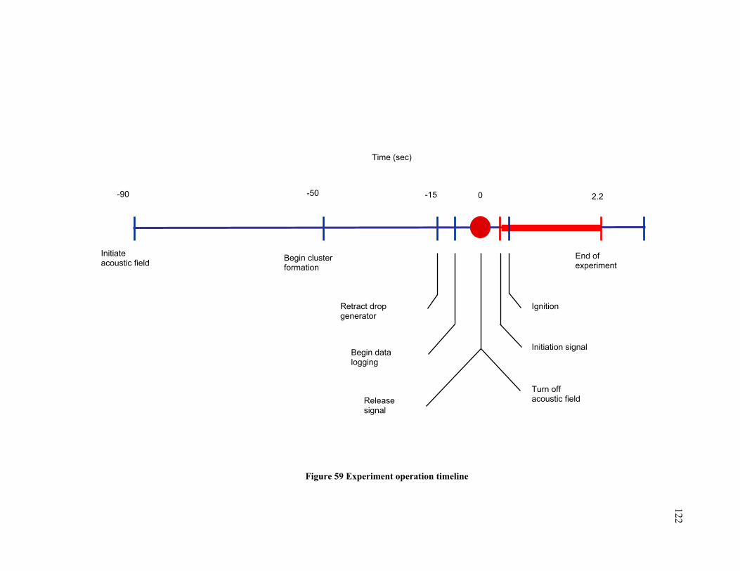
122

Figure 59 Experiment operation timeline

-15 0 2.2 -90

Release signal

Initiation signal

Turn off acoustic field

Time (sec)

-50

Retract drop generator

End of experiment

Begin data logging

Ignition

Begin cluster formation

Initiate acoustic field

123

CHAPTER 7: SUMMARY AND RECOMMENDATIONS

The present work developed a numerical model to study the combustion of well-

characterized drop clusters in microgravity environment using direct numerical simulation. The

computational research investigated the combustion of clusters of droplets of different sized and

asymmetric three-dimensional configurations in zero gravity environments for zero relative

Reynolds numbers. One of the aspects studied is droplet interaction during evaporation and

combustion over the lifetime of the droplet. The model proved to be able to provide reliable data

that will support future microgravity experimental investigations.

Background and Motivation

In general, isolated droplet investigations are not amenable to the analysis of arrays of

drops or clusters because of the complexity of the methods used and the effect of the gaseous

environment and drop-drop interactions. The study of isolated droplets has revealed aspects of

droplet behavior that have aided the development of investigations using arrays of drops. These

findings include that the evaporation rates are strongly affected by (1) the heat conduction

induced by a supporting fiber, (2) radiative absorption, (3) the ambient temperature and pressure,

(4) buoyancy, and (5) the Re, Sh and Nu numbers.

In an array or cluster of drops, a drop is affected by its nearest neighboring droplets. In

the analysis of an array of droplets, droplet interactions are considered. The proximity of a

neighboring droplet affects the mass and energy transfer between the droplet and the surrounding

gas, the lift and drag coefficients and the Nusselt and Sherwood numbers. Droplet interactions are

strongly affected by the Reynolds number and they are dependent on the geometry of the array.

124

The effect of the fiber on droplet interaction and droplet vaporization and combustion

phenomena has not been studied for arrays of fiber-supported drops because the cumulative effect

of the fibers would eventually mask the details of droplet behavior. Furthermore, this type of

analysis would require a large amount of time and computational resources. Droplet interactions

for non-symmetric and larger arrays of drops can be large and should also be investigated. The

effect of the Reynolds number on interacting droplets is an important issue that has been

investigated both through analytic and numerical methods. Unfortunately, for low Reynolds

numbers, experimental studies are not available yet. The investigation of unsupported arrays of

drops for near zero Reynolds numbers, both theoretical and experimental, could offer a better

understanding of the droplet interaction phenomena.

Point Source Method

The Point Source Method investigates the effect of droplet interactions for arrays up to

1000 droplets, arranged in symmetric configurations, evaluating the mass loss rate of interacting

drops, under quasi-steady and quiescent atmosphere. The method accounts for variable thermo-

physical properties. PSM is valid only if l/a>>1. The Point Source Method has been verified

against data provided by current theories but there are no comparisons with experimental data. An

extension of a current theory (Point Source Method) has been investigated for non-symmetric

two- and three-drop arrays. Droplet interactions have been evaluated using the ratio of the

vaporization rate in an array to an isolated drop that defined the correction factor.

The PSM results led to the conclusion that droplet interactions are strong for non-

dimensional inter-drop spacings between 2 and 20 (for configuration using drops with similar or

near similar diameters). As the spacing between droplets increases, droplet interactions are

weaker. For small droplets in the wake of a larger drop, droplet interactions are present and strong

125

even for large inter-spacing (up to l/a~50). The evaporation rate of the smaller drops could

decrease by up to 30-40% compared to an isolated drop.

Model Description and Problem Formulation for Numerical Solution

A three dimensional model of symmetric and asymmetric arrays of fuel droplets burning

under microgravity conditions have been developed, that will mimic (as close as possible) the

experimental model allowing the spectrum of droplet interactions during combustion to be

observed and quantified. The particularity of this numerical simulation is that each drop in the

array vaporizes and burn according to the conditions created by the environment around the

droplet and also the array can be considered as an entity.

The model study accounts for radiative heat transfer using a Finite Volume Method,

Stefan convection, diffusion and finite-rate chemical kinetics, a quiescent environment, near zero

Reynolds number, and gas-phase variable thermo-physical properties and unity Lewis number but

does not account for forced convection and for internal circulation within the droplet.

The numerical solution is based on Fire Dynamic Simulator, computational fluid dynamic

numeric model of thermally-driven fluid flow that solves Navier-Stokes equations for low-speed

flow. The combustion model assumes one-step chemical reaction. Spatial and temporal

discretization is based on rectilinear three dimensional grids and a time step increment adjusted

according to von Neumann criterion.

Initially, a modified version of FDS_v3, which included a radiation solver for finite-rate

reaction combustion, was used and preliminary results were in good qualitative agreement with

PSM and other theoretical data for combustion of single drop and arrays of drops. Later during

the project development the simulations were performed using FDS_v4, based on the advantages

126

offered by new version of FDS, including but not limited to a finite volume fraction solution of

radiation equation for finite-rate reaction model, a faster solution and reduced CPU time.

Mass burning rates are calculated using a numerical algorithm using the output data

provided by FDS_v4 and a non-dimensional factor η (defined similar to PSM) was calculated to

account for droplet interactions. Several cases were investigated to determine the ignition times

and the necessary ignition energy to sustain the combustion. As a conclusion, it was determined

that the ignition time required for methanol to reach flame temperature was 2s to 2.5s, using four

igniters positioned at one cell apart from the droplet and having a wall temperature of at least

3000ºC.

Validation of the Code Using Isolated Droplet Combustion

Both sensitivity and validation has been performed using a single droplet configuration,

the numerical results being compared to the theoretical and experimental data found in literature.

Several factors have been studied for single droplet combustion before investigating the

combustion of multiple droplets, such as the sensitivity of temperature and burning rates to

domain size and grid size (number of cells into a domain and cell size). For single droplet

combustion, as the domain increases in size, the combustion parameters become independent of

the domain size and burning rates for dimensions larger than 403mm. If a finer grid is used, the

burning rates are not as sensitive to the domain size.

The burning rates were found to be affected by the grid size, and less by the domain size

(slightly more affected for small computational domains); therefore a grid size that satisfies the

ignition condition has been employed for the simulation of clusters of droplets. Combustion

parameters for two and three droplet arrays become domain independent for a domain size larger

127

than 403mm. If the distance between droplets increases, the domain size has to be increased

accordingly.

Varying the oxygen concentration in the ambient surroundings from 10% to 75% by

volume the numerical results (burning rates and flame positions during combustion) are in good

qualitative agreement with numerical and experimental data obtained by Marchese and Dryer

(1999), being in the range of 10% of their result-and data plotted following similar trends.

Turning on and off the radiation solver, the numerical model predictions shows a

reduction in mass burning rates when radiation is considered being in good qualitative agreement

with the model developed by Marchese et al. (1999) for a 5 mm isolated pure methanol droplet

and also with the numerical and experimental results of Kumagai (1971) and King (1996) for a

0.98mm n-heptane burning droplet. Burning rates without non-luminous radiation will become

grid and domain independent for larger domains and finer grids that those cases with non-

luminous radiation considered. The flame diameter for a 1 mm droplet burning in air with and

without non-luminous radiation considered is in good quantitative and qualitative agreement with

experimental and numerical data of Kumagai (1971) and King (1996).

After evaluating the sensitivity and validation tests, we may conclude that the predictions

of combustion parameters by the numerical model for single droplet are in very good qualitative

agreement with theoretical and experimental results presented in the literature. The model is

amenable for analysis and prediction of mass burning rates in a reasonable margin of error (less

than 10%) for an adequately grid resolved domain. Single droplet combustion predicted by the

code follows the d2-law. The predicted data confers confidence that combustion parameters

resulted adequately characterize the combustion process of single and multiple droplets.

128

Multiple Droplet Combustion

The next step was evaluation of combustion of multiple droplet arrays under zero-gravity

conditions. Two and three droplet arrays of identical or different sizes were investigated,

increasing gradually the distance between droplets in the array.

For two droplet array configuration, the correction factors determined from the numerical

model are lower by about 10% than those predicted by PSM but 5% to 10% higher than those

predicted by the numerical model of Leiroz and Rangel (1997) for non-dimensional distances

between droplets greater than 10. For droplet spacings of l/a greater than 4, the mass burning

rates increase gradually as l/a increases, which is consistent with experimental findings of Okai et

al. (2000) for a pair of pure methanol droplets burning at atmospheric pressure under

microgravity conditions. As the normalized spacing between droplets is further reduced, burning

rates tend to slightly increase, consistent with experimental data of Mikami et al. (1994) for a n-

heptane droplet array, but contradicted by experimental findings of Okai et al. (2000) for a 0.9

mm methanol droplet. In the latter work, a minimum burning time (maximum in burning rates)

was not observed and justified by the absence of the soot in methanol combustion. Additional

investigation will be needed to clarify this issue.

An explanation of the enhancement of the burning rates for very small distances between

droplets could relay on the larger size of the droplets employed by our numerical simulations that

yields on a stronger radiative effects.

For the asymmetric case, droplet interactions are even stronger than those predicted by

PSM, the smaller droplet being more affected by the bigger droplet. Droplet interactions are

present and strong even for normalized distances between droplets greater than 50.

129

The flame envelope has a quasi-cylindrical shape, consistent with Okai et al. (2000)

conclusions for a two droplet array.

The next configuration studied was a three droplet array, with similar or different droplet

sized, and mounted in the apices of a triangle. Analyzing the asymmetric configuration, the

correction factors are 5% to 8% lower than those predicted by PSM, showing stronger droplet

interactions at same droplet spacings, being similar to that predicted by the two droplet array

simulations. The burning rates for the smallest droplets decreases by as much as 12% for l/a

larger than 20, and by as much as 25% compared to isolated droplet burning rate when l/a is

decreasing up to 6. The general behavior is following the trend of PSM results, the current

numerical solution being in very good agreement with PSM. Mass burning rates are generally

15% lower than those predicted by the experimental data of Dietrich et al. (1997). However, the

numerical data are in good qualitative agreement with experimental results of Liu (2003) and

Dietrich et al. (1997).

Varying the distance between droplets, the numerical solution predicted a flame envelope

variation consistent with experimental results of Nagata et al (2002).

The predictions of the numerical simulations are in excellent agreement with theoretical

and experimental data from literature and also that this model could be extended for droplets

arrays having more than 3 droplets. Due to limitation the actual computational resources

available, the current model could be extended to study up to 15 droplets. Further developments

to our model as well as to FDS have to be made to increase even more the number of droplets in

the cluster.

130

The model was proven to be able to investigate different array configurations to predict

the behavior of cluster of droplets. Therefore the model could mimic future experimental

configurations and provide numerical data to support experimental results.

Recommendations

As described previously in Chapter V and above in the summary section, as the droplets

in an array are closer one to each other, a maximum in burning rates has been noticed for both

two and three droplet arrays, being consistent with Mikami (1994) findings for a two droplet

array and with Dietrich (1997) experimental results for a three droplet linear array. However,

these results are contradicted by experimental findings of Okai et al. (2000) for 0.9 mm methanol

droplets, where a maximum in burning rates was not observed. Stronger radiative effects due to

larger droplets employed could explain this phenomenon. To further explore this problem, several

simulations will be needed for non-dimensional spacings slightly smaller and larger than the

inter-drop spacing for which the maximum has been found, as well as different spatial

configurations of cluster of droplets having diameters varying from 0.5mm to 4 mm should be

studied to clarify for what type of configurations this maximum in burning rates occurs. Also, an

experimental investigation of similar configurations as in the numerical study will be necessary to

validate the numerical data.

Imposing a zero Reynolds number for the numerical solution was justified by the relative

motion of the droplets in the cluster and also to match a potential experimental investigation

described previously. For intermediate and high Reynolds numbers the theoretical study of

particle interaction becomes more complex due to the necessity of taking into account the

influence of the non-linear terms of the Navier–Stokes equations on the hydrodynamic interaction

forces. Numerical approaches were used for describing the particle interactions in the non-zero

131

Reynolds numbers regime: Tal et al. (1983), Kim et al. (1993), Raju and Sirignano (1990), Tsai

and Sterling (1990), Chiang and Sirignano (1993), Liang et al. (1996), among others.

It still remains to be determined that gas phase radiative losses have a significant impact

when droplets are exposed to a slow convective flow field in microgravity. There has been little

work showing the effects that a slow convective flow field will have on the radiative heat loss and

implicit on droplet interactions for a droplet cluster burning in microgravity. An interesting

approach will be to perform similar investigation when Reynolds numbers are low, but not zero.

This could be done using the same computational code and geometrical configurations as in the

zero Reynolds case, imposing in the computational domain a convective environment: a flow of

air through one of the boundary walls that has a specified velocity.

An experimental apparatus developed at Drexel University and currently being installed

in a drop tower experiment at NASA Glenn Research Center can provide data on the behavior of

droplet clusters without the effects of fibers or buoyancy.

An important step forward is to perform similar experimental investigations in

microgravity environment to those performed in one-g, to eliminate the effects of gravity and to

reduce the influence of the acoustic field.

The numerical simulation along with the future proposed experiment described in the

project is a unique combination of investigative methods that will provide support for future

investigations and for understanding of droplet interaction phenomena.

132

LIST OF REFERENCES

Annamalai, K., Ryan, W “Evaporation of Arrays of Drops Using the Point Source Method”, ASME Publications, Emerging Energy Technology, PD, vol. 50, 1993

Annamalai, K., Ryan, W. “Evaporation of Multicomponent Drop Arrays”, Journal of Heat Transfer, vol.115, 1993

Annamalai, K, “Mechanics and Combustion of Droplets and Sprays”, (3rd Edition), New York, Begell House, 1995

Avedisian, C. T., G. S. Jackson, G.S. “Soot Patterns around Suspended N-Heptane Droplet Flames in a Convection-free Environment”, Journal of Propulsion Power 16 (6), 974-979, 2000

Brzustowski, T. A., Twardus, E. M., Wojcicky, S., and Sobiesiak, A., “Interaction of Two Burning Fuel Droplets of Arbitrary Size”, American institute of Aeronautics and Astronautics Journal, 17, pp. 1234-1242, 1979

Bergeron, C. A., Hallett, W. L. H. “Ignition Characteristics of Liquid Hydrocarbon Fuels as Single Droplets”, Can. J. Chem, Engng 67, 142-149, 1989

Chai, J. C., Patankar, S. V. “Finite Volume Method for Radiation Heat Transfer”, Journal of Thermophysics and Heat Transfer, vol. 8, pp 419-425, 1994

Chauveau, C., Chesneau, X. and Gokalp, I., “High-pressure Vaporization and Burning of Methanol Droplets in Reduced Gravity”, Adv. Space. Res. Vol 16, No.7, pp (7) 157-160, 1995

Chiang, C. H., Sirignano, W. A., “Interacting, Convecting, Vaporizing Fuel Droplets with Variable Properties”, International Journal of Heat and Mass Transfer, 36, No.4, pp. 875-886, 1993

Chiang, C. H., Sirignano, W. A., “Axisymmetric Calculations of Three-Droplet Interactions”, Atomization and Sprays, 3, pp. 91-107, 1993

Ciobanescu, I., Ruff, G. A. “Combustion of Unsupported Droplet Clusters in Microgravity”, Work-in progress Poster, Proceedings of the 30th International Symposium of Combustion Institute, July 2004

Crowe, C.T., Sharma, M.P. and Stock, D.E. “The Particle-Source-In Cell (PSI-CELL) Model for gas-Droplet Flows”, Journal of Fluids Engineering, June 1977

Cuoci, A., Mehl, M., Buzzi-Ferraris, G., Faravelli, T., Manca, D., and Ranzi, E. “Autoignition and Burning Rates of Fuel Droplets under Microgravity”, Combustion and Flame, June 2003

Daif, A., Bouaziz, M., Chesneau, X., and Cherif, A. “Comparison of Multicomponent Fuel Droplet Vaporization Experiments in Forced Convection with the Sirignano Model”, Experimental Thermal and Fluid Science, 18, pp. 282-290, 1999

133

Delplanque, J.P., Rangel, R. H., “Droplet Stream Combustion in the Steady Boundary Layer Near a Wall”, Combustion Science and Technology, 78, pp. 97-115, 1991

Delplanque, J. P., Sirignano, W. A., “Numerical Study of the Transient Vaporization of an oxygen droplet at Sub and Super-critical Conditions”, The International Journal of heat and Mass Transfer, 36, No. 2, pp. 303-314, 1993

Delplanque, J. P., Sirignano, W. A., “Boundary Layer Stripping Effects on Droplet Transcritical Convective vaporization”, Atomization and Sprays, 1994

Dietrich, D.L. et al. “Combustion of Interacting Droplet Arrays in a Microgravity Environment”, Proceedings of the Sixth International Microgravity Combustion Workshop, pp. 193-196, 2001

Dietrich, D. L., Haggard, J. B. et al., “Droplet Combustion Experiments in Spacelab”, Twentieth Sixth Symposium (International) on Combustion, The Combustion Institute, Pittsburgh, PA, pp 1201-1207, 1996

Dietrich, D. L., Struk, P. M., Kitano, K., Ikeda, K., Honma, S., “Combustion of Interacting Droplet Arrays in a Microgravity Environment”, NASA Center for AeroSpace Information (CASI) Fourth International Microgravity Combustion Workshop, NASA-CP-10194, 479-484, May 1997

Dunn-Rankin, D., Sirignano, W. A, Rangel, R. H. and Orme, M. E. “Droplet Arrays and Streams” Proceeding of the Mechanics and Combustion of Droplets and Sprays Symposium, Tainan, Taiwan, December 1994

Dwyer, H.A., Stapf, P. and Maly, R. “Unsteady Vaporization and Ignition of a Three-dimensional Droplet Array”, Combustion and Flame 121:181-194, 2000

Faeth, G. M. “Evaporation and Combustion of Sprays”, Prop. Energy Combust. Sci. 9, pp. 1-76, 1983

Faeth, G.M. “Current Status of Droplet and Liquid Combustion”, Progr. Energy Combust. Sci. 3, pp. 191-224, 1997

Faeth, G.M., Olson D. R., “Ignition of Hydrocarbon Fuel Droplets in Air”, Trans. SAE, 1793, 1968

Grosshandler, W. “RADCAL: A Narrow Band Model for Radiation Calculations in a Combustion Environment”, NIST Technical Note TN 1402, 1993

Handbook of Chemistry and Physics, 85th Edition, 2004-2005, http://www.hbcpnetbase.com.ezproxy.library.drexel.edu/

Hara, H., Kumagai, S., “Experimental Investigation of Free Droplet Combustion under Microgravity”, Twenty-third Symposium (International) on Combustion, The Combustion Institute, Pittsburgh, PA, pp 1605-1610, 1990

Hicks, M.C., Nathan, K., Easton, J., and Forman, W. A. (2003) “Radiative Heat Loss Measurements during Microgravity Combustion in a Slow Convective Flow, Third Joint Meeting of the U.S. Sections of the Combustion Institute, March 2003

134

Hollander, W., Zaripov, S. K., “Hydrodynamically Interacting Droplets at Small Reynolds Numbers”, International Journal of Multiphase Flow, vol. 31, 2005.

Howell, J., Siegel, R., “Thermal Radiation Heat Transfer”, 4th Edition, Taylor and Francis 2002

Imaoka, R.T., Sirignano, W.A. “Fuel-Droplet array Burning with Asymmetry and Droplet Size Variation”, Proceedings of Triple-Joint Meeting of Combustion Institute, March 2005

Kadota, T., Hiroyasu, H. “Evaporation of a Single Droplet at Elevated Pressures and Temperatures”, Trans. JSME 19 (138) 1515-1521, 1976

King, M. K. Twentysixth Symposium (International) of Combustion Institute, Proc. of Combustion Institute 26, 1227, 1996

Kozyrev, A. V., Sitnikov, A. G. “Evaporation of a Spherical Droplet in a Moderate-Pressure Gas”, Uspekhi Fizicheskikh Nauk, Russian Academy of Sciences, 171 (97) 765-774, 2001

Kumagai, S., Isoda, H., “Combustion of Fuel Droplets in a Falling Chamber”, Sixth Symposium (International) on Combustion, Reinhold, NY, pp 726-731, 1957

Kumagai, S. Sakai, T. and Okajihama, S., “Combustion of Free Fuel Droplets in a Freely Falling Chamber”, Thirteen Symposium (International) on Combustion, The Combustion Institute, Pittsburgh, PA, pp 779-785, 1971

Kuo, K. K. “Principles of Combustion”, Wiley & Sons, New York, 1986

Labowsky, M., “A Formalism for Calculating the Evaporation Rates of Rapidly Evaporating Interacting Particles”, Combustion Science and technology, 18, pp145-151, 1978

Labowsky, M., “Calculation of Burning Rates of Interacting Fuel Droplets”, Comb. Sci. Technol. 22, 217-226, 1980

Lage, P. L. C., Rangel, R. H., “Single Droplet Vaporization Including Thermal Radiation Absorption”, J. Thermophys. Heat Transfer 7, 502-509, 1993

Lage, P. L. C., Rangel, R. H., “Total Thermal Radiation Absorption by a Single Spherical Droplet”, J. Thermophys. Heat Transfer 7, 101-109, 1993

Law, C. K., “Unsteady Droplet Combustion with Droplet Heating”, Combustion and Flame, 26, pp. 17-22,1976

Law, C. K., Sirignano, W. A., “Unsteady Droplet Combustion with Droplet Heating-II: Conduction Limit”, Combustion and Flame, 28, pp. 175-186, 1977

Law, C. K., “Recent Advances in Droplet Vaporization and Combustion”, Progress in Energy and Combustion Science, vol. 8, pp 171-201, 1982

Leiroz, A., Rangel, R.H., “Numerical study of Droplet-Stream Vaporization at Zero Reynolds Number”, Numerical Heat Transfer. Part A, Applications. 27, no. 3, 273, 1995

135

Liu, S. “Formation, Evaporation and Microgravity Combustion of Unsupported Liquid Fuel Droplet Cluster”, Drexel University, Doctoral Thesis, 2003

Malahan, J. R., “Radiation Heat Transfer: A Statistical Approach”, John Wiley & Sons, New York, 2002

Marberry, M., Ray, A. K., and Leung, K., “Effect of Multiple Particle Interactions on Burning Droplets”, Combustion and Flame, 57, pp. 237-245, 1984

Marchese, A. J., Dryer, F. L., “The Effect of Liquid Mass Transport on the Combustion and Extinction of Bi-Component Droplets of Methanol and Water”, Combust. Flame 105, pp. 104–122, 1996

Marchese, A.J., Dryer, F.L., “Science Support For Space-Based Droplet Combustion: Drop Tower Experiments and Detailed Numerical Modeling, Princeton University, Department of Mechanical and Aerospace Engineering (website)

Marchese, A.J., Dryer, F.L., and Nayagam, V. “Numerical Modeling of Isolated N-Alkane Droplet Flames: Initial Comparisons with Ground and Space-Based Microgravity Experiments”, Combustion and Flame 116, pp. 432–459, 1999

McGrattan, K., “Fire Dynamic Simulator (Version 4) – Technical Reference Guide”, NIST Special Publication 1018, 2005

McGrattan, K., Forney, G. “Fire Dynamic Simulator (Version 4) – Users Guide”, NIST Special Publications 1019, 2005

Megaridis, C.M., Sirignano, W.A., “Numerical Modeling of a Slurry Droplet Containing a Spherical Particle”, Journal of Thermophysics and Heat Transfer, vol 7, 1993

Mikami, M., Habara, O., Kono, M., Sato, J., Dietrich, D. L., and Williams, F. A., “Pressure Effects in Droplet Combustion of Miscible Binary Fuels” NASA Center for AeroSpace Information (CASI), Fourth International Microgravity Combustion Workshop, NASA-CP-10194, 497-502, May 1997

Mikami, M., Oyagi, H., Kojima, N. et al., “Microgravity Experiments on Flame Spread Along Fuel-Droplet Arrays Using A New Droplet-Generation Technique”, Combustion and Flame vol. 141, 2005.

Minkowycz, W. J., Sparrow, E. M., “Advances in Numerical Heat Transfer”, vol. II, Taylor and Francis, 2000

Moriuea, O., Mikami, M., Kojima, N., and Eigenbrod, C., “Numerical Simulations of the Ignition of N-Heptane Droplets in the Transition Diameter Range from Heterogeneous to Homogeneous Ignition”, Proceeding of the Combustion Institute 30, 2005.

Murthy, J. Y., Mathur, S. R., “Finite Volume Method for Radiation Heat Transfer Using Unstructured Meshes”, Journal of Thermophysics and heat Transfer, vol. 12, pp 313-321, 1998

136

Nagata, H., Kudo, I., and Nakamura, S., “Interactive Combustion of Two-dimensionally Arranged Quasi-droplet Clusters under Microgravity”, Combustion and Flame vol. 129, 2002

Nguyen, Q. V., Rangel, R. H., and Dunn-Rankin, D., “Measurement and Precision of Trajectories and Collision of Droplets”, International Journal of Multiphase Flow, 17, pp. 159-177, 1991

Nguyen, Q. V., Dunn-Rankin, D., “Experiments Examining Drag in Linear Droplet Packets”, Experiments in Fluids, 12, pp. 157-165, 1992

Okai, K, Moriue, O., Araki, M., Sato, J. Dietrich, D. L., and Williams, F. A., “Pressure Effects on Combustion of Methanol and Methanol/Dodecanol Single Droplets and Droplet Pairs in Microgravity”, Combustion and Flame vol.121, 2000

Patnaik, G., Sirignano, W. A., Dwyer, H. A. and Sanders, B. R., “A Numerical Technique for the Solution of a Vaporizing Fuel Droplet”, Dynamics of Reactive Systems, Progress in Astronautics and Aeronautics, 105, AIAA, pp. 253-266, 1986

Perry’s Chemical Engineering Handbook (e-book), “Interactive Tables of Organic and Inorganic Compounds”, http://www.hbcpnetbase.com.ezproxy.library.drexel.edu/

Raithby, G. D., Chiu, E. H., “A Finite Volume Methode for Predicting Radiant Heat Transfer in Enclosures with Participating Media”, Journal of Heat Transfer, 112 (2): 415-423, 1990

Raju, M. S., Sirignano, W. A., “Interaction between Two Vaporizing Droplets in an Intermediate-Reynolds-Number-Flow”, Physics of Fluids, 2, pp. 1780-1796, 1990

Rangel, R. H., Sirignano, W. A. “An Evaluation of the Point Source Approximation in Spray Calculations”, Numerical heat Transfer, Part A, vol. 16, pp. 35-57, 1989

Ross, H. “Microgravity Combustion: Fire in Free Fall”, Academic Press, 2001

Ruff, G.A., Liu, S. “Combustion of Unconfined Droplet Clusters in Microgravity”, Proceedings of the Sixth International Microgravity Combustion Workshop, pp. 389-392, May 2001

Ruff, G.A., Liu, S., and Ciobanescu, I. “Vaporization and Combustion of Unconfined Droplet Clusters in Microgravity”, Proceedings of the Seventh International Microgravity Combustion Workshop, pp.5-8, 2003

Saitoh, T., Yamazaki, K. and Viskanta, R. “Effect Of Thermal Radiation on Transient Combustion of a Fuel Droplet”, J. Thermophys. Heat Transfer 7, 94-100, 1993

Sangiobanni, J. J., Labowsky, M., “Burning Times of Linear Fuel Droplet Arrays: A Comparison of Experiment and Theory”, Combustion and Flame, 47, pp. 15-30, 1982

Shih, A. T., Megaridis, C. M. “Suspended Droplet Evaporation Modeling in a Laminar Convective Environment”, Combustion and Flame 102: 256-270, 1995

Siegel, R., Howell, J. “Thermal Radiation Heat Transfer” (4th Ed.), Taylor and Francis, New York

137

Sirignano, W. A., “Fuel Droplet Vaporization and Spray Combustion Theory”, Progress in Energy and Combustion Science, vol. 9, pp 291-322, 1983

Sirignano, W. A., “Fluid Dynamics of Sprays”, Journal of Fluids Engineering, 115, pp. 345-378, 1993

Stiesch, G. et al. “Modeling Engine Spray and Combustion Processes”, Heat and Mass Transfer Series, Springer, Berlin, 1st Edition, 2003

Turns, S. R., “An Introduction to Combustion: Concepts and Applications” 2nd Edition, McGraw-Hill Higher Education Series in Mechanical Engineering, 2000

Twardus, E. M., Brzustowski, T. A. “The Interaction between Two Burning Fuel Droplets”, Archiwum Processor Spalania, 8, pp. 347-358, 1977

Umemura, A., Ogawa, A., and Oshiwa, N., “Analysis of the Interaction between Two Burning Droplets”, Combustion and Flame, 41, pp. 45-55, 1981

Umemura, A., Ogawa, A., and Oshiwa, N., “Analysis of the Interaction between Two Burning Droplets with Different Sizes”, Combustion and Flame, 43, pp.111-119, 1981

Viskanta, R., Menguc, M. P. “Radiation Heat Transfer in Combustion Systems”, Prop. Energy Combust. Sci. 13, 97-160, 1987

Westbrook, C. K., Dryer, F. L. “Simplified Reactions Mechanisms for the Oxidation of Hydrocarbon Fuels in Flames”, Combustion Science and technology, vol. 27, pp 31-43, 1981

Williams A.,”Combustion of Droplets of Liquid Fuels: A review”, Combustion and Flame, vol. 21, pp1-21, 1973

Xiong, T. Y., Law, C. K., and Miyasaka, K., “Interactive Vaporization and Combustion of Binary Droplet System”, Twentieth Symposium (International) on Combustion, of Combustion Institute, pp. 1781-1787, 1985

Yang, J. R., Wong, S. C. “On the Discrepancies between Theoretical and Experimental Results for Microgravity Droplet Evaporation”, International Journal of Heat and Mass Transfer, 44 (2001) 4433-4443, 2002

Zhang, B. L., Williams, F. A. “Alcohol Droplet Combustion”, Acta Astronautica, vol 39, No. 8, pp. 599-603, 1997

Zhang, B. L., Williams, F. A. “Theoretical Studies of Methanol Droplet Combustion Based on Results from the USML-2 Mission”, Acta Astronautica, vol 40, No.12, pp.829-835, 1997

138

Appendix A: Droplet Mass Burning Rate And Burning Rate Constant Droplet mass burning rateIdeal case (d2-law) after S. Turns

CH3OH+1.5(O2+3.76N2)=>CO2+2H2O+1.5*3.76N2

ath=1.5

(A/F)= 6.455 kg air/kg fuel

MW air= 28.97 kg/kmol (S. Turns)MW fuel= 32.042 kg/kmol Gas Engineers Handbook, 1965, Industrial Press

kg 0.4kF(T)+0.6kair(T) Law and Williams, Kinetics and Convection in the combustion of alkane droplets, 1972

Tboil 337.65 K Gas Engineers Handbook, 1965, Industrial PressTsurr 293 KTad (100% th. air) 2177 K Gas Engineers Handbook, 1965, Industrial Press

T=(Tad+Tboil)/2 1275.3 K

kF 0.060885021 W/m-KkF(550)*(T/550)^0.5

kF(550K)= 0.039983944 W/m-K S. Turns: Appendix B3

kair(T) 8.06E-02 W/m-K S. Turns: Appendix C1

kg 7.27E-02 W/m-K

cp,F= 3.1067 kJ/kg-K Perry's Chemical Engineers' Handbook (7th Edition)cp,air= 1.187 kJ/kg-K Perry's Chemical Engineers' Handbook (7th Edition)

hfg(Tboil) 1100.81 kJ/kg Perry's Chemical Engineers' Handbook (7th Edition)(deltaHv)=5.2390*((1-(T/337.6))^(0.3682+(0*T/337.6)+(0*((T/337.6)^2))))*10(latent heat of vaporization)

∆hc= 19918.85 kJ/kg JANAF Thermochemical Tables(Enthalpy of Combustion)

B0,q= 2.6770

mass fuel burning rate 3.82951E-07 kg/s S. Turns page 390, eqn. 10.68a

139

Appendix B: Sample Input Files For FDS

Single Droplet &HEAD CHID='Case6',TITLE='Drop Comb, 4 ign sources, 40x40x40 grid' / &GRID IBAR=40,JBAR=40,KBAR=40 / &PDIM XBAR0=0.0,XBAR=0.04,YBAR0=0,YBAR=0.04,ZBAR0=0,ZBAR=0.04 / &TIME TWFIN=5. / &MISC DNS=.TRUE.,DTCORE=0.25, BACKGROUND_SPECIES='NITROGEN',TMPA=20.,GVEC=0.0,0.0,0.0 / &SPEC ID='METHANOL',MASS_FRACTION_0=0.00,NU=-1,MW=32.042, VISCOSITY=96.27E-7,THERMAL_CONDUCTIVITY=0.01565, DIFFUSION_COEFFICIENT=1.32E-5 / &SPEC ID='OXYGEN',MASS_FRACTION_0=0.21,NU=-1.5, SIGMALJ=3.467,EPSILONKLJ=106.7 / &SPEC ID='WATER VAPOR',MASS_FRACTION_0=0.0,NU=2, SIGMALJ=2.641,EPSILONKLJ=809.1 / &SPEC ID='CARBON DIOXIDE',MASS_FRACTION_0=0.0,NU=1, SIGMALJ=3.941,EPSILONKLJ=195.2 / &OBST XB=0.019,0.021,0.019,0.021,0.019,0.021, SURF_ID='METHANOL' / droplet &SURF ID='METHANOL', RGB = 0.40,0.40,0.40, HEAT_OF_VAPORIZATION=1101., PHASE='LIQUID', DELTA=0.002, KS=0.20, ALPHA=8.85E-8, BURNING_RATE_MAX=1.00E-02, DENSITY=787., C_P=2.5 TMPIGN=65. BURN_AWAY=.TRUE./ &REAC FUEL='METHANOL', FYI='Methyl Alcohol, C H_4 O', MW_FUEL=32.042 , NU_O2=1.5 , NU_H2O=2., NU_CO2=1., EPUMO2=13290., SOOT_YIELD=0.0,

140

RADIATIVE_FRACTION=0.0, Y_O2_INFTY=0.233, BOF=3.2E12,E=125604,XNF=0.25,XNO=1.5,DELTAH=19937./ ! ! -- ignition from hot spot ! &SURF ID='IGNITION',TMPWAL=3000.,RAMP_Q='IGN RAMP' / &RAMP ID='IGN RAMP',T=0.0,F=0.0 / &RAMP ID='IGN RAMP',T=0.25,F=1.0 / &RAMP ID='IGN RAMP',T=2.5,F=1.0 / &OBST SURF_ID6='IGNITION','INERT','INERT','INERT','INERT','INERT', XB=0.022,0.023,0.019,0.021,0.019,0.021,T_REMOVE=2.5 / igniter right &OBST SURF_ID6='INERT','IGNITION','INERT','INERT','INERT','INERT', XB=0.017,0.018,0.019,0.021,0.019,0.021,T_REMOVE=2.5 / igniter left &OBST SURF_ID6='INERT','INERT','IGNITION','INERT','INERT','INERT', XB=0.019,0.021,0.022,0.023,0.019,0.021,T_REMOVE=2.5 / igniter back &OBST SURF_ID6='INERT','INERT','INERT','IGNITION','INERT','INERT', XB=0.019,0.021,0.017,0.018,0.019,0.021,T_REMOVE=2.5 / igniter front ! ! &VENT CB='XBAR' ,SURF_ID='OPEN' / &VENT CB='XBAR0',SURF_ID='OPEN' / &VENT CB='YBAR' ,SURF_ID='OPEN' / &VENT CB='YBAR0',SURF_ID='OPEN' / &VENT CB='ZBAR' ,SURF_ID='OPEN' / &VENT CB='ZBAR0',SURF_ID='OPEN' / &SLCF PBY=0.022,QUANTITY='TEMPERATURE',VECTOR=.TRUE. / &SLCF PBY=0.022,QUANTITY='METHANOL' / &SLCF PBY=0.022,QUANTITY='HRRPUV' / &SLCF PBY=0.022,QUANTITY='DENSITY'/ &TAIL /

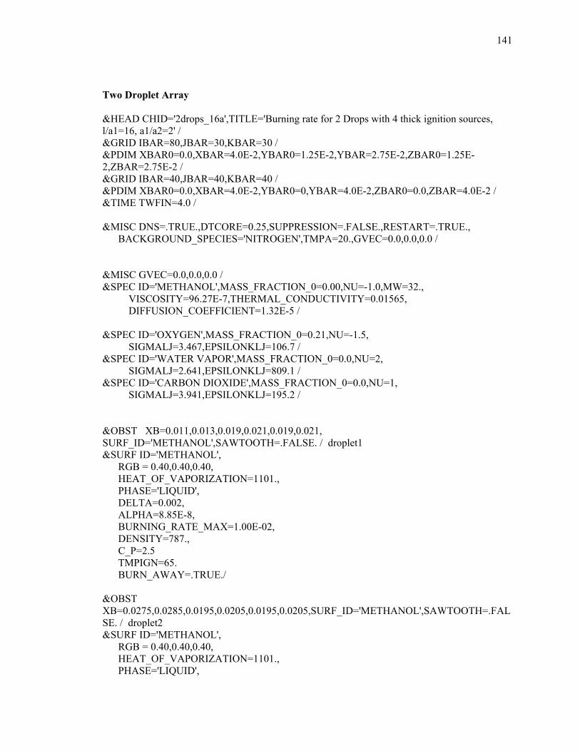
141

Two Droplet Array &HEAD CHID='2drops_16a',TITLE='Burning rate for 2 Drops with 4 thick ignition sources, l/a1=16, a1/a2=2' / &GRID IBAR=80,JBAR=30,KBAR=30 / &PDIM XBAR0=0.0,XBAR=4.0E-2,YBAR0=1.25E-2,YBAR=2.75E-2,ZBAR0=1.25E-2,ZBAR=2.75E-2 / &GRID IBAR=40,JBAR=40,KBAR=40 / &PDIM XBAR0=0.0,XBAR=4.0E-2,YBAR0=0,YBAR=4.0E-2,ZBAR0=0.0,ZBAR=4.0E-2 / &TIME TWFIN=4.0 / &MISC DNS=.TRUE.,DTCORE=0.25,SUPPRESSION=.FALSE.,RESTART=.TRUE., BACKGROUND_SPECIES='NITROGEN',TMPA=20.,GVEC=0.0,0.0,0.0 / &MISC GVEC=0.0,0.0,0.0 / &SPEC ID='METHANOL',MASS_FRACTION_0=0.00,NU=-1.0,MW=32., VISCOSITY=96.27E-7,THERMAL_CONDUCTIVITY=0.01565, DIFFUSION_COEFFICIENT=1.32E-5 / &SPEC ID='OXYGEN',MASS_FRACTION_0=0.21,NU=-1.5, SIGMALJ=3.467,EPSILONKLJ=106.7 / &SPEC ID='WATER VAPOR',MASS_FRACTION_0=0.0,NU=2, SIGMALJ=2.641,EPSILONKLJ=809.1 / &SPEC ID='CARBON DIOXIDE',MASS_FRACTION_0=0.0,NU=1, SIGMALJ=3.941,EPSILONKLJ=195.2 / &OBST XB=0.011,0.013,0.019,0.021,0.019,0.021, SURF_ID='METHANOL',SAWTOOTH=.FALSE. / droplet1 &SURF ID='METHANOL', RGB = 0.40,0.40,0.40, HEAT_OF_VAPORIZATION=1101., PHASE='LIQUID', DELTA=0.002, ALPHA=8.85E-8, BURNING_RATE_MAX=1.00E-02, DENSITY=787., C_P=2.5 TMPIGN=65. BURN_AWAY=.TRUE./ &OBST XB=0.0275,0.0285,0.0195,0.0205,0.0195,0.0205,SURF_ID='METHANOL',SAWTOOTH=.FALSE. / droplet2 &SURF ID='METHANOL', RGB = 0.40,0.40,0.40, HEAT_OF_VAPORIZATION=1101., PHASE='LIQUID',

142

DELTA=0.002, ALPHA=8.85E-8, BURNING_RATE_MAX=1.00E-02, DENSITY=787., C_P=2.5 TMPIGN=65. BURN_AWAY=.TRUE./ &REAC FUEL='METHANOL', FYI='Methyl Alcohol, C H_4 O', MW_FUEL=32. , NU_O2=1.5 , NU_H2O=2., NU_CO2=1., SOOT_YIELD=0.0, RADIATIVE_FRACTION=0.0, BOF=3.2E12,E=125604,XNF=0.25,XNO=1.5,DELTAH=19937./ ! ! ! -- ignition from hot spot ! &SURF ID='IGNITION',TMPWAL=3000.,RAMP_Q='IGN RAMP' / &RAMP ID='IGN RAMP',T=0.0,F=0.0 / &RAMP ID='IGN RAMP',T=0.2,F=1.0 / &RAMP ID='IGN RAMP',T=2.0,F=1.0 / &OBST SURF_ID6='INERT','IGNITION','INERT','INERT','INERT','INERT',XB=0.009,0.010,0.019,0.021,0.019,0.021,T_REMOVE=2.0 / igniter left &OBST SURF_ID6='IGNITION','INERT','INERT','INERT','INERT','INERT', XB=0.0295,0.0305,0.019,0.021,0.019,0.021,T_REMOVE=2.0 / igniter right &OBST SURF_ID6='INERT','INERT','INERT','IGNITION','INERT','INERT',XB=0.019,0.021,0.017,0.018,0.019,0.021,T_REMOVE=2.0 / igniter front &OBST SURF_ID6='INERT','INERT','IGNITION','INERT','INERT','INERT', XB=0.019,0.021,0.022,0.023,0.019,0.021,T_REMOVE=2.0 / igniter back ! ! &VENT CB='XBAR' ,SURF_ID='OPEN' / &VENT CB='XBAR0',SURF_ID='OPEN' / &VENT CB='YBAR' ,SURF_ID='OPEN' / &VENT CB='YBAR0',SURF_ID='OPEN' / &VENT CB='ZBAR' ,SURF_ID='OPEN' / &VENT CB='ZBAR0',SURF_ID='OPEN' / &SLCF PBX=0.0105,QUANTITY='TEMPERATURE',VECTOR=.TRUE. / &SLCF PBX=0.0105,QUANTITY='METHANOL' / &SLCF PBX=0.0105,QUANTITY='DENSITY'/

143

&SLCF PBX=0.0135,QUANTITY='TEMPERATURE',VECTOR=.TRUE./ &SLCF PBX=0.0135,QUANTITY='METHANOL' / &SLCF PBX=0.0135,QUANTITY='DENSITY'/ &SLCF PBX=0.027,QUANTITY='TEMPERATURE',VECTOR=.TRUE. / &SLCF PBX=0.027,QUANTITY='METHANOL'/ &SLCF PBX=0.027,QUANTITY='DENSITY'/ &SLCF PBX=0.029,QUANTITY='TEMPERATURE',VECTOR=.TRUE. / &SLCF PBX=0.029,QUANTITY='METHANOL'/ &SLCF PBX=0.029,QUANTITY='DENSITY'/ &SLCF PBY=0.0185,QUANTITY='TEMPERATURE',VECTOR=.TRUE. / &SLCF PBY=0.0185,QUANTITY='METHANOL' / &SLCF PBY=0.0185,QUANTITY='DENSITY'/ &SLCF PBY=0.0215,QUANTITY='TEMPERATURE',VECTOR=.TRUE./ &SLCF PBY=0.0215,QUANTITY='METHANOL'/ &SLCF PBY=0.0215,QUANTITY='DENSITY'/ &SLCF PBY=0.019,QUANTITY='TEMPERATURE',VECTOR=.TRUE./ &SLCF PBY=0.019,QUANTITY='METHANOL' / &SLCF PBY=0.019,QUANTITY='DENSITY'/ &SLCF PBY=0.021,QUANTITY='TEMPERATURE',VECTOR=.TRUE./ &SLCF PBY=0.021,QUANTITY='METHANOL' / &SLCF PBY=0.021,QUANTITY='DENSITY'/ &SLCF PBZ=0.0185,QUANTITY='TEMPERATURE',VECTOR=.TRUE. / &SLCF PBZ=0.0185,QUANTITY='METHANOL' / &SLCF PBZ=0.0185,QUANTITY='DENSITY'/ &SLCF PBZ=0.0215,QUANTITY='TEMPERATURE' ,VECTOR=.TRUE./ &SLCF PBZ=0.0215,QUANTITY='METHANOL' / &SLCF PBZ=0.0215,QUANTITY='DENSITY'/ &SLCF PBZ=0.019,QUANTITY='TEMPERATURE',VECTOR=.TRUE./ &SLCF PBZ=0.019,QUANTITY='METHANOL' / &SLCF PBZ=0.019,QUANTITY='DENSITY'/ &SLCF PBZ=0.021,QUANTITY='TEMPERATURE',VECTOR=.TRUE./ &SLCF PBZ=0.021,QUANTITY='METHANOL' / &SLCF PBZ=0.021,QUANTITY='DENSITY'/ &TAIL/

144

Three Droplet Asymmetric Array &HEAD CHID='3SF_6a',TITLE='Burning rate for 2 Drops with 4 thick ignition sources, d=2a=2mm, 1.5mm and 1mm' / &GRID IBAR=64,JBAR=64,KBAR=40 / &PDIM XBAR0=1.6E-2,XBAR=4.8E-2,YBAR0=1.6E-2,YBAR=4.8E-2,ZBAR0=2.2E-2,ZBAR=4.2E-2 / &GRID IBAR=44,JBAR=44,KBAR=44 / &PDIM XBAR0=1.0E-2,XBAR=5.4E-2,YBAR0=1.0E-2,YBAR=5.4E-2,ZBAR0=1.0E-2,ZBAR=5.4E-2 / &TIME TWFIN=5. / &MISC DNS=.TRUE.,DTCORE=0.25,SUPPRESSION=.FALSE., BACKGROUND_SPECIES='NITROGEN',TMPA=20.,GVEC=0.0,0.0,0.0 / &SPEC ID='METHANOL',MASS_FRACTION_0=0.00,NU=-1.0,MW=32.042, SIGMALJ=3.626, EPSILONKLJ=481.8 / &SPEC ID='METHANOL1',MASS_FRACTION_0=0.00,NU=-1.0,MW=32., VISCOSITY=96.27E-7,THERMAL_CONDUCTIVITY=0.01565, DIFFUSION_COEFFICIENT=1.32E-5 / &SPEC ID='OXYGEN',MASS_FRACTION_0=0.21,NU=-1.5, SIGMALJ=3.467,EPSILONKLJ=106.7 / &SPEC ID='WATER VAPOR',MASS_FRACTION_0=0.0,NU=2, SIGMALJ=2.641,EPSILONKLJ=809.1 / &SPEC ID='CARBON DIOXIDE',MASS_FRACTION_0=0.0,NU=1, SIGMALJ=3.941,EPSILONKLJ=195.2 / ! !Symmetric configuration, droplets size a1=1mm, a2=0.75mm, a3=0.5mm ! &OBST XB=0.029,0.031,0.03,0.032,0.032,0.034, SURF_ID='METHANOL',SAWTOOTH=.FALSE. / droplet1 &SURF ID='METHANOL', RGB = 0.40,0.40,0.40, HEAT_OF_VAPORIZATION=1101., PHASE='LIQUID', DELTA=0.002, KS=0.20, ALPHA=8.85E-8, BURNING_RATE_MAX=1.00E-02, DENSITY=787., C_P=2.5 TMPIGN=65. BURN_AWAY=.TRUE./

145

&OBST XB=0.032,0.0335,0.037,0.0385,0.032,0.0335, SURF_ID='METHANOL',SAWTOOTH=.FALSE. / droplet2 &SURF ID='METHANOL', RGB = 0.40,0.40,0.40, HEAT_OF_VAPORIZATION=1101., PHASE='LIQUID', DELTA=0.002, KS=0.20, ALPHA=8.85E-8, BURNING_RATE_MAX=1.00E-02, DENSITY=787., C_P=2.5 TMPIGN=65. BURN_AWAY=.TRUE. &OBST XB=0.036,0.037,0.03,0.031,0.032,0.033, SURF_ID='METHANOL',SAWTOOTH=.FALSE. / droplet3 &SURF ID='METHANOL', RGB = 0.40,0.40,0.40, HEAT_OF_VAPORIZATION=1101., PHASE='LIQUID', DELTA=0.002, KS=0.20, ALPHA=8.85E-8, BURNING_RATE_MAX=1.00E-02, DENSITY=787., C_P=2.5 TMPIGN=65. BURN_AWAY=.TRUE./ &REAC FUEL='METHANOL', FYI='Methyl Alcohol, C H_4 O', MW_FUEL=32. , NU_O2=1.5 , NU_H2O=2., NU_CO2=1., EPUMO2=13290., SOOT_YIELD=0.0, RADIATIVE_FRACTION=0.0, BOF=3.2E12,E=125604,XNF=0.25,XNO=1.5,DELTAH=19937./ ! ! ! -- ignition from hot spot ! &SURF ID='IGNITION',TMPWAL=3000.,RAMP_Q='IGN RAMP' / &RAMP ID='IGN RAMP',T=0.0,F=0.0 / &RAMP ID='IGN RAMP',T=0.25,F=1.0 / &RAMP ID='IGN RAMP',T=2.5,F=1.0 /

146

&OBST SURF_ID6='IGNITION','INERT','INERT','INERT','INERT','INERT', XB=0.038,0.039,0.03,0.032,0.032,0.034,T_REMOVE=2.5 / igniter right &OBST SURF_ID6='INERT','IGNITION','INERT','INERT','INERT','INERT', XB=0.027,0.028,0.03,0.032,0.032,0.034,T_REMOVE=2.5 / igniter left &OBST SURF_ID6='INERT','INERT','IGNITION','INERT','INERT','INERT', XB=0.032,0.034,0.040,0.041,0.032,0.034,T_REMOVE=2.5 / igniter back &OBST SURF_ID6='INERT','INERT','INERT','IGNITION','INERT','INERT', XB=0.032,0.034,0.027,0.028,0.032,0.034,T_REMOVE=2.5 / igniter front ! ! &VENT CB='XBAR' ,SURF_ID='OPEN' / &VENT CB='XBAR0',SURF_ID='OPEN' / &VENT CB='YBAR' ,SURF_ID='OPEN' / &VENT CB='YBAR0',SURF_ID='OPEN' / &VENT CB='ZBAR' ,SURF_ID='OPEN' / &VENT CB='ZBAR0',SURF_ID='OPEN' / &SLCF PBX=0.0285,QUANTITY='TEMPERATURE',VECTOR=.TRUE. / &SLCF PBX=0.0285,QUANTITY='METHANOL' / &SLCF PBX=0.0285,QUANTITY='CARBON DIOXIDE' / &SLCF PBX=0.0285,QUANTITY='WATER VAPOR' / &SLCF PBX=0.0285,QUANTITY='DENSITY'/ &SLCF PBX=0.0315,QUANTITY='TEMPERATURE',VECTOR=.TRUE./ &SLCF PBX=0.0315,QUANTITY='METHANOL' / &SLCF PBX=0.0315,QUANTITY='CARBON DIOXIDE' / &SLCF PBX=0.0315,QUANTITY='WATER VAPOR' / &SLCF PBX=0.0315,QUANTITY='DENSITY'/ &SLCF PBX=0.034,QUANTITY='TEMPERATURE',VECTOR=.TRUE. / &SLCF PBX=0.034,QUANTITY='METHANOL'/ &SLCF PBX=0.034,QUANTITY='CARBON DIOXIDE' / &SLCF PBX=0.034,QUANTITY='WATER VAPOR' / &SLCF PBX=0.034,QUANTITY='DENSITY'/ &SLCF PBX=0.0355,QUANTITY='TEMPERATURE',VECTOR=.TRUE. / &SLCF PBX=0.0355,QUANTITY='METHANOL'/ &SLCF PBX=0.0355,QUANTITY='CARBON DIOXIDE' / &SLCF PBX=0.0355,QUANTITY='WATER VAPOR' / &SLCF PBX=0.0355,QUANTITY='DENSITY'/ &SLCF PBX=0.0375,QUANTITY='TEMPERATURE',VECTOR=.TRUE. / &SLCF PBX=0.0375,QUANTITY='METHANOL'/ &SLCF PBX=0.0375,QUANTITY='CARBON DIOXIDE' / &SLCF PBX=0.0375,QUANTITY='WATER VAPOR' / &SLCF PBX=0.0375,QUANTITY='DENSITY'/

147

&SLCF PBY=0.0295,QUANTITY='TEMPERATURE',VECTOR=.TRUE. / &SLCF PBY=0.0295,QUANTITY='METHANOL' / &SLCF PBY=0.0295,QUANTITY='CARBON DIOXIDE' / &SLCF PBY=0.0295,QUANTITY='WATER VAPOR' / &SLCF PBY=0.0295,QUANTITY='DENSITY'/ &SLCF PBY=0.0325,QUANTITY='TEMPERATURE',VECTOR=.TRUE./ &SLCF PBY=0.0325,QUANTITY='METHANOL' / &SLCF PBY=0.0325,QUANTITY='CARBON DIOXIDE' / &SLCF PBY=0.0325,QUANTITY='WATER VAPOR' / &SLCF PBY=0.0325,QUANTITY='DENSITY'/ &SLCF PBY=0.0365,QUANTITY='TEMPERATURE',VECTOR=.TRUE./ &SLCF PBY=0.0365,QUANTITY='METHANOL' / &SLCF PBY=0.0365,QUANTITY='CARBON DIOXIDE' / &SLCF PBY=0.0365,QUANTITY='WATER VAPOR' / &SLCF PBY=0.0365,QUANTITY='DENSITY'/ &SLCF PBY=0.039,QUANTITY='TEMPERATURE',VECTOR=.TRUE./ &SLCF PBY=0.039,QUANTITY='METHANOL' / &SLCF PBY=0.039,QUANTITY='CARBON DIOXIDE' / &SLCF PBY=0.039,QUANTITY='WATER VAPOR' / &SLCF PBY=0.039,QUANTITY='DENSITY'/ &SLCF PBY=0.0315,QUANTITY='TEMPERATURE',VECTOR=.TRUE./ &SLCF PBY=0.0315,QUANTITY='METHANOL' / &SLCF PBY=0.0315,QUANTITY='CARBON DIOXIDE' / &SLCF PBY=0.0315,QUANTITY='WATER VAPOR' / &SLCF PBY=0.0315,QUANTITY='DENSITY'/ &SLCF PBZ=0.0315,QUANTITY='TEMPERATURE',VECTOR=.TRUE. / &SLCF PBZ=0.0315,QUANTITY='METHANOL' / &SLCF PBZ=0.0315,QUANTITY='CARBON DIOXIDE' / &SLCF PBZ=0.0315,QUANTITY='WATER VAPOR' / &SLCF PBZ=0.0315,QUANTITY='DENSITY'/ &SLCF PBZ=0.0345,QUANTITY='TEMPERATURE',VECTOR=.TRUE./ &SLCF PBZ=0.0345,QUANTITY='METHANOL' / &SLCF PBZ=0.0345,QUANTITY='CARBON DIOXIDE' / &SLCF PBZ=0.0345,QUANTITY='WATER VAPOR' / &SLCF PBZ=0.0345,QUANTITY='DENSITY'/ &SLCF PBZ=0.0340,QUANTITY='TEMPERATURE',VECTOR=.TRUE./ &SLCF PBZ=0.0340,QUANTITY='METHANOL' / &SLCF PBZ=0.0340,QUANTITY='CARBON DIOXIDE' / &SLCF PBZ=0.0340,QUANTITY='WATER VAPOR' / &SLCF PBZ=0.0340,QUANTITY='DENSITY'/ &SLCF PBZ=0.0335,QUANTITY='TEMPERATURE',VECTOR=.TRUE./

148

&SLCF PBZ=0.0335,QUANTITY='METHANOL' / &SLCF PBZ=0.0335,QUANTITY='CARBON DIOXIDE' / &SLCF PBZ=0.0335,QUANTITY='WATER VAPOR' / &SLCF PBZ=0.0335,QUANTITY='DENSITY'/ &TAIL/

149

Appendix C: Burning Rate Calculation Samples Table 16 Burning rate calculations for a single 2 mm droplet burning in air X Z V-VELOCITY average velocity DENSITY average density Burning rate m m m/s kg/m3 0.018 0.018 0.002833 0.004146 0.28954 0.282415 2.95E-10

0.0185 0.018 0.003775 0.005464 0.28314 0.27895 3.86E-100.019 0.018 0.004764 0.006745 0.28053 0.278253 4.78E-10

0.0195 0.018 0.005594 0.007597 0.27997 0.278438 5.41E-100.02 0.018 0.005972 0.007673 0.27993 0.278378 5.46E-10

0.0205 0.018 0.005741 0.006975 0.27987 0.278095 4.94E-100.021 0.018 0.005061 0.005853 0.28038 0.27875 4.13E-10

0.0215 0.018 0.004223 0.004685 0.28301 0.282248 3.33E-100.022 0.018 0.00342 0.28951

0.018 0.0185 0.004199 0.005923 0.28065 0.275935 4.14E-10

0.0185 0.0185 0.005777 0.008063 0.27633 0.27413 5.65E-100.019 0.0185 0.007541 0.010235 0.2758 0.274698 7.26E-10

0.0195 0.0185 0.009079 0.011687 0.27671 0.2755 8.36E-100.02 0.0185 0.009745 0.011766 0.27714 0.275423 8.41E-10

0.0205 0.0185 0.009232 0.010482 0.27657 0.274483 7.42E-100.021 0.0185 0.007863 0.008486 0.27556 0.273818 5.94E-10

0.0215 0.0185 0.006265 0.006509 0.27605 0.275603 4.54E-100.022 0.0185 0.004834 0.28042

0.018 0.019 0.005673 0.007596 0.27482 0.271833 5.26E-10

0.0185 0.019 0.008044 0.010582 0.27194 0.270828 7.39E-100.019 0.019 0.01089 0.013694 0.27245 0.271743 9.72E-10

0.0195 0.019 0.013432 0.015776 0.27383 0.272575 1.13E-090.02 0.019 0.014491 0.015862 0.27432 0.27249 1.14E-09

0.0205 0.019 0.013595 0.013962 0.27366 0.271495 9.9E-100.021 0.019 0.011239 0.011043 0.27214 0.27044 7.7E-10

0.0215 0.019 0.008578 0.00823 0.27152 0.271385 5.69E-100.022 0.019 0.006362 0.27442

0.018 0.0195 0.006827 0.008612 0.27143 0.26977 5.94E-10

0.0185 0.0195 0.00984 0.012099 0.26914 0.268978 8.44E-100.019 0.0195 0.013554 0.01576 0.26978 0.269833 1.12E-09

0.0195 0.0195 0.0169 0.018217 0.27091 0.27052 1.31E-090.02 0.0195 0.018282 0.018309 0.27124 0.270435 1.31E-09

150

0.0205 0.0195 0.017078 0.016048 0.27074 0.269575 1.14E-090.021 0.0195 0.013935 0.012593 0.26944 0.26856 8.76E-10

0.0215 0.0195 0.01042 0.009282 0.26866 0.26927 6.38E-100.022 0.0195 0.00756 0.27094

0.018 0.02 0.007272 0.00864 0.27033 0.269755 5.95E-10

0.0185 0.02 0.01051 0.012127 0.26818 0.268958 8.46E-100.019 0.02 0.014493 0.015789 0.26881 0.26981 1.12E-09

0.0195 0.02 0.018092 0.018249 0.26983 0.270495 1.31E-090.02 0.02 0.019592 0.018344 0.2701 0.27041 1.31E-09

0.0205 0.02 0.018282 0.016087 0.26966 0.269553 1.14E-090.021 0.02 0.014898 0.012634 0.26846 0.268543 8.79E-10

0.0215 0.02 0.011119 0.009322 0.26768 0.269258 6.41E-100.022 0.02 0.008028 0.2698

0.018 0.0205 0.006881 0.007676 0.27141 0.271798 5.31E-10

0.0185 0.0205 0.009896 0.010663 0.2691 0.270775 7.45E-100.019 0.0205 0.013611 0.013781 0.26974 0.27168 9.78E-10

0.0195 0.0205 0.016961 0.015873 0.27086 0.272503 1.14E-090.02 0.0205 0.01835 0.015969 0.27119 0.27242 1.14E-09

0.0205 0.0205 0.017152 0.014079 0.27069 0.271435 9.98E-100.021 0.0205 0.014017 0.011165 0.2694 0.27039 7.78E-10

0.0215 0.0205 0.010503 0.008349 0.26863 0.271353 5.77E-100.022 0.0205 0.007638 0.27092

0.018 0.021 0.005779 0.006045 0.2748 0.275905 4.22E-10

0.0185 0.021 0.008148 0.00818 0.27188 0.27407 5.73E-100.019 0.021 0.010999 0.010371 0.27238 0.274613 7.35E-10

0.0195 0.021 0.013554 0.011847 0.27374 0.275398 8.47E-100.02 0.021 0.014628 0.011941 0.27422 0.275323 8.53E-10

0.0205 0.021 0.013746 0.010667 0.27358 0.274398 7.55E-100.021 0.021 0.011399 0.008677 0.27207 0.273753 6.07E-10

0.0215 0.021 0.00874 0.006701 0.27146 0.275573 4.68E-100.022 0.021 0.006516 0.2744

0.018 0.0215 0.004352 0.00431 0.28065 0.282425 3.07E-10

0.0185 0.0215 0.0059 0.005619 0.27629 0.278918 3.97E-100.019 0.0215 0.007674 0.006929 0.27573 0.278178 4.91E-10

0.0195 0.0215 0.009259 0.007818 0.2766 0.27834 5.57E-100.02 0.0215 0.009949 0.007907 0.27703 0.278283 5.63E-10

0.0205 0.0215 0.009442 0.007215 0.27646 0.27802 5.11E-100.021 0.0215 0.00808 0.006103 0.27548 0.278713 4.31E-10

0.0215 0.0215 0.006491 0.00494 0.276 0.282268 3.51E-10

151

0.022 0.0215 0.005058 0.28043 0.018 0.022 0.003037 0.2896

0.0185 0.022 0.003951 0.28316 0.019 0.022 0.004952 0.28049

0.0195 0.022 0.005833 0.27989 0.02 0.022 0.006232 0.27984

0.0205 0.022 0.006006 0.2798 0.021 0.022 0.005334 0.28034

0.0215 0.022 0.004506 0.28303 0.022 0.022 0.003704 0.28961

2.82E-07

152

Appendix D: Experimental Set-Up

Table 17 Mechanical Equipment List

System Component Manufacturer Model Status

Piezoelectric transducers Channel Industries C-0509-620 Operational at NASA GRC

Front/rear transmitter blocks Drexel University Custom Operational at NASA GRC

Acoustic Horn SonicEase Custom Operational at NASA GRC

Acoustic Reflector Drexel University Custom On hand at NASA GRC

Reflector Traverse Haydon Switch and Instrument, Inc. (HSI) 20542-12-035 On hand at NASA GRC

Stepper Motor Controller Haydon Switch and Instrument, Inc. L/R 39105 On hand at NASA GRC

Signal Amplifier Optimus XL-200 Operational at NASA GRC

Frequency Generator Agilent 33120A Operational at NASA GRC

Step-up Transformer Circuit Drexel University Custom Breadboard operational at NASA GRC

Control Circuit NASA GRC Custon Breadboard operational at NASA GRC

Syringe Pump NASA GRC Custom Use as-is from HPDCE

Needle positioner Haydon Switch and Instrument, Inc. 20842-12 On-hand at NASA GRC; bracket

must be designed.

Stepper Motor Controller Haydon Switch and Instrument, Inc. L/R 39105 On-hand at NASA GRC

High Voltage Power Supply American High Voltage EC Series Use circuit as-is from HPDCE

Ignitor Igniter Assembly NASA GRC Custom Hot wire, igniter movement, and elevator in testing at NASA GRC

LED and control NASA GRC Custom Use as-is from HPDCE

Camera 1 mount (side view) NASA GRC Custom Need to design and fab mount

Camera 2 mount (top down) NASA GRC Custom Need to design and fab mount

Lens supports NASA GRC Custom Need to design and fab

Power Distribution Module NASA GRC Custom to be obtained

TT8-DDACS NASA GRC Custom to be obtained

Relay box NASA GRC Custom Use as-is from HPDCE

DC-AC Inverter Sinergex PureWatts 300 On-hand at NASA GRC

Purge bottle Swagelok TBD must be sized and ordered

Enclosure NASA GRC Custom 8020 structure, top and two sides Lexan, other sides aluminum

General

Acoustic Levitator

Signal Generation

Droplet Insertion

Diagnostics

153

Table 18 Experiment Controls Timeline Time (sec) Action Control Requirement

-90 Initiate acoustic field Turn on waveform generator (Manually)

-70 Turn on LED Close Relay 4

-60 Turn on cameras digital output from D/O - 3: (ch. 15 and 18)

-60 Turn on VCR Manual Control

-50 Move droplet

insertion needle into

the acoustic field

Activate Needle Control Motor FWD (digital output from

D/O - 3 (ch. 16))

-40 Turn on HV power

supply

Close Relay 7

-40 Disperse liquid

droplet to end of

needle

Move Fuel Supply Motor FWD (Close Relay 3 FWD;

open upon moving specified amount)

-20 Jog reflector to

release droplets

digital output from D/O - 3 (ch. 17)

-15 Turn off HV power

supply

Open Relay 7

-15 Withdraw droplet

insertion needle

Activate Needle Control Motor REV (digital output from

D/O - 3 (ch. 16))

-10 Move igniter elevator

to HIGH position

Move Igniter Elevator Motor FWD (Relay 5 FWD)

154

-5 Move igniter arm into

position

Move Igniter Arm Motor FWD (Relay 6 FWD)

-5 Initiate data logging Thermocouples

-2 Turn on hot wire Activate Relay 8

0 Initiate acoustic field

ramp profile

Initiate ramp profile on the drop indication (digital output

from D/O - 4 (ch. 21&22))

0.5 Turn off hot wire De-active Relay 8

0.5 Retract igniter arm Move Igniter Arm Motor REV (Relay 6 REV)

0.5 Move igniter elevator

to LOW position

Move Igniter Elevator Motor REV (Relay 5 REV)

2.2 End of Drop

2.5 Turn off cameras digital output from D/O - 3: (ch. 15 & 18)

3 Terminate data

logging

3 Turn off LED,

acoustic field ramp,

waveform generator,

etc.

Remove power from all relays

5 Turn off VCR Manual Control

155

Appendix E: Nomenclature

a fuel droplet radius

ai, aj fuel droplet radius for the “i” or “j” droplet in the array

b* non-dimensional half inter-droplet spacing

B pre-exponential factor for Arrhenius reaction; Spalding transfer number

cp constant pressure specific heat

dq air-fuel mixture diameter

D diffusion coefficient

D* characteristic fire diameter

E activation energy

f external force vector (excluding gravity)

g acceleration of gravity

H total pressure divided by the density

h enthalpy; heat transfer coefficient

hi enthalpy of ith species

h0i heat of formation of ith species

hfg enthalpy of formation

I radiation intensity

Ib radiation blackbody intensity

Ja Jacob number, ( ) fgsatp hTTc /−∞

k thermal conductivity; suppression decay factor

156

l distance between droplets in an array, measured from droplet’s center

l/a non-dimensional spacing between droplets in an array, as the ration of distance between droplets and droplet radius

M molecular weight of the gas mixture

Mi molecular weight of ith gas species

m& mass evaporation rate of a droplet in array

isom& mass evaporation rate of an isolated droplet

fm ′′& fuel mass flux

im ′′′& mass production rate of ith species per unit volume

Om ′′& oxygen consumption rate per unit area

N number of droplets in a cluster (array)

Nu Nusselt number

Pr Prandtl number

p pressure

p0 background pressure

p~ pressure perturbation

qr radiative heat flux vector

q& ′′′ heat release rate per unit volume

rq ′′& radiative flux to a solid surface

cq ′′& convective flux to a solid surface

Q& total heat release rate

157

*Q characteristic fire size

rr radial position vector

ℜ universal gas constant

Re Reynolds number

s unit vector in direction of radiation intensity

Sc Schmidt number

Sh Sherwood number

T temperature

∞T ambient temperature

wT droplet surface temperature

t time

u = (u,v,w) velocity vector

x = (x,y, z) position vector

Xi volume fraction of ith species

Yi mass fraction of ith species

∞OY mass fraction of oxygen in the ambient

IFY mass fraction of fuel in the fuel stream

H∆ heat of combustion

OH∆ energy released per unit mass oxygen consumed

ε emission coefficient

δ wall thickness

η correction factor (similarity parameter)

158

λ wavelength

kε Lennard-Jones potential parameter ([K])

κ absorption coefficient

µ dynamic viscosity

iν stoichiometric coefficient, species i

Φ dissipation function; equivalence ration

DΩ diffusion collision integral

ρ gas-phase density

τ viscous stress tensor

σ Stefan-Boltzmann constant, Lennard-Jones coefficient ([Å])

lmσ Lennard-Jones coefficient ([Å])

sσ scattering coefficient

159

Curriculum Vitae Irina N. Ciobanescu Husanu

EDUCATION

Drexel University, Philadelphia, PA Ph.D. in Mechanical Engineering 2005 Dissertation: “Droplet Interactions during Combustion of Unsupported Droplet Clusters in Microgravity: Numerical Study of Droplet Interactions at Low Reynolds Number”

Polytechnic University of Bucharest, Romania B.S. /M.S. in Aeronautical Engineering 1990

Thesis: “Calculus and Design of a Turboprop Aircraft Engine. The Influence of the Profiling Law on Engine Performances for Rotor Blades of the Compressor”

TEACHING AND RESEARCH EXPERIENCE Delaware County Community College, Media, PA Adjunct Instructor – MATH 100 “Intermediate Algebra” 2006 Developed syllabus and overall course structure, and administered all grades. Developed teaching strategies for individual instruction.

Drexel University, Philadelphia, PA Teaching Assistant –in “Thermodynamics”, “Thermodynamics Analysis”, “Heat Transfer”, “Fluid Mechanics”, “Internal Combustion Engines”, “HVAC Controls”, “Dynamics”, “Aerospace Structures”

2003-2005

Collaborated on curriculum, projects and exam development, held lectures and all recitation classes, met with students on regular basis, and graded all written work, including final exam papers.

Research Assistant (Research Fellow) 2000-2004

Study of Ice Accretion using LEWICE Code - Computational Evaluation of Icing Scaling Methods and development of Ice Accretion Model Droplet Interactions at Low Reynolds Numbers - Analytical investigation of droplet interactions during vaporization and combustion of asymmetric droplet clusters in microgravity (spatial asymmetric geometry of the array as well as different droplets sizes for a given fuel)

RELATED EXPERIENCE

Ministry of Foreign Affairs, Romania Diplomat 1997-2000

Ministry of Research and Development, Romania Senior Governmental Expert 1994- 1997

Company for Turbo-machinery and Engineering, Bucharest, Romania Researcher 1990-1997

University “Titu Maiorescu” Bucharest, Romania

Part Time Mathematics Instructor 1992-2000

PUBLICATIONS AND PAPERS

“Droplet Interactions during Combustion of Unsupported Droplet Clusters in Microgravity: Numerical Study of Droplet Interactions at Low Reynolds Number”, Bell & Howell, 2006 “Combustion of Unsupported Droplet Clusters in Microgravity”, Poster Session of 30th International Symposium of Combustion Institute, 2004 “Combustion of Unsupported Clusters of Droplets in Microgravity”, G.A. Ruff, S. Liu, I. Ciobanescu, KAIST Workshop, Drexel University, 2003

160

“Droplet Vaporization in a Levitating Acoustic Field”, G.A. Ruff, S. Liu, I. Ciobanescu, Proceeding of 7th International Workshop on Microgravity Combustion and Chemically Reacting Systems, 2003 “Teleworking, Concept and Definitions”, A. Toia, S. Dragomirescu, I. Ciobanescu, G. Macri, 1996 “Tele-Health”, A. Toia, I. Ciobanescu, 1997 “Social and Economic Impact of Teleworking”, A. Toia, S. Dragomirescu, I. Ciobanescu, G. Macri, 1997

LANGUAGES English – speak fluently and read/write with high proficiency

Romanian – native language French – speak fluently and read/write with high proficiency

MEMBERSHIPS Member of Student Chapter of Combustion Institute HISTORY Born in Bucharest, Romania in 1966

Married to Cristian Husanu and has three children: Catalin, Diana and Ana