drop generation using cross-flow in rigid body rotation
TRANSCRIPT

University of Nebraska - LincolnDigitalCommons@University of Nebraska - LincolnMechanical (and Materials) Engineering --Dissertations, Theses, and Student Research
Mechanical & Materials Engineering, Departmentof
Winter 11-30-2018
Drop Generation Using Cross-Flow in Rigid BodyRotationHaipeng ZhangUniversity of Nebraska - Lincoln, [email protected]
Follow this and additional works at: http://digitalcommons.unl.edu/mechengdiss
Part of the Materials Science and Engineering Commons, and the Mechanical EngineeringCommons
This Article is brought to you for free and open access by the Mechanical & Materials Engineering, Department of at DigitalCommons@University ofNebraska - Lincoln. It has been accepted for inclusion in Mechanical (and Materials) Engineering -- Dissertations, Theses, and Student Research by anauthorized administrator of DigitalCommons@University of Nebraska - Lincoln.
Zhang, Haipeng, "Drop Generation Using Cross-Flow in Rigid Body Rotation" (2018). Mechanical (and Materials) Engineering --Dissertations, Theses, and Student Research. 142.http://digitalcommons.unl.edu/mechengdiss/142

Drop Generation Using Cross-Flow in Rigid Body Rotation
By
Haipeng Zhang
A THESIS
Presented to the Faculty of
The Graduate College at the University of Nebraska
In Partial Fulfillment of Requirements
For the Degree of Master of Science
Major: Mechanical Engineering and Applied Mechanics
Under the supervision of Professor Sangjin Ryu
Lincoln, Nebraska
November, 2018

ii
Drop Generation Using Cross-Flow
in Rigid Body Rotation
Haipeng Zhang, M. S.
University of Nebraska, 2018
Advisor: Sangjin Ryu
Inspired by crossflow membrane droplet generation and microfluidic droplet
generation, I propose an easy method to generate monodisperse drops using cross-flow
caused by rigid body rotation. In this approach, a dispersed phase (DP) liquid was
injected through a stationary vertical needle into an immiscible continuous phase (CP)
liquid which was in rigid body rotation. A DP drop growing at the end of the needle
experienced fluid dynamic forces from the horizontal CP flow, and it was detached from
the needle when it had grown to a certain size. This study investigated the relationship
between the resultant size of drops and the controllable experimental factors including
the flow velocity of the CP at the needle end and the flow rate of the DP through the
needle.

iii
ACKNOWLEDGEMENTS
Firstly, I would like to thank the harsh life. The difficulty of life pushed me forward.
I would like to thank my advisor, Dr. Sangjin Ryu, for the help of my research and
the advice of daily life. I would like to thank Dr. Jae Sung Park and Dr. Seunghee Kim
for helping me through my research career and being my thesis committee.
I would like to thank Dr. Howard Stone in Princeton University for discussion. I
would like to thank Dr. Timothy Wei for the macro lens of high-speed camera. I also
would like to thank Ali Mazaltarim in the Department of Chemistry for the help of
surface tension coefficient measurement.
I would like to thank my lab mates, Donghee Lee, Jacob Gottberg, Tomer Palmon,
Dilziba Qizghin, and Stephanie Vavra, for their help of my research and support in the
laboratory. I would like to thank the lab members in Park Research Group, Ethan Davis,
Siamak Mirfendereski, and Thomas Hafner, for the discussions of my research. I also
would like to thank Luz Sotelo for helping me to improve my presentation.
I would like to thank Terri Eastin in the office of graduate studies, Kathie Hiatt,
Mary Ramsier, Cherie Crist, Heidi Krier, and other staffs in the department office, for
helping me to get the master’s degree. I would like to thank Alan Wilkins in ISSO for
the supporting information of graduate studies. I also would like to thank the Lincoln
Literacy, Clay Farris Naff, Rik Minnick, and other staffs’ help about the language and
our lives in the United States.
I would like to thank the faculties of the Kitami Institute of Technology in Japan,

iv
Hiroshi Sakamoto, Hiroyuki Haniu, and Kazunori Takai, for leading me into the
scientific research career.
I would also like to thank the members of the pump department of Kubota
Corporation in Japan, Hirohiko Yamada, Teruo Miura, Makoto Sano, Hiroyuki Ishimi,
and Kazuo Nishimura. I couldn’t become a graduate student without their support.
Finally, I would like to thank my family. My parents Jianfeng Zhang and Zhiquan
Duan, my parents-in-law Litan He and Dongmei He are supporting me continuously. I
would like to thank my wife, Ling He. She is always staying with me to against hard
time.
v
Table of Contents
ACKNOWLEDGMENTS……………………………………...…………………….iii
List of Figures…………………………………………………………..…………….vii
List of Tables…………………………………………………………………………...x
Chapter 1 Introduction………………………………………….………………...……1
1.1 Crossflow-based Drop Generation Methods……………………………..……2
1.1.1 Membrane Emulsification Method……………………………………..3
1.1.2 Crossflow-based Microfluidic Drop Generators………………………..4
1.2 Pinch-off Principles of Drop Generation Process in Crossflow……………….6
1.2.1 The Squeezing Mode in Crossflow……………………………………..7
1.2.2 The Dripping Mode in Crossflow…………………………………….....9
1.2.3 The Jetting Mode in Crossflow………………………………………..10
1.3 The Models for Drop Sizes Prediction in Crossflow…………………………11
1.3.1 The Dimensionless Parameter-based Map…………………………….12
1.3.2 The Nondimensional Number-based Map……………………………..13
1.3.3 The Torque Balance Equation…………………………………………17
1.4 Rigid Body Motion Driven Crossflow-based Drop Generation…………….18
1.4.1 Motivation…………………………………………………………….18
1.4.2 Working Principle……………………………………………………..19
Chapter 2 Methods and Materials…………………………………………………….22
2.1 Materials……………………………………………………………………..22
2.2 Experimental Setup…………………………………………………………..26

vi
2.3 Experimental Procedures…………………………………………………….30
2.4 Image Correction…………………………………………………………….32
2.5 Image Processing of Drops…………………………………………………..36
Chapter 3 Results……………………………………………………………………..39
3.1 Experimental Images and Drop Pinch-off Modes of the Drops………………39
3.2 Drop Diameter Distribution………………………………………………….48
3.3 Dimensionless Phase Diagram of the Drop Generation……………………..52
3.4 The Different Pinch-off Zones in the Nondimensional Analysis Phase
Diagram………………………………………………………………………………54
3.5 The Application of the Nondimensional Analysis Phase Diagram……….….56
Chapter 4 Discussion…………………………………………………………………58
4.1 Absence of the Squeezing Mode……………………………………………..58
4.2 Controlling Drop Diameter…………………………………………………..58
4.3 Nondimensional Numbers in the Drop Generation Processes……………….60
4.4 The Studies of Force Balanced Equation…………………………………….66
Chapter 5 Conclusions………………………………………………………………..71
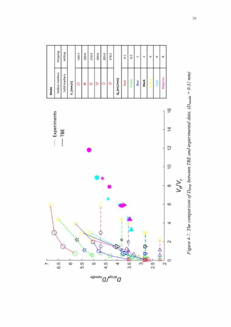
Appendix A. The Measurement Results of Drop Sizes……………………………….73
Appendix B. The Size Distributions of Generated Drops…………………………….77
Appendix C. The Calculation of Dimensionless Parameters………………………….94
Appendix D. The Calculation of Nondimensional Numbers…………………………98
Appendix E. The Calculation of Torque Balance Equation……………………….…106
References…………………………………………………………………………..110

vii
List of Figures
Figure 1-1. The working process of drop-based cell encapsulation method. ……..……1
Figure 1-2. The schematic figure of the principle of the crossflow-based drop
generation……………………………………………………………………………...3
Figure 1-3. The schematic figure of the membrane emulsification method……………4
Figure 1-4. The schematic figure of the T-junction microfluidic drop generator………5
Figure 1-5. The schematic figure of other microfluidic drop generators……………….6
Figure 1-6. The images of the squeezing mode, the dripping mode, and the jetting mode-
based drop generation in the T-junction device………………………………………..7
Figure 1-7. The formation process of the drops in the squeezing mode……………….8
Figure 1-8. The formation process of the drops in the dripping mode………………..10
Figure 1-9. The formation process of the drops in the jetting mode…………………..11
Figure 1-10. An example of the dimensionless parameter-based map for drop
generation…………………………………………………………………………….13
Figure 1-11. An example of the nondimensional number-based map for drop
generation…………………………………………………………………………….15
Figure 1-12. An example of Ca-We-Oh-based map for pinch-off modes…………….16
Figure 1-13. The experimental setup for the Ca-We-Oh-based map example…….….16
Figure 1-14. An example of We-Ca/Oh-based map for pinch-off modes……….…….17
Figure 1-15. The experimental setup for the We-Ca/Oh-based map example…….….17
Figure 1-16. The schematic of TBE model in drop generation……………………….18
Figure 1-17. The principle of the rigid body motion driven drops generation system…20

viii
Figure 1-18. The schematic figure of the rigid body motion driven drops generation
system……………………………………………………………………...…………20
Figure 2-1. The viscosity measurement results of the rheometer…………………….24
Figure 2-2. The interfacial surface tension coefficient measurement results of the
goniometer……………………………………………………………………………25
Figure 2-3. Experiment setup of drop generation…………………………………….26
Figure 2-4. The grid plate attached on the needle holder for image correction……….31
Figure 2-5. A reference image of the grid plate in the continuous phase……………..31
Figure 2-6. A raw image of drop generation processes (R = 80 mm, Ω = 4.7 rad/s, and
Qd = 0.5 mL/min.)…………………………………………………………………….33
Figure 2-7. The x and y coordinates measurements of the intersection points from the
reference image……………………………………………………………………….34
Figure 2-8. A cropped raw image of drop generation processes………………………35
Figure 2-9. An adjusted image of drop generation processes…………………………35
Figure 2-10. The measurement processes of drops in the ADM………………………37
Figure 3-1. The drop generation process of Vc = 210.42 mm/s, and Vd = 543.67 mm/s..40
Figure 3-2. The drop generation process of Vc = 210.42 mm/s, and Vd = 2174.68
mm/s………………………………………………………………………………….40
Figure 3-3. Drop size distribtion of Vc = 140.3 mm/s or 189.0 mm/s, Vd = 543.7 mm/s,
Dneedle = 0.14 mm……………………………………………………………………..49
Figure 3-4. The histograms of Vc = 140.28 mm/s or 189.04 mm/s, Vd = 2174.68 mm/s,
Dneedle = 0.14 mm……………………………………………………………………..50

ix
Figure 3-5. The map of the nondimensional analysis phase diagram…………………53
Figure 3-6. The zones of pinch-off modes in the nondimensional analysis phase
diagram……………………………………………………………………………….55
Figure 3-7. The applications of the nondimensional analysis phase diagram………...57
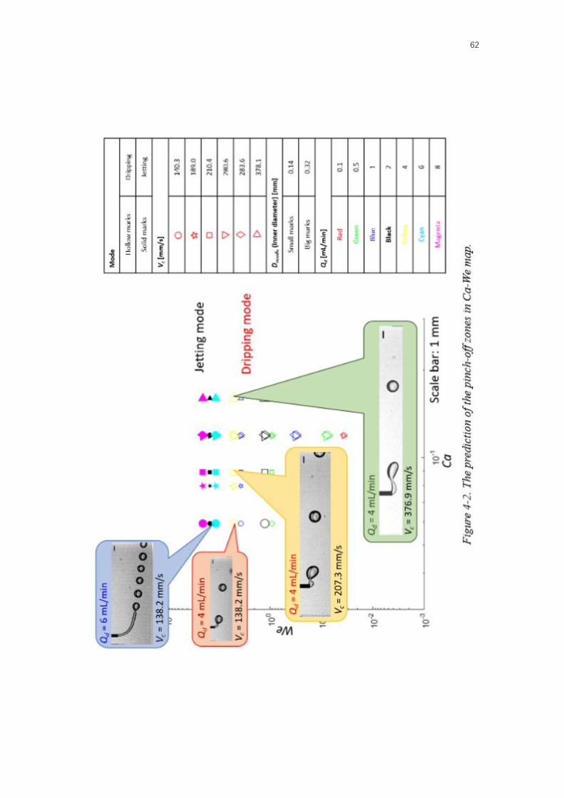
Figure 4-1. The nondimensional number-based map (Ca-We)………………………..61
Figure 4-2. The prediction of the pinch-off zones in Ca-We map……………………..62
Figure 4-3. The nondimensional number-based map (Ca/OhCP-We)……………..…..64
Figure 4-4. The comparison of nondimensional number-based map (Ca/Oh-We)……65
Figure 4-5. The schematic figure of TBE in this study……………………………….67
Figure 4-6. The comparison of Ddrop between TBE and experimental data. (Dneedle =
0.14 mm)……………………………………………………………………………...69
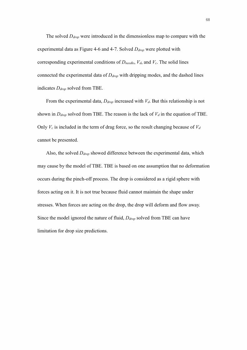
Figure 4-7. The comparison of Ddrop between TBE and experimental data. (Dneedle =
0.32 mm)…………………………………………………………………………..….70
x
List of Tables
Table 2-1 The measurement results of mass (unit: g)………………………………….23
Table 2-2. The measured properties of the CP and the DP……………………………25
Table 2-3. The experimental conditions applied for the drop generation processes.…28
Table 2-4. Vc values calculated from the experimental conditions…………………...29
Table 2-5. Vd values calculated from the experimental conditions……………………29
Table 2-6. The calculation results of tilted angles and elongated aspect ratios……….35
Table 2-7. Pixel size for different experimental conditions…………………………...36
Table 3-1. Drop generations with Dneedle = 0.14 mm (scale bar = 1 mm)…………….41
Table 3-2. Drop generations with Dneedle = 0.32 mm (scale bar = 1 mm)…………….44
Table 3-3. The comparison of drop monodispersity between different methods……..51
Table A-1. The drop diameters with various experimental conditions………………..73
Table B-1. The histograms of experiments with Dneedle = 0.14 mm…………………..77
Table B-2. The histograms of experiments with Dneedle = 0.32 mm……………………83
Table B-3. The calculation results of CV……………………………………………..90
Table C-1. The parameters of the nondimensional analysis………………………….94
Table D-1. The calculations of the nondimensional numbers (Ca and We)……………98
Table D-2. The calculations of the nondimensional numbers (OhCP and Ca/OhCP)…102
Table E-1. The calculations of Ddrop using TBE…………………….……………….106

1
Chapter 1 Introduction
A drop is a deformable liquid sphere with limited volume and high surface-area-
to-volume ratio. Drops are widely used in multiple areas for various purposes, including
industrial applications and scientific researches [1, 2]. Drops can be used for changing
the physical properties of emulsions. For example, the viscosity of emulsion can be
changed by varying shear rates on drops because of their deformability. A similar
application was developed for changing the elasticity of emulsion based on the surface
tension difference of drops [3, 4]. Additionally, drops are used to control chemical or
biochemical reactions as microreactors. There are several advantages of the drop-based
microreactor: less reagent consumption because of the limited volume of drops, and
faster reaction processes because of the high surface-area-to-volume ratio [5].
Furthermore, drops are used in complicated experimental systems for cells minor
control. Figure 1-1 is an example of the drop-based cell encapsulation method in a drop
generation system. The drops containing cells are delivered to the downstream direction
for further manipulations [6].
Figure 1-1 The working process of drop-based cell encapsulation method [7, 8].
(Scale bar: 100 μm)

2
Because of the various applications of drops in chemistry, electronics, cosmetics,
foods, and pharmaceuticals, the requirements of monodispersed drop generators have
been increasing [9-11]. A well-designed drop generator must be able to generate drops
continuously with predictable sizes. The focus of this study is to develop a reliable drop
generator for easier and cheaper production of monodispersed drops in the laboratory.
1.1 Crossflow-based Drop Generation Methods
Many different drop generation methods were developed in the past years. A well-
known subgroup is the crossflow-based drop generation methods [12-18]. Figure 1-2
shows the principle of the crossflow-based drop generation. Two immiscible liquid
phases, the continuous phase (CP) and the dispersed phase (DP), are injected into a
device with a certain designed channel structure [19]. The structure can lead the stream
of the CP and DP meet with each other. The interface between these two phases occurs
where the CP and DP meet [2, 20]. The interface deforms while the CP and DP are
injected. Eventually, a certain amount of the DP is pinched-off from the stream of DP.
The separated portion of the DP becomes spherical shape automatically because of the
surface tension. Afterwards, the drops are delivered by the CP in the direction of the CP
flow. By injecting the CP and DP continuously, the drop generation process can be
continued [4]. Based on the basic principle of the crossflow, different crossflow-based
drop generators have been developed.

3
Figure 1-2 Schematic figure of the principle of the crossflow-based drop generation
[13].
1.1.1 Membrane Emulsification Method
The membrane emulsification method is developed based on the crossflow [13, 15].
Because of the high frequency of drop generations, the method has drawn attentions
and is widely used in industrial areas. Figure 1-3 is a schematic figure of the membrane
emulsification method. The DP is injected through multiple pores or capillary tubes of
a flat membrane at a volume flow rate Qd. The CP is flowed with volume flow rate Qc
in the direction parallel to the membrane surface. Depending on the Qd, a part of the DP
stream passing through the pores become spherical at the surface of the membrane.
After the spherical DPs grow to certain sizes, the shear force caused by CP acting along
the membrane surface can seperate the spherical DPs from the DP streams. Due to the
high numbers of the pores in the membrane, huge amount drops are pinched-off when
the CP swept the surface of the membrane.
For different requirements, minor changes such as the shape of the membrane are

4
considered for the membrane emulsification method [2]. The shape of the membrane
does not have to be flat. Cylindrical tube-shaped membranes are also used for easier
collection of drops. Different geometry designs of the membrane structures and the
experimental conditions of the working fluids are used for various purposed
applications [13, 15, 21-31].
Figure 1-3. The schematic figure of the membrane emulsification method [2].
1.1.2 Crossflow-based Microfluidic Drop Generators
The crossflow-based microfluidic drop generators are another series of drop
generation method. The CP and DP are injected through tubing into a microfluidic
device with micro-scales channels inside. The micro channels define the flow directions
of CP and DP, the positions where CP meet with DP, and an angle θ (0° < θ ≤ 180°)
between the flow directions of the two immiscible phases. The selection of the materials
for making microfluidic devices is flexible. The polydimethylsiloxane (PDMS), glass,
and 3D printed materials are used [2, 32]. Because of the micro-scaled device, the
crossflow-based microfluidic drop generators are well used in laboratory for drop
generation with sensitive controlling.

5
Figure 1-4 is a well-known design of the microfluidic PDMS drop generation
devices named as the T-junction device [33, 34] . The T-junction device is a simple
design which is good for microfluidic research. 3 holes on the device are used as the
inlet of the CP, the inlet of the DP, and the outlet of the drops, respectively. The volume
flow rate of CP and DP are applied as Qc and Qd, respectively. The width of the channels
for the inlet of the continuous phase, the inlet of the dispersed phase, and the outlet are
indicated as wc, wd, and wo, respectively. The flow directions of the CP and DP are
following the direction of the micro channels. At the junction, CP meet with DP at 90°,
and then break a drop from the stream of DP. By using the T-junction microfluidic
device, the drops of DP are generated continuously to the outlet.
Figure 1-4. The schematic figure of the T-junction microfluidic drop generator [2].
The similar idea but different micro channel designs are also used. Figure 1-5 a-d
are other crossflow-based microfluidic device designs. Figure 1-5a is the T-junction
with θ other than 90° (0° < θ ≤ 180°). Figure 1-5b is named as Head-on geometry device
with θ = 180°. Figure 1-5c is the Y-shaped junction. Figure 1-5d is the double T-junction
because of the combined shape of two T-junctions [35]. For specific requirements or
working conditions, some accessories, such as a piezo electric bending disc, can be used
in the microfluidic system for promoting the formation processes of drops [11].

6
Different novelties are included in these designs, but the basic ideas of drop generation
processes are the same as in the T-junction device.
Figure 1-5. The schematic figure of other microfluidic drop generators [2].
1.2 Pinch-off Principles of Drop Generation Process in Crossflow
In order to satisfy the requirements of different purposes, the sizes of drops
generated from the devices should be predictable. Since the experimental data revealed
that the range of drop sizes are various for different pinch-off modes, the studies of drop
size predictions are started from understanding the principles of drop pinch-off modes
[2, 21].
Three pinch-off modes, the squeezing mode, the dripping mode, and the jetting
mode, are identified in the various crossflow-based drop generators [2, 21, 36]. For
demonstration, the pinch-off processes of drops in the T-junction microfluidic PDMS
device are studied. Figure 1-6 a-c shows the images of these three pinch-off modes in
the T-junction device. Each pinch-off mode has the corresponding experimental
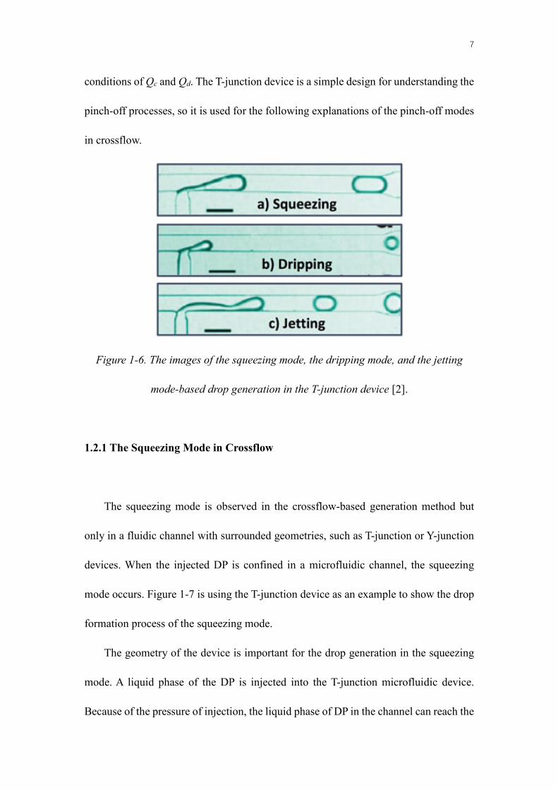
7
conditions of Qc and Qd. The T-junction device is a simple design for understanding the
pinch-off processes, so it is used for the following explanations of the pinch-off modes
in crossflow.
Figure 1-6. The images of the squeezing mode, the dripping mode, and the jetting
mode-based drop generation in the T-junction device [2].
1.2.1 The Squeezing Mode in Crossflow
The squeezing mode is observed in the crossflow-based generation method but
only in a fluidic channel with surrounded geometries, such as T-junction or Y-junction
devices. When the injected DP is confined in a microfluidic channel, the squeezing
mode occurs. Figure 1-7 is using the T-junction device as an example to show the drop
formation process of the squeezing mode.
The geometry of the device is important for the drop generation in the squeezing
mode. A liquid phase of the DP is injected into the T-junction microfluidic device.
Because of the pressure of injection, the liquid phase of DP in the channel can reach the

8
wall of the channel and grow continuously in the channel toward the outlet after passing
the junction. Eventually, the channel is clogged by the liquid phase of DP. The flow
direction of CP is the same as the liquid phase, so CP is stopped in the channel. A huge
pressure difference between the both sides of the DP phase occurs because of the
growing DP phase and the injection of CP. Once the pressure difference between the
both sides of DP clog is high enough, the connection of the injected DP and the DP clog
in the channel will be broken. The elongated-shaped clog of the DP is pushed away by
the CP flow toward the outlet of the channel. After leaving the surrounded boundaries
of the channel, the clog of DP can become spherical automatically because of the
surface tension [36].
Flow direction of CP →
Figure 1-7. The formation process of the drops in the squeezing mode [37].
Two characteristics of the drops in the squeezing mode can be found. The first one
is the larger sizes of the drops. The total volume of the drops in the squeezing mode can
be approximately calculated as the product of the cross-section area of the channel and
the length of the clog. The second one is the requirement of the surrounded geometry.

9
Without a channel confining the DP, the pressure difference between the both sides of
the DP cannot support the squeezing mode. For instance, there is no drop in the
squeezing mode observed in the membrane emulsification method. Because the DP in
the membrane emulsification method is not confined after passing through the pores,
the pressure difference among a spherical-shaped DP on the surface of the membrane
is negligible. Without the high enough pressure difference, the squeezing mode does
not occur [36, 37].
1.2.2 The Dripping Mode in Crossflow
The formation process of the dripping mode is shown in Figure 1-8. The
detachment of the dripping mode occurs at the junction. The liquid phase of DP can
pass over the subchannel when the DP is injected. In the meantime, the CP is injected
from the left side of the channel. The flow direction of the CP is the same as the main
channel, so CP is sweeping through the junction where the DP is growing. The shear
force from the flow of CP is acting on the growing DP with other forces such as the
buoyance force and the surface tension force. For a certain volume of the spherical DP,
these forces arrived as equilibrium state. Thus, the drop of DP breaks from the junction
as a critical size of Ddrop [37].
10
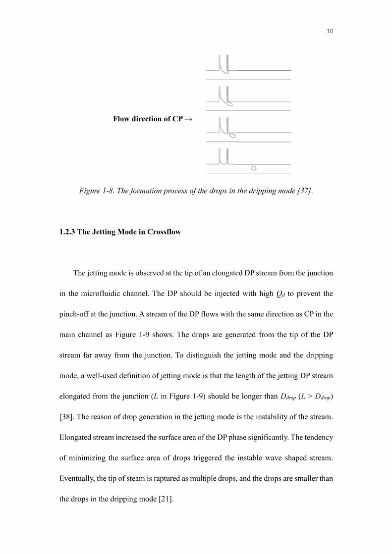
Flow direction of CP →
Figure 1-8. The formation process of the drops in the dripping mode [37].
1.2.3 The Jetting Mode in Crossflow
The jetting mode is observed at the tip of an elongated DP stream from the junction
in the microfluidic channel. The DP should be injected with high Qd to prevent the
pinch-off at the junction. A stream of the DP flows with the same direction as CP in the
main channel as Figure 1-9 shows. The drops are generated from the tip of the DP
stream far away from the junction. To distinguish the jetting mode and the dripping
mode, a well-used definition of jetting mode is that the length of the jetting DP stream
elongated from the junction (L in Figure 1-9) should be longer than Ddrop (L > Ddrop)
[38]. The reason of drop generation in the jetting mode is the instability of the stream.
Elongated stream increased the surface area of the DP phase significantly. The tendency
of minimizing the surface area of drops triggered the instable wave shaped stream.
Eventually, the tip of steam is raptured as multiple drops, and the drops are smaller than
the drops in the dripping mode [21].

11
Flow direction of CP →
L
Figure 1-9. The formation process of the drops in the jetting mode [37].
Modifying experimental conditions can change the patterns of drop generations,
even though using the same drop generation devices. In general, when the Qd is
increased, the pinch-off mode can be switched from the dripping mode to the jetting
mode.
1.3 The Models for Drop Sizes Prediction in Crossflow
According to the applications, the requirement of Ddrop can be different. It is
important to predict the size of products in the generation processes. From the studies
of the pinch-off modes in drop generation process, several models have been developed.
Three models from the view of applications and physical principles are introduced in
the section.

12
1.3.1 The Dimensionless Parameter-based Map
In the drop generation process, several controllable variables can be changed for a
chosen fluidic drop generator. Since the number of variables is already determined by
the design of the drop generator, it will be benefits to have reference values for Ddrop
prediction. A simple way is to calculate the dimensionless parameters from the
experimental data of Ddrop and controllable variables. The summarized plot of the
relationship between Ddrop and controllable variables can be used for checking the
experimental conditions to generate desired sized drops [36].
Figure 1-10 is an example of maps based on the dimensionless parameters. The
used device is a T-junction device with given geometries making drops in the squeezing
mode. Oil and water are used as the CP and DP, respectively. The controllable variables
of the drop generation system are the volume flow rate of the CP and DP (Qoil and
Qwater). Because of the shape of drops in the squeezing mode, two parameters, the length
and the width of the DP clog (L and w), are used to evaluate the size of the generated
drops.
Figure 1-10 summarized experimental data of the size of drops and the applied Qoil
and Qwater. The desired Ddrop can be found in the map, and the corresponding Qoil and
Qwater is the solution of the experimental conditions. The map is easy to use for
predicting Ddrop, but the data collection is necessary for every new design of drop
generator. Also, if the process of drop generation has been changed, such as the working
fluids have been replaced with different materials, the map is invalid. Experimental data

13
collection and the map plotting must be repeated.
Figure 1-10. An example of the dimensionless parameter-based map for drop
generation [36].
1.3.2 The Nondimensional Number-based Map
Nondimensional numbers are also used to predict the processes of drop generations.
From the previous discussion, the ranges of Ddrop in each pinch-off mode are different.
In the jetting mode, Ddrop is smaller than in the dripping mode. So the prediction of the
pinch-off mode can also related with Ddrop.
The dripping-to-jetting behavior of drop generation can be predicted by Capillary
number (Ca) and Weber number (We) [39-41]. Ca is considered as the ratio of viscos
drag force and the surface tension force, and We is the ratio of inertia force and the
surface tension force in the drop generation process. For example, smaller Ca means

14
that the viscos drag force acting on the drop generation process is smaller than the
surface tension force. The importance of the viscos drag force, the surface tension force,
and the inertia force acting on the system can be evaluated by these numbers.
Ca and We are calculated as Eq. (1-1) and Eq. (1-2) [42]. µc and µd are the dynamic
viscosity of the CP and the DP, respectively. Vc and Vd are the linear flow speed of the
CP and the DP, respectively. ρd is the density of the DP. Dneedle is the inner diameter of
the needle, which indicates the characteristic length in this equation. And, σ is the
interfacial tension between the CP and DP.
𝐶𝐶𝑎𝑎 = 𝜇𝜇𝑐𝑐𝑉𝑉𝑐𝑐𝜎𝜎
, (1-1)
𝑊𝑊𝑊𝑊 = 𝜌𝜌𝑑𝑑𝑉𝑉𝑑𝑑2𝐷𝐷𝑛𝑛𝑛𝑛𝑛𝑛𝑑𝑑𝑛𝑛𝑛𝑛𝜎𝜎
, (1-2)
For smaller Ca of the DP, drops are generated in the jetting mode because the effect
of shear stress acting on the stream of DP is relatively small. The drops cannot be
separated by CP from the position where DP meet with CP immediately. In a T-junction
device, the DP can grow continuously till the DP clogging the main channel. Based on
the explanation of the squeezing mode, DP drop only pinch-off when the pressure
difference acting on the both sides of the clog is high enough. However, the jetting
mode of drop generation can be related with bigger Ca [36]. Figure 1-11 is an example
of Ca and We from a membrane emulsification method. Each symbol in the map
indicates different working fluids as DP, and the hollow markers and the solid markers
mean the dripping mode and the jetting mode, respectively [21]. From the map, the
jetting mode always occur with high value of Ca and We.

15
Figure 1-11. An example of the nondimensional number-based map for drop generation
[21].
Another nondimensional number, Ohnesorge number (Oh), are used to evaluate the
difference of the dripping to jetting transition (DJT) in various fluids [21, 38]. Oh is the
ratio of viscous force and the square root of inertia force times surface tension force.
The Oh of CP can be calculated as Eq. (1-3).
𝑂𝑂ℎ𝐶𝐶𝐶𝐶 = 𝜇𝜇𝑐𝑐�𝜌𝜌𝑐𝑐𝐷𝐷𝑛𝑛𝑛𝑛𝑛𝑛𝑑𝑑𝑛𝑛𝑛𝑛𝛾𝛾
, (1-3)
Figure 1-12 shows the DJT of drop generation as Ca-We-Oh map. Oh of DP was
used in this map. The Ca-We-based map will be different for different OhDP [21, 38].
Different liquids were used for collecting data on the map, and the experimental setup
of this study is shown as Figure 1-13.

16
Figure 1-12. An example of Ca-We-Oh-based map for pinch-off modes [21].
Figure 1-13. The experimental setup for the Ca-We-Oh-based map example [21].
Another example of nondimensional number-based map is Figure 1-14. OhCP is
combined with Ca of CP (Caout in the map) as x-axis. We of DP (Wein in the map) is the
y-axis. The experimental setup of this study is shown as Figure 1-15, which is similar
with the previous example.

17
Figure 1-14. An example of Ca/Oh-We-based map for pinch-off modes [38].
Figure 1-15. The experimental setup for the Ca/Oh-We-based map example [38].
1.3.3 The Torque Balance Equation
Torque balance equation-based analysis (TBE) is another theoretical model for the
prediction of Ddrop [13, 27-29, 31, 43-45]. Figure 1-16 is a schematic figure of the TBE
model for membrane emulsification. The drop diameter is Dd at the surface of the
membrane. The DP is injected upwards and growing from the pore (diameter = Dp) as
height h, and the flow direction of CP is from left to right. Buoyance force (FBG),
dynamic lift force (FDL), Young-Laplace force (FYL), drag force (FDR), and interfacial

18
tension force (Fγ) are acting on the drop [12, 25, 29, 43, 46-51].
Figure 1-16. The schematic of TBE model in drop generation [43].
If the drop is considered as a rigid spherical object in the TBE model, point A is the
pivot point for the equilibrium of torque. Choosing 𝐷𝐷𝑝𝑝2
and ℎ − 𝐷𝐷𝑑𝑑2
as moment arms,
the TBE can be written as Eq. (1-4) to solve Ddrop [43].
𝐹𝐹𝐷𝐷𝐷𝐷 �ℎ −𝐷𝐷𝑑𝑑2� = �𝐹𝐹𝛾𝛾 − 𝐹𝐹𝑌𝑌𝑌𝑌 − 𝐹𝐹𝐷𝐷𝑌𝑌 − 𝐹𝐹𝐵𝐵𝐵𝐵�
𝐷𝐷𝑝𝑝2
, (1-4)
1.4 Rigid Body Motion Driven Crossflow-based Drop Generation
1.4.1 Motivation
Different drop generators in crossflow are introduced in the previous section, but
to build a drop generator with membrane emulsification or a microfluidic device in
laboratory has same challenges. Initial investment and maintenance are necessary. The

19
motivation of this study is to build a crossflow-based drop generation method in easier
way. The experimental conditions can be widely changed, and the parts of the generator
can be replaced.
From the studies of the drop generation methods introduced above, it is clear that
the shear force by the CP played important role in the pinch-off processes of drops [12,
21]. The shear force acting on the drops also can be applied by the rigid body motion
of the rotating continuous phase. This study is about using the shear force from the
rotational rigid body motion of CP to develop a drop generator with predictable Ddrop.
The Ddrop prediction will be discussed based on the models from the previous section.
1.4.2 Working Principle
Figure 1-17 shows the principle of the rigid body motion driven drops generation
system. The Vc is from CP with rigid body motion. When the radius of the rotational
rigid body motion is large enough, the flow direction of CP can be considered as linear
at the position where CP meet with DP. Similar with the design of membrane
emulsification, the DP is injected into CP in Qd at an angle θ. A needle was used to
inject the DP through a tubing, and the θ value was vertical to the flow direction of the
CP. In this research, θ = 90°.

20
Figure 1-17. The principle of the rigid body motion driven drops generation system.
The schematic figure of the drop generation method based on rigid body motion
was shown as Figure 1-18. The CP was filled a cylindrical container on a turntable. The
rotating motion of turntable caused the rotational rigid body motion of the CP. The
turntable was rotated by the AC/DC power supply. The DP was injected through a
syringe needle by a syringe pump. The tip of the syringe needle was perpendicularly
emerged under the free surface of the CP. Drops detached from the needle tip were
carried by the rotational motion of the CP. In the meantime, the drops were falling down
because of the gravity effects.
Figure 1-18. The schematic figure of the rigid body motion driven drops generation
system.
Since it was possible to change the factors of the system independently, such as
switching the rotating speed of the turntable or moving the position of the needle, the
versatility of the system was high. Wide-ranging size of drops released from the system

21
was available based on controlling these key components [30]. Further analysis
between the size of drop and each factor will be discussed based on the prototype of the
system. As an example of application, hydrogel beads will be generated from the system,
and the expansibility of the method will be considered.

22
Chapter 2 Methods and Materials
2.1 Materials
Mineral oil (Bluewater Chemgroup, 05089) and deionized water (DI water) were
used as the CP and the DP, respectively. They were filtered to remove particles or dusts
for better image quality. The properties of these two materials were measured as follows.
The density measurement was based on the Eq. (2-1).
𝜌𝜌 = 𝑚𝑚𝑉𝑉
, (2-1)
where m is the mass of the liquid sample, and V is the volume of the sample. A
micropipette (Eppendorf Research plus) was used to transport 1000 μL liquid sample
into a container on the electric weight (Scout Pro 400g). The mass of the liquid sample
was read from the electric weight (Table 2-1), and then the density of the liquid sample
was calculated. Measurement was repeated multiple times for each sample, and the
averaged value of the calculated density was used.

23
Table 2-1 The measurement results of mass (unit: g).
Mineral oil DI water
0.87 1.00
0.85 0.99
0.83 1.00
0.88 1.00
0.87 1.00
0.86
0.85
0.87
0.86
0.86
0.87
Average values
0.86 0.99

24
The viscosity measurement was done at 25 C° by using the rheometer (AR-1500EX)
with a cone geometry (60 mm diameter, 1°) and flow sweep function. The gap between
the geometry and the stage of the rheometer was filled with a measuring sample. The
controlling software of rheometer, TRIOS, can read the resistant from the screw rod
during rotating geometry. Figure 2-1 shows the viscosity measurement results. Both the
CP (mineral oil) and the DP (DI water) showed Newtonian fluid behaviors, because the
viscosities of the working fluids were constant in a wide shear rate range.
Figure 2-1. The viscosity measurement results of the rheometer.
The interfacial surface tension coefficient between the two liquids was measured
based on the pendant drop method [52-55] using a goniometer (Attension Theta
Goniometer). All of the measurements were operated at 22 C°, the room temperature.
A glass container filled with CP (mineral oil) was placed on the stage of the goniometer.
A DP (DI water) drop was formed in the oil using a syringe needle. The goniometer
captured the growth of the water drop and measured the surface tension coefficient by
processing the drop images. Based on the balanced forces acting on the drop, the

25
interfacial tension between DI water and mineral oil was calculated automatically by
the goniometer. Figure 2-2 shows the surface tension coefficient measurement results.
Most of the points with different volumes can be fitting on one single flat line. It means
that the surface tension coefficient between the mineral oil and the DI water is constant
for various sized drops. The outliers on the figure are caused by the reading error of the
goniometer during the image processing, so they can be ignored.
Figure 2-2. The interfacial surface tension coefficient measurement results of the
goniometer.
The measured fluid property values are summarized in Table 2-2.
Table 2-2. The measured properties of the CP and the DP.
DI water Mineral oil
Density ρ [kg/m3] 998 860
Viscosity μ [mPa∙s] 0.85 19.00
Surface tension σ [mN/m] 45

26
2.2 Experimental Setup
As Figure 2-3 shows, the experimental setup was built on an optical table. A 22 cm
diameter cylindrical transparent container (Imagitarium, Freshwater Aquarium, 2.2
gallon) was placed on a turntable (Pioneer Belt Drive Stereo Turntable, PL-112D) to be
used as the reservoir for the CP. The centers of the container and the turntable were
carefully aligned. The turntable could rotate the CP in the container in rigid body motion
at two different rotating speeds: Ω = 33.5 and 45.1 rounds per minute (rpm), which are
3.5 and 4.7 rad/s, respectively. The rotating speed was confirmed by a tachometer (DF
2234C+ Digital Photo Tachometer).
Figure 2-3. Experiment setup of drop generation.

27
The DP (DI water) was injected into the CP (mineral oil), through a syringe needle
by a syringe (BD 10 mL plastic syringe) using a syringe pump (Fusion 200, Chemyx
Inc). For different experimental conditions, the volume flow rate of the DP (Qd) was
applied at Qd = 0.1, 0.5, 1, 2, 4, 6, or 8 mL/min. A tubing (Tygon tubing, Cole-Parmer,
inner diameter: 0.020”, outer diameter: 0.060”) was used to deliver the DP from the
syringe to the needle. At the end of the tubing, a customized needle holder (Mechanical
parts, Makeblock) with a replaceable needle was fixed on a frame (OMA, McMaster-
Carr) standing on the optical table. Water levels were used to check the horizontality
and verticality of the needle holder.
Two kinds of 0.5”-long needle blunts with different inner diameters were used: SAI
23G needle (inner diameter: 0.0125”, outer diameter: 0.025”) or SAI 30G needle (inner
diameter: 0.0055”, outer diameter: 0.012” (SAI Infusion Technologies). The inner
diameters of the needles, Dneedle, was converted to 0.14 mm and 0.32 mm, respectively.
The needle tip was submerged 8 to 10 mm below the free surface of the CP to reduce
the disturbance from the needle hub. The linear velocity of the DP (Vd) was calculated
from Qd and Dneedle (𝑉𝑉𝑑𝑑 = 𝑄𝑄𝑑𝑑𝜋𝜋4𝐷𝐷𝑛𝑛𝑛𝑛𝑛𝑛𝑑𝑑𝑛𝑛𝑛𝑛
2 ). The tubing from syringe pump was inserted inside
the needle holder.
A reference ruler (Peel n Stick Removable Ruler Tape, Thermoweb) fixed on the
optical table was used to determine the position of the turntable. The distance from the
needle to the container center (i.e., the axis of rotation) (R) was adjusted to 40, 60, and
80 mm by moving the turntable back and forth with respect to the reference ruler. Thus,
the linear velocity of the CP at the needle tip (Vc) could be controlled by changing either

28
the distance or the needle-to-container-center rotating speed of the turntable (Vc = R∙Ω).
A high-speed camera (MIRO M310, Vision Research, Phantom) with a macro lens
(Canon, 100 mm, f1.x) was used to capture drop generation. The distance from the lens
to the needle holder was about 90 mm. For better imaging of the drop generation
processes, the camera was aligned on the line passing through the center of the container
and the needle, and the container was illuminated by a halogen lamp through a diffusion
paper. For consistent focusing, the relative positions between the needle and the camera
was fixed.
In summary, the established experimental setup enabled examining the drop
generation processes with various Dneedle, Vc, and Qd. Applied experimental conditions
are summarized in Table 2-3.
Table 2-3. The experimental conditions applied for the drop generation processes.
Dneedle [mm] 0.14 0.32
Qd [mL/min] 0.1 0.5 1 2 4 6 8
R [mm] 40 60 80
Ω [rad/s] 3.5 4.7
The experimental conditions were converted to Vc and Vd as shown in Table 2-3
and 2-4.

29
Table 2-4. Vc values [mm/s] calculated from the experimental conditions.
Ω [rad/s]
3.5 4.7
R [mm] 40 140.3 189.0
60 210.4 283.6
80 280.6 378.1
Table 2-5. Vd values [mm/s] calculated from the experimental conditions.
Dneedle [mm]
0.14 0.32
Qd [mL/min] 0.1 108.7 21.1
0.5 543.7 105.3
1 1087.3 210.5
2 2174.7 421.0
4 842.0
6 1263.1
8 1684.1

30
2.3 Experimental Procedures
Drop generation processes were investigated with the multiple experimental
conditions as shown in the previous section. For each condition, the turntable was
moved to the desired position of the R value with the container filled with the CP.
The next step was to prepare high-speed imaging. For most of the experiment, the
setting of the high-speed camera was 400 fps and 200 μs for the frame rate and exposure
time, respectively. The frame rate was adjusted to 40 fps for slow drop generation
processes with low Qd. The aperture number of the macro lens was set to 11-15 for
varies distances between the needle tip and the camera lens.
It was found that the cylindrical container distorted drop images due to its curved
surface. A reference image of a grid plate at chosen R was captured for image correction
before recording the drop generation processes. As Figure 2-4 shows, the grid plate was
placed at the position of the needle by a customized frame (Mechanical parts,
Makeblock). The grid plate was made by gluing a transparency film (APOLLO Laser
Printer Transparency Film) with printed 5 mm × 5 mm square grid patterns on a slide
glass (75 mm × 50 mm × 1.0 mm, Fisherbrand Plain Microscope Slides). A picture of
the grid plate was taken as Figure 2-5 shows to be used for the image process step later
on.

31
Figure 2-4. The grid plate attached on the needle holder for image correction.
Figure 2-5. A reference image of the grid plate in the continuous phase.
After reference image taking, the grid plate was replaced with the syringe of the
chosen Dneedle, and the turntable was set to the determined rotating speed Ω. The syringe
was filled with degassed DI water and connected to the needle holder via the tubing.
The syringe was placed on the syringe pump, and the determined Qd was input to the

32
syringe pump. After these steps to set the running conditions to desired values, the
preparation step of the experiment was finished.
For the experimental process, the turntable was turned on first. The selected
rotating speed could be achieved after 1- 2 rotations. Then the syringe pump was turned
on to inject the DP at chosen Qd. Several seconds were needed for the syringe pump to
reach the set value of Qd. After the steady generation of drops was observed, the process
was captured using the high-speed camera. Videos without undesired objects, such as
air bubbles remaining in the DP, were saved for processing.
The afore mentioned steps were repeated for different conditions.
2.4 Image Correction
The reason for having reference images of the grid plate was that the drops in the
captured images appeared to be stretched in the horizontal direction. Thus, the drops
seemed to be an ellipsoid, not a sphere as Figure 2-6 shows. This aspect ratio change of
the drop image was caused by the cylindrical wall of the container filled, which played
a role as a cylindrical lens. Therefore, it was required to calibrate the aspect ratio change
of the obtained images and to re-scale the images.

33
Figure 2-6. A raw image of drop generation processes (R = 80 mm, Ω = 4.7 rad/s,
and Qd = 0.5 mL/min.).
The reference images of the grid plate were used to calculate the elongated aspect
ratio. The reference images were read into ImageJ [56, 57] to measure the x and y
coordinates of intersection points of the grid. The coordinates were digitized from the
image. The brightness and contrast of the image were adjusted to identify the positions
of intersection points. For the purpose of convenience, the intersection points were
named as shown in Figure 2-7.

34
Figure 2-7. The x and y coordinates measurements of the intersection points from
the reference image.
Matlab (The MathWorks, Inc.,) was used for the following analysis of the measured
coordinates. According to the design of the printed patterns and the experimental setup,
the lines A1-D1, A2-D2, A3-D3, A4-D4, and A5-D5 should be horizontal, and the lines
A1-A5, B1-B5, C1-C5, and D1-D5 should be vertical in the image. The slopes of these
lines were calculated based on the trigonometric functions from measured coordinates
and converted to angles. To find the tilted angle of the recorded images (α), the angle
differences between the grid lines and the horizontal and vertical directions were
calculated and averaged as α.
Similarly, the x-y aspect ratios of the images were calculated from the measured
coordinates of the grid. Since grid shapes were square, the vertical segments from this
image should be same. The length of each segment was calculated, and then the aspect
ratio of the images (AR) was calculated as the ratio of the average length of vertical

35
segments to that horizontal segments.
The intersection coordinates, α, and AR, were measured for every reference image.
The results are summarized in Table 2-6. α and AR were used to corrrect the recorded
images using ImageJ. A cropped image from Figure 2-6 is shown in Figure 2-8 as an
example. The α and AR were calculated as 1.08° and 0.91, respectively. The image was
imported into ImageJ, and then rotated and rescaled. The corrected image is shown in
Figure 2-9. Compared with the raw image, the drops in the adjusted image look
spherical.
Table 2-6. The calculation results of tilted angles and elongated aspect ratios.
Dneedle [mm]
0.14 0.32
R [mm] 40 α = 0.72°, AR = 0.82 α = 1.14°, AR = 0.82
60 α = 0.31°, AR = 0.86 α = 0.90°, AR = 0.86
80 α = 1.08°, AR = 0.91 α = 0.74°, AR = 0.90
Figure 2-8. A cropped raw image of drop generation processes.
Figure 2-9. An adjusted image of drop generation processes.
36
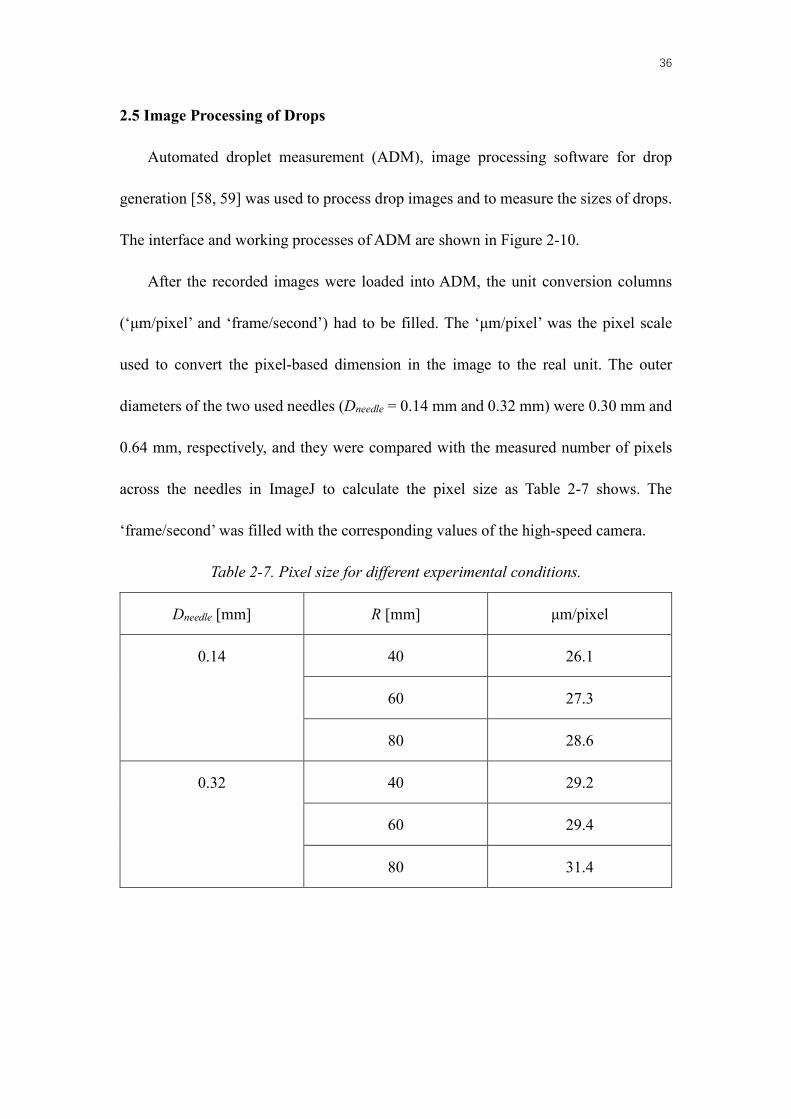
2.5 Image Processing of Drops
Automated droplet measurement (ADM), image processing software for drop
generation [58, 59] was used to process drop images and to measure the sizes of drops.
The interface and working processes of ADM are shown in Figure 2-10.
After the recorded images were loaded into ADM, the unit conversion columns
(‘μm/pixel’ and ‘frame/second’) had to be filled. The ‘μm/pixel’ was the pixel scale
used to convert the pixel-based dimension in the image to the real unit. The outer
diameters of the two used needles (Dneedle = 0.14 mm and 0.32 mm) were 0.30 mm and
0.64 mm, respectively, and they were compared with the measured number of pixels
across the needles in ImageJ to calculate the pixel size as Table 2-7 shows. The
‘frame/second’ was filled with the corresponding values of the high-speed camera.
Table 2-7. Pixel size for different experimental conditions.
Dneedle [mm] R [mm] μm/pixel
0.14 40 26.1
60 27.3
80 28.6
0.32 40 29.2
60 29.4
80 31.4

37

38
ADM compared every frame of the drop generation processes to automatically
extract a constant background image. The image with the background removed was
used for the following steps of the processing. The optimum image intensity value for
drop detection was determined by ADM’s binary threshold value finding function. Then,
ADM could detect the contours of drops from images. A single drop was traced over
frames, and its size was recorded for each frame. As a result, the diameters of multiple
drops were collected for this study. For each experimental condition, more than one
hundred drops were recorded (N > 100).
39
Chapter 3 Results
As briefly shown in the previous chapter, DI water drops were generated from the
needle tip with the rigid body rotation of the mineral oil in the container. This result
justifies the assumption that the rigid body motion of the CP created shear force to
separate drops from the vertically injected DP. Multiple spherical drops with similar
diameters were continuously released from the needle tip. It was observed that the drops
generation process achieved steady state. The diameter of the generated drops could be
controlled by adjusting the velocities of the CP and the DP, Vc and Vd.
3.1 Experimental Images and Drop Pinch-off Modes of the Drops
The pinch-off modes of generated drops were different depending on experimental
conditions. The drop generation modes in cross-flow are classified as the squeezing,
dripping, and jetting mode [2]. The squeezing mode, which can occur in microfluidic
drop generators, was not observed in this study [36]. The other two modes were
observed with different experimental conditions.
Figures 3-1 and 3-2 show the examples of the two drop generation modes. The
experimental conditions were Dneedle = 0.14 mm, Vc = 210.4 mm/s and Vd = 543.7 mm/s,
and Vc = 210.4 mm/s and Vd = 2174.7 mm/s, respectively.
In Figure 3-1, the pinch-off occurred at the needle tip, which is recognized as the
dripping mode. In Figure 3-2, it is clear that the distance from the needle tip to the

40
pinch-off location exceeded Ddrop (L > Ddrop) [38]. Therefore, it was observed that
changing Vd only can cause change in the pinch-off mode.
Figure 3-1. The drop generation process of Vc = 210.42 mm/s, and Vd = 543.67 mm/s.
Figure 3-2. The drop generation process of Vc = 210.42 mm/s, and Vd = 2174.68
mm/s.

41
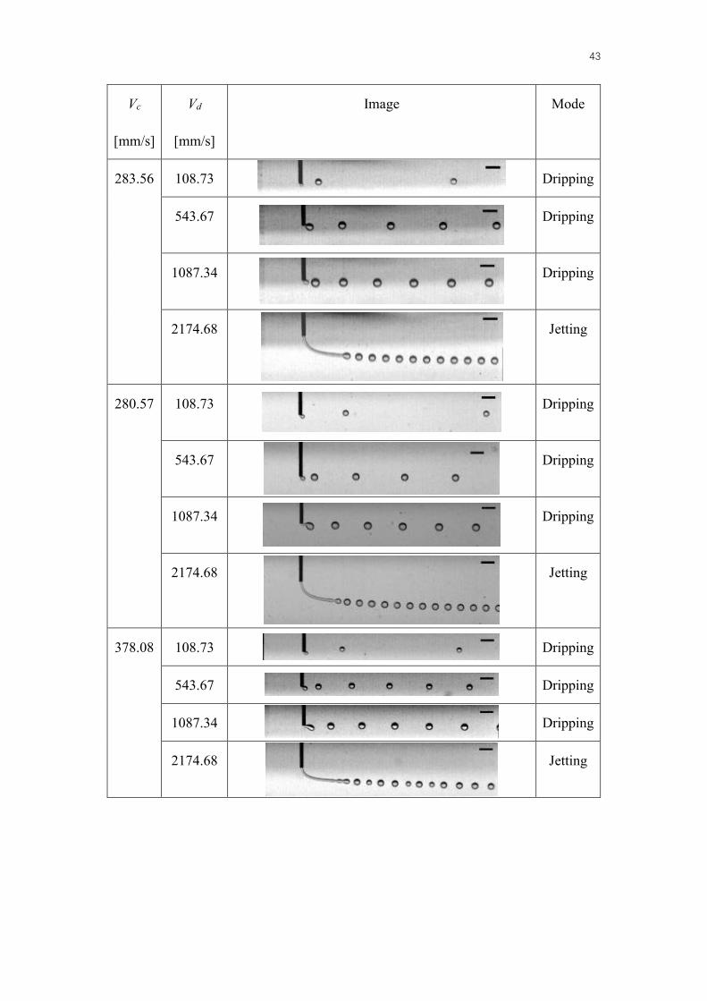
Based on the definitions of the modes, it was possible to distinguish the pinch-off
modes for all cases. By summarizing the results, the images with varies Vc and Vd
were illustrated as Table 3-1 and 3-2.
Table 3-1. Drop generations with Dneedle = 0.14 mm (scale bar = 1 mm).
Vc
[mm/s]
Vd
[mm/s]
Image Mode
140.28
108.73
Dripping
543.67
Dripping
1087.34
Dripping
2174.68
Jetting
(Continued)

42
Vc
[mm/s]
Vd
[mm/s]
Image Mode
189.04 108.73
Dripping
543.67
Dripping
1087.34
Dripping
2174.68
Jetting
210.42 108.73
Dripping
543.67
Dripping
1087.34
Dripping
2174.68
Jetting
(Continued)
43
Vc
[mm/s]
Vd
[mm/s]
Image Mode
283.56 108.73
Dripping
543.67
Dripping
1087.34
Dripping
2174.68
Jetting
280.57 108.73
Dripping
543.67
Dripping
1087.34
Dripping
2174.68
Jetting
378.08 108.73 Dripping
543.67 Dripping
1087.34
Dripping
2174.68
Jetting

44
Table 3-2. Drop generations with Dneedle = 0.32 mm (scale bar = 1 mm).
Vc
[mm/s]
Vd
[mm/s]
Image Mode
140.28 21.05
Dripping
105.26
Dripping
210.51
Dripping
421.02
Dripping
842.04
Dripping
1263.06
Jetting
1684.08
Jetting
(Continued)
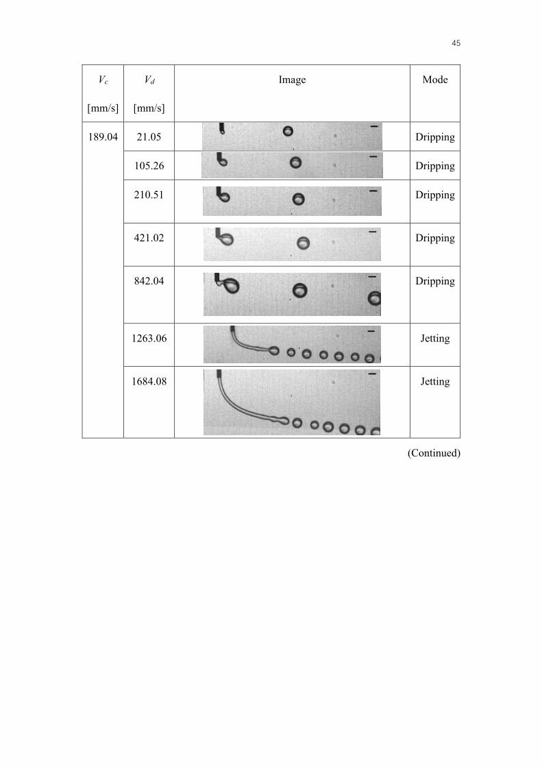
45
Vc
[mm/s]
Vd
[mm/s]
Image Mode
189.04 21.05
Dripping
105.26
Dripping
210.51
Dripping
421.02
Dripping
842.04
Dripping
1263.06
Jetting
1684.08
Jetting
(Continued)
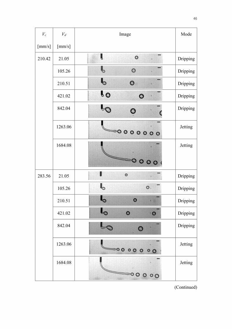
46
Vc
[mm/s]
Vd
[mm/s]
Image Mode
210.42 21.05
Dripping
105.26
Dripping
210.51
Dripping
421.02
Dripping
842.04
Dripping
1263.06
Jetting
1684.08
Jetting
283.56 21.05 Dripping
105.26
Dripping
210.51
Dripping
421.02
Dripping
842.04
Dripping
1263.06
Jetting
1684.08
Jetting
(Continued)
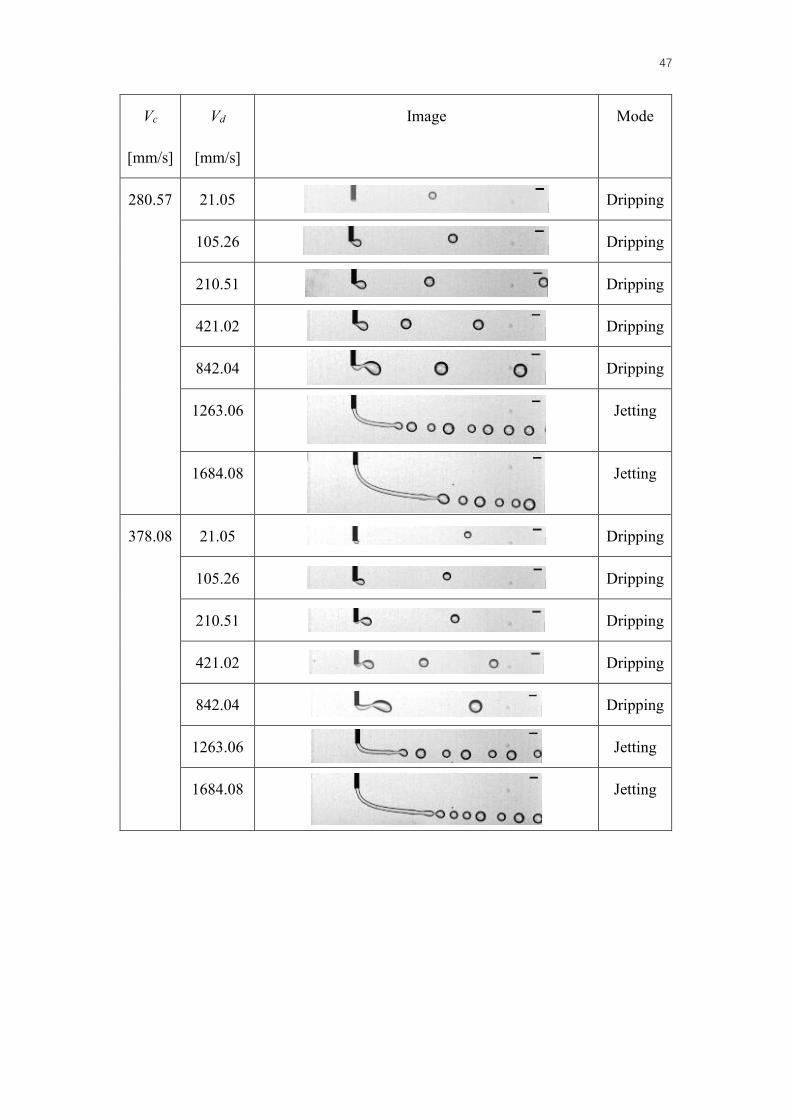
47
Vc
[mm/s]
Vd
[mm/s]
Image Mode
280.57 21.05 Dripping
105.26 Dripping
210.51 Dripping
421.02 Dripping
842.04
Dripping
1263.06
Jetting
1684.08
Jetting
378.08 21.05 Dripping
105.26 Dripping
210.51 Dripping
421.02 Dripping
842.04 Dripping
1263.06
Jetting
1684.08
Jetting

48
3.2 Drop Diameter Distribution
As introduced in the previous section, the diameters of generated drops (Ddrop) were
automatically measured using ADM. The average and standard deviation values of Ddrop
with various combinations of Vc and Vd are summarized in Table A-1. Because of the
low frequency of drops generations, the ADM analysis of the images from Vc = 140.28
mm/s, Vd = 21.05 mm/s and Vc = 189.04 mm/s, Vd = 21.05 mm/s was not able to be
produced.
Because the goal of this study is to generate monodisperse drops continuously, it is
important to narrow down the range of the Ddrop to certain experimental conditions. For
this purpose, the histograms of drops sizes were plotted using the measured Ddrops [60].
Figure 3-3 shows an example of the histogram to compare drop size distributions
between two different Vc values (Vc = 140.3 mm/s: blue, and 189.0 mm/s: red) with
same Vd = 543.7 mm/s, and Dneedle = 0.14 mm. The x-axis was the range of Ddrop. For
Dneedle = 0.14 mm experiments, the interval was chosen as 2 μm to have the optimum
view of the plots. The y-axis was the probabilities of each range of the diameter values.
With these conditions, drops were generated in the dripping mode. Accordingly, the
histogram shows narrow drop size distribution with only one peak for each case.
Therefore, the generated drops in the experimental conditions were well controlled.

49
Figure 3-3. Drop size distribtion of Vc = 140.3 mm/s or 189.0 mm/s, Vd = 543.7 mm/s,
Dneedle = 0.14 mm.
Figure 3-4 shows another example: Vc = 140.3 mm/s (blue) or 189.0 mm/s (red),
Vd = 2174.7 mm/s, and Dneedle = 0.14 mm. As shown previously, higher Qd was applied
for these experimental conditions (i.e., higher Vd), the pinch-off mode was the jetting
mode.
Compared with Figure 3-3, the most significant difference found in Figure 3-4 is
the number of the peaks. In contrast to on single sharp peak of the dripping mode,
multiple peaks are found in the jetting mode. This appears to be due to the Rayleigh-
Plateau instability which causes pinch-off in the jetting mode. As the jet stream of the
DP got longer, surface tension developed this wavy instability. Thus, the pinch-off
occurring at the stream tip more randomly, which resulted in multiple peaks [12].

50
Figure 3-4. The histograms of Vc = 140.28 mm/s or 189.04 mm/s, Vd = 2174.68 mm/s,
Dneedle = 0.14 mm.
All histograms of Dneedle = 0.14 mm and 0.32 mm are shown in Table B-1 and B-2,
respectively. As references, the pinch-off modes are noticed in the tables.
The coefficient of variation (CV) of drop size was used to evaluate the
monodispersity of generated drops based on the Eq. (3-1), (3-2), and (3-3) [2, 24].
Standard deviation of 𝐷𝐷𝑑𝑑𝑑𝑑𝑑𝑑𝑑𝑑: STD𝐷𝐷𝑑𝑑𝑑𝑑𝑑𝑑𝑝𝑝 = �1𝑛𝑛∑ �𝐷𝐷𝑑𝑑𝑑𝑑𝑑𝑑𝑑𝑑,𝑖𝑖 − 𝐷𝐷𝑑𝑑𝑑𝑑𝑑𝑑𝑑𝑑��������
2𝑛𝑛𝑖𝑖=1 , (3-1)
Mean of 𝐷𝐷𝑑𝑑𝑑𝑑𝑑𝑑𝑑𝑑: 𝐷𝐷𝑑𝑑𝑑𝑑𝑑𝑑𝑑𝑑������� = 1𝑛𝑛∑ 𝐷𝐷𝑑𝑑𝑑𝑑𝑑𝑑𝑑𝑑,𝑖𝑖𝑛𝑛𝑖𝑖=1 , (3-2)
CV [%] = STD𝐷𝐷𝑑𝑑𝑑𝑑𝑑𝑑𝑝𝑝𝐷𝐷𝑑𝑑𝑑𝑑𝑑𝑑𝑝𝑝��������� × 100, (3-3)
The values of CV were calculated for each experimental condition individually.
The detailed calculated results of CV are shown in Table B-3. The generated drops
showed different ranges of CV in the dripping mode and in the jetting mode as 0.21 ~
51
6.8 % and 1.1 ~ 14.9 %, respectively. Because polydispersed drops were generated in
the jetting mode, the values of CV in the jetting mode are higher than the values in the
dripping mode.
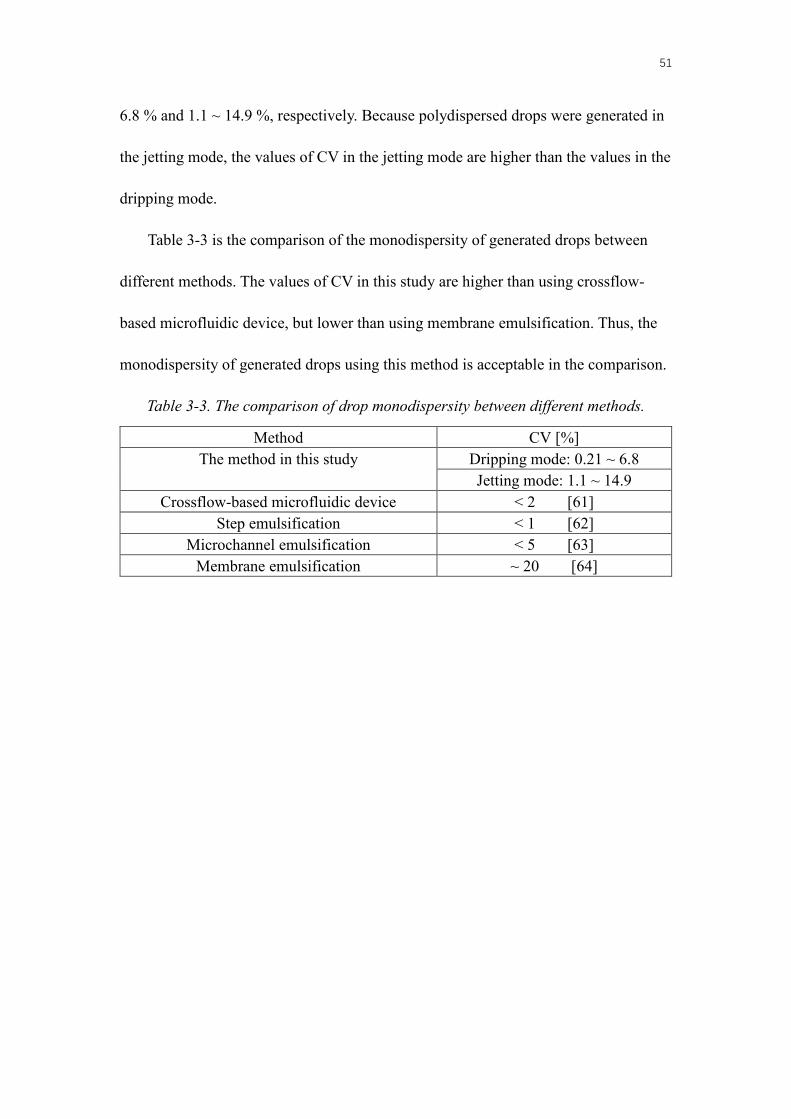
Table 3-3 is the comparison of the monodispersity of generated drops between
different methods. The values of CV in this study are higher than using crossflow-
based microfluidic device, but lower than using membrane emulsification. Thus, the
monodispersity of generated drops using this method is acceptable in the comparison.
Table 3-3. The comparison of drop monodispersity between different methods.
Method CV [%] The method in this study Dripping mode: 0.21 ~ 6.8
Jetting mode: 1.1 ~ 14.9 Crossflow-based microfluidic device < 2 [61]
Step emulsification < 1 [62] Microchannel emulsification < 5 [63]
Membrane emulsification ~ 20 [64]

52
3.3 Dimensionless Phase Diagram of the Drop Generation
It is useful to present the obtained data in a dimensionless map for predicting drop
generation mode and size [36]. As such Vd/Vc and Ddrop/Dneedle are natural choices for
ploting a dimensionless map of this study. The numeric values of Vd/Vc and Ddrop/Dneedle
are summarized in Table C-1.
A dimensionless map for Dneedle = 0.14 mm is shown in Figure 3-5. Based on the
discussion in the previous sections, drops in different pinch-off modes were indicated
in the map with different markers as the legends of Figure 3-5 shown. Different markers
were used as the figure shown. The hollow markers and the solid markers were
indicating the dripping mode zone and the jetting mode zone, respectively.

53
54
3.4 The Different Pinch-off Zones in the Nondimensional Analysis Phase Diagram
In Figure 3-5, it was possible to separate the map as two zones, the dripping mode
zone and the jetting mode zone. The markers with the same colors were indicating the
same values of Qd. Boundaries of each zone were identified by connecting these
markers as straight lines. As Figure 3-6 shows, the hollow markers and the solid
markers indicated the pinch-off modes of drops as the dripping mode and the jetting
mode, respectively. A boundary between these two zones as the DJT was not
identified in current experiments. It will be a part of the future work of this study.
From the map, it was clear that for higher Vd, the ratio of Ddrop and Dneedle was
increased. If the same needles were used, Ddrop was increasing with Vd in the dripping
mode zone. If the Vd was higher than the criteria value, the pinch-off mode became
the jetting mode. The ratio of Ddrop and Dneedle was slightly decreased for the
experimental conditions with fixed Vc. By knowing the experimental conditions, the
pinch-off zone of drop generation processes in the map was predictable.

55

56
3.5 The Application of the Nondimensional Analysis Phase Diagram
The map was supposed to be a reference of drop size predictions. For different
experimental conditions, if the coordinates of the data were closed to each other in the
map, the pinch-off processes and the diameters of the drops should be similar.
Figure 3-7 was an example of the predictions of the drop generations. 3 different
positions on the map were chosen. The images of the drop generation processes closed
to the positions were illustrated for comparison. The experimental conditions for each
image were included in the map. As the figure shown, the products of drops were similar,
even the experimental conditions for the drop generations were different.
In this map, data points in the jetting mode are in one line with narrow range. It is
possible to predict Ddrop easily with known experimental conditions if the pinch-off
mode of drop generation is jetting mode. But the prediction does not work well for
drops in the dripping mode because of the widely range of data points in the dripping
mode zone. Currently, the data points in the dripping mode zone can be used as
references of produced Ddrop with same experimental condition. For the purpose of
predicting Ddrop with arbitrary experimental conditions, building scaling laws will be
considered as future works.

57

58
Chapter 4 Discussion
4.1 Absence of the Squeezing Mode
In this study, only the dripping and jetting mode were observed whereas the
squeezing mode was not. The absence of the squeezing mode can be explained as
follows.
When the DP is injected into the T-junction device, the tip of the DP stream enters
the junction and is elongated through the channel. Because the tip of the DP stream
clogs the channel, pressures on each side of the stream are different. As the DP grows
in the channel, the pressure difference also increases. Eventually, the pressure different
becomes large enough to break the DP stream into a drop confined by the channel wall.
Therefore, the main factor of the squeezing mode in the T-junction device is the pressure
difference, and the boundary walls of the microfluidic channel play critical roles to
cause the clogging of the channel by the DP [36].
In the present study, however there was no surrounding geometry which could
confine the flow of the DP. As a result, the squeezing mode did not occur in the current
system.
4.2 Controlling Drop Diameter
In this study, it was possible to modulate drop sizes. It was clear that increase in Vc
generated smaller drops in the dripping modes. This is because as Vc increased, drag on

59
the drop growing at the needle tip increased, which drives the pinch-off processes of
drops. Also, the drops were allowed shorted time for the growth before pinch-off.
For the changing of Vd, Ddrop increased when higher Vd was applied in the dripping
modes. If the Vc was fixed, the allowed time of drop growth before pinch-off was the
same. Higher Vd was able to apply more amount of the DP into the drop. In this case,
Ddrop had included more liquid than the drop can have with lower Vd, Ddrop would be
bigger.
As Vd increased, a neck could be observed between the needle tip and the generated
drop, which indicates that the pinch-off mode was switching from the dripping mode
to the jetting mode. Once Vd was high enough, the jetting mode became prevalent and
Ddrop had decreased compared with the dripping mode [21, 38, 42] .
In the jetting mode, instability developed along the elongated DP stream in the CP.
Because of the significantly increased surface area and the tendency of the DP to
minimize the surface area, unstable wavy shapes occur among the stream. Eventually,
the tip of the stream was ruptured into drops. In the jetting mode, the shear force was
not the main driving force of drop generations, and thus changing Vc could not change
Ddrop so much.

60
4.3 Nondimensional Numbers in the Drop Generation Processes
Nondimensional numbers, Ca and We, are also used to predict drop generation
modes [21, 38, 42]. These numbers were calculated based on Eq. (1-1) and (1-2), and
the numerical values are shown in Table D-1.
A dimensionless map of Ca and We is plotted in Figure 4-1. Here, the hollow and
solid markers indicate the dripping and jetting mode, respectively. From the previous
discussion, the jetting mode occurs for higher Ca and We. Because of the limited
experimental data, the dependent with Ca and the DJT is not clear in the map. The
jetting mode is only identified in the map with high We.
By the comparison between several specific images, the boundary of the dripping
mode and jetting mode zones can be assumed. As Figure 4-2 shows, the length of the
DP stream between the needle tip and the pinch-off drop is increased with Ca increasing.
The experimental result of Qd = 4 mL/min and Vc = 376.9 mm/s is very close to the
jetting mode. From this comparison, a hypothesis is that the jetting mode related with
Ca. For higher Ca, the jetting mode should occur. More experiments will be considered
for supporting the assumption as future works.

61
62

63
Considering the effect of Oh [2, 21, 38], OhCP and the value of Ca/OhCP are
calculated as Table D-2. Figure 4-3 is the Ca/Oh-We-based map from the calculation
results. The map can be compared with the frame in Figure 4-4 with same range [38].
The jetting mode occur in high We for both Figure 4-3 and 4-4, but the values of We at
DJT are different. DJT can be found at We = 10 and We =1, respectively. A possible
reason of this difference is the experimental setup. For the data in Figure 4-3, because
rotational rigid body motion of CP was used for the shear force, CP was considered as
uniform flow. However, for the data in Figure 4-4, CP was applied through a cylindrical
channel with wall shear stress. Following studies of the DJT difference will be
considered as future works.

64

65

66
4.4 Drop Size Predictions in Torque Balance Equation
As the introduction shows, torque balance equation (TBE) is another way to
predict Ddrop from the experimental conditions [13, 27-29, 31, 43-45]. TBE is a model
based on the drops generated in the dripping mode. Drops are pinched off when the
torques of forces acting on the drop reached balanced state. Drops in the jetting mode
cannot be predicted by TBE because of different process of pinch-off.
Figure 4-5 is the schematic figure of the TBE in this study. The drop is pinched
off from the joint. Drag force (FDR), surface tension force (Fγ), Young-Laplace force
(FYL), buoyancy force (FBG), and gravity (FG) are calculated as Eq. (4-1) to Eq. (4-5),
respectively [12, 25, 29, 43, 46-51]. CD and Adrop in Eq. (4-1) are the drag coefficient
and the cross-section area of the drop, Vdrop in Eq. (4-4) and Eq. (4-5) are the volume
of the drop, respectively. The drop is assumed as spherical shape without deformation.
𝐹𝐹𝐷𝐷𝐷𝐷 = 𝐶𝐶𝐷𝐷𝐴𝐴𝑑𝑑𝑑𝑑𝑑𝑑𝑑𝑑𝜌𝜌𝑐𝑐𝑉𝑉𝑐𝑐2
2, (4-1)
𝐹𝐹𝛾𝛾 = 𝜋𝜋𝐷𝐷𝑛𝑛𝑛𝑛𝑛𝑛𝑑𝑑𝑛𝑛𝑛𝑛𝛾𝛾, (4-2)
𝐹𝐹𝑌𝑌𝑌𝑌 = 𝛾𝛾𝐷𝐷𝑑𝑑𝑑𝑑𝑑𝑑𝑝𝑝
𝜋𝜋𝐷𝐷𝑛𝑛𝑛𝑛𝑛𝑛𝑑𝑑𝑛𝑛𝑛𝑛2 , (4-3)
𝐹𝐹𝐵𝐵𝐵𝐵 = 𝜌𝜌𝑐𝑐𝑔𝑔𝑉𝑉𝑑𝑑𝑑𝑑𝑑𝑑𝑑𝑑, (4-4)
𝐹𝐹𝐵𝐵 = 𝜌𝜌𝑑𝑑𝑔𝑔𝑉𝑉𝑑𝑑𝑑𝑑𝑑𝑑𝑑𝑑, (4-5)

67
Figure 4-5. The schematic figure of TBE in this study.
Dynamic life force is not considered because the shear rate is 0 for uniform flow
of CP. The inertia force of DP is ignored based on the assumption that the pressure
different because of DP at the needle tip is smaller than the Laplace pressure at the
curved surface of DP [43].
For CD, different values are used in literatures. Either a Reynolds number related
equation or a correction factor for specific experimental setup are determined [23, 38,
42, 60]. In this study, the drag coefficient of sphere, CD = 0.47, was used.
As the figure shows, the arms of forces are simplified as 𝐷𝐷𝑛𝑛𝑛𝑛𝑛𝑛𝑑𝑑𝑛𝑛𝑛𝑛2
and 𝐷𝐷𝑑𝑑𝑑𝑑𝑑𝑑𝑝𝑝2
,
respectively. The TBE for this study is summarized as Eq. (4-6) [43].
𝐹𝐹𝐷𝐷𝐷𝐷𝐷𝐷𝑑𝑑𝑑𝑑𝑑𝑑𝑝𝑝2
= �𝐹𝐹𝛾𝛾 − 𝐹𝐹𝑌𝑌𝑌𝑌 − 𝐹𝐹𝐵𝐵 + 𝐹𝐹𝐵𝐵𝐵𝐵�𝐷𝐷𝑛𝑛𝑛𝑛𝑛𝑛𝑑𝑑𝑛𝑛𝑛𝑛
2, (4-6)
Substituting the known values based on different experimental conditions, Ddrop
can be solved from Eq. (4-6). Imaginary roots and root do not meaningful, such as Ddrop
= Dneedle, are ignored. The chosen solutions of Ddrop in different experimental conditions
are summarized as Table E-1.
68
The solved Ddrop were introduced in the dimensionless map to compare with the
experimental data as Figure 4-6 and 4-7. Solved Ddrop were plotted with
corresponding experimental conditions of Dneedle, Vd, and Vc. The solid lines
connected the experimental data of Ddrop with dripping modes, and the dashed lines
indicates Ddrop solved from TBE.
From the experimental data, Ddrop increased with Vd. But this relationship is not
shown in Ddrop solved from TBE. The reason is the lack of Vd in the equation of TBE.
Only Vc is included in the term of drag force, so the result changing because of Vd
cannot be presented.
Also, the solved Ddrop showed difference between the experimental data, which
may cause by the model of TBE. TBE is based on one assumption that no deformation
occurs during the pinch-off process. The drop is considered as a rigid sphere with
forces acting on it. It is not true because fluid cannot maintain the shape under
stresses. When forces are acting on the drop, the drop will deform and flow away.
Since the model ignored the nature of fluid, Ddrop solved from TBE can have
limitation for drop size predictions.

69
70

71
Chapter 5 Conclusion
In this study, a cross-flow based drop generator was developed based on the CP in
rotational rigid body motion. The DP was injected into the CP through a needle
perpendicularly to the motion of the CP. Shear force because of the rotational motion
of CP generated drops of DP in the setup. Also, the range of Ddrop can be changed by
applying different experimental conditions.
Two different pinch-off modes, the dripping mode and the jetting mode, were
observed in the system with different experimental conditions. The jetting mode can
occur with high Vd. In the dripping mode, drops were detached from the needle tip one
by one. In the jetting mode, drops were generated from the rapture of elongated DP
stream in the CP. Increased surface area of DP and the tendency of DP to minimize the
surface area caused the wavy shape of the DP stream. Eventually the unstable DP stream
raptured as multiple drops. Comparing with the drops in the dripping modes, the drops
in the jetting modes were smaller and not monodispersed.
Software ADM was used to measure Ddrop from captured images. The
monodispersity of generated drops were compared with other methods. Drops were
monodispersed in the dripping mode than in the jetting mode, and drops generated in
both of these modes were acceptable.
Nondimensional analysis phase diagram map, Vd/Vc and Ddrop/Dneedle, was used to
predict Ddrop with known experimental conditions. It was possible to check the Ddrop
from the map as reference values.
Ca, We, and Oh were studied to predict the pinch-off mode. For higher Ca and We,

72
jetting mode will occur. The specific DJT for different pairs of CP and DP are different.
Oh can be used to understand the effect of different fluids. It was possible to predict the
pinch-off mode from the experimental conditions.
The DJT in Ca-We-Oh-based map was different with references. The reason can be
the difference between experimental setups. Following studies will be considered as
future works.
Also, Ddrop solved from TBE were compared with experimental data. TBE showed
limitations of Ddrop prediction. The difference between TBE solved results and
experimental data can caused by the assumption of TBE. As a conclusion, TBE does
not work well for the setup in this study.
In summary, it was possible to make different sized drops by controlling the
experimental conditions of the setup. In future, applications of making hydrogel beads
with controllable sized are considered [65, 66]. Solutions of hydrogel will be used as
the DP. By changing the experimental conditions, various sizes of hydrogel solution
drops can be generated. After gelation process, hydrogel beads can be collected from
the setup.
73
Appendix A. The Measurement Results of Drop Sizes
Table A-1. The drop diameters with various experimental conditions.
Vc [mm/s] Vd [mm/s] Ddrop [μm] (mean ± std)
140.28 108.73 625.70 ± 14.25
543.67 797.43 ± 5.03
1087.34 896.16 ± 51.10
2174.68 734.26 ± 34.33
189.04 108.73 549.29 ± 4.27
543.67 712.96 ± 3.55
1087.34 758.01 ± 3.39
2174.68 659.41 ± 58.69
210.42 108.73 513.71 ± 7.67
543.67 657.59 ± 8.88
1087.34 686.41 ± 3.58
2174.68 636.90 ± 39.19
283.56 108.73 477.83 ± 2.97
543.67 561.57 ± 2.57
1087.34 668.54 ± 24.89
2174.68 546.48 ± 21.58
(Continued)

74
Vc [mm/s] Vd [mm/s] Ddrop [μm] (mean ± std)
280.57 108.73 482.51 ± 3.10
543.67 567.64 ± 3.72
1087.34 642.92 ± 25.65
2174.68 552.62 ± 20.16
378.08 108.73 476.73 ± 3.24
543.67 494.73 ± 1.77
1087.34 583.79 ± 5.70
2174.68 541.30 ± 5.89
140.28 105.26 1853.60 ± 68.88
210.51 2016.70 ± 7.49
421.02 2135.40 ± 11.55
842.04 2187.40 ± 149.60
1263.06 1554.40 ± 75.65
1684.08 1661.40 ± 196.32
189.04 105.26 1622.00 ± 4.87
210.51 1725.70 ± 4.97
421.02 1826.60 ± 5.65
842.04 2078.50 ± 12.46
1263.06 1402.20 ± 83.56
1684.08 1479.50 ± 220.48
(Continued)

75
Vc [mm/s] Vd [mm/s] Ddrop [μm] (mean ± std)
210.42 21.05 1119.50 ± 4.31
105.26 1376.40 ± 6.42
210.51 1530.60 ± 18.64
421.02 1605.40 ± 4.55
842.04 1849.70 ± 8.82
1263.06 1241.60 ± 34.83
1684.08 1384.70 ± 172.51
283.56 21.05 888.20 ± 14.30
105.26 1071.30 ± 10.83
210.51 1196.60 ± 10.00
421.02 1298.00 ± 32.52
842.04 1743.20 ± 35.42
1263.06 1112.70 ± 122.39
1684.08 1223.80 ± 144.82
(Continued)
76
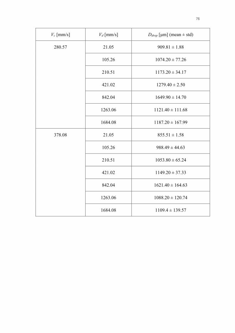
Vc [mm/s] Vd [mm/s] Ddrop [μm] (mean ± std)
280.57 21.05 909.81 ± 1.88
105.26 1074.20 ± 77.26
210.51 1173.20 ± 34.17
421.02 1279.40 ± 2.50
842.04 1649.90 ± 14.70
1263.06 1121.40 ± 111.68
1684.08 1187.20 ± 167.99
378.08 21.05 855.51 ± 1.58
105.26 988.49 ± 44.63
210.51 1053.80 ± 65.24
421.02 1149.20 ± 37.33
842.04 1621.40 ± 164.63
1263.06 1088.20 ± 120.74
1684.08 1109.4 ± 139.57

77
Appendix B. The Size Distributions of Generated Drops
Table B-1. The histograms of experiments with Dneedle = 0.14 mm.
Vc [mm/s]
Vd [mm/s]
140.28
189.04
Mode
108.73
Dripping
543.67
Dripping
(Continued)
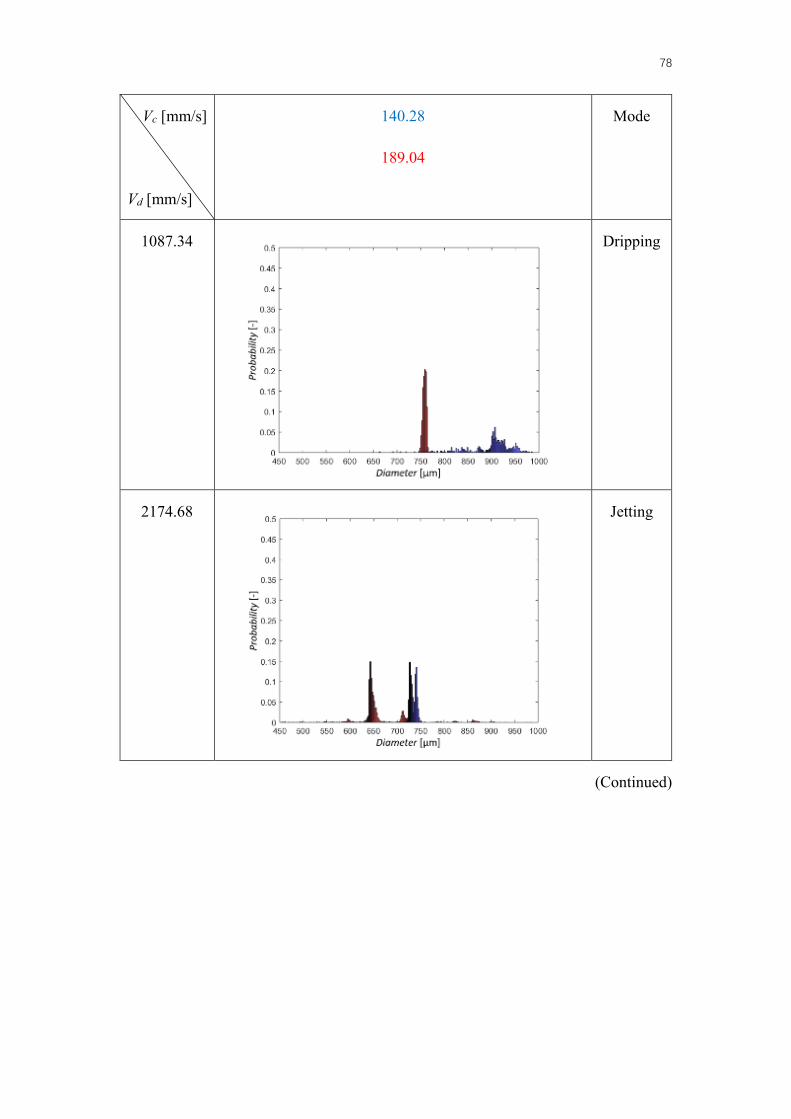
78
Vc [mm/s]
Vd [mm/s]
140.28
189.04
Mode
1087.34
Dripping
2174.68
Jetting
(Continued)

79
Vc [mm/s]
Vd [mm/s]
210.42
283.56
Mode
108.73
Dripping
543.67
Dripping
(Continued)

80
Vc [mm/s]
Vd [mm/s]
210.42
283.56
Mode
1087.34
Dripping
2174.68
Jetting
(Continued)

81
Vc [mm/s]
Vd [mm/s]
280.57
378.08
Mode
108.73
Dripping
543.67
Dripping
(Continued)

82
Vc [mm/s]
Vd [mm/s]
280.57
378.08
Mode
1087.34
Dripping
2174.68
Jetting

83
Table B-2. The histograms of experiments with Dneedle = 0.32 mm.
Vc [mm/s]
Vd [mm/s]]
140.28
189.04
Mode
105.26
Dripping
210.51
Dripping
421.02
Dripping
(Continued)

84
Vc [mm/s]
Vd [mm/s]]
140.28
189.04
Mode
842.04
Dripping
1263.06
Jetting
1684.08
Jetting
(Continued)

85
Vc [mm/s]
Vd [mm/s]]
210.42
283.56
Mode
21.05
Dripping
105.26
Dripping
210.51
Dripping
(Continued)

86
Vc [mm/s]
Vd [mm/s]]
210.42
283.56
Mode
421.02
Dripping
842.04
Dripping
1263.06
Jetting
(Continued)

87
Vc [mm/s]
Vd [mm/s]]
210.42
283.56
Mode
1684.08
Jetting
Vc [mm/s]
Vd [mm/s]]
280.57
378.08
Mode
21.05
Dripping
105.26
Dripping
(Continued)

88
Vc [mm/s]
Vd [mm/s]]
280.57
378.08
Mode
210.51
Dripping
421.02
Dripping
842.04
Dripping
(Continued)

89
Vc [mm/s]
Vd [mm/s]]
280.57
378.08
Mode
1263.06
Jetting
1684.08
Jetting
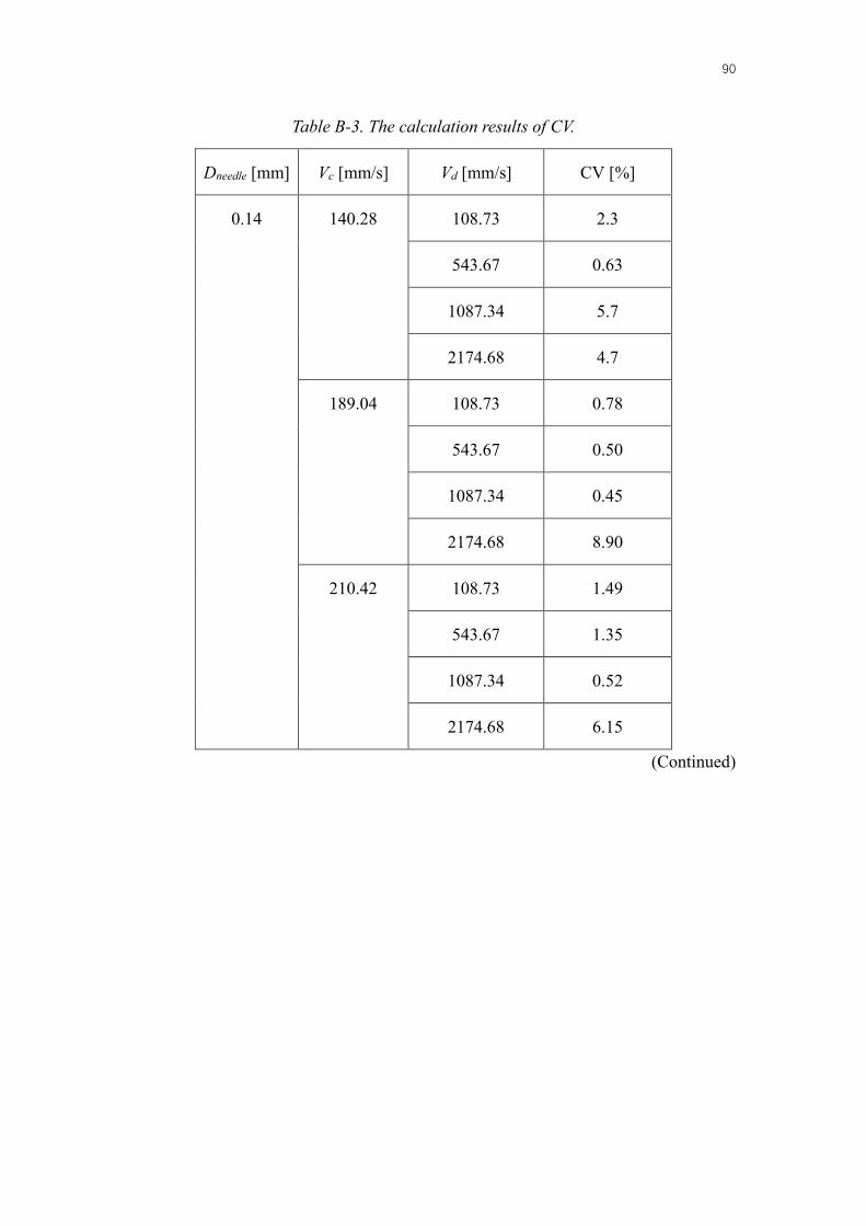
90
Table B-3. The calculation results of CV.
Dneedle [mm] Vc [mm/s] Vd [mm/s] CV [%]
0.14 140.28 108.73 2.3
543.67 0.63
1087.34 5.7
2174.68 4.7
189.04 108.73 0.78
543.67 0.50
1087.34 0.45
2174.68 8.90
210.42 108.73 1.49
543.67 1.35
1087.34 0.52
2174.68 6.15
(Continued)

91
Dneedle [mm] Vc [mm/s] Vd [mm/s] CV [%]
0.14 283.56 108.73 0.62
543.67 0.46
1087.34 3.72
2174.68 3.95
280.57 108.73 0.64
543.67 0.65
1087.34 3.99
2174.68 3.65
378.08 108.73 0.68
543.67 0.36
1087.34 0.98
2174.68 1.09
(Continued)

92
Dneedle [mm] Vc [mm/s] Vd [mm/s] CV [%]
0.32 140.28 105.26 3.72
210.51 0.37
421.02 0.54
842.04 6.84
1263.06 4.87
1684.08 11.82
189.04 105.26 0.30
210.51 0.29
421.02 0.31
842.04 0.60
1263.06 5.96
1684.08 14.90
210.42 21.05 0.38
105.26 0.47
210.51 1.22
421.02 0.28
842.04 0.48
1263.06 2.81
1684.08 12.46
(Continued)
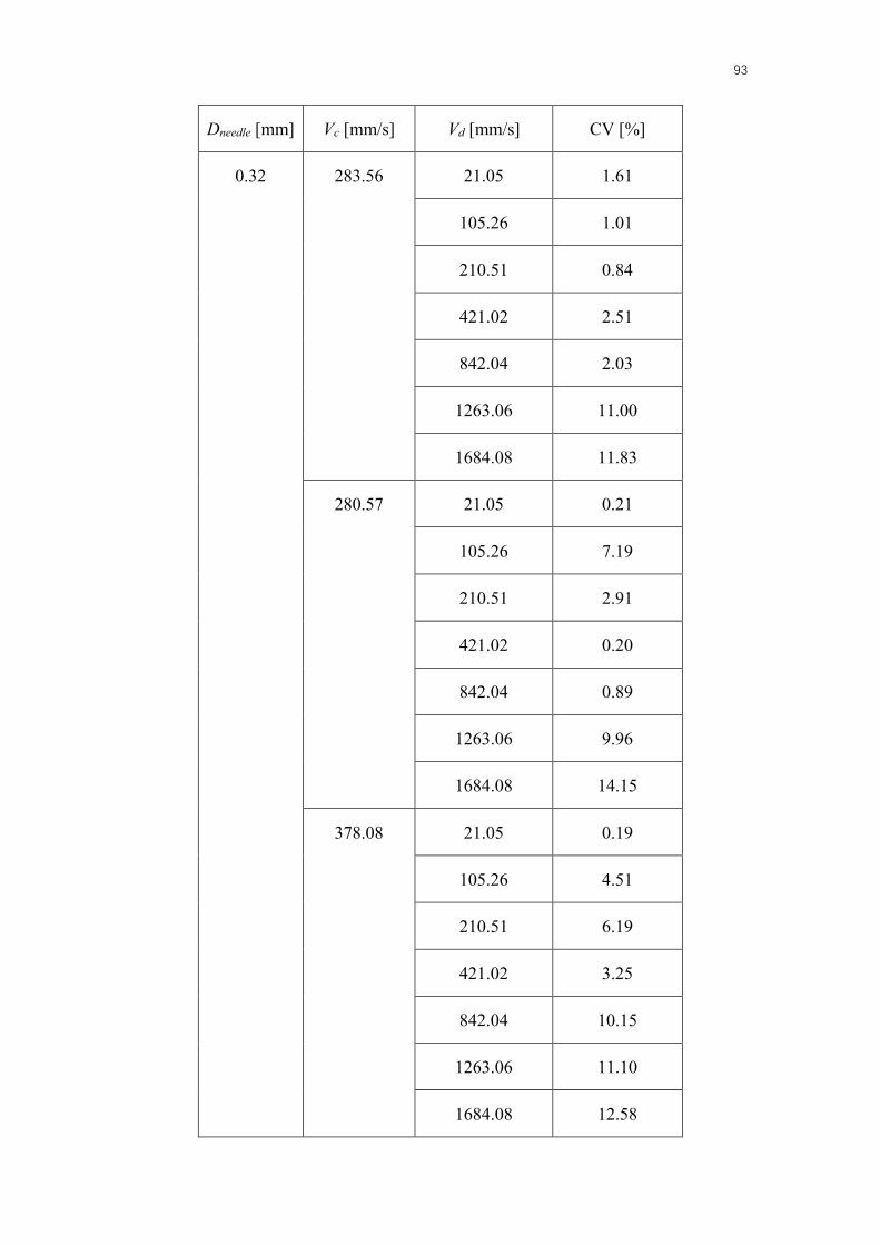
93
Dneedle [mm] Vc [mm/s] Vd [mm/s] CV [%]
0.32 283.56 21.05 1.61
105.26 1.01
210.51 0.84
421.02 2.51
842.04 2.03
1263.06 11.00
1684.08 11.83
280.57 21.05 0.21
105.26 7.19
210.51 2.91
421.02 0.20
842.04 0.89
1263.06 9.96
1684.08 14.15
378.08 21.05 0.19
105.26 4.51
210.51 6.19
421.02 3.25
842.04 10.15
1263.06 11.10
1684.08 12.58

94
Appendix C. The Calculation of Dimensionless Parameters
Table C-1. The parameters of the nondimensional analysis.
Dneedle [mm] Vc [mm/s] Vd [mm/s] Vd/Vc Ddrop/Dneedle
0.14 140.28 108.73 0.77 4.47
543.67 3.86 5.70
1087.34 7.72 6.40
2174.68 15.43 5.24
189.04 108.73 0.57 3.92
543.67 2.86 5.09
1087.34 5.73 5.41
2174.68 11.46 4.71
210.42 108.73 0.51 3.67
543.67 2.57 4.70
1087.34 5.15 4.90
2174.68 10.29 4.55
(Continued)
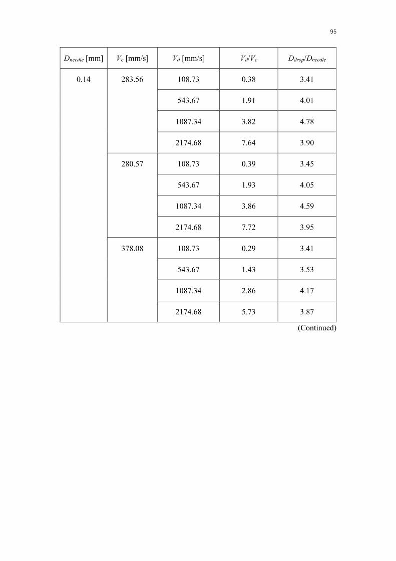
95
Dneedle [mm] Vc [mm/s] Vd [mm/s] Vd/Vc Ddrop/Dneedle
0.14 283.56 108.73 0.38 3.41
543.67 1.91 4.01
1087.34 3.82 4.78
2174.68 7.64 3.90
280.57 108.73 0.39 3.45
543.67 1.93 4.05
1087.34 3.86 4.59
2174.68 7.72 3.95
378.08 108.73 0.29 3.41
543.67 1.43 3.53
1087.34 2.86 4.17
2174.68 5.73 3.87
(Continued)

96
Dneedle [mm] Vc [mm/s] Vd [mm/s] Vd/Vc Ddrop/Dneedle
0.32 140.28 105.26 0.74 5.79
210.51 1.48 6.30
421.02 2.95 6.67
842.04 5.91 6.84
1263.06 8.86 4.86
1684.08 11.82 5.19
189.04 105.26 0.55 5.07
210.51 1.10 5.39
421.02 2.19 5.71
842.04 4.39 6.50
1263.06 6.58 4.38
1684.08 8.77 4.62
210.42 21.05 0.10 3.50
105.26 0.49 4.30
210.51 0.98 4.78
421.02 1.97 5.02
842.04 3.94 5.78
1263.06 5.91 3.88
1684.08 7.88 4.33
(Continued)

97
Dneedle [mm] Vc [mm/s] Vd [mm/s] Vd/Vc Ddrop/Dneedle
0.32 283.56 21.05 0.07 2.78
105.26 0.37 3.35
210.51 0.73 3.74
421.02 1.46 4.06
842.04 2.92 5.45
1263.06 4.38 3.48
1684.08 5.85 3.82
280.57 21.05 0.07 2.84
105.26 0.37 3.36
210.51 0.74 3.67
421.02 1.48 4.00
842.04 2.95 5.16
1263.06 4.43 3.50
1684.08 5.91 3.71
378.08 21.05 0.05 2.67
105.26 0.27 3.09
210.51 0.55 3.29
421.02 1.10 3.59
842.04 2.19 5.07
1263.06 3.29 3.40
1684.08 4.38 3.47

98
Appendix D. The Calculation of Nondimensional Numbers
Table D-1. The calculations of the nondimensional numbers (Ca and We).
Dneedle [mm] Vc [mm/s] Vd [mm/s] Ca We
0.14 140.28 108.73 59.2 0.036706657
543.67 0.917733957
1087.34 3.670935828
2174.68 14.68374331
189.04 108.73 79.8
0.036706657
543.67 0.917733957
1087.34 3.670935828
2174.68 14.68374331
210.42 108.73 88.8 0.036706657
543.67 0.917733957
1087.34 3.670935828
2174.68 14.68374331
(Continued)
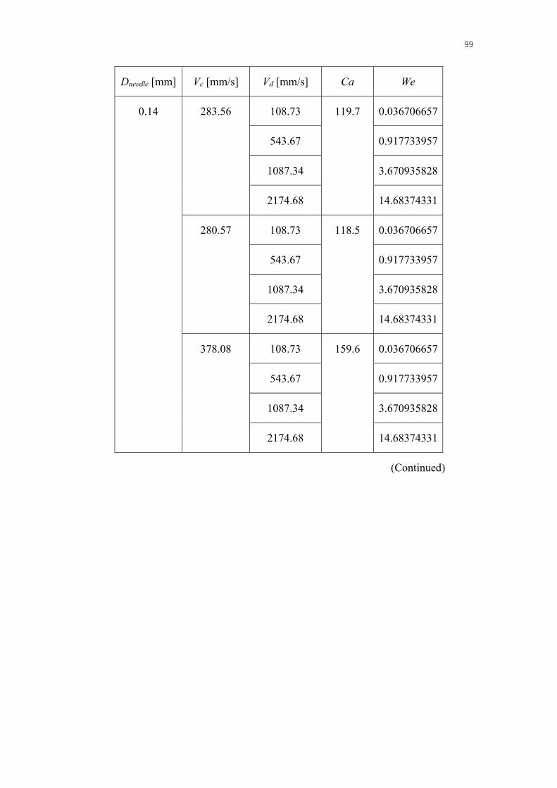
99
Dneedle [mm] Vc [mm/s] Vd [mm/s] Ca We
0.14 283.56 108.73 119.7 0.036706657
543.67 0.917733957
1087.34 3.670935828
2174.68 14.68374331
280.57 108.73 118.5 0.036706657
543.67 0.917733957
1087.34 3.670935828
2174.68 14.68374331
378.08 108.73 159.6 0.036706657
543.67 0.917733957
1087.34 3.670935828
2174.68 14.68374331
(Continued)

100
Dneedle [mm] Vc [mm/s] Vd [mm/s] Ca We
0.32 140.28 105.26 59.2 0.07863117
210.51 0.3144948
421.02 1.257979198
842.04 5.031916792
1263.06 11.32181278
1684.08 20.12766717
189.04 105.26 79.8 0.07863117
210.51 0.3144948
421.02 1.257979198
842.04 5.031916792
1263.06 11.32181278
1684.08 20.12766717
210.42 21.05 88.8 0.003144649
105.26 0.07863117
210.51 0.3144948
421.02 1.257979198
842.04 5.031916792
1263.06 11.32181278
1684.08 20.12766717
(Continued)

101
Dneedle [mm] Vc [mm/s] Vd [mm/s] Ca We
0.32 283.56 21.05 119.7 0.003144649
105.26 0.07863117
210.51 0.3144948
421.02 1.257979198
842.04 5.031916792
1263.06 11.32181278
1684.08 20.12766717
280.57 21.05 118.5 0.003144649
105.26 0.07863117
210.51 0.3144948
421.02 1.257979198
842.04 5.031916792
1263.06 11.32181278
1684.08 20.12766717
378.08 21.05 159.6 0.003144649
105.26 0.07863117
210.51 0.3144948
421.02 1.257979198
842.04 5.031916792
1263.06 11.32181278
1684.08 20.12766717

102
Table D-2. The calculations of the nondimensional numbers (OhCP and Ca/OhCP).
Dneedle [mm] Vc [mm/s] Vd [mm/s] OhCP Ca/OhCP
0.14 140.28 108.73 0.258127 0.229458
543.67
1087.34
2174.68
189.04 108.73 0.309215
543.67
1087.34
2174.68
210.42 108.73 0.344187
543.67
1087.34
2174.68
(Continued)

103
Dneedle [mm] Vc [mm/s] Vd [mm/s] OhCP Ca/OhCP
0.14 283.56 108.73 0.258127 0.463823
543.67
1087.34
2174.68
280.57 108.73 0.458932
543.67
1087.34
2174.68
378.08 108.73 0.618430
543.67
1087.34
2174.68
(Continued)

104
Dneedle [mm] Vc [mm/s] Vd [mm/s] OhCP Ca/OhCP
0.32 140.28 105.26 0.170735 0.346908
210.51
421.02
842.04
1263.06
1684.08
189.04 105.26 0.467489
210.51
421.02
842.04
1263.06
1684.08
210.42 21.05 0.520361
105.26
210.51
421.02
842.04
1263.06
1684.08
(Continued)

105
Dneedle [mm] Vc [mm/s] Vd [mm/s] OhCP Ca/OhCP
0.32 283.56 21.05 0.170735 0.701234
105.26
210.51
421.02
842.04
1263.06
1684.08
280.57 21.05 0.693840
105.26
210.51
421.02
842.04
1263.06
1684.08
378.08 21.05 0.934979
105.26
210.51
421.02
842.04
1263.06
1684.08

106
Appendix E. The Calculation of Torque Balance Equation
Table E-1. The calculations of Ddrop using TBE.
Dneedle [mm] Vc [mm/s] Vd [mm/s] Ddrop [μm]
0.14 140.28 108.73 898.7
543.67
1087.34
2174.68
189.04 108.73 729.3
543.67
1087.34
2174.68
210.42 108.73 675.5
543.67
1087.34
2174.68
(Continued)

107
Dneedle [mm] Vc [mm/s] Vd [mm/s] Ddrop [μm]
0.14 283.56 108.73 542.7
543.67
1087.34
2174.68
280.57 108.73 547.0
543.67
1087.34
2174.68
378.08 108.73 435.3
543.67
1087.34
2174.68
(Continued)

108
Dneedle [mm] Vc [mm/s] Vd [mm/s] Ddrop [μm]
0.32 140.28 105.26 1503.9
210.51
421.02
842.04
1263.06
1684.08
189.04 105.26 1218.6
210.51
421.02
842.04
1263.06
1684.08
210.42 21.05 1126.2
105.26
210.51
421.02
842.04
1263.06
1684.08
(Continued)

109
Dneedle [mm] Vc [mm/s] Vd [mm/s] Ddrop [μm]
0.32 283.56 21.05 894.5
105.26
210.51
421.02
842.04
1263.06
1684.08
280.57 21.05 902.2
105.26
210.51
421.02
842.04
1263.06
1684.08
378.08 21.05 699.9
105.26
210.51
421.02
842.04
1263.06
1684.08

110
References
1. R. Seemann, M.B., T. Pfohl and S. Herminghaus, Droplet Based Microfluidics. Rep. Prog.
Phys., 2011. 75(1): p. 016601.
2. Wang, P.Z.a.L., Passive and Active Droplet Generation with Microfluidics: A Review. Lab
Chip, 2017. 17(1): p. 34-75.
3. Schramm, L.L., Emulsions, Foams, and Suspensions: Fundamentals and Applications2006:
John Wiley & Sons.
4. Anna, G.F.C.a.S.L., Microfluidic Methods for Generating Continuous Droplet Streams. J. Phys. D, 2007. 40(19): p. R319.
5. S. Y. Teh, R.L., L. H. Hung and A. P. Lee, Droplet Microfluidics. Lab Chip, 2008. 8(2): p. 198-
220.
6. M. Abkarian, E.L., and G. Massiera, Continuous Droplet Interface Crossing Encapsulation (cDICE) for High Throughput Monodisperse Vesicle Design. Soft Matter, 2011. 7(10): p.
4610-4614.
7. A. Rakszewska, J.T., V. Chokkalingam and W. T. S. Huck, One Drop at A Time: Toward Droplet Microfluidics as A Versatile Tool for Single-cell Analysis. NPG Asia Mater., 2014.
6: p. e133.
8. J. F. Edd, D.D.C., K. J. Humphry, S. Köster, D. Irimia, D. A. Weitz and M. Toner, Controlled Encapsulation of Single-cells into Monodisperse Picolitre Drops. Lab Chip, 2008. 8(8): p.
1262-1264.
9. Trägårdh, S.M.J.a.G., Membrane Emulsification—A Literature Review. J. Membr. Sci. , 2000.
169(1): p. 107-117.
10. V. Trivedi, A.D., G. K. Kurup, E. Ereifej, P. J. Vandevord and A. S. Basu, A Modular Approach for the Generation, Storage, Mixing, and Detection of Droplet Libraries for High Throughput Screening. Lab Chip, 2010. 10(18): p. 2433-2442.
11. I. Ziemecka, V.v.S., G. J. M. Koper, M. Rosso, A. M. Brizard, J. H. van Esch and M. T. Kreutzer,
Monodisperse Hydrogel Microspheres by Forced Droplet Formation in Aqueous Two-phase Systems. Lab Chip, 2011. 11(4): p. 620-624.
12. R. Ito, Y.H., K. Inoue and Y. Kitagawa, Formation of Liquid Drop through a Nozzle in Uniform Stream. Kagaku Kougaku Ronbunshu 1979. 5(3): p. 288-292.
13. Williams, S.J.P.a.R.A., Controlled Production of Emulsions Using a Crossflow Membrane: Part I: Droplet Formation from a Single Pore. Chem. Eng. Res. Des. , 1998. 76(8): p. 894-
901.
14. Peng, S.J. and R.A. Williams, Controlled Production of Emulsions Using a Crossflow Membrane: Part I: Droplet Formation from a Single Pore. Chemical Engineering Research
and Design, 1998. 76(8): p. 894-901.
15. R. A. Williams, S.J.P., D. A. Wheeler, N. C. Morley, D. Taylor, M. Whalley and D. W.
Houldsworth, Controlled Production of Emulsions Using a Crossflow Membrane: Part II: Industrial Scale Manufacture. Chem. Eng. Res. Des. , 1998. 76(8): p. 902-910.
16. A. J. Gijsbertsen-Abrahamse, A.v.d.P.a.R.M.B., Status of Cross-flow Membrane Emulsification and Outlook for Industrial Application. J. Membr. Sci. , 2004. 230(1-2): p.
149-159.

111
17. I. Kobayashi, M.N., K. Chun, Y. Kikuchi and H. Fujita, Silicon Array of Elongated through-holes for Monodisperse Emulsion Droplets. AIChE J., 2002. 48(8): p. 1639-1644.
18. T. Nisisako, T.T.a.T.H., Droplet Formation in a Microchannel Network. Lab Chip, 2002. 2(1):
p. 24-26.
19. Pit, A., M. Duits, and F. Mugele, Droplet manipulations in two phase flow microfluidics. Micromachines, 2015. 6(11): p. 1768-1793.
20. Anna, S.L., Droplets and Bubbles in Microfluidic Devices. Annu. Rev. Fluid Mech., 2016. 48:
p. 285-309.
21. Crocker, R.F.M.a.J.C., Universal Dripping and Jetting in a Transverse Shear Flow. Phys. Rev.
Lett., 2009. 102(19): p. 194501.
22. A. J. Abrahamse, R.v.L., R. G. M. van der Sman, A. van der Padt and R. M. Boom, Analysis of Droplet Formation and Interactions During Cross-flow Membrane Emulsification. J.
Membr. Sci. , 2002. 204(1-2): p. 125-137.
23. J. Zawala, K.S.a.P.W., Theoretical and Experimental Studies of Drop Size in Membrane Emulsification–Single Pore Studies of Hydrodynamic Detachment of Droplets. Colloids
Surf. A, 2015. 470: p. 297-305.
24. D. X. Hao, F.L.G., G. H. Hu, Y. J. Zhao, G. P. Lian, G. H. Ma and Z. G. Su, Controlling Factors on Droplets Uniformity in Membrane Emulsification: Experiment and Modeling Analysis. Ind. Eng. Chem. Res., 2008. 47(17): p. 6418-6425.
25. N. C. Christov, K.D.D., D. K. Danova and P. A. Kralchevsky, The Drop Size in Membrane Emulsification Determined From the Balance of Capillary and Hydrodynamic Forces. Langmuir, 2008. 24(4): p. 1397-1410.
26. G. De Luca, A.D.R., F. P. Di Maio and E. Drioli, Modelling Droplet Formation in Cross-flow Membrane Emulsification. Desalination, 2006. 199(1-3): p. 177-179.
27. M. J. Geerken, R.G.H.L.a.M.W., Interfacial Aspects of Water Drop Formation at Micro-engineered Orifices. J. Colloid Interface Sci. , 2007. 312(2): p. 460-469.
28. A. Timgren, G.T.a.C.T., A Model for Drop Size Prediction during Cross-flow Emulsification. Chem. Eng. Res. Des., 2010. 88(2): p. 229-238.
29. Trägårdh, M.R.a.G., Membrane Emulsification Modelling: How can We Get from Characterisation to Design? Desalination, 2002. 145(1-3): p. 165-172.
30. K. Feigl, F.X.T., S. Holzapfel and E. J. Windhab, Effect of Flow Type, Channel Height, and Viscosity on Drop Production from Micro-pores. Chem. Eng. Sci., 2014. 116: p. 372-382.
31. Z. Wang, S.C.W., V. Schroeder and H. Schubert, Influence of Fluid Flow on Forces Acting on Droplet and Emulsification Results in Membrane Emulsification Process. Chin. J. Chem.
Eng. , 1999. 50(4): p. 505-513.
32. A. M. Pit, M.H.G.D.a.F.M., Droplet Manipulations in Two Phase Flow Microfluidics. Micromachines, 2015. 6(11): p. 1768-1793.
33. T. Thorsen, R.W.R., F. H. Arnold and S. R. Quake, Depletion Interactions and Fractionated Crystallization for Polydisperse Emulsion Purification Phys. Rev. Lett, 2001. 86: p. 4163-
4166.
34. P. Garstecki, I.G., W. DiLuzio, G. M. Whitesides, E. Kumacheva and H. A. Stone, Formation of Monodisperse Bubbles in a Microfluidic Flow-focusing Device. Appl. Phys. Lett., 2004.
85(13): p. 2649-2651.
35. B. Zheng, J.D.T.a.R.F.I., Formation of Droplets of Alternating Composition in Microfluidic
112
Channels and Applications to Indexing of Concentrations in Droplet-based Assays. Anal.
Chem. , 2004. 76(17): p. 4977-4982.
36. P. Garstecki, M.J.F., H. A. Stone and G. M. Whitesides, Formation of Droplets and Bubbles in a Microfluidic T-junction—Scaling and Mechanism of Break-up. Lab Chip, 2006. 6(3):
p. 437-446.
37. Zhang, H.H.L.a.Y.H., Droplet Formation in a T-shaped Microfluidic Junction. J. Appl. Phys.,
2009. 106(3): p. 034906.
38. A. Bertrandias, H.D., J. Casalinho and M. L. Giorgi, Dripping to Jetting Transition for Cross-flowing Liquids. Phys. Fluids, 2017. 29(4): p. 044102.
39. É. Lepercq-Bost, M.L.G., A. Isambert and C. Arnaud, Use of the Capillary Number for the Prediction of Droplet Size in Membrane Emulsification. J. Membr. Sci. , 2008. 314(1-2): p.
76-89.
40. S. Zhang, C.G.-C., S. Veesler and N. Candoni, Prediction of Sizes and Frequencies of Nanoliter-sized Droplets in Cylindrical T-junction Microfluidics. Chem. Eng. Sci., 2015. 138:
p. 128-139.
41. A. S. Utada, L.Y.C., A. Fernandez-Nieves, D. R. Link, C. Holtze and D. A. Weitz, Dripping, Jetting, Drops, and Wetting: The Magic of Microfluidics. MRS Bull., 2007. 32(9): p. 702-
708.
42. Pathak, M., Numerical Simulation of Membrane Emulsification: Effect of Flow Properties in the Transition from Dripping to Jetting. J. Membr. Sci. , 2011. 382(1-2): p. 166-176.
43. G. De Luca, F.P.D.M., A. Di Renzo and E. Drioli, Droplet Detachment in Cross-flow Membrane Emulsification: Comparison among Torque-and Force-based Models. Chem.
Eng. Process., 2008. 47(7): p. 1150-1158.
44. Wang, Z.W.a.S.C., Effect of Continuous Phase Viscosity on Membrane Emulsification. Chin.
J. Chem. Eng. , 2000. 8(2): p. 108-112.
45. G. De Luca, A.S., L. Giorno and E. Drioli, Quantitative Analysis of Coupling Effects in Cross-flow Membrane Emulsification. J. Membr. Sci. , 2004. 229(1-2): p. 199-209.
46. A. Timgren, G.T.a.C.T., Application of the PIV Technique to Measurements around and inside a Forming Drop in a Liquid–liquid System. Exp. Fluids, 2008. 44(4): p. 565-575.
47. Pathak, M., Numerical Simulation of Droplet Dynamics in Membrane Emulsification Systems, in Numerical Simulation-From Theory to Industry2012, InTech.
48. Ulbrecht, Y.K.a.J.J., Formation of Drops and Bubbles in Flowing Liquids. Ind. Eng. Chem.
Process Des. Dev., 1981. 20(4): p. 636-640.
49. V. Schröder, O.B.a.H.S., Effect of Dynamic Interfacial Tension on the Emulsification Process Using Microporous, Ceramic Membranes. J. Colloid Interface Sci. , 1998. 202(2): p. 334-
340.
50. M. Rayner, G.T., C. Trägårdh and P. Dejmek, Using the Surface Evolver to Model Droplet Formation Processes in Membrane Emulsification. J. Colloid Interface Sci. , 2004. 279(1):
p. 175-185.
51. J. H. Xu, G.S.L., G. G. Chen and J. D. Wang, Experimental and Theoretical Approaches on Droplet Formation from a Micrometer Screen Hole. J. Membr. Sci. , 2005. 266(1-2): p.
121-131.
52. O. E. Yildirim, Q.X.a.O.A.B., Analysis of the Drop Weight Method. Phys. Fluids, 2005. 17(6):
p. 062107.

113
53. Tolman, R.C., The Effect of Droplet Size on Surface Tension. J. Chem. Phys., 1949. 17(3): p.
333-337.
54. Demarquette, E.Y.A.a.N.R., Use of the Pendant Drop Method to Measure Interfacial Tension Between Molten Polymers. Mater. Res., 1999. 2(1): p. 23-32.
55. B. B. Lee, P.R.a.E.S.C., New Drop Weight Analysis for Surface Tension Determination of Liquids. Colloids Surf. A, 2009. 332(2-3): p. 112-120.
56. M. D. Abràmoff, P.J.M.a.S.J.R., Image Processing with ImageJ. Biophotonics international.
Vol. 11. 2004. 36-42.
57. C. A. Schneider, W.S.R.a.K.W.E., NIH Image to ImageJ: 25 years of Image Analysis. Nat.
Methods, 2012. 9(7): p. 671.
58. Z. Z. Chong, S.B.T., A. M. Gañán-Calvo, Z. J. Chong, N. H. Loh, N. T. Nguyen and S. H. Tan,
Automated Droplet Measurement (ADM): An Enhanced Video Processing Software for Rapid Droplet Measurements. Microfluid. Nanofluid., 2016. 20(4): p. 66.
59. Z. Z. Chong, S.H.T., A. M. Gañán-Calvo, S. B. Tor, N. H. Loh and N. T. Nguyen, Active Droplet Generation in Microfluidics. Lab Chip, 2016. 16(1): p. 35-58.
60. R. F. Meyer, W.B.R., M. T. McClendon and J. C. Crocker, Producing Monodisperse Drug-loaded Polymer Microspheres via Cross-flow Membrane Emulsification: The Effects of Polymers and Surfactants. Langmuir, 2010. 26(18): p. 14479-14487.
61. J. H. Xu, S.W.L., J. Tan, Y. J. Wang and G. S. Luo, Preparation of Highly Monodisperse Droplet in a T-junction Microfluidic Device. AIChE Journal, 2006. 52(9): p. 3005-3010.
62. F. Malloggi, N.P., R. Attia, F. Monti, P. Mary, H. Willaime, P. Tabeling, B. Cabane and P.
Poncet, Monodisperse Colloids Synthesized with Nanofluidic Technology. Langmuir, 2009.
26(4): p. 2369-2373.
63. G. T. Vladisavljevic, I.K.a.M.N., Production of Uniform Droplets Using Membrane, Microchannel and Microfluidic Emulsification Devices. Microfluid. Nanofluid., 2012. 13(1):
p. 151-178.
64. M. M. Dragosavac, G.T.V., R. G. Holdich and M. T. Stillwell, Production of Porous Silica Microparticles by Membrane Emulsification. Langmuir, 2011. 28(1): p. 134-143.
65. L. Y. Chu, A.S.U., R. K. Shah, J. W. Kim and D. A. Weitz, Controllable Monodisperse Multiple Emulsions. Angew. Chem., 2007. 119(47): p. 9128-9132.
66. D. Saeki, S.S., T. Kanamori, S. Sato and S. Ichikawa, Formation of Monodisperse Calcium Alginate Microbeads by Rupture of Water-in-oil-in-water Droplets with an Ultra-thin Oil Phase Layer. Lab Chip, 2010. 10(17): p. 2292-2295.