drainage criteria and design manual san patricio county, texas · san patricio county, texas ......
TRANSCRIPT

DRAINAGE CRITERIA AND DESIGN MANUAL
SAN PATRICIO COUNTY, TEXAS
SAN PATRICIO COUNTY DRAINAGE DISTRICT
JULY '1987
v
~ HDR Inf,a.I,uclu,." IIlC, A Centerra Compa"y
t"'IBUITH etlGlNE~n8. mc. Con.ultlnn EngIne era

DRAINAGE CRITERIA
and DESIGN MANUAL
SAN PATRICIO COUNTY, TEXAS
SAN PATRICIO COUNTY DRAINAGE DISTRICT
July, 1987
Prepared by
HDR Infrastructure, Inc. Austin, Texas
Naismith Engineers, Inc. Corpus Christi, Texas

TABLE OF CONTENTS
SECTION
1 - I NTRODUCTI ON
1.10 Purpose 1.20 Objectives 1.30 Planning Requirements
1.31 Coordination of Planning Efforts 1.40 Design Requirements
1.41 Design Storm Frequencies 1.42 Initial Storm Provisions 1.43 Major Storm Provisions 1.44 Hydrologic Analysis 1.45 Maximum Permissible Flooding 1.46 Channels
1.50 Coordination With Flood Control Study and Profiles
1.60 Plan Submittal Standards
2 - STORM RUNOFF
2.10 General 2.20 Rational Method
2.21 Runoff Coefficient, C 2.21.1 Nature of Surface 2.21.2 Soil
Maps
2.21.3 Using the Runoff Co~fficient 2.22 Rainfall Intensity, i 2.23 Time of Concentration
2.23.1 Overland Flow 2.23.2 Storm Sewer or Road
Gutter Flow 2.23.3 Channel Flow
2.30 Regional Flood Analysis
3 - STREET FLOW
PAGE
1-1 1-1
1-2 1-2 1-3 1-3 1-3 1-3 1-3 1-4 1-4
1-5
2-1 2-1 2-2 2-2 2-3 2-3 2-4 2-4 2-8 2-8
2-8 2-11
3.10 General 3-1 3.20 Effects of Stormwater on Street Capacity 3-1
3.21 Interference Due to Sheet Flow Across Pavement 3-1 3.21.1 Hydroplaning 3-2 3.21.2 Splash 3-2
3.22 Interference Due to Gutter Flow 3-2 3.23 Interference Due to Ponding 3-3 3.24 Interference Due to Water Flowing Across 3-3
Traffic Lane 3.25 Effect on Pedestrians 3-4
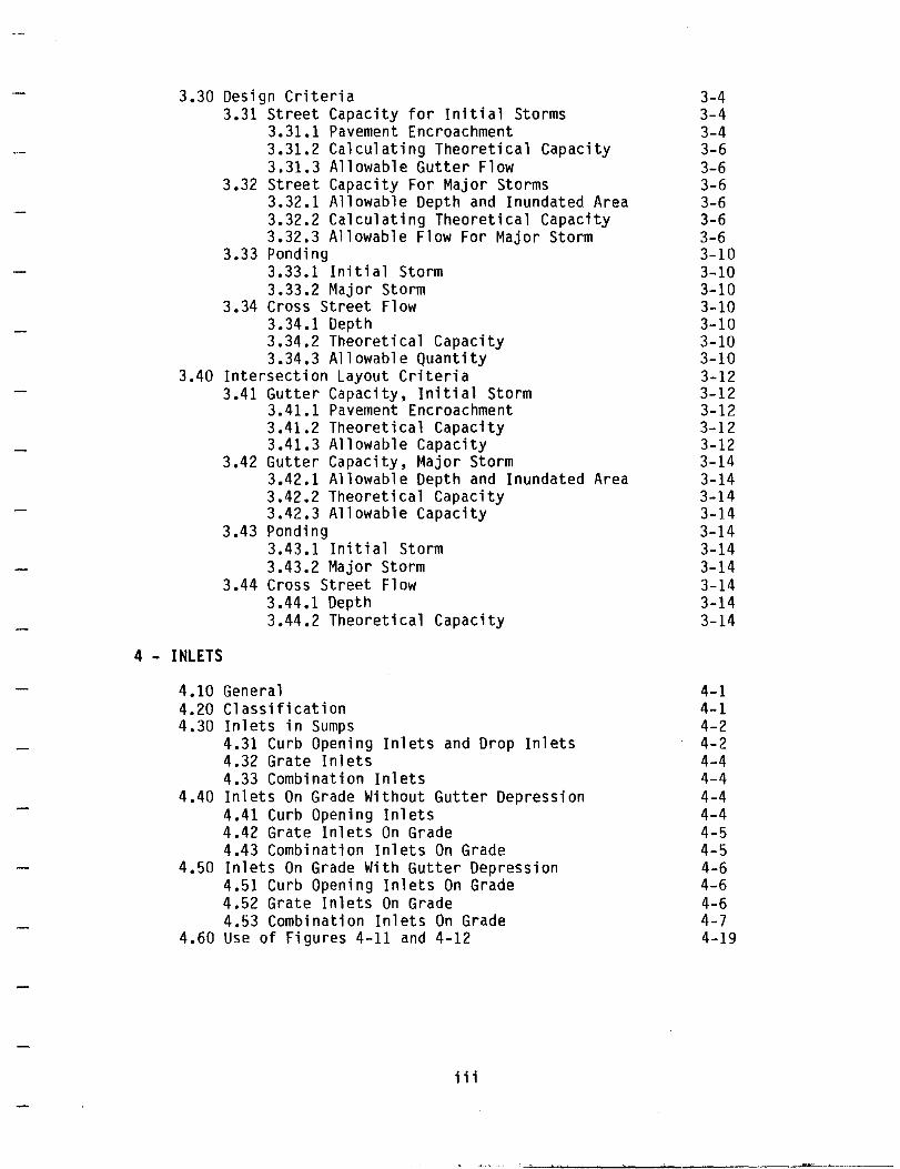
3.30 Design Criteria 3-4 3.31 Street Capacity for Initial Storms 3-4
3.31.1 Pavement Encroachment 3-4 3.31.2 Calculating Theoretical Capacity 3-6 3.31.3 Allowable Gutter Flow 3-6
3.32 Street Capacity For Major Storms 3-6 3.32.1 Allowable Depth and Inundated Area 3-6 3.32.2 Calculating Theoretical Capacity 3-6 3.32.3 Allowable Flow For Major Storm 3-6
3.33 Ponding 3-10 3.33.1 Initial Storm 3-10 3.33.2 Major Storm 3-10
3.34 Cross Street Flow 3-10 3.34.1 Depth 3-10 3.34.2 Theoretical Capacity 3-10 3.34.3 Allowable Quantity 3-10
3.40 Intersection Layout Criteria 3-12 3.41 Gutter Capacity, Initial Storm 3-12
3.41.1 Pavement Encroachment 3-12 3.41.2 Theoretical Capacity 3-12 3.41.3 Allowable Capacity 3-12
3.42 Gutter Capacity, Major Storm 3-14 3.42.1 Allowable Depth and Inundated Area 3-14 3.42.2 Theoretical Capacity 3-14 3.42.3 Allowable Capacity 3-14
3.43 Ponding 3-14 3.43.1 Initial Storm 3-14 3.43.2 Major Storm 3-14
3.44 Cross Street Flow 3-14 3.44.1 Depth 3-14 3.44.2 Theoretical Capacity 3-14
4 - INLETS
4.10 General 4-1 4-1 4-2 4-2 4-4 4-4 4-4 4-4 4-5 4-5 4-6 4-6 4-6 4-7 4-19
4.20 Classification 4.30 Inlets in Sumps
4.31 Curb Opening Inlets and Drop Inlets 4.32 Grate Inlets 4.33 Combination Inlets
4.40 Inlets On Grade Without Gutter Depression 4.41 Curb Opening Inlets 4.42 Grate Inlets On Grade 4.43 Combination Inlets On Grade
4.50 Inlets On Grade With Gutter Depression 4.51 Curb Opening Inlets On Grade 4.52 Grate Inlets On Grade 4.53 Combination Inlets On Grade
4.60 Use of Figures 4-11 and 4-12
iii
.~~~-......... - ........ ----~--~~--.. ----

5 - STORM DRAINS
5.10 General 5-1 5.20 Velocities and Grades 5-1
5.21 Minimum Grades 5-1 5.22 Maximum Velocities 5-1 5.23 Minimum Diameter 5-1
5.30 Materials 5-4 5.40 Full or Part Full Flow In Storm Drains 5-4
5.41 General 5-4 5.42 Pipe Flow Charts 5-5
5.50 Hydraulic Gradient and Profile of Storm Drain 5-5 5.60 Manhole Locations 5-6 5.70 Pipe Connections 5-6 5.80 Minor Head Losses at Structures 5-7 5.90 Utilities 5-11
6 - OPEN CHANNEL FLOW
6.10 General 6.20 Channel Discharge
6.21 Manning's Equation 6.22 Uniform Flow 6.23 Normal Depth
6.30 Design Considerations 6.40 Channel Cross Sections
6.41 Side Slope 6.42 Depth 6.43 Bottom Width 6.44 Trickle Channels 6.45 Freeboard
6.50 Channel Drops 6.60 Supercritical Flow
7 - CULVERT DESIGN
7.10 General 7.20 Design Criteria
7.21 Design Frequency 7.22 Culvert Discharge Velocities
7.30 Cul vert Types 7.31 Mild Slope Regime, Critical Depth
(Outlet Control) Control
7.32 Mild Slope Regime, Tailwater Depth Control (Outlet Control)
7.33 Steep Slope Regime, Tailwater Insignificant (Entrance Control)
7.34 "Slug" Flow Operation (Outlet/Entrance Control)
7.35 Mild Slope Regime, Tailwater Greater Than Barrel Depth (Outlet Control)
7.36 Mild Slope Regime, Tailwater Less Than Barrel Depth (Outlet Control)
iv
~~~-"~~
6-1 6-1 6-1 6-2 6-2 6-5 6-5 6-3 6-3 6-10 6-10 6-10 6-11 6-11
7-1 7-1 7-1 7-1 7-2 7-2
7-5
7-6
7-7
7-8
7-9

7.40 End Treatments 7.41 Conditions at Entrance 7.42 Parallel Headwall and Endwall 7.43 Flared Headwall and Endwall 7.44 Warped Headwall and Endwall 7.45 Improved Inlets
7.50 Culvert Design With Standard Inlets 7.51 Culvert Sizing 7.52 Use of Nomographs
7.60 Design Procedure 7.61 Design Computation Forms 7.62 Invert Elevations 7.63 Culvert Diameters 7.64 Limited Headwater
8 - BRIDGES
8.10 General 8.20 Terminology 8.30 Flow Through Bridges 8.40 Single Structure 8.50 Multiple Structures
8.51 Flow Distribution 8.52 Design of Multiple Structures
8.60 Spur Dikes
REFERENCES
v
7-10 7-10 7-13 7-13 7-13 7-13 7-13 7-14 7-14 7-15 7-15 7-15 7-15 7-16
8-1 8-1 8-2 8-5 8-6 8-6 8-8 8-10
R-l

Table
2-1
2-2
3-1 3-2 3-3
5-1
5-2 5-3 5-4 5-5 5-6
6-1 6-2
7-1 7-2
LIST OF TABLES
Rational Method Runoff Coefficients by Land Use Types
Rational Method Runoff Coefficients for Composite Analysis
Allowable Initial Storm Runoff Encroachment Allowable Major Storm Runoff Inundation Allowable Cross Street Flow
Minimum Slope Required to Produce Scouring Velocity
Maximum Velocity in Storm Drains Roughness Coefficients "n" for Storm Drains Junctiori or Structure Coefficient of Loss Head Loss Coefficients Due to Obstructions Head Loss Coefficients Due to Sudden
Enlargements and Contractions
Composite Roughness Coefficient "n" for Channels Roughness Coefficient On" for Channels
Culvert Discharge Velocity Limitations Culvert Entrance Loss Coefficients
vi
2-3
2-5
3-5 3-7 3-11
5-2
5-3 5-3 5-8 5-9 5-10
6-6 6-7
7-2 7-4
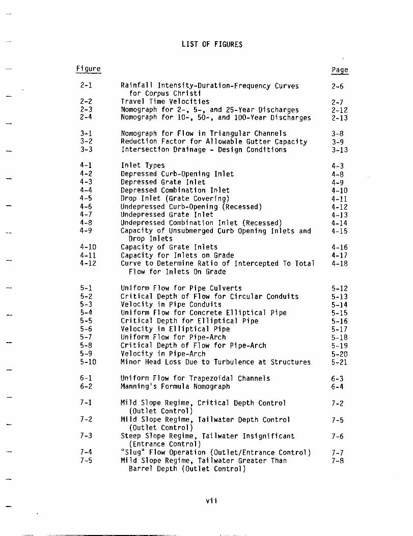
Figure
2-1
2-2 2-3 2-4
3-1 3-2 3-3
4-1 4-2 4-3 4-4 4-5 4-6 4-7 4-8 4-9
4-10 4-11 4-12
5-1 5-2 5-3 5-4 5-5 5-6 5-7 5-8 5-9 5-10
6-1 6-2
7-1
7-2
7-3
7-4 7-5
LIST OF FIGURES
Rainfall Intensity-Duration-Frequency Curves for Corpus Christi
Travel Time Velocities Nomograph for 2-, 5-, and 25-Year Discharges Nomograph for 10-, 50-, and 100-Year Discharges
Nomograph for Flow in Triangular Channels Reduction Factor for Allowable Gutter Capacity Intersection Drainage - Design Conditions
Inlet Types Depressed Curb-Opening Inlet Depressed Grate Inlet Depressed Combination Inlet Drop Inlet (Grate Covering) Undepressed Curb-Opening (Recessed) Undepressed Grate Inlet Undepressed Combination Inlet (Recessed) Capacity of Unsubmerged Curb Opening Inlets and
Drop Inlets Capacity of Grate Inlets Capacity for Inlets on Grade Curve to Determine Ratio of Intercepted To Total
Flow for Inlets On Grade
Uniform Flow for Pipe Culverts Critical Depth of Flow for Circular Conduits Velocity in Pipe Conduits Uniform Flow for Concrete Elliptical Pipe Critical Depth for Elliptical Pipe Velocity in Elliptical Pipe Uniform Flow for Pipe-Arch Critical Depth of Flow for Pipe-Arch Velocity in Pipe-Arch Minor Head Loss Due to Turbulence at Structures
Uniform Flow for Trapezoidal Channels Manning's Formula Nomograph
Mild Slope Regime, Critical Depth Control (Outlet Control)
Mild Slope Regime, Tailwater Depth Control (Outlet Control)
Steep Slope Regime, Tailwater Insignificant (Entrance Control)
"Slug" Flow Operation (Outlet/Entrance Control) Mild Slope Regime, Tailwater Greater Than
Barrel Depth (Outlet Control)
vii
Page
2-6
2-7 2-12 2-13
3-8 3-9 3-13
4-3 4-8 4-9 4-10 4-11 4-12 4-13 4-14 4-15
4-16 4-17 4-18
5-12 5-13 5-14 5-15 5-16 5-17 5-18 5-19 5-20 5-21
6-3 6-4
7-2
7-5
7-6
7-7 7-8

7-6
7-7 7-8 7-9
7-10
7-11
7-12
7-13
7-14
7-15
8-1 8-2 8-3 8-4 8-5
Mild Slope Regime, Tailwater Less Than Barrel Depth (Outlet Control)
Critical Depth of Flow for Circular Conduits Critical Flow for Box Culverts Outlet Control Nomograph - Head for Concrete Box
Culverts Flowing Full, n = 0.012 Inlet Control Nomograph - Headwater Depth for Box
Culverts with Inlet Control Outlet Control Nomograph - Head for Concrete Pipe
Culvert Flowing Full, n = 0.012 Outlet Control Nomograph - Head for Standard
C.M. Pipe Culverts Flowing Full, n = 0.024 Inlet Control Nomograph - Headwater Depth for
Concrete Pipe Culverts with Inlet Control Inlet Control Nomograph - Headwater Depth for
C.M. Pipe Culverts with Inlet Control Design Computation Form
Pattern of Flow Through Bridge Openings Turbulence at Headers Backwater Cumulative Conveyance Curve Spur Dike
vi i i
7-9
7-11 7-12 7-17
7-18
7-19
7-20
7-21
7-22
7-23
8-2 8-4 8-4 8-8 8-11

SECTION 1 - INTRODUCTION
1.10 PURPOSE
The purpose of this drainage manual is to establish standard principles and practices for the design and construction of surface drainage systems within the San Patricio County, Texas. The design factors, formulae, graphs, and procedures are intended for use as engineering guides in the solution of drainage problems involving determination of the rate of flow, method of collection, conveyance and disposal of storm water.
Methods of design other than those indicated herein may be considered in difficult cases where experience clearly indicates they are preferable. However, there should be no extensive variations from the practices established herein without the express approval of the County Commissioners.
1.20 OBJECTIVES
The objectives of the San Patricio County Drainage Manual are:
1. Provide an efficient stormwater drainage system that will minimize private and public property damage resulting from erosion, sedimentation, and flooding; that will protect human life and health; and that will not result in excessive maintenance efforts and replacements in the system.
2. Develop drainage plans that follow natural flow patterns where possible.
3. Ensure that new development does not create a demand for undue public expenditure in flood-control works.
4. Ensure that the design of the drainage system be consistent with good engineering practice and design.
5. Encourage floodplain uses consistent with approved land use plans and policies for the floodplain areas.
6. Provide a mechanism that allows development of areas with minimum adverse effects on the natural environment.
7. Provide a means of informing present and future owners, builders, developers, and the general public of potential flood hazards.
1-1

1.30 PLANNING REQUIREMENTS
Storm drainage is a part of the total urban environmental system. Therefore, storm drainage planning and design should be compatible with comprehensive regional development plans.
1.31 Coordination of Planning Efforts
The planning for drainage facilities should be coordinated with planning for open space, utilities, and transportation. By coordinating these efforts, new opportunities are identified which can assist in the solution of drainage problems.
The planning of drainage works in coordination with other urban needs results in more orderly development and lower costs for drainage.
The design and construction of new streets and highways should be fully integrated with drainage needs of the area to provide better streets and highways, to provide better drainage, and to avoid creation of flooding hazards during major storms.
1.40 DESIGN REQUIREMENTS
The design criteria presented in this manual represent sound engineering practice and are utilized in the Flood Control Study for San Patricio County. The criteria are not intended to be an iron-clad set of rules within which the planner and designer must work; they are intended to establish guidelines, standards and methods for planning and design. The requirements and criteria set forth in this manual are minimum requirements for development in the County. Criteria that are more conservative and provide a greater degree of flood protection may be acceptable. However, alternative methods of design should be approved by the County Commissioners.
The design criteria shall be revised and updated as necessary to reflect advances in drainage engineering and water resources management.
Governmental agencies and engineers should utilize this manual in the planning of new facilities and in their reviews of proposed works by developers, private parties, and other governmental agencies.
There are many developed areas within San Patricio County that do not conform to the drainage standards projected in this manual. It is recognized that the upgrading of these developed areas to conform to all of the criteria and standards contained in this manual will be difficult if not impossible to achieve, short of complete redevelopment or renewal.
The strict application of this manual in the overall planning of new development is intended to provide a practical and economical means of controlling drainage in the County. In the planning of drainage improvements and the designation of floodplains for developed areas, the use of the criteria and standards contained herein may be adjusted as determined by the County Commissioners.
1-2

1.41 Design Storm Frequencies
Storm drainage systems are usually planned to accommodate two levels of storm influx. The initial drainage system handles a 25-year storm event with no disruption of traffic flow or flooding outside the channels. The major drainage system handles the 100-year storm event, perhaps not carrying the load but at least preventing loss of life and major damage. To provide for an orderly community growth, reduce costs to future generations, and prevent loss of life and major property damage, these two separate and distinct drainage systems should be planned and properly engineered.
1.42 Initial Storm Provisions
The initial storm drainage system is necessary to reduce street maintenance costs and to provide against regularly recurring damage from storm runoff.
Design frequencies for the initial storm are discussed in the following sections for each of the respective drainage facilities or appurtenances.
1.43 Major Storm Provisions
Provisions shall be made to prevent property damage and loss of life for the storm runoff expected to have a one-percent chance of occurring in any single year (100-year storm event). Such provisions are known as the major drainage system.
A well planned major drainage system can provide for the initial runoff, and can reduce or eliminate the need for storm sewer systems.
1.44 Hydrologic Analysis
The determination of runoff magnitude shall be by methods described in Section 2. Alternate methods of determining stormwater runoff (such as computer modeling or statistical analysis of flood occurrences) may be used with prior approval of the County Commissioners.
1.45 Maximum Permissible Flooding
The primary use of streets is for traffic. Major streets shall not be used as f100dways for initial storm runoff. Reasonable limits of the use of streets for transport of storm runoff shall be governed as described in the following Sections.
Designed on the basis of the initial storm, the storm sewer shall begin where maximum permissible encroachment occurs. The development of major drainage systems that can also drain the initial runoff is encouraged. This technique shifts the point where the storm sewer must begin to a point further downstream.
1-3

While it is the intent to have major storm runoff removed from public streets at frequent and regular intervals, it is recognized that storm water will often follow streets and roadways. Therefore, streets and roadways may be aligned so that they provide a specific runoff conveyance function.
1.46 Channels
Wherever possible, natural drainageways should be used for storm runoff waterways. Major consideration must be given to the existing floodplains, location of utilities, and open space requirements of the area.
Natural drainageways within a developing area are too often deepened, straightened, lined, and sometimes put underground. A community loses a natural asset when this happens. Channelizing a natural waterway usually speeds up the flow, causing greater downstream peaks and higher drainage costs downstream. Therefore, alternatives that include new or reconstructed drainage channels should be carefullly weighed against the positive environmental and financial considerations of maintaining a natural drainage.
A dedicated maintenance easement shall be provided with all drainage channels. This easement shall provide a minimum access width of 15 feet from the channel bank on each side of the channel unless otherwise designated by the County Commissioners. Dedicated maintenance easements shall be cleared and graded to allow easy access by all required maintenance equipment.
Drainageways having slow flow, grassy bottoms and sides, and wide water surfaces can provide significant storage capacity. This storage is beneficial in that it reduces downstream runoff peaks. This reduces measures needed downstream to offset the impacts of development.
The depth of flow in the receiving stream must be taken into consideration for backwater computations for both the initial and major storm runoffs.
1.50 COORDINATION WITH FLOOD CONTROL STUDY MAPS AND PROFILES
The maps and profiles provided along with the Flood Control Study for San Patricio County should be considered an integral part of this Drainage Criteria Manual. Development in areas identified as being within the lOO-year flood boundaries of the major streams within the County will be strictly controlled. The maps show the approximate limits of the lOO-year floodplain along the major streams, with the profiles showing the anticipated water surface elevation.
In the design of outfalls entering the streams identified on the Flood Control Study Maps, tailwater elevations will be those shown on the maps and profiles or in the report.
1-4

1.60 PLAN SUBMITTAL STANDARDS
Pre 1 i mi nary Submittals shall be submi tted on sheets 24" x 36" to a horizontal scale of 1" = 100'. For subdivisions in excess of 50 acres, a scale of I" = 200' may be utilized (for Preliminary Submittal only) if approved by the County Commissioners.
For all other submittals, plan and profile shall be drawn on sheets 24" x 36" to a horizontal scale of I" to 20',1" to 30', I" to 50', I" to 100' and a vertical scale of I" to 2' or I" to 5' (except that scales may vary on special projects, such as culverts and channel cross sections, as approved by the County Commissioners). Contour intervals of not more than 5 feet shall be used in hilly land (over 5% slope), or 1 foot in flatlands or land below elevation 12 feet above mean sea level (MSL).
Good quality copies of the original drawings shall be presented to the County Commissioners prior to the receipt of final approval and shall remain the permanent property of San Patricio County.
Stationing shall proceed upstream. The North arrow shall point to the top of the sheet, or to the right.
Plans for the proposed drainage system shall include property lines, lot and block numbers, dimensions, right-of-way and easement lines, limits of floodplains, street names, paved surfaces (existing or proposed); location, size and type of: inlets, manholes, culverts, pipes, channels and related structures; contract limits; outfall details; miscellaneous riprap construction; contour lines and title block.
Profiles shall indicate the proposed system (size and material) with elevations, flow lines, gradients, left and right bank channel profiles, station numbers, inlets, manholes, ground line and curb line elevations, typical sections, riprap construction, filling details, minimum permissible dwelling elevations, pipe crossings, design flow capacities, and title block.
Areas located within the 100-year flood boundaries, as identified on the Flood Control Study or Flood Insurance Study Maps, will be shown on the submitted plans. A registered engineer or surveyor will be required to certify the land to be developed as either in or out of the 100-year floodplain or shallow flooding areas. In areas located within the 100-year flood boundaries or shallow flooding areas, buildings, roads, utilities, and all improvements will be protected from floodwaters of the 100-year event. It is preferable that measures be taken, as identified in this manual, to pass the 100-year flood event without affecting pre-development flood levels. In general, floodplain encroachments that increase the pre-development 100-year flood level by more than one foot will not be approved.
1-5
------- -------------
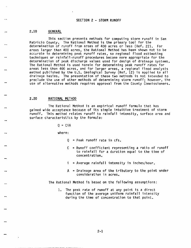
SECTION 2 - STORM RUNOFF
2.10 GENERAL
This section presents methods for computing storm runoff in San Patricio County. The Rational Method is the primary tool for the determination of runoff from areas of 400 acres or less (Ref. 22). For areas larger than 400 acres, the Rational Method has been shown not to be accurate in determining peak runoff rates, so regional flood estimating techniques or rainfall-runoff procedures become more appropriate for the determination of peak discharge values used for design of drainage systems. The Rational Method is used herein for determining peak runoff rates for areas less than 400 acres, and for larger areas, a regional flood analysis method published by the U.S. Geological Survey (Ref. 12) is applied to all drainage basins. The presentation of these two methods is not intended to preclude the use of other methods of determining storm runoff; however, the use of alternative methods requires approval from the County Commissioners.
2.20 RATIONAL METHOD
The Rational Method is an empirical runoff formula that has gained wide acceptance because of its simple intuitive treatment of storm runoff. This method relates runoff to rainfall intensity, surface area and surface characteristics by the formula:
Q = CiA
where:
Q = Peak runoff rate in cfs.
C = Runoff coefficient representing a ratio of runoff to rainfall for a duration equal to the time of concentration.
= Average rainfall intensity in inches/hour.
A = Drainage area of the tributary to the point under consideration in acres.
The Rational Method is based on the following assumptions:
1. The peak rate of runoff at any point is a direct function of the average uniform rainfall intensity during the time of concentration to that point.
2-1

2. The frequency of the peak discharge is the same as the frequency of the average rainfall intensity.
3. The time of concentration is the time required for the runoff to become established and flow from the most hydraulically remote part of the drainage area to the point under design. This assumption applies to the portion most remote in time, not necessarily in distance.
Although the basic principles of the Rational Method apply to drainage areas greater than 400 acres, practice generally limits its use to some maximum area. For larger areas, storage and subsurface drainage flow cause an attenuation of the runoff hydrograph so that the rates of flow tend to be overestimated by the Rational Method. In addition, the assumptions of uniform rainfall distribution and intensity become less appropriate as the drainage area increases. Because of the trend for overestimation of flows and the additional cost in drainage facilities associated with this overestimation, the application of a more sophisticated runoff computation technique is usually warranted on larger drainage areas. The designer should obtain permission from the County Commissioners before applying the Rational Method to areas larger than 400 acres. An example problem using the Rational Method is given following Section 2.23.3 (page 2-9).
2.21 Runoff Coefficient, C
The runoff coefficient, C, is the variable in the general equation of the Rational Method which is least susceptible to precise determination and thereby allows some independent judgement. However, uniform application of runoff coefficients can be achieved through the following considerations.
The runoff coefficient accounts for abstractions or losses between rainfall and runoff which may vary with time for a given drainage area. These losses are caused by interception by vegetation, infiltration into permeable soils, retention in surface depressions, and evaporation and transpiration. In determining this coefficient, differing climatological and seasonal conditions, antecedent moisture conditions and the intensity and frequency of the design storm should be considered.
2.21.1 Nature of Surface. The proportion of the total rainfall that will reach the outfall depends on the relative porosity or imperviousness of the surface, and the slope and ponding characteristics of the surface. Semi-impervious surfaces, such as asphalt pavements and roofs of buildings, will be subject to nearly 100 percent runoff, regardless of slope, after the surfaces have become thoroughly wet. On-site inspections and aerial photographs may prove valuable in estimating the nature of the surface within the drainage area.
2-2
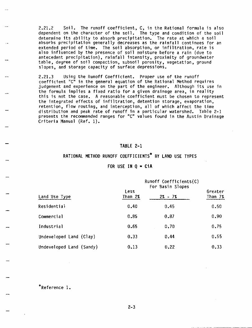
2.21.2 Soil. The runoff coefficient, C, in the Rational formula is also dependent on the character of the soil. The type and condition of the soil determine its ability to absorb precipitation. The rate at which a soil absorbs precipitation generally decreases as the rainfall continues for an extended period of time. The soil absorption, or infiltration, rate is also influenced by the presence of soil moisture before a rain (due to antecedent precipitation), rainfall intensity, proximity of groundwater table, degree of soil compaction, subsoil porosity, vegetation, ground slopes, and storage capacity of surface depressions.
2.21.3 Using the Runoff Coefficient. Proper use of the runoff coefficient "C" in the general equation of the Rational Method requires judgement and experience on the part of the engineer. Although its use in the formula implies a fixed ratio for a given drainage area, in reality this is not the case. A reasonable coefficient must be chosen to represent the integrated effects of infiltration, detention storage, evaporation, retention, flow routing, and interception, all of which affect the time distribution and peak rate of runoff in a particular watershed. Table 2-1 presents the recommended ranges for "C" values found in the Austin Drainage Cri teri a Manual (Ref. 1).
TABLE 2-1
RATIONAL METHOD RUNOFF COEFFICIENTS* BY LAND USE TYPES
FOR USE IN Q • CiA
Runoff Coefficients(C) For Basin Slopes
Less Greater Land Use T~~e Than 2% 2% - 7% Than 7%
Residential 0.40 0.45 0.50
Commerc i a 1 0.85 0.87 0.90
Industri a1 0.65 0.70 0.75
Undeveloped Land (C1 ay) 0.33 0.44 0.55
Undeveloped Land (Sandy) 0.13 0.22 0.33
* Reference 1.
2-3

It is often desirable to develop a composite runoff coefficient based in part on the percentage of different types of surfaces in the drainage area. The procedure is often applied to typical "sample" blocks as a guide to selection of reasonable values of the coefficient for an entire area. Suggested coefficients with respect to surface types are given in Table 2-2.
In contrast to the runoff coefficient values for storms of 10-, 25- and 100-year frequencies given in Table 2-2, the values in Table 2-1 are limited to 10- and 25-year frequencies. If Table 2-1 is used to determine the 100-year value, it should be adjusted upward accordingly.
2.22 Rainfall Intensity, i
Rainfall intensity, i, is the average rate of rainfall in inches per hour. Intensity is selected on the basis of design frequency of occurrence, a statistical parameter established by design criteria, and rainfall duration. For the Rational Method, the critical rainfall intensity is the rainfall having a duration equal to the time of concentration of the drainage basin.
Rainfall intensity in Corpus Christi, for example, can be determined for various return periods and durations from Figure 2-1, compiled by the U.S. Weather Bureau. These curves are applicable for design frequencies up to the 100-year storm and for durations from 5 minutes to 24 hours.
2.23 Time of Concentration
One of the basic assumptions underlying the Rational Method is that runoff is a function of the average rainfall rate during the time required for water to flow from the most hydraulically remote point of the drainage basin to the point under consideration. Time of concentration then is defined as the time it takes for runoff to travel from the hydraulically most distant part of the watershed to the point of reference. It is usually computed by determining the water travel time through the watershed. Overland flow, storm sewer or road gutter flow, and channel flow are the three phases of direct flow commonly used in computing travel time. Travel time can be estimated for various overland distances by entering Figure 2-2 with known watercourse slope in percent and reading velocity based on watershed ground cover characteristics.
2-4

TABLE 2-2
RATIONAL METHOD RUNOFF COEFFICIENTS· FOR COMPOSITE ANALYSIS
FOR USE IN Q • CfA
Runoff Coefficient (C) for Storm Frequency of
5 - 10 25 100 Character of Surface Years Years Years
Streets, Drives, and Parking Lots:
Paved 0.85 0.97 0.95 Unpaved 0.75 0.85 0.90
Roofs: 0.85 0.93 0.95
Lawns, Sandy Soil: Flat, 0-2% 0.07 0.08 0.09 Average, 2-7% 0.12 0.13 0.15 Steep, 7% or greater 0.30 0.33 0.37
Lawns, Clay Soil: Flat, 0-2% 0.18 0.20 0.22 Average 2-7% 0.22 0.24 0.27 Steep, 7% or greater 0.30 0.33 0.37
Undeveloped Woodlands and Pasture Land:
Sandy Soil:
Flat, 0-2% 0.12 0.13 0.15 Average, 2-7% 0.20 0.22 0.25 Steep, 7% or greater 0.30 0.33 0.37
Cl ay Soil:
Flat, 0-2% 0.30 0.33 0.37 Average, 2-7% 0.40 0.44 0.50 Steep, 7% or greater 0.50 0.55 0.62
* Reference 1.
2-5

~ ::l 0 J: ....... III W J: U Z .......
>-t: III Z w ... z
-1 -1
it z <{ 0:
20.0
15.0 -----10.0
8.0 I=-~ ---------::::::::::
6.0 =----= -------4.0
l- I=====-
2.0
-
1.0 -
0.8 f= ----0.6 ----
0.4 ----
0.2 -r-
0.1
FIGURE 2-1
RAINFALL INTENSITY-DURA nON-FREQUENCY
CURVES FOR CORPUS CHRISTI *
-
--I- --
---- - - - - - - - -- .
-e-- - - - - - -.-
~ ~I::s:--~ - - - .- - -
f====: I~t~~ t:---.-~ ~~~
~ ---- - -
~I"-I:::: ~ ~ , .......... "- ~IOO-YEAR
'''-", , .......... 1"- ~50-YEAR
Iv ~ Vj25-YEAR
-- --J.-
10 -YEA~::; V [)
~ ~ ---
5 -YEAR V ~~ 2-YEAR- ~~~~" ------ "" "'"' "--- "" f"<
" " '" I" " 1-. --- - - - - "" ",,--- '" f"<
" I" -~-~ ---- - - -" "--- " ,
'" -- -- - - - - - - - - '" -"
- 1- -
.-
5 6 10 15 20 30 405060 2 3 4 5 6 7 8 9 10 12
(HOURS) ( MINUTES) DURATION
* Referellce 5
2-6
18 24

()~
Z
I.J.l 0.. o
5U
I U
..J 5 rn ttl I, rn 0: 5 ) o !Y. ttl I-- 2 « 5:
.5
*
I I
II ,
I I ,
. I
f1eferenee 24
i
FIGURE 2-2
TnAVEL TIME VELOCITIES *
.5
I~ , I~
.. ~ - -
-- II
2
VELOCITY IN fUsee
2-7
I iii II
I! I',
) 4 5 I U

2.23.1 Overland Flow. The travel time for overland flow consists of the time it takes water to travel from the uppermost part of the watershed to a defined channel or inlet of the storm sewer system. Overland flow is significant in small watersheds because a high proportion of travel time is due to overland flow. The velocity of overland flow can vary greatly with the surface cover and tillage. If the slope and land use of the overland flow segment are known, the average flow velocity can be read from Figure 2-2. The travel time is then computed by dividing the total overland flow length by the average velocity.
Overland flow length should not exceed 300 feet for developed areas or 1,000 feet for undeveloped areas, before being intercepted by a defined channel or storm sewer inlet. Beyond these distances, use gutter flow or channel flow velocities from Figure 2-2 or a more rigorous analysis using Manning's formula.
2.23.2 Storm Sewer or Road Gutter Flow. Travel time through the storm sewer or road gutter system to the main open channel is the sum of travel times in each individual component of the system between the uppermost inlet and the outlet. In most cases average velocities can be used without a significant loss of accuracy. During major storm events, the sewer system may be fully taxed and additional channel flow may occur, generally at a significantly lower velocity than the flow in the storm sewers. By using the average conduit size and the average slope (excluding any vertical drops in the system), the average velocity can be estimated using Manning's formula (see Example 1).
Since the hydraulic radius of a pipe flowing half full is the same as when flowing full, the respective velocities are equal. Travel time may be based on the pipe flowing full or half full. The travel time through the storm sewers is computed by dividing the length of flow by the average velocity. If flow is principally in shallow road gutters, the curve for overland flow in paved areas shown in Figure 2-2 can be used to determine average velocity.
2.23.3 Channel Flow. The travel time for flow in an open channel can be determined by using Manning's equation to compute average velocities. Bankfull velocities should be used to compute these averages. Channels may be in either natural or improved condition.
2-8
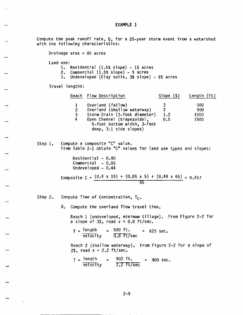
EXAMPLE 1
compute the peak runoff rate, Q, for a 25-year storm event from a watershed with the following characteristics:
Drainage area = 85 acres
Land use: 1. Residential (1.5% slope) - 15 acres 2. Commercial (1.5% slope) - 5 acres 3. Undeveloped (Clay soils, 3% slope) - 65 acres
Travel lengths:
Reach Flow DescriEtion SloEe {%) Len~th (Ft)
1 Overland (fallow) 3 500 2 Overland (shallow waterway) 2 900 3 Storm Drain (3-foot diameter) 1.2 1000 4 Open Channel (trapezoidal, 0.5 1500
5-foot bottom width, 3-foot deep, 3:1 side slopes)
Step 1. Compute a composite "C" value. From Table 2-1 obtain "c" values for land use types and slopes:
Residential - 0.40 Commercial - 0.85 Undeveloped - 0.44
Composite C = (0.4 xIS) + (0.85 x 5) + (0.44 x 65) = 0.457 85
Step 2. Compute Time of Concentration, Tc.
A. Compute the overland flow travel time.
Reach 1 (undeveloped, minimum tillage). From Figure 2-2 for a slope of 3%, read v = 0.8 ft/sec.
T = length = 500 ft. = 625 sec. velocity 0.8 ft/sec
Reach 2 (shallow waterway). From Figure 2-2 for a slope of 2%, read v = 2.2 ft/sec.
T = length = 900 ft. = 409 sec. velocity 2.2 ft/sec
2-9

B. Compute the storm drain flow travel time.
Reach 3. Use Manning's equation to compute pipe-full velocity.
V = 1.49 (R)2/3 (5)1/2 n
where:
R = A = (1.5~2 = 3 iTp 2 ( 1.) 4"
n = 0.015 for concrete conduit
5 = 0.012 slope
V = 1.49 3 2/3 (0.012) 1/2 = 9.0 ft/sec :orr 4"
T = length = 1,000 ft = 111 sec. velocity 9 ft/sec
C. Compute the open channel flow travel time.
Reach 4. Use Manning's equation to compute bank-full velocity.
V = 1.49 (R)2/3 (5f)1/2 n
where:
n = 0.040 for channel
R = A = 42 = 1.75 Wp 2""3-:-97
5f = 0.005 slope
V = 1.49 (1.75) 2/3 (0.005) 1/2 = 3.8 ft/sec 0.040
T = length = 1,500 ft = 395 sec velocity 3.8 ft/sec
D. Hence, the composite travel time, Tc = 625 + 409 + 111 + 395 = 1,540 sec = 26 min.
2-10

Step 3. Determine rainfall intensity. i.
For a duration equal to the time of concentration. 26 minutes, determine the 25-year rainfall intensity from Figure 2.1.
i = 4.6 in./hr
Step 4. Compute peak rate of runoff.
Q = CiA = 0.457 x 4.6 x 85 = 179 cfs
2.30 REGIONAL FLOOD ANALYSIS
Regional frequency analyses are used to develop procedures for determining peak runoff rates from areas that are hydrologically similar to locations within the region. In a regional frequency analysis, a region that is hydrologically homogeneous is defined, then hydrologic data from several locations within the region are grouped for hydrologic frequency analysis utilizing multiple regression techniques. Variables affecting the runoff characteristics of a region are tested for statistical significance, and only the ones that significantly affect runoff are retained in the regionalized equations.
Regression equations have been developed by the USGS for determining peak flood discharges for the 2-, 5-, 10-, 25-, 50- and 100-year frequency events for the coastal region of Texas (Ref. 12). These equations shall be used for drainage areas in excess of 400 acres unless other methods are approved by the County Commissioners.
The equations are in the form:
where:
Q = Peak discharge in cfs.
N = Return period in years.
B = Coefficient.
A = Uncontrolled drainage area in square miles.
x. y = Exponents.
S = Channel slope in ft/mi. This slope is the average slope of the streambed between the two points at 10 percent and 85 percent of the streambed length upstream of the point being analyzed.
2-11

For San Patricio County. the following equations will be used:
Q2 = 216 x (AO.574) x (SO.125)
Q5 = 322 x (AO.620) x (SO.184)
QlO = 389 x (AO.646) x (SO.214)
Q25 = 485 x (AO.668) x (SO.236)
Q50 = 555 x (AO.682) x (SO.250)
Q100 = 628 x (AO.694) x (SO.261)
Figures 2-3 and 2-4 are nomographs for determining the peak discharges.
2-12

FIGURE 2-3
NOMOGRAPH FOR 2, 5, AND 25 YEAR DISCHARGES *
0'" 3000 50,000
/
1000- 400
-100,000
10,000 -
- 50,000 100
VI 0 Z w 0 = 100 - 5000
~ lrl w VI
'" '" w « w -' a.. :J
tu ~ 0
'" VI ~ W
Z "--10,000 U >--iii w « ;:I w
w U u..
'" 1; z « 10 w w' W () - 5000
~ a.. « 0 z « -' 1000 ~
VI « '" a a
500
1000
- 1 - 500
100 0.3 0.3
100
* Reference 12
2-13

FIGURE 2-4
NOMOGRAPH FOR 10, 50, AND 100 YEAR DISCHARGES *
3000
.,Q /:eO /
500,000
200,000
1000 - 400 100,000
50,000
~ - 100,000 100
II) - 50.000 w . a
-' 100 Z i 0 w b:l IX II) W
« IX ~ :J 10,000 w ~ 0 "-
'" II) Ii:; w Z w "-
u. I-U w « a; w
w "-IX 5000 - ~ - 10,000 ::l
Z « u w z 10 w' ()
w' CL « 0 z () -' 10 5000 IX II) « «
IX J: 0 U
II)
a
1000
1000
500 1 -
500
0.3 0.3 ,.
100
100
* Reference 12
2-14

SECTION 3 - STREET FLOW
3.10 GENERAL
The location of inlets and permissible flow of water in streets is related to the frequency of traffic interference and the possibility of damaye to adj acent property.
Streets provide an important and necessary drainage service, even thouyh their primary function is for the movement of traffic. Traffic and drainage uses are compatible up to a point, beyond which drainage must be subservient to traffic needs.
Gutter flow in streets is necessary to transport runoff to storm inlets and to major drainage channels. Good planning of streets can substantially help in reducing the size of, and sometimes eliminating the need for, a stann sewer system in new developments.
3.2U EFFECTS OF STORMWATER ON STREET CAPACITY
The storm runoff which influences the traffic-carrying capacity of a street can be classified as follows:
Sheet flow across the pavement as falling rain flows to the edge of the pav~nent.
Runoff flowing adjacent to the curb or in roadside ditches.
Stormwater ponded at low points in streets.
Flow across the traffic lane from external sources, cross street flow (as distinguished from water falling on the pavement surface).
Splashing of any of the above types of flow on pedestrians.
Each of these types of storm water runoff must be contr'olled within acceptable limits so that the street's main function as a traffic carrier will not be unduly restricted.
The effects of each of the above categories of runoff on traffic movement are discussed in the following sections.
3.21 Interference Due to Sheet Flow Across Pavement
Rainfall that falls upon the paved surface of a street or road must flow overland as sheet flow until it reaches a channel. In streets with curbs and gutters, the curb and gutter become the channel, while on roads that have drainage ditches adjacent to them, the ditch becoilies the channel. The direction of flow on the street may be determined by the addition of the street grade and the crown slope. The depth of slleet flow
3-1

wi II be essentially zero at the crown of the street and wi II inCl'l'd';e as it proce!'ds towards the channel. Traffic interference due to sheet f low is essentially of two types, hydroplaniny and splash.
3.21.1 Hydroplaniny. Hydroplaniny is the phenomenon of vehich! tires actually being supported by a f11m of water that acts as a lubricdnl between the pavement and the vehi cl e. It generally occurs at spe('ds cOlllmon to freeways or arterial streets, or at turns. Its effect can he minililized either by installing relatively rough pavement that all0l1s water to escalle fronl beneath the tires (i.e., pavement grooving to provide drainage) or by reducing travel speed.
3.cl.c Splash. Traffic interference due to splash results frum sheet flow of excessive depth caused by water traveling a long d1stanc!' ur at a very low velocity before reachiny a gutter. Increasing the stn'et cro~m slope will decrease both the tin~ and d1stance required for water to reach the yutter. The crown slope, however, must be kept within acceptilhle limits to allow the openiny of doors when parked adjacent to curbs. An exceedingly wide pav~nent section contributing flow to one curb will also affect the depth of sheet flow. This may be due to superelevation of a curve, off-settiny of the street crown due to warping of curbs at intersections, or many traffic lanes between street crown and til!' gutter. Consideration should be given to all of these factors to maintain a depth of sheet flow within acceptable limits.
3.22 Interference Uue to Gutter Flow
Water that enters a street, either sheet flow from the pavement surfaCE! or overland flow from adjacent areas, will flow in the gutter of the street unti I it reaches some outlet, such as a storm sewer or a channel. As the flow progresses downhill and additional areas contribute to the runoff, the width of flow will increase and progressively infrinye upon the traffic lane. If vehicles are parked adjacent to the curb, the width of spread will have little influence on traffic-carrying cilpacity unti I it exceeds the width of the vehicle by several feet. However, on streets where parkiny is not permitted, as with many arterial streets, whenever the flow width exceeds a few feet it will significantly affect traffic. Field observations show that vehicles will crowd adjacent lanes to avoid curb flow.
As the width of gutter flow increases, it becomes irnpossible for vehicles to operate without driving through water, and they again Ileyin to use tire inundated lane. At this point the traffic velocity wi II be signi ficantly reduced as the vehicles begin to drive through the d{~eper water. Splash from vehicles traveliny in the inundated lane obsclJres the vision of drivers of vehicles moving at a higher rate of speed on the open lane.
Eventually, if width and depth of flow become great ellulI~h, the street will become ineffective as a traffic-carrier. Uuriny tllese Ileriods it is imperative that emeryency vehicles such as fire trucks, ambulances, and pol ice cars be able to traverse the street by moving along the crown of t he roadway.
3-2

lite street classification is also important when cOllsideriliU LIIE! degree of interference to traffic. A local street, and to a lesser extent a collector street, could be inundated with little effect upon vehicular travel. The small number of cars involved could move at a low r,ltl' of speed ttlrough the water even if the depth were four to six inches. However, reducing the speed of freeway or arterial traffic affects d great number of private, cOlllmercial, and emergency vehicles.
3.23 Interference Vue to Ponding
Storm runoft ponded on the street surface because of gl'alle change or ttle crown slope of intersecting streets has a substantial effect on the street-carrying capacity. A major problem with ponding is that it may reactl Ilepths greater then the curb and remain on the street for 101lU periods of time. Another problem is that ponding is localized in nature and vehicles may enter a pond moving at a high rate of speed.
The manner in which ponded water affects traffic is essentially the sallie as for curb flow; that is, the width of spread onto the traffic lane is the critical parameter. Ponded water will often bring traffic to a complete halt. In this case, incorrect design of only one facet of an entire street and storm drainage system will render the remainder of tIle street system ineffective during the runoff period.
3.24 Interference Vue to Water Flowing Across Traffic Lane
Whenever storm runoff, other than sheet flow, moves across a traffic lane, a serious impediment to traffic flow occurs. The cross-flow may be caused by superelevation of a curve or flow exceeding the calJacity of a higher gutter on a street with cross fall. The problem associated with this type of flow is the same as for ponding in that it is localized in nature and vehicles may be traveling at high speed when they n~ach the location. If the velocity of vehicles is naturally slow, and use is light, SUCII as on local streets, cross street flow does not cause sufficient interference to be objectionable.
The depth and velocity of cross street flow should always be maintained within such limits that it will not have sufficient force to affect moving traffic. If a vehicle that is hydroplaning enters all area or cross street flow, even minor force could be sufficient to move it laterally towards the yutter.
At certain intersections, the flow may be trapped betw[>(!n converging streets and must either flow over one street or be carried underground. If the vehicles coming to the intersection are already required to stop, then very little hazard exists to the traveling public. This is the basis for the assumption that cross pans are acceptahle across a local street where it intersects another local or collector street. Anotller point in favor of the use of cross pans is when the local street is allowed to coincide with the crown of the major street, the outsille traffic lanes of the major street have a built-in hump at the intersection.
3-3

3.2~ Effect on Pedestrians
In areas where pedestrians frequently use sidewalks, splilsh due to vellicles moving through water adjacent to the curb poses a serious, adverse sociological imJJact. It must also be kept in mind that under certain circumstances, pedestrians will be required to cross ponded or flowing water adjacent to curbs.
Since the majority of pedestrian traffic will cease dlJring the actual rainstorm, less consideration need be given to the problelll while the rain is actually falling. Ponded water, however, remaining after tile storm has passed, must be negotiated by pedestrians.
Streets should he classified with respect to pedestrian traffic as well as vehicular traffic. As an example, streets classified as local for vellicles but located adjacent to a school are arterials for peliestrian traffic. Allowable width of gutter flow and ponding should reflect this fact.
3.3U UESIGN CRITERIA
Uesign criteria for the collection and moving of runoff ~Iater on pub 1 ic streets is based on a reasonable frequency of traffic interference. That is, depending on tile character of the street, certain traffic larles can be fully inundated once during the initial design storm retlJrn period, usually orlce each ~~ years. However, during this JJeriod, lesser storms occur which will produce runoff and which will inundate traffic lanes to some sma 1 I er degree.
Planning and design for urban storm runoff must be corlsiliered from the viewpoint of both the regularly expected storm occurre'lce, that is, the initial storm, and the major storm occurrence. The initial storm will have a frequency of one in 2b years. Tile major storm will have a return period of IUU years. The objecti ve of the major storm runoff planning and design is to eliminate major damage and loss of life. The initiill drainage system is necessary to eliminate inconvenience, trequently recurring rninor damage, and high street maintenance.
3.31 Street Capacity For Initial Storms
Uetermination of initial storm-carrying capacity of the street is based upon two considerations: (a) pavement encroachment for computed theoretical flow conditions, and (b) an empirical reduction of tlH~ theoretical allowable rate of flow to account for practical field cond it ions.
3.31.1 Pavement Encroachment. The pavement encroachment for the initial storm shall be limited as set forth in Table 3-1.
The storm sewer system should commence at the point wherr! the maximum encroadhment is reached, and should be designed on the basis of the
3-4

*
**
TABLE 3-1
ALLOWABLE INITIAL STORM RUNOFF ENCROACHMENT
Street Classification
Loca 1
Collector
Arterial
Expressway
Init i al Storm Frequency
lU-year
lO-year
2S-year
2 - ** ~-year
Maximum Encroachillent
· * No curb over-toIJlllny. Flow Inay cover crown of street.
· * No curb over-topplny. Flow spread must leave at least one lane (12 feet) free of water fur a two-lane roadwny unll two lanes for a four-lane roadway.
· * No curb over-tollplny. Flow spread must leave at least one lane free of water in each direction.
No encroachment is allowed on any traffic lane.
Where no curbing exists, encroachment shall not extend over prollerty lines except at drainage easements.
~U-year for a depressed highway cross section.
3-!i

initial storm. Uevelopment of the major drainage system is enco\lr;l!J(~d so that the initial runoff is removed from the streets, thus movinlJ the point at Wllich the storm sewer system must begin to a point further llowrlstreanl.
3.31.~ Calculating Theoretical Capacity. When the allowable 1)~v(>lnent encroachillent has been determined, the theoretical gutter-carryin<j capacity for a particular encroachment shall be computed using the llIodifif'ci MafminlJ's formula for flow in shallow triangular channel, as shown in Figure 3-1.
Figure 3-1 nlay be utilized for all gutter configuratiofls. To simplify computations, graphs for particular street shapes may be plotted. An "n" value of U.UI6 shall be utilized for concrete curb and gulll'r unless special considerations exist.
3.31.3 Allowable Gutter Flow. The actual flow rate allowable per gutter shall be cal cuI ated by multiplying the theoretical capacity by the corresponding factor obtained from Figure 3-2. The deSigner will tllen be able to develop discharge curves for standard streets.
3.3~ Street Capacity For Major Storms
Uetermination of the allowable flow for the major storm is based upon two considerations: (a) theoretical capacity based upon allowable depth and inundated area, and (b) reduced allowable flow due to velocity considerations.
3.J~.1 Allowable Uepth and Inundated Area. The allowable depth and inundated area for the major storm shall be limited as set forth in Table 3-~.
3.J2.~ Calculating Theoretical Capacity. Based upon the allowallle depth and inundated area as determined from Table 3-2, the theoretical street-carrying capacity shall be calculated. Manning's formula shall be utilized with an "n" value applicable to the actual boundary conditions encountered.
3.3~.J /Illowable Flow for Major Storm. The actual flow al1o~lable within the street right-of-way shall be calculated by multiplying the theoretical caflacity by the corresponding reduction factor obtained from Figure 3-2.
3-6
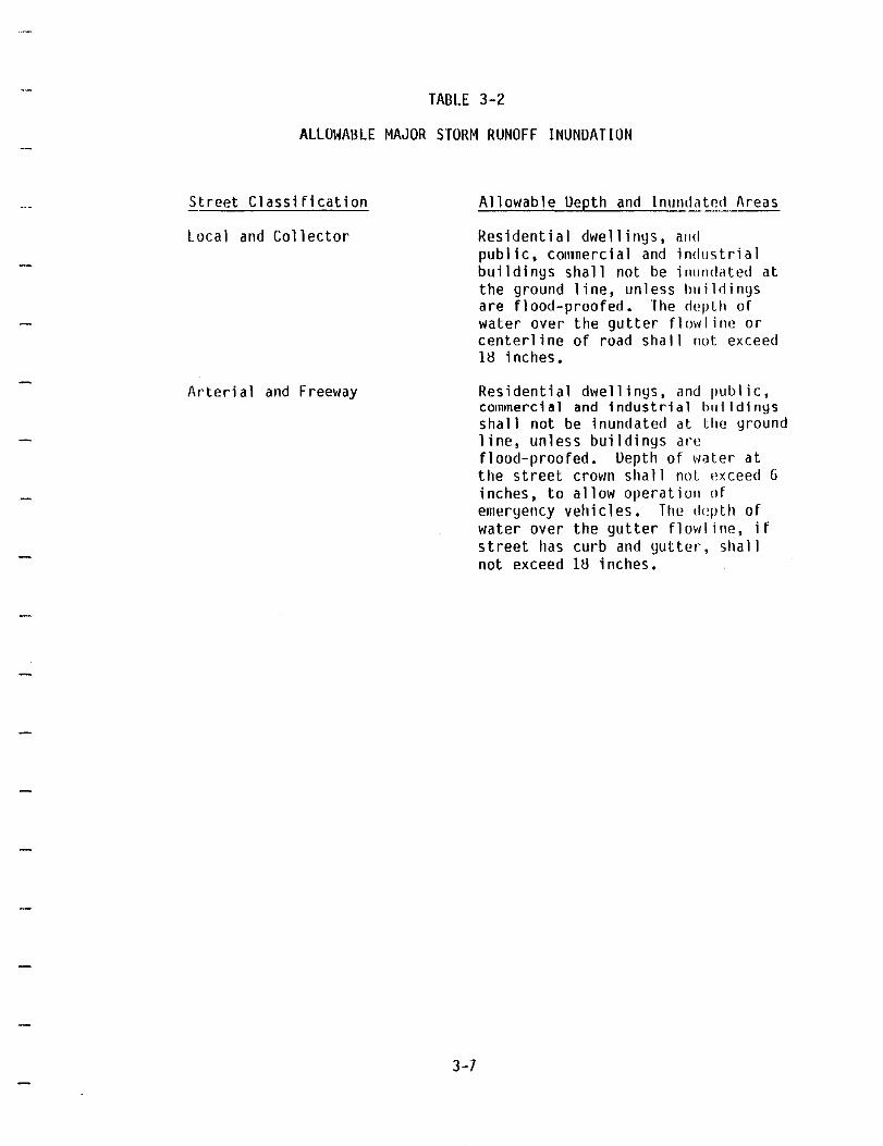
TABLE 3-2
ALLOWABLE MAJOR STORM RUNOFF INUNDATION
Street Classification
Local and Collector
Arterial and Freeway
3-7
Allowable Oepth and Inundated Areas
Resi dent i a I dwell i n\ls, and public, cOlllnercial and industrial buildin\ls shall not be inundated at the ground line, unless bllildings are flood-proofed. The delJlh of water over the gutter flowl irle or centerline of road shall nut exceed IH inches.
Residential dwellings, and public, commercial and industrial hlli Idlnys shall not be inundated at the ground line, unless buildinys are flood-proofed. Oepth of water at the street crown shall nol ~!xceed 6 inches, to allow operation of erneryency vehi cl es. The dl!pth of water over the gutter flowline, if street has curb and \lutter, shall not exceed IH inches.

o I<1 n:
10,000 ·9,000 ·8,000 ·7,000
6,000
5,000
·4,000
3,000
.- 2,000
-~OOO ,,00 BOO
- 700
600
500
'100
300
-200
100 90 80
·70
·60
50
·40
30
• 20
-10
FIGURE 3-1
NOMOGRAPH FOR FLOW IN TRIANGULAR CHANNELS
- 2.0
EOUATION: 0=0.56 (~I ,'/2 y8/3
z:nECIPROCAL OF TRANSVERSE SLOPE ~:COHfICIENT OF ROUOIINESS IN MANNING'S
.10 (iO%GRADE/
FonMULA ,:GnADE OF CIIANNEL IN FTIFT. ,=DEPHI AT CURe OR DEEPEST POINT IN FT.
w :z
EXAMPLE ISee do shed "~es)
GIVEN: 1=003
Z=24 ] Z/n:1200 n =.02 0:2.0 CFS
FIND: , :0.22
:J INSTRUCTIONS CJ ~ I. CONNEC T lfn nil 110 WII II SLorE II) 0: AND CONNEC r DISCIIARGE (0) WITH i= DErlll Iy). TIIESE TWO LINES MlJST
IN I EnsEC r AT WRNING LINE FOR COMPLE T E SOLU I ION.
100 :70 :50
- 30 -20
:10 II' : 7 b :5 :z ·3
P 2
lli : I 0: -,
~~5 u -If) .3 °.2
:.1 : .07 :.05
.03
.02
.01
-.08
- ,07
-.06
-.05
- .04
-.03
~-.02 ~ .
.. I· W Z Z <1 is -.01
"- -o
-.009 W
~ -.007 n: l!l
-.006
2. rOR 51IAU.OW V-SIIAPED CIIANNEL ~
-.005
AS SIIOWNLJSE NOMOGRIIPII 10 DE TERMINE DISCIIARGE IN SEC liONS o AND b SEPARATELY. THEN 0r'Oo+Qb
3. TO DE I ERMINE t -.eo--=". '_Y'~ DISCIIAIWE Q. IN -, -I-J b . ;;,,;,-" I'on lioN Of CIIANNEL Yl """" -'~I - (A) IIIIVING WID'" .: . -:'x~-:::- - -:- V DF:lEJ1MINE DEl'r" y FOn TOIIIL OISCIIIIJ1GE IN EN riflE SECTION n. T liEN USE NOMOGflAplI TO DETERMINE 0blN SECTION b Fon DEPnl
y" "'" .
IN COMpOSil E SECTION: ., u ,Ii,;,.,n,,;,-.m~ FOLLOW INS rRUCTIoN 3.
- .00'1
-.003
-,002
-1.0
- .BO
- .70
- .60
- .50
-.40
I· hI. hi -Il_
:z :- .30
Iz. o· n -.20 I-v, IJ' n. 'r! III (1
n: ()
01 n: -)
.' -.10 ~ 'f -.09 n. ~~ - .07
- .06
-.05
_ .04
-.03
-.02 4. TO DETERMINE DISCIIARGE b- . r Y' "
10 OBIAirl DISCI/IIRGE IN 1 ~_ J ,] .001 (O.I%GI1AOE/ SECTION 0 AI ASSlJMED x- 'tJ' DFrlll y; OIHAIN Qb fOn :ro(Y-Y'/ SLOPE RA 110 Zb AND DEPH' y'. 1I1EN Or: Qo • Qb·
.01 3-8

1.0
.9
.8
.7
a: o .6 f-u <1 LL
z o .5 1-u :J n lJ.) 4 a: .
.3
.2
.1
.0
FIGURE 3-2
REDUCTION FACTOR FOR ALLOWABLE GUTTER CAPACITY
- -. -- --- .-.- ,--'- ---
-
r r-s' 0.6°;' F, 0.8
1\ I-
\ - - -
9'0.4% ~ /" F' 0.5 V· - f- --I~
-
1\ , I
~ r .-1\
- -
1
I ~ 1- " I BELOW MINIMUM
~ t>- ALLOWABLE
_I STREET GRADE ~ - - --I ............. r--I --r--I I-
V a 2 4 6 8 10 12 14
SLOPE OF GUTTER (%)
3-9

3.33 Ponding
The term "ponding" refers to areas where runoff is reslr'ictCII to the street surface by sump inlets, street intersections, low points, intersections with drainage channels, or other reasons.
3.33.1 Initial Storm. Limitations for pavement encroachment by paneling for tile initial storm are those presented in Table 3-1. These I ililitations Shill I determine the allowable depth at inlets, gutter turnouts, culvert headw~ters, etc.
3.33.2 Major Storill. Limitations for depth and inundated area for nlajor storms are those presented in Table 3-2. These limitations shall determine the allowable depth at inlets, gutter turnouts, culvert headwaters, etc.
Where allowable ponding depth would cause cross street flow, the limitation shall be the minimum allowable of the two criteria.
3.34 Cross Street Flow
Cross street flow comes in two general categories: Tile first type is runoff that has been flowing in a gutter and then flows across the street to the opposite gutter or to an inlet; the second type is filM from some external source, such as a drainageway, which will flow across the crown of a street when the conduit capacity beneath the street is exceeded.
3.34.1 Uepth. Cross street flow depth shall be I imited as set forth in Table 3-3.
3.34.2 Theoretical Capacity. Based upon limitations in Table J-J and other ~IJplicable limitations (such as ponding depth), the theoretical quantity of the flow will vary, and no general rule for a computational method can be made. The Manning equation may be used with appropriate "n" value to estimate theoretical capacity; however, care should be taken in the determinat ion of flow boundaries.
J.3~.3 Allowable Quantity. Once the theoretical cross street capacity lIas been computed, the allowable quantity shall be calculated by multiplying the theoretical capacity by the corresponding factor from Figllre 3-2. The slope of the water surface crossing the street sllall be useei in lieu of the gutter slope.
3-1U
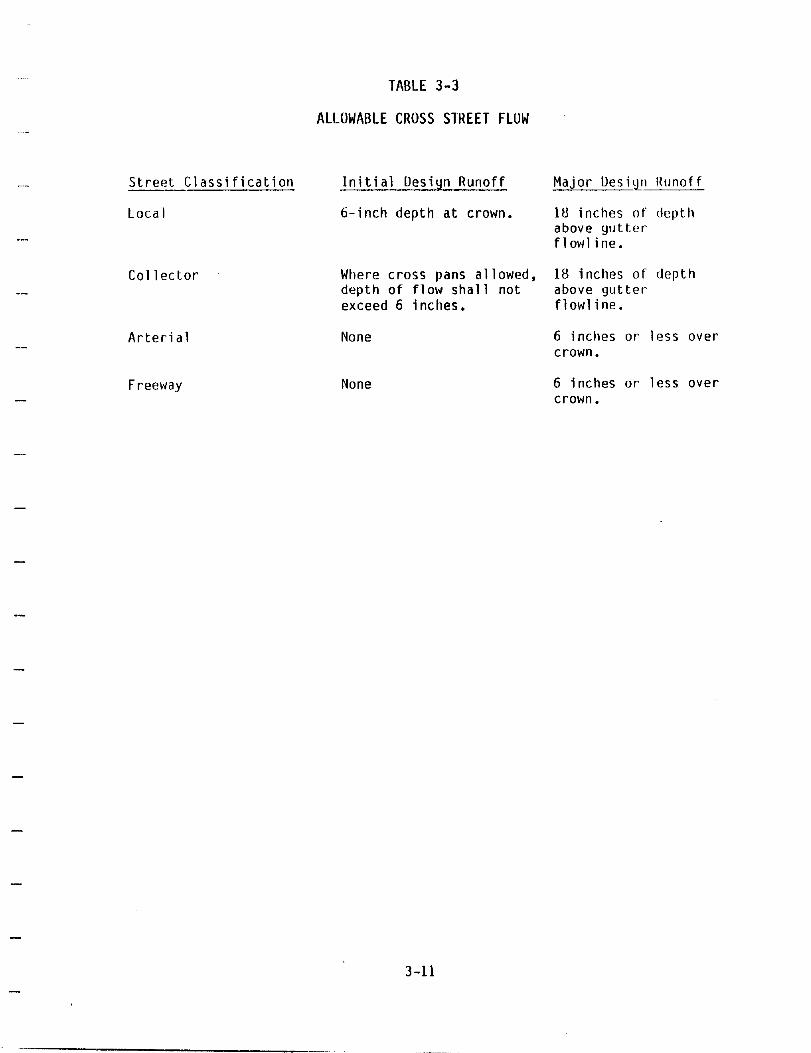
Street Classification
Local
Collector
Arterial
Freeway
TABLE 3-3
ALLOWABLE CROSS STREET FLOW
Initi al Desiyn Runoff
6-inch depth at crown.
Where cross pans allowed, depth of flow shall not exceed 6 inches.
None
None
3-11
Maj or Des i \l!l Runoff
H.! inches of depth above yutter flo.dine.
18 inches of depth above gutter' flowline.
6 inches or less over crown.
6 inches or less over crown.

3.4U INTERSECTION LAYOUT CRITERIA
The followiny desiyn criteria are appl icable at inters('cl ions of streets. Gutter carryiny capacity limitations covered previously sllall apply alony the street proper, while this section shall yovern at the intersection.
3.41 Gutter Capacity, Initial Storm
3.41.1 Pavement Encroachment. Limitations at intersections fur pavement encroachment shall be as yiven in Table 3-1.
3.41.~ Theoretical Capacity. The theoretical carryiny capacity of each gutter approachiny an intersection shall be calculated based upon the most critical cross section (see Figure 3-3).
A. Continuous Grade Across Intersection. When the Ylltler slope will be continued across an intersection, the slope used for calculatiny capacity shall be that of the gutter fluwline crossing the street.
B. Flow Direction Change at Intersection. When the Ylltter flow must undergo a di rection change greater than 40 d('yrees at the intersection, the slope used for calculating capilcity shall be the effective gutter slope, defined as th(' average of the gutter slopes at 0 ft., 2!:J ft., and OU ft. from the point of direction change.
C. FIOlI Intersection by Inlet. When yutter flo~1 will be intercepted by an inlet on continuous grade at the intersection, the effective gutter slope shall be IIti lized for calculations. Under this condition, the POillts for averaging shall be U ft., 25 ft., and 5U ft. upstredm frmn the i nl et.
3.41.3 Allowable Capacity. The allowable capacity for yutters approachiny an intersection shall be calculated by applying a reduction factor to the theoretical capacity.
A. Flow Approaching an Arterial Street. When the direction of flow is towards an arterial street, the allowable cdl"rying capacity shall be calculated by applying the reduction factor from Figure 3-2 to the theoretical gutter capacity. The grade used to determine the reduction factor shal I be the srune effective grade used to calculate the theoretical capacity.
3-12

PLAN
flGUIlE 3-3
INTERSECTION DRAINAGE - DESIGN CONSIDERATIONS
PLAN
L
USE GRIIOE OF cnoss 1'1111 ro'1 CAr.UlATlhO CAPACITY OF GUllEn AT I'DINTCD
FLOW UNE OF GUTTER
fONI'N
Gn40;~ I ;~~~·I-------~--------------I < ...... I- tlf4Ns I I-.......:.~
, CROSS PM~ Ol;40E ,--"----
-~~ TYPICAL SEC!'ON A-A f£tJ//,'-IJ~)I,!~ .
ItlTtRSEcTioN WIlEnE rLOW coNTINUOUS AcnosS IN cfloss PIIN E .....
TOP OF CUIlB
FLOW LlIIE _ TO cAI.CULATE CArMITY or Gill an H
OF GUIIER ~ 25' POINT (2), USE £FHcllVE SlOPE OOllllllEI) 50' BY AVEnAOINO SI.OPE .... T 0 r r, 25' /1110 5U'
f-------=-:"--. FROM INTERSECTION of 2 GUll EllS. OFT
TYPICAL SECTION 8 - B
INTERSECTION WlttRE FLOW MI.'ST MAKE DIf<ECTlON CHANGE
~ l----tINLET I ------ '/TOP OF CURB
:~""~~:,~~ ------E ,,' '3~'ONS IIErEsr,I\fIV TO OESIGII 1--0---=-'='--_ INU':T9 ON COII"NUOIJ~ Gn/lllr, Ilsr
50' ..... EFFECTIVE SLOPE OATAINEO flY /lVEIlI\O"'O OFT, SLorE AT 0 Fl,25'A!1050'fflOM CEllTEfl
OF INL E T.
TYPICAL SEC flON C-C
INTERSECTION WITII INLET ON CONTINUOUS GRAOE
3-13

B. Flow Approachin!) Streets Other Than Arterial. When the direction of flow is towards a non-arterial street, till' allowable carryin!) capacity shall be calculated by applying the reduction factor from Figure 3-2 to the theoretical gut ter capac ity. The slope used to determi ne the redllc t i on factor shall be the same effective slope used to calculate the theoretical capacity.
3.42 Gutter Capacity, Major Stann
3.42.1 Allowable Depth and Inundated Area. The allowable deptll and inundated area for the major stann shall be limited as set forth in Table 3-2.
3.42.2 Theoretical Capacity. The theoretical carrying capacity uf eacll gutter approaching an intersection shall be calculated, based upon the most critical cross section. The grade used for calculating capacity shall be based on guidelines presented in Section 3.41.
].42.] Allowable Capacity. The allowable capacity for gutters approaching an intersection shall be calculated by applying the reduction factor from Figure 3-2 to the theoretical capacity. The gutter gralle used to determine the reduction factor shall be the same effective grade used to calculate the theoretical capacity.
3.4] Ponding
].43.1 Initi al Storm. The allowable pavement encroachment for the initial storm shall be as presented in Table 3-1.
3.4].2 Major Storm. The allowable depth and inundated area for the major storm shall be as presented in Table 3-2.
3.44 Cross Street Flow
3.44.1 Oepth. Cross street flow depth at intersections shall I)e limited as set forth in Table 3-3.
3.44.2 Theoretical Capacity. The theoretical capacity shall be calculated at the critical point of the cross street flow. Where cross street flow will be conveyed across a local or collector street, tile cross-sectional area used for calculations shall be along the centerline of the local street. The slope shall be the slope of the cross pan at the point.
3-14
SECTION 4 - INLETS
4.10 GENERAL
The primary purpose of a storm drai n i nl et is to intercept excess surface runoff and deposit it in a drainage system, thereby reducirlY the possibility of surface flooding.
The most comlllon location for inlets is in streets that collect and channelize surface flow, making it convenient to intercept. I\pcause the prilnary purpose of streets is to carry vehicular traffic, inlets ~Iust be designed so as not to conflict with that purpose.
The following guidelines shall be used in the design of inlets located in streets:
1. MinimulII transition for depressed inlets shall be IU feet.
2. The use of inlets with a 5" depression is discoura~l!'d on collector, industrial and arterial streets unless the inlet is recessed.
3. When recessed inlets are used, they shall not interfere with the intended use of the sidewalk.
4. The capacity of a recessed inlet on grade shall be calculated as U.75 of the capacity of a similar Ullrecessed in I et •
5. Uesign and location of inlets shall take into cOllsiderdtion pedestrian and bicycle traffic.
6. Inlet design and location must be compatible with tile criteria established in Section 3 of this manual.
4.2U CLASSIFICATION
Inlets are classified into three major groups: inlets irl SIJlrlpS, inlets on grade witholJt gutter depression, and inlets on grade with gutter depression. Each of the three major classes includes several varieties, which are outlined here because of their wide use.
Inlets in Sumps
I. Curb Upening 2. Grate 3. Combination (Grate and Curb Opening) 4. Urop 5. Urop (Grate Covering)
4-1

Inlets on Grade without Gutter Depression
1. Curb Opening £. Grate 3. Combination (Grate and Curb Opening)
Inlets on Grade with Gutter Depression
1. Curb Opening £. Grate 3. Combination (Grate and Curb Opening)
Figure 4-1 shows typical inlet types, and Figures 4-2 lhrollgh 4-1; show specific inlet types (see pages 4-~ through 4-14).
4.30 INLETS IN SUMPS
Inlets in sumps are inlets in low points of surface (Irairldye to relieve ponding. Inlets with a 5" depression located in streets of less than one percent grade shall be considered inlets in sumps. The capaci ty of in lets in sumps must be known in order to determi ne the depth and wi dth of pontliny for a given discharge. The charts in this section Inay be used in tile design of any inlet in a sump, regardless of its depth of depression.
4.31 Curb Opening Inlets and Drop Inlets
Unsubmerged curb opening inlets and drop inlets in a s\l,np or low point are considered to function as rectangular weirs with a coefl icient of discllarge of 3.0. Their capacity shall be based on the following equation:
~ = 3.0(y)3/£ L
where:
~ = Capacity of curb opening inlet or capacity of drop inlet in cfs.
y = Head at the inlet in ft.
L = Length of opening for water to enter inlet in ft.
Figure 4-9 provides for direct solution of the above equation.
Curb opening inlets and drop inlets in sumps have a tefl(lI~ncy to collect debris at their entrances. For this reason, the calculatetl inlet capacity shall be reduced by 10 percent to allow for clogging.
4-2

fiGURE 4- I
INLET TYPES
4-3

4.32 Grate Inlets
A grate inlet in a sump coefficient of discharge of U.6U. following equation:
where:
can be considered an orifice with a The capacity shall be based 011 Lhl~
Q = Capacity in cfs.
Ag = Area of clear opening in sq. ft.
y = Uepth of flow at inlet or head at sump in ft,
The curve shown in Figure 4-1U provides for direct solution of tIle above equatioll.
Grate inlets in sumps have a tendency to clog when flows carry debris such as leaves and papers. For this reason, the calculated inlet capacity of a grate inlet shall be reduced by 25 percent to allow for clogging.
4.33 Combination Inlets
The capacity of a crnnbination inlet consisting of a grdll'~nd curb opening inlet in a sump shall be considered to be the sum of the capacities obtained frrnn Figures 4-Y and 4-1U. When the capacity of the gutter is not exceeded, the grate inlet accepts the major portioll of the flow. Under severe flooding conditions, however, the curb.inlet wil I accept most of the flow since its capacity varies with y1.5 whereas the capacity of a grate inlet varies as yU.5.
Combination inlets in sumps have a tendency to clog and collect debris at their entrances. For this reason, the calculated inlet capacity shall be reduced by 2U percent to allow for this clogging.
4.4U INLETS ON GRAUE WITHOUT GUTTER DEPRESSION
4.41 Curb Opening Inlets
The capacity of a curb inlet, like any weir, depends Ullon the head and length of overfall. In the case of any undepressed curll opening inlet, the head at the upstream end of the opening is the depth of flow in the gutter. In streets where grades are greater than 1 percent, the velocities are high and the depths of flow are usually small as there is little time to develop cross flow into the curb openings; therefor'~, unltellressed inlets are inefficient when used in streets of appreciable
4-4

slope, but may be used satisfactorily where the grade is low ilnd tit.· crown slope hiyh or the gutter channelized. Undepressed inlets do not inLerfl'l'f! with traffic and usually are not susceptible to cloyying. Inlets 1)11 yradr should be designed and spaced so that 5 to 15 percent of gutter 1101'1 reachiny each inlet will carryover to the next inlet downstream, provided the carryover is not objectionable to pedestrian or vehicular traIl ic.
The capacity of an undepressed inlet shall be determinl'd by use of Figures 4-11 and 4-12, obtained from the Texas Department of Hi:)hvlays and Public Transportation (Ref. 7). An example problem using tileS!' fiyures is included at the end of this section.
4.42 Grate Inlets On Grade
Undepressed grate inlets on grade have a greater hydraulic capacity than curb inlets of the same length so long as they remain unclogged. Undepressed grate inlets on grade are inefficient in comparision to grate inlets in sumps. Their capacity shall be till! capacity determined from Figure 4-11 reduced by 15 percent. Grate inlets should be so designed and spaced so that 5 to 15 percent of the gutter flow reaching each inlet will carryover to the next downstream inlet, provided the carryover is not objectionable to pedestrian or vehicular traffic.
Grates \~ith bars parallel to the curb should always be tlsed for the above described installations because transverse framing bars crrate splash which causes the water to jump or ride over the grate. Grdtes Ilsed shall be certified by the manufacturer as bicycle-safe. For f1O\~s on strerts with grades less than one percent, little or no splashiny OCCllrs reyardless of the direction of bars.
The calculated capacity for a grate inlet shall be red!lced by 25 percent to allow for clogging.
4.43 Combination Inlets On Grade
Undepressed combination (curb openiny and grate) inlets on grade have yreater hydraul ic capacity than curb or grate inlets of the same lenytll. In general, combination inlets are the most efficient of the three tYlles of undepressed inlets presented in this manual. Grates witll bars parallel to the curb should always be used. The difference betwren a combination inlet and a grate inlet is that the curb opening receives the carryover flow that falls between the curb and the grate.
Tile capacity of a combination inlet shall be considerell to be 9U percellt of the sum of the capacities as determined for a curb opening inlet and a grate inlet (allowing for reduction due to clogging).
4-5

4.5U INLETS ON GRAUE WITH GUTTER DEPRESSION
4.51 Curb Opening Inlets Un Grade
The depression of the gutter at a curb oIJening inlet Iwlow the normal level of the gutter increases the cross flow toward the opening, therehy increasiny the inlet caIJacity. Also, the downstream transition out of the depression causes backwater which further increases the amoullt of water captured. Depressed inlets should be used on continuous yrddes that exceell one percent, and their use in traffic lanes shall conform with requirelllents of Sectioll 3 of this mallual.
The depression depth, width, length and shape all have significant effects on the capacity of an inlet. Reference to Section 3 of this manual must be made for permissible gutter deIJressions.
The capacity of a depressed curb inlet will be determined by use of Fiyures 4-11 and 4-12.
4.~2 Grate Inlets Un Grade
The depression of the gutter at a grate inlet decreases the flow past the outs i de of a grate. The effect is the same as that when d curb inlet is deIJressed, namely the cross slope of the street directs tile outer portion of flow toward the grate.
The bar arrangements for depressed grate inlets on streets with grades greater than one percent greatly affect the efficiency of the inlet. Grates with longitudinal bars eliminate splash that causes tile water to jump clnd ride over the crossbar grates, and it is reconmended that grates have a Ininilnum of transverse or crossbars for strength and spacing only.
For low flows or for streets with grades less than one percent, little or no splashing occurs regardless of the direction of bars. However, as the flow or street grade increases, the grate with longitudinal bars becmnes progressively superior to the crossbar grate. A few slnall rounded crossbars, installed at the bottom of the longitudinal bars as stiffeners or a safety stop for bicycle wheels, do not materially affect the hydraulic capacity of longitudinal bar grates.
The capacity of a yrate inlet on grades less than one percent shall be the capacity detennined from Figure 4-11. The capacity of grate inlets on grades greater than one percent shall be YU percent of tile capacity determined from Figure 4-11.
Grate inlets in depressions have a tendency to clog whel] gutter flows carry debris such as leaves and papers. For this reason the calculated inlet capacity of a grate inlet shall be reduced by 2!J percent to allow for clogging.
4-6

4.03 Combination Inlets On Grade
lJepressed combination inlets (curb openiny plus yrate) h,lve yreater hydraulic capacity than curb opening inlets or grate Inlets of the same lenyth. Generally speaklny, combination inlets are the 1110St dficlent of the three types of depressed inlets presented In this manual. Grates with bars parallel to the curb should always be used for maximulII efficiency. The basic difference between a combination inlet and a yrate inlet Is that the curb opening receives the carryover flow that passes the curb and the grate.
The depression depth, width, length and shape all have a siynificant effect on the capacity of an inlet. Reference to Section 3 of this manual must be made for permissible gutter depreSSions.
The capacity of a crnnbination inlet shall be considered to be 9U percent of the sum of the capacity of a curb opening inlet and a yrate inlet (allowing for reduction due to clogging).
4-7

..Jc)
FIGURE 4-2
DEPRESSED CURB-OPENING INLET
--- flOW PAT TE fHl IN A SUMP
L2 : L, IN SUMP
r L, -'------------~-----------,
L-____ L_2 ____ ·I ______ ~ --
----~J)-
---- ---
dv-------- PLAN
---=======:::::::::::=======:11
'-'1--1 I r------, CI==~==------__
I I I :
,,-:...:.....:.-:. .
SECTION A-A
! --.
SECTION B-B
v 2 E :YO'2~- to
SECTION C-C
4-8

FIGURE 4-3
DEPRESSED GRATE INLET
...tAl --- FLOW PATTERN It! A SUMP ... ~ r Lz=L,INSUMP
___ t=----------~.~LIL-------------I----~L---.-I~.~----~Ll----~
..... ------------
PLAN
~I SECTION 8-8
• WaLi ~-
~ ~
~f~ • : ~ . , 1 "" " " .. f , ..
........ ~t~, ~!
"~"~ ~r I::
';" • ". • SECTION C-C
"0--
SECTION A -A
4-9

--
FIGURE 4-4
DEPRESSED COMBINATION INLET
L,
SECTION A-A
--- FLOW PATTERII HI A SUMP L! : L, IN SUMP
Lz j
~--I
III
PLAN
r: ,~-l SECTION 8-8
4-10
SECTION c-c
v 2 E'V .:JI_ to
29

Slope --~
Jr- Slope ..
FIGUHE 4-5
DROP INLET (Grate covering)
--1- - - - - -I--I I
I I I I I I I I
-I------~-
". -"
SECllON A-A
DROP INLET TYPE A-4
i iiJlJiiiillOliiillii UUUUUUUUUUU
It
Perimeter 01 Opening' 20 12b In Fill
Perlmeler 01 Opening' 2 0 12b In Feel
\;,; .... ; ;,~·:~·::·.;;';~67:2~~;I~~:ti .. ::~.:T:ri~~:;~7.~ •. ? I .. ~ '~l¥: . . . . . . . ~ .. '.:' .
.'
~m""",-=.,..",,.,.,..,,,,· . ~'. ~., ...•.. :-:'.~'. :.'~: .. '.'~.'::~. :\
SECTION A-A
4-11
y ·yola

FIGURE 4-6
UNDEPRESSED CURB-OPENING <RECESSED)
~-.... --- FLOW PAT I ElltJ IN A SUMP
l. til 1---------------' }-- - - ---- -\ '-------------,,(;1 • '-
./ "--:;::/'" I '- "-
1 --... -- // ~ .-----,----_----:-:-. ---------'1-1 -@r----------- /~ ~--------~-
PLAN
L~· ... :· ... ~=_ V :'.:.;~. ,;: .• : ;: •. : :'::~ :':"'-:r. WfL,· "' .. " . , .. LI ... .J t .... ~C::""" '.' . ·~fT'~ ... ,·4:: .. : J:: Of ::~~ .•.. ;: "'.:0.' ... , .:{
SECTION B-B
.. . -: .... • "I • _~.:.
SECllor~ C-C
4-12

•
FIGURE 4-7
UNDEPRESSED GRATE INLET
--- FLOW PATTERN IN A SUMP
-11_ . JJI~rf --
. I ~ -..,.----- ~ ------- -------------------- - ------
PLAN
SECTION
~ ~===~O~1:-7-7f~77 ;; J);; );--;;; , --=- ~ )'0
r-J7/7 r- -
SECTION c-c .
SECTION A-A y : Yo
4-13

FIGURE 4-8
UNDEPRESSED COMBINATION INLET <RECESSED)
--- FLOW PATTErlN IN A SUMP
~ ____ jlr---__ I 1----11
'[ 'l1li' 'rr~; =====~-~ ~ I . ,
' ____ -_-~ ___ ----- .---L~ _____ ~- _____ :_-~ ___ _
SECTION 8-8
SECTION C-C
SECTION A-A
y: Yo
4-14

FIGURE 4-9
CAPACITY OF UNSUBMERGED CURB OPENING INLETS AND DROP INLETS
1111111
1-2.0- , --1- 1-
hI W LL 1.5 I z
<.!l Z
I 1 . .0-- +. Z
W .0.9-,
a. O.B- I I 0 -I-
1- .0.7- 1-
I 1 ; ,. ~/ 3
I V Q/L'3.0r"2
II I V-,I Ii ,
I I
I , v.
I I ~ I
I I ,
l,l .0.6---l -I-- I Z
!;:t 0.5- I I
3: .0.4- -1-0 --l LL
LL 0.3 0
II I I---
I !
,
n. 0.2-W I -
0
,.:; 0 .15
11111111 Ii
,/ VV-
V-0.1
0 .1 015 .0.2 .0.3 .0.4 .0.5 0.6 0.7 0.8.0.91.0 1.5 2.0 3D 4.0 5.0 60 70 009.0 00 Q/L, RATIO OF DISCHARGE TO INLET OPENING LENGTH (cfs/FTl
4-15

FIGURE 4-10
CAPACITY OF GRATE INLETS
3.0 4.0 5.0 6.0 7.0 a.o 9.010 15 20 30 40 50 60 70 ao 90 100
Q/Ag I RATIO OF DISCHARGE TO AREA OF GRATE (cls/SQ FT)
4-16

FIGUflE 4- 1 1
CAPACITY FOR INLETS ON GRADE
4-17

FIGURE 4-12
CURVES TO DETERMINE RA TlO OF INTERCEPTED TO TOTAL FLOW FOR INLETS ON GRADE
I.O-TT:/ ~; i /-;-;-i IT'i"i'7i"'iT7TiTITTi"i'TiTITITiiTT:Ti"iT7iTiTT'il11 iTiTiii"TTTiTiiTiTiTiTiTiii~~~::::==wo-1
I i I I II I
o.g- I; i I
II! II 0.8- i ! I II .
§ I LL I .! <i 0.7- I ! i II f- '1' I o I"
f- II" / ~ .1 o 'I/I! f- 0.6- ,I.: I i o 11:1
~ Ililllil, o. !' /' !. Wt· ,.
II I
~ 0.5- ~ II i i ! II : I! i\11 I I o 0.4- ;:::: II 111I 1
' I·' /'1' o :: :;'1/1 Illj,.1 i= i "1 " « ! , I : I il,. 0:: ! I 'I II' I :. 0.3- , I: II i . ~ , .: :1/ '.' . a II I, " II I' I
0.2- i II ' j i I Iii I ' I' I i I I ' I III' , I i I
L=ACTUAL CURB OPENIIIO LEIIOTII (FT) LII =LENGTU OF CURB OPEIIiNG FOR 100%
INTERCEPTION (FT) Q=FLOW INTERCEPTED BY INLET OF
LENGTH L (chI Q II = TOTAL FLOW IN APPROACH OUTTER (cl.1
II=OUTTER DEPRESSION 1FT) ,=DEPTU OF FLOW IN APPROACU
OUTTER IFTI
OJ I: ,,IIi ! Iii I" III Ii 0- ~~~~~~~~~~~~-~i-----ri ----,'-----.,-----.,------
o 0.1 0.2 0.3 0.4 O.!! 0.6 0.7 08 0.9 1.0 LILa. RATIO OF CURB OPENING LENGTH TO CURB OPENING
LENGTH FOR 100% FLOW INTERCEPTION
4-18

4.60 Use of Figures 4-11 and 4-12
EXAMPLE 1
Given: Street Width = 30' Cross Slope = 0' Street Grade = 1.0X Qa in one yutter = 8 cfs
Determine: Capacity, Q, of a 10' curb inlet with 2.5" depression.
Step 1. From Figure 3-1 (Section 3) assuming z = 3 and n = 0.016, depth of flow in gutter is y = 4.6", or U.3~'.
Step 2.
Step 3.
Step 4.
Step 5.
Step 6.
Enter Fig. 4-11 with y = 0.38' and a = 2.5" and find corresponding Qa = 0.46.
La
Compute La = 8 = 17.4. lJ.45"
Compute L = 10 = 0.57. La 17.4
Enter Figure 4-12 with L = 0.57 and a = 0.55 arId find La y
corresponding ~ = 0.74. Qa
Determine Q frrnn q = 0.74. Qa
Q = U.74 x 8 = 5.9 cfs
4-19

EXAMPLE 2
Given: Street Width = 44' Cross Slope = U' Street Grade = 0.6% Qa in low gutter = 8 cfs
Determine: Length, L, of undepressed curb inlet required to intercept HUI of gutter flow (Q = 6.4 cfs).
Step 1. From Figure 3-1 (Section 3) assuming z = 44 and n = U.U16, depth of flow in gutter (y) = 4.32". or U.36'.
Step 2. Entering Figure 4-11 with y = 0.36 and a = 0, find corresponding ~ = U.155. La
Step 3. Determine La = 8 = 51.6.
Step 4.
Step 5.
U.155
Entering Figure L = U.4H.
4-12 with Q = D.H and a = 0, find corresponding
La' Qa y
Compute L from L = 0.48. L = 51.6 (0.4!.l) = 24.8'. Use L = 25. La
The following three steps will confirm this value of L. Use L = 25.
Step 6.
Step 7.
Compute L = 25 = 0.485. La 51.6
Entering Figure !L= U.81. (la
4-12 with L = 0.485 and a = 0, find corresponding La Y
Step 8. Compute Q from ~ = U.81. Q = 8(0.81) = 6.5 cfs. Qa
4-2U
SECTION 5 - STORM DRAINS
5.IU GENERAL
A general description of storm drainage systems and quantities of storm runoff is presented in Section 2 of this manual. It is the purpose of this section to consider the significance of the hydraulic elements of storm drains and their appurtenances to a storm drainage system.
Hydraulically, storm drainage systems are conduits (open or enclosed) in which unsteady and non-unifonn free-surface flow exists. Storm drains accordingly are designed for open-channel flow to satisfy as well as possible the requirements for unsteady and non-uniform flow. Steady flow cond it ions mayor may not be uniform.
5.20 VELOCITIES AND GRADES
5.21 Minimum Grades
Storm drains should operate with velocities of flow sufficient to prevent excessive deposition of solid material; otherwise, objectionable clogging may result. The controlling velocity is near the bottom of the conduit and considerably less than the mean velocity. Stann drains shall be designed to have a minimum mean velocity flowing full at 2.5 fps. Table 5-1 indicates the grades for both concrete pipe (n = U.UI2) and for corrugated metal pipe (n = U.U24) to produce a velocity of 2.5 fps, which is considered to be the lower limit of scouring velocity. The minimum slope for standard construction procedures shall be U.4U% when possible. Any variance must have prior approval.
5.22 Maximum Velocities
Maximum velocities in conduits are important mainly because of the poss i bil it i es of excess he eros i on on the storm drai n inverts. Table 5-2 shows the limits of maximum velocity.
5.23 Minimum Diameter
Pipes that are to become an integral part of the public storm sewer system shall have a minimum diameter of IH inches.
5-1

Pipe Size, 1 n •
IH
21
24
27
3U
36
42
4H
!)4
60
66
72
7H
H4
96
TABLE 5-1
MINIMUM SLOPE REQUIRED
TO PRODUCE SCOURING VELOCITY
Concrete Pipe Slo~el ftlft
U.UUlH
0.OU15
U.OO13
0.0011
U.UOU9
O.UUUl
U.UUU6
0.OUU5
0.UOU4
0.OU04
0.0004
0.OU03
0.00U3
0.U003
U.OUU2
5-2
Corrugated Metal Pipe Slo~e, ftlft
U.UUuU
0.UU4l)
0.OU41
O.UOJ~
U.UUJ1
0.UU24
U.OUZU
0.OU1u
U.UOI4
0.0012
o .UOll
0.OU1U
U.UUUl)
U.UUUl!
U.UUU7
TABLE 5-2
MAXIMUM VELOCITY IN STORM DRAINS*
Description Maximum Permissible Velocity
Culverts (all types) 15 fps
Storm Drains (inlet laterals) No Limit
Storm Drains (colI ectors) 15 fps
Storm Drains (mains) 12 fps
*Reference tl.
TABLE 5-3
ROUGHNESS COEFFICIENTS Un" FOR STORM DRAINS
Materials of Construction
Concrete Pipe
CorruYdted Metal Pipe
Plain or Coated
Paved Invert
Desiyn Coefficient
0.012
U,024
0,020
5-3
Ranye of Manniny Coefficient
0.011 - U.015
U.U22 - U.U2b
O.OW - U.022

5.30 MATERIALS
In selecting a roughness coefficient for concrete pipe, between 0.011 and 0.015, consideration will be given to the average conditions during the useful life of the structure. An "n" value of 0.017 for concrete pipe shall be used primarily in analyzing old conduits where alignment is poor and joints have become rough. If, for example, concrete pipe is designed for a location where it is considered suitable, and there is reason to believe that the roughness would increase through erosion or corrosion of the interior surface, slight displacement of joints, or entrance of foreign materials, a roughness coefficient will be selected which, in the judgement of the designer, will represent the average condition. Any selection of "n" values below the minimum or above the maximum for either monolithic concrete structures, concrete pipe or corrugated metal pipe, must have the written approval of the County Commissioners.
The coefficients of roughness listed in Table 5-3 are for use in the nomographs contained herein, or for direct solution of Manning's equation.
5.40 FULL OR PART FULL FLOW IN STORM DRAINS
5.41 General
All storm drains shall be designed by the application of the continuity equation and Manning's equation, which are shown respectively as:
Q = AV, and Q = 1.49 AR 2/ 3 Sf 1/2 n
where:
Q = Pipe flow in cfs.
A = Cross-sectional area of
V = Velocity of flow in fps.
n = Coefficient of roughness
pipe in ft2.
of pipe.
R = Hydraulic radius = A/Wp in ft.
Sf = Friction slope in pipe in ft./ft.
Wp = Wetted perimeter in ft.
/
Charts and nomographs can be used instead of the direct solutions for the above equations.
5-4

There are several general rules to be observed when designing storm sewer systems. When followed, they w111 tend to alleviate or eliminate the common mistakes made in storm sewer design. These rules are:
1. Select pipe size and slope so that the velocity of flow will increase progressively, or at least will not appreciably decrease, at inlets, bends, or other changes in geometry or configuration.
2. Uo not discharge the contents of a larger pipe into a smaller one, even though the capacity of the smaller pipe may be greater due to steeper slope.
3. At changes in pipe size, match the soffits of the two pipes at the same level rather than matching the flow lines.
4. Conduits are to be checked at the time of their design with reference to critical slope. If the slope of the line is greater than critical slope, the unit will likely be operating under entrance control instead of normal flow. Conduit slope should be kept below critical slope if at all possible. This also removes the possibility of hydraulic jump formation within the line.
5.42 Pipe Flow Charts
Figures 5-1 through 5-9 are nomographs published by the Texas Uepartment of Highways and Public Transportation (Ref. 7) for detennining flow properties in circular pipe, elliptical pipe, and pipe-arches. The nomographs are based upon an On" value of 0.012 for concrete and U.024 for corrugated metal.
For values of "n" other than 0.012, the value of Q should be modified to Qc by using the formula:
Qc = Qn (0.012) nc
where nc is the value of On" other than 0.012 and Qn is the flow from the nomograph based on n = U.UI2. This formula is applied as follows: If nc = U.015, use the value of Qn (based on n = 0.012) from the nomographs, and then multiply this by U.UI2/nc, or U.012/0.015 in this case.
5.50 HYDRAULIC GRADIENT AND PROFILE OF STORM DRAIN
In storm drain systems flowing full, all losses of energy through resistance of flow in pipes, by changes of mrnnentum or by interference with flow patterns at junctions, must be accounted for by the accumulated head losses along the system from its initial upstream inlet to its outlet. The purpose of accurate detenninations of head losses at junctions is to
5-5

include these values in a progressive calculation of the hydraulic gradient along the storm drain system. In this way, it is possible to determine the water surface elevation that will exist at each structure.
San Patricio County does not require the hydraulic grade line to be established for all storm drainage design. It is not necessary to compute the hydraulic grade line of a conduit run if: (1) the slope and the pipe sizes are chosen so that the slope 1s equal to or greater than friction slope and less than critical slope, (2) the inside top surfaces rather than the flow lines of successive pipe are lined up at changes in size, and (3) the surface of the water at the point of discharge will not rise above the top of the outlet. Subject to these constraints, the pipe will not operate under pressure and the slope of the water surface under capacity discharge will approximately parallel the slope of the invert of the pi pe.
Lacking these conditions or when it is desired to check the system against a larger flood than that used in Sizing the pipes, and if the tai1water is known, then the hydraulic grade line and energy shall be computed and plotted. The friction head loss shall be determined by direct application of Manning's equation or by appropriate nomographs in this section. Minor losses due to turbulence at structures shall be determined by the procedure of Paragraph 5.80. The hydraulic grade line shall in no case be closer to the surface of the ground or street than 2 feet unless otherwise approved by the County Commissioners. If the storm sewer system is to be extended at some future date, present and future operations of the system must be considered.
5.60 MANHOLE LOCATION
Manholes shall be located at intervals not to exceed 600 feet for pipe 30 inches in diameter or smaller. Manholes shall preferably be located at street intersections, conduit junctions, changes of grade and changes of alignment.
Manholes for pipe greater than 30 inches in diameter shall be located at points where design indicates entrance into the conduit is desirable; however, in no case shall the distance between openings or entrances be greater than 1,200 feet.
5.70 PIPE CONNECTIONS
Prefabricated wye and tee connections are available up to and including 24" x 24". Connections larger than 24 inches will be made by field connections. This recommendation is based primarily on the fact that field connections are more easily fitted to given alignment than are precast connections. Regardless of the amount of care exercised by the Contractor in laying the pipe, gains in footage invariably throw precast connections slightly out of alignment. This error increases in magnitude as the size of pipe increases.
5-6

5.8U MINUR HEAU LOSSES AT STRUCTURES
The following total energy head losses at structures Shilll be determined for inlets, manholes, wye branches or bends in the desiyn of closed conduits. See Figure 5-1U for details of each case. MinimulIl head loss used at any structure shall be O.lU foot, unless otherwise a~~roved.
Ttle basic equation for most cases, where there is both ll~stream and downstream velocity, takes the form as set forth below with the various conditions of the coefficient Kj shown in Tables 5-4, 5-~, and ~-b:
where:
hj = Junction or structure head loss in ft.
V1 = Velocity in upstream pipe in fps.
V2 = Velocity in downstream pi pe in fps.
Kj = Junction or structure coefficient of loss.
g = Acceleration of gravity, 32 ft/sec 2•
In the case where the upstream velocity is negligible, the equation for head loss becomes:
2 hj = Kj '!L
2g
Short radius bends may be used on 24" and larger pipes when flow must undergo a direction change at a junction or bend. Reductions in head loss at manholes may be realized in this way. A manhole shall always be located at the end of such short radius bends.
h-7

Case No.
I
II
III
IV
V
VI
VII
VI II
TABLE 5-4
JUNCTION OR STRUCTURE
COEFFICIENT OF LOSS
Description of Condition (See Figure 5-10)
Coefficient Kj
Inlet on Main Line*
Inlet on Main Line with Branch Lateral*
Manhole on Main Line with 450
Branch Lateral
Manhole on Main Line with 900
Branch Lateral
45 0 Wye Connection or cut-in
Inlet or Manhole at Beginning of Line
Conduit on Curves for 900** Curve radius = diameter Curve radius = 2 to 8 times diameter Curve radius = 8 to 20 times diameter
Bends where radius is equal to diameter 900 bend 600 bend 450 bend 22-1/20 bend
0.50
0.25
0.50
0.25
0.75
1.25
0.50 0.40 0.25
0.50 0.48 0.35 0.20
Manhole on line with 600 Lateral 0.35
Manhole on line with 22-1/20 Lateral 0.75
* Must be approved by Director of Engineering
** Where bends other than 900 are used, the 90 0 bend coefficient can be used with the following percentage factors applied:
60 0 Bend - 85%; 45 0 Bend - 70%; 22-1/20 Bend - 40%
5-8

The va I ues of the coeffi ci ent "K j" for determi ni ng the loss of head due to obstructions in pipes are shown in Table 5-5 and the coefficients are used in the following equation to calculate the head loss at the obstruction:
A * A.
1.05
1.1
1.2
1.4
1.6
1.H
2.U
2.2
2.5
2 'iL 2g
TABLE 5-5
HEAD LOSS COEFFICIENTS DUE TO OBSTRUCTIONS
A * K' J A.
0.10 3.0
0.21 4.0
U.5U 5.0
1.15 6.U
2.4U 7.U
4.UU /:l.U
5.55 !:I.O
7.U5 1U.OU
!:I.7U
K· J
15.0
27.3
42.U
57. U
72.~
HH.U
104.0
121.U
* A = Ratio of area of pipe to area of opening at obstruction. A.
5-9

The due to sudden Table 5-6 and calculate the
values of coefficient "Kj" for determining the loss of head enlargements and sudden contractions in pipes are shown in the coefficients are used 1n the following equation to head loss at the change in section:
hj = Kj ~,where V = velocity in smaller pipe. 29
Q..z.* U1
1.2
1.4
1.6
l.tl
2.0
2.5
3.U
4.U
5.U
1U.0
TABLE 5-6
HEAD LOSS COEFFICIENTS DUE TO SUDDEN
ENLARGEMENTS AND CONTRACTIONS
Sudden Enlargements. Sudden Kj
0.10
0.23
0.35
0.44
U.52
0.65
0.72
O.HU
0.84
0.H9
0.91
* ~ = Ratio of larger to smaller diameter Ul
5-10
Contractions, K· J
O.UH
O.lH
0.2 !>
0.:33
0.36
0.4U
0.42
U.44
0.45
0.46
0.47

5.90 UTILITIES
In the design of a storm drainage system, the engineer is frequently confronted with the problem of grade conflict between the proposed storm drain and existing utilities such as water, gas and sanitary sewer lines.
When conflicts arise between a proposed drainage syst~n and a ut i llty system, the owner of the ut l1lty system shall be contacted and made awa re of the confl i ct. Any adj ustments necessary to either the dra i nage system or the utility can then be determined.
5-11

FIGURE 5-1
UNIFORM FLOW FOR PIPE CULVERTS ~
1,000
i \ ~ \ ~
~ 5.0 - - 500 il <1.0- -400 a ...... ..,
:... 0.01 \ ~ 3.0- -300
1- \ ~ ~ e -:! -- -0.005 hI _
g; -0.00<1 ..J III
-0.003
0.002
-0.001
0.0005
\ g; 9 2.0 200
\ ~ ~ \ IN W
\ ~ ~ \ M M \ ~ -- ~ '\ 0.50':- -:... 50 a
\ . Q.40- -40
\ 0.3~
0.10
30
-- \ ..
10\
\ EXAMPLE
GIVEN: S: 0.02 FIND: ~/D' 0-20ch ~. D' 36" ICONCRETE)
SOLUTION
diD' 0.30 d' 0.30.3'. 0.9'
\ \ \
5-12
\ \
\
'\ '\ '\ FIILL
rWW
loJ I·· ~J It: U Z ()
~
12-
15-
N 0
i d l') ~ ~-
-12
-15
-IB
-21
'\ 070-"'- 060-:=
~.50-::
-4
/ /
lB- -24
0.'10 a ".- _ 30 ~ 0 30-· 24-
i· ''''-, 27~ =:: 0.20 "-,30-
0:\ - 42 :.~ 33-
21- - 27
w ::; 36- -48 <t I
0.10 ~ / -54 042 -
I FULL; -60
0.90 _ -!LOW 48-0.70 - 66
0.60-: / 54 - - 72
0.50- / 60- - 78
00
.40
-./ 66_- B4
i= -90 ~ 0.30 72 - _ 96
o 78 - -102 ~ / B'I- -lOA
0.20 - "" I 90- -120
/ 96-
102 -/ 10B-
/
114-0.10 120
/ /

FIGURE 5-2
CRITICAL DEPTH OF FLOW FOR CIRCULAR CONDUITS
II Ii
120
108
-102
-96
-90
-84
-78
-72
-48
~ -42 a: III , .. w ::I :! -36 o II
o 0-33
30
27
-24
-21
-18
-15
12
-3,000
2,000
-1,000
III 11:' c( :J: U en 15
-500
-400
00 --- 110
-40 II -
o -30
20
10
-5 -4
3
2
5-13
-0.99
:- 0.90
:-0.80
0.70
-------- ,----,'!? :- 0.50 " -
-0.40
-0.30
0.20

-120
-114
-108
-102
-96
-90
84
-78
-7~ - 66 "'1:1
~\ -60
-54
_ -48 .. .. Ii .E _ 42 It: w I-w :E - 36 <t a " - 33 a
-30
- 27
-24
-21
-18
-15
12
FIGUnE 5-3
VELOCITY IN PIPE CONDUITS
'" 40.0
3.0-
2.0-
1.0
5-14
0.10-
0.20-
o ~ rr
" :J? 0.30~
0.40 -..:
0.50-:
0.60-:
090~ 1.00

FlGUHE 5-4
UNIFORM FLOW FOR CONCRETE ELLIPTICAL PIPE
0..0.0.0.(1
0..0.0.1 JL 2
3 w N
4 d/RISE iii 38.60.
11- 0..2- "' -ILZ -4 ILIL JUl
fi «t " -0..0.0.2 ~w
10.- M ~Ul - 34.53 IL-
<II -e>:
'" _I-I .J
'" w -32. H
'" - " -0..0.0.3
20.- :! 87a136- - 29.45
30. -B2.128-
40. --1.00
-0..004 -iii 0.9 (Full Flow) - 27.42 110 \A. 7T .121-
!:! w 0.2 Z
-0..005 :J 72.113- - 2'1 .38
" iii Z I-' 100. Z 0.3- ~ "- - I\:: " 68.106-, III I-' j: - '!! r--"-
<II - 22.34 - e>: I
"' 0..4- '0 63.98-
IL '0 tD
o - " .J <II Ul ~
300 58.91- -19 x 30
-0.0.1 400 - -1.00 liDO.
0.9 (Full Flow) 53 x 83 -
48 x 76-10.0.0.
-0..02 43 x 68- -14 123 2000.
38 I 60.
-0.03
-0.0.4
-0.05
0..06 5-15

FIGURE 5-5
CRITICAL DEPTH FOR ELLIPTICAL PIPE
2,000 0.99 8T 0136-
820128 -
1,000-17 0121-
72 .113 -
- 0.95 68.106 -
eoo- 63.98 -
400 - 58 • 91 -
0.90. 300 - 53.83 -
- 0.85 200- 48.76 - Z <I "-VI
43. 68-.. w VI
-0.80 in
a: 100- I .. 38.60- u,
~ N W - III VI ~ - o.T5 l!)
Q: - a: III
"- <I "-:x: - :t: 34.53 - ii .- IJ
~ -O.TO 50- VI ..J
a 32 .49 -.{
a u
..J 40 - f-n. «
U 29 145 - J t_ 30 -
_I
0.65 w a: u 2T 0 42 -
20-24.38 --060
22 I 34-
- 055 10-
19.30 -
-050 15-
4 -
3 14 I 23 - 0.45
2
0.40
5-16

FIGURE 5-6
VELOCITY IN ELLIPTICAL PIPE
SIZE 14 x 23 !!fAlSE
1.00 Y
0.15
0.80
-19x30 1.0
3
22.34
15 2.0
- 24.38
- 27.42 10 3
iii II-
- 29.4!1 4 !!. >-
Z !I I-
Cf. -32x49 U
20 9 Ul
" W > w - 34 • !l3 Q40-Ul 30
0:: W
uJ 40 Z
N ::J 10 - w (J') - ~ uJ - 38.60 50 Il> 0:: Z IL - "-
z u a 0::
-' ::l <t I-u - 43.68 t= 20 IL
-' 0.30 -' w - 48.76
30
- 53.83 200 40
- !l8. 91 300 150
- 63.98 400
!l00 - 68.106
- 72 .113 0.20
- 77 x 121 1,000
- 82 .128
87.136 2,000
O.I~
5-17
O.OOO!!
- 0.001
- 0.002
- 0.003
- 0.004
- 0.005
E "-,- -!!;
IrS CI1
- 0.01
-0.02
- 0.03
-0.04
- O.O!!
-0.06
0.01
FIGur~E 5-7
UNIFORM FLOW FOR PIPE ARCH
2
3 -
4 -
5-
10-
20-
30 --iii
40 - lJ.. ~
!!O-hI
-I.? a:
-<{ _l:
100-
200-
300
400 -
500-
',000-=
2,000
U (tJ
6
III z :.i \!) Z Z It
~
5-18
0.1-
0.2-III (tJ
- a: "-
0.3- "
0.4-
O!!OS"':' 07-08 -1.00 0.9 (FULL FLOW)
LJI "-0..
PIPE-ARCH SIZE - 62.102
-!!4 • 88
- 45 M73
- 40.65
- 36.58 44 .72-
40 • 65 - - 31 • 51
36 • 58 - _ 27 • 43
LJI "-
31.50- "-
21.43 -
'8.29 -
13 • 22-
" • 18
11.1 -22.361-
III II:
-'3.22
-''"18
U Z o u

FIGURE 5-8
CRITICAL DEPTH OF FLOW FOR PIPE -ARCH 0.99
1,000 0.95-
62 '102 -!l00
-400 0.90-
-54.89 -300
-200 -45.13 0.80-
- 40-65 -100
- 36' 59 0.70- IIJ VI .. - a: ... ......
z - 31·51
~ -50 ;t: ct - ~-II. W n. UI III - 40. w .. a: _ 0
II) <I 0..60- ..J VI x- 30 u <\ a: - 21. 43 VI - U
0 I-Lo) -20 a: N Vi
- U
I - 22.36 u a: .. , -10 0.50-tol a IL
- 18.29
-!I
4
3 0..40-
-18' 22 2
11.18
0.30
5-19

Q. 1,000
.§g~-
62 '102
400
-300 - 151'66
-200
- 45.73
-100
- 40.65
-;;; -- 36' 56 .1! -50
\lJ l? --' 40 0:
Z <l -- 31' 51 J:
- 30 <I U n. III III 0 -.. w III -20 0:
-27'43 uJ N u; J: -10 u 0: <I - 22' 36 I
uJ n. 0:
-5
-4
- 16'29 -3
2
-13'22
FIGURE 5-9
VELOCITY IN PIPE -ARCH
Y-ISO
- 10
-30
-20
\lJ z -10 :J Iii C1 -
l? !!:: z Z ~ 0: ::> [j I- 0 -
-I \lJ
-IS >
-4
- 3
-2
5-20
!!L!!!~~ 0.15-
0.20-
0.30-
0.40-
-0.50-
0.60-
0.70-
0.60-
0.90-
1.00
\lJ VI 0: ..... ."
F I(JUIlE 5- I 0
MINOR HEAD LOSSES DUE TO
TURBULENCE AT STRUCTURES
p- .-- -- ~lIlIII1II
SECTION
CASE I
- - - --._-----
INLET ON MAIN LINE
NOTE for Any Typ. 01 Inl.l.
CASE Il
INLET ON MAIN LINE _. ______ •• _.~. __ • _ •••• _____ 4
WITII BHANC" LA' EnAL ~r---
!11 d I I ~ III
I , , , t i, ~
PLAN NOTE 2 2 ----. v2 0.35 v,
60° lalaral hi: -- - ---29 29
PLI\N --
_0,. vL f;-= . .;:;-=. ==
2EClIOrt
CASE III
MANHOLE ON MAIN LINE WITII 45° BRANCH LATERAL
----, 0 v,l 0.75v,2
22:t. laleral hJ : 2~ - 29-
SEC11()N --- ... - - -
CASE JlJ:
MANHOLE ON MAIN LINE ---_._----WITH 90° BRANCH LATEUAL
5-21

FIGURE 5-10 (Continued)
MINOR HEAD LOSSES DUE TO
TURBULENCE AT STRUCTURES
PLAN -- Z I Vz 0.75 v,
h q ch. (01 l Conn) = -- - --
~~j -W~~:'t 1·:':1- " 0, .
SECTION
CASE }[
45 0 WYE CONNECTION
OR CUT IN
J:! CASE JlII
CONOUIT ON 90 0 CURVES'
NOTE. lIeod loss applied 01 PC. lor lenglh of curve. ,
Radius' Dlo. 01 Pipe hi' 0.50 ~L 2g
v z Rodlu. , 12·11) 010 01 Pip. hi' 0.25 fq
Y z Rodiu.,11l-2010Ia 01 Pipe hl'0.40 2~
Rodlu.' G,eoler Ihan 20010.0' Pipe hJ'O
'Whpn curves other than 90 0 0re used. apply tt" following Inclo" 10 90ocurvt' •. 600 cu,.0 05 'Yo 45°cu' .... e 70% 22 )I,ocu ••• 40 %
5-22
-- : -- -- - --- - °1'V I .~~~~. 1D-.. --- -- 1- -. ----- - ..... y
PLAN
SECTION --~---
CASE 3[[
INLET OR MANHOLE AT
BEGINNING or LINE
CASE :VI[[
O"V, --
BENDS WHERE RADIUS IS
EQUAL TO DIAMETER OF PIPE
NOTE: Iteadlo .. applied 01 beglnlng 0' bInd • z
90° Bond hi '0.5° 2'0 y •
60 0 Band h,'O.43 ¥9 y,Z
450 Blnd h,'O.35 29 y z
221'.0 Bend hl'0.20 2~'
SECTION 6 - UPEN CIIANNEL FLOW
6.1U GENERAL
Upen channels for use in the major drainage system hdVI'
significant advantage in regard to cost, capacity, multiple lise tor recreational and aesthetic purposes, and potential for detention sLoraye. Disadvantages include right-of-way needs and maintenance costs. Careful planning and design are needed to minimize the disadvantages anll to increase the benefits.
The ideal channel is a natura"l one carved by nature OVPI' d long period of time. The benefits of such a channel are that:
Velocities are usually low, resulting in a longer tim(~ 01 concentration and lower downstream peak flows.
Channel storage tends to decrease peak flows.
Ma i ntenance needs are usua lly low because the channe I i ~ somewhat stabi 1 i zed.
The channel provides a desirable green belt and recrf'C1Lional area adding significant social benefits.
Generally speaking, the natural channel or the man-madf' cllilnnel that most nearly conforms to the character of a natural channel i <; the most efficient and the most desirable.
In many areas facing urbanization, the runoff has been so minimal that natural channels do not exist. However, small trickle patlls nearly always f'xist and these provide an excellent basis for location iliid construction of channels. Good land planning should reflect even these minimal trickle channels to reduce development costs and minirnizp drainage problplliS. In some cases the prudent utilization of natural water routes in the dl'velopment of a major drainage system will reduce the requirements for an undf'rground storm sewer system.
Channel stahility has become a recognized problem in 111'11,111
hydrology because of the significant increase in low flows and 1)I'ak storm runoff rates. A natural channel must be studied to determine t1IP lIIeasures needed to avoid future bottom scour and bank cutting. Erosion control measures can be taken at reasonable cost which will preserve thl! natural alJpeal'ance without sacrificing hydraulic efficiency.
6.2U CHANNEL UISCHARGE
6.21 Manning's Equation
Careful attention must be given to the design of drrlinJy(~
channel s to assure adequate capacity and minimum maintenance to overcolile
6-1

the results of erosion and silting. The hydraulic characteristics of channels can be determined by Manning's equation:
I} 1.49 A R2/3 Sf1/2 n
where:
Q Total discharge in cfs.
n = Coefficient of roughness.
A Cross-sectional area of channel in sq. ft.
R = Hydraul ic radius of channel in ft = /\. -W
p
Wp Wetted perimeter in ft.
Sf = Slope of the frictional gradient in ft/ft.
6.2~ Uniform Flow
For a given channel condition of roughness, dischar~JP dlld slope, there is only one possible depth for maintaining a uniform flow. fhi'> depth is the normal depth. When roughness. depth and slope are kllO\'m at a channel section, there can be only one discharge for maintaininu ,I uniform flow through the section. This discharge is the normal discharyr>.
in exact channel.
If the channel is uniform and resistance and gravity f(JI'(:es are ba 1 ance, the water surface wi 11 be para 11 e 1 to the bot tOll1 of the This is the condition of uniform flow.
Uniform flow is more often a theoretical abstraction than an actual ity. True uniform flow is difficult to find in the field or to obtain in the laboratory. Channels are sometimes designed on the assllmption that they will carry uniform flow at the normal depths, hut because of conditions difficult if not impossible to evaluate anli lIenee not takeo into account, the flow will actually have depths considerahly di fferent from uni form depth. The engineer must be aware of the filct that uni form flow computation provides only an approximation of what wi II occur.
6.23 Normal Depth
The normal depth is computed so frequently that it is convenient to use nomographs for variolJs types of cross sections to eliminilt:p the need for trial and error solutions, which are time consuming. Nomograllhs for uniform flow are given in Figures 6-1 and 6-2.
6-2

o p
.. " '" n
- () 115
- 0 114
- 003
- 002
-001
0009
"0000
-- 0007
- 0006
- 0005
:~ . ()()02 u,
u,
- 0 (JOI
- (1 (J(J(19
-- () oooa
- 00007
- 00006
-00005
- 00U01
- 0.0003
- 00002
FIGURE 6-1
UNIFORM FLOW FOR TRAPEZOIDAL CHANNELS
GIVEN
5' 0.003 0'1.000 n' U029 W'40 55'1:1
~1!~~PI E
flNU SOLUTION
d %, O.oB6
Ul
d'40 _,0.OB6 '314
100 =-90 -BO -70
-60
i!> -z z z .. ::E -10 ,.. =- 9
,~ -- e u _ 7
ILl -CJ - 6 no _
~ - 5 (J U1 o -4
" 0:_ 3
:;:-1 -09 -OB
-07
-- 06
0.5
NO T E: Prolocl horhonloliy Irom 1:1 Icolo 10 obloln ooluo. lor 2:1 Ihru 6:1
6-3
~
~
" ~ 1: I-0
~
::E a I-~-a m
" ~
--100
- 90
-BO
-70
-60
- 50
--- 30
-
-20
-10
-9
-a
-7
-6
-5
-4
3
SII>[ SlOPE 5 II0flilOIliAI 10 VEnllCAL
II ?I 3.1 4.1 5.1 6:1
-- - -002
-003
:- 004
-005
:-006
:-001
o~ - OOB
-- - 009
~ -010
Ul ()
f-.(
0-
,~ u
-020
- OBO

FIGURE 6-2
MANNING'S FORMULA NOMOGRAPH

6.30 DESIGN CONSIDERATIONS
Man-made channels should have trapezoidal sections of adequate cross-sectional areas to take care of uncertainties in runoff estimates, changes in channel coefficients, channel obstructions and silt accumulations.
Accurate determination of the "n" value is critical in the analysis of the hydraulic characteristics of a channel reach and should be based on experience and judgement with regard to the individual channel characteristics. Table 6-1 gives a method of determining the composite roughness coefficient based on actual channel conditions, and Table 6-2 provides additional guidance in the selection of "n" values for various types of channels and channel conditions.
Where practicable and depending upon the type of soil, unlined channels should have sufficient gradient to provide velocities that will be self-cleaning but will not be so great as to create erosion. Lined channels, drop structures, check dams, or concrete spillways may be required to control erosion that results from the high velocities of large volumes of water. Unless approved otherwise by the County Commissioners, channel velocities in man-made channels should not exceed 6 fps.
6.40 CHANNEL CROSS SECTIONS
The channel shape may be almost any type suitable to the location and to the environmental conditions. Often the shape can be chosen to suit open space and recreational needs that create additional sociological benefits.
6.41 Side Slope
Normally slopes shall be no steeper than 3:1, which is also the practical limit for mowing equipment. Rock or concrete lined channels or those which for other reasons do not require slope maintenance may have slopes as steep as 1-1/2:1.
6.42 Depth
Deep channels are difficult to maintain and can be hazardous. Constructed channels should therefore be as shallow as practical with due consideration of cost and available right-of-way.
6-5

TABLE 6-1
COMPOSITE ROUGHNESS COEFFICIENT "n" FOR CHANNELS*
nu - Materi al Invol ved
n1 - Degree of Irregularity
n2 - Variation of Channel Cross Section
n3 - Relative Effect Uf Obstructions
n4 - Vegetation
In - Degree of Meandering
* Ref e rence 10.
Channel Conditions
6-6
Earth Fine Gravel Coarse Grave I
Smooth Minor Moderate Severe
Gradual Alternating
Occasionally A lternat i ng
Frequently
Negligible Mi nor Appreciable Severe
Low Medium High Very Hi gh
Minor Appreciable Severe
Value
u.()~LJ
U.LJ(,4 O.U~U
O.UOl) U.LJU:' U.llIU U.LJ~U
U.UUlJ
U.UU:'
lJ.UIU - U.015
U.lJOU U.U\U - lJ.U15 U.U;'lJ - U.U:JU U .U4 U - U. U60
D.lJO:' - 0.U1U U.UIU - U.U2~ U.U;!5 - U.U5U U.(J:'U - U.1UU
1 • Ul)() 1 • I :,LJ 1. :JUU

TABLE 6-2
ROUGHNESS COEFFICIENT "n" FOR CHANNELS*
Type of Channel and Description
EXCAVATED OR DREDGED
a. Earth, straight and uniform 1. Clean, recently completed 2. Clean, after weathering J. Gravel, uniform section, clean 4. With short grass, few weeds
b. Earth, winding and sluggish 1. No vegetation 2. Grass, some weeds 3. Dense weeds or aquatic plants
in deep channels 4. Earth bottmn and rubble sides !l. Stony bottom and weedy banks 6. Cobble bottom and clean sides
c. Dray line-excavated or dredged
d.
e.
1. No vegetation 2. Light brush on banks
I~ock
1. 2.
cuts Smooth and uniform Jagged and irregular
Cilannels not maintained, weeds and brush uncut 1. Dense weeds, high as flow depth 2. Clean bottom, brush on sides ]. Same, highest stage of flow 4. Dense brush, high stage
* Reference 10.
6-7
Minimum
0.016 0.0113 0.022 0.022
0.023 0.U25
0.03U 0.0213 0.025 0.030
0.025 0.035
0.02S U.035
O.OSO 0.040 O. U45 0.0130
Nonna 1
0.0113 0.022 O. U25 0.027
U.025 0.030
O.OJS 0.030 U.UJS 0.04ll
o .ll2U ll.050
ll.ll35 0.ll40
O.UUO 0.U5ll O.OlU ll.100
r~a x i filum
lJ.020 O.lJ25 lJ.OJU 0.033
1l.O]O U.ll33
U.04U ll.lJJ!J 1l.IJlllJ U.OSO
U.UJ] U.UGU
().040 U.USU
lJ.12U U.UUU 1l.1l0 O.14U

TABLE 6-2 (cont. )
Type of Channel and Uescription
NATUHAL STREAMS
a. Minor streams on plain (top width at flood stage < IUU feet)
1. Clean, straight, full stage, no rifts or deep pools
2. Same as above, but more stones and weeds
J. Clean, winding, some pools and shoals
4. Same as above, but some weeds and stones
~. Same as above, lower stages, more ineffective slopes and sections
b. Same as 4, but more stones I. Sluggish reaches, weedy,
deep pools tl. Very weedy reaches, deep
pools, or floodways with heavy stand of timber and underbrush
b. Flood plains
1.
2.
J.
Pasture, no brush Short grass High grass
Cultivated areas No crop Mature raw crops Mature field crops
Brush Scattered brush, heavy weeds Light brush and trees, in winter Light brush and trees, in summer Medium to dense brush, in winter Medium to dense brush, in su~"er
Trees Uense willows, su~"er, straight Cleared land with tree stumps,
no sprouts Same as above, but wi th heavy
growth of sprouts
6-U
Minimum
U.U2b
U.UJU
U.UJJ
U.UJ~
U,U4U U,U4b
U,UbU
U,U7b
U.U2S U.U3U
U,U2U U.U2S U,UJU
O,UJS U.03S O,U4U U.U45 U.U7U
U,l1U
U.U3U
U,U~U
Normal
U.UJO
U.U3b
U,U4U
U.U4b
U.U4B U,USO
U.O/U
O,lUU
U.OJU U,03~
ll,UJU 0,035 U,04U
U,USU U.()SU U.lJbl) lJ,U/U U.IUU
U, 1 SU
U.U4U
U,UbU
f'iaxillllllll
U.UJJ
U.U4U
u ,U4~
U.U~U
lJ.lJ~~
U,UtiU
U.UUU
U. I SU
U.lJJS Il.U5U
U.UiJU U.U4b U,UbU
U.lJ/ll ll.lJ6lJ ll.llUl) 1l.110 lJ,16U
ll.2Ull
lJ.UbU
ll.UUU

TAllLE 6-2 (cant. )
Type of Channel and Uescription Minimum
Heavy stand of timber, a few down trees, little undergrowth, flood stage below branches U.U~U
Same as above, but with flood stage reaching branches U.IUU
LINEU UR BUILT-UP CHANNELS
a. l:cJrruyated metal
b. Concrete I. Trowel finish c. Float finish J. Fi ni shed, wi th gravel on bottom 4. Unfinished ~. Gunite, good section b. Gunite, wavy section / • On good excavated rock u. Un irregular excavated rock
c. Corlcrete bottom float finished with sides of 1. Uressed stone in mortar c. Random stone in mortar J. Cement rubble masonry, plastered 4. Cement rubble masonry ~. Ury rubble or riprap
d. Gravel bottom with sides of I. Formed concrete
e.
f.
2. Random stone in mortar J. Ury rubble or riprap
I\spha I t 1. Smooth ;'. Rough
Vegetated
6-9
u.un
U.Ul1 U.U13 U.UI~ U.UI4 U.UI6 U.UW U.UI7 U.U22
U.Ul~
U.U17 U.UI6 U.U2U U.U2U
U.UI7 U.U2U u.un
U.UI3 U.UI6
U.UJU
Norma 1
U.IUU
U.12U
U.U2~
U.U13 U.UI~ U.UI7 U.U1/ U.UIY U.U22 U.U2U U.U21
U.lJI! U.U2U U.U2U U.lJ2~ U.UJU
U.lJ2lJ U.lJ2J U.UJJ
lJ.U13 U.Ulb
Haximlll11
U.UU
IJ. I bU
IJ.UJU
IJ.UI~
lJ.IJl6 U.U2U U.U2lJ U.U"J lJ.U2~
lJ.02U lJ.U211 0.U24 U.UJU U.UJ~
U.LJ2~ LJ.LJ26 U.UJb
U.~LJU

b.4J Bottom Width
Channel s with narrow bottoms are di fficult to mai ntdi n (lIld are conducive to high velocities during high flows. It is desirable tt) design open channels such that the bottom width is at least twice the df'pth, with b tu U times the depth desirable if consistent with cost and design constraints.
b.44 Trickle Channels
The low flows, and sometimes base flows, from dp.velopetl clreas mllst be given speci fic attention. If erosion of the bottom of til!' channel appears to be a prublem, low flows shall be carried in a trickl(~ channel that has a capacity of 5.0 percent of the design peak flow. Care must be taken tu insure that low flows du not create an erosion problem.
b.4J Freeboard
For channels with flow at high velocities, surface roughness, wave action, air bulking, and splash and spray are quite erosive ~Iony the tup of tile flow. Freeboard height should be chosen to provide a suitable safety Illaryin. The height of freeboard shall be a minimum of orle foot, or pruvide an additional capacity of approximately one-third of the "f'si~n flo~1. From Hef. 1, the formula for deep flows with high velociti('s is:
Freeboard (in feet) = 1.U + U.U25 vul/ J
where:
v = Velocity of flow in fps.
u = Depth of flow in ft.
For tile freeboard of a channel on a sharp curve, extra hei ght must he added to the outside bank or wall in the amount:
H=V2(T+B) 2gH
where:
II = Additional height on outside edge of channel ill tt.
v = Velocity of flow in channel in fps.
T = Width of flow at water surface in.ft.
B = Bottom width of channel in ft.
H = Centerline radius of turn in ft.
g = Acceleration of gravity, J( ft/sec(.
If H is equal or greater than J x B, additional freeboard is not re(luirect.
b-lU

6.5U CHANNEL UROPS
The use of channel drops permits adjustment of channel 'JI'ddients that are too steep for the desiun conditions. In urban drainaUl' ~1{)l'k it is often desi rabl e to use several low head drops in I iell of a few hi '1hpr drops. Special attention must be given to protectinu the channel froll1 erosion in the area of channel drops.
The use of sloped drops will generally result in lower cost installations. Sloped drops can easily be designed to fit the chclllnel topoyraphy.
Sloped drops shall have roughened faces and shall be no steeper than ~: 1. They shall be adequately protected from scour and not Cduse an upstrealll water surface drop that will result in high velocities IIpstream. Side cutting just downstream from the drop is a cOlllmon problem th,lt l'IUSt be protected against.
The length L will depend upon the hydraulic characterisfics of the chilnnel and drop. For a flow of 3U cfs/foot of width, L wOlild be about 1!:J fed, that is, about l/~ of the flow value. L should not be 1['ss tlliln lU feet, even for low flow values. In addition, followup riprappilllj wi II oftE'n ile necessary at most drops to more fully protect the banks alld channel bottom.
For additional information on drop spillways, consult the Nation,'!L Engineering Handbook, Section 11, Urop Spillways, SCS R~~port No. SeS/ENG/NEII-ll NTIS Accession No. PB243645/AS.
6.6U SUPERCRITICAL FLOW
Supercritical fiovi in an open channel in a developed ar['.! creates certain hazards which the designer must take into consideration. From a practical standpoint it is generally not possible to have any C1Jrvature in suctl a cllannel. Careful attention must be taken to insure against excessive oscillatory waves which may extend down the entire lenuth of the channel frolil only minor obstructions upstream. Imperfections at Joints of lined channels may rapidly cause a deterioration of the joints, in which case a complete failure of the channel can readily occur. In addition, high velocity flow entering cracks or joints creates an uplift force by the conversion of velocity head to pressure head which can dal!lage the cllannel lininy. It is evident that when designiny a lined channel with supercritical flow, the desiyner must use utmost care and consider all relevarlt factors.
6-11

SECTION 7 - CULVERT DESIGN
7.10 GENERAL
The function of a drainage culvert is to pass the design storm flow under a roadway or railroad without causing excessive backwater and without creating excessive downstream velocities.
7.20 DESIGN CRITERIA
The design flow shall be determined by methods described in Section 2.
7.21 Design Frequency
Culverts shall be designed to pass the 25-year runoff with a 2-foot freeboard and no flow over the roadway for areas with a drainage area of less than 5 square miles. Culverts with a drainage area of over 5 square miles shall be designed to pass the lOO-year frequency flood event.
At the option of the County Commissioners, the designer may design culverts as storm sewers with a 10-year design frequency. Under this option, the proposed culvert shall be placed on line and grade to permit connection to the future storm sewer. The major storm impacts shall be investigated for both the culvert configuration and the proposed storm sewer configuration. The major storm analysis of the storm sewer shall include upstream and downstream reaches sufficient to show that provisions for the major storm can be made when the storm sewer is constructed.
In areas where an official floodway exists, increases in the lOO-year water surface elevation shall not be greater than 1 foot above the natural lOO-year water surface elevation.
7.22 Culvert Discharge Velocities
The velocity of discharge from culverts should be limited as shown in Table 7-1. Consideration must be given to the effect of high velocities, eddies or other turbulence on the natural channel, downstream property and roadway embankment.
It is recommended that a mlnlmum velocity of 2.5 feet per second be maintained in all drainage structures to prevent siltation. Where doubt exists concerning silt or scour, protection commensurate with the value of the structure and surrounding property shall be installed to insure that damage to or failure of the structure will not occur.
7-1

TABLE 7-1
CULVERT DISCHARGE VELOCITY LIMITATIONS
Maximum Downstream Condition
A 11 owab Ie Di schill~f' Velocity (fps)
Earth Sod Earth
6 fps U fps
1 S fps Paved or Riprap Apron
7.3U CULVERT TYPES
Culverts shall be selected based on hydraulic principles, ('conolllY of size and shape. and a resulting headwater depth that will not Cillise dallla~(~ to adjacent property. It is essential to the proper desiyn of a cllI vl'rt that the conditions under which the culvert wi 11 operate <lre kno~ln. Critic,ll depth of flow for circular and rectanyular culverts can Ill' detel'lnined using the nomographs in Figures 7-7 and 7-tl (see pa~('s '/-11 and 7-1£'), illid these depths, de. are to be applied to the sample prohlpllls that foil O~I.
Six distinct types of operating conditions as classified hy th!! Texas ill'partment of lIiyhways and Public Transportation (Ref. 7) an' i IlustraLed and discussed on the following pages.
7.31 Mild Slope Regime, Critical Depth Control (Outlet Control)
FIGURE 7-1
HW< 1,50
CONDIT IONS
lhe entrance is IInsubmerged (HW < l.SD), the critical depth is less than uniform deptll at (lesign discharge (de < dul, and the tailwater is less than or equal to critical depth (TW ~ de)'
7-2

The above condition is a common occurrence where the naLllrd I channels are on flat grades and have wide, flat floodplains. Til(' control is critical depth at the outlet.
[n culvert design, it is generally considered that till' IH'cldwater paul maintains a constant level during the design storm. If this level does not submerge the culvert inlet, the culvert flows part full.
If critical flow occurs at the outlet, the culvert is said to have "outlet control." II culvert flowing part full with outlet control wi 11 requi re a depth of flow in the barrel of the cu lvert greater than critical depth while paSSing tllrough critical depth at the outlet.
The capacity of a culvert flowing part full with outlet control and tili lwater depth below critical depth is governed by the follov/iny equation when the approach velocity is considered zero.
HW = dc + Vcc. + he + hf - SoL 2g
where:
HW Headwater depth above the invert of the IIpstream end of the culvert in feet. Headwater IIlIlSt be equa 1 to or 1 ess than 1. 5U or entrance is submerged and another type of operatiorl will resul t.
dc = Critical depth of flow in ft. (see Figure I-lor /-U) •
U = Uiameter of pipe or height of box in ft.
9 = Acceleration of gravity, Je. ft/secC..
Vc Critical velocity in fps occurring at critical depth (see Figures I-I and I-U).
he Entrance head loss in ft.
e. he = Ke ~ e.g
Ke = Entrance loss coefficient (see Table I-L).
hf = Friction head loss in ft = SfL.
Sf = Friction slope or slope that will produ(!' uniform flow. For this type of operation, the friction slope is based upon 1.1 dc •
So Slope of culvert in ft/ft.
l length of culvert in ft.
7-3

TABLE 7-2
CULVERT ENTRANCE LUSS CUEFFICIENTS
Type of Structure and Design of Entrance
Pipe, Concrete
Projecting from fill, socket end (groove-end) Projecting from fill, sq. cut end lIeadwall or headwall and wingwalls
Socket end of pipe (groove-end) Square-edge Rounded (radius = 1/120)
Mitered to conform to fill slope *End-Section conforming to fill slope
Ileveled edges, 33.7-degree to 4~-degree bevels Side- or slope-tapered inlet
Pipe or Pipe-Arch, Corrugated Metal
Col'fticient Ke
u. cO 0.50 U • clJ U.11J o . 50 tJ.2U 0.20
Projecti ng from fill (no headwall) U. YO IIpa(h~a II or headwa 11 and wi ngwa 11 s square-edge O. 5U r,litered to conform to fill slope, paved or unpaved slope 0.70
*[rld-Section confonning to fill slope o.~o Ileveled edges, Jj.7-degree to 45-degree bevels II.cU Side- or slope-tapered inlet 0.20
Box, Reinforced Concrete
lIeadwall parallel to embankment (no wingwalls) Square-edged on 3 edges U.~U Rounded on 3 edges to radius of 1/12 barrel
dimension, or beveled edges on 3 sides U.2U Wingwalls at 30 degrees to 7~ degrees to barrel
Square-edged at crown 0.4U Crown edge rounded to radius of 1/12 barrel
dimension, or beveled top edge 0.2U Winywalls at lU degrees to 25 degrees to barrel
Square-edged at crown U.50 Wingwalls parallel (extension of sides)
Square-edged at crown 0.10 Side- or slope-tapered inlet 11.2U
* Note: "End Section conforming to fill slope," made of either metal or concrete, are the sections commonly available from manufacturers. From 1 imited hydraul ic tests they are equivalent in operat ion to a headwall in both inlet and outlet control. Some end sections incorporating a clOSed taper in their deSign have a superior hydraulic perfonnance.
7-4
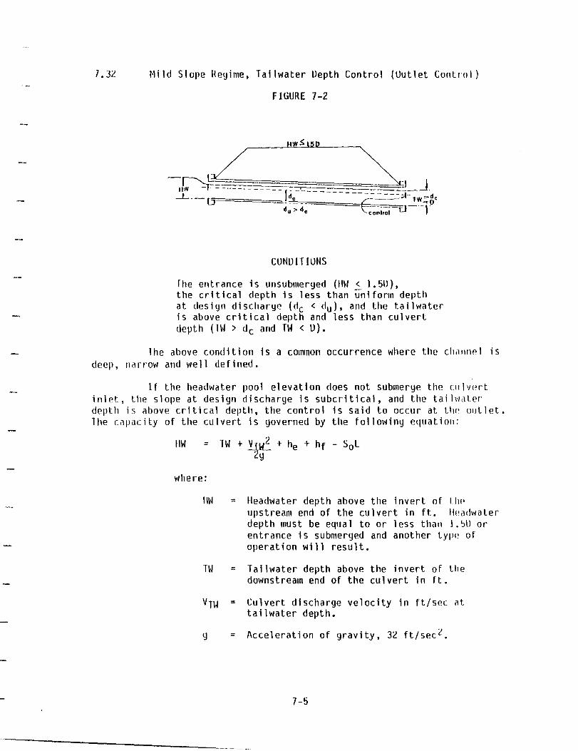
1.3'1.. Mild Slope Hegime, Tallwater Uepth Control (Uutlet Control)
FIGURE 7-2
IlW ~ l5P
CUNUlTlUNS
rhe entrance is unsubmerged (ItW < 1.5U), the critical depth is less than uniform depth at design discharge (dc < du ), and the tailwater is above critical depth and less than culvert depth (IW > d c and TW < U).
The above cond it ion is a common occurrence where the chilline lis deep, "arrow alld well defined.
If the headwater pool elevation does not submerge the clllv('rt inlet, tile slope at design discharge is subcritical, and the tailwdter depth is above critical depth, the control is said to occur at lhl' out let. The capacity of the culvert is governed by the following equation:
ItW = TW + ~J}i + he + hf - SoL 'l..g
where:
HW = Iteadwater depth above the invert of !.l,P upstream end of the culvert in ft. lif'iHlwater depth must be equal to or less than I.~IJ or entrance is submerged and another tYII!' of operation will result.
TIl = Tai lwater depth above the invert of the downstream end of the culvert in ft.
VTW = Culvert discharge velocity in ftlsec ~t tailwater depth.
Acceleration of gravity, 3'1.. ft/sec i .
7-5

he = Entrance head loss in ft.
he = Ke (VTW.t:. 2g
Ke = Entrance loss coefficient (see Table I-L).
hf Friction head loss in ft = SfL.
Sf = Friction slope or slope that wi II pnJtillu' tailwater depth equal to uniform depth.
So Slope of culvert in ft/ft.
L = Length of culvert in ft.
1.33 Steep Slope Kegime, Tai Iwater [nsigni ficant (Entrance Control).
FIGURE 7-3
d~d;= TW<SL -====-._.1-
L I CUNU IT IlJNS
The entrance may be submerged or unsubmeryed, the critical depth is greater than uniform depth at design discharge (dc > du ), and the tailwater depth is less than SoL (TW elevation < upstreal» flowl ine).
This condition is a cOl1lmon occurrence for culverts in rolling or hi Ily country. The control is critical depth at the entrance for 11~4 values up lu abuut 1.5U and entrance geometry for IlW values over about l.~lJ.
If critical flow occurs near the inlet, the culvert is <;(lid to have "inlet control." TIle maxil»um discharge through a culvert flowing part full occurs when flow is at critical depth for a given energy IlPild. To aSSllr!' lhat flow passes through critical depth near the inlet, lIl!? culvert IIIlIst be laid on a slope equal to or greater than critical slope for the desitjn discharge. The discharge is limited by the section near the inlet at ~Ihich critical flow occurs.
7-6

Ille headwater for a cul vert fl owi ng under tllese cond i t i OilS ~Ii til control at the inlet is determined from empirical curves in the fOllll of nOlllogrilphs (see Figures 7-11, 7-14, and 7-15).
7.34 "Slug" Flow Uperation (Uutlet/Entrance Control).
FWURE 7-4
HWiI!l.50
-.. r--- .... " uw '-..: ---_" l -- --. --':-
'i:J
.-u=~==~ =-=-= du
.!S.d;dc:-='====== TW <SUD
L
CUNUIT IONS
The entrance may be submerged or unsubmergell, critical depth is greater than uniform depth at design discharge (de> du ), and tailwater elevation is above critical deptl, at the entrance and helow the upstream soffit (SoL + de < TW < SoL + U).
fhls condition is typical of culverts located in roll inl) OJ'
mounlil i nOllS country. Control for thi s type of operation lIlay be at. t.hf' entrallce or the outlet or the control may migrate back and forth iletween the t~IO (hence, the name "slug" flow).
/Is the control lIlay shift from the entrance to the outlet., it Is reCOIIIIII(>nded that headwater be eva 1 uated for both s itual ions and thf~ hi yher value be used. Entrance control headwater may be determined frolll f'lIlpirical curves (see Section 7.52), and outlet control headwater evaluated by procedures outlined in Section 7.35 and/or 7.36.
7-7

1.j~ Mi ld Slope Hegime, Tailwater Greater Than Harrel Uepth (Uut let Control)
FIGUHE 7-5 HW'I! 1.50
1 ~-~ ~ Xi Tt~ ~.
[j L de -"du tJ
HWi!1.50
CUNO IT I UNS
Critical depth is less than uniform depth at design discharge (d c < du ) and tailwater is greater than culvert depth (rw > U), or critical depth in greater than uniform depth aldesiyn dlscllarge (dc > du ) and tailwater is above the upstream soffit (TW > SoL + U).
Most culverts flow with free outlet, but depending on t.1)I'o(jraphy, a tai 1I'lilter pool of a depth sufficient to submerge the outlet flIily forlll ilt some installations. For an outlet to be submerged, the depth at the outlet mllst 1)(' equal to or greater than the diameter of pipe or height of hox. The cilpacity of a culvert flowing full with a submerged outlet is governed by the following equation when the approach velocity is cOllsidered zero. Outlet velocity is based on full flow at the outlet.
where:
HW = Headwater depth in feet above the invl!rt of the upstream end of the culvert.
H = Head for culvert flowing full in ft.
= hv + he + h f
hv = Ve lac Hy head in feet based on fu 11 "O~I in cu 1 vert.
hv = V2 2g
= Friction head loss in ft = SfL.
7-U

he = Entrance head loss in ft.
TW = Tailwater depth in ft.
So = Slope of culvert in ft/ft.
L = Lenyth of culvert in ft.
7.36 Mild Slope Regime, Tailwater Less Than Barrel Ueptll (Uutlet Control)
FIGURE 7-6
HW>I~O
- .. I.;uu --(~uL====~~J -.1--u===='=O= -"-"'==-=:-F- ,Lo-
'or TW<de dc' 0
p·- 2-
du .. a~. ======1El-L _,-
torTW>de P·TW
CONUIT IONS
The entrance is submerged (HW ~ l.bU). The tailwater depth is less than culvert depth (rW < U).
Ihe capacity of a culvert flowing full with a partially suhllterged out 1 et is governed by the fall owi ng equati on when the approach ve I DC i ty j 5
considrred zero. Uutlet velocity is based on critical depthi f I~I depth is less than critical depth. If TW depth is greater than critical depth, outlet velocity is based on TW depth.
IIH =
~Ihere :
IIW Headwater depth in feet above the invprt of thp upstream end of the culvert. IIeadwatl'r dpplh mllst be greater than l.bU for entrance to be subilleryed.
II = IIead for culverts flowing full in ft (see Section 7.35).
7-9

P = Pressure line height in ft.
P = dc + D for TW < dc 2
P = TW for TW > dc
dc = Critical depth in ft. (see Figure l-l or 1-13).
0 = Diameter or height of structure in ft.
So Slope of culvert in ft/ft.
L = Length of culvert in ft.
7.4U END TREATMENTS
The normal functions of properly designed headwalls and {~ndw~ II 5 are to anchor the culvert to prevent movement, to control erosion and scour resulting from excessive velocities and turbulence, and to prevent adjacent soil fran sloughing into the waterway opening. All headwalls shall be constructed of reinforced concrete and may be either straight parallel headwalls, flared headwalls, or warped headwalls with or without aprons as may be rClluired by site cond it ions.
7.41 Conditions at Entrance
It is important to recognize that the operating characteristics of a culvert may be canpletely changed by the shape or condition at the inlet or erltrance. Uesign of culverts must involve consideration of eneryy losses that Inay occur at the entrance. The entrance head losses rnay be detenllined by the following equation:
= Ke V2 2g
where:
he = Entrance head loss in feet.
V = Velocity of flow in culvert in ft/sec.
Ke = Entrance loss coefficient (See Table 1-2) •
g = Acceleration of gravity. 32 ft/sec 2•
In general, the following guidelines should be used in tile selection of the type of headwall or endwalls.
7 -1U
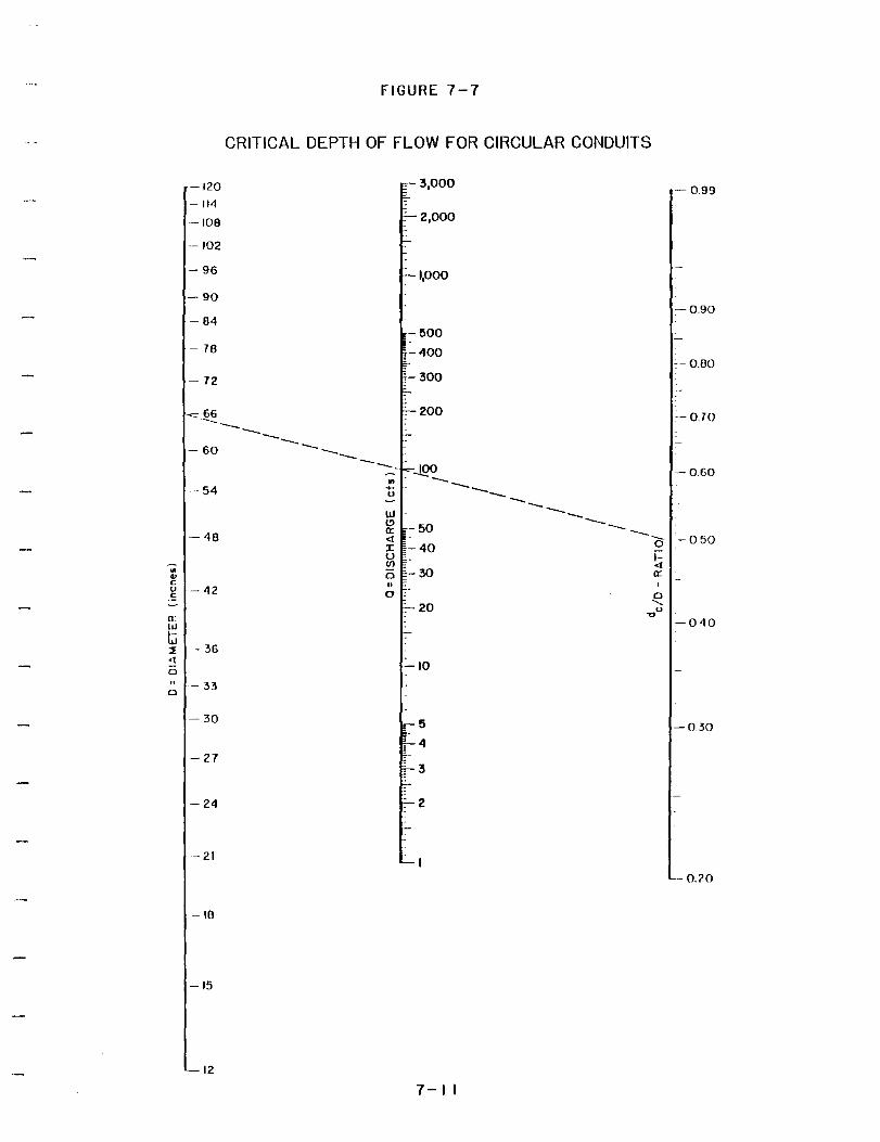
-; '" c 0 .!;
n: I<J
t;;
" <1 0
" 0
FIGURE 7-7
CRITICAL DEPTH OF FLOW FOR CIRCULAR CONDUITS
-120 -114
-108
-102
- 96
-90
- 84
- 78
- 72
""<0 .!i~ ----60 ----- 54
-48
- 42
- 36
- 33
-30
- 27
- 24
-21
-18
-15
12
. 3,000
1,000
- !l00
.-400
: 200
--::- . JQO .. ' -u ----__ w lE - 50 <I :r: u Ul o " o
-40
-30
: 20
-10
5
4
3
2
7-11
----------- -----o I-<I 0::
o ...... "'u
-0.99
-0.90
:- O.BO
:- 0.70
-0.60
-050
-030
0.20

~ -~ .ll l!J a: <t I U !!! 0
FIGURE 7-8
CRITICAL FLOW FOR BOX CULVERTS
de V ilL / e
CotmECT Q BVe READ W
CONNECT K B Vc READ ilL
-20
-30
-40
-50
-60
-70
-BO
-90
-100
-
-200
-500
-600
-700
-BOO
-900
-1000
2.0
1.9-
I.B-~ Z 1.7-~ -u iL 1.6-.,. ~ 1.5-u
tll4 -z <t ::13-z hl + 1.2-q
" '"
1.0
1=
'--r-
FRICTIONAL GRADE
ItWe'dcHtL
ItL'hy+h,
3
10
-15 lL -20 a -I -30 .... 0 =-40 i =-50
" :t: 100
7-12
-30
- 20
10 10-90-=
B.O B.O-=
=-60 1.0 .::
-5.0 6.0--
-4.0 15.0-
-3.0 4.0-0
3.0- ,-10
+l -2.0 : -90
~ If)
2.0-If) +' -BO_ o ~ " --' n
=-1.0 -0 I .-7.0 -<t =-O.B
r- >-w n. r-I - W
" 0 -so g -os .J .J 10- _l
I -0.5 <'10.90-= w - u - > -0.4 i= OBO: - 5.0 .J n: 0.70- <'I -0.3 ';;'o.SO-~ l)
0 - ~
'00.50- - 40 n: 0.2
u " 0.40-~
0.30--- 30
::: O.OB 0.20-
-0.05 -0.05
-0.04 -2.0
-0.03 010-
-0.02
0.01
--1.0

7.4~ Parallel Headwall and Endwall
1. Approach velocities are low (below 6 fps). 2. l3ackwater pools may he pennitted. 3. Approach channel is undefined. 4. Ample riuht-of-way or easement is available. S. Downstream channel protection is not required.
7.43 Flared Headwall and Endwall
1. Channel is well defined. 2. Approach velocities are between 6 and 1U fps. 3. Medium amounts of debris exist.
7.44 Warped Headwall and Endwall
1. Channel is well defined and concrete lined. ~. Approach velocities are between Hand 2U fps. 3. Medium amounts of debris exist.
Warped headwalls are effective with dropdown aprons to accelerate flow throuuh culverts, and warped endwalls are effective for transitioniny flow from closed conduit flow to open channel flow. This type of headwall should be used only where the drainage structure is large and right-of-~Iay or easement is 1 imited.
1.4~ Improved Inlets
Several types of improved inlets have been developed, illlt! the use of these inlets may provide sUbstantial savings by a reduction in the barrel size of tIle IJrOposed structure. Ijowever, the use of those inlets is optional and should be based on an economic analysis by the designer. For box culverts, reinforced concrete structures and structures usiny headwalls, the lise of beveled inlets or tapered inlets is strongly reco~nended. For nlore infonnation, the desiyner is referred to "Hydraulic Design of Improvements for Culverts," Hydraulic Engineering Circular No. 13, August, 1973 (a publication of the U.S. Bureau of Public Roads).
7.5U CULVERT DESIGN WITH STANDARD INLETS
The information and publications necessary to design culverts accordinu to the procedure given in this Section can be found in tIle "I~draulic Nanual" issued by the Texas Department of Highways and Public Transportation (Ref. I) and in publications of the Federal Highway Administratioll (Hefs. 2, 3, and 4). The uuidelines from these publications that cover the more cOll1l11on requirements are reflected in the nomographs at the end of this section. For special cases and larger sizes, the Federal Highway Administration publications should he used.
7-13

1.51 Culvert Sizing
The nomoyraphs in Figures 7-lJ through 7-14 can be used Itl calculate a series of curves which show the discharye capacity pel' h~rrel or per foot width of culvert in cfs for each of several sizes of s illli I ar type culverts for various Ileadwater depths in feet above the culvl','t illvert at the inlet. The invert of the culvert is defined as the low POillt of its cross section.
Culverts shall be selected based on hydraulic principles, economy of size and shape, and a resulting headwater depth that will not (,IIISe damage to adjacent property. It is essential to the proper desi':)l1 of a culvert that the conditions under which the culvert will operate dre known. The six types of operatiny conditions (already discussed in Sections 7.31 through 7.36 and represented in Figures 7-1 through 7-6) are:
1. Mild slope reyime, critical depth control (outlet control) 2. Mi ld slope regime, tailwater depth control (outlet control) 3. Steep slope regime, tailwater insignificant (entrance
control) 4. "Slug" flow operation (outlet/entrance control) !:>. Mild slope regime, tail water greater than barrel depth
(outlet control) 6. Mild slope regime, tailwater less than barrel depth (outlet
cant ro I)
The headwater depth given by the charts is actually til(>
difference in elevation between the culvert invert at the entrance alld the total head (that is, depth plus velocity head) for flow in the apprOdch channel. In most cases, the water surface upstream from the inlet is close to this level and the chart determination may be used as headwater depth for practical design purposes. Where the approach velocity is in excess of J.ll feet per second, the velocity head must be subtracted from the curve determination of headwater to obtain the actual headwater depth.
1.!:>2 Use Of Nomographs
The following procedure for culvert design requires the lise of nomographs, Figures 7-lJ through 7-14, developed for both inlet and outlet control.
1. List design data: Q(cfs), L(ft), invert elevations in and out (ft), allowable IlW (ft), mean and maximum flood velocities in natural stream (ft/sec), type culvert dnd entrance type for first selection.
2. Determine a trial size by assuminy a maximum averdlj{! velocity based on channel considerations to compute the area, A = Q/V.
/-14

3. Find flW for trial size culvert for inlet control anti outlet control. For inlet control, use Figure 7-1U, 1-13, or /-111. Next, compute the HW for outlet control with Figure 1-'], 1-11, or 7-12.
4. Compare the computed headwaters and use the hi gller II~I to determine if the culvert is under inlet or outlet control. If outlet control governs and the flW is unacceptat)t~, select a larger trial size and find another HW with the Ollt.il't control nomographs. Since the smaller size of culvl'l"t tlad been selected for allowable flW by the inlet control nomographs, the inlet control for the larger pipe Iwed not be checked.
7.6U DESIGN PROCEDURE
Due to problems arising from topography and other considerations, the actual design of a culvert installation is more difficult than the simple process of sizing culverts. The information in the procedure for design will be given as guidelines since the problems encountered are too varied and too numerous to be generalized. However, the design process presented should be followed to insure that some special problem is flot overlooked.
7.61 Des i gn Cornputat i on Forms
The use of a design computation form is a convenient method to obtain consistent designs with a minimum of culvert cost. An eXdllfple of such d fonn is Figure 7-15.
7.62 Invert Elevations
lIfter determining the allowable headwater elevation, tailwater elevation, and approximate length, invert elevations must be assuillerl. When considering ponded and non-ponded inlets, either for the design discharge or for sane lesser stonn that will not cause ponding, scour is not likely to occur in an artificial channel, such as a roadside ditch or a Illajor drainage channel, when the culvert has the same slope as the chanllel. To reduce the chance of failure due to scour, invert elevations corresponding to the natural grade should be used as a first trial. For natural chanrwls, the flow conditions in the channel upstream from the cuI vert should be investigated to determine if scour will occur.
7.63 Cu I vert Oi arneters
After the invert elevations have been assumed and using tile Design Computation Forms and the nomographs, the diameter of pipe that will meet the headwater requirements should be determined. The smallest diameter that appears in the nomographs and capacity charts is 1<' inches.
7-15

Since smaller diameter pipes are often closed by silt, it is reC(HIIIIH~llded that pipe slilaller than 1H inches not be used for any drainage wlH'r(' I.his manual applies. Since pipe roughness influences the culvert diallieter, both concrete and corrugated metal pipe should be considered in desiyrl, if they satisfy the headwater requirenents.
7.64 Limited Headwater
If there is insufficient headwater elevation to obtain tlH~ requireo discharge, it is necessary to either oversize the culvert barrel, lower the inlet invert, use an irregular cross section, or use any combination of the preceding.
If the inlet invert is lowered, special consideration 11111';1; be given to scour. The use of gabions, concrete drop structures, riprap. or headwalls with apron and toe walls should be evaluated to obtain tile proper desiyn.
7-16

- ~(J(JO
.. 4 (JOO
1000
eoo
600
400 >
~ 300 IJ1 "-U ~
L
Z - 200
a
lU
'-' 0::
" :c u 100 III 0 eo
L-60
50
30
20
-10
- 8
6
5
r w UJ .... ; x 0 III
W 0::
" :J a IJ1
"-0
z
FIGURE 7-9
OUTLET CONTROL NOMOGRAPH - HEAD FOR CONCRETE BOX CULVERTS FLOWING FULL,
n=0.012
12XI2
loxia 100r w
9 X9 eo w .... exe w
60 0::
" 1X 1 :J a en
aX6 ~
30 x 0 III
0::
20 " ..J :J
4X4 t!)
z "
~,,~,.~h~,.~~»~<~t~.~~~----!~,,-.-.~.,-__ ------~~
Sue~[AG£O OUTLET CULyEIH 'LOWING 'ULL HW· H. ha-lSo
'0' 0,,11.' ero .. " "01 lubm"9ld, cOrflpul1 HIN by "",hoU d',crib," 1ft ''''' ""HI" proclchui
l-ui 1" U.
~
I 0 -1
"I :c
- 4
5
- 6
- 8
- 1.0
- 2
3
- 4 o 15X:l5 r
U III W Z 0:: w 3X 3 ~
u.. a 0
0
25X2.5 6
2X2
r
- 5
- 6
---1·-~.TS l~a
~ 10
'" L 20 ! ~
CI
! z 0: ~ ~
7-17

tUJ UJ LL
~- 12
- 11
- 10
- 9
8
- r
- 6
- 5
Z - 4
o
)(
o ([]
lL o f- - 3 :t: to
UJ :I:
FIGURE 7- I 0
INLET CONTROL NOMOGRAPH HEADWATEr~ DE P T H FOR BOX C U L V E R T S WIT H IN LET CON TrW L
600
500
- 400
300
200
b - 100 o lL 80
60
z 40
co 2: _ 30 a
( I ) ( 2) ( 3)
EXAMPLE 5'11 2:' 80" o I 7~ ct.
alNs . I!! chin
Inl,t Hr Hr -0 ,.,t
.-8 - 9 .- 10
~7~_ - 8 - ---- ---- 7 - 8
- 6 - 6 - 7
-5 - 6 111 1.7, ) , - 5
121 1.90 J~8 - 4 - 5
131 2.0~ 4. I - 4 ~ ~~-~-- ..-~~- --
- 4 - 3
- 3 - 3
o 1 i=~--2 - ~-2-- .--
-- - 2
- 1.5
- 1.5 - 1.5
/t-
/' ~ /' w
:I: \. / lL r~-- '---
~'';/ 0 \.~~-
./ 20/
Ul
" a: ~ - 1.0
lL o o
/'
10
8
6
5
t- - 4 ct II:
-3
ln,1I 01 wln, •• 11 "are
Hlr o SCALE
III
121
131
WINGWALL FLARE
30· '0 15-
90· 'nd l!i-
O· ... ',n,lo", 0' I,d .. ,
h ... leal' (U or (l) prOI_c' harho",,'" 'e tul, fI', thin IIU ,Iralthl Inclined lint Ihrotlth o ond a .ealll, at ' ... fli ..
IIIUltrahd.
z . ---~ -~-- f----.9 -1.0 -10
:t: t-
.9 o. ~ -.8
- .9
0: w f- ~.7 <t 3' a ~
- .7 - .7 <t w :I: f- .6
~
- .5
-.5 -.5
-----1---- .4
- .4 - .4
~I,--- -----
'-- .30 .35 .35
7-18

<II
"-'-' ~
0
UJ to a: <I I '-' Vl
e
FIGURE 7- I I
OUTLET CONTROL NOMOGRAPH - HEAD FOR
CONCRETE PIPE CULVERT FLOWING FULL,
n= 0.0 I 2
-2000
- 1000
-- 800 120
- 600 108
- 500 96
'. ~~~~,,~»~~~,~.,~t~',%~"~----S~'.-'-'~S.-__ ------~~~ .. = " , ... ,
SUBMERQED ouTLET CULvERT FLOWING FULL HW' H' ho-LSo
Fot "11"" ero_,. '"" • ..,bm"v,d, COrnetu" HW by ",.thod, .... cub.tI i" 'he 4"'9" ",ocadu,.
-- 4
- 5
- 6
- 8
,. ".q -10
- 400 84
- 300 72
66
- 200
54
<11
'" :J: '-' -100 '!: 42
·0 /" 0':-" Z
80.-- -
0 36 -- 60 a: 33
'" - 50 f--
'" - 40
::2 <I (5 27
- 30 24
21 - 20
18
-10 -15
- 8
- 6 12·
- 5
4
.,0 LillO -- -- --It.~O,5 -;'0°
7-19
.,00 • f •• •• 0
o to \1'
f--- r~ 2 II'
'"~ IL
1- 3
z
I I-
e [- 4
., UJ I I
1- 5
- 6
- 8
-10

FIGURE 7- I 2
OUTLET CONTROL NOMOGRAPH - HEAD FOR STANDfl.IW
C. M. PIPE CULVERTS FLOWING FULL, n=O.024
-2000
- 1000
-800
-600
- 500
-400
-300
:- 200
ttl \, -u'
~ -100
z (} - 80
w' 60 C> -Q: <I - ~O J:
In w l: u ~
~
0
~-40 Ct: O.3~ til
O' -- ---,--_ 30 w
:e <I o
- 20
-10
- 8
- 6
- ~
- 4
- 3
" z z a: " '-
-120
-108
- 96
- 84
- 72
- 66
- 60
-~4
- 48
-42
- 36
-33
-24
- 2 I
- I 8
- I ~
- I a
w z J
--~j ---L--7 =-~ ---l:="~ --r:~-~~-"""'~~~ SloP' so- ~ri,~,,=~
4
·6 SUBMERGED outLET ~ULYE"T FLOWING FULL
IIWo .. H + ho + EI. Outlat Invert .0
-10
<<' 1- ,-e;> ....
-s- hi 2 III
'< ". './
~ Z
'" :r: - 3 ~ ....
0 .~
w - 4 :r:
- ~
·6
- B
- 10
-·20
7-20

U)
W 1: u Z
z
0
~ n: w > ...J ~ U
lL 0
n: '" .-w ::I <I (]
FIGURE 7-13
INLET CONTROL NOMOGRAPH - HEADWATER DEPTH FOR
CONCRETE PIPE CULVERTS WITH INLET CONTROL
10 () - 10,000
- 8,000 EXAMPLE ( I ) (2) (3) - 6.
I ~ G . - 6,000 O. AI, Inch •• U.5 ''''I 6 . O/N.120d,
144 - !I,OOO - !I,
- 4,000 !!.t II, r 6. - !I.
132 D r .. t - 5,000 - !S. - 4.
III t.S •• 4. - 120
If! 2.1 7.4 - 2,000
lSI t.t 7. f -. f-4.- 1 _______
- 108 - 5. -0 1ft r .. , 5.
- 96 1,000 - 3. -
- 800 .-~
~ - - ----
- 84 ---_ .. -=-- 2. ----- 600 /- 2: .
- !lOa /'
// . D - 2 .
12 - 400 / ..... f\.V I
300 III - i-~ - I. !I .. I. 5
"" ~ .. u ",/ III
n: 60 ~ ,- 200 '" w - 1.5 / ~-
/ w 54 Z ./ ~
CI /" <I (]
, / w - 100
- 48 / CJ - ~
n: - 80 ,/ <I 1: ----
l: ~
, 42 u - 60 0_ - 1.0 - 1.0 w
III - 50 II, ENTRANCE 0 (] SCALE - 1.0
- 40 0 TYPE n: w - .9
38 f- - .9 - :- 30 (II S.url ,dO' .lIh <I flud •• U ~ - ,9
33 0 ---:- 20 121 GreG" •• n4 .11" <I
w - .8 30
1'. .. d •• 11 :I: - .8
1" GrOut .nd - ,8
21 proJecth,.
- 10 - .1 - ---- ~_.7_.
- 24 - 8 - ,7
- 6 To u .. teah 12' Of 13, I',o)le'
21 - 5 ho,ho"'oll, I. Hoh fl" thtn
- 4 u ... holthl Inclln." II", th,euth D ond Q IClllln, or U",'" II - .8 .6
.- 3 IIIutlrol,d. - ,6
18
2
I!I L .!I - .!I
- 1.0 - .!I
- 12
7-21

III "J OJ: ()
z
~
Cl
,-n: w -. :, =J l)
u. 0
n: "J ,. 10' ::! <t
0 ~
" 0 n ., 0 z ., , on
FIGURE 7- I 4
INLET CONTROL NOMOGRAPH - HEADWATEH DEPT"
FOR C. M. PIPE CUL VERTS WITH INLE T CONIIWL
. 160 - - - 10,000 ( I )
168 - B,OOO EXAMPLE
·156 ·6.000 0- ~6 Inch .. IS.O I .. ., -- 6. ( I' )
- 5.000 OIN,,, ,I.
144 - ~,OOO - 5. 6. !!J. II,
. 132 3,000 0 ,r .. l)
2 ~'--u '" 1.0 '.4 -=-->1-. _.
120 121 Z .' o. , .... -- 2,000 ... 4 . .. '" 1.1 6.1 - 106 -' 3 . ..
-' °0 'n ".t .. 96
.. .,000 3 . :J ,-u 800 :> 0: ...
04 VI 600 2. 500
400 /' 2.
12 /" III 300 k /'/ 1.0 U /
/' ~ 200 ,,,to,/'
- 60 I 5
Z \.i-~" ... ,
a ,./ ,. 54 " "J /' :;,:. -- -_._--
I<J 100 / <t Cl = BO/ - 4 B 0:: Cl
<I /
:r: "-/u - 60 - '.0 T- 10
- 42 /' (/) - 50 / a ~.
n. ../ - 40 '" n -:-:-9-- -g-
/36 30 II, ENTRANCE n: 0 SCALE ,01
TYPE , .. H <I
20 III H.a,_.,11 ~ - .8 .8 0
- 30 err MI,u" hi "1'1"''" . ( '" I •• I.p. I
21 - 10 1" 'to lit tI". .1 .1
B 24
6 - 5
10 u" leolt U, .r 13) project 21 - 4 horhonhll, 10 ItO" (I), ''''" - .6
.... I,olthl '"clin,d lin, Huout" .6 - 3 o 0'" 0 .eol." ,f , .... f ••••
18 lIIu.t .......
;- 2
- 15
1.0
_. '2
7-22
(3)
·6.
~.
4.
3.
2.
I.~
.--
. '0
.9
.8
.1
.6
- .5

-.j
I N VI
PROJECT: DESIGNER:
DATE:
HYDROLOGiC AND CHANNEL INFORM:' TION SKETCH STATION:
1.-=7 ~ -.l 0 1 = TAILWATER ELEVATION = __ i T .. O2 = TAILWATER ELEVATION = __ -=r-T: EL.:Jt-EL. L == (0 1 : DESIGN DISCHARG E, SAY 025 ) MEAN STREt."c VELOCITY = ....b... =
02: CHECK DISCHARGE, SAY 050 OR 0100 MAX. STREAM VELOCITY = 100, --
HEADWATER COMPUTATION ; >-CULVERT oJ .....
oJ .. -DESCRIPTION SIZE INLETCONT. OUTLET CONTROL HW = H + no - L. CHART o • .. (J COST COMMENTS Q
~ :c ... 0
dc+O " oJ Hw iw Hw NQ. H .. Z o w IENTRANCE TTPEl 0- H .. K. H de -2- no L. 0 :>
(J
I
I
I I I I I I
SUMM':'RY & RECOMENDAT1ONS:
0 fTl (J)
G)
Z ."
0 " 0 c s: ::0
""C fTI C -.j -l I ::t> -l 01
0 Z ""1'1 0 ::0 s:
I

SECTION 8 - BRIDGES
8.10 GENERAL
When it has been determined that a bridge will be placed at a stream crossing, the following procedures will be used to hydraulically design the bridge, unless the County Commissioners determines that a more detailed analysis shall be done. All bridges shall be designed to pass a 100-year frequency storm event with no more than one foot of head loss.
It should be noted that columns, piers, etc., will not be considered in the following discussions. Usually, they can be neglected. However, their effect in reducing the waterway opening should not be neglected if they constitute a substantial cross-sectional area themselves. This is particularly true in the case of skewed crossings with normal bents.
Throughout the discussions of bridge design, it is assumed that normal cross sections and lengths are used; that is, cross sections and lengths which are perpendicular to the direction of stream flow at flood stage. If the crossing is skewed to the stream flow at flood stage, all cross sections and lengths should be normalized before proceeding with bridge length design. If the skew is severe and the floodplain is wide, elevations in the normalized section may need to be adjusted to offset the effects of elevation changes in the point displacement between the skewed section and the normalized section.
Often structural and other considerations will cause a bridge opening to be larger than the bridge opening required by hydraulic design. For instance, a header might be placed in a certain location due to soil instability, or bridge costs might be cheaper than embankment costs, or a fixed grade line might dictate an excessive freeboard allowance. These and others are valid considerations that affect bridge waterway openings; however, hydraulic computations are necessary in order to predict the operation of the waterway opening at flood stages. Hydraulic design is not to be neglected, and reasons should be noted for any specified opening in excess of that determined by hydraulic design.
8.20 TERMINOLOGY
Design Highwater Elevation - A calculated water surface elevation in the natural channel for the design discharge. This is the elevation that is the basis for all bridge length calculations.
Backwater - Depth of water that ponds above the design highwater elevation in order to force the design discharge through a restricted opening. This term is used primarily for bridge span type structures (see Figure 8-3).
8-1

Conveyance (K) - Carrying capacity based on the MallflillU (''IllatiOIl of a specific cross section or portion thereof as defirH'd by:
K = 1.4U6 AR 2/3 ---n
Natural streal" conveyance - The sum of all subsection CIJIlveyallces throlluhotJt a cross section of the natural stream for a speci fic hiuh~later elevation. Structure conveyance is the sum 01 1I1P
conveyances for each individual opening for a specific Iri,)ilwat.er elevation. The two conveyances (natural K and structurp K) IIlIlst be designated to keep them separate, because they are not: to be related to each other.
Freeboard - That clearance between water surface elevation ilfld low superstructure. A minimum freeboard of 2 feet abovl' observed highwater or design highwater, whichever is greater, shall be used.
1.l.3U FLOW nmOUGI1 BR lOGES
Compared to culvert flows, flow through bridge openinus 'I'quires that more emphasis he put on viewing the entire pattern of flow ill the floodplain, especially the flow approaching the bridue (or brid~J!'s). lllis is necessary because tile relationship of floodplain width to opl!nilll) width is more complex than for the usual culvert opening (see Figure U-l).
FIGURE I.l-l
PATTEI!N UF FLUW TI1ROUGH IlRlUGE UPENINliS
U-2

When flood flow encounters a restriction in the natural stream, certain natural adjustments take place in the vicinity of the restriction. That portion of the flow not directly approaching the bridge opening has no convenient way to continue downstream. The flow, therefore, will pond until sufficient head is built up to force it to turn toward the bridge, and generally move parallel to the highway embankment. As the flow moves toward the bridge opening, the velocity increases above the natural floodplain velocity. This increased velocity can cause scour, sometimes severe, along the highway embankment and particularly at the bridge header. At the header, the intersecting velocity vectors cause high turbulence and eddies that often result in the failure of an interior bent near this turbulence (see Figure 8-2). If there is only a single structure, the flow will find its way to the single structure. If two or more structures are available, the flow, after accumulating a head, will divide and flow to the structure offering the least resistance. This point of division is called a flow divide.
In usual practice, it is recommended that the flood discharge be forced to flow parallel to the highway embankment for no more than 600 to 800 feet. If flow distances along the embankment are greater than recommended, then a relief structure to provide additional opening should be investigated, or a spur dike is recommended to control the turbulence at the header. Also, natural vegetation remaining between the toe of the slope and the right-of-way line is advantageous in controlling flow along the embankment.
Multiple structures and spur dikes are discussed in Sections 8.50 and 8.60.
The backwater effect caused by the constriction in the natural stream is depicted in Figure 8-3, and pertinent design considerations are given in Section 8.40.
The waterway opening defined by design highwater, the left and right header slopes, and the natural ground profile (or proposed through-bridge channel section) should be such as to cause an average through-bridge velocity of from 4 to 6 feet per second. This can be accomplished by simply moving the header slopes nearer together or farther apart as necessary. Average through-bridge velocities higher than 6 feet per second must be approved by the County Commissioners.
The average through-bridge velocity used throughout this chapter is calculated by the formula:
v = Q/A
where:
v = Average velocity in ft/sec.
A = Normal cross-sectional area of the water in ft2.
Q = Design discharge in ft 3/sec.
8-3
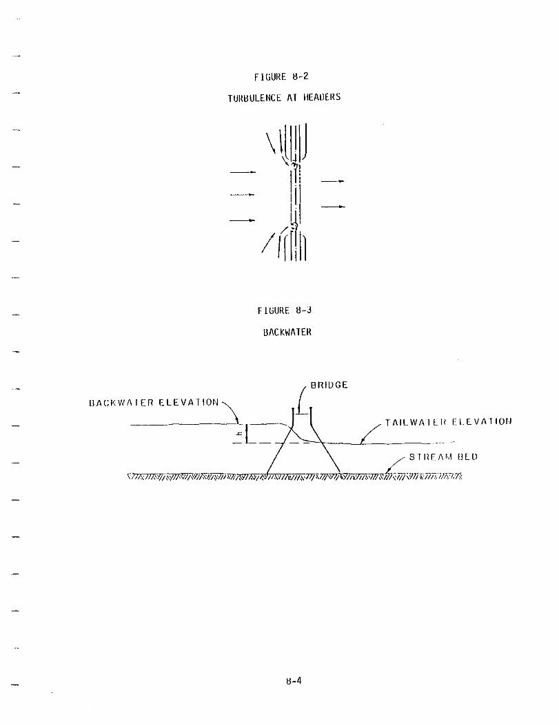
UACI<W/\ I En
FIllUHE H-2
TUIWULENCE AT IIEAUEHS
-
F 1 (lUHE 13-3
I3ACKWATEH
ELEVATION \
~[-
H-4
/ TAILWA_:~II ~:L[Vl\r lor~

H.4U SINGLE STRUCTURE
"Single structure" refers to the crossing of a floodplain ~Ihich re1luires only one opening in the highway embankment.
The following is the recommended procedure (Ref. 7) for establishing a single structure length and elevation of low superstructure after ohtaining an accurate cross section and determining the desiYl1 highwater elevation.
Step 1. Assume average trial through-bridge Velocity (V t ) that is less than the maximum allowable velocity and more than 4 fps.
Step 2. Find water cross-sectional area (At) required for trial velocity.
Step 3. Estimate average depth of water (Dt) in cross sections.
Step 4. Find approximate trial length (L t ) of waterway ollening.
Step 5. Position headers in stream cross section so thdt tlley average approximately Lt feet apart.
Step 6. Find exact waterway area (A) below design hiyllVIater within structure limits.
Step 7. Find average through-bridge velocity (Vstruct) for the actual waterway area.
Vstruct = Q/A
Step H. If Vstruct is greater than 4 fps and less than b fps, the bridge length sizing is complete. This lelHJth can usually be adjusted sl ightly to fit span length requirements.
If Vstruct is not greater than 4 fps and less thiln 6 fps, the length should be adjusted as necessary and the process returns to Step 5. This routine should be repeated as often as necessary unti I average through-bridge velocity is within the prescrii>l>tI ve I oc ity range.
Step Y. The low steel or low concrete of the structure Sllould be placed at an elevation that provides at least 2 feet of freeboard over the des i gn hi ghwater. Often, ')ollle observed highwater exceeds the design highwater. In this case, it is usual practice to clear the hiyher of the highwaters. In any event, the design highwater should be used in the bridge length determination.
8-5

Step 10. The backwater caused by the constriction of til£' bridge opening should be approximated by the followiny formula.
h = Vs trllct 2 - V2 2g
where:
h = Increase in depth over desiyn highwater in ft.
Vstruct = Average through-bridge vel aci ty.
V Average ullrestricted ndLul"dl stream velocity in ft/sec.
g = Acceleration of gravity, Jl' ft/sec 2•
8.5U MULTIPLE STRUCTURES
Uue to a relatively wide floodplain or multiple discharljP cOllcelltrations (as opposed to a single concentration), it may be npcessary to design multiple openings. This is usually referred to as a main channel bridge with relief openings. This type of crossing simply providps openings at or near the flow concentrations so as to reduce a I ong- embankment fl ow and reduce backwater efr ects.
Multiple structures should be designed so that their J'elative carryiny capacities (or structure conveyances) match the predictpli relative discharyes approaching them. This is necessary because each bridye must have the capacity to carry its share of the discharge. Otherwise, those bridges whose capacity is less than necessary will be overloaded with resul tant high velocities and, in effect, will cause a reapportionment of the approach discharges. This, in turn, will cause high backwaters and hiyh along-embankment velocities. In addition to making this balance in proportion, the designer must satisfy average through-bridge velocity requirements.
8.~1 Flow Uistribution
AFter determination of the design highwater at a multiple structure location, it is still necessary to determine just how the flovi divides itself across the floodplain at flood stage. If the flow liivides, as in the case of multiple structures, determine the portion of the total flood discharge that will be carried by each structure as previously stated in Section 8.3U.
8-6

One of the best methods for accomplishing this is by actuill observation of the flow at design discharge and highwater at the IJrOposed site. However, it is rare that the engineer is able to make such an observation when the proper set of circumstances occurs. Therefore, the following method has been devised for determining flow distribution and establishing flow divides (Ref. 7).
Inspection of incremental discharges or conveyances across a floodplain cross section usually reveals where the relatively heavier concentrations of flow are located. By determining these heavier concentrations of flow, the engineer usually can decide the proper locat ions for each of the bridges. The most strai ghtforward method of spotting these heavy concentrations of flow is by use of a cumulative conveyance (or discharge) curve. This curve is constructed as follows:
Step 1. Apply the design highwater to a natural strealll cross section in the immediate Vicinity of the proposed design section. The section chosen for this highwater appl ication should be a typical section which ~Ii II definitely control the flow distribution in tile reach of the stream wherein the structure is located.
Step 2. Calculate cumulative natural conveyances for eacll subarea across the sect i on from I eft bank to r i qht bank (Figure B-4). (Uischarges may be calculated, bllt all this requires is multiplication of conveyances by the square root of the stream slope. This is an I~xlril step and nothing is actually gained by it since the final shape of the curves would be the same.)
Step 3. These cumulative natural conveyance values are plotted versus the cross-sectional stationing creating il curve as shown in Figure 8-4; the value of the last plot is equal to the total conveyance of the stre~" section.
Step 4. By inspection of this curve, it is seen that, in the vicinity of points I, 2, and 3, the slope of the curve is relatively steep. This is caused by a rapid increase in natural conveyance with respect to distance across the section. These points define the approxililate best locations for bridges. The points on the curve where the curve has the fl attest slopes defi ne the approximate locations of flow divides.
That portion of the design discharge carried between th(! flow divides should be determined by direct calculation or by proportion of relative natural conveyances (Figure 8-4). At this point, the relative discharges have been detennined.
13-7

~ 1 'J U C o :> OJ :> c ,.,
U OJ .~
o
" E Cl
u
o
FIGURE 8-4
CUMULATIVE CUNVEYANCE CURVE
Colculaled
C ross Sec lion
rlow Dlvlde--~I
5100 10100 15100 20100 Sialioning
U.5~ Design Uf Multiple Structures
/
CUMULATIVE COfJVEYANCE cunvr:
(flow divides, hriri'lP lo[olions,
Individual disch'"ges)
1- 1------ I 25100 30'00 35100 40'00
The design procedure (Ref. 7) to be followed in establishing the size of multiple waterways is outlined below. llu is the design discharge and sUiJscripts I, ~, and 3 refer to left floodplain, main channel. ilnd right floodplain, respectively. This example makes use of 3 bridyps. lIowf'ver, there may be more than 3 bridges or only 2 bridges. 111£' procedUre is the same in any case.
Step 1. Using 4 fps as mlnlfllum allowable velocity and IJ fps as a maximum allowable velocity, determine the approximate average velocity (VU) of all 3 openings.
Step 2. Uetermine approximate total waterway opening, II\).
AU = llo/VlJ
[HI

Step 3. Determine approximate waterway openi ng (Ai) for bridge I. bridge 2. and bridge 3.
Al = !ll x AD Qo
A2 = 92 x AD QO
A3 = .Q3. x AD QO
Step 4. With AI. A2. and A3. and assuming average water depths (01. 02. and 03). determine approximate structure lengths (L1. L2. and L3)'
Ll = ~. etc. 01
Step 5. Determine structure conveyances K1. K2. and KJ •
Ki = 1.486 AR2/3 n
Neglecting the constant 1.4H6. a relative convrYJI1Ce factor to be used in apportioning the total fI(M between openings is
In the case where under-bridge terrain is expected to be similar for each bridge. "n" is constant and relative conveyances may be evaluated as
then Kr = Kl + K2 + K3' If the values Kl/KT. K2/KT. and K3/KT are approximately equal to Ql/QO. Q2/UU. and Q3/GO. respectively. the structure conveyances are said to be balanced. Otherwise. adjustments in individual bridge lellgths should be made in order to effect this balance of proportions.
Step 6. Oetermi ne vel oci ty requi rements that must be IIIl't in addition to the proportion balancing of conveYdnces. With the trial waterway openings. the velocity requirements should be checked. Approximate velocity
8-9

throuyh each structure (Vstruct = Q/A) should hI' not 1 ess than 4 fps or greater than 6 fps. Note thilt a change in one or more bridge lenyths affects til!! lotal conveyance. Therefore, any change made should Ill'
accompanied by recalculation of relative structllre conveyances.
Step 7. lJetermine backwater head approximated by the fOJ'lllul a:
h = VJ2 - V22 2g
where:
Vl = Average throuyh-bridge velocity for all openings in ft.
V2 = Approach velocity in natural stream in ft/sec.
g = Acceleration of gravity, 32 ft/sec 2•
H.6U SPUR DIKES
Spur dikes are beneficial at sites where the travel along the embankment is in excess of 6UU feet. advantayeous for improving the characteristics of flow structure.
distance of tile flow Spur dikes are also throuyh a sinyle
Spur dikes have the advantaye of initi al economy and the fact that they are convenient and inexpensive to maintain. They functiorl by directiny along-embankment flow out away from the bridge openiny. This causes any parallel-embankment velocity to be removed from the embankment itself and serves to greatly reduce the under-bridge turbulence usually caused by intersecting flow vectors. If scour is still a problem, the end of the spur dike is eroded and not the bridge header. Figure U-5 shows the recoillmended geometry of spur di kes and affected stream flow. The top of spur dike elevation should be above design highwater elevation a Illinilnum of 2 feet. Also, it is reconunended that natural vegetation be left around the end of the spur dike.
H-IO
FlliUHE H-!>
SI'UH U I KE
H-ll
1.
2.
3.
4.
5.
6.
7.
8.
9.
10.
11.
12.
13.
14.
15.
16.
17.
REFERENCES
City of Austin, Engineering Department et al, Drainage Criteria Manual, Austin, Texas, 1977.
Federal Highway Administration, Hydraulic Charts for the Selection of Highway Culverts, USGPO, Washington, D.C., 1965.
Federal Highway Administration, capacit~ Charts for the Hydraulic Design of Highway Culverts, USGPO, Wash ngton, b.c., 1965.
Federal Highway Administration, Hydraulic Design of Improved Inlets for Culverts, USGPO, Washington, D.C., 1972.
u.S. Weather Bureau, Rainfall IntensitY-Duration-Frequency Curves, Technical Paper No. 25, Supt. of Doc., Washington, D.C., Dec. 1955.
u.S. Weather Bureau, Rainfall Frequency Atlas of the United States, Technical Paper No. 40, Supt. of Doc., Washington, D.C., May 1961.
Texas Department of Highways and Public Transportation, Bridge Division, Hydraulic Manual, Third Ed., December, 1985.
City of Waco, Engineering Department, Storm Drainage Design Manual, Waco, Texas, 1959.
Chow, V. T., Handbook of Applied Hydrology, McGraw-Hill, New York, 1964.
Chow, V. T., Open Channel Hydraulics, McGraw-Hill, New York, 1959.
King, H.W., Handbook of Hydraulics, Fourth Ed., McGraw-Hill, New York, 1959.
u.S. Geological Survey, Techniques for Estimating the Ma~nitude and Frequency of Floods In Texas, Water Resources Investigatlons 77-110, Open-File Report, 1977.
Portland Cement Association, Design and Construction of Concrete Sewers, Portland Cement Association, Skokie, Illinois, 1968.
Portland Cement Association, Handbook of Concrete Culvert Pipe Hydraulics, Portland Cement Association, Chicago, Illinois, 1964.
Bauer, W.J. and Woo, Hydraulic Design of Depressed Curb-Opening Inlets, Highway Research Board Record No. 58, Washington, D.C., 1964.
Federal Highway Administration, Drainage of Highway Pavements, Hydraulic Engineering Circular No. 12, 1969.
Izzard, Carl F., Simplified Method for Design of Curb-Opening Inlets, Annual Meeting of the National Transportation Board, January, 1977.

18. Karaki, S.S. and Haynie, R.M., Depressed Curb-Opening Inlets Experimental Data, Colorado State University, Civil Engineering Section, Fort Collins, Colorado, 1961, CER61SSK34.
19. National Research Council, Building Research Advisory Board, A Study of Invert Crown Residential Streets and Alleys, Federal Housing Admlnlstratlon, Washlngton, D.C., 1957.
20. Oglesby, H., and Hewes, I., Highway Engineering, John Wiley and Sons, New York, 1954.
21. Searcy, J.K., Design of Roadside Drainage Channels, U.S. Bureau of Public Roads, Hydraulic Design Series No. 4, USGPO, Washington, D.C., 1965.
22. Linsey, K.; Kohler, M.A.; and Paulhus, J.L.H., Hydrology for Engineers, Second Ed., McGraw-Hill, New York, 1965.
23. Schulz, E.F., Problems in Applied Hydrology, Water Resources Publications, Fort Collins, Colorado, 1974.
24. Soil Conservation Service, SCS National Engineering Handbook, Section 4, Hydrology, U.S. Department of Agriculture, August, 1972.
25. Soil Conservation Service, Urban Hydrology for Small Watersheds, Technical Release No. 55, U.S. Department of Agriculture, 1975.
26. City of Omaha, Omaha Metropolitan Area Stormwater Management Design Manual, Omaha, Nebraska, 1980.