arX

iv:1

402.

3591

v2 [

astr

o-ph

.HE

] 1

9 Fe

b 20

14

Draft version December 18, 2017Preprint typeset using LATEX style emulateapj v. 08/22/09

THE HARD X-RAY PERSPECTIVE ON THE SOFT X-RAY EXCESS

Ranjan V. Vasudevan1,*, Richard F. Mushotzky1,2, Christopher S. Reynolds1,2

Andrew C. Fabian3, Anne M. Lohfink1, Abderahmen Zoghbi1,2, Luigi C. Gallo4, Dominic Walton5

Draft version December 18, 2017

ABSTRACT

The X-ray spectra of many active galactic nuclei (AGN) exhibit a ‘soft excess’ below 1 keV, whosephysical origin remains unclear. Diverse models have been suggested to account for it, includingionised reflection of X-rays from the inner part of the accretion disc, ionised winds/absorbers, andComptonisation. The ionised reflection model suggests a natural link between the prominence of thesoft excess and the Compton reflection hump strength above 10 keV, but it has not been clear whathard X-ray signatures, if any, are expected from the other soft X-ray candidate models. Additionally, ithas not been possible up until recently to obtain high-quality simultaneous measurements of both softand hard X-ray emission necessary to distinguish these models, but upcoming joint XMM-NuSTARprogrammes provide precisely this opportunity. In this paper, we present an extensive analysis ofsimulations of XMM+NuSTAR observations, using two candidate soft excess models as inputs, todetermine whether such campaigns can disambiguate between them by using hard and soft X-rayobservations in tandem. The simulated spectra are fit with the simplest “observer’s model” of ablack body and neutral reflection to characterise the strength of the soft and hard excesses. A plotof the strength of the hard excess against the soft excess strength provides a diagnostic plot whichallows the soft excess production mechanism to be determined in individual sources and samples usingcurrent state-of-the-art and next generation hard X-ray enabled observatories. This approach can bestraightforwardly extended to other candidate models for the soft excess.Subject headings:

1. INTRODUCTION

Matter accreting onto supermassive black holes pro-duces emission from radio–to–X-ray energies, with a va-riety of different physical processes being relevant in eachband. The direct luminous thermal power output fromthe central accretion disc appears in the optical–UVregime; a corona of electrons above the accretion discCompton up-scatters this radiation to produce a power-law X-ray tail extending to hundreds of keV or greaterdepending on the coronal temperature. This ensemble isoften shrouded by dust and gas which introduces absorp-tion features including a low-energy fall-off from photo-electric absorption, and troughs/edges from ionised ab-sorption. Fall-offs are observed at higher energies due toCompton-scattering, and X-ray reflection from the ac-cretion disc can reprocess coronal emission to produce adistinctive set of continuum features, including a reflec-tion hump peaking at 30 keV and a broad Iron line at ornear 6.4 keV.Many AGN exhibit an excess at soft X-ray energies

(. 2 keV) over the coronal power-law. This was firstnoticed by Holt et al. (1980) and Pravdo et al. (1981),and more definitively confirmed with broad-band obser-

1 Department of Astronomy, University of Maryland, CollegePark, MD 20742-2421

2 Joint Space-Science Institute (JSI), College Park, MD 20742-2421

3 Institute of Astronomy, Madingley Road, Cambridge, CB30HA, UK

4 Department of Astronomy and Physics, Saint Mary’s Univer-sity, 923 Robie Street, Halifax, Nova Scotia, B3H 3C3, Canada

5 Cahill Centre for Astronomy and Astrophysics, California In-stitute of Technology, Pasadena, CA 91125

* ranjan@astro.umd.edu

vations by Singh et al. (1985) and Arnaud et al. (1985).The feature can be modelled as a black body with analmost universal effective temperature of ∼0.1–0.2 keV.The physics of this feature remains uncertain, despite itcontributing a potentially significant fraction of the totalluminous power output of AGN. The small range of effec-tive temperatures observed disfavours a scenario whereit represents the hard tail of the accretion disc spec-trum peaking in the far-UV (e.g., Miniutti et al. 2009;Ponti et al. 2010), as sources with different masses andaccretion rates would be expected to exhibit soft excesseswith different temperatures. Instead, atomic process areoften invoked to explain the soft excess, whereby a se-ries of lines are smeared together to produce the fea-ture. Two mechanisms can be invoked here: 1) ionisedreflection with light bending, in which the series of softX-ray lines are relativistically blurred due to being pro-duced very close to the centre of the accretion flowof a rapidly-spinning black hole (Ross & Fabian 2005;Crummy et al. 2006; Walton et al. 2013), or 2) ionisedabsorption, where the soft excess is not really an ‘excess’at all, but the remnants of the true power law at lowenergies, with the high energy power-law being absorbedby smeared, ionised absorption with very high cloud ve-locities (Gierlinski & Done 2004).Both models produce statistically acceptable fits

to XMM data for the same set of PG quasars(Middleton et al. 2007, Crummy et al. 2006), but bothrequired strong relativistic smearing of either the emis-sion or absorption features. Schurch & Done (2008)found that this was problematic in the absorption modelcase due to the extreme terminal velocities required forthe outflows; however, the model can still explain the

2

data if the absorption is partially covering or clumpy.In order to naturally produce a smooth soft excess withionised reflection, one requires strong relativistic smear-ing from a rapidly spinning black hole, smoothing the softfeatures, and light bending from a corona with variableheight above the accretion disc also allows the strengthof the reflected emission (and thus of the soft excess)to vary relative to the powerlaw, and even to dominateat times. This is also supported by the observation ofa time lag between the soft excess and direct contin-uum in the Narrow-Line Seyfert 1 galaxy 1H 0707-495(Fabian et al. 2009; Zoghbi et al. 2010) and in a sam-ple of 32 AGN (De Marco et al. 2013). Other processescan also account for the soft excess, such as Compton-isation of inner-disc photons (e.g., Done et al. 2012),and most recently, magnetic reconnection has also beensuggested (Zhong & Wang 2013). It is not certain, us-ing soft-X-ray observations alone, what process is re-sponsible for producing the soft excess (Chevallier et al.2006, D’Ammando et al. 2008, Laha et al. 2013). In thispaper, we outline the different hard X-ray signaturesthat two physically-motivated models are expected toproduce, and outline how using relatively simple fittingmethods that do not require very high signal-to-noiseratio data, one can begin to distinguish between thesemodels using the present and future generation of X-rayobservatories.Understanding the soft excess is important for deter-

mining the true bolometric output from accretion, andpotentially provides a perspective on the extreme physi-cal environments in AGN. If light-bending and ionised re-flection are important, it implies that the soft excess con-stitutes a real component of the ionising luminosity fromthe central engine and requires rapidly spinning blackholes (e.g. Walton et al. 2013); whereas if ionised ab-sorption is more relevant in some sources, it implies thatthe soft ‘excess’ belies a much larger amount of ionisingflux which we do not see due to high-energy absorption.These two scenarios can drastically change the inferredbolometric luminosity from the central engine. The im-plications for the bolometric luminosity from other mod-els are less clear, highlighting the pressing need to un-derstand how the soft excess is produced.In the ionised reflection model for the soft excess, we

expect to see an accompanying hard (>10 keV) excess,but simultaneous measurements of the soft and hardbands exist only for a few sources. Hard X-ray obser-vatories such as RXTE and Swift/BAT have revealedsuch hard excesses in many AGN, typically a smoothfeature that can be produced by reflection from eitherthe accretion disc (ionised) or more distant neutral ma-terial (e.g. the inner edge of the putative ‘torus’, or ingeneral, clouds of absorbing gas surrounding the AGN).The overall strength of this ‘Compton hump’ can bemeasured simply using the reflection parameter R ofthe pexrav model Magdziarz & Zdziarski (1995) avail-able in the X-ray spectral fitting package xspec (Arnaud1996). The value of R in this model represents the to-tal contribution from both distant and ionised reflection(Nandra et al. 2007; Walton et al. 2010; Rivers et al.2013), although complex, Compton-thick absorbers mayalso be able to explain the hard excess (Tatum et al.2013; Miller & Turner 2013; Turner et al. 2009). Disen-tangling the components from ionised and neutral re-

flection (e.g. Nandra et al. 2007) is important in tryingto understand the soft excess, since it can only be pro-duced by heavily blurred ionised reflection, not reflec-tion from neutral material. However, this requires verygood signal-to-noise ratio data and is only possible for afew tens of sources currently. To add confusion, ionisedabsorption can also produce a rising spectrum above∼7 keV until about 20 keV similar to that seen from aCompton reflection hump. It is only with the recent ad-vent of NuSTAR (launched 2012, Harrison et al. 2013),that we have real prospects to break the degeneracy be-tween these different models, as do future hard X-raysensitive missions such as ASTRO-H (Takahashi et al.2012) and ASTROSAT (Paul 2013).In this paper, we ask whether the current state-of-

the-art NuSTAR mission, with good sensitivity up to∼50 keV, in combination with the excellent 0.4–10 keVsensitivity of XMM, can be used to distinguish betweenthese two scenarios using only simple characterisationsof the soft and hard excess strengths, using only short(∼10 ks), inexpensive ‘snapshot’ observations.This paper is organised as follows: in section 2 we de-

scribe preliminary evidence for a link between soft excessand hard excess strengths; in section 3 we describe thesimulations of this relationship using ionised reflectionand absorption models; in section 4 we discuss the re-sults of those simulations and in section 5 we summariseand discuss the implications of our findings.

2. HINTS OF AN R − SSOFTEX RELATION FROMTHE BAT AGN CATALOGUE

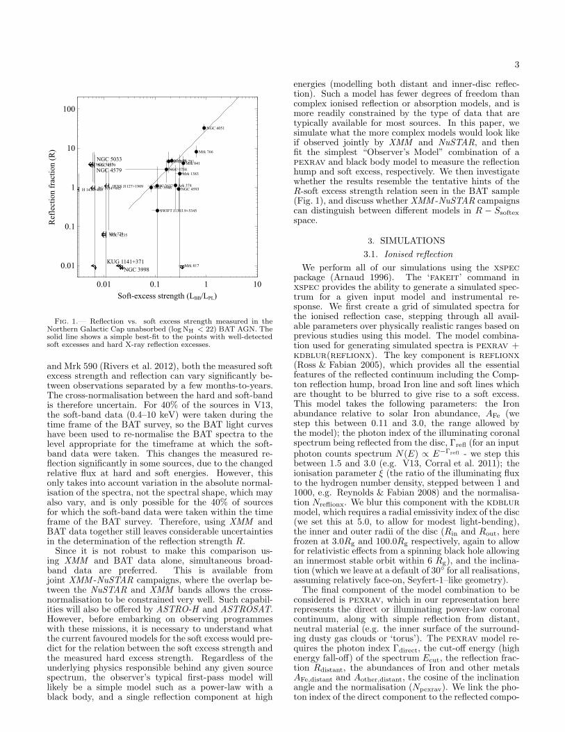
In Vasudevan et al. (2013) (V13 hereafter), we presenta comprehensive analysis of the 100 Northern Galac-tic Cap AGN (b > 50◦) in the 58-month BAT cata-logue. The Swift/BAT instrument provides the mostunbiased census of AGN due to its sensitivity in the14–195 keV band, less prone to the effects of absorp-tion and host-galaxy diluation than any other band, andthe Northern Galactic Cap provides a complete, man-ageable subsample of the catalogue from which to drawstatistically robust conclusions on the AGN population.In V13, BAT and XMM data were used to constrainthe reflection and soft excess strengths in 39 of thesesources, including upper limits where such features werenot detected. The soft excess strength is presented thereas the ratio of the luminosity of the feature (using ablack body to model it) from 0.4–3 keV, to the lumi-nosity in a relatively ‘clean’, feature-free portion of theprimary power-law from 1.5–6 keV. We present belowa plot (Fig. 1) of the reflection strength R against thesoft excess strength Ssoftex = LBB/LPL for those 23 low-absorption sources from V13 (logNH < 22), in whicha soft excess could be detected if present. There arestrong hints of a correlation between R and soft ex-cess strength, but there are also many upper limitingreflection strengths or soft excess strengths which do notsuggest any correlation. This may suggest that differ-ent physical mechanism may account for these two fam-ilies of sources. However, the results using XMM andBAT need to be treated with caution: firstly the BATdata are averaged over many months whereas the XMMdata represent snapshots over a few tens to hundreds ofkiloseconds; they are therefore not simultaneous in anyway, and as is known from NGC 4051 (Ponti et al. 2006)

3

s�(GRRJR5SWR

L(iGSTTF

L(iGJIWT

L(iGI2SS

h��GI2L(iGSWIF

s�(GRRJR5SWRX

R���GxRRXW5RT2T

h��GFRW

-iGX6SW L(iGJITS

L(iGSTTF

��-a�GxRS2SrT5ISJIL(iGJXSI)GRJRT5JF2 L(iGJ2IRh��GW66L(iGIIJF h��GFJRc��GSWJL(iGI2SSh��GWXF/(GRRRJ5JJI h��GRSFSL(iGJIWT

L(iGIXWS

/(GRX2X5XFR

h��GI2

L(iGSWIF

s�(GRRJR5SWRX

R���GxRRXW5RT2T

h��GFRW

-iGX6SWL(iGJITS

L(iGSTTF

��-a�GxRS2SrT5ISJI

L(iGJXSI

)GRJRT5JF2

L(iGJ2IR

h��GW66

L(iGIIJF

h��GFJR

c��GSWJ

L(iGI2SS

h��GWXF

/(GRRRJ5JJI

h��GRSFS

L(iGJIWT

L(iGIXWS

/(GRX2X5XFR h��GI2

L(iGSWIF

s�(GRRJR5SWRX

R���GxRRXW5RT2T

h��GFRW

-iGX6SWL(iGJITS

L(iGSTTF

��-a�GxRS2SrT5ISJI

L(iGJXSI

)GRJRT5JF2

L(iGJ2IR

h��GW66

L(iGIIJF

h��GFJR

c��GSWJ

L(iGI2SS

h��GWXF

/(GRRRJ5JJI

h��GRSFS

L(iGJIWT

L(iGIXWS

/(GRX2X5XFR

�!"#!$%&'(G"�)$%&'(GC�9

2r2R

2rR

R

R2

R22

�'"%M!-$!..G.%�!(/%0GCgttkg/g9

2r2R 2rR R R2

Fig. 1.— Reflection vs. soft excess strength measured in theNorthern Galactic Cap unabsorbed (logNH < 22) BAT AGN. Thesolid line shows a simple best-fit to the points with well-detectedsoft excesses and hard X-ray reflection excesses.

and Mrk 590 (Rivers et al. 2012), both the measured softexcess strength and reflection can vary significantly be-tween observations separated by a few months-to-years.The cross-normalisation between the hard and soft-bandis therefore uncertain. For 40% of the sources in V13,the soft-band data (0.4–10 keV) were taken during thetime frame of the BAT survey, so the BAT light curveshave been used to re-normalise the BAT spectra to thelevel appropriate for the timeframe at which the soft-band data were taken. This changes the measured re-flection significantly in some sources, due to the changedrelative flux at hard and soft energies. However, thisonly takes into account variation in the absolute normal-isation of the spectra, not the spectral shape, which mayalso vary, and is only possible for the 40% of sourcesfor which the soft-band data were taken within the timeframe of the BAT survey. Therefore, using XMM andBAT data together still leaves considerable uncertaintiesin the determination of the reflection strength R.Since it is not robust to make this comparison us-

ing XMM and BAT data alone, simultaneous broad-band data are preferred. This is available fromjoint XMM -NuSTAR campaigns, where the overlap be-tween the NuSTAR and XMM bands allows the cross-normalisation to be constrained very well. Such capabil-ities will also be offered by ASTRO-H and ASTROSAT.However, before embarking on observing programmeswith these missions, it is necessary to understand whatthe current favoured models for the soft excess would pre-dict for the relation between the soft excess strength andthe measured hard excess strength. Regardless of theunderlying physics responsible behind any given sourcespectrum, the observer’s typical first-pass model willlikely be a simple model such as a power-law with ablack body, and a single reflection component at high

energies (modelling both distant and inner-disc reflec-tion). Such a model has fewer degrees of freedom thancomplex ionised reflection or absorption models, and ismore readily constrained by the type of data that aretypically available for most sources. In this paper, wesimulate what the more complex models would look likeif observed jointly by XMM and NuSTAR, and thenfit the simplest “Observer’s Model” combination of apexrav and black body model to measure the reflectionhump and soft excess, respectively. We then investigatewhether the results resemble the tentative hints of theR-soft excess strength relation seen in the BAT sample(Fig. 1), and discuss whether XMM -NuSTAR campaignscan distinguish between different models in R − Ssoftex

space.

3. SIMULATIONS

3.1. Ionised reflection

We perform all of our simulations using the xspecpackage (Arnaud 1996). The ‘fakeit’ command inxspec provides the ability to generate a simulated spec-trum for a given input model and instrumental re-sponse. We first create a grid of simulated spectra forthe ionised reflection case, stepping through all avail-able parameters over physically realistic ranges based onprevious studies using this model. The model combina-tion used for generating simulated spectra is pexrav +kdblur(reflionx). The key component is reflionx(Ross & Fabian 2005), which provides all the essentialfeatures of the reflected continuum including the Comp-ton reflection hump, broad Iron line and soft lines whichare thought to be blurred to give rise to a soft excess.This model takes the following parameters: the Ironabundance relative to solar Iron abundance, AFe (westep this between 0.11 and 3.0, the range allowed bythe model); the photon index of the illuminating coronalspectrum being reflected from the disc, Γrefl (for an inputphoton counts spectrum N(E) ∝ E−Γrefl - we step thisbetween 1.5 and 3.0 (e.g. V13, Corral et al. 2011); theionisation parameter ξ (the ratio of the illuminating fluxto the hydrogen number density, stepped between 1 and1000, e.g. Reynolds & Fabian 2008) and the normalisa-tion Nreflionx. We blur this component with the kdblurmodel, which requires a radial emissivity index of the disc(we set this at 5.0, to allow for modest light-bending),the inner and outer radii of the disc (Rin and Rout, herefrozen at 3.0Rg and 100.0Rg respectively, again to allowfor relativistic effects from a spinning black hole allowingan innermost stable orbit within 6 Rg), and the inclina-tion (which we leave at a default of 30◦ for all realisations,assuming relatively face-on, Seyfert-1–like geometry).The final component of the model combination to be

considered is pexrav, which in our representation hererepresents the direct or illuminating power-law coronalcontinuum, along with simple reflection from distant,neutral material (e.g. the inner surface of the surround-ing dusty gas clouds or ‘torus’). The pexrav model re-quires the photon index Γdirect, the cut-off energy (highenergy fall-off) of the spectrum Ecut, the reflection frac-tion Rdistant, the abundances of Iron and other metalsAFe,distant and Aother,distant, the cosine of the inclinationangle and the normalisation (Npexrav). We link the pho-ton index of the direct component to the reflected compo-

4

nent (Γdirect = Γrefl) and freeze the cut-off energy at themaximal value 106 keV, since current BAT-based studiessuggest that the average cut-off energy for AGN consis-tently lies above a few hundred keV in the majority ofAGN (37 out of 49 AGN fit with pexrav in V13 AGNhave Ecut values consistent with being outside the BATband, or are poorly constrained); at any rate we makethe assumption that it lies outside the NuSTAR band,to consider the simplest case first in our simulations. Wefreeze the abundances at their default values (these rep-resent the abundances of the distant reflector) and keepthe inclination angle at its default value. Nandra et al.(2007) de-convolve distant and inner reflection in a sam-ple of Seyfert AGN, and on average find that the distantcomponent of the reflector has a strengthRdistant = 0.455with a standard deviation σR,dist = 0.295. For each re-alisation of the input spectrum, we randomly generate aGaussian-distributed distant reflection value using theseparameters, to introduce a realistic amount of spread dueto the presence of some distant reflection.Lastly, the crucial parameter in this model set-up is

the ratio of the normalisations of the direct and reflectedcomponents. Before addressing this, we first need tounderstand a complication presented by the publishedversion of the reflionx model: changing the ionisationparameter actually changes the flux of the source in ad-dition to changing the spectrum, so the normalisation isnot a simple flux-multiplier. We modify the table modelsuch that the normalisation is divided out from the ioni-sation parameter, and variations in ξ only produce spec-tral shape changes (not overall flux changes). Havingmade this change, we can use the normalisation of thereflionx model as a simple flux multiplier. We allowthe ratio Npexrav/Nreflionx to go between 1.0 (represent-ing the reflection-dominated case) and 1000.0 (where thepower-law dominates and ionised reflection signaturesshould be barely discernible in the spectrum). We finallyset the overall 1–200 keV flux of the input model to be4 × 10−11erg s−1 cm−2, which is the measured flux forthe well-known Seyfert NGC 4051 using XMM and BATobservations, and the flux of a typical NuSTAR target.Using the above set-up, we now simulate spectra in

both the XMM and NuSTAR bands. We employ more‘pessimistic’ assumptions for the simulated spectra andjust simulate spectra for the PN instrument from XMMand the FPMA instrument from NuSTAR; if more de-tectors are used in data fits, then the accuracy of resultsobtained should only increase. For the simulated XMMspectrum, we use the response and ancillary files froman observation of NGC 4051 reduced in V13, and for theNuSTAR simulated spectrum, we use the latest availablecanned response files for the FPMA instrument. Sinceboth the NuSTAR and XMM responses oversample thespectrum, we re-bin the responses for quicker fits of thesimulated spectra. This was done using the ftools tasksrbnrmf and marfrmf for re-binning the response byuser-specified amounts in each group of channels, and fi-nally combining the effective area file and response file.We again assume a relatively conservative exposure timeof 10 ks in both XMM and NuSTAR, typical of the snap-shots of BAT AGN currently being taken by NuSTAR;longer observations will provide still better constraintson the soft and hard excess strengths. However, the key

1 10 100

10−

30.

01

keV

2 (P

hoto

ns c

m−

2 s−

1 ke

V−

1 )

Energy (keV)

Input model

1 10 100

10−

30.

01

keV

2 (P

hoto

ns c

m−

2 s−

1 ke

V−

1 )

Energy (keV)

Simulated spectrum

Fig. 2.— Model spectrum (top panel) and resultant simulatedNuSTAR and XMM spectra (lower panel), using ionised reflectionas the input model. The simulated spectrum is fit with the simplest“observer’s model” combination pexrav + gauss + bbody. Shortexposure times result in few counts above 50 keV.

point of this study is to see whether physical models forthe soft excess can be distinguished using broad-band X-ray data of typical quality rather than using the longestobservations available, and using simple models ratherthan the more complex, physically motivated models.We present an example of the model spectrum and re-sultant simulated spectrum in Fig. 2.Having simulated the spectra, we group them both us-

ing the grppha tool to have a minimum of 20 countsper bin and re-load the binned spectra into xspec. Weignore any data outside of the range 0.4–10 keV in thesimulated XMM data and any data above 80 keV andbelow 3 keV in the simulated NuSTAR data, as well asignoring any ‘bad’ channels. We then fit the spectra withwhat is henceforth referred to as the “Observer’s model”:the simplest combination of a black body, a gaussian anda pexrav reflection model (bbody + gauss + pexrav)required to account for the components seen in the spec-trum. We use initial conditions that mimic a typicalsoft-excess, power-law, iron-line and hard-excess spectralshape. We set the normalisatoins of the black body, gaus-sian line and pexrav components to be 10−4,10−4 and10−2 respectively, and constrain the black body temper-ature to lie between 0.01 and 2 keV, the line energy to liebetween 6.3 and 7 keV, and the linewidth to lie between0 and 0.5 keV, as is commonly done when fitting real

5

observations. This provides a sensible starting point forthe fit to ensure that the simulated spectra have a goodprobability of being fit successfully.While the soft excess is probably not intrinsically black

body emission and the hump above 10 keV may not in-trinsically be due to reflection, these model componentsserve to parameterise the spectral shape in a way mostcommonly done by observers. The purpose of the firstcomponent is to measure the strength of the soft ex-cess when modelled as a black body, and to calculateits strength using the simple parameterisation LBB/LPL

introduced in V13. The purpose of the gaussian compo-nent is to model the Iron line feature that is naturallyintroduced around 6.4 keV by the reflionx model, andthe purpose of the pexrav component is to measure theoverall strength of the resultant Compton hump, whichwill in general be the sum of both distant and inner re-flection, or an artefact of complex absorption. For dataof typical quality, the abundances and inclination are notusually uniquely determinable so we do not thaw themhere for fitting and freeze them at their defaults. We alsofreeze the cut-off energy at the maximal 106 keV in ourObserver’s model fit, since experience shows that this israrely constrained to be below ∼200 keV in real AGN fitsusing BAT and XMM data (V13). We fit each simulatedspectrum with this Observer’s model, and record all thebest-fit parameters (especially the measured soft excessand reflection strengths) for each set of input (simulated)parameters (AFe, Γdirect, ξ and the ratio of direct-to-reflected components Npexrav/Nreflionx).We step each parameter within the ranges indicated

above, using 7 steps for four primary variables (ξ,Γ,AFe

and Npexrav/Nreflionx), amounting to 2401 total simu-lated spectra. After the fits to the simulated dataare complete, we then plot the ‘measured’ soft excessstrength against the reflection to investigate the presenceof any relation (Fig. 3). We filter out poor fits to the sim-ulated spectra using a dual measurement of the reducedχ2; requiring χ2/d.o.f < 6.0 in the soft band (< 3.0 keV)and χ2/d.o.f < 2.5 in the hard band (> 10 keV), to en-sure that our Observer’s model fits both the soft excessand the hard excess simultaneously; a single band-widereduced χ2 criterion was found to be insufficient to ensurethis. These reduced-χ2 thresholds were chosen by visualinspection of the spectral fits for different cut-off χ2 val-ues, fine-tuning the thresholds until only those spectrawith visually good fits to the soft and hard excesses re-mained. We adopt different reduced-χ2 thresholds in thetwo bands as there are many more bins in the soft bandthan the hard band: it is therefore expected to be moredifficult to get a good fit in the soft band using a sim-ple two-parameter model. A total of 1962 of the 2401fits (82%) were deemed ‘good’ fits according to these cri-teria. The ‘bad’ fits represent parameter combinationsfor which the simple “Observer’s model” could not ad-equately represent the soft and hard excesses. We omiterror bars and do not calculate errors on individual simu-lated spectrum fits, but note that the error on Ssoftex fortypical XMM -quality data are very small, as shown inFig. 1. We know NuSTAR will constrain R much morerobustly than XMM+BAT fits; therefore errors on Rwill assuredly be smaller than in Fig. 1 and errors onSsoftex will be comparable.

�������su���)s �� ����

� �� ����s�

.R.1

.R1

1

1.

1..

���s �� ��s�� ����ls�66���u.Rgcx !)0�#����u1Rhc, !)

.R.1 .R1 1 1.

Fig. 3.— Reflection vs. soft excess strength as measured fromionised reflection simulated spectra. The smaller grey points showall results, and the black points show the results for which theObserver’s model was a ‘good’ fit to the simulated data, using thedual-χ2 criteria given in the text. The contours show the clusteringof the points, with the minimal contours representing 1/13th of thepeak value at the centre of the contours. The gray shaded areashows the expected 1-σ range of reflection strengths from distantreflection from cold material, as found by Nandra et al. (2007).

We see a large degree of spread in Fig. 3, but the con-tours of the highest density of points show a modest butclear trend of increasingR with Ssoftex. Part of the regionof high R (R & 30) shows a high density of points. Per-forming a Kendall’s-τ correlation analysis on the goodfits only yields a correlation coefficient of 0.33 with anull-hypothesis probability < 1× 10−10.

3.2. Ionised absorption

To illustrate the power of the R − Ssoftex diagnosticplot, we also perform this exercise for the ionised windmodel, swind1. Although Schurch & Done (2008) findthis model to require unphysically high terminal veloci-ties of the outflow, a partially-covering ionised absorberwould resolve this problem, and therefore the swind1model can still be taken as representative of an importantclass of multiple-absorber, partially-covering, ionised ab-sorber models that can account for the soft excess. Wetherefore simulate spectra using this model, using therange of parameters identified in the Middleton et al.(2007) study on PG quasars, to see whether such a modelcan produce soft ‘excesses’ and hard ‘excesses’ that canbe modelled as a ‘black body + reflection’ model combi-nation.We use the model combination swind1(pexrav) to

simulate spectra, where the pexrav component repre-sents the primary X-ray continuum along with some dis-tant reflection. In Middleton et al. (2007), a more com-plex model for the primary X-ray power-law and distantreflection is used, but the salient features of such a modelare reproduced here by pexrav for our purposes. We fol-

6

low exactly the same rationale for randomly seeding thedistant reflection with values appropriate for the distri-bution found in Nandra et al. (2007) and follow identicalrationale to that given above in §3.1 for determining theprimary continuum parameters; the primary continuumis common to both the ionised reflection and absorp-tion cases. For the ionised absorption component, westep the column density of the wind between 3 and 50×1022 cm−2; the photon index of the primary continuum(pexrav) Γ between 1.5 and 3; the logarithm of the ion-isation parameter ξ is varied between 2.1 < log(ξ) < 4.0;and the Gaussian velocity dispersion of the wind is var-ied between 0.1 and 0.5, all based on the parametersfound from fitting data on real AGN in Middleton et al.(2007). We simulate spectra in a grid using 7 steps be-tween the maxima and minima for each parameter (seeFig. 4 for example simulated spectra), and plot the re-sulting soft excess strengths and reflection strengths inFig. 5. For this input model, 2073 out of 2401 poten-tial parameter combinations yield successful “Observer’sModel” fits (86%); in the remainder of cases, a ‘blackbody plus reflection’ model combination entirely failedto fit the simulated spectrum (i.e. xspec could not com-pute a fit at all to produce a fit statistic). Using the samedual reduced-χ2 criteria as for ionised reflection, we findthat 1595 of the successful fits were ‘good’ fits (i.e., 77%of successful fits, or 66% of the total 2401 simulated spec-tra).We see a large degree of spread in Fig. 5, without any

clear trend linking R with Ssoftex. Notably, a large num-ber of simulated spectra show prominent soft excesseswith negligible R. Performing a Kendall’s-τ correlationanalysis on the good fits only yields a correlation coeffi-cient of -0.003 with a null-hypothesis probability of 0.88,indicating that there is a high chance of the two proper-ties being completely uncorrelated.

4. DISCUSSION OF RESULTS

At the outset, we note that the “Observer’s Model”produces a successful fit to all of the simulated spec-tra using ionised reflection as the input model, but only86% of the ionised absorption simulated spectra couldbe fit with this model. This indicates that while ionisedabsorption can produce a wide range of spectral shapesthat can mimic the appearance of a soft black body com-ponent with a hard X-ray reflection hump, a substantialminority do not. Sources in those ranges of parameterspace would exhibit spectral shapes clearly distinguish-able from ionised reflection. We discuss this class of spec-tra further in §4.2.The two models compared here show some clearly dis-

tinct behaviour in R− Ssoftex space; the results for bothmodels are plotted in Fig. 6. Notably, in the ionised re-flection scenario, stronger soft excesses can be producedand these are accompanied by stronger measured reflec-tion fractions, particularly for Ssoftex & 1, R & 1. Ionisedreflection as a mechanism for the soft excess could bedistinguishable from distant reflection by a more pro-nounced hard excess (values of R & 2) that one expectsto obtain from such a physical process, coupled with atrend towards higherR at higher Ssoftex, which one wouldexpect to observe in large samples of AGN. This wouldimply that in sources where both 1) strong soft excessesand 2) strong reflection are measured, ionised reflection

1 10 100

10−

30.

01

keV

2 (P

hoto

ns c

m−

2 s−

1 ke

V−

1 )

Energy (keV)

Input model

1 10 100

10−

30.

01

keV

2 (P

hoto

ns c

m−

2 s−

1 ke

V−

1 )

Energy (keV)

Simulated spectrum

Fig. 4.— Model spectrum (top panel) and resultant simulatedNuSTAR and XMM spectra (lower panel), using ionised absorp-tion as the input model. The simulated spectrum is fit with the“observer’s model” combination pexrav + bbody. Short exposuretimes result in few counts above 50 keV.

is the most likely candidate model. For sources with0.5 . R . 3 and Ssoftex . 1, the two models are notimmediately distinguishable.Ionised absorption, on the other hand, can produce

hard excesses with strengths R that are not easily distin-guishable from distant (torus) reflection even if a strongsoft excess is present. This would imply that for sourceswith 1) a strong soft excess (0.3 < Ssoftex < 1) but 2)a not particularly strong hard excess (R . 1), ionisedabsorption may be a candidate model to explain the softexcess, but it could also be due to an altogether differentphysical process, with an unrelated hard excess due todistant, neutral reflection.Chevallier et al. (2006) found that the strongest soft

excesses can be produced by ionised absorption, not re-flection, contrary to our findings here. They investigatedthe different absorber conditions required to reproduceobserved soft excesses in detail, alongside a blurred re-flection model akin to the one we use here but with onekey difference: the reflection spectrum strength is con-strained to be sufficiently lower than that of the primarycontinuum such that prominent soft excesses cannot beseen. In our model, the ratio of the direct pexravcontinuum to the reflionx continuum is widely vari-able to account for light-bending effects (e.g., the coro-nal height varying above the accretion disc), and when

7

�������su���)s �� ����

� �� ����s�

.R.1

.R1

1

1.

1..

���s �� ��s�� ����ls�66���u.Rgcx !)0�#����u1Rhc, !)

.R.1 .R1 1 1.

Fig. 5.— Reflection vs. soft excess strength as measured fromionised absorption simulated spectra. Key as for Fig. 3

Npexrav/Nreflionx ∼ 1, strong soft excesses can be ob-served, as seen in reflection-dominated epochs of sourcessuch as NGC 4051 (Ponti et al. 2006). Full considerationof the effects of light-bending at the inner parts of theaccretion flow allows the reflection spectrum to dominateand produce such strong excesses.Some very interesting behaviour is seen at the extrema

of Fig. 6. Both ionised reflection and absorption allowfor non-detected soft excesses alongside moderate reflec-tion (0.2 < R < 3.0), but ionised absorption allows fora large range of soft excess strengths alongside negligi-ble or no measured hard excess. Therefore, in sourceswhere the soft excess is prominent but reflection is un-detectable, it may be appropriate to consider partially-covering ionised absorption or other non-reflection basedmodels (e.g., Comptonisation). Finally, the region of theplot showing strong soft excesses Ssoftex > 1 and rela-tively weak hard excesses R < 1 is not populated byeither of the two models considered here. Further workneeds to be done to explore if other models can occupythis part of parameter space.We can apply these diagnostics now to the objects

in Fig. 1, although with the caveat that those resultswere obtained using non-simultaneous hard- and soft-X-ray data, without the overlap between the soft andhard band required to constrain reflection well. Nev-ertheless, one can suggest (subject to further investi-gation with better data) that those objects in whichreflection and soft excess strength seem to be increas-ing together likely have a strong contribution fromionised reflection. NGC 4051 has been studied in depthand it is known that ionised reflection can be fit tothe detailed 0.4–10 keV spectrum (Ponti et al. 2006,Alston et al. 2013). Reflection has been suggested forMrk 766 also (Emmanoulopoulos et al. 2011); but com-plex, multi-layered absorbers (perhaps a disk wind), and

�������su���)s �� ����

� �� ����s�

.R.1

.R1

1

1.

1..

���s �� ��s�� ����s���� �sks�66lu.Rgcx !0�#�l1Rhc= !

.R.1 .R1 1 1.

Fig. 6.— Contours of reflection vs. soft excess strength from bothionised reflection and ionised absorption models, for comparison.

occultation by absorbing clouds have also been invoked(Turner et al. 2007; Risaliti et al. 2011). Both ionised re-flection and absorption can explain the spectrum of Mrk841 (Cerruti et al. 2011). The object Mrk 817, which hasnegligible reflection but a measurable soft excess, maywell require a different model such as ionised absorptionto account for its soft features. Indeed, Winter et al.(2011) mention an epoch in this source where absorbingwinds were detected in UV spectroscopy of this sourcefrom 1997 and 2009, albeit without the X-ray edges dueto Oxygen expected at 0.73 and 0.87 keV from suchoutflows. One potential explanation may be that the> 2 keV X-ray continuum in this source is absorbed bya highly relativistic ionised absorber, which may tallywith the absorption signatures in the UV. Again, datathat extends into the > 10 keV band would provide moredefinitive answers, stressing the utility of the approachoutlined in this paper.Two Narrow-Line Seyfert 1 nuclei with strong soft ex-

cesses have recently been studied in detail using XMMdata: 1H 0707-495 and IRAS 13224-3809. Fabian et al.(2012) and Dauser et al. (2012) find that reflection cansuccessfully fit the spectrum of 1H 0707-495; Kara et al.(2013) and Fabian et al. (2013) find the same for IRAS13224-3809. We use the archival XMM data to estimateSsoftex for both of these sources and find that they are3.3 (1H 0707-495) and 2.6 (IRAS 13224-3809); thereforeaccording to the scheme found in this paper, their softexcesses are both sufficiently strong to favour a reflection-dominated scenario. Broad-band observations with NuS-TAR should be able to confirm this and locate both ob-jects on the R− Ssoftex plot.

4.1. Extreme values of the hard excess strength,R & 100

8

For both models tested in this paper, there are acluster of points at R & 100, which have not so farbeen observed in the real AGN population. For theionised reflection case, further investigation reveals thatall of the simulated spectra that produce R > 100 haveNpexrav/Nreflionx < 10, and all of the very extreme Rvalues (i.e. R > 200) measured from ‘good’ fits haveNpexrav/Nreflionx = 1, the lowest value of the ratio in-cluded in the simulations, corresponding to the mostreflection-dominated case (see Fig. 7, top panel). Thissuggests that for reflection-dominated spectra, the spec-tral shapes produced can genuinely give rise to veryhigh, ‘anomalous’ R values (under the fitting assump-tions adopted in this study), depending on the spreadof other intrinsic parameters i.e. AFe, ξ and Γ. Wethen focus only on the subset of objects with reflection-dominated spectra (1 < Npexrav/Nreflionx < 10, Fig. 7,lower panel). We split the results into different bins ofAFe, ξ and Γ, selecting 3 bins for each (using logarithmicspacing for ξ). We find that the ionisation parameterξ produces the greatest variation in measured R. Thelowest ionisation parameters, 1.0 < ξ < 10.0, give rise toalmost all of the R > 100 points. In conclusion, the mostreflection-dominated spectra (1.0 < Npexrav/Nreflionx <10.0) coupled with the most weakly ionised reflectors(1.0 < ξ < 10.0) can produce very strong hard excesses.This range of R values has not been seen in the real

AGN population so far, but only a handful of obser-vations currently exist of reflection-dominated states ofAGN (e.g., Zoghbi et al. 2008; Fabian et al. 2012). Suchprominent hard excesses may be found with new NuS-TAR observations. Since the ionisation parameter isproportional to the luminosity, the very low luminositysources (with potential for the most prominent hard ex-cesses) may also be selected out of most X-ray surveys.For the ionised absorption model, the highest values of

the measured R occur for log(ξ) < 2.75. From inspectionof the spectra, we find that many of these low ionisationabsorbers have absorption troughs that look more likeextended ‘edges’. The hard portion of the spectrum canthen be fit as a pure reflection component in some cases,leading to high values of R. In the remainder of low-ionisation absorber spectra, the slope of the intermediate(3—10 keV) region is too extreme to be fit by the pexravcomponent and the fit fails altogether (discussed furtherin §4.2).We also consider the possibility that the low exposure

time (10ks) and resulting poor-quality data at high en-ergies could lead to such anomalous R values. However,increasing the observation time to 20ks (for both ionisedreflection and absorption models, Fig. 8) did not produceany significant change in the results and the broad trendsseen.

4.2. Failed fits with ionised absorption

As mentioned in §3.2, 14% of the simulated ionised ab-sorption spectra result cannot be fit with the Observer’sModel. We investigate this class of objects in more de-tail. We find that the only weak discriminant of whethera spectrum fits successfully or not is the ionisation pa-rameter of the absorber, log(ξ). Failed fits only occur forspectra simulated with 2.1 < log(ξ) < 2.75. There are1029 possible parameter combinations/simulated spec-tra in this range (i.e., 3 bins in log(ξ) and 7 bins for

Fig. 7.— Measured hard excess and soft excess strength for theionised reflection scenario, split by 1) ratio of direct-to-reflectedcomponent Npexrav/Nreflionx (top panel), and 2) ionisation param-eter ξ (lower panel). In the top panel, small and large black cir-cles represent simulated spectra with 1 < Npexrav/Nreflionx < 10(successful fits and ’good’ fits respectively); red crosses (suc-cessful fits) and red circled crosses (good fits) represent 10 <Npexrav/Nreflionx < 100 spectra, and green X symbols (success-ful fits) and green X symbols within squares (good fits) represent100 < Npexrav/Nreflionx < 1000 spectra. In the lower panel,the same sequence of symbol combinations is used to split thereflection-dominated (1 < Npexrav/Nreflionx < 10) subset of spec-tra into groups with 1 < ξ < 10, 10 < ξ < 100 and 100 < ξ < 1000,respectively. The colours of the upper/lower limit arrows matchesthe colours of the points for the corresponding parameter groups,and the size of the upper/lower limit symbols increases going fromsmall-to-high values of Npexrav/Nreflionx and ξ.

each other parameter), out of which 328 model combi-nations fail completely. On inspection, these spectra ex-hibit ionised absorber troughs that look more like edgeswith a very steep rise in flux towards higher energies.When manually fit with the observer’s model combina-

9

Fig. 8.— Simulation results for the R − S diagram with an ob-servation time of 20 ks. Key as for Fig. 3.

tion, we find that the fits consistently fail. The power-lawregime of the pexrav component attempts to fit to therising part of the edge below 10 keV, but the photon in-dex required is too extreme (see Fig. 9). This would be areadily identifiable subset of spectral shapes which can-not be fit with a simple black body and reflection model,and any soft ‘excess’ seen would clearly be distinguish-able from one produced by ionised reflection.Of the remaining 701 low-log ξ spectra which are suc-

cessfully fit by the Observer’s model, only 50% qualify as’good fits’ according to the dual-χ2 criteria. Inspection ofthese ‘good fits’ reveals that the power-law component isable to fit the rising 1–6 keV portion of the spectrum suc-cessfully. It is therefore not straightforward to identifya very specific part of ionised-absorber parameter spacethat eludes fitting with the Observer’s model, but we cansay that the failing of the fit is restricted to low-ionisationabsorbers. The success rate of fitting such unusual spec-tral shapes may also be subtly dependent on the initialconditions employed in the Observer’s model, the explo-ration of which is beyond the scope of this paper.

4.3. Predictions for other comparable instruments

We have presented results for the XMM-NuSTAR in-strument combination since NuSTAR is newly launchedand this instrument combination is already being usedto obtain simultaneous broad-band X-ray data on AGN(e.g., Risaliti et al. 2013; Matt et al. 2014); therefore itis the most relevant prediction for the current circum-stances with real near-term prospects of verifying thework in this paper. ASTRO-H and ASTROSAT are alsoon the horizon, and to check whether our predictions holdfor other instruments, we also perform simulations forthe ionised reflection model using the current ASTRO-H predicted response matrices, assuming the same 10 ksexposure time. We caution that these responses may be

1 10

10−

30.

015×

10−

42×

10−

35×

10−

3

keV

2 (P

hoto

ns c

m−

2 s−

1 ke

V−

1 )

Energy (keV)

Ionised absorption: successful fit to low−ionisation absorber

1 1010−

410

−3

0.01

keV

2 (P

hoto

ns c

m−

2 s−

1 ke

V−

1 )

Energy (keV)

Ionised absorption: failed fit

Fig. 9.— Example spectra with low-ionisation ionised ab-sorbers, showing the attempted Observer’s Model fit using thepexrav+bbody model combination. Top panel : example of a suc-cessful fit. The input parameters for the simulated spectrum areΓ = 2.0, NH = 5.0 × 1023cm−2, log ξ = 2.73, σ = 0.43. Lowerpanel : example of a failed fit. The input parameters are Γ = 2.0,NH = 1.87 × 1023cm−2, log ξ = 2.42, σ = 0.23.

more uncertain than the XMM+NuSTAR responses, asreal responses are likely to differ significantly from thepre-launch predicted ones. The resulting R− S diagramdoes not show any significant difference to that obtainedfor XMM-NuSTAR (Fig. 10), suggesting that the con-clusions in this paper should hold for other similarly-equipped future broad-band X-ray observatories.

4.4. On the feasibility of observing these trends in realAGN samples

The simulations here outline the trends expected inR − Ssoftex space for two different models using a largegrid of 2401 parameter combinations. AGN samples aretypically much smaller due to the competition for obser-vation time, so we require a measure of how feasible itwill be to detect these trends in real samples of AGN.We perform further simulations to estimate the typicalAGN sample size required, before a correlation (or theabsence of one) can be seen between R and Ssoftex.We use a Monte-Carlo rejection method to simulate

N values of R and Ssoftex (corresponding to a sample ofN AGN) randomly determined throughout the availableR − Ssoftex space, using the contours determined fromFigs. 3 and 5 as the probability distribution with whichto distribute the points in R− Ssoftex space. We vary Nand measure the resultant Kendall’s τ correlation coeffi-cient of the faked sample to determine when the strengthof the correlation approaches that seen in the full simula-tions. We do this for both ionised reflection and ionisedabsorption. The variation of the correlation coefficient

10

Distant (torus) reflection

Reflection R

0.01

0.1

1

10

100

Soft excess strength, LBBonly(0.4-3keV)/LPLonly(1.5-6keV)

0.01 0.1 1 10

Fig. 10.— Results for ionised reflection using the ASTRO-H re-sponse matrices. Key as for Fig. 3.

�������n���� ���

�������n������ ���

������c�n����������

�τK0

�τK−

τ

τK−

τK0

τK.

τK2

τK1

�����n����n�

τ 0τ 2τ 3τ 5τ −ττ

Fig. 11.— Kendall’s τ correlation coefficient between R andSsoftex against sample size, for a simulated AGN sample of sizeN . The solid (black) and dashed (red) lines show the correlationcoefficients measured for the whole set of simulations (correspond-ing to N > 1500), for ionised reflection and ionised absorptionrespectively. The error bar shows the standard deviation from100 Monte-Carlo realisations of such samples of N objects, andindicates that as N approaches ∼ 60, the correlations exhibitedby samples of predominantly reflection-dominated or absorption-dominated samples can be clearly distinguished.

with N for each input model is shown in Fig. 11.We see that at N & 60, the uncertainty in the corre-

lation coefficients produced by the two processes dropssuch that the two processes can be distinguished at a2–3σ level. Therefore, even though the physical processmay be ambigious for an individual object based on itslocation in the R − Ssoftex plane, the trend exhibited bya well-selected, representative AGN sample in this planecan provide an indication of the physics most relevantfor the majority of AGN in the sample.

4.5. Outstanding issues

We outline some issues to be further explored in futurework. Firstly, the ratioNpexrav/Nreflionx is currently usedas an estimator of the degree of light bending in the re-flection scenario. A more physical understanding of thisparameter is needed to place appropriate upper and lowerlimits on it for the simulations. It is easy to conceive of asituation where the direct power-law dominates; howeverunderstanding the lower-limit on the range of physicallyviable ratios (here assumed to be Unity) is more complexand requires a fuller consideration of the energetics of thereflection-dominated state than is undertaken here. Thismay impact the strongest observable strengths of the softexcess from the reflection scenario, as initially investi-gated by Chevallier et al. (2006), but the observation ofAGN in fully reflection-dominated states does supportthe possibility that Npexrav/Nreflionx can take very lowvalues (even < 1).We have assumed uniform or log-uniform distributions

for the input parameters in these simulations, as the sim-plest possible scenario. However, it may be the casethat the real underlying distributions are not uniform, orthat there are correlations between the input parameters.There are a handful of studies on this in the literature,presenting the photon index and luminosity distribu-tions in AGN (e.g., Corral et al. 2011, Vasudevan et al.2013). Previous works (e.g.,Reynolds & Fabian 2008;Ballantyne et al. 2011) have found a range of ionisationparameters for ionised reflection consistent with that as-sumed here. There are suggestions of a weak correlationbetween photon index and luminosity (e.g., Saez et al.2008) hence potential for a correlation between Γ and ξ.However, there is no detailed work on the true underly-ing distributions of physical parameters of reflectors. It ispossible that the observed trends highlighted in this workin the R− S plane could be changed, and the density ofpoints in different parts of the plot could be altered, ifdifferent underlying distributions are used. To allow forthis to be investigated in future, we make our simulationresults public with the online data accompanying thispaper. The interested researcher can then draw from theprovided results in a non-uniform way using more up-dated distributions or correlations between parameters,as and when such details become more well-constrained.However, one instinctively expects some degree of cor-relation between hard- and soft-excess strengths in theionised reflection scenario, regardless of the precise un-derlying parameter distributions.One of the latest models to be proposed for the soft

excess is the optxagnf model (Done et al. 2012). Theirmodel combines disk emission, Comptonisation and apower-law in an energetically self-consistent way, wherethe inner part of the accretion flow below a coronal ra-dius is Comptonised to produce the soft excess. Comp-tonisation is the engine behind the soft excess in this

11

model, and one does not expect it to exert any influenceon the hard X-ray emission based on simple models (e.g.,Page et al. 2004) providing a purely standalone compo-nent for the soft excess. Therefore, one does not expectany link between the soft excess and hard excess in thisscenario. However, this may not be the case for optx-agnf where the disc and corona geometries are linkedby energetic considerations, and we are currently under-taking a study of this model in detail, with a view toproduce a similar R− Ssoftex diagnostic plot to compareit with the models in this paper. The optxagnf modelis able to fully reproduce the optical–to–X-ray SED up to10 keV, as shown by the comprehensive study of Jin et al.(2012), but its hard X-ray signatures have not been stud-ied. Additionally, distant reflection needs to be added ina consistent fashion if we want to compare it with themodels studied here, where pexrav was used to providethe direct continuum along with the distant reflection.How to do this is not clear, and since optxagnf hasmany more model parameters to consider than the mod-els in this paper, we defer this study to a future paper(in prep.).

5. SUMMARY

This work points to a scheme whereby different candi-date models for the soft excess can be distinguished in aplot of measured reflection against soft-excess strength,assuming the simplest possible pexrav + bbody modelcombination is fit to the spectra, according to the schemein Fig. 6. This methodology can readily be extended toother candidate models, and we are currently in the pro-cess of producing such a diagnostic for the optxagnfmodel, where photons from the inner part of the ac-cretion disc are Comptonised to produce the soft excess(Done et al. 2012). A key advantage of this approach isits economy: data of moderate quality can be used, gath-ered using short exposures (e.g. 10 ks in both XMM andNuSTAR for a source of the brightness of NGC 4051)to gain real physical insight into the energy productionmechanisms in AGN, without requiring fitting of morecomplex models to long-exposure, very high signal-to-

noise ratio data. This approach will therefore be usefulin constraining the soft excess mechanism in samples ofAGN, where it may be challenging to obtain such longexposures on each source. This approach is particularlyuseful for samples of AGN where trends can be discerned,although it can be used for individual AGN as well, ifthey lie in unambigious regions of R− Ssoftex space. No-tably, ionised reflection predicts a clear relation betweenR and Ssoftex, but ionised absorption does not.As simultaneous or broad-band X-ray data comes in

from NuSTAR+XMM, ASTRO-H and ASTROSAT, thisplot can be populated with accurate, simultaneous deter-minations of the strengths of the hard and soft excessesin samples of real AGN, updating the work presented inFig. 1. Using the contours presented in Fig. 6 as proba-bility contours, we simulate a smaller sample of AGN us-ing a Monte-Carlo Rejection method, and estimate that∼ 60 AGN would be sufficient to verify the existence of aR − Ssoftex correlation of comparable strengths to thosefound in our original simulations (Figs 3 and 5). Thiswould amount to an easily achievable XMM -NuSTARcampaign of ∼600 ks.It will be easier to narrow down the mechanism respon-

sible for producing the soft excess in any given source, ifit is first fit with the simplest possible “observer’s model”outlined here to locate it on the R − Ssoftex plot. Addi-tionally, the regions of this plot occupied by large samplesof AGN will also provide an indication of the most likelysoft excess production mechanisms in the AGN popula-tion as a whole. The general simulation methodologyadopted here also has much potential for distinguishingbetween competing models in other areas of both AGNscience and other fields of astrophysics.

6. ACKNOWLEDGEMENTS

We thank the anonymous referee for useful sugges-tions which improved the paper. CSR thanks NASA forsupport under grant NNX12AE13G. We thank JeremySanders for help with the use of his Veusz plotting pack-age, and Cole Miller for helpful discussions on Monte-Carlo simulation techniques.

REFERENCES

Alston, W. N., Vaughan, S., & Uttley, P. 2013, MNRAS, 435,1511

Arnaud, K. A. 1996, in Astronomical Society of the PacificConference Series, Vol. 101, Astronomical Data AnalysisSoftware and Systems V, ed. G. H. Jacoby & J. Barnes, 17

Arnaud, K. A., Branduardi-Raymont, G., Culhane, J. L., et al.1985, MNRAS, 217, 105

Ballantyne, D. R., McDuffie, J. R., & Rusin, J. S. 2011, ApJ, 734,112

Cerruti, M., Ponti, G., Boisson, C., et al. 2011, A&A, 535, A113Chevallier, L., Collin, S., Dumont, A.-M., et al. 2006, A&A, 449,

493Corral, A., Della Ceca, R., Caccianiga, A., et al. 2011, A&A, 530,

A42Crummy, J., Fabian, A. C., Gallo, L., & Ross, R. R. 2006,

MNRAS, 365, 1067D’Ammando, F., Bianchi, S., Jimenez-Bailon, E., & Matt, G.

2008, A&A, 482, 499Dauser, T., Svoboda, J., Schartel, N., et al. 2012, MNRAS, 422,

1914De Marco, B., Ponti, G., Cappi, M., et al. 2013, MNRAS, 431,

2441Done, C., Davis, S. W., Jin, C., Blaes, O., & Ward, M. 2012,

MNRAS, 420, 1848Emmanoulopoulos, D., McHardy, I. M., & Papadakis, I. E. 2011,

MNRAS, 416, L94

Fabian, A. C., Zoghbi, A., Ross, R. R., et al. 2009, Nature, 459,540

Fabian, A. C., Zoghbi, A., Wilkins, D., et al. 2012, MNRAS, 419,116

Fabian, A. C., Kara, E., Walton, D. J., et al. 2013, MNRAS, 429,2917

Gierlinski, M., & Done, C. 2004, MNRAS, 349, L7Harrison, F. A., Craig, W. W., Christensen, F. E., et al. 2013,

ApJ, 770, 103Holt, S. S., Mushotzky, R. F., Boldt, E. A., et al. 1980, ApJ, 241,

L13Jin, C., Ward, M., Done, C., & Gelbord, J. 2012, MNRAS, 420,

1825Kara, E., Fabian, A. C., Cackett, E. M., Miniutti, G., & Uttley,

P. 2013, MNRAS, 430, 1408Laha, S., Dewangan, G. C., Chakravorty, S., & Kembhavi, A. K.

2013, ApJ, 777, 2Magdziarz, P., & Zdziarski, A. A. 1995, MNRAS, 273, 837Matt, G., Marinucci, A., Guainazzi, M., et al. 2014, ArXiv

e-printsMiddleton, M., Done, C., & Gierlinski, M. 2007, MNRAS, 381,

1426Miller, L., & Turner, T. J. 2013, ApJ, 773, L5Miniutti, G., Ponti, G., Greene, J. E., et al. 2009, MNRAS, 394,

443Nandra, K., O’Neill, P. M., George, I. M., & Reeves, J. N. 2007,

MNRAS, 382, 194

12

Page, K. L., Schartel, N., Turner, M. J. L., & O’Brien, P. T.2004, MNRAS, 352, 523

Paul, B. 2013, International Journal of Modern Physics D, 22,41009

Ponti, G., Miniutti, G., Cappi, M., et al. 2006, MNRAS, 368, 903Ponti, G., Gallo, L. C., Fabian, A. C., et al. 2010, MNRAS, 406,

2591Pravdo, S. H., Nugent, J. J., Nousek, J. A., et al. 1981, ApJ, 251,

501Reynolds, C. S., & Fabian, A. C. 2008, ApJ, 675, 1048Risaliti, G., Nardini, E., Salvati, M., et al. 2011, MNRAS, 410,

1027Risaliti, G., Harrison, F. A., Madsen, K. K., et al. 2013, Nature,

494, 449Rivers, E., Markowitz, A., Duro, R., & Rothschild, R. 2012, ApJ,

759, 63Rivers, E., Markowitz, A., & Rothschild, R. 2013, ApJ, 772, 114Ross, R. R., & Fabian, A. C. 2005, MNRAS, 358, 211Saez, C., Chartas, G., Brandt, W. N., et al. 2008, AJ, 135, 1505Schurch, N. J., & Done, C. 2008, MNRAS, 386, L1Singh, K. P., Garmire, G. P., & Nousek, J. 1985, ApJ, 297, 633Takahashi, T., Mitsuda, K., Kelley, R., et al. 2012, in Society of

Photo-Optical Instrumentation Engineers (SPIE) ConferenceSeries, Vol. 8443, Society of Photo-Optical InstrumentationEngineers (SPIE) Conference Series

Tatum, M. M., Turner, T. J., Miller, L., & Reeves, J. N. 2013,ApJ, 762, 80

Turner, T. J., Miller, L., Kraemer, S. B., Reeves, J. N., &Pounds, K. A. 2009, ApJ, 698, 99

Turner, T. J., Miller, L., Reeves, J. N., & Kraemer, S. B. 2007,A&A, 475, 121

Vasudevan, R. V., Brandt, W. N., Mushotzky, R. F., et al. 2013,ApJ, 763, 111

Walton, D. J., Nardini, E., Fabian, A. C., Gallo, L. C., & Reis,R. C. 2013, MNRAS, 428, 2901

Walton, D. J., Reis, R. C., & Fabian, A. C. 2010, MNRAS, 408,601

Winter, L. M., Danforth, C., Vasudevan, R., et al. 2011, ApJ,728, 28

Zhong, X., & Wang, J. 2013, ApJ, 773, 23Zoghbi, A., Fabian, A. C., & Gallo, L. C. 2008, MNRAS, 391,

2003Zoghbi, A., Fabian, A. C., Uttley, P., et al. 2010, MNRAS, 401,

2419