draft report dispersion modeling of drilling applied

Applied Science Associates A member of the RPS Group plc

55 Village Square Drive South Kingstown, RI 02879 USA Tel: +1 (401) 789-6224 Fax: +1 (401) 789-1932 www: www.rpsgroup.com www: www.asascience.com

Draft Report

Dispersion Modeling of Drilling Discharges: Deepwater Tano Block,

offshore Ghana

AUTHOR(S): Nathan Vinhateiro, Tatsu Isaji, Eric Comerma

Project Manager: Nathan Vinhateiro

PROJECT NUMBER:

ASA 13-176

VERSION: Rev1

DATE: 29 Jan 2014

CLIENT:

John Ward, Mark Irvine Environmental Resources Management, London, UK

http://www.rpsgroup.com/

http://www.asascience.com/

ERM | Ghana (TGL) 13-176, 29 January 2014

Applied Science Associates

a member of the RPS Group plc i

Document Control Form

Title:

“Dispersion Modeling of Drilling Discharges: Deepwater Tano Block, offshore Ghana.”

Location & Operator:

Enyenra Field, Deepwater Tano License Block. Tullow Ghana Limited (TGL).

ASA Project Number: 13-176 ERM Ghana Drilling

Author List: Nathan Vinhateiro, PhD, Oceanographer

Tatsu Isaji, Senior Scientist

Eric Comerma, PhD, Ocean Engineer, Senior Scientist

Project Manager: Nathan Vinhateiro, PhD, Oceanographer

Release File Name Date Submitted Notes

Preliminary 13-176_ERM_Ghana_Prelim_20Dec2013 20 December 2013 Preliminary model results

Draft 13-176_ERM_Ghana_Draft_17Jan2014 17 January 2014 Complete modeling report (draft)

Draft (Rev1) 13-176_ERM_Ghana_Draft_29Jan2014 29 January 2014 Revised to include ERM comments

Disclaimer:

This document may contain confidential information that is intended only for use by the client and is not for public circulation, publication, or third party use without consent of the client. The client understands that modeling is predictive in nature and while this report is based on information from sources that Applied Science Associates, Inc. considers reliable, the accuracy and completeness of said information cannot be guaranteed. Therefore, Applied Science Associates, Inc., its directors, agents, assigns, and employees accept no liability for the result of any action taken or not taken on the basis of the information given in this report, nor for any negligent misstatements, errors, and omissions. This report was compiled with consideration for the specified client's objectives, situation, and needs.



a member of the RPS Group plc ii

Executive Summary Environmental Resources Management (ERM) contracted with Applied Science Associates, Inc. (dba RPS-ASA) to evaluate seabed deposition and suspended sediment concentrations associated with operational discharges within the Deepwater Tano (DWT) license block, offshore Ghana. Two drilling sites within the Enyenra field (En07-WI and En13-WI) were selected for the dispersion modeling to represent different water depths along the continental slope. The sites are located approximately 50-70 km south of the coast at water depths of 1330 m and 1990 m, respectively. The study consisted of simulating the release of drill cuttings and drilling mud at each site for up to four drilling sections, using varying current conditions over a period of 15 consecutive days. Simulations were performed to evaluate seabed deposition and sediment plumes following the discharge of cuttings treated with a thermal desorption unit (TDU). Discharge simulations were completed using ASA’s MUDMAP modeling system. The MUDMAP model predicts the transport of solid releases in the marine environment and the resulting seabed deposition. The model requires information regarding the discharge characteristics (release location, rate of discharge, etc.), the properties of the sediment (particle sizes, density), and environmental characteristics (bathymetry and ocean currents), to predict the transport of solids through the water column. The general ocean circulation in the DWT block is strongly influenced by the behaviour of the Guinea Current. Modeling and observational studies have noted that this feature exhibits minimum velocities during the autumn months and maximum during the spring/summer. Because drilling in the DWT block is expected to occur throughout the year, MUDMAP simulations were performed for different periods to examine the potential effect of seasonal circulation patterns. Releases were simulated during the months of April and December – which correspond to periods used during previous modeling for the TEN Development (ASA project 11-053). Peak, eastwardly oriented surface currents characterize the flow regime during April, whereas currents during December are less intense and more directionally variable. For each scenario, vertically and time varied currents derived from the HYCOM (HYbrid Coordinate Ocean Model) global simulation were used to reproduce the density and wind-driven circulation in the tropical Atlantic. Currents used as model inputs were obtained at a daily resolution. The resulting bottom deposition from individual discharge sections was analysed along with the pattern of cumulative deposits for each site and season. All scenarios predict a generally rounded and tight depositional footprint that surrounds each well head. Contours representing very fine thickness intervals (0.1 mm) are slightly more elongate and extend up to 620 m from the release site. The areal extent of deposition above 1 mm is nearly indistinguishable between sites/seasons. The similarities are primarily due to the occurrence of very weak bottom currents at both sites, and the treatment of cuttings returned to the surface. The TDU process results in extremely fine particles that do not contribute significantly to the cumulative mass accumulation on the seabed. Considering all scenarios, thicknesses at or above 1 mm are confined to a distance of 96 m from the discharge sites and occupy a maximum areal extent of 0.02195 km2; thicknesses greater than 10 mm extend up to 48 m with a maximum footprint of 0.00599 km2. MUDMAP was also used to assess total suspended solid (TSS) concentrations associated with the drilling operation for representative current regimes. A total of eight MUDMAP scenarios (2 sites x 2 seasons x 2 flow regimes) were performed to simulate the water column plume associated with discharge of TDU



a member of the RPS Group plc iii

powder from the Mobile Offshore Drilling Unit (MODU). As with seabed deposition, the excess TSS near the water surface is highly dependent on the hydrodynamic forcing on the day of the cuttings release. Sediment plumes resulting from discharges of TDU powder are predicted to extend between 230 and 360 m from the MODU. In general, the extent of the plumes is greater during strong current conditions, while the maximum TSS concentrations increase during weak current conditions and the plumes persist for longer periods. The maximum predicted concentration of suspended sediments in the water column (corresponding to the weakest current regime) is 896 mg/L. In all cases, the water column is predicted to return to ambient conditions (<10 mg/L) within an hour of the final release.



a member of the RPS Group plc iv

Table of Contents Executive Summary ....................................................................................................................................... ii

1. Introduction .............................................................................................................................................. 7

2. Geographic Location and Environmental Data ......................................................................................... 8

2.1. Study Location .................................................................................................................................... 8

2.2. Regional Circulation and Current Datasets ........................................................................................ 9

3. Drilling Discharge Simulations................................................................................................................. 20

3.1. Model Description - MUDMAP ........................................................................................................ 20

3.2. Discharge Scenarios ......................................................................................................................... 20

3.3. Discharge sediment characteristics ................................................................................................. 21

4. Results of the Drilling Discharge Simulations ......................................................................................... 25

4.1. Predicted deposition thickness ........................................................................................................ 25

4.2. Predicted Water Column Concentrations ........................................................................................ 31

5. Conclusions ............................................................................................................................................. 37

6. References .............................................................................................................................................. 38

Appendix A: MUDMAP Model Description ................................................................................................. 40



a member of the RPS Group plc v

List of Figures Figure 1. Map of the proposed discharge sites: En13-WI, and En07-WI. Dashed line shows the maritime boundary

between Ghana (East) and Côte d’Ivoire (West). ................................................................................... 8 Figure 2. General circulation in the Gulf of Guinea region (Hardman-Mountford and McGlade, 2003). Solid arrows

represent surface currents and hatched arrows represent undercurrents: EUC=Equatorial Undercurrent, GC=Guinea Current, GUC=Guinea Undercurrent, NECC=North Equatorial Counter Current. ................................................................................................................................................... 9

Figure 3. Seasonal trends of the Guinea Current (Source: Gyory et al., 2005). Vectors indicate the average current directionality for each period and the white outlined vectors mark the extent of the Guinea Current. .............................................................................................................................................................. 10

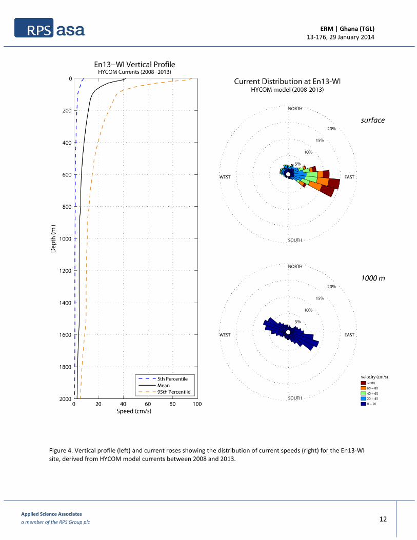
Figure 4. Vertical profile (left) and current roses showing the distribution of current speeds (right) for the En13-WI site, derived from HYCOM model currents between 2008 and 2013. ................................................. 12

Figure 5. Vertical profile (left) and current roses showing the distribution of current speeds (right) for the En07-WI site, derived from HYCOM model currents between 2008 and 2013. ................................................. 13

Figure 6. Monthly averaged current speeds at En13-WI derived from the HYCOM global dataset. Average current speeds are shown for the surface (top) and 1000 m (bottom) water depths. ..................................... 14

Figure 7. Monthly averaged current speeds at En07-WI derived from the HYCOM global dataset. Average current speeds are shown for the surface (top) and 1000 m (bottom) water depths. ..................................... 15

Figure 8. Current roses showing the distribution of surface currents (speed and direction) by month at the En13-WI site, derived from HYCOM model currents between 2008 and 2013. ................................................. 16

Figure 9. Current roses showing the distribution of surface currents (speed and direction) by month at the En07-WI site, derived from HYCOM model currents between 2008 and 2013. ................................................. 17

Figure 10. Time series of HYCOM model currents with depth at the En13-WI discharge site. Shading indicates the simulation periods (Apr 1-16 and Dec 1-16, 2012). .............................................................................. 18

Figure 11. Time series of HYCOM model currents with depth at the En07-WI discharge site. Shading indicates the simulation periods (Apr 1-16 and Dec 1-16, 2012). .............................................................................. 19

Figure 12. Comparison of settling velocities for solid discharges used in the modeling study. Size class divisions are from Gibbs et al. (1971). ....................................................................................................................... 24

Figure 13. Cumulative deposition thickness (cuttings and mud) at En13-WI using April 2012 (top) and December 2012 (bottom) current conditions. ....................................................................................................... 27

Figure 14. Cumulative deposition thickness (cuttings and mud) at En07-WI using April 2012 (top) and December 2012 (bottom) current conditions. ....................................................................................................... 29

Figure 15. Comparison of seabed deposition (by thickness interval) for cumulative discharges at En13-WI. Blue – April discharge program, Red – December discharge program. ........................................................... 30

Figure 16. Comparison of seabed deposition (by thickness interval) for cumulative discharges at En07-WI. Blue – April discharge program, Red – December discharge program. ........................................................... 30

Figure 17. Maximum suspended sediment concentrations (mg/L) resulting from the discharge of TDU powder at EN13-WI during April 2012 maximum (Scenario 1; top) and minimum (Scenario 2; bottom) current conditions. ............................................................................................................................................ 33

Figure 18. Maximum suspended sediment concentrations (mg/L) resulting from the discharge of TDU powder at EN13-WI during December 2012 maximum (Scenario 3; top) and minimum (Scenario 4; bottom) current conditions. ............................................................................................................................... 34

Figure 19. Maximum suspended sediment concentrations (mg/L) resulting from the discharge of TDU powder at EN07-WI during April 2012 maximum (Scenario 5; top) and minimum (Scenario 6; bottom) current conditions. ............................................................................................................................................ 35

Figure 20. Maximum suspended sediment concentrations (mg/L) resulting from the discharge of TDU powder at EN07-WI during December 2012 maximum (Scenario 7; top) and minimum (Scenario 8; bottom) current conditions. ............................................................................................................................... 36



a member of the RPS Group plc vi

List of Tables Table 1. Location of the discharge sites selected for modeling. Enyenra Field, Ghana. ................................................ 8 Table 2. Drilling discharges program used for model simulations at En13-WI and En07-WI. ..................................... 21 Table 3. Composition of drilling fluids used for modeling (NRC, 1983; OGP, 2003; Neff, 2005; Neff, 2010). ............. 22 Table 4. Drill cuttings settling velocities used for simulations; sections 1 and 2 (Brandsma and Smith, 1999). ......... 22 Table 5. Drilling mud settling velocities used for simulations; sections 1 and 2 (Brandsma and Smith, 1999). .......... 22 Table 6. TDU cuttings settling velocities used for simulations; sections 3 and 4 (data provided by ERM). ................ 23 Table 7. Areal extent of seabed deposition (by thickness interval) at En13-WI. ......................................................... 26 Table 8. Maximum extent of thickness contours (distance from release site) at En13-WI. ........................................ 26 Table 9. Areal extent of seabed deposition (by thickness interval) at En07-WI. ......................................................... 28 Table 10. Maximum extent of thickness contours (distance from release site) at En07-WI. ...................................... 28 Table 11. Date, release rate, and current regime used to calculate the maximum TSS concentrations for each

release scenario. ................................................................................................................................... 31 Table 12. Maximum distance of excess water column concentrations for each discharge scenario. ......................... 32



a member of the RPS Group plc 7

1. Introduction Environmental Resources Management (ERM) contracted with Applied Science Associates, Inc. (dba RPS-ASA) to perform model simulations of drilling discharges at two sites within the Deepwater Tano (DWT) license block, offshore Ghana. The objective of the study was to evaluate seafloor deposition and suspended sediments in the water column resulting from the release of drilling mud and cuttings. Two drilling sites within the Enyenra field (En07-WI and En13-WI) were selected for the dispersion modeling to represent locations at a range of water depths along the continental shelf. Model simulations were performed for different periods (two seasons) in order to evaluate the influence of variability in regional ocean currents. Discharge periods were chosen based on recent literature and on previous analysis of ocean circulation within the TEN Development area (ASA project 11-053). At each site, identical releases were simulated for each discharge period (2) to compare the impacts of drilling during the months of April and December. The discharge schedule for each scenario was based on a drilling plan that consists of four well sections ranging from 36" to 12 ¼" (inches) in diameter. ASA's MUDMAP model was used to perform the mud and drill cuttings dispersion modeling. MUDMAP predicts the transport, dispersion, and seabed deposition of drilling fluids, produced water, and solid materials released into the marine environment. Inputs necessary for drilling discharge modeling typically include:

Environmental Conditions o Local hydrodynamics

Physical Characteristics of the Study Area o Geographic coordinates of the study area o Bathymetry in the vicinity of the discharge sites

Discharge Program(s) o Description of the volumes and types of drilling discharges o Schedule of release, discharge duration and/or discharge rate o Approximate depth of release for each section

A description of the input data used in the modeling, including the study location and current dataset, are presented in Section 2. The drilling discharge scenarios are presented in Section 3 and model results in Section 4. Report conclusions are given in Section 5. A technical summary of the MUDMAP model is provided in Appendix A.




2. Geographic Location and Environmental Data

2.1. Study Location The TEN Development comprises three oil, gas, and condensate fields, Tweneboa, Enyenra, and Ntomme, located within the DWT licence block offshore West Africa. The expected development in the DWT block includes the drilling of 17 new wells in the Tano Basin (Gulf of Guinea) for the purpose of oil and gas production. The proposed En07-WI and En13-WI drilling sites are located within the Enyenra field, offshore Ghana. The sites fall along the continental slope, approximately 50 and 70 km south of the coast, respectively, and between 2 and 4 km east of the maritime boundary with Côte d’Ivoire. The coordinates and water depth at each site are described in Table 1. Figure 1 shows the well locations with respect to regional geography. Table 1. Location of the discharge sites selected for modeling. Enyenra Field, Ghana.

Site Name Block Name Easting† Northing

† Water Depth (m)

En07-WI Deepwater Tano 481894.4 510668.2 1330

En13-WI Deepwater Tano 474942 492538 1990 † WGS 84 / UTM zone 30N.

Figure 1. Map of the proposed discharge sites: En13-WI, and En07-WI. Dashed line shows the maritime boundary between Ghana (East) and Côte d’Ivoire (West).




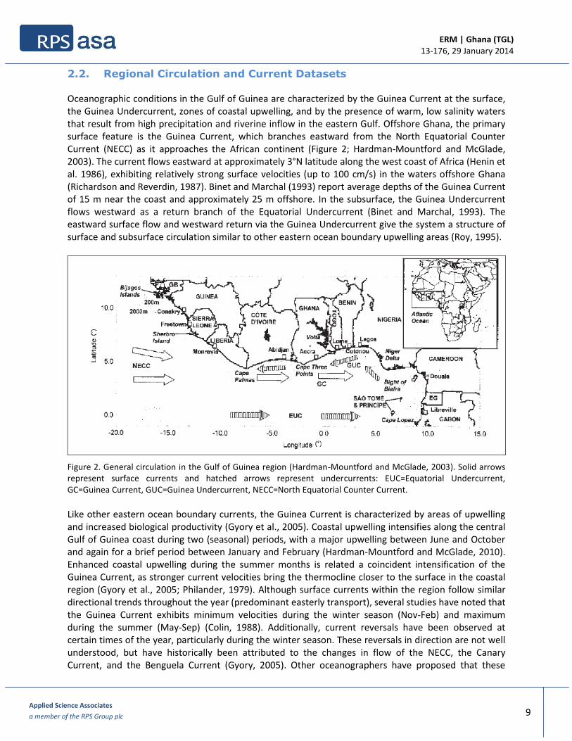
2.2. Regional Circulation and Current Datasets Oceanographic conditions in the Gulf of Guinea are characterized by the Guinea Current at the surface, the Guinea Undercurrent, zones of coastal upwelling, and by the presence of warm, low salinity waters that result from high precipitation and riverine inflow in the eastern Gulf. Offshore Ghana, the primary surface feature is the Guinea Current, which branches eastward from the North Equatorial Counter Current (NECC) as it approaches the African continent (Figure 2; Hardman-Mountford and McGlade, 2003). The current flows eastward at approximately 3°N latitude along the west coast of Africa (Henin et al. 1986), exhibiting relatively strong surface velocities (up to 100 cm/s) in the waters offshore Ghana (Richardson and Reverdin, 1987). Binet and Marchal (1993) report average depths of the Guinea Current of 15 m near the coast and approximately 25 m offshore. In the subsurface, the Guinea Undercurrent flows westward as a return branch of the Equatorial Undercurrent (Binet and Marchal, 1993). The eastward surface flow and westward return via the Guinea Undercurrent give the system a structure of surface and subsurface circulation similar to other eastern ocean boundary upwelling areas (Roy, 1995).

Figure 2. General circulation in the Gulf of Guinea region (Hardman-Mountford and McGlade, 2003). Solid arrows represent surface currents and hatched arrows represent undercurrents: EUC=Equatorial Undercurrent, GC=Guinea Current, GUC=Guinea Undercurrent, NECC=North Equatorial Counter Current.

Like other eastern ocean boundary currents, the Guinea Current is characterized by areas of upwelling and increased biological productivity (Gyory et al., 2005). Coastal upwelling intensifies along the central Gulf of Guinea coast during two (seasonal) periods, with a major upwelling between June and October and again for a brief period between January and February (Hardman-Mountford and McGlade, 2010). Enhanced coastal upwelling during the summer months is related a coincident intensification of the Guinea Current, as stronger current velocities bring the thermocline closer to the surface in the coastal region (Gyory et al., 2005; Philander, 1979). Although surface currents within the region follow similar directional trends throughout the year (predominant easterly transport), several studies have noted that the Guinea Current exhibits minimum velocities during the winter season (Nov-Feb) and maximum during the summer (May-Sep) (Colin, 1988). Additionally, current reversals have been observed at certain times of the year, particularly during the winter season. These reversals in direction are not well understood, but have historically been attributed to the changes in flow of the NECC, the Canary Current, and the Benguela Current (Gyory, 2005). Other oceanographers have proposed that these




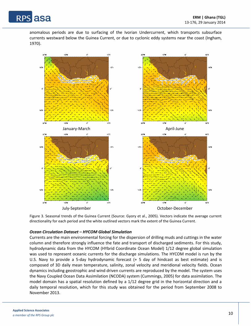
anomalous periods are due to surfacing of the Ivorian Undercurrent, which transports subsurface currents westward below the Guinea Current, or due to cyclonic eddy systems near the coast (Ingham, 1970).

January-March

April-June

July-September

October-December

Figure 3. Seasonal trends of the Guinea Current (Source: Gyory et al., 2005). Vectors indicate the average current directionality for each period and the white outlined vectors mark the extent of the Guinea Current.

Ocean Circulation Dataset – HYCOM Global Simulation Currents are the main environmental forcing for the dispersion of drilling muds and cuttings in the water column and therefore strongly influence the fate and transport of discharged sediments. For this study, hydrodynamic data from the HYCOM (HYbrid Coordinate Ocean Model) 1/12 degree global simulation was used to represent oceanic currents for the discharge simulations. The HYCOM model is run by the U.S. Navy to provide a 5-day hydrodynamic forecast (+ 5 day of hindcast as best estimate) and is composed of 3D daily mean temperature, salinity, zonal velocity and meridional velocity fields. Ocean dynamics including geostrophic and wind driven currents are reproduced by the model. The system uses the Navy Coupled Ocean Data Assimilation (NCODA) system (Cummings, 2005) for data assimilation. The model domain has a spatial resolution defined by a 1/12 degree grid in the horizontal direction and a daily temporal resolution, which for this study was obtained for the period from September 2008 to November 2013.




At each well site, daily currents were obtained by interpolating the values from the nearest HYCOM model grid point. At the model cell closest to En13-WI, the water column is represented in 26 discrete vertical layers; at En07-WI, the HYCOM model contains 24 vertical layers. Summary statistics from the hydrodynamic inputs are discussed further below, although at both sites the flow characteristics are quite similar. Vertical profiles derived from the nearest HYCOM model grid points show the average magnitude of currents with depth at each site (Figure 4 and Figure 5). Surface currents as represented by the model are of moderate speed (30-40 cm/s) although currents greater than 80 cm/s do occur approximately 5% of the time. Currents of this magnitude agree with observations of relatively strong surface velocities (~100 cm/s) in the surface waters offshore Ghana (Richardson and Reverdin, 1987). Current intensity decreases rapidly with depth in the water column and average speeds drop below 10 cm/s by 400 meters depth. Current roses showing the statistical distribution of modeled currents (by depth interval) indicate a cumulative easterly flow for surface currents. Bottom currents are directionally variable and extremely weak (average speeds between 2-3 cm/s). When viewed as monthly averages, statistics from the HYCOM dataset also reflect the seasonal variability in current speeds as noted above. Surface velocities are approximately 25% stronger during the boreal spring and summer Mar-Sep when compared to the annual average (Figure 6; Figure 7). The fastest surface velocities (>50 cm/s, on average) occur in April and May and the slowest (~25 cm/s) between during the winter months. Monthly current roses (Figure 8 and Figure 9) also indicate strong eastward flow during spring and summer months and weaker more variable currents during the fall/winter. By contrast, subsurface layers reach peak flow velocities during fall/winter months, although the difference in flow speeds is nominal (< 1 cm/s). Figure 10 and Figure 11 present time series (stick plots) of current vectors for the full HYCOM model period at En13-WI and En07-WI, respectively. The periodic flow reversals, and interannual variability in flow intensity represented in the model emphasize the complex spatial and temporal circulation patterns in the Gulf of Guinea, which are not fully represented in a regional flow schematic (e.g. Figure 2). At both locations, flow becomes more variable with depth and net westerly flow (attributed to the Guinea Undercurrent) is observed in the model at depths below 150 m. In the surface layers, the seasonal variability in currents are regular and repeatable features for all years in the time series and the dataset maintains these oscillations for depths above 50 m. As represented by the HYCOM model, currents have undergone intensification during the most recent calendar year (2013) and the dominant easterly-directed flow pattern is most apparent during this period. Bottom currents at both sites are characterized by generally weak and variable flow that persists year-round.




Figure 4. Vertical profile (left) and current roses showing the distribution of current speeds (right) for the En13-WI site, derived from HYCOM model currents between 2008 and 2013.




Figure 5. Vertical profile (left) and current roses showing the distribution of current speeds (right) for the En07-WI site, derived from HYCOM model currents between 2008 and 2013.




Figure 6. Monthly averaged current speeds at En13-WI derived from the HYCOM global dataset. Average current speeds are shown for the surface (top figure) and 1000 m (bottom figure) water depths.




Figure 7. Monthly averaged current speeds at En07-WI derived from the HYCOM global dataset. Average current speeds are shown for the surface (top figure) and 1000 m (bottom figure) water depths.




Figure 8. Current roses showing the distribution of surface currents (speed and direction) by month at the En13-WI site, derived from HYCOM model currents between 2008 and 2013.




Figure 9. Current roses showing the distribution of surface currents (speed and direction) by month at the En07-WI site, derived from HYCOM model currents between 2008 and 2013.




Figure 10. Time series of HYCOM model currents with depth at the En13-WI discharge site. Shading indicates the simulation periods (Apr 1-16 and Dec 1-16, 2012).




Figure 11. Time series of HYCOM model currents with depth at the En07-WI discharge site. Shading indicates the simulation periods (Apr 1-16 and Dec 1-16, 2012).




3. Drilling Discharge Simulations The following section describes the model used for simulating releases of drilling discharges and the release scenarios. Drilling discharges refers to waste materials and by-products of drilling that are often released directly to the marine environment, including drill cuttings and spent drilling muds. Because drilling is typically performed in different intervals (sections) reflecting differences in operations (drilling diameters), the discharge schedule may vary as a function of drilling rate, cuttings and mud volumes, or depth of release in the water column (near-surface or near-seabed typically). The analysis presented here evaluates differences in seabed deposition and sediment plume characteristics for a single discharge program released at two sites and over two different time periods (a total of four model scenarios).

3.1. Model Description - MUDMAP Drilling discharges simulations were completed using ASA’s MUDMAP modeling system (Spaulding et al., 1994). MUDMAP is a numerical model developed by ASA to predict the near and far field transport, dispersion, and bottom deposition of drilling mud and cuttings. In MUDMAP, the equations governing conservation of mass, momentum, buoyancy, and solid particle flux are formulated using integral plume theory and then solved using a Runge Kutta numerical integration technique. The model includes three stages: convective descent/ascent, dynamic collapse, and far field dispersion. It allows the transport and dispersion of the release to be modeled through all stages of its movement. The initial dilution and vertical spreading of the release is predicted in the convective descent/ascent process. The far field process predicts the transport and dispersion of the release caused by the ambient current and turbulence fields. In the dynamic collapse process, the release impacts the surface or bottom, or becomes trapped by vertical density gradients in the water column. The model output consists of definition of the movement and shape of the discharge plume, the concentrations of insoluble (i.e., cuttings and mud) discharge components in the water column, and the accumulation of discharged solids on the seabed. The model predicts the transport of discharged solids from the time of discharge to initial settling on the seabed. MUDMAP does not account for resuspension and transport of previously discharged solids; therefore it provides a conservative estimate of the potential seafloor depositions. The far field and passive diffusion stage is based on a particle based random walk model. More details about MUDMAP are included in Appendix A.

3.2. Discharge Scenarios Dispersion modeling was completed to evaluate seabed deposition and sediment plume extents resulting from discharges at the En13-WI and En07-WI drilling sites. Based on information provided by ERM/TGL, the drilling program at both sites consists of four sections; the first two sections to be drilled with water based mud (WBM) and the lowermost sections drilled using low toxicity oil based mud (LTOBM). The discharge schedule provided by ERM/TGL is shown in Table 2 and consists of the release of 1,643 Metric Tonnes (MT) of cuttings and 1,390 m3 of drilling fluids (WBM) over the course of 15 days. During the riserless phase of drilling (sections 1 and 2), all cuttings and WBM are expected to be released directly at the seabed (+5 m above the wellhead on the seafloor). Subsequent sections will be drilled with LTOBM and surface returns of cuttings will be processed with a thermal desorption unit (TDU) prior to discharge. The release of TDU powder was simulated from a depth of 15 meters below




the sea surface. A continuous discharge rate was specified for the duration of each of the individual drill sections. The release of drilling fluids from sections 3 and 4 was not simulated as it is expected that all LTOBM will be recovered and transported onshore for disposal. Table 2. Drilling discharges program used for model simulations at En13-WI and En07-WI.

Section Diameter

(in) Duration

(days) Cuttings Release

Rate (MT/hr) Mud Release Rate (m

3/hr)

Mud Type Drilling Start Date Release Depth

1

1 36” 0.5 11.46 15.83 WBM 1-Apr-12 1-Dec-12 seabed

2 26” 1.5 17.01 33.33 WBM 1-Apr-12 1-Dec-12 seabed

3 16” 6 4.8 — LTOBM 3-Apr-12 3-Dec-12 sea surface

4 12 ¼” 7 1.2 — LTOBM 9-Apr-12 9-Dec-12 sea surface

Total Discharges 1,642.68 MT 1,389.84 m3

1 releases simulated at 5 m above the seabed and 15 m below the sea surface

Because currents are the main driving force for the transport and dispersion of discharged drilling muds and cuttings in the water column, seasonal, annual, or interannual variability in currents can strongly influence the fate of discharged material. Analysis of hydrodynamic model data (Section 2.2) suggests that currents in the region are complex and undergo substantial variability both spatially and temporally. Because drilling operations within the DWT Block will occur throughout the year, a modeling strategy was developed to compare the results of different flow conditions that characterize the potential range of release periods. Seasonal differences in the current field were represented by simulating releases during the months of April and December -- periods identified during previous modeling for the TEN Development (ASA project 11-053). Drilling releases were simulated to begin on April 1, a period of peak surface current velocities that are directed primarily toward the east. An additional model of the same duration was run with discharges beginning on December 1, a period characterized by less intense currents in upper water column that are more directionally variable. For both periods, subsurface currents (below 500 m) are relatively weak (<8 cm/s). In total, four (4) discharge scenarios were performed using the MUDMAP dispersion model representing both discharge programs simulated at different times of the year. For all scenarios, vertically and time varied currents derived from HYCOM for a representative period (2012-2013) were used to drive the advection of the discharged solids. The exact HYCOM currents used for modeling correspond to the dates shown in Table 2.

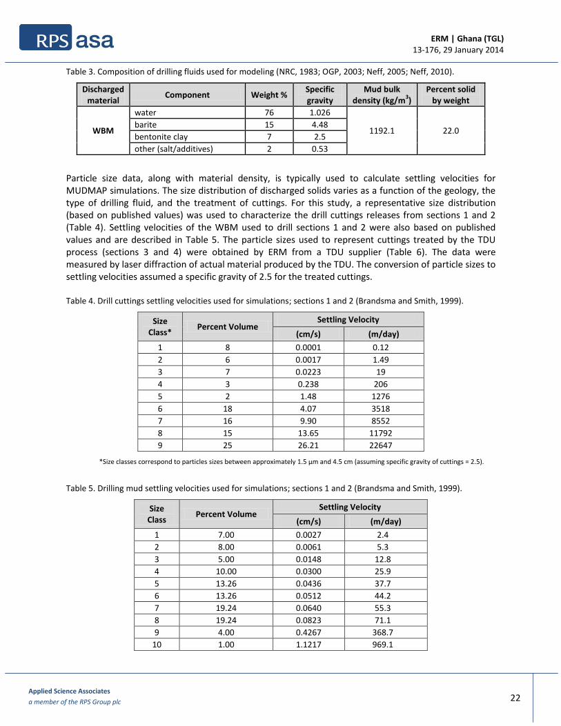
3.3. Discharge sediment characteristics To assess the fate of drilling discharges in the marine environment it is critical to characterize the components of the released materials. The composition of the drilling mud applied will depend on the characteristics of the formation and this composition determines the density and weight of the discharged fluid, its toxicity, and the settling velocities of the material released in the water column. Information describing the specific components of the drilling mud expected to be used for operations within the Enyenra field (including the percent water and concentration and type of weighting materials) was not provided with the discharge schedule. For this reason, a representative WBM fluid composition was assumed for modeling. The composition (in weight percent) for the various components of typical drilling muds is presented in Table 3. The bulk density of the drilling fluids used for MUDMAP simulations was 1,192.1 kg/m3. Solid particles occupy 22% of the total mud weight.




Table 3. Composition of drilling fluids used for modeling (NRC, 1983; OGP, 2003; Neff, 2005; Neff, 2010).

Discharged material

Component Weight % Specific gravity

Mud bulk density (kg/m

3)

Percent solid by weight

WBM

water 76 1.026

1192.1 22.0 barite 15 4.48

bentonite clay 7 2.5

other (salt/additives) 2 0.53

Particle size data, along with material density, is typically used to calculate settling velocities for MUDMAP simulations. The size distribution of discharged solids varies as a function of the geology, the type of drilling fluid, and the treatment of cuttings. For this study, a representative size distribution (based on published values) was used to characterize the drill cuttings releases from sections 1 and 2 (Table 4). Settling velocities of the WBM used to drill sections 1 and 2 were also based on published values and are described in Table 5. The particle sizes used to represent cuttings treated by the TDU process (sections 3 and 4) were obtained by ERM from a TDU supplier (Table 6). The data were measured by laser diffraction of actual material produced by the TDU. The conversion of particle sizes to settling velocities assumed a specific gravity of 2.5 for the treated cuttings. Table 4. Drill cuttings settling velocities used for simulations; sections 1 and 2 (Brandsma and Smith, 1999).

Size Class*

Percent Volume Settling Velocity

(cm/s) (m/day)

1 8 0.0001 0.12

2 6 0.0017 1.49

3 7 0.0223 19

4 3 0.238 206

5 2 1.48 1276

6 18 4.07 3518

7 16 9.90 8552

8 15 13.65 11792

9 25 26.21 22647

*Size classes correspond to particles sizes between approximately 1.5 μm and 4.5 cm (assuming specific gravity of cuttings = 2.5).

Table 5. Drilling mud settling velocities used for simulations; sections 1 and 2 (Brandsma and Smith, 1999).

Size Class


(cm/s) (m/day)

1 7.00 0.0027 2.4

2 8.00 0.0061 5.3

3 5.00 0.0148 12.8

4 10.00 0.0300 25.9

5 13.26 0.0436 37.7

6 13.26 0.0512 44.2

7 19.24 0.0640 55.3

8 19.24 0.0823 71.1

9 4.00 0.4267 368.7

10 1.00 1.1217 969.1




Table 6. TDU cuttings settling velocities used for simulations; sections 3 and 4 (sourced from TDU supplier).

Size Class


(cm/s) (m/day)

1 3.46 0.000034 0.028977

2 4.35 0.000042 0.036482

3 4.95 0.000053 0.045989

4 4.86 0.000067 0.057872

5 4.22 0.000084 0.072858

6 3.46 0.000106 0.091748

7 2.82 0.000134 0.115518

8 2.42 0.000168 0.145348

9 2.22 0.000212 0.182976

10 2.20 0.000267 0.230388

11 2.28 0.000336 0.289992

12 2.43 0.000423 0.365146

13 2.60 0.000532 0.459744

14 2.73 0.00067 0.578778

15 2.82 0.000843 0.728321

16 2.86 0.001062 0.917166

17 2.86 0.001336 1.154635

18 2.84 0.001683 1.453683

19 2.81 0.002118 1.829683

20 2.80 0.002666 2.303524

21 2.83 0.003357 2.900284

22 2.87 0.004226 3.651159

23 2.95 0.00532 4.596443

24 3.04 0.006697 5.786267

25 3.10 0.008431 7.284735

26 3.14 0.01061 9.17133

27 3.10 0.01336 11.54536

28 3.00 0.01682 14.53478

29 2.81 0.02118 18.29761

30 2.54 0.02666 23.03698

31 2.19 0.03357 29.00121

32 1.82 0.04226 36.51004

33 1.43 0.0532 45.96408

34 1.80 0.08431 72.84509

35 1.15 0.2118 182.9837

36 0.24 0.532 459.628

The extent to which discharged sediments accumulate on the seabed is largely controlled by the particle settling velocities (a function of size and density) and the prevailing currents in the water column. Figure 12 compares settling characteristics for each of the discharged materials used as model input. Given the relatively deep water at both drilling sites (>1,000 m), and the fine particle sizes resulting from the TDU treatment process, releases near the seabed are expected to contribute more substantially to deposition as compared to those occurring at the surface. Not taking into account the advective processes, over 85% of the TDU powder would require at least 10 days in order to settle from the surface to the seabed at En-13.




Figure 12. Comparison of settling velocities for solid discharges used in the modeling study. Size class divisions are from Gibbs et al. (1971).




4. Results of the Drilling Discharge Simulations

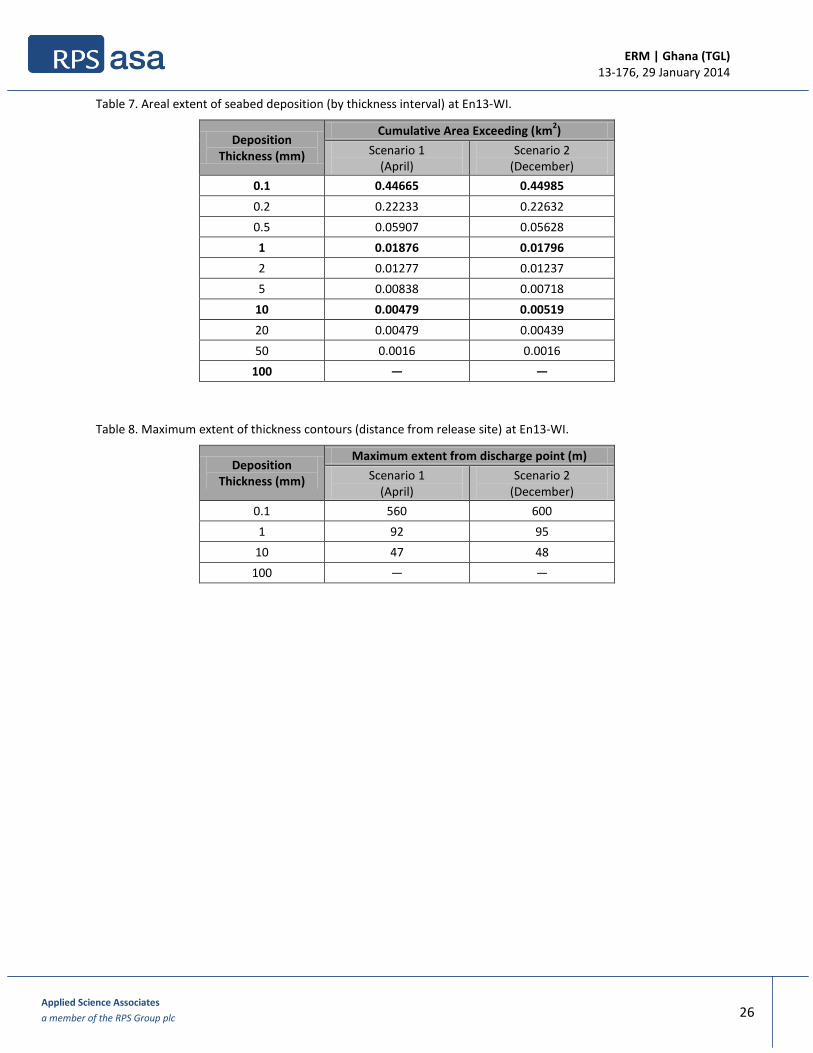
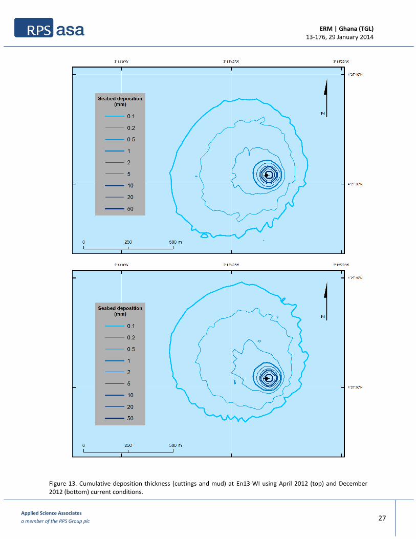
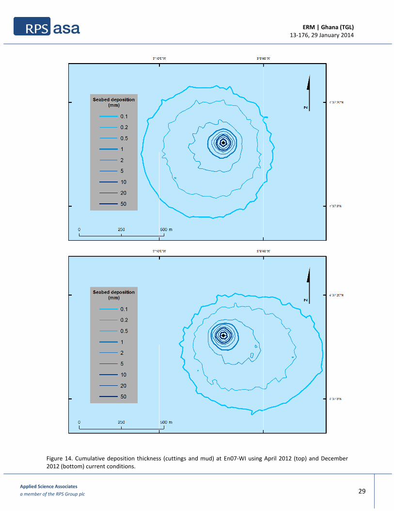
4.1. Predicted deposition thickness Four discharge scenarios were analysed, corresponding to the schedules and release volumes described in Section 3.2. MUDMAP was used to predict the resulting bottom deposition from each discharge along with the pattern of cumulative deposits. Following the simulated release of each section in MUDMAP, the model continued to track the far field dispersion for four additional days, to account for the settling of fine material suspended in the water column. Figure 13 and Figure 14 show the plan view extents of the model-predicted seabed deposition at En13-WI and En07-WI, respectively; Table 7 through Table 10 summarizes the areal impact of each scenario. As shown in Figure 13 and Figure 14, the extent of deposition between sites and between seasons is nominal. All scenarios result in a generally rounded and tight depositional footprint that surrounds the well head. Contours representing very fine thickness intervals (0.1 mm) are slightly more elongate and extend between 505 m and 620 m from the release sites. Deposit thicknesses for each scenario are calculated from mass accumulation on the seabed and assume a sediment bulk density of 2,500 kg/m3 and no void ratio (zero porosity). Differences in the extent of deposition between each season are primarily confined to thicknesses below 1 mm. For both sites, the most substantial differences are in the orientation of the very fine deposition defined by the 0.5-0.1 mm contours. Although the areal extent of these intervals remains similar between the discharge periods (Figure 15 and Figure 16), the overall shape is indicative of the flow characteristics at depth during the seabed releases. For all scenarios, the gradient of contours at or above 1 mm is uniform and concentric around the well, which indicates that dispersion processes are nearly as influential as advection from currents due to the settling characteristics of material being released and the water depths. When drilling occurs in deep water (> 1000 m), which is the case for both the En13-WI and En07-WI well sites, discharges originating from the sea surface may not contribute substantially to the observed deposition at the seafloor. For this study, the extremely fine particle sizes of the TDU powder further contribute to this outcome. At both sites, the TDU powder discharges remain suspended in the upper water column until eventually dispersing below levels detectible by the model. As a consequence, the surface releases do not contribute significantly to the cumulative mass accumulation on the seabed. By contrast, the cuttings discharged directly at the seabed (sections 1 and 2) settle relatively quickly owing to (i) the release depth, (ii) the size distribution, and (iii) the relatively weak currents near the seabed. Seabed releases of WBM are transported further from the discharge site by the prevailing currents resulting in the broad, thin deposition layers. At the En13-WI drilling site, the discharge program results in deposition of 10 mm up to 48 m from the well and an aerial extent of 0.00519 km2; deposition at 1 mm extends a maximum of 95 m and covers an area of 0.01876 km2; and deposition at thickness of 0.1 mm extends a maximum of 600 m and covers 0.44985 km2 of the seabed. At En07-WI, thicknesses of 10 mm or greater are confined to a distance of 47 m from the discharge site and an aerial extent of 0.00599 km2; deposition at 1 mm extends a maximum of 96 m and covers an area of 0.02195 km2; and deposition at thickness of 0.1 mm extends 620 m and covers up to 0.471 km2of the seabed.




Table 7. Areal extent of seabed deposition (by thickness interval) at En13-WI.

Deposition Thickness (mm)

Cumulative Area Exceeding (km2)

Scenario 1 (April)

Scenario 2 (December)

0.1 0.44665 0.44985

0.2 0.22233 0.22632

0.5 0.05907 0.05628

1 0.01876 0.01796

2 0.01277 0.01237

5 0.00838 0.00718

10 0.00479 0.00519

20 0.00479 0.00439

50 0.0016 0.0016

100 — —

Table 8. Maximum extent of thickness contours (distance from release site) at En13-WI.


Maximum extent from discharge point (m)

Scenario 1 (April)


0.1 560 600

1 92 95

10 47 48

100 — —




Figure 13. Cumulative deposition thickness (cuttings and mud) at En13-WI using April 2012 (top) and December 2012 (bottom) current conditions.




Table 9. Areal extent of seabed deposition (by thickness interval) at En07-WI.


Cumulative Area Exceeding (ha)

Scenario 1 (April)


0.1 0.471 0.44705

0.2 0.25426 0.23311

0.5 0.07185 0.05987

1 0.02195 0.01876

2 0.01317 0.01197

5 0.00758 0.00798

10 0.00599 0.00519

20 0.00319 0.00399

50 0.0012 0.0016

100 — 0.44705

Table 10. Maximum extent of thickness contours (distance from release site) at En07-WI.


Maximum extent from discharge point (m)

Scenario 1 (April)


0.1 505 620

1 96 93

10 47 46

100 — —




Figure 14. Cumulative deposition thickness (cuttings and mud) at En07-WI using April 2012 (top) and December 2012 (bottom) current conditions.




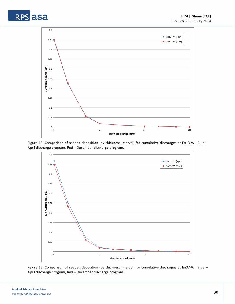
Figure 15. Comparison of seabed deposition (by thickness interval) for cumulative discharges at En13-WI. Blue – April discharge program, Red – December discharge program.

Figure 16. Comparison of seabed deposition (by thickness interval) for cumulative discharges at En07-WI. Blue – April discharge program, Red – December discharge program.




4.2. Predicted Water Column Concentrations MUDMAP was also used to predict concentrations of total suspended solids (TSS) in the water column as a result of discharges at the sea surface. As discussed in section 4.1, a significant portion of TDU powder released from the MODU remains suspended in the water column. Any sustained water column plumes are controlled by currents at the sea surface and by the rate that the TDU powder is released. Thus, to reproduce maximum TSS concentrations, simulations were performed for the drilling interval corresponding to the largest release rate (section 3; Table 2). Drilling in the Enyenra field is expected to occur throughout the year. Accordingly a total of eight representative MUDMAP scenarios were performed to evaluate the range in extent and trajectory of the sediment plume as a result of variability in currents, seasons, and drilling sites. Table 11 summarizes the inputs for each model run. For each scenario, the release of TDU powder was simulated for approximately four hours, allowing the water column to achieve steady state concentrations of suspended sediments. For each scenario the model then continued to track the transport and dispersion of the plume until its maximum concentrations declined below 10 mg/L. 10 mg/L was selected as a background concentration based on an environmental baseline survey of the adjacent Jubilee field (TDI-Brooks, 2008), which indicates that minimum concentrations of suspended solids in the region are 11.22 mg/L.

Table 11. Date, release rate, and current regime used to calculate the maximum TSS concentrations for each release scenario.

Name Scenario Discharge Date Drilling Section

Release Rate (MT/hr)

Scenario 1 Maximum current speeds, EN13-WI

April 2012 8 April 2012 3 (16”) 4.8

Scenario 2 Minimum current speeds, EN13-WI

April 2012 27 April 2012 3 (16”) 4.8

Scenario 3 Maximum current speeds, EN13-WI December 2012

14 December 2012 3 (16”) 4.8

Scenario 4 Minimum current speeds, EN13-WI December 2012

4 December 2012 3 (16”) 4.8

Scenario 5 Maximum current speeds, EN07-WI

April 2012 9 April 2012 3 (16”) 4.8

Scenario 6 Minimum current speeds, EN07-WI

April 2012 30 April 2012 3 (16”) 4.8

Scenario 7 Maximum current speeds, EN07-WI December 2012

16 December 2012 3 (16”) 4.8

Scenario 8 Minimum current speeds, EN07-WI December 2012

28 December 2012 3 (16”) 4.8




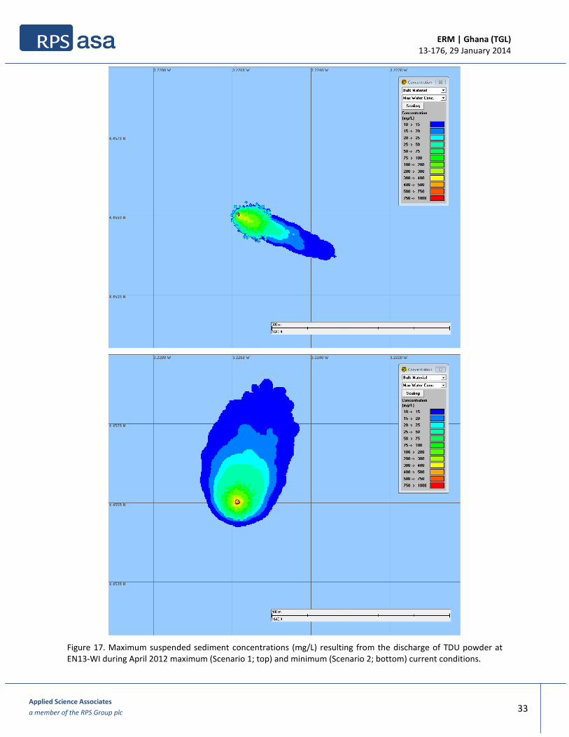
Figure 17 through Figure 20 show the aggregation of TSS values that occur for the duration each simulation. These figures do not represent any instantaneous snapshot of water column concentrations, but instead show the maximum, time-integrated TSS within the study domain for each modeled release. The maximum predicted concentration of suspended sediments in the water column ranges from a maximum of 896 mg/L as a result of discharges at En07-WI during December (Scenario 8), to 467 mg/L at En13-WI during April (Scenario 1). Due to the small particle sizes that result from the TDU treatment process and the relatively strong current speeds at the surface, most of the suspended sediment remains within the uppermost 30 meters of the water column until dispersing below the 10 mg/L threshold. Table 12 summarizes the maximum distance of observed excess water column concentrations for each of the eight scenarios. The trends observed in the model-predicted TSS plume are similar to those of the seabed deposition simulations; namely, that the plume trajectory varies as a result of the flow regime occurring on the day of the release. For that reason the results should be considered within the context of all possible current conditions in the DWT block. In general, the extent of the plumes is greater during strong current conditions, while the maximum TSS concentrations increase during weak current conditions and persist for longer in the water column. For all scenarios, the plume migrates from the release site immediately after drilling discharges cease. The plume travels with ambient currents until dispersion and turbulence cause the TSS concentrations to fall below the 10 mg/L threshold. To this end, a stronger current regime has the effect of clearing the water column more quickly than weaker and more variable flow, although in all cases, the water column returns to ambient conditions (<10 mg/L) within an hour of the final release. Very strong surface currents (such as those that correspond with Scenario 1; >100 cm/s) allow the model domain to achieve background concentrations in less than 10 minutes. The threshold of 10 mg/L reflects a conservative estimate of ambient TSS concentrations based on previous field investigations offshore Ghana (TDI-Brooks, 2008). Table 12. Maximum distance of excess water column concentrations for each discharge scenario.

Water Column Concentration

(mg/L)

Distance from discharge point (m)

Scenario 1 Scenario 2 Scenario 3 Scenario 4 Scenario 5 Scenario 6 Scenario 7 Scenario 8

10 302 355 312 230 325 360 309 340

50 99 62 78 55 88 59 72 57

100 75 41 59 37 62 42 45 41

500 — 8 6 8 — 7 7 8




Figure 17. Maximum suspended sediment concentrations (mg/L) resulting from the discharge of TDU powder at EN13-WI during April 2012 maximum (Scenario 1; top) and minimum (Scenario 2; bottom) current conditions.




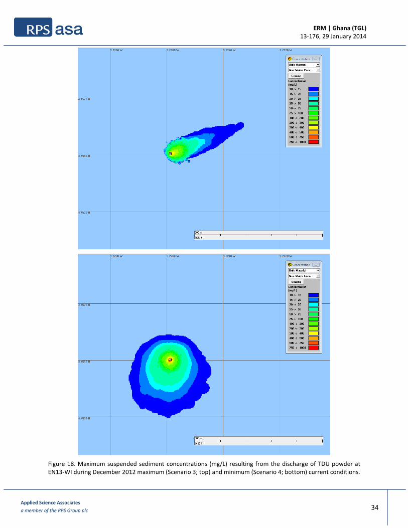
Figure 18. Maximum suspended sediment concentrations (mg/L) resulting from the discharge of TDU powder at EN13-WI during December 2012 maximum (Scenario 3; top) and minimum (Scenario 4; bottom) current conditions.




Figure 19. Maximum suspended sediment concentrations (mg/L) resulting from the discharge of TDU powder at EN07-WI during April 2012 maximum (Scenario 5; top) and minimum (Scenario 6; bottom) current conditions.




Figure 20. Maximum suspended sediment concentrations (mg/L) resulting from the discharge of TDU powder at EN07-WI during December 2012 maximum (Scenario 7; top) and minimum (Scenario 8; bottom) current conditions.




5. Conclusions This report presents the results of drill cuttings and mud discharge simulations conducted for two locations in the Deepwater Tano Block, in the Gulf of Guinea. The drilling sites (En07-WI and En13-WI) are situated along the continental slope, approximately 50-70 km south of the Ghanaian coastline, and 2-4 km from the maritime boundary with Côte d’Ivoire. Dispersion modeling was completed at both sites in order to evaluate seabed deposition from releases of drilling mud and cuttings and the potential for sediment plumes resulting from the discharge of pulverized cuttings after treatment with a thermal desorption unit. Simulations of drilling releases were completed using ASA’s MUDMAP modeling software. Because drilling operations within the DWT block are expected to occur throughout the year, a modeling strategy was developed to compare the results of different flow conditions that characterize the potential range of release periods. Specifically, releases were simulated during the months of April and December – which were identified as representative periods during previous modeling for the TEN Development. A total of four discharge scenarios were performed to evaluate seabed deposition (2 release periods per location). An additional eight MUDMAP simulations were performed to examine the range in plume characteristics from sea surface discharges (2 sites x 2 periods x 2 current regimes). For each scenario, vertically and time varied currents derived from the HYCOM 1/12 degree global simulation for a representative period (2012-2013) were used to drive the advection of the discharged solids. The cumulative seabed deposition resulting from each discharge scenario was analysed along with predictions of suspended sediment plumes in the upper water column resulting from the near-instantaneous release of drilling mud. In summary:

All scenarios result in a generally rounded and tight depositional footprint that surrounds each well head. Contours representing very fine thickness intervals (0.1 mm) are slightly more elongate and extend between 505 m and 620 m from the release sites. The areal extent of deposition above 1 mm is nearly indistinguishable between sites/seasons.

Because both sites utilize the same discharge schedule, differences in the extent of seabed deposition between sites and seasons is nominal. This is primarily due to the occurrence of very weak bottom currents at both sites, and the treatment of cuttings returned to the MODU. The TDU process results in extremely fine particles that not contribute significantly to the cumulative mass accumulation on the seabed.

Thicknesses at or above 1 mm are confined to an area within 96 m of the well head and thickness greater than 10 mm are confined to 48 m.

Sediment plumes resulting from discharges of TDU powder are predicted to extend between 230 and 360 m from the release site; the trajectory varies as a result of the flow regime occurring on the day of the release.

In general, the extent of the plumes is greater during strong current conditions, while the maximum TSS concentrations increase during weak current conditions and persist for longer in the water column. The maximum predicted concentration of suspended sediments in the water column (corresponding to the weakest current regime) is 896 mg/L.

In all cases, the water column is predicted to return to ambient conditions (<10 mg/L) within an hour of the final release.




6. References Binet, D. and Marchal, E., 1993. The Large Marine Ecosystem of the Gulf of Guinea: long term variability

induced by climatic changes. In Large Marine Ecosystems—Stress, Mitigation and Sustainability, edited by K. Sherman, L. M. Alexander and B. Gold (Washington, DC: American Association for the Advancement of Science), pp. 104–118.

Brandsma, M.G. & Smith, J.P., 1999. Offshore Operators Committee mud and produced water discharge

model – report and user guide. Exxon Production Research Company, December 1999. Cohn, N., Isaji, T. Mulanaphy, N., Geiger, E., and Comerma, E., 2012. Oil Spill, Drilling Discharge, and

Produced Water Modelling, TEN Development, Offshore Ghana. ASA project 11-053. Colin, C., 1988. Coastal upwelling events in front of Ivory Coast during the FOCAL program. Oceanologia

Acta, v. 11, 125-138. Cummings, J.A., 2005: Operational multivariate ocean data assimilation. Quart. J. Royal Met. Soc., Part C,

131(613), 3583-3604. Gibbs, R.J., Matthews, M.D. and Link, D.A., 1971. The relationship between sphere size and settling

velocity. Journal of Sedimentary Research, v. 41, 7-18. Gyory J., Bischof, B., Marian, A.J., and Ryan, E.H., 2005. The Guinea Current. Ocean Surface Currents.

http://oceancurrents.rsmas.miami.edu/atlantic/guinea.html. Hardman-Mountford, N.J., and McGlade, J.M., 2003. Seasonal and interannual variability of

oceanographic processes in the Gulf of Guinea: An investigation using AVHRR sea surface temperature data. International Journal of Remote Sensing. v. 24. 3247–3268.

Henin, C., P. Hisard, and B. Piton, 1986. Observations hydrologiques dans l'ocean Atlantique Equatorial,

Ed. ORSTOM, FOCAL, v. 1, 1-191. Ingham, M.C., 1970. Coastal upwelling in the northwestern gulf of Guinea. Bulletin of Marine Science, v.

20, 1-34. International Association of Oil and Gas Producers (OGP), 2003. Environmental aspects of the use and

disposal of non aqueous drilling fluids associated with offshore oil & gas operations. Report No. 342. 104 pp.

National Research Council (NRC), 1983. Drilling discharges in the marine environment. National

Academy Press. Washington D. C. 195 pp. Neff, J.M., 2005. Composition, environmental fates, and biological effect of water based drilling muds

and cuttings discharged to the marine environment: A synthesis and annotated bibliography. Prepared for Petroleum Environmental Research Forum (PERF) and American Petroleum Institute by Battelle. Duxbury, MA. 73 pp.




Neff, J.M., 2010. Fates and effects of water based drilling muds and cuttings in cold-water environments. Prepared for Shell Exploration and Production Company by Neff & Associates LLC. Duxbury, MA. 287 pp.

Philander, S.G.H., 1979. Upwelling in the Gulf of Guinea. Journal of Marine Research, v. 37, 23-33. Richardson, P.L. and G. Reverdin, 1987: Seasonal cycle of velocity in the Atlantic North Equatorial

Countercurrent as measured by surface drifters, current meters, and ship drifts. Journal of Geophysical Research, v. 92, 3691-3708.

Roy, C., 1995. The Cote d’Ivoire and Ghana coastal upwellings: Dynamics and changes. In Dynamics and

Use of Sardinella Resources from Upwelling off Ghana and Ivory Coast, edited by F. X. Bard and K. A. Koranteng (Paris: ORSTOM Editions), pp. 346–361.

Spaulding, M. L., T. Isaji, and E. Howlett. 1994. MUDMAP: A model to predict the transport and

dispersion of drill muds and production water. Applied Science Associates, Inc, Narragansett, RI. TDI-Brooks (2008). Jubilee field Ghana Environmental Baseline Survey Report. Technical Report # 08-

2161 Texas, USA.




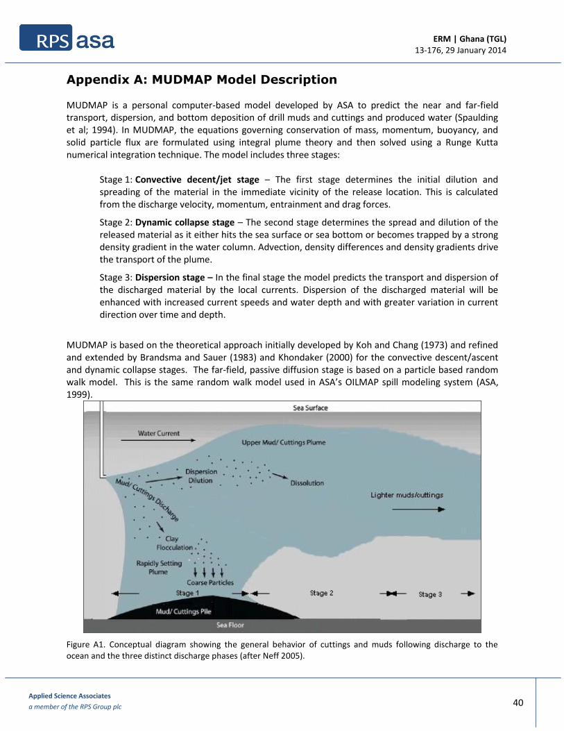
Appendix A: MUDMAP Model Description MUDMAP is a personal computer-based model developed by ASA to predict the near and far-field transport, dispersion, and bottom deposition of drill muds and cuttings and produced water (Spaulding et al; 1994). In MUDMAP, the equations governing conservation of mass, momentum, buoyancy, and solid particle flux are formulated using integral plume theory and then solved using a Runge Kutta numerical integration technique. The model includes three stages:

Stage 1: Convective decent/jet stage – The first stage determines the initial dilution and spreading of the material in the immediate vicinity of the release location. This is calculated from the discharge velocity, momentum, entrainment and drag forces.

Stage 2: Dynamic collapse stage – The second stage determines the spread and dilution of the released material as it either hits the sea surface or sea bottom or becomes trapped by a strong density gradient in the water column. Advection, density differences and density gradients drive the transport of the plume.

Stage 3: Dispersion stage – In the final stage the model predicts the transport and dispersion of the discharged material by the local currents. Dispersion of the discharged material will be enhanced with increased current speeds and water depth and with greater variation in current direction over time and depth.

MUDMAP is based on the theoretical approach initially developed by Koh and Chang (1973) and refined and extended by Brandsma and Sauer (1983) and Khondaker (2000) for the convective descent/ascent and dynamic collapse stages. The far-field, passive diffusion stage is based on a particle based random walk model. This is the same random walk model used in ASA’s OILMAP spill modeling system (ASA, 1999).

Figure A1. Conceptual diagram showing the general behavior of cuttings and muds following discharge to the ocean and the three distinct discharge phases (after Neff 2005).




The model’s output consists of calculations of the movement and shape of the discharge plume, the concentrations of soluble (i.e. oil in produced water) and insoluble (i.e. cuttings and muds) discharge components in the water column, and the accumulation of discharged solids on the seabed. The model predicts the initial fate of discharged solids, from the time of discharge to initial settling on the seabed As MUDMAP does not account for resuspension and transport of previously discharged solids, it provides a conservative estimate of the potential seafloor concentrations (Neff 2005).

Figure A2 Example MUDMAP bottom concentration output for drilling fluid discharge.

Figure A3. Example MUDMAP water column concentration output for drilling fluid discharge.




MUDMAP uses a color graphics-based user interface and provides an embedded geographic information system, environmental data management tools, and procedures to input data and to animate model output. The system can be readily applied to any location in the world. Application of MUDMAP to predict the transport and deposition of heavy and light drill fluids off Pt. Conception, California and the near-field plume dynamics of a laboratory experiment for a multi-component mud discharged into a uniform flowing, stratified water column are presented in Spaulding et al. (1994). King and McAllister (1997, 1998) present the application and extensive verification of the model for a produced water discharge on Australia’s northwest shelf. GEMS (1998) applied the model to assess the dispersion and deposition of drilling cuttings released off the northwest coast of Australia. MUDMAP References Applied Science Associates, Inc. (ASA), 1999. OILMAP technical and user’s manual, Applied Science

Associates, Inc., Narragansett, RI.

Brandsma, M.G., and T.C. Sauer, Jr., 1983. The OOC model: prediction of short term fate of drilling mud in the ocean, Part I model description and Part II model results. Proceedings of Workshop on an Evaluation of Effluent Dispersion and Fate Models for OCS Platforms, Santa Barbara, California.

GEMS - Global Environmental Modelling Services, 1998. Quantitative assessment of the dispersion and seabed depositions of drill cutting discharges from Lameroo-1 AC/P16, prepared for Woodside Offshore Petroleum. Prepared by Global Environmental Modelling Services, Australia, June 16, 1998.

King, B., and F.A. McAllister, 1997. Modelling the dispersion of produced water discharge in Australia, Volume I and II. Australian Institute of Marine Science report to the APPEA and ERDC.

King, B., and F.A. McAllister, 1998. Modelling the dispersion of produced water discharges. APPEA Journal 1998, pp. 681-691.

Koh, R.C.Y., and Y.C. Chang, 1973. Mathematical model for barged ocean disposal of waste. Environmental Protection Technology Series EPA 660/2-73-029, U.S. Army Engineer Waterways Experiment Station, Vicksburg, Mississippi.

Khondaker, A. N., 2000. Modelling the fate of drilling waste in marine environment – an overview. Journal of Computers and Geosciences Vol. 26, pp. 531-540.

Neff, J., 2005. Composition, environment fates, and biological effect of water based drilling muds and cuttings discharged to the marine environment: A synthesis and annotated bibliography. Report prepared for Petroleum Environment Research Forum and American Petroleum Institute.

Spaulding, M. L., T. Isaji, and E. Howlett, 1994. MUDMAP: A model to predict the transport and dispersion of drill muds and production water, Applied Science Associates, Inc, Narragansett, RI.

draft report dispersion modeling of drilling applied

Documents