draft - ats-lang.sourceforge.net

DR

AFTThe ATS Programming Language

(ATS/Anairiats User’s Guide)

(Started on the 16th of July, 2008)

(Working Draft of October 22, 2010)

Hongwei Xi

Boston University

Copyright c©2008–20??All rights reserved

DR

AFT

This manual documents ATS/Anairiats version x.x.x, which is the current released implementa-

tion of the programming language ATS. This implementation itself is nearly all written in ATS.

The core of ATS is a call-by-value functional programming language equipped with a type

system rooted in the framework Applied Type System (Xi, 2004). In particular, both dependent

types and linear types are supported in ATS. The dependent types in ATS are directly based on those

developed in Dependent ML (DML), an experimental programming language that is designed in an

attempt to extend ML with support for practical programming with dependent types (Xi, 2007). As

of now, ATS fully supersedes DML. While the notion of linear types is a familiar one in programming

lanugage research, the support for practical programming with linear types in ATS is unique: It is

based on a programming paradigm in which programming is combined with theorem-proving.

The type system of ATS is stratified, consisting of a static component (statics) and a dynamic

component (dynamics). Types are formed and reasoned about in the statics while programs are

constructed and evaluated in the dynamics. There is also a theorem-proving system ATS/LF built

within ATS, which plays an indispensable role in supporting the paradigm of programming with

theorem-proving. ATS/LF can also be employed to encode various deduction systems and their

meta-properties.

There is no support for program extraction (from proofs) in ATS. Instead, the ATS compiler

(Anairiats) erases all the types and proofs contained in a program after it passes typechecking, and

then translates the obtained erasure into C code that can be further compiled into object code by a

C compiler such as GCC.

ATS programs can run with or without run-time garbage collection. The time and space effi-

ciency of the C code generated from a program written in ATS often rivals that of its counterpart

written in C (or C++) directly. This is of particular importance when ATS is used for systems

programming.

DR

AFTContents

1 ATS BASICS 5

1.1 A Simple Example: Hello, world! . . . . . . . . . . . . . . . . . . . . . . . . . . . . 5

1.2 Elements of Programming . . . . . . . . . . . . . . . . . . . . . . . . . . . . . . . . 6

1.2.1 Comments . . . . . . . . . . . . . . . . . . . . . . . . . . . . . . . . . . . . . 6

1.2.2 Primitive Expressions . . . . . . . . . . . . . . . . . . . . . . . . . . . . . . . 7

1.2.3 Fixity . . . . . . . . . . . . . . . . . . . . . . . . . . . . . . . . . . . . . . . 7

1.2.4 Naming and the Environment . . . . . . . . . . . . . . . . . . . . . . . . . . 8

1.2.5 Conditionals . . . . . . . . . . . . . . . . . . . . . . . . . . . . . . . . . . . 9

1.2.6 Local Bindings . . . . . . . . . . . . . . . . . . . . . . . . . . . . . . . . . . 9

1.2.7 Function Definitions . . . . . . . . . . . . . . . . . . . . . . . . . . . . . . . 10

1.2.8 Overloading . . . . . . . . . . . . . . . . . . . . . . . . . . . . . . . . . . . . 10

1.3 Tuples and Records . . . . . . . . . . . . . . . . . . . . . . . . . . . . . . . . . . . . 11

1.4 Disjoint Variants . . . . . . . . . . . . . . . . . . . . . . . . . . . . . . . . . . . . . 12

1.5 Parametric Polymorphism and Templates . . . . . . . . . . . . . . . . . . . . . . . . 13

1.5.1 Template Declaration and Implementation . . . . . . . . . . . . . . . . . . . 14

1.6 Lists . . . . . . . . . . . . . . . . . . . . . . . . . . . . . . . . . . . . . . . . . . . . 15

1.7 Exceptions . . . . . . . . . . . . . . . . . . . . . . . . . . . . . . . . . . . . . . . . . 15

1.8 References . . . . . . . . . . . . . . . . . . . . . . . . . . . . . . . . . . . . . . . . . 16

1.9 Arrays . . . . . . . . . . . . . . . . . . . . . . . . . . . . . . . . . . . . . . . . . . . 17

1.10 Higher-Order Functions . . . . . . . . . . . . . . . . . . . . . . . . . . . . . . . . . 17

1.11 Tail-Call Optimization . . . . . . . . . . . . . . . . . . . . . . . . . . . . . . . . . . 18

1.12 Static and Dynamic Files . . . . . . . . . . . . . . . . . . . . . . . . . . . . . . . . . 20

1.13 Static Load and Dynamic Load . . . . . . . . . . . . . . . . . . . . . . . . . . . . . . 21

1.14 Input and Output . . . . . . . . . . . . . . . . . . . . . . . . . . . . . . . . . . . . . 21

1.15 A Simple Package for Rational Numbers . . . . . . . . . . . . . . . . . . . . . . . . 23

2 BATCH COMPILATION 27

2.1 The Command atsopt . . . . . . . . . . . . . . . . . . . . . . . . . . . . . . . . . . . 27

2.1.1 Compiling Static and Dynamic Files . . . . . . . . . . . . . . . . . . . . . . . 27

2.1.2 Typechecking Only . . . . . . . . . . . . . . . . . . . . . . . . . . . . . . . . 28

2.1.3 Generating HTML Files . . . . . . . . . . . . . . . . . . . . . . . . . . . . . . 28

2.1.4 Generating HTML Files for cross-referencing . . . . . . . . . . . . . . . . . . 28

2.1.5 Generating Usage Information . . . . . . . . . . . . . . . . . . . . . . . . . . 28

2.1.6 Generating Version Information . . . . . . . . . . . . . . . . . . . . . . . . . 28

1

DR

AFT

2 CONTENTS

2.2 The Command atscc . . . . . . . . . . . . . . . . . . . . . . . . . . . . . . . . . . . 28

2.2.1 Generating Executables . . . . . . . . . . . . . . . . . . . . . . . . . . . . . 29

2.2.2 Typechecking Only . . . . . . . . . . . . . . . . . . . . . . . . . . . . . . . . 29

2.2.3 Compilation Only . . . . . . . . . . . . . . . . . . . . . . . . . . . . . . . . . 29

2.2.4 Binary Types . . . . . . . . . . . . . . . . . . . . . . . . . . . . . . . . . . . 29

2.2.5 Garbage Collection . . . . . . . . . . . . . . . . . . . . . . . . . . . . . . . . 30

2.2.6 Directories for File Search . . . . . . . . . . . . . . . . . . . . . . . . . . . . 30

2.2.7 Setting Command-Line Flags . . . . . . . . . . . . . . . . . . . . . . . . . . 30

3 Macros 31

3.1 C-like Macros . . . . . . . . . . . . . . . . . . . . . . . . . . . . . . . . . . . . . . . 31

3.2 LISP-like Macros . . . . . . . . . . . . . . . . . . . . . . . . . . . . . . . . . . . . . 31

3.2.1 Macros in Long Form . . . . . . . . . . . . . . . . . . . . . . . . . . . . . . . 32

3.2.2 Macros in Short Form . . . . . . . . . . . . . . . . . . . . . . . . . . . . . . 32

3.2.3 Recursive Macro Definitions . . . . . . . . . . . . . . . . . . . . . . . . . . . 33

4 Interaction with C 35

4.1 External C Code . . . . . . . . . . . . . . . . . . . . . . . . . . . . . . . . . . . . . . 35

4.2 External Types . . . . . . . . . . . . . . . . . . . . . . . . . . . . . . . . . . . . . . 38

4.3 External Values . . . . . . . . . . . . . . . . . . . . . . . . . . . . . . . . . . . . . . 39

5 Programming with Dependent Types 41

5.1 Statics . . . . . . . . . . . . . . . . . . . . . . . . . . . . . . . . . . . . . . . . . . . 41

5.2 Common Arithmetic and Comparison Functions . . . . . . . . . . . . . . . . . . . . 42

5.3 Constraint Solving . . . . . . . . . . . . . . . . . . . . . . . . . . . . . . . . . . . . 43

5.4 A Simple Example: Dependent Types for Debugging . . . . . . . . . . . . . . . . . . 44

5.5 Dependent Datatypes . . . . . . . . . . . . . . . . . . . . . . . . . . . . . . . . . . . 46

5.6 Pattern Matching . . . . . . . . . . . . . . . . . . . . . . . . . . . . . . . . . . . . . 47

5.6.1 Exhaustiveness . . . . . . . . . . . . . . . . . . . . . . . . . . . . . . . . . . 47

5.6.2 Sequentiality . . . . . . . . . . . . . . . . . . . . . . . . . . . . . . . . . . . 47

5.7 Program Termination Verification . . . . . . . . . . . . . . . . . . . . . . . . . . . . 48

6 Programming with Theorem Proving 51

6.1 Nonlinear Constraint Avoidance . . . . . . . . . . . . . . . . . . . . . . . . . . . . . 51

6.2 Proof Functions . . . . . . . . . . . . . . . . . . . . . . . . . . . . . . . . . . . . . . 54

6.3 Datasorts . . . . . . . . . . . . . . . . . . . . . . . . . . . . . . . . . . . . . . . . . 57

7 Programming with Linear Types 59

7.1 Safe Memory Access through Pointers . . . . . . . . . . . . . . . . . . . . . . . . . . 59

7.2 Local Variables . . . . . . . . . . . . . . . . . . . . . . . . . . . . . . . . . . . . . . 61

7.3 Memory Allocation on Stack . . . . . . . . . . . . . . . . . . . . . . . . . . . . . . . 62

7.4 Call-By-Reference . . . . . . . . . . . . . . . . . . . . . . . . . . . . . . . . . . . . . 63

7.5 Dataviews . . . . . . . . . . . . . . . . . . . . . . . . . . . . . . . . . . . . . . . . . 64

7.6 Dataviewtypes . . . . . . . . . . . . . . . . . . . . . . . . . . . . . . . . . . . . . . 65

DR

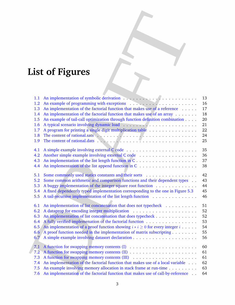
AFTList of Figures

1.1 An implementation of symbolic derivation . . . . . . . . . . . . . . . . . . . . . . . 13

1.2 An example of programming with exceptions . . . . . . . . . . . . . . . . . . . . . 16

1.3 An implementation of the factorial function that makes use of a reference . . . . . 17

1.4 An implementation of the factorial function that makes use of an array . . . . . . . 18

1.5 An example of tail-call optimization through function definition combination . . . . 20

1.6 A typical scenario involving dynamic load . . . . . . . . . . . . . . . . . . . . . . . 21

1.7 A program for printing a single digit multiplication table . . . . . . . . . . . . . . . 22

1.8 The content of rational.sats . . . . . . . . . . . . . . . . . . . . . . . . . . . . . . . 24

1.9 The content of rational.dats . . . . . . . . . . . . . . . . . . . . . . . . . . . . . . . 25

4.1 A simple example involving external C code . . . . . . . . . . . . . . . . . . . . . . 35

4.2 Another simple example involving external C code . . . . . . . . . . . . . . . . . . 36

4.3 An implementation of the list length function in C . . . . . . . . . . . . . . . . . . . 37

4.4 An implementation of the list append function in C . . . . . . . . . . . . . . . . . . 38

5.1 Some commonly used statics constants and their sorts . . . . . . . . . . . . . . . . 42

5.2 Some common arithmetic and comparison functions and their dependent types . . 43

5.3 A buggy implementation of the integer square root function . . . . . . . . . . . . . 44

5.4 A fixed dependently typed implementation corresponding to the one in Figure 5.3 45

5.5 A tail-recursive implementation of the list length function . . . . . . . . . . . . . . 46

6.1 An implementation of list concatenation that does not typecheck . . . . . . . . . . 51

6.2 A dataprop for encoding integer multiplication . . . . . . . . . . . . . . . . . . . . 52

6.3 An implementation of list concatenation that does typecheck . . . . . . . . . . . . . 52

6.4 A fully verified implemenation of the factorial function . . . . . . . . . . . . . . . . 53

6.5 An implementation of a proof function showing i ∗ i ≥ 0 for every integer i . . . . . 54

6.6 A proof function needed in the implementation of matrix subscripting . . . . . . . . 55

6.7 A simple example involving datasort declaration . . . . . . . . . . . . . . . . . . . . 56

7.1 A function for swapping memory contents (I) . . . . . . . . . . . . . . . . . . . . . 60

7.2 A function for swapping memory contents (II) . . . . . . . . . . . . . . . . . . . . . 61

7.3 A function for swapping memory contents (III) . . . . . . . . . . . . . . . . . . . . 61

7.4 An implementation of the factorial function that makes use of a local variable . . . 62

7.5 An example involving memory allocation in stack frame at run-time . . . . . . . . . 63

7.6 An implementation of the factorial function that makes use of call-by-reference . . 64

3

DR

AFT

4 LIST OF FIGURES

7.7 A dataview for modeling arrays . . . . . . . . . . . . . . . . . . . . . . . . . . . . . 64

7.8 Two proof functions for manipulating array views . . . . . . . . . . . . . . . . . . . 66

7.9 Two function templates for reading from and writing to a given array cell . . . . . . 67

7.10 Another proof function for manipulating array views . . . . . . . . . . . . . . . . . 68

7.11 A function template for freeing a given linear list . . . . . . . . . . . . . . . . . . . 69

7.12 A function template for computing the length of a given linear list . . . . . . . . . . 69

DR

AFT

Chapter 1

ATS BASICS

ATS is a rich programming language with a highly expressive type system and a large variety of

programming features. The core of ATS is a call-by-value functional programming language that

is similar to the core of Standard ML (Milner et al., 1997) in terms of both syntax and dynamic

semantics.

This chapter primarily serves as a tutorial introduction to the basics of ATS, and more advanced

and more interesting programming features in ATS will be presented gradually in the following

chapters.

1.1 A Simple Example: Hello, world!

We first use a simple example to explain how programs written in ATS can be compiled and then

executed.

The following program is written in the syntax of ATS, where the function main is a special one.

For those who are familiar with C, this function essentially corresponds to the function in C that is

given the same name.

implement main () = begin

print_string ("Hello, world!"); print_newline ()

end // end of [main]

The keyword implement indicates an implementation of a function that is declared elsewhere.

For instance, the function main is already declared somewhere in ATS as follows:

fun main (): void

which indicates that main is a nullary function that returns no value.

The function print string takes a string as its only argument and prints out the string onto the

standard output while the function print newline takes no argument and prints a newline character

onto the standard output. Also, the keywords begin and end act as a pair of parentheses, and a

line of comment is initiated with two consecutive appearances of the character /.

Now suppose that the above simple program is stored in a file named hello world.dats. Then

the following command, if executed successfully, first generates a file named hello world dats.c

5

DR

AFT

6 CHAPTER 1. ATS BASICS

containing some C code translated from the ATS program in hello world.dats and then invokes gcc

to compile this file into an executable file named hello world:

atscc -o hello_world hello_world.dats

As can be expected, the executable hello world is to print out the message ”Hello, world!” and

a newline character (onto the standard output) when executed.

The command atscc essentially invokes atsopt, an ATS compiler implemented in ATS itself, to

translate ATS programs into C programs and then relies on a C compiler (e.g., gcc) to compile

the generated C programs into machine code. More details on atscc and atsopt will be given in

Chapter 2.

1.2 Elements of Programming

In ATS, there are many forms of expressions as well as means to combining simpler expressions

into compound ones, and we are to introduce these forms and means gradually.

1.2.1 Comments

There are four forms of comments in ATS: line comment, block comment of ML-style, block com-

ment of C-style, and rest-of-file comment.

• A line comment starts with the token // and extends until the end of the current line.

• A block comment of ML-style starts and closes with the tokens (* and *), respectively. Note

that nested block comments of ML-style are allowed, that is, one block comment of ML-style

can occur within another one of the same style.

• A block comment of C-style starts and closes with the tokens /* and */, respectively. Note

that block comments of C-style cannot be nested. The use of block comments of C-style is

primiarily in code that is supposed to be shared by ATS and C. In other cases, block comments

of ML-style should be the preferred choice.

• A rest-of-file comment starts with the token //// (4 consecutive occurrences of /) and ex-

tends until the end of the file.

In the following code (whose meaning is to become clear later), three forms of comments are

present:

fun f91 (x: int): int = // we implement the famous McCarthy’s 91-function

(* this function always return 91 when applied to an integer less than 101 *)

if x < 101 then f91 (f91 (x + 11)) else x - 10

//// whatever written here or below is considered comment

DR

AFT

1.2. ELEMENTS OF PROGRAMMING 7

1.2.2 Primitive Expressions

We informally mention the syntax for some primitive expressions:

• booleans: the truth values are represented as true and false.

• integers: the syntax for integers (in decimal notation) is a sequence of digits that may be

following the negative sign ~ (not the symbol -). For instance, 31415926 and ~27172828 are

integers. Note that the first digit of an integer (in decimal notation) cannot be 0 unless the

integer consists of only a single digit.

The octal digits are from 0 to 7, and an integer in octal notation is a sequence of such digits

following 0.

The hexadecimal digits are the decimal digits extended with letters from a to f, where the

case of such a letter is insensitive. An integer in hexadecimal notation is a sequence of

hexadecimal digits following 0x or 0X.

• float point numbers: the syntax for reals is an integer in decimal notation possibly followed

by a point (.) and one or more decimal digits, possibly followed by an exponent symbol (e or

E) and an integer constant in decimal notation; at least one of the optional parts must occur,

and hence no integer constant is a real constant. Here are some examples of reals: 3.1416,

31416E-4, 271.83e-2, and non-examples of reals: 23, .1, 3.E2, 1.e2.3.

• characters: the syntax for characters is ’c’, where c ranges over ASCII characters, or ’\c’where c ranges over some special characters (e.g., n, t), or ’\ddd’, where d ranges over octal

digits, that is, digits from 0 to 7.

• strings: the syntax for strings is a sequence of characters inside a pair of quotes. For instance,

"Hello, world!\n" is a string, where \n is an escape sequence representing the newline

character.

• special constants:

– An occurrence of the keyword #FILENAME refers to a string that represents the name of

the file in which this occurrence appears.

– An occurrence of the keyword #LOCATION refers to a string that represents the location

of this occurrence.

1.2.3 Fixity

In ATS, prefix, infix and postfix operators are all supported. Given an operator, its fixity status is

either prefix, infix, postfix or none. An operator is said to possess some fixity if its fixity status

is not none. The keywords prefix and postfix are for introducing prefix and postfix operators,

respectively, and the keywords infix, infixl and infixr for introducing non-associative, left-

associative, and right-associated infix operators, respectively. These keywords can be followed by

an optional integer to indicate the precedence of the introduced operators. As an example, the

operator !! is declared to be of the postfix fixity in the following code (whose precise meaning

should become clear later):

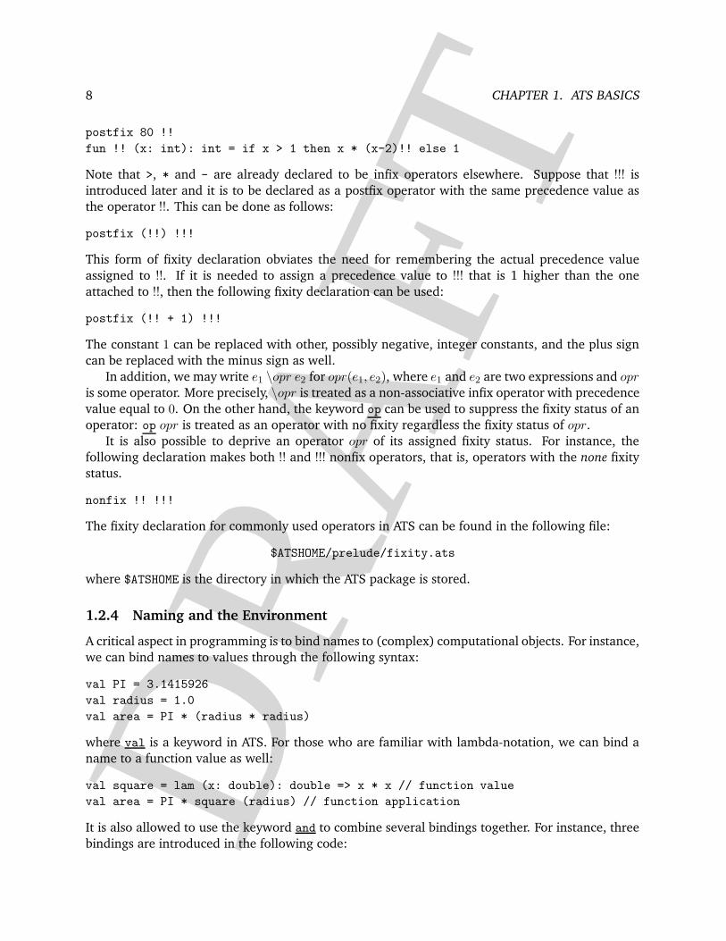
DR

AFT


postfix 80 !!

fun !! (x: int): int = if x > 1 then x * (x-2)!! else 1

Note that >, * and - are already declared to be infix operators elsewhere. Suppose that !!! is

introduced later and it is to be declared as a postfix operator with the same precedence value as

the operator !!. This can be done as follows:

postfix (!!) !!!

This form of fixity declaration obviates the need for remembering the actual precedence value

assigned to !!. If it is needed to assign a precedence value to !!! that is 1 higher than the one

attached to !!, then the following fixity declaration can be used:

postfix (!! + 1) !!!

The constant 1 can be replaced with other, possibly negative, integer constants, and the plus sign

can be replaced with the minus sign as well.

In addition, we may write e1 \opr e2 for opr(e1, e2), where e1 and e2 are two expressions and opris some operator. More precisely, \opr is treated as a non-associative infix operator with precedence

value equal to 0. On the other hand, the keyword op can be used to suppress the fixity status of an

operator: op opr is treated as an operator with no fixity regardless the fixity status of opr.

It is also possible to deprive an operator opr of its assigned fixity status. For instance, the

following declaration makes both !! and !!! nonfix operators, that is, operators with the none fixity

status.

nonfix !! !!!

The fixity declaration for commonly used operators in ATS can be found in the following file:

$ATSHOME/prelude/fixity.ats

where $ATSHOME is the directory in which the ATS package is stored.

1.2.4 Naming and the Environment

A critical aspect in programming is to bind names to (complex) computational objects. For instance,

we can bind names to values through the following syntax:

val PI = 3.1415926

val radius = 1.0

val area = PI * (radius * radius)

where val is a keyword in ATS. For those who are familiar with lambda-notation, we can bind a

name to a function value as well:

val square = lam (x: double): double => x * x // function value

val area = PI * square (radius) // function application

It is also allowed to use the keyword and to combine several bindings together. For instance, three

bindings are introduced in the following code:

DR

AFT

1.2. ELEMENTS OF PROGRAMMING 9

// as the evaluation order is unspecified, it should *not* be expected that

// the printout is "xyz" in this case:

val x = (print_string "x"; 1)

and y = (print_string "y"; 2)

and z = (print_string "z"; 3)

When bindings are combined in this manner, it should be emphasized that the order in which these

binding are evaluated is unspecified.

1.2.5 Conditionals

The syntax for forming a conditional (expression) is given as follows:

if 〈exp〉 then 〈exp〉 else 〈exp〉

where 〈exp〉 ranges over expression in ATS. It is also allowed to form a conditional as follows:

if 〈exp〉 then 〈exp〉

which is simply treated as a shorthand for

if 〈exp〉 then 〈exp〉 else ()

Note that () represents the only value that is of type void . This special value is often referred to as

the void value as its size is 0 (and thus no memory is needed to store it).

1.2.6 Local Bindings

A let-expression is of the following form:

let 〈bindings〉 in 〈scope〉 end

where the (local) bindings placed between the keywords let and in can only be accessed in

the scope of the let-expression. For instance, there are three local bindings in the following let-

expression, which are for x, y and z, respectively:

let

val x = 1; val y = x + x; val z = y * y // the semicolons are optional here

in

x + y + z

end

Another way to introduce local bindings is through the use of a where-clause. For instance, the

above let-expression can be rewritten as follows:

x + y + z where {

val x = 1; val y = x + x; val z = y * y // the semicolons are optional here

} // end of [where]

DR

AFT


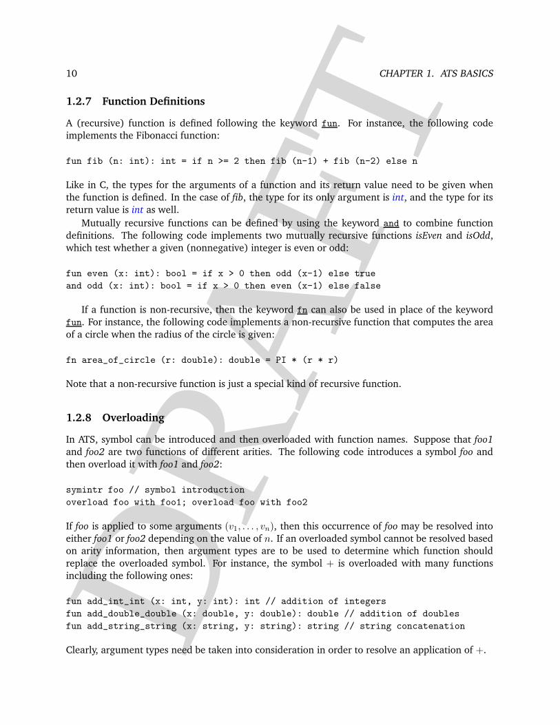
1.2.7 Function Definitions

A (recursive) function is defined following the keyword fun. For instance, the following code

implements the Fibonacci function:

fun fib (n: int): int = if n >= 2 then fib (n-1) + fib (n-2) else n

Like in C, the types for the arguments of a function and its return value need to be given when

the function is defined. In the case of fib, the type for its only argument is int, and the type for its

return value is int as well.

Mutually recursive functions can be defined by using the keyword and to combine function

definitions. The following code implements two mutually recursive functions isEven and isOdd,

which test whether a given (nonnegative) integer is even or odd:

fun even (x: int): bool = if x > 0 then odd (x-1) else true

and odd (x: int): bool = if x > 0 then even (x-1) else false

If a function is non-recursive, then the keyword fn can also be used in place of the keyword

fun. For instance, the following code implements a non-recursive function that computes the area

of a circle when the radius of the circle is given:

fn area_of_circle (r: double): double = PI * (r * r)

Note that a non-recursive function is just a special kind of recursive function.

1.2.8 Overloading

In ATS, symbol can be introduced and then overloaded with function names. Suppose that foo1

and foo2 are two functions of different arities. The following code introduces a symbol foo and

then overload it with foo1 and foo2:

symintr foo // symbol introduction

overload foo with foo1; overload foo with foo2

If foo is applied to some arguments (v1, . . . , vn), then this occurrence of foo may be resolved into

either foo1 or foo2 depending on the value of n. If an overloaded symbol cannot be resolved based

on arity information, then argument types are to be used to determine which function should

replace the overloaded symbol. For instance, the symbol + is overloaded with many functions

including the following ones:

fun add_int_int (x: int, y: int): int // addition of integers

fun add_double_double (x: double, y: double): double // addition of doubles

fun add_string_string (x: string, y: string): string // string concatenation

Clearly, argument types need be taken into consideration in order to resolve an application of +.

DR

AFT

1.3. TUPLES AND RECORDS 11

1.3 Tuples and Records

There are two kinds of tuples in ATS: boxed tuples and flat tuples.

Given values v1, . . . , vn, a tuple ′(v1, . . . , vn) of length n can be formed such that the ith com-

ponent of the tuple is vi for 1 ≤ i ≤ n. The use of the quote symbol ′ is to indicate that this is a

boxed tuple. For instance, a pair boxed 0 1 is formed as follows:

val boxed_1_2 = ’(1, 2)

The components of a tuple can be extracted out by pattern matching. For instance, the following

code binds x and y to 0 and 1, respectively:

val ’(x, y) = boxed_1_2

A tuple of length n is essentially a record with labels ranging from 0 to n − 1. So the components

of a tuple can also be extracted out by field selection:

val x = boxed_1_2.0 and y = boxed_1_2.1

If values v1, . . . , vn are assigned types T1, . . . , Tn, respectively, then the boxed tuple ′(v1, . . . , vn)can be assigned the type ′(T1, . . . , Tn). The size of a boxed tuple is always one word.

A flat tuple is like a struct in C. For instance, a pair flat 0 1 is formed as follows:

val flat_1_2 = @(1, 2) // the @ symbol is optional and may be omitted

Like a boxed tuple, the components of a flat tuple can be extracted out by pattern matching or by

field selection:

val @(x, y) = flat_1_2 // the @ symbol is optional and may be omitted

val x = flat_1_2.0 and y = flat_1_2.1

If values v1, . . . , vn are assigned types T1, . . . , Tn, respectively, then the flat tuple @(v1, . . . , vn) can

be assigned the type @(T1, . . . , Tn). The size of a flat tuple is not specified but it should be greater

than or equal to the sum of the sizes of its components. In other words, we have:

sizeof (@(T1, . . . , Tn)) ≥ sizeof (T1) + . . . + sizeof (Tn)

There are also two kinds of records in ATS: boxed records and flat records. For instance, the

previous boxed tuple example can be done with a record as follows:

val boxed_1_2 = ’{one= 1, two= 2}

val ’{one= x, two= y} = boxed_1_2 // record pattern matching

val ’{one= x, ...} = boxed_1_2 // record pattern matching with omission

val ’{two= y, ...} = boxed_1_2 // record pattern matching with omission

val x = boxed_1_2.one and y = boxed_1_2.two // field selection

The following is an example involving flat records.

DR

AFT


typedef complex = @{real=double, imag=double}

// extracting out record fields by pattern matching

fn magnititute_complex (z: complex): double = let

val @{real= r, imag= i} = z // the @ symbol cannot be omitted

in

sqrt (r * r + i * i)

end

// extracting out record fields by field selection

fn add_complex_complex (z1: complex, z2: complex): complex = begin

@{real= z1.real + z2.real, imag= z1.imag + z2.imag}

end

1.4 Disjoint Variants

Like in ML, A disjoint variant type is often referred to as a datatype in ATS. For instance, we can

declare a datatype weekday as follows:

datatype weekday = Monday | Tuesday | Wednesday | Thursday | Friday

There are five data constructors Monday, Tuesday Wednesday, Thursday and Friday associated with

the datatype weekday. In this case, all the data constructors are nullary, that is, they take no

arguments to form data. Note that there are no restrictions on the names of data constructors in

ATS: any valid identifiers can be used.

The datatype weekday is rather close to an enumerate type in C. In the following code, a func-

tion is implemented that translates values of the type weekday into integers:

fn int_of_weekday (x: weekday): int = case+ x of

| Monday () => 1

| Tuesday () => 2

| Wednesday () => 3

| Thursday () => 4

| Friday () => 5

Given a nullary data constructor C, it is important to write C() (instead of just C) in order to form

a pattern. If C is used as a pattern, then it is a variable pattern that matches any value. If Monday

(instead of Monday()) is used in the implementation of int of weekday , then the ATS typechecker

will issue an error message stating that all the pattern matching clauses following the first one are

redundant as the variable pattern Monday already matches all the possible values that x may take.

If a case-expression is formed with the keyword case+, then the ATS typechecker needs to verify

that the pattern matching for this case-expression is exhaustive. For instance, if the last pattern

matching clause in the implementation of int of weekday is dropped, then the ATS typechecker

will issue an error stating that the involved pattern matching is not exhaustive. If the keyword

case is used in place of case+, then the typechecker will only issue a warning message. If the

keyword case- is used instead, then the compiler will issue no message.

As another example, a datatype involving non-nullary data constructors is given as follows:

DR

AFT

1.5. PARAMETRIC POLYMORPHISM AND TEMPLATES 13

datatype exp =

| EXPcst of double | EXPvar of string

| EXPadd of (exp, exp) | EXPsub of (exp, exp)

| EXPmul of (exp, exp) | EXPdiv of (exp, exp)

| EXPpow of (exp, int)

The declared datatype exp is for values representing expressions formed in terms of constants and

variables as well as addition, subtraction, multiplication, division, and the exponential function

where the exponent is restricted to being a integer constant. In Figure 1.1, a function named

val expcst_0 = EXPcst 0.0 and expcst_1 = EXPcst 1.0

fn exp_derivate (e0: exp, x0: string): exp = let

fun aux (e0: exp):<cloref1> exp = case+ e0 of

| EXPcst _ => expcst_0

| EXPvar x => if (x = x0) then expcst_1 else expcst_0

| EXPadd (e1, e2) => EXPadd (aux e1, aux e2)

| EXPsub (e1, e2) => EXPsub (aux e1, aux e2)

| EXPmul (e1, e2) => begin

EXPadd (EXPmul (aux e1, e2), EXPmul (e1, aux e2))

end

| EXPdiv (e1, e2) => begin EXPdiv

(EXPsub (EXPmul (aux e1, e2), EXPmul (e1, aux e2)), EXPpow (e2, 2))

end

| EXPpow (e, n) => begin

EXPmul (EXPcst (double_of_int n), EXPmul (EXPpow (e, n-1), aux e))

end

// end of [aux]

in

aux (e0)

end // end of [exp_derivate]

Figure 1.1: An implementation of symbolic derivation

exp derivate is implemented to perform symbolic derivation on expressions thus formed.

1.5 Parametric Polymorphism and Templates

Parametric polymorphism (or polymorphism for short) offers a flexible and effective approach to

supporting code reuse. For instance, given a pair (v1, v2) where v1 is a a boolean and v2 a character,

the function swap bool char defined below returns a pair (v2, v1):

fun swap_bool_char (xy: @(bool, char)): @(char, bool) = (xy.1, xy.0)

Now suppose that a pair of integers need to be swapped, and this results in the implementation of

the following function swap int int:

DR

AFT


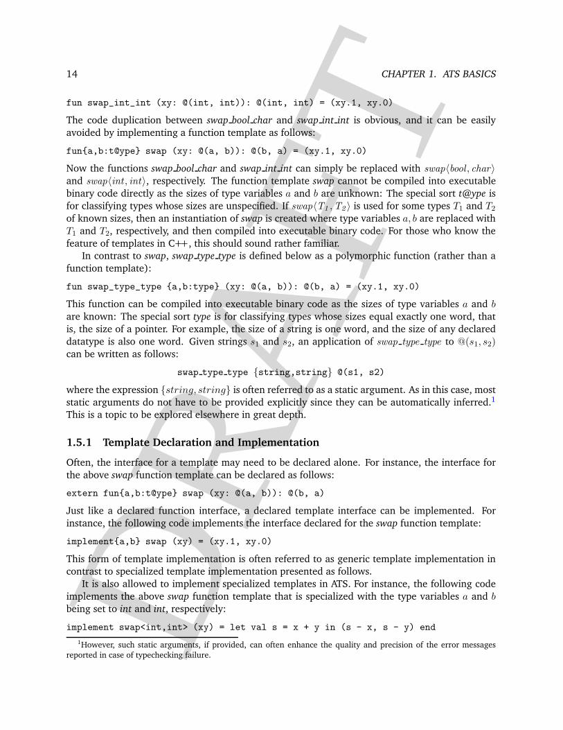
fun swap_int_int (xy: @(int, int)): @(int, int) = (xy.1, xy.0)

The code duplication between swap bool char and swap int int is obvious, and it can be easily

avoided by implementing a function template as follows:

fun{a,b:t@ype} swap (xy: @(a, b)): @(b, a) = (xy.1, xy.0)

Now the functions swap bool char and swap int int can simply be replaced with swap〈bool , char〉and swap〈int , int〉, respectively. The function template swap cannot be compiled into executable

binary code directly as the sizes of type variables a and b are unknown: The special sort t@ype is

for classifying types whose sizes are unspecified. If swap〈T1 ,T2 〉 is used for some types T1 and T2

of known sizes, then an instantiation of swap is created where type variables a, b are replaced with

T1 and T2, respectively, and then compiled into executable binary code. For those who know the

feature of templates in C++, this should sound rather familiar.

In contrast to swap, swap type type is defined below as a polymorphic function (rather than a

function template):

fun swap_type_type {a,b:type} (xy: @(a, b)): @(b, a) = (xy.1, xy.0)

This function can be compiled into executable binary code as the sizes of type variables a and bare known: The special sort type is for classifying types whose sizes equal exactly one word, that

is, the size of a pointer. For example, the size of a string is one word, and the size of any declared

datatype is also one word. Given strings s1 and s2, an application of swap type type to @(s1, s2)can be written as follows:

swap type type {string,string} @(s1, s2)

where the expression {string, string} is often referred to as a static argument. As in this case, most

static arguments do not have to be provided explicitly since they can be automatically inferred.1

This is a topic to be explored elsewhere in great depth.

1.5.1 Template Declaration and Implementation

Often, the interface for a template may need to be declared alone. For instance, the interface for

the above swap function template can be declared as follows:

extern fun{a,b:t@ype} swap (xy: @(a, b)): @(b, a)

Just like a declared function interface, a declared template interface can be implemented. For

instance, the following code implements the interface declared for the swap function template:

implement{a,b} swap (xy) = (xy.1, xy.0)

This form of template implementation is often referred to as generic template implementation in

contrast to specialized template implementation presented as follows.

It is also allowed to implement specialized templates in ATS. For instance, the following code

implements the above swap function template that is specialized with the type variables a and bbeing set to int and int, respectively:

implement swap<int,int> (xy) = let val s = x + y in (s - x, s - y) end

1However, such static arguments, if provided, can often enhance the quality and precision of the error messages

reported in case of typechecking failure.

DR

AFT

1.6. LISTS 15

1.6 Lists

In ATS, list0 is a type constructor defined as follows:

datatype list0 (a:t@ype) = list0_cons (a) of (a, list0 a) | list0_nil (a)

Given a type T , list0 (T ) is the type for lists consisting of elements of type T :

• list0 nil () forms an empty list.

• Given values v and vs of types T and list0 (T ), respectively, list0 cons(v, vs) forms a list

whose head and tail are v and vs, respectively.

For instance, a list consisting of 1, 2 and 3 can be constructed as follows:

val lst123 = list0_cons (1, list0_cons (2, list0_cons (3, list0_nil ())))

Another notation for constructing lists consisting of elements of type T is

list0 make arrsz $arrszT (v1, . . . , vn)

For instance, a string list consisting names of weekdays is given as follows:

val weekdays (* : list0 string *) = list0_make_arrsz (

$arrsz{string}("Monday", "Tuesday", "Wednesday", "Thursday", "Friday")

) // end of [val]

List manipulation can be done by pattern matching. As an example, the following code implements

a function template for appending two given list arguments:

fun{a:t@ype} list0_append (xs: list0 a, ys: list0 a): list0 a =

case+ xs of

| list0_cons (x, xs) => list0_cons (x, list0_append (xs, ys))

| list0_nil () => ys

Note that this is functional appending: the two given lists are not altered by list0 append.

In ATS, there is also a dependent type constructor list for forming types for lists. As this type

constructor involves more advanced type theory, it is to be presented elsewhere.

1.7 Exceptions

The exception mechanism in ATS is rather similar to the one supported in ML (Milner et al., 1997),

which provides a highly flexible means for the programmer to alter the control flow in program

execution. For instance, an exception (or more precisely, an exception constructor) Fatal is defined

as follows and then used in the implementation of a function.

exception Fatal

fun fatal {a:t@ype} (msg: String): a = (prerr_string msg; $raise Fatal ())

DR

AFT


datatype tree = E | B of (tree, int, tree) // for integer binary trees

fn isPerfect (t: tree): bool = let

exception NotPerfect

fun aux (t: tree): int = case+ t of

| B (t1, _, t2) => let

val h1 = aux (t1) and h2 = aux (t2)

in

if h1 = h2 then h1 + 1 else $raise NotPerfect ()

end

| E () => 0

in

try let val _ = aux (t) in true end with ~NotPerfect () => false

end // end of [isPerfect]

Figure 1.2: An example of programming with exceptions

A call to the defined function fatal with a string argument msg prints msg onto stderr and then

raises the exception Fatal (). Note that a raised exception may be assigned any type.

A raised exception can be trapped. In Figure 1.2, an interesting example of programming with

exceptions is presented. First, a datatype constructor tree is delcared for representing binary trees

(storing integers). Then a function isPerfect is implemented to test whether a given binary tree

is perfectly balanced. The inner function aux computes the height of a given binary tree t if t is

perfectly balanced. Otherwise, aux raises the exception NotPerfect.

Note that the exception NotPerfect is not declared at the top level. Instead, it is declared inside

a let-expression in the body of the function isPerfect and thus is only available in the scope of the

let-expression.

Also note the symbol ˜ in front of an occurrence of NotPerfect in the code. This symbol means

that the captured exception is to be destroyed (as it is no longer needed). If a captured exception

is not destroyed, then it must be used in some way (e.g., to be raised again).

1.8 References

In ATS, a reference is similar to a pointer in C. However, the issue of dangling pointers does not

appear with references as every reference is properly initialized after its creation. Given a type T ,

ref (T ) is the type for references to values of type T . For instance, the following code creates an

integer reference, initializes it with 1 and binds r to it:

val r = ref<int> (1)

The operator ! is specially reserved for dereferencing. For instance, after the expression !r := !r+1is evaluated, the value stored in the memory location referred to by r is increased by 1. Note that

the occurrence of !r to the left of := is a left-value that can be assigned to. In contrast, this

expression would be written as r := !r + 1 in ML.

DR

AFT

1.9. ARRAYS 17

fun fact (x: int): int = let

val res = ref<int> (1)

fun loop (x: int):<cloref1> void =

if x > 0 then (!res := !res * x; loop (x-1))

in

loop (x); !res

end // end of [fact]

Figure 1.3: An implementation of the factorial function that makes use of a reference

As an example, the code in Figure 1.3 is an implementation of the factorial function in ATS that

makes use of a reference. In it, the special syntax :<cloref1> (where no space is allowed between

: and <) is needed to indicate that loop is a closure rather than a function. The difference between

functions and closures will be explained elsewhere in details.

1.9 Arrays

In ATS, array0 is a type constructor for forming array types. Given a type T , the type array0 (T )is for arrays containing elements of type T . Given values v1, . . . , vn of type T , the notation

array0 @[T ][v1, . . . , vn] creates an array of size n that is initialized with the values v1, . . . , vn. The

valid subscripts for an array of size n range from 0 until n− 1. For instance, a string array of size 5is created as follows:

val weekdays = array0 $arrsz{string}(

"Monday", "Tuesday", "Wednesday", "Thursday", "Friday"

) // a string array containing names of weekdays

Array subscripting in ATS is conventional. For instance, weekdays [3] returns the string ”Thursday”,

and the following assignment

weekdays[0] := ”foo”

replaces the content of the first cell of weekdays with the string ”foo”. For arrays of type array0 (T )for some T , array bounds checking is performed at run-time to guarantee safe subscripting.

Given an array A of type array0 (T ), the size of A can be obtained by evaluating the function

call array0 size (A). As an example, the code in Figure 1.4 gives another implementation of the

factorial function. Note that give an integer sz and a value v of some type T , the function call

array0 make elt〈T 〉(sz, v) creates an array of size sz and then initializes all array cells with the

value v.

1.10 Higher-Order Functions

A higher-order function is one that takes a function as its argument. In the following code, the

function derivate is a higher-order function that takes as its argument a closure representing a

function from double to double and returns a closure representing the derivative of the function.

DR

AFT


fn fact (x: int): int = let

// creating an array of size [x] and initialing it with 0’s

val A = array0_make_elt<int> (x, 0)

val () = init (0) where { // initializing [A] with 1, ..., n

fun init (i: int):<cloref1> void =

if i < x then (A[i] := i + 1; init (i + 1)) else ()

} // end of [where]

fun loop (i: int, res: int):<cloref1> int =

if i < x then loop (i+1, res * A[i]) else res

in

loop (0(*i*), 1(*res*))


Figure 1.4: An implementation of the factorial function that makes use of an array

val epsilon = 1E-6

// [double -<cloref1> double] is the type for closures representing

// functions from double to double

fn derivate (f: double -<cloref1> double): double -<cloref1> double =

lam x => (f (x+epsilon) - f (x)) / epsilon

Some code that makes use of the higher-order function derivate is given as follows:

val sin_deriv = derivate (lam x => sin x)

val PI = 4 * (atan 1.0); val theta = PI / 3

val one = // [one] approximately equals 1.0

square (sin theta) + square (sin_deriv theta)

Many list-processing functions are higher-order. As an example, the following code implements a

function template list0 map:

fun{a,b:t@ype} list0_map

(xs: list0 a, f: a -<cloref1> b): list0 b = case+ xs of

| list0_cons (x, xs) => list0_cons (f x, list0_map (xs, f))

| list0_nil () => list0_nil ()

Given a list vs consisting of elements v1, . . . , vn of type T1 and a function f from T1 to T2, the

following call:

list0 map〈T1, T2〉(vs, f)

returns a list consisting of elements f(v1), . . . , f(vn) that are of type T2.

1.11 Tail-Call Optimization

It can probably be argued that the single most important optimization performed by the ATS com-

piler (Anairiats) is the translation of tail-calls into direct (local) jumps.

DR

AFT

1.11. TAIL-CALL OPTIMIZATION 19

As an example, the following defined function sum1 sums up integers from 1 to n when applied

to a given integer n:

// [sum1] is recursive but not tail-recursive

fun sum1 (n: int): int = if n > 0 then n + sum1 (n-1) else 0

This function is recursive but not tail-recursive. The stack space it consumes is proportional to the

value of its argument. Essentially, Anairiats translates the definition of sum1 into the following C

code:

int sum1 (int n) {

if (n > 1) return n + sum1 (n-1) ; else return 1 ;

}

On the other hand, the following defined function sum2 also sums up integers from 1 to n when

applied to a given integer n:

fn sum2 (n: int): int = let // sum2 is non-recursive

fun loop (n: int, res: int): int = // [loop] is tail-recursive

if n > 0 then loop (n-1, res+n) else res

in

loop (n, 0)

end // end of [sum2]

The inner function loop in the definition of sum2 is tail-recursive. The stack space consumed by

loop is a constant independent of th value of the argument of sum2. Essentially, Anairiats translates

the definition of sum2 into the following C code:

int sum2_loop (int n, int res) {

loop: if (n > 0) { res = res + n ; n = n - 1 ; goto loop ; }

return res ;

} /* end of sum2_loop */

int sum2 (int n) { return sum2_loop (n, 0) ; }

Sometimes, function definitions need to be combined in order to identify tail-calls, and the

keyword fn* is reserved for this purpose. In the following example, the keyword fn* indicates to

Anairiats that the function definitions of even and odd need to be combined together so as to turn

(mutually) recursive function calls into direct jumps.

fn* even (n: int): bool = if n > 0 then odd (n-1) else true

and odd (n: int): bool = if n > 0 then even (n-1) else false

Essentially, Anairiats emits the C code in Figure 1.5 after compiling this example. Note that mu-

tually recursive functions can be combined in such a manner only if they all have the same return

type. In the above case, both even and odd have the same return type bool.

DR

AFT


bool even_odd (int tag, int n) {

bool res ; // [bool] is [int]

switch (tag) { 0: goto even ; 1: goto odd ; default : exit (1) ; }

even:

if (n > 0) { n = n - 1; goto odd; } else { res = true; goto done; }

odd:

if (n > 0) { n = n - 1; goto even; } else { res = false; goto done; }

done: return res ;

} /* end of [even_odd] */

bool even (int n) {

return even_odd (0, n) ;

}

bool odd (int n) {

return even_odd (1, n) ;

}

Figure 1.5: An example of tail-call optimization through function definition combination

1.12 Static and Dynamic Files

In ATS, the filename extensions ”.sats” and ”.dats” are used to indicate static and dynamic files,

respectively. These two extensions have some special meaning attached to them and thus cannot

be replaced arbitrarily.

A static file may contain sort definitions, datasort declarations, static definitions, abstract type

declarations, exception declarations, datatype declarations, macro definitions, interfaces for dy-

namic values and functions, etc. These concepts are to be made clear later. In terms of function-

ality, a static file in ATS is similar to a header file (with the filename extension ”.h”) in C or an

interface file (with the filename extension ”.mli”) in Objective Caml.

A dynamic file may contain everything in a static file. In addition, it may also contain definitions

for dynamic values and functions.

In general, the syntax for constructing code in a static file can also be used for constructing

code in a dynamic file. The only exception involves declaring interfaces for dynamic values and

functions. For instance, in a static file, the following syntax can be used to declare interfaces (or

types) for a value named PI and a function named area of circle:

val PI : double

fun area_of_circle (radius: double): double

When the same thing is done in a dynamic file, the keyword extern needs to be put in front of the

declarations:

extern val PI : double

DR

AFT

1.13. STATIC LOAD AND DYNAMIC LOAD 21

extern fun area_of_circle (radius: double): double

As a convention, we often use the filename extension ”.cats” for a file containing some C code

that is supposed to be combined with ATS code in certain manner. However, the use of this filename

extension is not mandatory.

1.13 Static Load and Dynamic Load

The phrase static load refers to either a static or a dynamic file being loaded at compile-time.

Suppose that foo.sats is a static file in which a symbol bar is declared. This symbol may refer to

some value, function, type (constructor), data constructor, etc. In order to access bar (in another

file), one can load foo.sats statically as follows:

staload F = "foo.sats" // [F] can be replaced with any valid name

Then the qualified symbol $F.bar can be used to refer to the declared symbol bar in foo.sats. It is

also possible to load foo.sats statically as follows:

staload "foo.sats" // foo.sats is loaded and then opened

If done in this manner, it suffices to simply write bar to refer to the declared symbol bar in foo.sats.

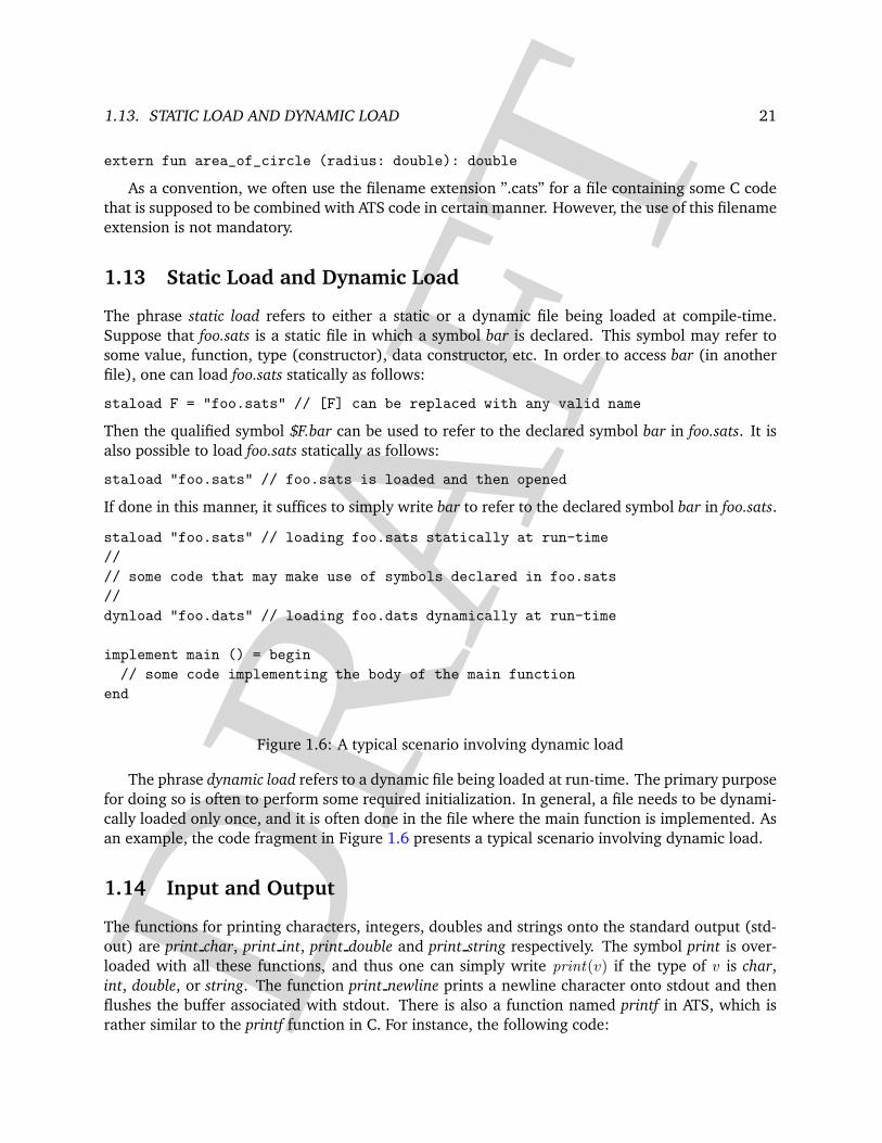
staload "foo.sats" // loading foo.sats statically at run-time

//

// some code that may make use of symbols declared in foo.sats

//

dynload "foo.dats" // loading foo.dats dynamically at run-time


// some code implementing the body of the main function

end

Figure 1.6: A typical scenario involving dynamic load

The phrase dynamic load refers to a dynamic file being loaded at run-time. The primary purpose

for doing so is often to perform some required initialization. In general, a file needs to be dynami-

cally loaded only once, and it is often done in the file where the main function is implemented. As

an example, the code fragment in Figure 1.6 presents a typical scenario involving dynamic load.

1.14 Input and Output

The functions for printing characters, integers, doubles and strings onto the standard output (std-

out) are print char, print int, print double and print string respectively. The symbol print is over-

loaded with all these functions, and thus one can simply write print(v) if the type of v is char,

int, double, or string. The function print newline prints a newline character onto stdout and then

flushes the buffer associated with stdout. There is also a function named printf in ATS, which is

rather similar to the printf function in C. For instance, the following code:

DR

AFT


val () = printf

("c = %c and f = %f and i = %i and s = %s\n", @(’a’, 3.14, 2008, "July")

prints onto stdout the line below:

c = a and f = 3.14 and i = 2008 and s = July

Note that the arguments of printf except the first one, which represents a format string, need to be

grouped together inside @(. . .), where no space is allowed between @ and (.

For all of these functions printing onto stdout, there are corresponding ones that print onto

stderr: prerr char, prerr double, prerr int, prerr string, prerr newline and prerrf.

staload "prelude/SATS/file.sats" // it is loaded so that

// the functions [open_file] and [close_file] become available

#define MAXDIGIT 9 // [MAXDIGIT] is to be replaced with [9]

fun loop_one (fil: FILEref, row: int, col: int): void =

if col <= row then let

val () = if col > 1 then fprint_string (fil, " | ")

val () = fprintf (fil, "%i*%i=%2.2i", @(col, row, col * row))

in

loop_one (fil, row, col + 1)

end else begin

fprint_newline (fil)

end // end of [if]

fun loop_all (fil: FILEref, row: int): void =

if row <= MAXDIGIT then begin

loop_one (fil, row, 1); loop_all (fil, row + 1)

end // end of [if]

implement main () = let

val () = print_string ("Please input a name for the ouput file: ")

val name = input_line (stdin_ref)

val is_stdout = string0_is_empty name

val fil = if is_stdout then stdout_ref else open_file (name, file_mode_w)

val () = loop_all (fil, 1)

val () = if is_stdout then exit (0) else close_file (fil)

in

printf ("The multiplication table is now stored in the file [%s].", @(name));

print_newline ()


Figure 1.7: A program for printing a single digit multiplication table

DR

AFT

1.15. A SIMPLE PACKAGE FOR RATIONAL NUMBERS 23

For handling files, ATS provides a type FILEref that roughly corresponds to the type FILE* in

C. There are three special values stdin ref, stdout ref and stderr ref of type FILEref in ATS, which

correspond to stdin, stdout and stderr in C, respectively. A variety of file operations are declared in

the following file:

$ATSHOME/libc/SATS/stdio.sats

which all have counterparts in C.

In Figure 1.7, a complete ATS program is constructed to produce the following table for single

digit multiplication:

1*1=01

1*2=02 | 2*2=04

1*3=03 | 2*3=06 | 3*3=09

1*4=04 | 2*4=08 | 3*4=12 | 4*4=16

1*5=05 | 2*5=10 | 3*5=15 | 4*5=20 | 5*5=25

1*6=06 | 2*6=12 | 3*6=18 | 4*6=24 | 5*6=30 | 6*6=36

1*7=07 | 2*7=14 | 3*7=21 | 4*7=28 | 5*7=35 | 6*7=42 | 7*7=49

1*8=08 | 2*8=16 | 3*8=24 | 4*8=32 | 5*8=40 | 6*8=48 | 7*8=56 | 8*8=64

1*9=09 | 2*9=18 | 3*9=27 | 4*9=36 | 5*9=45 | 6*9=54 | 7*9=63 | 8*9=72 | 9*9=81

The following explanation is for several functions in this program that deal with I/O:

• open file creates a file handle, i.e., a value of type FILEref when applied to a string (represent-

ing the path to the file to be created) and a file mode.

• close file closes a given file handle.

• input line reads a line from a given file handle and then returns a string representing the line

minus the last newline character. In case the end of file is reached before a newline character

is encountered, input line returns a string consisting of all the characters read.

1.15 A Simple Package for Rational Numbers

We implement a simple package for rational numbers in this section. This implementation consists

of two files named rational.sats and rational.dats.

The content of rational.sats is given in Figure 1.8. First, an abstract type rat is introduced. The

sort of rat is type, which indicates that the size of rat is one word. Next, an exception constructor is

declared for forming exceptions to be raised in case of a division-by-zero error. In addition, some

functions for creating and handling rational numbers are declared.

In Figure 1.9, the content of rational.dats is shown. First, the file rational.sats is loaded stati-

cally. Next, the abstract type rat is assumed to be a boxed record type with fields numer and denom.

This assumption is available to the rest of the file (but not outside the file), and it is needed for

verifying that the implementation of each function declared in rational.sats is well-typed.

DR

AFT


abstype rat // a boxed abstract type for rational numbers

exception DenominatorIsZeroException // an exception constructor

// rat_make_int (p) = p / 1

fun rat_make_int (numer: int): rat

// rat_make_int_int (p, q) = p / q

fun rat_make_int_int (numer: int, denom: int): rat

symintr rat_make // [rat_make] is introduced for overloading

overload rat_make with rat_make_int

overload rat_make with rat_make_int_int

fun add_rat_rat (r1: rat, r2: rat): rat and sub_rat_rat (r1: rat, r2: rat): rat

fun mul_rat_rat (r1: rat, r2: rat): rat and div_rat_rat (r1: rat, r2: rat): rat

overload + with add_rat_rat; overload - with sub_rat_rat

overload * with mul_rat_rat; overload / with div_rat_rat

fun fprint_rat (out: FILEref, r: rat): void

// the symbol [fprint] is already introduced elsewhere

overload fprint with fprint_rat

Figure 1.8: The content of rational.sats

DR

AFT

1.15. A SIMPLE PACKAGE FOR RATIONAL NUMBERS 25

staload "rational.sats"

assume rat = ’{numer= int, denom= int} // a boxed record

implement rat_make_int (p) = ’{numer= p, denom= 1}

fn rat_make_int_int_main (p: int, q: int): rat = let

val g = gcd (p, q) in ’{numer= p / g, denom= q / g}

end // end of [rat_make_int_int_main]

implement rat_make_int_int (p, q) = case+ 0 of

| _ when q > 0 => rat_make_int_int_main (p, q)

| _ when q < 0 => rat_make_int_int_main (~p, ~q)

| _ (*q=0*) => $raise DenominatorIsZeroException ()

implement add_rat_rat (r1, r2) =

rat_make_int_int_main (p1 * q2 + p2 * q1, q1 * q2) where {

val ’{numer=p1, denom=q1} = r1 and ’{numer=p2, denom=q2} = r2

} // end of [add_rat_rat]

implement sub_rat_rat (r1, r2) =

rat_make_int_int_main (p1 * q2 - p2 * q1, q1 * q2) where {


} // end of [sub_rat_rat]

implement mul_rat_rat (r1, r2) =

rat_make_int_int_main (p1 * p2, q1 * q2) where {


} // end of [mul_rat_rat]

implement div_rat_rat (r1, r2) =

rat_make_int_int (p1 * q2, p2 * q1) where {


} // end of [div_rat_rat]

implement fprint_rat (out, r) =

let val p = r.numer and q = r.denom in

if q = 1 then fprint_int (out, p) else begin

fprint_int (out, p); fprint_char (out, ’/’); fprint_int (out, q)

end // end of [if]

end // end of [fprint_rat]

Figure 1.9: The content of rational.dats

DR

AFT


DR

AFT

Chapter 2

BATCH COMPILATION

The command for compiling ATS programs into C code is atsopt. After C code is emitted by atsopt,

it can then be compiled into machine code by gcc. The command atscc, which essentially combines

atsopt and gcc, compiles ATS programs directly into machine code. Both atsopt and atscc are

implemented in ATS. If a C compiler other than gcc is to be used, the command name for this C

compiler needs to be defined in the environment variable ATSCCOMP.

2.1 The Command atsopt

The command atsopt compiles ATS programs into C code. This command is primarily used in

scripting files such as those needed by the make command.

2.1.1 Compiling Static and Dynamic Files

The following command line compiles a dynamic file foo.dats into C code:

atsopt -d foo.dats

and the output is directed to stdout. The flag -d may be replaced with ‘–dynamic‘.

Suppose it is desired to store the emitted C code into a file with the name foo dats.c, the

following command line can be issued:

atsopt -o foo_dats.c -d foo.dats

The flag -o may also be replaced with ‘–output‘. It should be emphasized that the part -o foo_dats.c

must be put in front of -d foo.dats.

Similarly, the following command line compiles a static file foo.sats into C code:

atsopt -s foo.sats

and the output is directed to stdout. The flag -s may be replaced with ‘–static‘. If the follow-

ing command line is issued (and executed successfully), then the C code emitted from compiling

foo.sats and foo.dats is to be stored in files foo sats.c and foo dats.c, respectively.

atsopt -o foo_sats.c -s foo.sats -o foo_dats.c -d foo.dats

27

DR

AFT

28 CHAPTER 2. BATCH COMPILATION

2.1.2 Typechecking Only

If the following command line is issued, then the file foo.dats is only typechecked:

atsopt -tc -d foo.dats

The flag -tc may be replaced with ‘–typecheck‘. Even if the file foo.dats passes typechecking, no

efffort is to be made to emit C code from compiling foo.dats. If both foo.dats and foo.sats need to

be typechecked, it can be done as follows:

atsopt -tc -d foo.dats -s foo.sats

2.1.3 Generating HTML Files

The flag --posmark_html can be used to turn ATS programs into HTML files for the purpose

of viewing (through a browser). For instance, if the following command line is issued, a file

foo dats.html is generated:

atsopt --posmark_html -d foo.dats > foo_dats.html

2.1.4 Generating HTML Files for cross-referencing

The flag --posmark_xref can be used to turn ATS programs into HTML files for the purpose of

viewing and cross-referencing (through a browser). For instance, if the following command line is

issued, a file foo dats.html is generated while various other files are created in the directory XREF/

for the purpose of cross-referencing:

atsopt --posmark_xref=XREF -d foo.dats > foo_dats.html

2.1.5 Generating Usage Information

The following command line can be issued to generate some brief information on the usage of

atsopt:

atsopt -h

The flag -h may be replaced with ‘–help‘.

2.1.6 Generating Version Information

The following command line can be issued to generate version information on atsopt:

atsopt -v

The flag -v may be replaced with ‘–version‘.

2.2 The Command atscc

The command atscc combines atsopt and gcc, and it is designed to be used in both command lines

and scripting files. Explanation on special flags for atscc is given as follows. If a flag is not special

to atscc, it is passed to gcc directly by atscc.

DR

AFT

2.2. THE COMMAND ATSCC 29

2.2.1 Generating Executables

The following command line, if executed successfully, generates an executable file a.out:

atscc foo.dats foo.sats

Essentially, this command line is equivalent to the following one:

atsopt -o foo_dats.c -d foo.dats -o foo_sats.c -s foo.sats ; \

gcc -I $ATSHOME -I $ATSHOME/ccomp/runtime -L $ATSHOME/ccomp/lib foo_dats.c -lats

If the generated executable needs to be given the name foo, then the following command line

can be issued:

atscc -o foo foo.dats foo.sats

Of course, flags for gcc such as -O2, -Wall and -fomit-frame-pointer can be added freely as is

done in the following command line:

atscc -O2 -o foo -Wall -fomit-frame-pointer foo.dats foo.sats

2.2.2 Typechecking Only

The flag -tc or --typecheck is used to indicate typechecking only. For instance, the following

command line:

atscc -tc foo.sats foo.dats

is equivalent to the one below:

atsopt -tc --static foo.sats --dynamic foo.dats

2.2.3 Compilation Only

The flag -cc or --compile is used to indicate compilation only. For instance, the following com-

mand line:

atscc -cc foo.sats foo.dats

is equivalent to the one below:

atsopt -o foo_sats.c --static foo.sats -o foo_dats.c --dynamic foo.dats

2.2.4 Binary Types

The flags -m32 and -m64 can be passed to indicate the need for generating binaries running on

32-bit and 64-bit machines, respectively.

DR

AFT

30 CHAPTER 2. BATCH COMPILATION

2.2.5 Garbage Collection

By default, executables generated by atscc run without garbage collection (GC). If executables need

to be generated that run with GC being turned on, the flag -D_ATS_GCATS should be present. For

instance, the follow command line generates such an executable named foo:

atscc -D_ATS_GCATS -o foo foo.dats foo.sats

Note that the flag -D_ATS_GCATS should only be used when atscc is called to generate executables.

2.2.6 Directories for File Search

The use of -IATS by atscc is analogous to -I by gcc. By default, atscc searches for files only in the

directory $ATSHOME and the current directory. If more directories need to be searched, it can be

added as follows:

atscc -IATS barpath1 -IATS barpath2 foo.sats foo.dats

where barpath1 and barpath2 represent paths to some existing directories. The space following

-IATS is optional and it can be erased if desired. Note that this command-line feature also applies

to the command atsopt.

2.2.7 Setting Command-Line Flags

The use of -DATS by atscc is analogous to -D by gcc. For instance, the following command-line:

atscc -DATS FOO=123 -DATS BAR=xyz foo.sats foo.dats

first sets FOO and BAR to strings ”123” (instead of the integer 123) and ”xyz”, respectively, and

then compiles the files foo.sats and foo.dats. The space following -DATS is optional and it can be

erased if desired. Note that this command-line feature also applies to the command atsopt.

DR

AFT

Chapter 3

Macros

There are two kinds of macros in ATS. One kind is C-like and the other one is LISP-like, though

they are much simpler as well as weaker than their counterparts in C and LISP, respectively.

3.1 C-like Macros

We use some examples to illustrate certain typical uses of C-like macros in ATS.

The following two declarations bind the identifiers N1 and N2 to the abstract syntax trees (rather

than strings) that represent 1024 and N1 + N1, respectively:

#define N1 1024; #define N2 N1 + N1

Suppose we have the following value declaration appearing in the scope of the above macro

delarations:

val x = N1 * N2

Then N1∗N2 first expands into 1024∗(N1+N1), which further expands into 1024∗(1024+1024).Note that if this example is done in C, then N1∗N2 expands into 1024∗1024+1024, which is different

from what we have in ATS. Also note that it makes no diffierence if we reverse the order of the

previous macro definitions:

#define N2 N1 + N1; #define N1 1024

If we declare a marco as follows:

#define LOOP (LOOP + 1)

then an infinite loop is entered (or more precisely, some macro expansion depth is to be reached)

when the identifier LOOP is expanded.

3.2 LISP-like Macros

There are two forms of LISP-like macros in ATS: short form and long form. These (untyped)

macros are highly flexible and expressive, and they can certainly be used in convoluted manners

that should probably be avoided in the first place. Some commonly used macro definitions can be

found in the following file:

31

DR

AFT

32 CHAPTER 3. MACROS

$ATSHOME/prelude/macrodef.sats

In order to use LISP-like macros in ATS effectively, the programmer may want to find some exam-

ples in LISP involving backquote-comma-notation.

3.2.1 Macros in Long Form

As a macro in short form can simply be considered a special kind of macro in long form, we first

give some explanantion on the latter. A macro definition in long form is introduced via the use of

the keyword macrodef. For instance, the following syntax introduces a macro name one that refers

to some code, that is, abstract syntax tree (AST) representing the integer number 1.

macrodef one = ‘(1)

The special syntax ‘(...), where no space is allowed between the backquote symbol and the

left parenthsis symbol, means to form an abstract syntax tree representing what is written inside

the parentheses. This is often referred to as backquote-notation. Intuitively, one may think that a

backquote-notation exerts an effect that freezes everything inside it.

Let us now define another macro as follows:

macrodef one_plus_one = ‘(1 + 1)

The defined macro name one plus one refers to some code (i.e., AST) representing 1 + 1. At this

point, it is important to stress that the code representing 1+1 is different from the code representing

¡i¿2¡/i¿. The macro name one plus one can also be defined as follows:

macrodef one_plus_one = ‘(,(one) + ,(one))

The syntax ,(...), where no space is allowed between the comma symbol and the left paren-

thesis symbol, indicates the need to expand (or evaluate) whatever is written inside the paren-

theses. This is often referred to as comma-notation. A comma-notation is only allowed inside a

backquote-notation. Intuitively, a comma-notation cancels out the freezing effect of the enclosing

backquote-notation.

In addition to macro names, we can also define macro functions. For instance, the following

syntax introduces a macro function square mac:

macrodef square_mac (x) = ‘(,(x) * ,(x)) // [x] should refers to some code

Here are some examples that make use of square mac:

fun square_fun (i: int): int = ,(square_mac ‘(i))

fun area_of_circle_fun (r: double): doubld = 3.1416 * ,(square_mac ‘(r))

3.2.2 Macros in Short Form

The previous macro function square mac can also be defined as follows:

macdef square_mac (x) = ,(x) * ,(x) // [x] should refers to some code

DR

AFT

3.2. LISP-LIKE MACROS 33

The keyword macdef introduces a macro definition in short form. The previous examples that

make use of square mac can now be written as follows:

fun square_fun (i: int): int = square_mac (i)

fun area_of_circle_fun (r: double): doubld = 3.1416 * square_mac (r)

In terms of syntax, a macro function in short form is just like an ordinary function. In general,

if a unary macro function fmac in short form is defined as as follows:

macdef fmac (x) = fmac_body

where fmac body refers to some dynamic expression, then one may essentially think that a macro

definition in long form is defined as follows:

macrodef fmac_long (x) = ‘(fmac_body) // please note the backquote

and each occurrence of fmac(arg) is automatically rewritten into , (fmac long(‘(arg))), where arg

refers to a dynamic expression. Note that macro functions in short form with multiple arguments

are handled in precisely the same fashion.

The primary purpose for introducing macros in short form is to provide a form of syntax that

seems more accessible. While macros in long form can be defined recursively (as is to be explained

later), macros in short form cannot.

3.2.3 Recursive Macro Definitions

DR

AFT

34 CHAPTER 3. MACROS

DR

AFT

Chapter 4

Interaction with C

As ATS and C share precisely the same data representation, interaction between ATS and C is

mostly done in a straightforward manner. However, it should be emphasized that type safety can

be compromised due to such interaction, and thus it is suggested that this be done with great

caution.

extern fun fact (x: int): int = "fact_extern"

%{^

/* external C code to be put at the top */

ats_int_type fact_extern (ats_int_type x) {

int i, res ;

res = 1 ; for (i = 1; i <= x; i += 1) res *= i ;

return res ;

} /* end of [fact_extern] */

%}


print "fact (10) = "; print (fact 10); print_newline ()

end

Figure 4.1: A simple example involving external C code

4.1 External C Code

A function declaration may attach an external name to the declared function, allowing it to be

referred to outside ATS. In Figure 4.1, fact is declared to be a function from integers to integers.

This function is given an external name fact extern . In ATS, extern C code is allowed to appear

35

DR

AFT

36 CHAPTER 4. INTERACTION WITH C

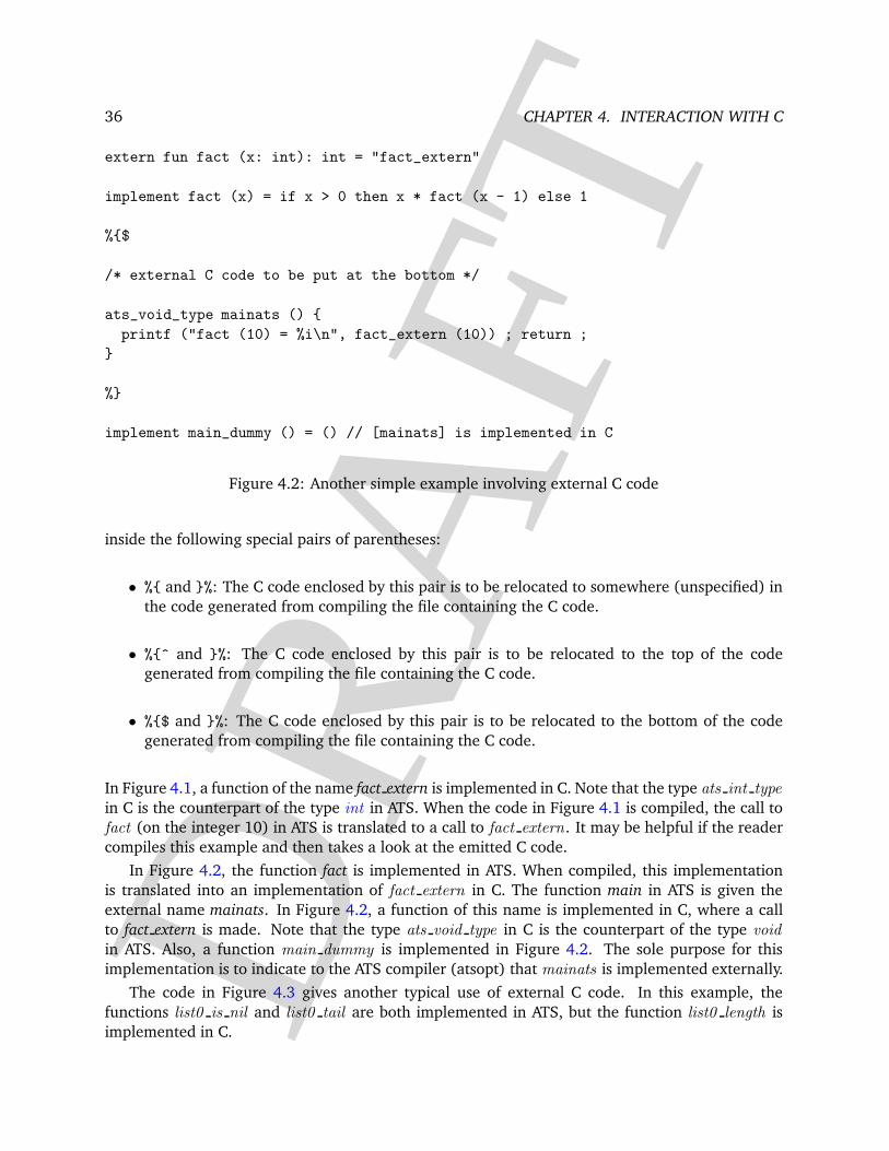
extern fun fact (x: int): int = "fact_extern"

implement fact (x) = if x > 0 then x * fact (x - 1) else 1

%{$

/* external C code to be put at the bottom */

ats_void_type mainats () {

printf ("fact (10) = %i\n", fact_extern (10)) ; return ;

}

%}

implement main_dummy () = () // [mainats] is implemented in C

Figure 4.2: Another simple example involving external C code

inside the following special pairs of parentheses:

• %{ and }%: The C code enclosed by this pair is to be relocated to somewhere (unspecified) in

the code generated from compiling the file containing the C code.

• %{^ and }%: The C code enclosed by this pair is to be relocated to the top of the code

generated from compiling the file containing the C code.

• %{$ and }%: The C code enclosed by this pair is to be relocated to the bottom of the code

generated from compiling the file containing the C code.

In Figure 4.1, a function of the name fact extern is implemented in C. Note that the type ats int type

in C is the counterpart of the type int in ATS. When the code in Figure 4.1 is compiled, the call to

fact (on the integer 10) in ATS is translated to a call to fact extern . It may be helpful if the reader

compiles this example and then takes a look at the emitted C code.

In Figure 4.2, the function fact is implemented in ATS. When compiled, this implementation

is translated into an implementation of fact extern in C. The function main in ATS is given the

external name mainats. In Figure 4.2, a function of this name is implemented in C, where a call

to fact extern is made. Note that the type ats void type in C is the counterpart of the type void

in ATS. Also, a function main dummy is implemented in Figure 4.2. The sole purpose for this

implementation is to indicate to the ATS compiler (atsopt) that mainats is implemented externally.

The code in Figure 4.3 gives another typical use of external C code. In this example, the

functions list0 is nil and list0 tail are both implemented in ATS, but the function list0 length is

implemented in C.

DR

AFT

4.1. EXTERNAL C CODE 37

extern fun list0_is_nil

{a:type} (xs: list0 a): bool = "list0_is_nil"

// end of [extern]

implement list0_is_nil (xs) =

case+ xs of list0_cons _ => true | list0_nil _ => false

exception ListIsEmpty

extern fun list0_tail {a:type} (xs: list0 a): list0 a = "list0_tail"

implement list0_tail (xs) = begin

case+ xs of list0_cons (_, xs) => xs | list0_nil () => $raise ListIsEmpty

end // end of [list0_tail]

extern fun list0_length {a:type} (xs: list0 a): int = "list0_length"

%{

extern ats_ptr_type list0_tail (ats_ptr_type xs) ;

ats_int_type list0_length (ats_ptr_type xs) {

int len = 0 ;

while (1) {

if (list0_is_nil (xs)) break ; xs = list0_tail (xs) ; len += 1 ;

}

return len ;

} /* end of list0_length */

%}

Figure 4.3: An implementation of the list length function in C

DR

AFT


abst@ype T = $extype "T"

extern typedef "list0_cons_pstruct" = list0_cons_pstruct (T, list0 T)

extern fun list0_append (xs: list0 T, ys: list0 T): list0 T = "list0_append"

%{

// how [list0_cons_make] should be implemented is to be

extern list0_cons_pstruct list0_cons_make () ; // discussed later

ats_ptr_type

list0_append (ats_ptr_type xs, ats_ptr_type ys) {

list0_cons_pstruct res0, res, res_nxt ;

if (list0_is_nil (xs)) return ys ;

res0 = res = list0_cons_make () ;

while (1) { /* invariant: [res] is not null */

res->atslab_0 = ((list0_cons_pstruct)xs)->atslab_0 ;

xs = ((list0_cons_pstruct)xs)->atslab_1 ;

if (!xs) break ;

res_nxt = list0_cons_make () ;

res->atslab_1 = res_nxt ; res = res_nxt ;

} /* end of [while] */

res->atslab_1 = ys ; return res0 ;

} /* end of list0_append */

%}

Figure 4.4: An implementation of the list append function in C

4.2 External Types

Suppose that the name someType refers to some type declared in C. Then this type can be referred

to as $extype ”someType” in ATS. On the other hand, one can introduce external names for types in

ATS and then use such names outside ATS. For instance, an external name int int pair is introduced

in the following code to refer to the type @(int, int):

extern typedef "int_int_pair" = @(int, int)

In this case, int int pair is essentially bound to a struct type in C as follows:

typedef struct {

ats_int_type atslab_0 ; ats_int_type atslab_1 ;

} int_int_pair ;

Note that atslab_ is the prefix used by the ATS compiler to form labels for field selection.

Suppose that v is a value of the form C(v1, . . . , vn), where C is a constructor associated with

some datatype and v1, . . . , vn are values of types T1, . . . , Tn, respectively. The value v is represented

DR

AFT

4.3. EXTERNAL VALUES 39

by a pointer to some struct when compiled into C, and the type of this pointer can be referred to

as C pstruct(T1, . . . , Tn) in ATS. As an example, the funtion for appending two lists together is

implemented externally in Figure 4.4. The reader may want to compile this example and then

carefully inspect the emitted C code.

4.3 External Values

Suppose that the name someValue refers to some value in C. Then this value can be referred to as

$extval (T , ”someValue”), where T is the perceived type of this value in ATS. For instance, stdin ref

is defined as a macro in ATS:

macdef stdin_ref = $extval (FILEref, "stdin")

where FILEref is a type in ATS that approximately corresponds to the type FILE∗ in C. Given that

ATS does not support enum types directly, this approach to accessing within ATS values defined in

C also makes it straightforward to define enum types in C and then use them in ATS.

On the other hand, one can introduce external names for values in ATS and then use such

names outside ATS. For instance, an external name one one pair is introduced in the following

code to refer to the value @(1, 1):

extern val "one_one_pair" = @(1, 1)

Note that each external value is registered as a global root for the garbage collector in case garba-

gage collection is performed at run-time.

DR

AFT


DR

AFT

Chapter 5

Programming with Dependent Types

The primary purpose of introducing dependent types into programming is to greatly enhance the

precision in using types to capture program invariants. Generally speaking, dependent types are

types dependent on values of expressions. For instance, bool is a type constructor in ATS that forms

a type bool (b) when applied to a given boolean value b. As this type can only be assigned to the

boolean value b, it is often referred to as a singleton type. Clearly, the meaning of bool (b) depends

on the boolean value b. Similarly, int is a type constructor in ATS that forms a type int(i) when

applied to a given integer i. This type is also a singleton type as it can only be assigned to the

integer value i. Many other examples of dependent types are to be introduced gradually when

this chapter unfolds. In particular, a means for the programmer to declare dependent datatype

constructors is to be presented in Section 5.5.

5.1 Statics

The statics of ATS is a simply typed language. The types and terms in this language are referred to

as sorts and static terms, respectively. Some of the base sorts are given as follows:

• The sort bool is for static terms of boolean values.

• The sort int is for static terms of integer values.

• The sort type is for static terms representing types of size equal to one word.

• The sort t@ype is for static terms representing types of unspecified size.

There are predicative and impredicative sorts: bool and int are predicative while type and t@ype

are impredicative. If a static term is assigned a predicative sort, then then the term is often referred

to as a type index.

There are various constants in the statics. In Figure 5.1, some commonly used static constant

functions are listed together with their sorts. The symbols given inside parentheses are the names

that refer to these constants in the concrete syntax. Many more static constants can be found in

the following file:

$ATSHOME/prelude/basic sta.sats.

41

DR

AFT

42 CHAPTER 5. PROGRAMMING WITH DEPENDENT TYPES

∼ (~) : (int) → int

+ (+) : (int , int) → int

− (-) : (int , int) → int

× (*) : (int , int) → int

÷ (/) : (int , int) → int

> (>) : (int , int) → bool

≥ (>=) : (int , int) → bool

< (<) : (int , int) → bool

≤ (<=) : (int , int) → bool

= (==) : (int , int) → bool

6= (<>) : (int , int) → bool

∨ (||) : (bool , bool ) → bool

∧ (&&) : (bool , bool ) → bool

Figure 5.1: Some commonly used statics constants and their sorts

The names for static constant functions can be overloaded, and an overloaded name is resolved

based on the arity information as well as the information on the sorts of the arguments.

A subset sort is a sort restricted by a predicate. For instance, nat is a subset sort defined as

{a : int | a ≥ 0}. In the concrete syntax, this is done as follows:

sortdef nat = {a: int | a >= 0 }

where sortdef is a keyword in ATS for introducing a sort definition. It is important to not confuse

sorts with subset sorts. The latter can only used to classify quantified static variables. For instance,

the following type (written in the concrete syntax) can be assigned to a function that tests whether

two given natural numbers are equal:

{i,j:nat} (int (i), int (j)) -> bool (i == j)

This type is essentially treated like syntactic sugar for the following one (also written in the concrete

syntax):

{i,j:int | i >= 0; j >= 0} (int (i), int (j)) -> bool (i == j)

5.2 Common Arithmetic and Comparison Functions

Some commonly used arithmetic and comparison functions are listed in Figure 5.2 together with

the dependent types assigned to them. In practice, overloaded names are often used to refer to

these functions. For instance, in the following function definition, > and - are resolved into igt and

isub, respectively:

// [mul_int_int]: the integer mulplication function

fun fact {n:nat} (x: int n): int =

if x > 0 then mul_int_int (x, fact (x - 1)) else 1

DR

AFT

5.3. CONSTRAINT SOLVING 43

ineg : ∀i : int . (int(i)) → int(∼ i)iadd : ∀i1 : int .∀i2 : int . (int(i1), int(i2)) → int(i1 + i2)isub : ∀i1 : int .∀i2 : int . (int(i1), int(i2)) → int(i1 − i2)imul : ∀i1 : int .∀i2 : int . (int(i1), int(i2)) → int(i1 × i2)idiv : ∀i1 : int .∀i2 : int . (int(i1), int(i2)) → int(i1 ÷ i2)igt : ∀i1 : int .∀i2 : int . (int(i1), int(i2)) → bool (i1 > i2)

igte : ∀i1 : int .∀i2 : int . (int(i1), int(i2)) → bool (i1 ≥ i2)ilt : ∀i1 : int .∀i2 : int . (int(i1), int(i2)) → bool (i1 < i2)

ilte : ∀i1 : int .∀i2 : int . (int(i1), int(i2)) → bool (i1 ≤ i2)ieq : ∀i1 : int .∀i2 : int . (int(i1), int(i2)) → bool (i1 = i2)

ineq : ∀i1 : int .∀i2 : int . (int(i1), int(i2)) → bool (i1 6= i2)

Figure 5.2: Some common arithmetic and comparison functions and their dependent types

Note that the symbol int is overloaded: it may represent a dependent type constructor (as in

int(n)) or just a type (for integers). Many more common functions on integers can be found in the

following file:

$ATSHOME/prelude/SATS/integer.sats.

5.3 Constraint Solving

Typechecking in ATS involves generating and solving constraints. As an example, the code below

gives an implementation of the factorial function:

// this definition does not typecheck due to a nonlinear constraint

fun fact {n:nat}

(x: int n): [r:nat] int r = if x > 0 then x * fact (x - 1) else 1

In this implementation, the function fact is assigned the following type:

∀n : nat . int(n) → ∃r : nat. int(r)

which means that fact returns a natural number r when applied to a natural number n. When the

code is typechecked, the following constraints need to be solved:

1. ∀n : nat. n > 0 ⊃ n − 1 ≥ 02. ∀n : nat.∀r1 : nat. n > 0 ⊃ n ∗ r1 ≥ 03. ∀n : nat. n > 0 ⊃ 1 ≥ 0

The first constraint is generated due to the call fact(x − 1), which requires that x − 1 be a natural

number. The second constraint is generated in order to verify that x ∗ fact(x− 1) is a natural num-

ber under the assumption that fact(x − 1) is a natural number. The third constraint is generated

in order to verify that 1 is a natural number. The first and the third constraints can be readily

solved by the constraint solver in ATS, which is based on the Fourier-Motzkin variable elimination

DR

AFT


method (Dantzig and Eaves, 1973). However, the second constraint cannot be handled by the con-

straint solver as it is nonlinear: The constraint cannot be turned into a linear integer programming

problem due to the occurrence of the nonlinear term n ∗ r1. While nonlinear constraints cannot

be handled automatically by the constraint solver in ATS, the programmer is given a means to

verify them by constructing proofs in ATS explicitly. The issue of explicit proof construction is to

be elaborated elsewhere.

Currently, the constraint-solver implemented for ATS/Anairiats makes use of machine-level

arithmetic (in contrast to the standard arithmetic of infinite precision). This is done primarily

for the sake of efficiency. In the presence of machine-level arithmetic overflow, results returned by

the constraint-solver are likely to be incorrect. While such cases can be readily constructed, their

appearances in practice seem exceedingly rare (and the author has not yet encountered one to this

date).

5.4 A Simple Example: Dependent Types for Debugging

Given a non-negative integer x, the integer square root of x is the greatest integer i satisfying

i ∗ i ≤ x. In Figure 5.3, an implementation of the integer square root function is given based on

the method of binary search. This implementation passes typechecking, but it seems to be looping

forever when tested. Instead of going into the standard routine of debugging (e.g., by inserting

calls to some printing functions), we now attempt to identify the cause for non-termination by

trying to prove the termination of the function search through the use of dependent types.

fn isqrt (x: int): int = let

fun search (x: int, l: int, r: int): int = let

val diff = r - l

in

case+ 0 of

| _ when diff > 0 => let

val m = l + (diff / 2)

in

// [div_int_int] is the integer division function

if div_int_int (x, m) < m then search (x, l, m) else search (x, m, r)

end // end of [if]

| _ => l

end // end of [search]

in

search (x, 0, x)

end // end of [isqrt]

Figure 5.3: A buggy implementation of the integer square root function

The function search in Figure 5.3 is assigned the type (int , int , int) → int , meaning that search

takes three integers as its arguments and returns an integer as its result. On the other hand, the

programmer may have thought that the function search should possess the following invariants (if

DR

AFT

5.4. A SIMPLE EXAMPLE: DEPENDENT TYPES FOR DEBUGGING 45

fn isqrt {x:nat} (x: int x): int = let

fun search {x,l,r:nat | l < r} .<r-l>.

(x: int x, l: int l, r: int r): int = let

val diff = r - l

in

case+ 0 of

| _ when diff > 1 => let

val m = l + (diff / 2)

in

// [div_int_int] is the integer division function

if div_int_int (x, m) < m then search (x, l, m) else search (x, m, r)

end // end of [if]

| _ => l

end // end of [search]

in

if x > 0 then search (x, 0, x) else 0

end // end of [isqrt]

Figure 5.4: A fixed dependently typed implementation corresponding to the one in Figure 5.3

implemented correctly):

1. l ∗ l ≤ x < r ∗ r must hold when search(x, l, r) is called.

2. Assume l ∗ l ≤ x < r ∗ r for some integers x, l, r. If a recursive call search(x, l′, r′) for some

integers l′ and r′ is encountered in the body of search(x, l, r), then r′ − l′ < r − l must hold.

This invariant implies that search is terminating.

Though the first invariant can be captured in the type system of ATS, it is somewhat involved to do

so due to the need for handling nonlinear constraints. Instead, the following dependent function

type is assigned to search in Figure 5.4, which captures a weaker invariant stating that l < r must

hold when search(x, l, r) is called:

search : ∀x : nat .∀l : nat .∀r : nat .(l < r) ⊃ 〈r − l〉 ⇒ ((int(x), int(l), int(r)) → int)

It should not be difficult to relate this type to the concrete syntax representing it in the code. Note

that the term 〈r − l〉, which corresponds to the concrete syntax .<r-l>., represents a termination

metric needed for verifying the second invariant. More details on termination metrics are to be

given later.

With search being assigned the above dependent function type, the implementation in Fig-

ure 5.3 needs to be modified in order to pass typechecking. The modifications can be readily

identified by comparing the code in Figure 5.3 to the the code in Figure 5.4, and the reader is

strongly encouraged to do so and then figure out the reason for these modifications.

DR

AFT


5.5 Dependent Datatypes

The feature of datatypes in ATS is directly adopted from ML. In ATS, there is even a means for the

programmer to introduce dependent datatypes (or more precisely, dependent datatype construc-

tors). For instance, the datatype constructor list in ATS is declared as follows:

datatype list (t@ype+, int) =

| {a:t@ype} list_nil (a, 0)

| {a:t@ype} {n:nat} list_cons (a, n+1) of (a, list (a, n))

The syntax indicates that list is a type constructor that forms a type list(T, I) when applied to a

type T (of sort t@ype) and an integer I. The sort t@ype means that the size of T is unspecified.

The plus sign following t@ype states that list is covariant in its first argument, that is, list(T1, n) is a

subtype of list(T2, n) if T1 is a subtype of T2. There are two data constructors list nil and list cons

associated with list , which are assigned the following types:

list nil : ∀a : t@ype. () → list(a, 0)list cons : ∀a : t@ype∀n : int . (a, list(a, n)) → list(a, n + 1)

Given a type T and an integer I, it is clear that the type list(T, I) is for lists of length I in which

each element is of type T . The above declaration for list can also be given as follows in a more

succint manner:

datatype list (a:t@ype+, int) =

| list_nil (a, 0) | {n:nat} list_cons (a, n+1) of (a, list (a, n))

// list_length<a>: {n:nat} list (a, n) -> int (n)

fn{a:t@ype} list_length {n:nat} (xs: list (a, n)): int (n) = let

// loop: {i,j:nat} (list (a, i), int (j)) -> int (i+j)

fun loop {i,j:nat} .. // .. is a termination metric

(xs: list (a, i), j: int j): list (i+j) = begin

case+ xs of list_cons (_, xs) => loop (xs, j+1) | list_nil () => j

end // end of [loop]

in

loop (xs, 0)

end // end of [list_length]

Figure 5.5: A tail-recursive implementation of the list length function

In Figure 5.5, an implementation of the list length function is given. The function template

list length can be instantiated with a type T (of unspecified size) to yield a function list length〈T 〉of the following function type:

∀n : nat . list(T, n) → int(n)

which clearly indicates that the value returned by the function list length〈T 〉 is the length of its

argument.

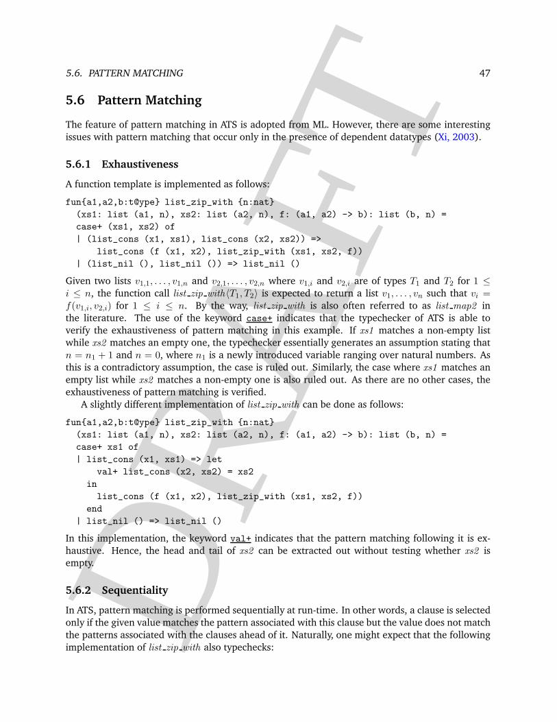
DR

AFT

5.6. PATTERN MATCHING 47

5.6 Pattern Matching

The feature of pattern matching in ATS is adopted from ML. However, there are some interesting

issues with pattern matching that occur only in the presence of dependent datatypes (Xi, 2003).

5.6.1 Exhaustiveness

A function template is implemented as follows:

fun{a1,a2,b:t@ype} list_zip_with {n:nat}

(xs1: list (a1, n), xs2: list (a2, n), f: (a1, a2) -> b): list (b, n) =

case+ (xs1, xs2) of

| (list_cons (x1, xs1), list_cons (x2, xs2)) =>

list_cons (f (x1, x2), list_zip_with (xs1, xs2, f))

| (list_nil (), list_nil ()) => list_nil ()

Given two lists v1,1, . . . , v1,n and v2,1, . . . , v2,n where v1,i and v2,i are of types T1 and T2 for 1 ≤i ≤ n, the function call list zip with〈T1, T2〉 is expected to return a list v1, . . . , vn such that vi =f(v1,i, v2,i) for 1 ≤ i ≤ n. By the way, list zip with is also often referred to as list map2 in

the literature. The use of the keyword case+ indicates that the typechecker of ATS is able to

verify the exhaustiveness of pattern matching in this example. If xs1 matches a non-empty list

while xs2 matches an empty one, the typechecker essentially generates an assumption stating that

n = n1 + 1 and n = 0, where n1 is a newly introduced variable ranging over natural numbers. As

this is a contradictory assumption, the case is ruled out. Similarly, the case where xs1 matches an

empty list while xs2 matches a non-empty one is also ruled out. As there are no other cases, the

exhaustiveness of pattern matching is verified.

A slightly different implementation of list zip with can be done as follows:



case+ xs1 of

| list_cons (x1, xs1) => let

val+ list_cons (x2, xs2) = xs2

in


end

| list_nil () => list_nil ()

In this implementation, the keyword val+ indicates that the pattern matching following it is ex-

haustive. Hence, the head and tail of xs2 can be extracted out without testing whether xs2 is

empty.

5.6.2 Sequentiality

In ATS, pattern matching is performed sequentially at run-time. In other words, a clause is selected

only if the given value matches the pattern associated with this clause but the value does not match

the patterns associated with the clauses ahead of it. Naturally, one might expect that the following

implementation of list zip with also typechecks:

DR

AFT




case+ (xs1, xs2) of

| (list_cons (x1, xs1), list_cons (x2, xs2)) =>


| (_, _) => list_nil ()

This, however, is not the case. In ATS, typechecking clauses is done nondeterministically (rather

than sequentially). In this example, the second clause fails to typecheck as it is done without

assuming that the given value does not match the pattern associated with the first clause. The

second clause can be modified as follows:

| (_, _) =>> list_nil ()

The use of =>> (in place of =>) indicates to the typechecker that this clause needs to be typechecked

under the assumption that the given value does not match the pattern associated with each pre-

vious clause. Hence, when the modified second clause is typechecked, it can be assumed that the

value that matches the pattern ( , ) must match one of the following:

(list cons( , ), list nil()) (list nil(), list cons( , )) (list cons( , ), list cons( , ))

This assumption allows typechecking to succeed.

5.7 Program Termination Verification

A termination metric is a tuple of natural numbers 〈m1, . . . ,mn〉, and the standard lexicographic

ordering on natural numbers is used to order such tuples. In ATS, termination metrics can be

supplied (by the programmer) for verifying whether recursively defined functions are terminating,

and this feature plays a crucial role in supporting the paradigm of programming with theorem

proving.

In the following example, a singleton metric 〈n〉 is supplied to verify that the recursive function

fact is terminating, when n is the value of the argument of fact :

fun fact {n:nat} .<n>. (x: int n): int = if x > 0 then x * fact (x-1) else 1

The metric attached to the call fact(x − 1) is 〈n − 1〉, which is obviously less than 〈n〉.A more difficult and also more interesting example is given as follows, where the MacCarthy’s

91-function is implemented:

fun f91 {i:int} .<max(101-i,0)>. (x: int i)

: [j:int | (i <= 100 && j == 91) || (i > 100 && j == i-10)] int j =

if x > 100 then x-10 else f91 (f91 (x+11))

It is clear from the dependent type assigned to f91 that the function always returns 91 when

applied to an integer less than or equal 100. The metric supplied to verify the termination of f91

is 〈max(101 − i, 0)〉, where i is the value of the argument of f91 .

The following code implements the Ackermann function, which is well-known for being recur-

sive but not primitive recursive:

DR

AFT

5.7. PROGRAM TERMINATION VERIFICATION 49

fun ack {m,n:nat} .<m,n>. (x: int m, y: int n): [r:nat] int r =

if x > 0 then

if y > 0 then ack (x - 1, ack (x, y - 1)) else ack (x - 1, 1)

else y + 1

The metric supplied for verifying the termination of ack is a pair 〈m,n〉, where m and n are the

values of the arguments of ack .

In the following example, isEven and isOdd are defined mutually recursively:

fun isEven {n:nat} .<2*n>. (x: int n): bool =

if x > 0 then isOdd (x - 1) else true

and isOdd {n:nat} .<2*n+1>. (x: int n): bool =

not (isEven x)

The metrics supplied for verifying the termination of isEven and isOdd are 〈2 ∗ n〉 and 〈2 ∗ n + 1〉,respectively, when n is the value of the argument of isEven and also the value of the argument of

isOdd . Clearly, if the metrics 〈n, 0〉 and 〈n, 1〉 are supplied for isEven and isOdd , respectively, the

termination of these two functions can also be verified. Note that it is required that the metrics for

mutually recursively defined functions be of the same length.

DR

AFT


DR

AFT

Chapter 6

Programming with Theorem Proving

The paradigm of programming with theorem proving is rich and broad, and it is probably the most

innovative feature in ATS. It will become clear later that this feature plays an indispensable role in

ATS to support safe manipulation of resources. In this chapter, we mainly give an introduction to

programming with theorem proving by presenting a few examples, explaining some motivations

behind this programming paradigm as well as demonstrating a means to achieve it in ATS.

extern fun{a:t@ype} list_append {n1,n2:nat}

(xs: list (a, n1), ys: list (a, n2)): list (a, n1+n2)

// [concat] does not typecheck due to nonlinear constraints

fun{a:t@ype} concat {m,n:nat}

(xss: list (list (a, n), m)): list (a, m * n) =

case+ xss of

| list_cons (xs, xss) => list_append<a> (xs, concat xss)

| list_nil () => list_nil ()

Figure 6.1: An implementation of list concatenation that does not typecheck

6.1 Nonlinear Constraint Avoidance

A function template concat is implemented in Figure 6.1. Given a list xss of length m in which

each element is of type list(T, n), concat〈T 〉(xss) constructs a list of type list(T,m ∗ n). When the

first pattern matching clause in the code for concat is typechecked, a constraint is generated that

is essentially like the following one:

∀m : nat .∀m1 : nat .∀n : nat .m = m1 + 1 ⊃ n + (m1 ∗ n) = m ∗ n

This contraint may look simple, but it is rejected by the ATS constraint solver as it contains nonlin-

ear terms (e.g., m1 ∗ n and m ∗ n). In order to overcome the limitation, theorem-proving can be

employed.

51

DR

AFT

52 CHAPTER 6. PROGRAMMING WITH THEOREM PROVING

dataprop MUL (int, int, int) =

| {n:int} MULbas (0, n, 0)

| {m,n,p:int | m >= 0} MULind (m+1, n, p+n) of MUL (m, n, p)

| {m,n,p:int | m > 0} MULneg (~m, n, ~p) of MUL (m, n, p)

Figure 6.2: A dataprop for encoding integer multiplication

A dataprop declaration is given in 6.2. A dataprop is like a datatype, but it can only be assigned

to proof values (or proofs for short). In ATS, after a program passes typechecking, a procedure

called proof erasure can be performed to erase all the parts in the program that are related to proofs.

In particular, there is no proof construction at run-time. The constructors MULbas, MULind and

MULneg associated with MUL essentially correspond to the following equations in a definition of

integer multiplication (based on integer addition):

0 ∗ n = 0 (m + 1) ∗ n = m ∗ n + n for m >= 0 (−m) ∗ n = −(m ∗ n) for m > 0

Given integers m,n, p, if MUL(m,n, p) is inhabited, that is, if it can be assigned to some proof

value, then m ∗ n equals p.

fun{a:t@ype} concat {m,n:nat}

(xss: list (list (a, n), m)): [p:nat] (MUL (m, n, p) | list (a, p)) =

case+ xss of

| list_cons (xs, xss) => let

val (pf | res) = concat xss

in

(MULind pf | list_append<a> (xs, res))

end

| list_nil () => (MULbas () | list_nil ())

Figure 6.3: An implementation of list concatenation that does typecheck

In Figure 6.3, another implementation of the function template concat is given that avoids the

generation of nonlinear constraints. Given a type T , concat〈T 〉 is assigned the following type in

this implementation:

∀m : nat .∀n : nat . list(list(T, n),m) → ∃p : nat . (MUL(m,n, p) | list(T, p))

Given a list xss of type list(list(T, n),m), concat (v) returns a pair (pf | res) such that pf is a proof

of type MUL(m,n, p) for some p and res is a list of type list(T, p). In other words, pf acts a witness

to p = m ∗ n. After proof erasure is performed, the implementation in Figure 6.3 is essentially

translated into the one in Figure 6.1.

In Figure 6.4, a dataprop FACT is declared to encode the following definition of the factorial

function:

fact(0) = 1 fact(n + 1) = fact(n) ∗ (n + 1) for n > 0

Given integers n and r, if FACT (n, r) is inhabited, then fact(n) equals r.

DR

AFT

6.1. NONLINEAR CONSTRAINT AVOIDANCE 53

dataprop FACT (int, int) =

| FACTbas (0, 1)

| {n:nat;r,r1:int} FACTind (n+1, r1) of (FACT (n, r), MUL (r, n+1, r1))

infixl imul2 // left-associative infix operator

extern fun imul2 {m,n:int}

(m: int m, n: int n): [p:int] (MUL (m, n, p) | int p)

extern fun fact {n:nat} (n: int n): [r:int] (FACT (n, r) | int r)

implement fact (n) = // a non-tail-recursive implementation

if n > 0 then let

val (pf | r) = fact (n-1); val (pf_mul | r1) = r imul2 n

in

(FACTind (pf, pf_mul) | r1)

end else begin

(FACTbas () | 1)

end // end of [if]

implement fact (n) = let // a tail-recursive implementation

fun loop {n,i,r:int | 0 < i; i <= n+1} .<n+1-i>.

(pf: FACT (i-1, r) | n: int n, i: int i, r: int r)

: [r:int] (FACT (n, r) | int r) =

if i > n then (pf | r) else let

val (pf_mul | r1) = r imul2 i; prval pf1 = FACTind (pf, pf_mul)

in

loop (pf1 | n, i + 1, r1)

end // end of [if]

in

loop (FACTbas () | n, 1, 1)


Figure 6.4: A fully verified implemenation of the factorial function

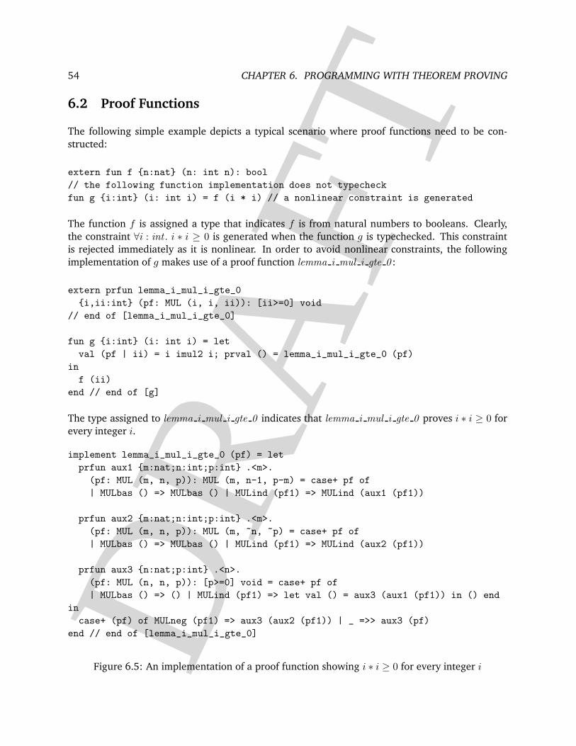
DR

AFT


6.2 Proof Functions

The following simple example depicts a typical scenario where proof functions need to be con-

structed:

extern fun f {n:nat} (n: int n): bool

// the following function implementation does not typecheck

fun g {i:int} (i: int i) = f (i * i) // a nonlinear constraint is generated

The function f is assigned a type that indicates f is from natural numbers to booleans. Clearly,

the constraint ∀i : int . i ∗ i ≥ 0 is generated when the function g is typechecked. This constraint

is rejected immediately as it is nonlinear. In order to avoid nonlinear constraints, the following

implementation of g makes use of a proof function lemma i mul i gte 0 :

extern prfun lemma_i_mul_i_gte_0

{i,ii:int} (pf: MUL (i, i, ii)): [ii>=0] void

// end of [lemma_i_mul_i_gte_0]

fun g {i:int} (i: int i) = let

val (pf | ii) = i imul2 i; prval () = lemma_i_mul_i_gte_0 (pf)

in

f (ii)

end // end of [g]

The type assigned to lemma i mul i gte 0 indicates that lemma i mul i gte 0 proves i ∗ i ≥ 0 for

every integer i.

implement lemma_i_mul_i_gte_0 (pf) = let

prfun aux1 {m:nat;n:int;p:int} .<m>.

(pf: MUL (m, n, p)): MUL (m, n-1, p-m) = case+ pf of

| MULbas () => MULbas () | MULind (pf1) => MULind (aux1 (pf1))

prfun aux2 {m:nat;n:int;p:int} .<m>.

(pf: MUL (m, n, p)): MUL (m, ~n, ~p) = case+ pf of

| MULbas () => MULbas () | MULind (pf1) => MULind (aux2 (pf1))

prfun aux3 {n:nat;p:int} .<n>.

(pf: MUL (n, n, p)): [p>=0] void = case+ pf of

| MULbas () => () | MULind (pf1) => let val () = aux3 (aux1 (pf1)) in () end

in

case+ (pf) of MULneg (pf1) => aux3 (aux2 (pf1)) | _ =>> aux3 (pf)

end // end of [lemma_i_mul_i_gte_0]

Figure 6.5: An implementation of a proof function showing i ∗ i ≥ 0 for every integer i

DR

AFT

6.2. PROOF FUNCTIONS 55

prfun lemma_for_matrix_subscripting

{m,n:nat} {i:nat | i < m} {mn,p:int} .<m>.

(pf1: MUL (m, n, mn), pf2: MUL (i, n, p)): [p+n <= mn] void = let

prval MULind (pf11) = pf1

in

sif i < m-1 then begin

lemma_for_matrix_subscripting {m-1,n} {i} (pf11, pf2)

end else let // i = m-1

prval () = mul_isfun (pf11, pf2)

in

// empty

end // end of [sif]

end // end of [lemma_for_matrix_subscripting]

Figure 6.6: A proof function needed in the implementation of matrix subscripting

An implementation of lemma i mul i gte 0 is given in Figure 6.5, where the auxiliary proof

functions aux1 , aux2 and aux3 are given the following types:

aux1 : ∀m : nat .∀n : int .∀p : int . MUL(m,n, p) → MUL(m,n − 1 , p − m)aux2 : ∀m : nat .∀n : int .∀p : int . MUL(m,n, p) → MUL(m,−n,−p)aux3 : ∀n : nat .∀p : int . MUL(n, n, p) → (p ≥ 0) ∧ void

In other words, the following is established by these proof functions:

aux1 proves ∀m : nat .∀n : int . m ∗ (n − 1) = m ∗ n − maux2 proves ∀m : nat .∀n : int . m ∗ (−n) = −(m ∗ n)aux3 proves ∀n : nat .n ∗ n ≥ 0

Matrix Implementation A realistic example involving proof construction can be found in the

following file:

$ATSHOME/prelude/DATS/matrix.dats

where matrices are implemented in ATS. A 2-dimension matrix of dimension m × n in ATS is

represented a 1-dimension array of size m · n in the row-major format. Given natural numbers iand j satisfying i < m and j < n, the element in the matrix indexed by (i, j) is the element in the

array indexed by i · n + j. This means that the following theorem is needed in order to implement

matrix subscripting (without resorting to run-time array bounds checking):

∀m : nat .∀n : nat .∀i : nat .∀j : nat . (i < m ∧ j < n) ⊃ (i · n + j < m · n)

As linear constraints are handled automatically in ATS, this theorem is equivalent to the following

one,

∀m : nat .∀n : nat .∀i : nat . (i < m) ⊃ (i · n + n ≤ m · n)

which is encoded and proven in Figure 6.6.

DR

AFT


datasort intlst = intlst_nil of () | intlst_cons of (int, intlst)

dataprop int_intlst_lte (int, intlst) =

| {i:int} {x:int | i <= x} {xs:intlst}

int_intlst_lte_cons (i, intlst_cons (x, xs)) of int_intlst_lte (i, xs)

| {i:int} int_intlst_lte_nil (i, intlst_nil ())

// if i <= j and j <= x for each x in xs, then i <= x for each x in xs

prfun int_intlst_lte_lemma

{i,j:int | i <= j} {xs: intlst} .<xs>.

(pf: int_intlst_lte (j, xs)): int_intlst_lte (i, xs) = case+ pf of

| int_intlst_lte_cons (pf) => int_intlst_lte_cons (int_intlst_lte_lemma pf)

| int_intlst_lte_nil () => int_intlst_lte_nil ()

// end of [int_intlst_lte_lemma]

prfun intlst_lower_bound_lemma

{xs:intlst} .<xs>. (): [x_lb:int] int_intlst_lte (x_lb, xs) =

scase xs of

| intlst_cons (x1, xs1) => let

prval [x1_lb:int] pf1 = intlst_lower_bound_lemma {xs1} ()

in

sif x1 <= x1_lb then begin // static conditional

int_intlst_lte_cons (int_intlst_lte_lemma {x1, x1_lb} (pf1))

end else begin

int_intlst_lte_cons (pf1)

end // end of [sif]

end // end of [intlst_cons]

| intlst_nil () => int_intlst_lte_nil {0} ()

// end of [intlst_lower_bound_lemma]

Figure 6.7: A simple example involving datasort declaration

DR

AFT

6.3. DATASORTS 57

6.3 Datasorts

So far, the type indexes appearing in the presented examples are all of some built-in sorts (e.g., bool ,

int). In ATS, it is also possible for the programmer to introduce sorts by datasort declaration. As

an example, a datasort intlst is first declared in Figure 6.7, and each index of this sort represents a

sequence of integers. Subsequently, a dataprop int intlst lte is declared, which captures the relation

stating that a given integer is less than or equal to each integer in a given integer sequence.

The first proof function int intlst lte lemma in Figure 6.7 proves that an integer i is less than or

equal to x for each integer x in a given integer sequence if i ≤ j and j ≤ x for each integer x in the

sequence. Note that the termination metric for this proof function is 〈xs〉, where xs ranges over

static terms of the sort intlst that are compared according to the substructural ordering: A term is

strictly less than another term if the former is a proper subterm of the latter.

The next proof function intlst lower bound lemma in Figure 6.7 proves that for each integer

sequence, there is a lower bound xlb for the sequence, that is, x ≤ xlb holds for each x in the

sequence. Please notice the use of sif and scase in this example. In constrast to if, sif is used to

construct a static conditional expression where the condition is a static expression of the sort bool .

In an analogous manner, scase is used to construct a static case-expression where the expression

being matched against is static. Each pattern used for matching in a static case-expression must be

simple, that is, it must be of the form of a constructor being applied to variables.

DR

AFT


DR

AFT

Chapter 7

Programming with Linear Types

The paradigm of programming with theorem proving plays an indispensable role in making linear

types available for practical use in ATS. In this chapter, we present some examples of resource

manipulation involving linear types. In particular, we demonstrate that ATS not only supports

flexible uses of pointers but can also guarantee based on its type system that such uses are safe.

7.1 Safe Memory Access through Pointers

In ATS, a linear prop is referred to as a view and a linear type, which is often a type combined

with a view, is referred to as a viewtype. A commonly used view constructor is @ (infix), which

forms a view T@L when applied to a type T and a memory location L. If a proof of the view T@Lis available, then it is guaranteed that a value of the type T is stored at the location L. In the

following presentation, views of the form T@L is often referred to as @-views. As an example, the

following function templates ptr get0 and ptr set0, which reads and writes through a given pointer,

are assigned types containing @-views:

fun{a:t@ype} ptr_get0 {l:addr} (pf: a @ l | p: ptr l): @(a @ l | a)

fun{a:t@ype} ptr_set0 {l:addr} (pf: a? @ l | p: ptr l, x: a): @(a @ l | void)

Note that ptr is a type constructor that forms a type ptr (L) when applied to a static term L of the

sort addr, and the only value of the type ptr (L) is the pointer that points to the location represented

by L.

Given a type T , the function ptr get0 〈T 〉 is assigned the following type:

∀l : addr . (T@l | ptr (l)) → (T@l | T )

This type indicates that the function ptr get0 〈T 〉 returns a proof of the view T@L and a value of

the type T when applied to a proof of the view T@L and a pointer of the type ptr (L) for some

L. Intuitively speaking, a proof of the view T@L, which is a form of resource as T@L is linear,

is consumed when it is passed to ptr get0 〈T 〉, and another proof of the view T@L is generated

when ptr get0 〈T 〉 returns. Notice that a proof of the view T@L must be returned for otherwise

subsequent accesses to the memory location L become impossible.

Similarly, the function ptr set0 〈T 〉 is assigned the following type:

∀l : addr . (T ?@l | ptr(l)) → (T@l | void)

59

DR

AFT

60 CHAPTER 7. PROGRAMMING WITH LINEAR TYPES

fn{a:t@ype} swap0 {l1,l2:addr}

(pf1: a @ l1, pf2: a @ l2 | p1: ptr l1, p2: ptr l2)

: (a @ l1, a @ l2 | void) = let

val (pf1 | tmp1) = ptr_get0<a> (pf1 | p1)

val (pf2 | tmp2) = ptr_get0<a> (pf2 | p2)

val (pf1 | ()) = ptr_set0<a> (pf1 | p1, tmp2)

val (pf2 | ()) = ptr_set0<a> (pf2 | p2, tmp1)

in

(pf1, pf2 | ())

end // end of [swap0]

Figure 7.1: A function for swapping memory contents (I)

Note that T ? is a type for values of size sizeof (T ) (that are assumed to be uninitialized). The

function ptr set0 〈T 〉 returns a proof of the view T@L when applied to a proof of the view T ?@L,

a pointer of the type ptr (L) and a value of the type T . The use of the view T ?@L indicates that the

memory location at L is assumed to be uninitialized when ptr set0 〈T 〉 is called.

In Figure 7.1, a function template swap0 is implemented for swapping memory contents at two

given locations. Compared to a corresponding implementation in C, the verbosity of this one in

ATS is evident. In particular, the need for threading linear proofs through calls to functions that

make use of resources often results in a significant amount of code to be written. We now introduce

some special syntax to significantly alleviate the need for such code.

The function templates ptr get1 and ptr set1 are given the following types:

fun{a:t@ype} ptr_get1 {l:addr} (pf: !a @ l >> a @ l | p: ptr l): a

fun{a:t@ype} ptr_set1 {l:addr} (pf: !a? @ l >> a @ l | p: ptr l, x: a): void

Clearly, for each type T , the function ptr get1 〈T 〉 is assigned the following type:

∀l : addr . (!T@l ≫ T@l | ptr (l)) → T

Given a linear proof pf of the view T@L for some L and a pointer p of the type ptr (L), the function

call ptr get1 〈T 〉(pf , p) is expected to return a value of the type T . However, the proof pf is not

consumed. Instead, it is still a proof of the view T@L after the function call. Similarly, the function

ptr set1 〈T 〉 is assigned the following type:

∀l : addr . (!T ?@l ≫ T@l | ptr (l), T ) → void

Given a linear proof pf of the view T ?@L for some L, a pointer p of the type ptr (L) and a value

x of the type T , the function call ptr set1 〈T 〉(pf , p, x) is expected to return the void value while

changing the view of pf from T ?@L to T@L. In general, if f is given a type of the following form

for some views V1 and V2:

(. . . , !V1 ≫ V2, . . .) → . . .

then a function call f(. . . , pf , . . .) on some proof variable pf of the view V1 is to change the view of

pf into V2 upon its return. In the case where V1 and V2 are the same, !V1 ≫ V2 can simply be written

DR

AFT

7.2. LOCAL VARIABLES 61


(pf1: !a @ l1, pf2: !a @ l2 | p1: ptr l1, p2: ptr l2): void = let

val tmp = ptr_get1<a> (pf1 | p1)

in

ptr_set1<a> (pf1 | p1, ptr_get1<a> (pf2 | p2)); ptr_set1<a> (pf2 | p2, tmp)


Figure 7.2: A function for swapping memory contents (II)


(pf1: !a @ l1, pf2: !a @ l2 | p1: ptr l1, p2: ptr l2): void = let

val tmp = !p1

in

!p1 := !p2; !p2 := tmp


Figure 7.3: A function for swapping memory contents (III)

as !V1. As an example, a function swap1 for swapping the contents at two given memory locations

is implemented in Figure 7.2, where the function templates ptr get1 and ptr set1 are employed.

Clearly, this implementation is considerably cleaner when compared to the one in Figure 7.1.

A further simplied implementation of swap1 is given in Figure 7.3. Given a pointer p of the

type ptr (L) for some L, !p yields the value stored at the memory location L. The typechecker first

searches for a proof of the view T@L for some T among all available proofs when typechecking

!p; if such a proof pf is found, then !p is essentially elaborated into ptr get1 (pf | p) and then

typechecked. As !p is a left-value, it can also be used to form an assignment like !p := v. The

typechecker elaborates !p := v into ptr set1 (pf | p, v) for the sake of typechecking if a proof of the

view T@L can be found among all available proofs.

7.2 Local Variables

Local variables within a function are stored in the frame allocated for the function when it is called.

In ATS, it is guaranteed by the type system that no local variables stored in the frame of a function

can be accessed once the call to the function returns. In other words, the issue of a local variable

escaping its legal scope is completely prevented by the type system of ATS.

In Figure 7.4, a local variable is used in an implementation of the factorial function. Given an

address L, the function loop in the implementation takes a proof of int@L, an integer and a pointer

to L, and it keeps updating the integer value stored at L until it exits. When the local variable res

is introduced, a static address of the same name is introduced implicitly. In addition, a proof of the

view int?@res is introduced implicitly, and this proof is often referred to as the proof associated

with the dynamic variable res . In order to guarantee that res can never be accessed outside its

legal scope, the type system requires that at the end of the legal scope of res , the view of the proof

associated with res must be the same as the view originally assigned to the proof.

DR

AFT



fun loop {l:addr} (pf: !int @ l | x: int, p_res: ptr l): void =

if x > 0 then (!p_res := !p_res * x; loop (pf | x-1, p_res)) else ()

var res: int = 1

in

loop (view@ (res) | x, &res); res


Figure 7.4: An implementation of the factorial function that makes use of a local variable

The expression &res , which is assigned the type ptr(res), represents the pointer to res , and the

expression view@(res) refers to the implicitly introduced proof that is associated with res . Note

that the view of this proof changes from int?@res into int@res once res is initialized with the

integer 1.

If the following line is used to introduce res instead:

var res: int // uninitialized

then the proof associated with res is assigned the view int?@res when it is passed as a proof

argument to the function loop, resulting in a type error.

It is also possible to employ the following syntax to introduce the local variable res in Figure 7.4:

var res: int with pf_res = 1

In addition to introducing res , the form of syntax also introduces pf res as an alias of view@(res),thus allowing the former to be used in place of the latter.

The implementation of the factorial function in Figure 7.4 should be compared with the one in

Figure 1.3, where a reference (instead of a local variable) is created to hold intermediate results

during computation. As references are allocated on heap and the memory for storing each refer-

ence can only be safely reclaimed through GC, using local variables, if possible, is often preferred

to using references.

7.3 Memory Allocation on Stack

ATS supports memory being allocated in the stack frame of a function at run-time. Like in the case

of local variables, the type system of ATS guarantees that no memory allocated in the stack frame

of a function can be accessed after the call to the function returns.

As an example, the code in Figure 7.5 prints out the current time in certain string format.

First, a call to the function time get is issued to obtain the number of seconds since the Epoch (the

starting moment of the first of January, 1970 measured in UTC time). Then a buffer of N bytes

is allocated in the stack frame of the current function call, where N equals some integer constant

CTIME BUFLEN defined to be greater than or equal to 26. The following line in Figure 7.5

indicates a buffer of N bytes is allocated in the current stack frame at run-time:

var !p_buf with pf_buf = @[byte][CTIME_BUFLEN]()

DR

AFT

7.4. CALL-BY-REFERENCE 63

implement main () = let

// obtain the number of seconds since the Epoch

var ntick: time_t = time_get ()

// allocate memory in the stack frame

var !p_buf with pf_buf = @[byte][CTIME_BUFLEN]()

// turn the number into a string representation

val _(*p_buf*) = ctime_r (pf_buf | ntick, p_buf)

val () = print (!p_buf) // print out the string representation

in

pf_buf := bytes_v_of_strbuf_v (pf_buf) // change the view of pf_buf

// to @[byte][CTIME_BUFEN] @ p_buf as is expected by the typechecker


Figure 7.5: An example involving memory allocation in stack frame at run-time

The dynamic variable p buf is assigned the type ptr(p buf ), where p buf is overloaded to refer

to the starting address of the allocated buffer, and the proof variable pf buf is given the view

@[byte?][N ]@p buf , which states that the allocated buffer is uninitialized. In general, given a type

T , an integer I and an address L, the type @[T ][I] is for an array of I values of type T and the view

@[T ][I]@L indicates that such an array is stored at L. If the allocated buffer needs to be initialized

with some byte value b, the following line can be used:

var !p_buf with pf_buf = @[byte][CTIME_BUFLEN](b)

In this case, the view assigned to pf buf is @[byte][N ]@p buf , meaning that the buffer is initialized.

The function ctime r , which is a reentrant version of the function ctime, turns a time represented

as the number of seconds since the Epoch into some string representation and then stores the string

inside the buffer to which its last argumnent points. After the call to ctime r returns, the view of

pf buf changes into strbuf (N, I)@p buf for some natural number I, meaning that a string (i.e., a

sequence of bytes ending with the null byte) of length I is stored in the buffer. After this string is

printed out, the view of pf buf needs to be changed into @[byte?][N ]@p buf , and this is done by

calling the proof function bytes v of strbuf v .

7.4 Call-By-Reference

The feature of call-by-reference in ATS is similar to the corresponding one in C++. What is special

in ATS is the way in which this feature is handled by the type system. In general, if f is given a

type of the following form for some viewtypes VT 1 and VT 2:

(. . . ,&VT 1 ≫ VT 2, . . .) → . . .

then a function call f(. . . , x , . . .) on some variable x of the viewtype VT 1 is to change the viewtype

of x into VT 2 upon its return. In the case where VT 1 and VT 2 are the same, &VT 1 ≫ VT 2 can

simply be written as &VT 1. The variable x may be replaced with other forms of left-values.

DR

AFT



fun loop {l:addr} (x: int, res: &int): void =

if x > 0 then (res := res * x; loop (x-1, res)) else ()

var res: int = 1

in

loop (x, res); res


Figure 7.6: An implementation of the factorial function that makes use of call-by-reference

As an example, an implementation of the factorial function is given in Figure 7.6 that makes

use of call-by-reference. Note that if the line for introducing the variable res in the implementation

is replaced with the following one:

val res: int = 1 // [res] is now a value, not a variable!

then a type error should occurs as res is no longer a left-value when it is passed as an argument to

loop. For instance, the reason for introducing ntick as a variable in Figure 7.5 is precisely due to

ctime r requiring that its first non-proof argument be passed as a reference.

The implementation in Figure 7.6 should be compared with the one in Figure 7.4. These two

are really the same implementation, but the latter is clearly cleaner than the former in terms of the

syntax being used.

7.5 Dataviews

A linear dataprop (for classifying linear proofs) is referred to as a dataview in ATS.

dataview array_v (a:viewt@ype+, int(*size*), addr(*beg*)) =

| {n:nat} {l:addr}

array_v_cons (a, n+1, l) of (a @ l, array_v (a, n, l+sizeof a))

| {l:addr} array_v_nil (a, 0, l)

Figure 7.7: A dataview for modeling arrays

In Figure 7.7, the dataview declaration introduces a view constructor array v and two proof

constructors array v nil and array v cons that are associated with array v . Note that the sort

viewt@ype is for classifying viewtypes, that is, linear types of unknown size, and we use VT to

range over viewtypes (which include all types). The types (or more precisely, props) assigned to

these two proof constructors are given as follows:

array v nil : ∀a : viewt@ype.∀l : addr .() → array v(a, 0, l)array v cons : ∀a : viewt@ype.∀n : nat .∀l : addr .

(a@l, array v(a, n, l + sizeof (a))) → array v(a, n + 1, l)

DR

AFT

7.6. DATAVIEWTYPES 65

Given a viewtype VT (of unknown size), an integer I and an address L, array v(VT , I, L) is a view

stating that there are I values of the viewtype VT stored (in a row) at the memory location L. A

view as such is referred to as an array view.

In Figure 7.8, two functions array v split and array v unsplit are implmented for manipulating

array views. In essence, given a proof pf of the view array v(VT ,N,L) for some viewtype VT ,

integer N and address L, array v split can be called to split pf (by consuming it) into a pair of

proofs pf 1 and pf 2 of the views array v(VT , I, L) and array v(VT ,N − I, L + OFS ), respectively,

for any natural number I ≤ N , where OFS equals sizeof (VT ) multiplied by I. On the other hand,

array v unsplit can be called to combine the views of two adjacently allocated arrays into the view

of a single array. Note that the static expression sizeof (VT ) refers to the size of a viewtype VT .

In Figure 7.9, the proof functions array v split and array v unsplit are used in the implemen-

tation of two function templates for reading from and writing to a given array cell. Note that the

dynamic expression sizeof 〈VT 〉 represents the size of a viewtype VT , and the symbol imul2 , which

is already given the infix status, refers to a function assigned the following type:

∀m : int .∀n : int .(int(m), int(n)) → ∃p : int .(MUL(m,n, p) | int(p))

Clearly, when applied to two integers m and n, imul2 returns some integer p and a proof stating

that p is the product of m and n.

In Figure 7.10, a proof function array v takeout is implemented. Given a viewtype VT , an

address L, an integer I and another integer OFS , a proof of the following view:

VT@(L + OFS ) → array v(VT , I, L)

is a linear function that returns a proof of the view array v(VT , I, L) when applied to a proof of

the view VT@(L + OFS ). In other words, this linear function represents an array in which one

array cell is missing. Therefore, the proof function array v takeout turns the view for an array into

two views: one for a cell in the array and the other for the rest of array, that is, the array minus

the cell. The proof functions mul add cons and mul elim in the implementation are assigned the

following types:

mul add cons : ∀i : int .∀m : int .∀n : int . MUL(m,n, p) → MUL(m + i, n, p + i ∗ n)mul elim : ∀m : int .∀n : int .∀p : int . MUL(m,n, p) → (p = m ∗ n) ∧ void

When mul add cons is called, the static variable i should be instantiated with an integer constant.

Similarly, when mul elim is called, either the static variable m or the static variable n should be

instantiated with a constant. These two functions are declared as axioms in the following file:

$ATSHOME/prelude/SATS/arith.sats

The function templates array get elt at and array set elt at are given another implementation in

Figure 7.10, which makes use of array v takeout .

7.6 Dataviewtypes

A linear datatype (for classifying linear values) is referred to as a dataviewtype in ATS. As an

example, list vt is declared as a dataviewtype in the following declaration:

DR

AFT


prfun array_v_split

{a:viewt@ype} {n,i:nat | i <= n} {l:addr} {ofs:int} ..

(pf_mul: MUL (i, sizeof a, ofs), pf_arr: array_v (a, n, l))

: @(array_v (a, i, l), array_v (a, n-i, l+ofs)) =

sif i > 0 then let

prval array_v_cons (pf1_elt, pf2_arr) = pf_arr

// pf1_mul : MUL (i-1, sizeof a, ofs - sizeof a)

prval pf1_mul = mul_add_const {~1} {i, sizeof a} (pf_mul)

prval (pf1_arr_res, pf2_arr_res) =

array_v_split {a} {n-1,i-1} (pf1_mul, pf2_arr)

in

@(array_v_cons {a} (pf1_elt, pf1_arr_res), pf2_arr_res)

end else let

prval MULbas () = pf_mul

in

(array_v_nil {a} {l} (), pf_arr)

end // end of [sif]

// end of [array_v_split]

prfun array_v_unsplit

{a:viewt@ype} {n1,n2:nat} {l:addr} {ofs:int} .<n1>. (

pf_mul: MUL (n1, sizeof a, ofs)

, pf1_arr: array_v (a, n1, l)

, pf2_arr: array_v (a, n2, l+ofs)

) : array_v (a, n1+n2, l) =

sif n1 > 0 then let

prval array_v_cons (pf11_elt, pf12_arr) = pf1_arr

// pf1_mul : MUL (n1-1, sizeof a, ofs - sizeof a)

prval pf1_mul = mul_add_const {~1} {n1, sizeof a} (pf_mul)

prval pf_arr_res = array_v_unsplit {a} (pf1_mul, pf12_arr, pf2_arr)

in

array_v_cons {a} (pf11_elt, pf_arr_res)

end else let

prval array_v_nil () = pf1_arr; prval MULbas () = pf_mul

in

pf2_arr

end // end of [sif]

// end of [array_v_unsplit]

Figure 7.8: Two proof functions for manipulating array views

DR

AFT


fn{a:t@ype} array_get_elt_at {n,i:nat | i < n} {l:addr}

(pf: !array_v (a, n, l) | p: ptr l, i: int i): a = let

val (pf_mul | ofs) = i imul2 sizeof<a>

prval @(pf1, pf2) = array_v_split {a} {n,i} (pf_mul, pf)

prval array_v_cons (pf21, pf22) = pf2

val x = ptr_get_t<a> (pf21 | p + ofs)

prval pf2 = array_v_cons {a} (pf21, pf22)

prval () = pf := array_v_unsplit {a} {i,n-i} (pf_mul, pf1, pf2)

in

x

end // end of [array_get_elt_at]

fn{a:t@ype} array_set_elt_at {n,i:nat | i < n} {l:addr}

(pf: !array_v (a, n, l) | p: ptr l, i: int i, x: a): void = let


prval @(pf1, pf2) = array_v_split {a} {n,i} (pf_mul, pf)

prval array_v_cons (pf21, pf22) = pf2

val () = ptr_set_t<a> (pf21 | p + ofs, x)

prval pf2 = array_v_cons {a} (pf21, pf22)

prval () = pf := array_v_unsplit {a} {i,n-i} (pf_mul, pf1, pf2)

in

// empty

end // end of [array_set_elt_at]

Figure 7.9: Two function templates for reading from and writing to a given array cell

DR

AFT


prfun array_v_takeout {a:viewt@ype}

{n,i:nat | i < n} {l:addr} {ofs:int} .<n>.

(pf_mul: MUL (i, sizeof a, ofs), pf_arr: array_v (a, n, l))

: (a @ l+ofs, a @ l+ofs -<lin> array_v (a, n, l)) = let

prval array_v_cons (pf1_at, pf2_arr) = (pf_arr)

in

sif i > 0 then let

prval pf1_mul = mul_add_const {~1} {i, sizeof a} (pf_mul)

prval (pf_at, fpf_rst) = array_v_takeout {a} {n-1,i-1} (pf1_mul, pf2_arr)

in

(pf_at, llam pf_at =<prf> array_v_cons {a} (pf1_at, fpf_rst pf_at))

end else let

prval () = mul_elim {0,sizeof a} (pf_mul)

in

(pf1_at, llam pf_at =<prf> array_v_cons {a} (pf_at, pf2_arr))

end // end of [sif]

end // end of [array_v_takeout]

fn{a:t@ype} array_get_elt_at {n,i:nat | i < n} {l:addr}

(pf: !array_v (a, n, l) | p: ptr l, i: int i): a = let


prval @(pf_at, fpf_rst) = array_v_takeout {a} {n,i} (pf_mul, pf)

val x = ptr_get_t<a> (pf_at | p + ofs)

prval () = pf := fpf_rst (pf_at)

in

x

end // end of [array_get_elt_at]

fn{a:t@ype} array_set_elt_at {n,i:nat | i < n} {l:addr}

(pf: !array_v (a, n, l) | p: ptr l, i: int i, x: a): void = let


prval @(pf_at, fpf_rst) = array_v_takeout {a} {n,i} (pf_mul, pf)

val () = ptr_set_t<a> (pf_at | p + ofs, x)

prval () = pf := fpf_rst (pf_at)

in

// empty

end // end of [array_set_elt_at]

Figure 7.10: Another proof function for manipulating array views

DR

AFT


fn{a:t@ype} list_vt_free {n:nat}

(xs: list_vt (a, n)):<> void = loop (xs) where {

fun loop {i:nat} ..

(xs: list_vt (a, i)):<> void = case+ xs of

| ~list_vt_cons (_, xs1) => loop (xs1) | ~list_vt_nil () => ()

// end of [loop]

} // end of [list_vt_free]

Figure 7.11: A function template for freeing a given linear list

fn{a:viewt@ype} list_vt_length

{n:nat} (xs: !list_vt (a, n)):<> int n = let

fun loop {i,j:nat} ..

(xs: !list_vt (a, i), j: int j):<> int (i+j) =

case+ xs of

| list_vt_cons (_, !p_xs1) =>

let val n = loop (!p_xs1, j+1) in fold@ xs; n end

| list_vt_nil () => (fold@ xs; j)

// end of [loop]

in

loop (xs, 0)

end // end of [list_vt_length]

Figure 7.12: A function template for computing the length of a given linear list

dataviewtype list_vt (a:viewt@ype+, int) =

| list_vt_nil (a, 0) | {n:nat} list_vt_cons (a, n+1) of (a, list_vt (a, n))

The two data constructors associated with list vt are assgined the following types:

list vt nil : ∀a : viewt@ype . () → list vt(a, 0)list vt cons : ∀a : viewt@ype .∀n : nat . (a, list vt(a, n)) → list vt(a, n + 1)

Assume that C is a constructor of arity n that forms a value C(v1, . . . , vn) of some dataviewtype Twhen applied to values v1, . . . , vn of types T1, . . . , Tn.

A pattern of the form ∼C(x1, . . . , xn) is referred to as a destruction pattern. If a (linear) value

v of the form C(v1, . . . , vn) matches the pattern ∼C(x1, . . . , xn), then each xi is bound to vi for

1 ≤ i ≤ n, and the memory for storing v is freed. A typical case of using destruction patterns is

shown in Figure 7.11, where a function template is implemented for freeing a given linear list.

We encounter a different situation when implementing a function for computing the length of

a given linear list. Instead of freeing the given linear list, we need to preserve it (for later use). If

a (linear) value v of the form C(v1, . . . , vn) matches a pattern of the form C(!x1, . . . , !xn), then the

type of the left-value holding v changes into C(L1, . . . , Ln) for some addresses L1, . . . , Ln, and for

each 1 ≤ i ≤ n, xi is assgined the type ptr (Li) and vi is stored at Li. This is referred to as unfolding

a linear value. Given a left-value of the type C(L1, . . . , Ln), applying fold@ to this left-value turns

DR

AFT


its type into T if the value stored at Li is Ti for each 1 ≤ i ≤ n. This is referred to as folding a

linear value. In Figure 7.12, a function template for computing the length of a given linear list is

implemented that involves folding/unfolding linear values.

DR

AFTBibliography

Dantzig, G. and Eaves, B. (1973). Fourier-Motzkin elimination and its dual. Journal of Combi-

natorial Theory (A), 14:288–297.

Milner, R., Tofte, M., Harper, R. W., and MacQueen, D. (1997). The Definition of Standard ML

(Revised). MIT Press, Cambridge, Massachusetts.

Xi, H. (2003). Dependently Typed Pattern Matching. Journal of Universal Computer Science,

9(8):851–872.

Xi, H. (2004). Applied Type System (extended abstract). In post-workshop Proceedings of TYPES

2003, pages 394–408. Springer-Verlag LNCS 3085.

Xi, H. (2007). Dependent ML: an approach to practical programming with dependent types.

Journal of Functional Programming, 17(2):215–286.

71

draft - ats-lang.sourceforge.net

Documents