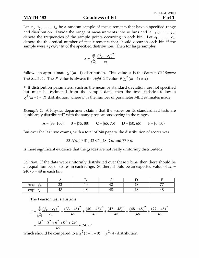
Dr. Neal, WKU MATH 482 Goodness of Fit Part 1 Let x1, x2 , . . . , xn be a random sample of measurements that have a specified range and distribution. Divide the range of measurements into m bins and let f1 , . . . , f m denote the frequencies of the sample points occurring in each bin. Let e1 , . . ., em denote the theoretical number of measurements that should occur in each bin if the sample were a perfect fit of the specified distribution. Then for large samples

x =( f k − ek )2

ekk =1

m∑

follows an approximate χ2(m −1) distribution. This value x is the Pearson Chi-Square Test Statistic. The P -value is always the right-tail value P(χ2 (m −1) ≥ x) . • If distribution parameters, such as the mean or standard deviation, are not specified but must be estimated from the sample data, then the test statistics follow a χ2 (m −1 − d) distribution, where d is the number of parameter MLE estimates made. Example 1. A Physics department claims that the scores on its standardized tests are “uniformly distributed” with the same proportions scoring in the ranges

A – [88, 100] B – [75, 88) C – [65, 75) D – [50, 65) F – [0, 50) But over the last two exams, with a total of 240 papers, the distribution of scores was

33 A's, 40 B's, 42 C's, 48 D's, and 77 F's. Is there significant evidence that the grades are not really uniformly distributed? Solution. If the data were uniformly distributed over these 5 bins, then there should be an equal number of scores in each range. So there should be an expected value of ek = 240/5 = 48 in each bin.

A B C D F freq: f k 33 40 42 48 77 exp: ek 48 48 48 48 48

The Pearson test statistic is

x = ( f k − ek )2

ekk=1

5∑ =

(33 − 48)2

48+(40 − 48)2

48+(42 − 48)2

48+(48 − 48)2

48+(77 − 48)2

48

=152 + 82 + 62 + 02 + 292

48≈ 24.29

which should be compared to a χ2 (5 − 1 − 0) = χ2 (4) distribution.

Dr. Neal, WKU If this data really were uniformly distributed as specified with the 5 ranges, then most test statistics would be near the “middle” of the χ2 (4) distribution, just like most normal measurements are within a standard deviation of average. If the data really were from a uniformly distributed, then there would be only a small chance of obtaining a large test statistic. But when there are large differences between what should occur ek and what did occur f k , then the test statistic will be large.

x

So for our test statistic x ≈ 24.29, we compute P χ2 (4) ≥ 24.29( ) , the right-tail probability that becomes the P -value. If the P -value is small (generally less than 0.10), then we have evidence to state that the data did not come from the stated distribution. Using the command χ 2cdf(24.29, 1E99, 4) , we obtain a P -value of about 0.00007. Thus we can say:

“If the grades really were uniformly distributed, then we would only have about 0.00007 probability of obtaining our frequencies f k from 240 grades that differ so much from the expected values ek in these 5 bins. This very low P -value gives us strong evidence to reject the claim that the grades are uniformly distributed as claimed.”

Example 2. Among Republicans, reported preferences for the 2016 Presidential election are:

Donald Trump Rand Paul Ted Cruz Ben Carson 35% 15% 30% 20%

However an independent poll of 900 Republicans gave the following preferences:

Donald Trump Rand Paul Ted Cruz Ben Carson

300 125 290 185 Does the survey poll give evidence to reject the reported preferences? Do a chi-square test of fit, give the P -value, and give a conclusion. Solution. If the reported preferences were correct, then the expected numbers of preferences for each candidate with a poll of 900 people would be

Trump Paul Cruz Carson ek = 900 × pct 315 135 270 180

We now have the actual frequencies f k and the expected results ek assuming the reported preferences were true:

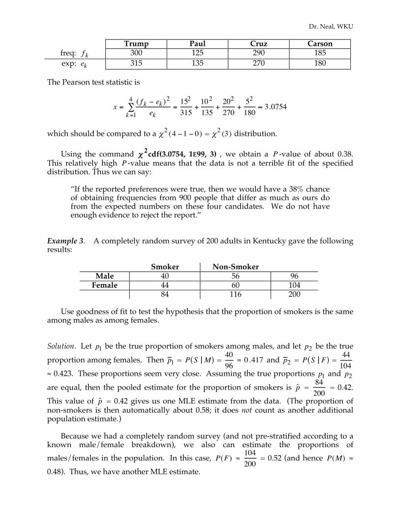
Dr. Neal, WKU Trump Paul Cruz Carson

freq: f k 300 125 290 185 exp: ek 315 135 270 180

The Pearson test statistic is

x =( f k − ek )2

ekk=1

4∑ =

152

315+102

135+202

270+52

180≈ 3.0754

which should be compared to a χ2 (4 −1 − 0) = χ2 (3) distribution. Using the command χ 2cdf(3.0754, 1E99, 3) , we obtain a P -value of about 0.38. This relatively high P -value means that the data is not a terrible fit of the specified distribution. Thus we can say:

“If the reported preferences were true, then we would have a 38% chance of obtaining frequencies from 900 people that differ as much as ours do from the expected numbers on these four candidates. We do not have enough evidence to reject the report.”

Example 3. A completely random survey of 200 adults in Kentucky gave the following results:

Smoker Non-Smoker Male 40 56 96

Female 44 60 104 84 116 200

Use goodness of fit to test the hypothesis that the proportion of smokers is the same among males as among females. Solution. Let p1 be the true proportion of smokers among males, and let p2 be the true

proportion among females. Then p 1 = P S M( ) = 4096

≈ 0.417 and p 2 = P S F( ) = 44104

≈ 0.423. These proportions seem very close. Assuming the true proportions p1 and p2

are equal, then the pooled estimate for the proportion of smokers is ˆ p = 84200

= 0.42.

This value of ˆ p = 0.42 gives us one MLE estimate from the data. (The proportion of non-smokers is then automatically about 0.58; it does not count as another additional population estimate.) Because we had a completely random survey (and not pre-stratified according to a known male/female breakdown), we also can estimate the proportions of males/females in the population. In this case, P(F) ≈ 104

200 = 0.52 (and hence P(M) ≈

0.48). Thus, we have another MLE estimate.

Dr. Neal, WKU Now if the true proportion of smokers were the same among males as among females, and is estimated to be about ˆ p = 0.42, then what results should we have expected in our survey?

Expected ek S N S N M 0.42× 96 0.58× 96 or M 40.32 55.68 F 0.42× 104 0.58× 104 F 43.68 60.32

Obtained f k

S N M 40 56 F 44 60

In each of the 4 bins, the difference between expected and actual is 0.32. So the Pearson test statistic is

x =( f k − ek )2

ek=

k=1

4∑

0.322

40.32+0.322

55.68+0.322

43.68+0.322

60.32= 0.00842 ,

which should be compared to a χ2 (4 −1 − 2) = χ2 (1) distribution (2 MLE estimates are used). Then using the command χ 2cdf(.00842, 1E99, 1) we obtain a P -value of about 0.926885. Because of the high P -value, the data is almost a perfect fit of the expected distribution given that the real proportion of smokers is 0.42.

Using the Two-Sided 2-Proportion Z-Test If we test H0 : p1 = p2 with a two-sided alternative Ha : p1 ≠ p2 , then we obtain the exact same P -value of 0.926885. In this case, the z test statistic is z = –0.0917643617.

But note that (−0.0917643617)2 = 0.00842, which is the exact value of the Pearson chi-square test statistic. However, by definition, Z2 = χ2(1) , when Z ~ N(0, 1) . So the goodness of fit test for two proportions is equivalent to the two-sided 2–Proportion Z test.

Dr. Neal, WKU

Poisson Fit Test

Many phenomena are modeled by a Poisson distribution, often because of empirical evidence, but sometimes just for mathematical simplification. The occurrences also can be distributed spatially, or otherwise, and not just measured during time intervals. Following are some examples of that show how to test whether data actually follows a Poisson distribution.

Example 4. In the bacterium E. coli, a mutant variety is resistant to the drug streptomycin. Do the occurrences of mutant resistant colonies follow a Poisson distribution? Experiment: 150 Petri dishes were plated with one million bacteria each. Below are the results on how many dishes formed each number of resistant colonies.

# of resistant

colonies

# of dishes 0 98 1 40 2 8 3 3 4 1

Does the data come from a Poisson distribution? If so, then what is the best estimate for λ ? For this λ , what would be the expected number of dishes ek forming each number of resistant colonies in the above table for k = 0, 1, 2, . . . ? Solution. Here we use the MLE estimate of the Poisson average λ , which is the sample average number of resistant colonies that formed. Thus, we have

ˆ λ =0 × 98 + 1 × 40 + 2 × 8 + 3 × 3 + 1 × 4

150 = 0.46.

Now if λ = 0.46, then for k = 0, 1, 2, 3, we have ek = 150 × 0. 46k e−0.46

k !. But for the

last bin, we use e4 = 150 × P(X ≥ 4) = 150 − e0 − e1 − e2 − e3 . We then have

# of resistant colonies

# of dishes

ek

0 98 94.693 1 40 43.559 2 8 10.018 3 3 1.5362

4 or more 1 0.1938 Does there appear to be a “significant” difference between what did occur and what should occur if the distribution really were Poi(0. 46)? We now test with the Pearson test statistic.

Dr. Neal, WKU We now have a test statistic of

x = ( f k − ek )2

ekk∑ = 3.307

2

94.693+3.5592

43.559+2. 0182

10.018+1.46382

1.5362+0.80622

0.1938≈ 5.56135 .

Since we have 5 bins and 1 MLE in use, we use a χ2 (5 − 1 −1) = χ2(3) curve to obtain a P -value of P(χ2 (3) ≥ 5.56135) ≈ 0.135 . If the data were from a Poi(0. 46) distribution, then we would have a 13.5% chance of obtaining frequencies from 150 observations that differ as much as ours do from expected in the 5 bin ranges. We do not have enough evidence to reject a Poi(0. 46) distribution.

Below we do the computations on a TI in order to have less round-off error:

Enter range

and frequencies 1–VarStats L1, L2

computes x ˆ λ = x = 0 .46 Store expected

into L3

Stat Edit

Must adjust last bin in L3 Edit L3(5) to

150 – 94.693 – 43.559 – etc Expected in L3

Compute error

terms in test stat Error terms in L4 Compute stats

on L4 The sum Σ x is the test stat

χ 2cdf (5. 561584885, 1E99, 3)

P-Value Note: The last bin contributes the most error to the test stat even though it has only one measurement. To avoid this problem, we could combine the last two bins as one bin and then use a χ2cdf(2) curve to compute the test stat.

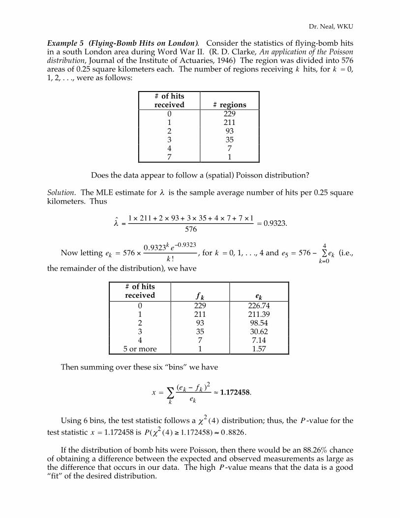
Dr. Neal, WKU Example 5 (Flying-Bomb Hits on London). Consider the statistics of flying-bomb hits in a south London area during Word War II. (R. D. Clarke, An application of the Poisson distribution, Journal of the Institute of Actuaries, 1946) The region was divided into 576 areas of 0.25 square kilometers each. The number of regions receiving k hits, for k = 0, 1, 2, . . ., were as follows:

# of hits received

# regions

0 229 1 211 2 93 3 35 4 7 7 1

Does the data appear to follow a (spatial) Poisson distribution?

Solution. The MLE estimate for λ is the sample average number of hits per 0.25 square kilometers. Thus

ˆ λ =1 × 211 + 2 × 93 + 3 × 35 + 4 × 7 + 7 ×1

576 = 0.9323.

Now letting ek = 576 × 0.9323k e−0.9323

k !, for k = 0, 1, . . ., 4 and e5 = 576 − ek

k=0

4∑ (i.e.,

the remainder of the distribution), we have

# of hits received

f k

ek

0 229 226.74 1 211 211.39 2 93 98.54 3 35 30.62 4 7 7.14

5 or more 1 1.57 Then summing over these six “bins” we have

x = (ek − f k )2

ekk∑ ≈ 1.172458.

Using 6 bins, the test statistic follows a χ2 (4) distribution; thus, the P -value for the test statistic x = 1.172458 is P(χ2 (4) ≥ 1.172458) ≈ 0.8826 . If the distribution of bomb hits were Poisson, then there would be an 88.26% chance of obtaining a difference between the expected and observed measurements as large as the difference that occurs in our data. The high P -value means that the data is a good “fit” of the desired distribution.

Dr. Neal, WKU

Enter range

and frequencies 1–VarStats L1, L2

computes x ˆ λ = x ≈ 0. 9323 Store expected

into L3

Stat Edit

Must adjust last bin in L3 Edit L3(5) to

576– 226.74– 211.39– etc Expected in L3

Compute error

terms in test stat Error terms in L4 Compute stats

on L4 The sum Σ x is the test stat

P-Value

Dr. Neal, WKU

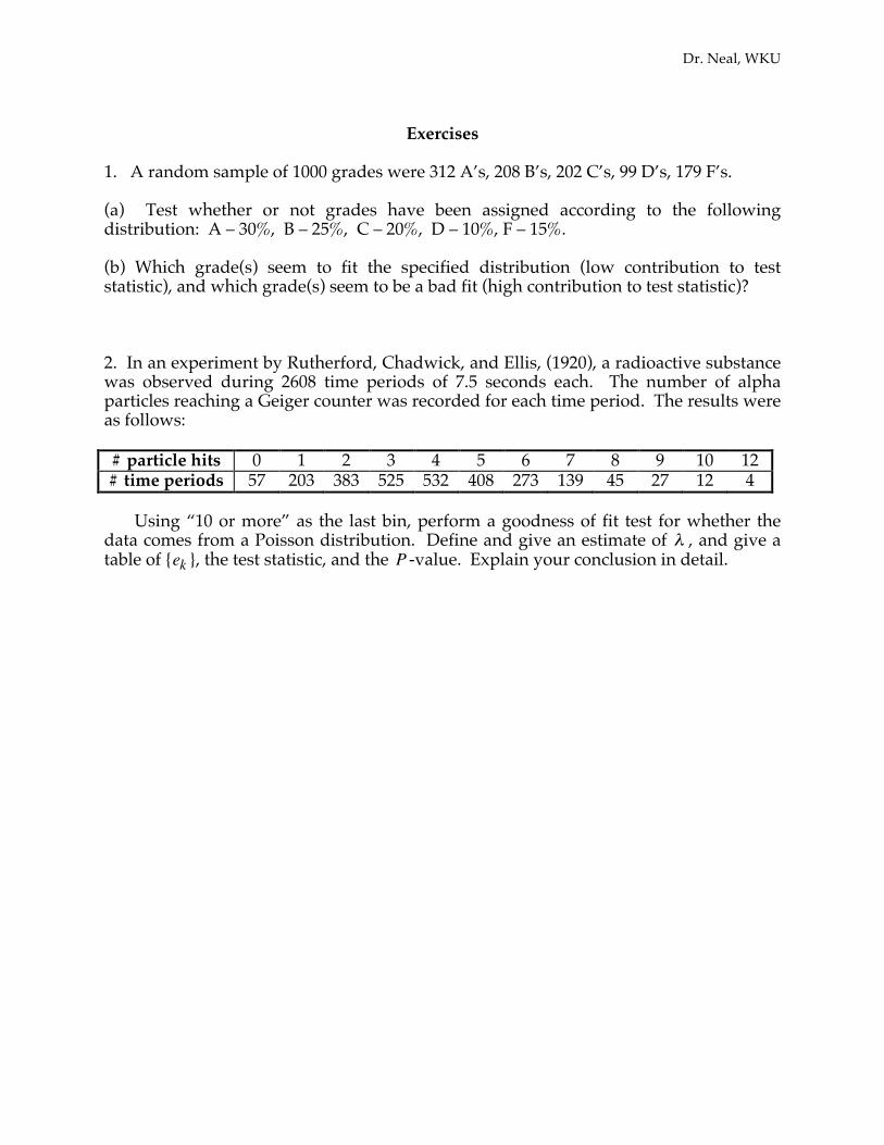
Exercises 1. A random sample of 1000 grades were 312 A’s, 208 B’s, 202 C’s, 99 D’s, 179 F’s. (a) Test whether or not grades have been assigned according to the following distribution: A – 30%, B – 25%, C – 20%, D – 10%, F – 15%. (b) Which grade(s) seem to fit the specified distribution (low contribution to test statistic), and which grade(s) seem to be a bad fit (high contribution to test statistic)? 2. In an experiment by Rutherford, Chadwick, and Ellis, (1920), a radioactive substance was observed during 2608 time periods of 7.5 seconds each. The number of alpha particles reaching a Geiger counter was recorded for each time period. The results were as follows: # particle hits 0 1 2 3 4 5 6 7 8 9 10 12 # time periods 57 203 383 525 532 408 273 139 45 27 12 4

Using “10 or more” as the last bin, perform a goodness of fit test for whether the data comes from a Poisson distribution. Define and give an estimate of λ , and give a table of {ek }, the test statistic, and the P -value. Explain your conclusion in detail.