December 16, 2005

To the Graduate School:

This thesis entitled “Motion Segmentation at Any Speed” andwritten by Shrinivas J.Pundlik is presented to the Graduate School of Clemson University. I recommend that itbe accepted in partial fulfillment of the requirements for the degree of Master of Sciencewith a major in Electrical Engineering.

Dr. Stanley Birchfield, Thesis Advisor

We have reviewed this thesisand recommend its acceptance:

Dr. Ian Walker

Dr. Adam Hoover

Accepted for the Graduate School:

MOTION SEGMENTATION AT ANY SPEED

A Thesis

Presented to

the Graduate School of

Clemson University

In Partial Fulfillment

of the Requirements for the Degree

Master of Science

Electrical Engineering

by

Shrinivas J. Pundlik

December 2005

Advisor: Dr. Stanley Birchfield

ABSTRACT

Common fate, or common motion, is a very strong cue for segmentation, and hence

motion segmentation is a widely studied problem in computervision. Most previous seg-

mentation approaches deal with motion either between two frames of the sequence or in the

entire spatio-temporal volume. In this thesis an incremental approach to motion segmenta-

tion is presented that allows for a variable number of image frames to affect the decision

process, thus enabling objects to be detected independently of their velocity in the image.

Feature points are detected and tracked throughout an imagesequence, and the features are

grouped using a region-growing algorithm with an affine motion model. The algorithm uses

a single parameter, which is the amount of evidence that mustaccumulate before features

are grouped. Procedures are presented for grouping features, measuring the consistency of

the resulting groups, assimilating new features into existing groups, and splitting groups

over time. Experimental results on a number of challenging image sequences demonstrate

the effectiveness of the technique.

DEDICATION

This thesis is dedicated to my mother and father who have always been supportive in

my endeavors.

ACKNOWLEDGEMENTS

I am indebted to my advisor, Dr. Stan Birchfield, for his guidance, encouragement and

support throughout the course of this work.

I would like to thank Dr. Ian Walker and Dr. Adam Hoover for agreeing to be part of

my thesis committee and for their helpful suggestions.

Finally, I would like to thank all my friends and lab mates whomade my stay at Clem-

son a memorable experience.

TABLE OF CONTENTS

Page

TITLE PAGE . . . . . . . . . . . . . . . . . . . . . . . . . . . . . . . . . . . . . . . . . .. . . . . . . . . . . . . . . . . . . . . . . . . . i

ABSTRACT . . . . . . . . . . . . . . . . . . . . . . . . . . . . . . . . . . . . . . . . . . .. . . . . . . . . . . . . . . . . . . . . . . . . . ii

DEDICATION . . . . . . . . . . . . . . . . . . . . . . . . . . . . . . . . . . . . . . . . .. . . . . . . . . . . . . . . . . . . . . . . . . . iii

ACKNOWLEDGEMENTS . . . . . . . . . . . . . . . . . . . . . . . . . . . . . . . . . . .. . . . . . . . . . . . . . . . . . . . iv

LIST OF FIGURES . . . . . . . . . . . . . . . . . . . . . . . . . . . . . . . . . . . . . .. . . . . . . . . . . . . . . . . . . . . . . . vii

CHAPTER

1. INTRODUCTION . . . . . . . . . . . . . . . . . . . . . . . . . . . . . . . . . . . . .. . . . . . . . . . . . . . . . . . . 1

Incremental Approach to Motion Segmentation . . . . . . . . . . . .. . . . . . . . . . . . . . . 3Previous Work . . . . . . . . . . . . . . . . . . . . . . . . . . . . . . . . . . . . . . .. . . . . . . . . . . . . . . . . . . 4Overview . . . . . . . . . . . . . . . . . . . . . . . . . . . . . . . . . . . . . . . . . . .. . . . . . . . . . . . . . . . . . . . 6Outline . . . . . . . . . . . . . . . . . . . . . . . . . . . . . . . . . . . . . . . . . . . .. . . . . . . . . . . . . . . . . . . . . 7

2. FEATURE TRACKING . . . . . . . . . . . . . . . . . . . . . . . . . . . . . . . . . .. . . . . . . . . . . . . . . . . 8

Motivation . . . . . . . . . . . . . . . . . . . . . . . . . . . . . . . . . . . . . . . . .. . . . . . . . . . . . . . . . . . . . . 8Feature Tracking Algorithm . . . . . . . . . . . . . . . . . . . . . . . . . . .. . . . . . . . . . . . . . . . . . 9Finding Good Features . . . . . . . . . . . . . . . . . . . . . . . . . . . . . . . .. . . . . . . . . . . . . . . . . . 9Limitations of the KLT Feature Tracker . . . . . . . . . . . . . . . . . .. . . . . . . . . . . . . . . . 12Affine Consistency Check . . . . . . . . . . . . . . . . . . . . . . . . . . . . . .. . . . . . . . . . . . . . . . . 12

3. FEATURING CLUSTERING . . . . . . . . . . . . . . . . . . . . . . . . . . . . . .. . . . . . . . . . . . . . . 14

Introduction to Clustering. . . . . . . . . . . . . . . . . . . . . . . . . . .. . . . . . . . . . . . . . . . . . . . . 14Feature Clustering Using K-means . . . . . . . . . . . . . . . . . . . . . .. . . . . . . . . . . . . . . . . 14Clustering Using an Affine Motion Model . . . . . . . . . . . . . . . . . .. . . . . . . . . . . . . . 18Clustering Using Normalized Cuts . . . . . . . . . . . . . . . . . . . . . .. . . . . . . . . . . . . . . . . 21

4. SEGMENTATION BY REGION GROWING . . . . . . . . . . . . . . . . . . . . . .. . . . . . . . 23

Grouping Features Using Two Frames . . . . . . . . . . . . . . . . . . . . .. . . . . . . . . . . . . . . 23Finding Neighbors . . . . . . . . . . . . . . . . . . . . . . . . . . . . . . . . . . .. . . . . . . . . . . . . . . . . . . 24

vi

Table of Contents (Continued)

Page

5. CONSISTENCY OF FEATURE GROUPS . . . . . . . . . . . . . . . . . . . . . . .. . . . . . . . . . 27

Finding Consistent Groups . . . . . . . . . . . . . . . . . . . . . . . . . . . .. . . . . . . . . . . . . . . . . . . 27Maintaining Feature Groups Over Time . . . . . . . . . . . . . . . . . . .. . . . . . . . . . . . . . . 28

6. EXPERIMENTAL RESULTS . . . . . . . . . . . . . . . . . . . . . . . . . . . . . .. . . . . . . . . . . . . . . 33

7. CONCLUSION . . . . . . . . . . . . . . . . . . . . . . . . . . . . . . . . . . . . . . .. . . . . . . . . . . . . . . . . . . . 39

BIBLIOGRAPHY . . . . . . . . . . . . . . . . . . . . . . . . . . . . . . . . . . . . . . .. . . . . . . . . . . . . . . . . . . . . . . . . 40

LIST OF FIGURES

Figure Page

1.1. Motion fields generated by sparse feature points distributed over theimage. LEFT: Motion between the first and the second frames of thesequence. RIGHT: Motion between first and the third frame. . . . . . . . . . . . . . . . 2

1.2. An object moves at constant speed against a stationary background.LEFT: If a fixed number of image frames are used, then slowly movingobjects are never detected. RIGHT: Using a variable number of imagesenables objects to be detected independently of their speed. . . . . . . . . . . . . . . . 3

2.1. Detection and tracking of features for real world sequences. Detectedfeatures overlaid on the first image and features tracked through thenth frame of the sequences.TOP: The statue sequence. BOTTOM: Thefreethrow sequence. . . . . . . . . . . . . . . . . . . . . . . . . . . . . . . . . .. . . . . . . . . . . . . . . . . . . . 11

2.2. Feature points obtained after the affine consistency check for the statuesequence. . . . . . . . . . . . . . . . . . . . . . . . . . . . . . . . . . . . . . . . . . .. . . . . . . . . . . . . . . . . . . . . 13

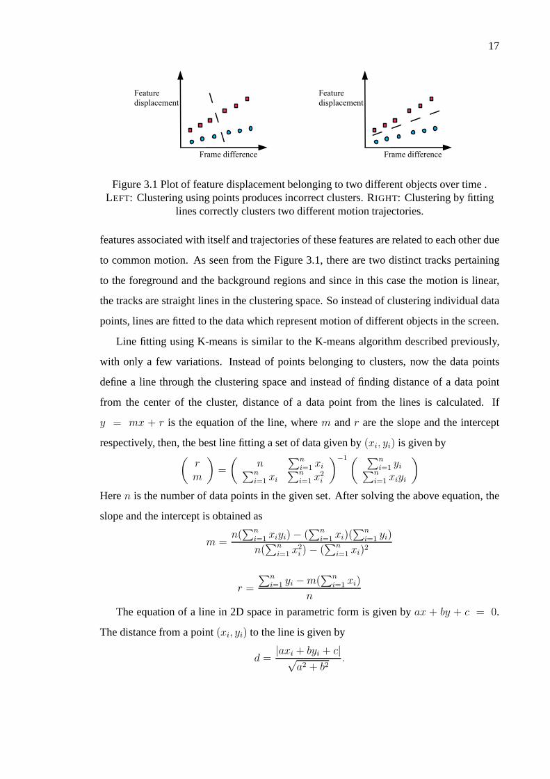
3.1. Plot of feature displacement belonging to two different objects over time. LEFT: Clustering using points produces incorrect clusters. RIGHT:Clustering by fitting lines correctly clusters two different motiontrajectories. . . . . . . . . . . . . . . . . . . . . . . . . . . . . . . . . . . . . . .. . . . . . . . . . . . . . . . . . . . . . . 17

3.2. TOP: Results of clustering of feature motion for flower-gardensequence(left) and Pepsi can sequence(right).BOTTOM: Motiontrajectories of the foreground and background regions in both thesequences .. . . . . . . . . . . . . . . . . . . . . . . . . . . . . . . . . . . . . . . . .. . . . . . . . . . . . . . . . . . . . . 19

3.3. Clustering feature motion using an affine motion model.LEFT: Theflowergarden sequence.RIGHT: The Pepsi can sequence. . . . . . . . . . . . . . . . . . . 19

3.4. Results of clustering using normalized cuts.LEFT: The flower-gardensequence with 2 clusters.CENTER: the flower-garden sequence 3clusters.RIGHT: The Pepsi-can sequence with 2 clusters . . . . . . . . . . . . . . . . .. 21

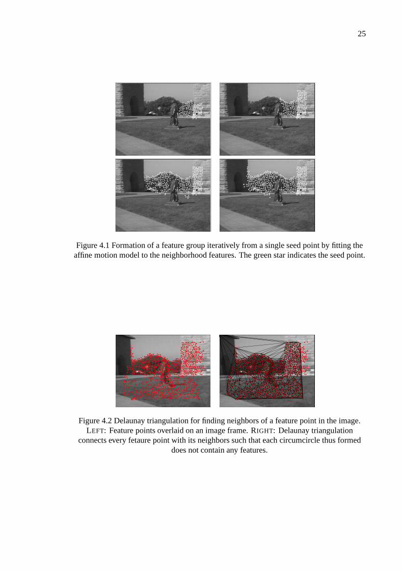
4.1. Formation of a feature group iteratively from a single seed point byfitting the affine motion model to the neighborhood features.The greenstar indicates the seed point. . . . . . . . . . . . . . . . . . . . . . . . . .. . . . . . . . . . . . . . . . . . . . 25

4.2. Delaunay triangulation for finding neighbors of a feature point in the

viii

List of Figures (Continued)

Figure Page

image. LEFT: Feature points overlaid on an image frame. RIGHT:Delaunay triangulation connects every fetaure point with its neighborssuch that each circumcircle thus formed does not contain anyfeatures. . . . . . 25

5.1. Results of region growing algorithm with different seed points for frames1 to 7 and grouping thresholdδg = 1.5. The consistent feature groups arethose which remain unchanged even if the seed points are changed andare shown in the last image (bottom-right). . . . . . . . . . . . . . .. . . . . . . . . . . . . . . . . 29

5.2. Addition of new features to existing feature groups. The squares and thetrinagles represent different feature groups with the arrows showing themotion of the features while the circles are the newly added features.The dotted lines represent the neighbors of the newly added features. . . . . . . 31

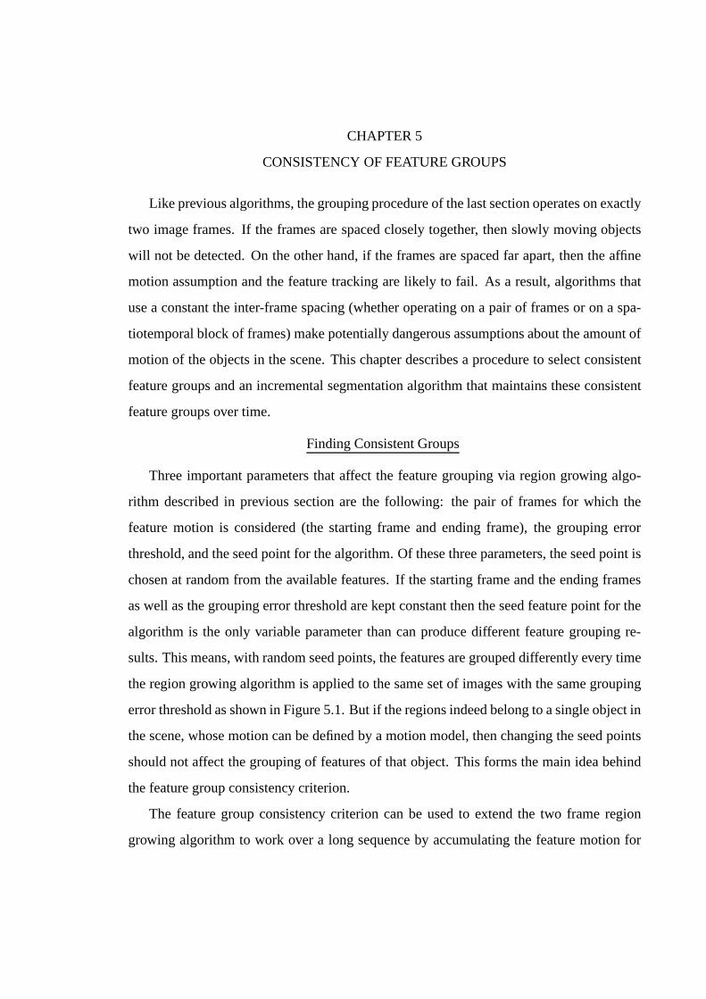
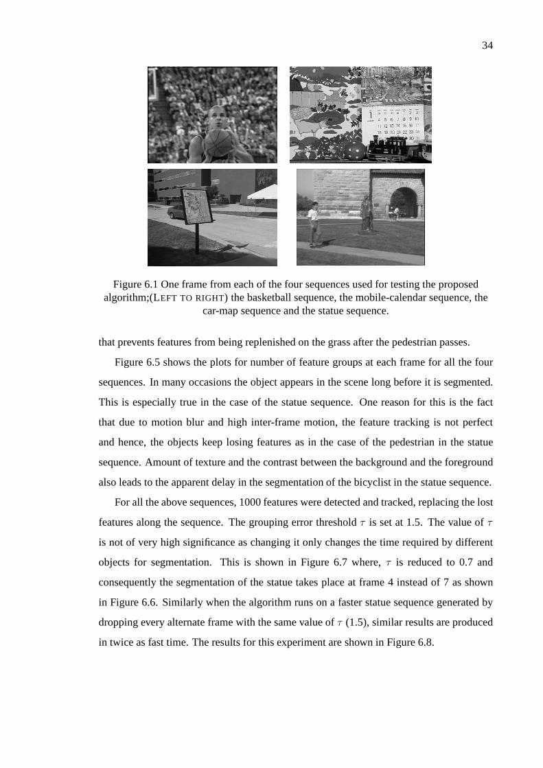
6.1. One frame from each of the four sequences used for testing theproposed algorithm;(LEFT TO RIGHT) the basketball sequence, themobile-calendar sequence, the car-map sequence and the statuesequence. . . . . . . . . . . . . . . . . . . . . . . . . . . . . . . . . . . . . . . . . . .. . . . . . . . . . . . . . . . . . . . . 34

6.2. Results of feature grouping algorithm on a 20 frame basketball sequence,with different group is shown by features of different colorand shape. . . . . . 35

6.3. Results of feature grouping algorithm on a 101 frame mobile-calendarsequence, with different group is shown by features of different colorand shape. . . . . . . . . . . . . . . . . . . . . . . . . . . . . . . . . . . . . . . . . . .. . . . . . . . . . . . . . . . . . . . 35

6.4. Results of feature grouping algorithm on car-map sequence, withdifferent group is shown by features of different color and shape. . . . . . . . . . . 36

6.5. The dynamic progress of the algorithm on the four sequences, plottedas the number of feature groups versus time. The number of groups isdetermined dynamically and automatically by the algorithm. . . . . . . . . . . . . . . 36

6.6. Results of feature grouping algorithm on a 520 frame statue sequence.The feature points in black in the first two frames are ‘ungrouped’. Afterthe first frame in which all of the features are ungrouped, subsequentimages show the formation of new groups or the splitting of existinggroups due to the arrival or departure of entities in the scene. . . . . . . . . . . . . . . 37

6.7. Results on the statue sequence withτ = 0.7. By reducing the thresholdby a factor of two, the segmentation occurs in nearly half thetime. . . . . . . . . . 38

ix

List of Figures (Continued)

Figure Page

6.8. Results of feature grouping algorithm on a 260 frame fast statuesequence generated by collecting every alternate frame from the originalsequence. The frame numbers below the figures correspond to those ofthe original statue sequence of Figure 6.6 . . . . . . . . . . . . . . .. . . . . . . . . . . . . . . . . . 38

CHAPTER 1

INTRODUCTION

An insight provided by the Gestalt psychology in the field of human visual perception

has led researchers to develop image and video segmentationsystems that delineate homo-

geneous image regions based on the Gestalt laws of grouping.The Gestalt theory of visual

perception argues that human visual perception is more adept at focusing on well-organized

patterns rather than on disparate parts, implying that grouping, or clustering, forms the fun-

damental idea behind visual interpretation. In the human visual system, representation of

an object is a result of grouping of individual neural responses, which in turn is guided by

factors underlying the scene such as similarity between theelements, closure, symmetry,

proximity, or common fate. These criteria for grouping are summarized as the Gestalt laws

of grouping.

An image can be effectively segmented using one or a combination of many different

criteria such as proximity, similarity, symmetry, or closure. For example, similarity of color

or intensity values of individual pixels can be used as one criteria of segmentation of an

image. At the same time, use of the proximity criteria rules out grouping together pixels or

regions of similar intensity far apart from each other in an image. Segmentation of videos is

a little more complicated process since videos are sequences of individual frames and time

becomes an important consideration. In such a situation, the criterion of common fate, or

common motion, is of special significance because it deals with the change in the scene

due to motion over time. Therefore, motion segmentation canbe defined as the grouping

or clustering of homogeneous image regions based on the criterion of similar motion.

Motion segmentation is important because it forms the basisof algorithms dealing with

object detection, tracking, surveillance, robot motion, image and video compression, and

shape recovery, among others. At the same time it is also a challenging task for variety

of reasons. First, the 3D motion in the scene is mapped to a 2D image plane making the

problem of quantifying image motion and subsequent recovery of the motion parameters an

under-constrained problem requiring additional constraints to be placed on the motion of

2

Figure 1.1 Motion fields generated by sparse feature points distributed over the image.LEFT: Motion between the first and the second frames of the sequence. RIGHT: Motion

between first and the third frame.

image regions. Image noise adds to the ambiguity to the motion parameters. For example,

noise may result in the change in the pixel values in subsequent frames even if there is no

motion between the two frames. Occlusions or disocclusionsmay occur in the sequence

when an object moves into the background, gets occluded by the foreground object and then

reappears into the foreground. This poses a challenge to accurate association of moving

regions through the sequence.

The two basic steps in a generic motion segmentation procedure are (1) determining

the motion vectors associated with each pixel assuming thatthe intensity of that pixel does

not change in the subsequent frames, and (2) clustering pixels that exhibit common mo-

tion. Instead of finding motion vectors associated with eachpixel, we can find key feature

points in the image and track those over the sequence to represent motion over an image

sequence. The resulting motion field looks similar to that generated using a dense optical

flow procedure (see Figure 1.1). Usually, motion field in an image refers to the true motion

of a pixel but in the present case it represents the motion of afeature point between two

frames. Grouping the features according to their motion is then equivalent to clustering

individual pixels and can be done in multiple ways, for example, by setting a global motion

threshold so that features with motion above the threshold value fall in one cluster and the

rest in another cluster, or by defining a threshold on the error in motion for a cluster of

features such that features with motion within the set errorrange are grouped together.

This thesis proposes an incremental approach toward motionsegmentation, where seg-

mentation of image regions is done when sufficient evidence has accumulated over time.

3

a b

Figure 1.2 An object moves at constant speed against a stationary background. LEFT: If afixed number of image frames are used, then slowly moving objects are never detected.

RIGHT: Using a variable number of images enables objects to be detected independentlyof their speed.

This is in contrast to most of the existing motion segmentation algorithms that process over

either two frames at a time or a spatio-temporal volume of a fixed number of frames as-

suming the motion of an object to be linearly changing or constant through the sequence.

Such algorithms fail to handle non-uniform motion of objects through the sequence. The

proposed approach enables motion segmentation over long sequences with multiple objects

in motion.

Incremental Approach to Motion Segmentation

One prominent challenge while grouping features is to reliably infer the velocities of

feature points of a sequence from the positions of the features in the corresponding image

frames due to tracking errors and image noise. A related problem is the accumulation of

sufficient evidence through the sequence to enable an accurate segmentation of the scene.

The evidence for segmentation in the present context is the motion of features in the se-

quence. Since the features associated with the objects in the scene may move with different

velocities, accumulation of evidence for segmentation mayrequire different number of

frames for different features at different instances of time. Accumulating an arbitrarily

large number of frames may not guarantee a reliable solutionas the feature tracks may vary

unpredictably through the sequence.

Traditional approaches toward motion segmentation have been to consider image mo-

tion between two frames of a sequence at a time and perform motion segmentation by

setting a threshold on the velocities of the regions (see Figure 1.2a). If a region is moving

4

with a velocity less than the threshold then it may never be detected. An alternative is to set

a fixed threshold on the displacement of the image regions. The advantage of this approach

is that if we wait for a sufficient time then regions moving with a very small velocity can

be also detected (see Figure 1.2b). So in such a situation thesegmentation is related to

the process of accumulating evidence of motion. While considering image motion in two

frames, instead of segmenting the whole scene, we wait untilwe have sufficient evidence

to segment each region. As a result, different objects are segmented from the scene over a

period of time depending upon their motion in the image with respect to the same reference

frame. Once the initial segmentation is achieved over a period of time, the individual image

regions are tracked and their motion models are updated while including the new informa-

tion that appears in the scene. This addresses the problem ofsuccessfully segmenting long

image sequences with multiple image regions in non-uniformmotion.

Previous Work

Different techniques exist to quantify the image motion andperform motion segmen-

tation based on such a measure. There are two approaches for motion segmentation. One

relies on the low level image data to find the motion of each pixel and then tries to combine

this information to come up with some kind of estimate of image motion as a whole. This

is termed as a bottom-up approach in the field of computer vision. The other approach,

which is known as a top down approach, tries to label different image regions in motion

using some a priori information or some high level model.

Some of the earlier approaches use optical flow fields to describe the 2D velocity of

the pixels of the image. A smoothness constraint is imposed on the velocities of the neigh-

boring pixels. This kind of approach is fraught with the problems like dealing with large

untextured areas in an image or effective imposition of the smoothness constraint so as to

not smooth over the discontinuities.

More recent approaches allow simultaneous estimation of multiple global motion mod-

els with a layered representation of the image [15], [1], [16], [17], [19], [18], [9]. Earliest of

such approaches was proposed by Wang and Adelson [15]. They estimate the optical flow

and group pixels using an affine motion model iteratively such that a model corresponding

5

to each layer in the sequence is obtained. Subsequent paperson the layered motion model

by Weiss [16], Weiss and Adelson [17] assume a set of parametric motion fields exist in the

motion sequence, each represented by a probabilistic modelwhile the overall motion in the

sequence is given by a mixture model. To find motion at an individual pixel, a particular

motion field set is determined and a sample is drawn from it. Inthis case both, the parame-

ter values of the motion field and the motion field associated with each pixel are unknown.

This is a missing data problem and the expectation maximization (EM) algorithm is used

to iteratively determine the motion field an individual pixel belongs to and the parameters

of those motion fields [6]. Layer based motion segmentation using graph cuts is described

in Xiao and Shaah [19], Wills et. al. [18] while Ke and Kanade [9] use a subspace based

approach, originally proposed in [5], to assign pixels to different layers. Layered motion

model approach of motion segmentation are effective in demarcating the motion bound-

aries and allow reconstructing the motion sequence by manipulating the individual motion

layers. Limitation of this approach lies in the initialization phase, where one has to decide

beforehand the nature of the motion models. Motion segmentation using multiple cues

such as color, spatial relationships and motion is discussed in [10].

A fundamentally different approach based on normalized cuts algorithm was proposed

by Shi and Malik [13]. The motion segmentation is posed as a graph partitioning problem

in a spatio-temporal volume and solved as a generalized eigenvalue problem. A weighted

graph is constructed with each pixel as a node connected to pixels in the spatio-temporal

neighborhood and segmented using the normalized cuts algorithm. The normalized cuts

framework splits the weighted graph constructed earlier ina balanced manner instead of

splitting small isolated regions. The normalized cuts algorithm outputs a matrix containing

the weights for association of each node to the different clusters. The approach is compu-

tationally expensive.

Image motion leads to such interesting phenomena as motion discontinuities and oc-

clusion boundaries in the image. Different image patches moving with different velocities

give rise to motion discontinuities as some image regions may move in front of others,

occluding them. The boundary of the foreground region formsthe occlusion boundary be-

tween it and the occluded region. These motion discontinuities or occlusion boundaries

6

through a sequence can lead to reliable motion segmentationof the scene. Black and Fleet

[4] describe an algorithm for detection and tracking of motion discontinuities using the

condensation algorithm which is extended in [11] by incorporating edge information along

with the motion information for better motion boundary localization.

As an alternative to dense optical flow, motion between two frames of a image sequence

can be represented by detecting and tracking point featuresbetween the frames. The fea-

tures are small image regions that exhibit high intensity variation in more than one direction

[14]. Some work [2],[8] involves detecting and tracking such point features and grouping

them based on motion in case of vehicle tracking scenario. Segmentation and tracking of

human limb motion using robust feature tracks is described in [7]. Approach described in

[3] finds good features in the sequence and groups them iteratively using an affine motion

model.

Overview

The work presented in this thesis is based on the algorithm proposed by Birchfield [3]

for detecting motion discontinuities between two frames ofa sequence. Point features are

detected and tracked through the sequence and motion between two frames is considered to

group the point features according to an affine motion model to find different image regions

in motion. Using this two frame motion segmentation algorithm, segmentation of the whole

scene is done incrementally, over a period of time. The evidence of segmentation is calcu-

lated by a feature group consistency criterion that measures the consistency, or similarity,

of feature groups formed under varying conditions. Motion models are computed for each

of the feature groups and the groups are tracked through the sequence while continuously

updating the motion model to accommodate scene changes occurring over time.

To summarize, this thesis describes:

1. various methods for grouping features based on their motion in two frames of a se-

quence,

2. different parameters that affect the feature grouping process, and

3. an algorithm to extend the two frame motion segmentation algorithm to work with

multiple frames.

7

Outline

The rest of the text is organized as follows. In Chapter 2 detection and tracking of fea-

tures in a video sequence is described. Two different methods of feature grouping namely,

clustering and region growing are explained in Chapter 3 andChapter 4 respectively. In

Chapter 5, the feature group consistency criterion and maintenance of the feature group is

described. Experimental results on variety of image sequences are demonstrated in Chapter

6. Finally, conclusions and future work are presented in Chapter 7.

CHAPTER 2

FEATURE TRACKING

Any algorithm dealing with motion segmentation has to tackle the problem of quan-

tifying the image motion. An ideal measure of image motion accurately identifies image

regions undergoing different motion in varying circumstances. This means, it allows effi-

cient recovery of the motion parameters and helps in establishing correspondence between

the subsequent frames in an image sequence. It builds the motion hypothesis based on the

low level operators, i.e., it follows a bottom-up approach.This makes it general enough to

be applied to different kinds of images in different circumstances. Point features, though

not an ideal measure, are sufficient to represent image motion in this thesis. This chapter

describes the motivation behind selecting point features for motion representation, the al-

gorithm to detect and track the features through an image sequence and its limitations. It

further describes a method to improve the performance of thefeature tracking algorithm

while dealing with a long sequence.

Motivation

There are two principal ways to represent image motion. One approach is to use dense

motion fields, i.e., to find motion vectors associated with each pixel in an image while

the other approach is to detect key feature points in the image and find motion vector of

each feature point. The main motivation behind using sparsefeature points spread over the

image instead of a dense motion field representation is to reduce the time and complexity

of the computation. Since in most cases the image regions under motion are much larger

than a pixel, a dense motion field has a lot of redundant information. The same information

can be reliably obtained from a large number of features spread over the image with less

computational cost. For example in the experiments described in this thesis, 1000 features

are enough to cover an image of size320× 240 instead of 76,800 motion vectors.

Feature points are not individual pixels but a neighborhoodof pixels taken together.

They capture the intensity variation in this neighborhood and are reliable low-level oper-

9

ators making them repeatable under varying circumstances (for example, between subse-

quent frames of an image sequence). Also, establishing correspondence between features

in two frames becomes easy and for this reason they are well suited for the process of

tracking. Since they consider a neighborhood of pixels, theeffect of noise is reduced. To

summarize, motion of feature points through the sequence gives an effective representation

of image motion and hence, detecting and tracking feature points forms the very basis of

the proposed motion segmentation algorithm.

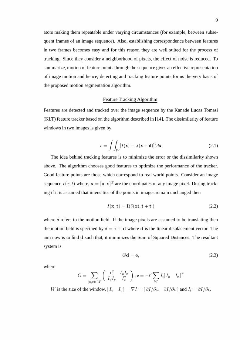
Feature Tracking Algorithm

Features are detected and tracked over the image sequence bythe Kanade Lucas Tomasi

(KLT) feature tracker based on the algorithm described in [14]. The dissimilarity of feature

windows in two images is given by

ǫ =

∫ ∫

W

[I(x)− J(x + d)]2dx (2.1)

The idea behind tracking features is to minimize the error orthe dissimilarity shown

above. The algorithm chooses good features to optimize the performance of the tracker.

Good feature points are those which correspond to real worldpoints. Consider an image

sequenceI(x, t) where,x = [u,v]T are the coordinates of any image pixel. During track-

ing if it is assumed that intensities of the points in images remain unchanged then

I(x, t) = I(δ(x), t + t′) (2.2)

whereδ refers to the motion field. If the image pixels are assumed to be translating then

the motion field is specified byδ = x + d whered is the linear displacement vector. The

aim now is to findd such that, it minimizes the Sum of Squared Distances. The resultant

system is

Gd = e, (2.3)

where

G =∑

(u,v)∈W

(

I2u IuIv

IuIv I2v

)

, e = −t′∑

W

It[ Iu Iv ]T

W is the size of the window,[ Iu Iv ] = ∇I = [ ∂I/∂u ∂I/∂v ] andIt = ∂I/∂t.

10

Finding Good Features

The matrix G in 2.3 is given by

G =

∫ ∫

W

(∇I)(∇I)T w(x)dx (2.4)

For a given image, the first step is to find the gradient for every coordinate point (i.e.,

each pixel). But individual pixels are not of any use for tracking over a sequence. Hence,

collection of pixels called feature window are tracked. Neighborhood pixels combine to

form a feature window. Integrating over this feature windowgives us a matrix G, whose

eigenvalues are of primary interest. Corresponding eigenvectors give the principal com-

ponents (direction) while the eigenvalues decide the amount of scaling of these vectors in

their respective directions. Since the G matrix consists ofspatial gradient information, its

eigenvectors and eigenvalues give the principal directionof change in the intensity and the

amount of change respectively. In general, a good feature isone which has its smallest

eigenvalue greater than the user defined threshold. Ifλ1 andλ2 are two eigenvalues of

G for a feature window such thatλ1 > λ2 andδfeat is the user defined threshold on the

eigenvalue, then feature is considered a good feature ifλ2 > δfeat.

Significance of having two large eigenvalues for the G matrixof a feature window is that

it shows the variation of intensities in more than one direction in the feature window. Such

locations in an image are important as they are the easiest tosearch in the subsequent frames

if their motion could be estimated. If bothλ1 andλ2 are below the thresholdδfeat, then

the feature window has uniform intensity and does not carry any significant information

which could identify the feature. As a result, texture-lessregions in an image do not have

any good features. This can be seen form Figure 2.1 (top row),where good features are not

detected in the clear sky. If one of the eigenvalues is very large as compared to the other

then it indicates a strong gradient in one direction, i.e., presence of an edge. Such a feature

window is not considered good as the location of the feature becomes ambiguous in the

subsequent frames.

As a result of feature tracking step, tracks of the feature points are obtained over the

required number of images. The detected features in the initial frame are shown in Figure

2.1 for two different sequences. Figure 2.1 (top-right and bottom-right) shows the features

11

Figure 2.1 Detection and tracking of features for real worldsequences. Detected featuresoverlaid on the first image and features tracked through the nth frame of thesequences.TOP: The statue sequence. BOTTOM: The freethrow sequence.

12

tracked from the initial frame through the final frame. As it can be seen some features are

lost while some new features are added as new scene appearersin the sequence.

Limitations of the KLT Feature Tracker

Certain assumptions made while developing the original KLTalgorithm limit the per-

formance of the feature tracker. KLT matches images in successive frames. This makes the

implementation easier but any feature information in previous frames is ignored. It cannot

model complex variations in the image region over a long sequence as this information

cannot be obtained only from displacement parameters.

It also assumes that there is no occlusion of the feature window in the next frame. Any

occlusion results in the loss of that feature altogether. Even if the feature reappears after a

few frames, there is nothing to establish correspondence between the lost and reappeared

feature. There also exists a problem about features straddling a depth discontinuity or

a boundary making such features unreliable for tracking. But still, depth discontinuities

and boundaries have wealth of information regarding the object being tracked, which KLT

cannot effectively utilize. Size of the tracking window plays an important role. If the

size of feature window is increased, then the motion variation information can be reliably

calculated but the risk of the feature drifting along with a boundary becomes more.

KLT considers each feature as an independent entity while tracking but in may situa-

tions the features may follow some pattern where they are notindependent. There are other

issues such as KLT assuming constant intensity levels over the successive frames and a

simple (rigid) geometry while calculating the transformations. Its performance deteriorates

when some image regions undergo non-rigid transformation.

Affine Consistency Check

In the feature tracking algorithm described above, the displacementd is calculated us-

ing a translational model and dissimilarity between a feature window in successive frames

is given by equation 2.1. While dealing with long image sequences, a feature window may

undergo significant changes and its appearance may become different as compared to its

original form in the frame in which it was detected. This leads to tracking failures such as

13

Figure 2.2 Feature points obtained after the affine consistency check for the statuesequence.

features straddling discontinuities or bunching of features near occlusion boundaries. This

effect can be seen in Figure 2.1 (top-right) where features are bunched together on the right

side of the statue.

Shi and Tomasi [14] describe an approach that measures the dissimilarity between a

feature in the current frame and the corresponding feature in the first frame by using an

affine motion model. Equation 2.1 can be modified to include the affine parameters as

ǫ =

∫ ∫

W

[I(x)− J(Ax + d)]2dx

which yields a system of linear equations pertaining to the six affine parameters solving for

which gives the distortion of the feature. Features are tracked in successive frames using

a translational model while comparison of features in the current frame and initial frame

is done using the affine model. If the dissimilarity exceeds the threshold value then the

feature is discarded. Feature tracking using affine consistency check is shown in Figure

2.2 and it can be seen that the features are evenly distributed and there is no bunching of

features at the motion discontinuities. This is incorporated in the latest version of KLT.

CHAPTER 3

FEATURING CLUSTERING

Once features are detected and tracked, the next step is to group all the features exhibit-

ing similar motion. This chapter describes some common clustering algorithms such as

K-means and normalized cuts for clustering features. Although the clustering techniques

are successful in grouping features in some simple image sequences, they have limitations

while handling long sequences. This chapter is just an exploration of various ideas and the

techniques described in it are subsumed by the next two chapters.

Introduction to Clustering

Clustering can be defined as the process of partitioning or segregation of a data set into

smaller subsets or clusters in a manner such that the elements of individual clusters share a

predefined similarity criterion. For images, in most cases the data set for clustering consists

of individual pixel values or vectors representing the color, coordinates of the pixels, the

texture around the pixel, or some other properties calculated from the image data. For a

typical clustering method, a data setX with its elements given byxi, is partitioned intoN

clustersC1,C2, . . . ,CN with meansµ1,µ2, . . . ,µN . Then an error measure that represents

how well the data is clustered can be defined using least squares:

e =

N∑

k=1

∑

xi∈Ck

‖ xi − µk ‖2 (3.1)

In many implementations of clustering techniques, the number of clustersN to be found

for a particular data set, is known beforehand. This enablesthe user to define an objective

function that can be optimized to obtain better clustering results. IfN is not known, then the

optimal number of clusters required can be found out from thepartitioning of the data itself

for example by setting a threshold on the variance of each cluster. Different techniques for

data clustering exist such as, K-means, agglomerative and divisive clustering, histogram

mode seeking, graph theoretic and so on.

15

Feature Clustering Using K-means

K-means is a very commonly used technique for data clustering. Before the clustering pro-

cess starts, the algorithm requires a prior knowledge of theclustering space and the number

of clusters to partition the data in. Usually, the clustering space depends on the dimension-

ality of the data elements. For images it may be a 1D space if only the pixel intensities are

used for classification, 2D if pixel coordinates are used or of multiple dimensional space if

each pixel is associated with a high dimensional vector describing local texture.

A simple form of K-means algorithm to cluster points in a 2D plane is discussed be-

low. It involves minimizing an objective function which is similar to the error measure for

clustering as shown in 3.1. A direct search for the minimum ofsuch a objective function is

not feasible as number of points may be large. Hence to tacklethis situation, the algorithm

iterates through two steps: assuming the cluster means, perform the allocations of the data

points and based on the point allocations in the previous steps, calculate the cluster means

till convergence. Convergence is achieved when the error value defined in 3.1 reaches be-

low a set threshold. Limitations of this algorithm are that it does not usually converge to a

global minimum and may not result inN clusters if zero elements are allocated to some of

the clusters initially. Still, the algorithm is easy to implement and is effective if the data to

be clustered is well separated. The complete algorithm is asfollows:

1. Choose the number of clustersN and randomly chooseN center points for these

clusters.

2. Allocate each data element to the cluster whose center is nearest to the data element(

for a 2D space the distance measure is Euclidean distance).

3. Update the clusters centers by finding the means of elements in each cluster.

4. Repeat steps 2 and 3 till the cluster centers do not change between two successive

iterations.

Small variations can be made in the algorithm described above while implementation

without changing the results in any significant way such as assigning the data points ran-

16

domly to the clusters initially and finding their means or changing the convergence condi-

tion in step 4.

Clustering Space

First step in clustering feature points based on common motion is to define a clustering

space that enables meaningful clustering of features. Consider two framesI1 andI2 of the

sequence shown in Figure 1.2. Let the number of features tracked from frameI1 to I2 ben.

If the position of a featurei in frameI1 is (xi, yi), then its position in frameI2 is given by

(xi + dxi, yi + dyi), wheredxi anddyi is the distance moved by the feature in thex andy

direction respectively. The total distance moved by the featurei in two frames is given by

di =√

dx2i + dy2

i .

The clustering space is defined by the total displacement of the features and the frame

difference, then for a pair of frames, the clustering space is unidimensional and the data set

is given by[d1, d2, . . . , dn]T . If the motion is present predominantly in one direction(asin

the case of Figure 1.2 where motion is only in the horizontal direction), then the data set

can be represented as[dx1, dx2, . . . , dxn]T .

For the reasons described in Chapter , motion computed by considering only two suc-

cessive frames may not be sufficient for correct segmentation of scene and hence, multiple

frames need to be considered. Now, the clustering space becomes a 2D space such that

each data point is represented byDi = [di k]T , wherei = 1, . . . , n are the features and

k = 1, . . . , F are the frames. The distance between each data pointDi in the clustering

space is measured as the Euclidean distance.

Fitting Lines

Considering each pointDi separate while clustering is valid only if the displacementis

calculated by considering only two frames i.e., for a 1D clustering space. When multiple

frames are considered then the each data pointDi associated with a feature cannot be

considered as a separate or distinct from the rest of the datapoints in a 2D clustering

space. If clustering is performed with this assumption, then the results are not accurate as

shown in Figure 3.1. This is because each object moving through the sequence has some

17

Figure 3.1 Plot of feature displacement belonging to two different objects over time .LEFT: Clustering using points produces incorrect clusters. RIGHT: Clustering by fitting

lines correctly clusters two different motion trajectories.

features associated with itself and trajectories of these features are related to each other due

to common motion. As seen from the Figure 3.1, there are two distinct tracks pertaining

to the foreground and the background regions and since in this case the motion is linear,

the tracks are straight lines in the clustering space. So instead of clustering individual data

points, lines are fitted to the data which represent motion ofdifferent objects in the screen.

Line fitting using K-means is similar to the K-means algorithm described previously,

with only a few variations. Instead of points belonging to clusters, now the data points

define a line through the clustering space and instead of finding distance of a data point

from the center of the cluster, distance of a data point from the lines is calculated. If

y = mx + r is the equation of the line, wherem andr are the slope and the intercept

respectively, then, the best line fitting a set of data given by (xi, yi) is given by(

rm

)

=

(

n∑n

i=1 xi∑n

i=1 xi

∑n

i=1 x2i

)

−1 (∑n

i=1 yi∑n

i=1 xiyi

)

Heren is the number of data points in the given set. After solving the above equation, the

slope and the intercept is obtained as

m =n(

∑n

i=1 xiyi)− (∑n

i=1 xi)(∑n

i=1 yi)

n(∑n

i=1 x2i )− (

∑n

i=1 xi)2

r =

∑n

i=1 yi −m(∑n

i=1 xi)

n

The equation of a line in 2D space in parametric form is given by ax + by + c = 0.

The distance from a point(xi, yi) to the line is given by

d =|axi + byi + c|√

a2 + b2.

18

If the slope is given bym = − ab

and the intercept isr = − cb, then the distance of a

point (xi, yi) to the line is given by

d =| −mxi + yi − r|√

m2 + 1.

The K-means algorithm, modified to fit lines to the given data is described below:

1. Choose the number of linesN and randomly chooseN set of parameters (slope and

intercept) for these lines.

2. Allocate each data element to the line closest to the data element.

3. Update the line parameters using the all points fitted by the line forN lines.

4. Repeat steps 2 and 3 till the line parameters do not change between two successive

iterations.

Results of clustering by using the above modified K-means algorithm are shown in

Figure 3.2. It can be seen from the plots of feature displacement with respect to frame

difference that features belonging to the foreground regions have a lot of variations in the

motion which leads to errors in clustering.

Clustering Using an Affine Motion Model

Clustering features in previous sections assumes a translational motion of the features.

This assumption is well suited for sequences where there is linear motion of the objects

(undergoing translation and rotations but no out of plane rotation) in the foreground such

as in the Pepsi can sequence. Image motion can be modeled in a more realistic manner

by using an affine motion model, that accounts for scaling andshear in addition to the

translation and rotation.

The affine partitioning algorithm partitions the given datainto distinct groups that ad-

here to affine motion models with different parameters. The data in the present context

refers to the feature motion in the affine space. Let the totalnumber of features ben and

N be the labels associated with different affine models according to which the features are

19

1 1.5 2 2.5 3 3.5 4 4.5 5−5

0

5

10

15

20

25

30

frame difference

feat

ure

disp

lace

men

t

features belonging to the tree

features belonging to the background

1 1.5 2 2.5 3 3.5 4 4.5 50

1

2

3

4

5

6

7

8

frame differencefe

atur

e ds

ipla

cem

ent

features belonging to the pesi can

features belonging to the background

Figure 3.2TOP: Results of clustering of feature motion for flower-garden sequence(left)and Pepsi can sequence(right).BOTTOM: Motion trajectories of the foreground and

background regions in both the sequences .

Figure 3.3 Clustering feature motion using an affine motion model. LEFT: Theflowergarden sequence.RIGHT: The Pepsi can sequence.

20

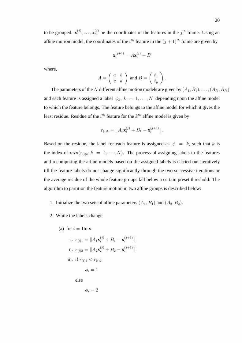
to be grouped.x(j)1 , . . . , x(j)

n be the coordinates of the features in thejth frame. Using an

affine morion model, the coordinates of theith feature in the(j + 1)th frame are given by

x(j+1)i = Ax(j)

i + B

where,

A =

(

a bc d

)

andB =

(

txty

)

.

The parameters of theN different affine motion models are given by(A1, B1), . . . , (AN , BN)

and each feature is assigned a labelφk, k = 1, . . . , N depending upon the affine model

to which the feature belongs. The feature belongs to the affine model for which it gives the

least residue. Residue of theith feature for thekth affine model is given by

r(i)k = ‖Akx(j)i + Bk − x(j+1)

i ‖.

Based on the residue, the label for each feature is assigned as φ = k, such thatk is

the index ofmin(r(i)k; k = 1, . . . , N). The process of assigning labels to the features

and recomputing the affine models based on the assigned labels is carried out iteratively

till the feature labels do not change significantly through the two successive iterations or

the average residue of the whole feature groups fall below a certain preset threshold. The

algorithm to partition the feature motion in two affine groups is described below:

1. Initialize the two sets of affine parameters(A1, B1) and(A2, B2).

2. While the labels change

(a) for i = 1to n

i. r(i)1 = ‖A1x(j)i + B1 − x(j+1)

i ‖

ii. r(i)2 = ‖A2x(j)i + B2 − x(j+1)

i ‖

iii. if r(i)1 < r(i)2

φi = 1

else

φi = 2

21

(b) Recompute(A1, B1) and(A2, B2) using least squares.

The clustering using affine motion model is shown in Figure 3.3. It can be noted that

the tree and the Pepsi can are segmented in a better manner as compared to clustering using

just translation of features(see Figure 3.2).

Clustering Using Normalized Cuts

Figure 3.4 Results of clustering using normalized cuts.LEFT: The flower-garden sequencewith 2 clusters.CENTER: the flower-garden sequence 3 clusters.RIGHT: The Pepsi-can

sequence with 2 clusters

Normalized cuts algorithm proposed in [12] views the segmentation as a graph parti-

tioning problem. LetG = (V, E) be the graph whose nodes are the points to be clustered

and letw(i, j) be the weight of the edge between nodesi andj representing the similarity

between the nodes. The objective is to partition the graph into m sets of nodes.

A cut is defined as the sum of weights of the edges that are removed while partitioning

the graph into two parts. For partitioning the graphG = (V, E) into sets of nodesA and

B, the cut is given by

cut(A, B) =∑

u∈a,v∈B

w(u, v)

Minimizing thecut(A, B) may produce the desired setsA andB but in many cases apply-

ing minimum cut is not a feasible idea because it leads to cutting of small isolated nodes.

The normalized cuts algorithm, normalizes the cut so as to produce an optimum partition

that is not biased in favor of cutting small parts of the graph. Normalized cuts, or Ncuts,

is defined in terms ofcut andassociation. Association of a region with the whole set of

nodes is defined as the sum of weights of the edges between the nodes in the region and all

the nodes in the graph. Hence, association of regionA with the complete setV is given by

asso(A, V ) =∑

u∈A,t∈V

w(u, t)

22

The normalized cut for a graph is given by

Ncut(A, B) =cut(A, B)

asso(A, V )+

cut(A, B)

asso(B, V )

If there areN nodes in the graph then aN dimensional vectord is defined such that

d(i) =

N∑

j=1

w(i, j)

where,i andj are the nodes of the graph. In present case, the nodes are the tracked features

in the image, the edge weightw(i, j) is the feature motion between two frames andd(i)

gives the similarity between the motion ofith feature and all the other features. AnN ×N

diagonal matrixD is defined withd on its diagonal, while anotherN × N symmetrical

matrix W is constructed such thatW (i, j) = w(i, j). Let x be theN partitioning vector

that indicates whether a node belongs to the setA or setB ans is given by

x =

{

1 if nodei is in A;−1 otherwise.

Finding a vectorx that shows the partitions of the nodes is a NP Hard problem and

hence, Ncuts solves the problem in continuous domain. A continuous approximation ofx

is given by

y = (1 + x)−∑

xi>0 di∑

xi<0 di

(1− x)

The eigenvector associated with the second smallest eigenvalue of the system

(D −W )y = λDy

outputs the optimum partition of the graph. To further sub-divide the two sets, the Ncuts

algorithm is applied to the set of nodes till the value of the cut is below a pre-specified

threshold. The results of using normalized cuts algorithm for clustering feature motion on

two sequences are shown in Figure 3.4. The algorithm is sensitive to the cut threshold and

a small variation in the threshold may produce significantlydifferent results.

CHAPTER 4

SEGMENTATION BY REGION GROWING

This chapter describes a region growing algorithm to group features based on their mo-

tion in two frames. The feature grouping algorithm presented in this chapter approaches

the problem from a different point of view as compared to the one described in Section ,

such that instead of starting with all the features as a single cluster of data and dividing it,

individual features are grouped together and the group is grown progressively. The prin-

cipal idea behind both the approaches remains the same, i.e., formation of feature groups

based on the motion of features. The next chapter describes methods to use the algorithm

presented here as the basis to perform motion segmentation over multiple frames.

Grouping Features Using Two Frames

Once features are tracked from one image frame to another, the features are grouped using

an affine motion model on the displacements of the coordinates of the features. In other

words, whether a featuref is incorporated into a group with an affine motion modelA is

determined by measuring the difference

Diff(f, A) = ||Ax(ref) − x(curr)||,

wherex(curr) and x(ref) are the coordinates of the feature in the current and reference

frames, respectively, and|| · || is theL2 norm. For simplicity, homogeneous coordinates are

used in this equation, so thatA is a3× 3 matrix with [ 0 0 1 ] as the bottom row.

A region growing approach is adopted, as shown in the algorithmGroupFeatures.

First, all the features are labeled as ‘ungrouped’, and a feature point is selected at random

as the seed point to begin a new groupF . The motion of the group is computed by fitting

affine parameters to the motion of the feature and all of its immediate ungrouped neighbors

Nu(f) The process continues to add any neighbor of a feature in the group whose motion

is similar to the motion of the group. The functionS ← Similar(Nu(F), A, τ) returns

all the ungrouped neighborsf of the features inF for which Diff(f, A) < τ , whereτ is

24

Algorithm: GroupFeatures

Input: A set of features with motion vectorsOutput: A set of groups of features

1. Set all features to ‘ungrouped’

2. While at least one feature is ‘ungrouped’,

(a) Select a random ‘ungrouped’ featuref

(b) SetF ← {f}⋃Nu(f)

(c) Compute affine motion modelA of F(d) Repeat untilF does not change

i. SetF ← {f ′}, wheref ′ is the feature closest to the centroid ofFii. Repeat untilS is empty

(a) Find similar nearby featuresS ← Similar(Nu(F), A, τ)

(b) SetF ← F ⋃S(c) Compute affine motion modelA of F

(e) Set all features inF to ‘grouped’

a threshold indicating the maximum motion difference allowed. When no more features

can be added to the group, the group is reset to the feature closest to the centroid of the

group, and the process begins again. Convergence is usuallyobtained within two or three

iterations.

Now that a single group has been found, all the features in thegroup are labeled with a

unique group id. The procedure then starts again using another random feature as the seed

point among all those that have not yet been grouped, and the process is repeated until all

features have been grouped. Note that the algorithm automatically determines the number

of groups. Figure 4.1 shows the iterative growing of a feature group from a single seed

point. As it is seen from the images, the it takes only about 4 iterations for the feature

group to achieve a stable size.

Finding Neighbors

Finding neighborhood features is an essential step for growing the feature groups. A

straightforward way is to use a spatial search window to search the neighboring features and

25

Figure 4.1 Formation of a feature group iteratively from a single seed point by fitting theaffine motion model to the neighborhood features. The green star indicates the seed point.

Figure 4.2 Delaunay triangulation for finding neighbors of afeature point in the image.LEFT: Feature points overlaid on an image frame. RIGHT: Delaunay triangulation

connects every fetaure point with its neighbors such that each circumcircle thus formeddoes not contain any features.

26

fit an affine model to the selected features. Another approachis to establish neighborhood

criterion using Delaunay triangulation. In the context of a2D plane, Delaunay triangulation

refers to the process of sub-dividing it into triangular regions. For given set of points

in a 2D plane, Delaunay triangulation gives the lines that join a point with its immediate

neighbors such that the circumcircle formed by a triangle does not consist of any points (see

Figure 4.2). Delaunay triangulation is a dual of Voronoi diagram which can be obtained

by drawing lines bisecting the edges of the Delaunay triangles. The advantage of using

Delaunay triangulation to find the neighbors is that it leadsto efficient search techniques

for finding neighbors.

CHAPTER 5

CONSISTENCY OF FEATURE GROUPS

Like previous algorithms, the grouping procedure of the last section operates on exactly

two image frames. If the frames are spaced closely together,then slowly moving objects

will not be detected. On the other hand, if the frames are spaced far apart, then the affine

motion assumption and the feature tracking are likely to fail. As a result, algorithms that

use a constant the inter-frame spacing (whether operating on a pair of frames or on a spa-

tiotemporal block of frames) make potentially dangerous assumptions about the amount of

motion of the objects in the scene. This chapter describes a procedure to select consistent

feature groups and an incremental segmentation algorithm that maintains these consistent

feature groups over time.

Finding Consistent Groups

Three important parameters that affect the feature grouping via region growing algo-

rithm described in previous section are the following: the pair of frames for which the

feature motion is considered (the starting frame and endingframe), the grouping error

threshold, and the seed point for the algorithm. Of these three parameters, the seed point is

chosen at random from the available features. If the starting frame and the ending frames

as well as the grouping error threshold are kept constant then the seed feature point for the

algorithm is the only variable parameter than can produce different feature grouping re-

sults. This means, with random seed points, the features aregrouped differently every time

the region growing algorithm is applied to the same set of images with the same grouping

error threshold as shown in Figure 5.1. But if the regions indeed belong to a single object in

the scene, whose motion can be defined by a motion model, then changing the seed points

should not affect the grouping of features of that object. This forms the main idea behind

the feature group consistency criterion.

The feature group consistency criterion can be used to extend the two frame region

growing algorithm to work over a long sequence by accumulating the feature motion for

28

more than two frames. Since all the consistent feature groups are not precipitated by con-

sidering the motion of feature points in two frames, evidence accumulation is done and ini-

tial segmentation of the scene is achieved when sufficient evidence is accumulated. Once

the scene is segmented, individual feature groups are tracked and their motion model is

updated as the sequence progresses to include new features appearing in the scene.

In the algorithmGroupConsistentFeatures, we start with a pair of frames, re-

taining only those features that are successfully tracked through the two frames.Ns seed

points are randomly selected from the image and theGroupFeatures algorithm de-

scribed in section is performed using allNs seed points. If the number of features present

in the scene arem then a consistency matrixcm×m is constructed, with each row corre-

sponding to a feature while every column entry corresponding to the feature grouped along

with it and it is updated with the results ofGroupFeatures algorithm for each seed

point. If f andf ′ are the features thenc is updated as

c(f, f ′) =

{

c(f, f ′) + 1 if f andf ′ belong to the same group;c(f, f ′) otherwise.

A set of features is said to form a consistent group ifc(f, f ′) = Ns for all features in

the set. The collectionC of consistent groups larger than a minimum sizenmin are retained,

and all the remaining features are set again to ‘ungrouped’.Figure 5.1 displays the varying

groups for different seed points on an example sequence, along with the consistent groups.

TheGroupFeatures algorithm is applied all over again withNs number of seed points

to the ungrouped features. But now, the frame window for the feature motion is increased

while keeping the reference frame constant. There are some features that are not grouped

consistently or even if they are, they form very small groupsand hence, are ignored at the

moment only to be considered in future to be assigned to any other existing feature group.

This is done in order to prevent formation of small groups during the initial segmentation

which may lead to over-segmentation.

Maintaining Feature Groups Over Time

After the initial scene segmentation, the feature groups are tracked through the sequence

while updating the affine motion model for each feature group. This process is important

29

Figure 5.1 Results of region growing algorithm with different seed points for frames 1 to 7and grouping thresholdδg = 1.5. The consistent feature groups are those which remain

unchanged even if the seed points are changed and are shown inthe last image(bottom-right).

Algorithm: GroupConsistentFeatures

Input: A set of features with motion vectorsOutput: A set of groups of features, and a setof ungrouped features

1. c(f, f ′)← 0 for every pair of featuresf andf ′

2. for i← 1 to Ns,

(a) RunGroupFeatures

(b) For each pair of featuresf andf ′, incrementc(f, f ′) if f andf ′ belong to thesame group

3. SetC ← {} (empty set)

4. Repeat until all features have been considered,

(a) Gather a maximal setF of consistent features such thatc(f, f ′) = Ns for allpairs of features in the set

(b) if |F| > nmin, thenC ← C⋃F

5. Set all features that are not in a large consistent featureset (i.e., there is noF ∈ Csuch thatf ∈ F ) to ‘ungrouped’

30

for two reasons. First, the initial segmentation of the scene may not be perfect because two

different image regions can be grouped as one due to lack of sufficient evidence. So the

group may be required to split into two or more than two groupsfurther down the sequence.

Second, as the sequence progresses, some features are lost due to occlusion or changes in

the scene while new features are added which need to be included in the feature groups to

make the algorithm work over a long sequence.

A challenging situation arises when a new object enters the scene and needs to be

segmented reliably. A straightforward approach would be toconsider only those features

that do not belong to any of the feature groups at the given instant of time, and group

them according to the feature consistency criterion. This approach would require us to

look for the frames where the number of features that do not belong to any group is high

as these frames have higher probability of segmenting the new object. However, due to

camera jitter and motion blur, large number of features are lost between consecutive frames

and subsequently replaced during the course of the sequence. As a result, unusually high

number of new features (features not assigned to any of the feature groups) are obtained in

some frames which do not coincide with the appearance of a newobject in the scene.

As shown in the algorithmMaintainGroups, our approach performs three computa-

tions when a new image frame becomes available. First, the consistent grouping procedure

just described is applied to all the ungrouped features. This step generates additional groups

if sufficient evidence for their existence has become available.

Secondly, the consistent grouping procedure is applied to the features of each existing

group. If a group exhibits multiple motions, then it will be split into multiple groups and/or

some of its features will be discarded from the group and labeled instead as ‘ungrouped’.

Because groups tend to be stable over time, we have found thatthis procedure does not

need to be performed every frame. To save computation, we apply the procedure only

when fewer than 50% of the features in a group are at least as old as the reference frame

for the group, and we reset the reference frame after runningthe procedure.

The third computation is to assimilate ungrouped features into existing groups. For

each ungrouped featuref , we consider its immediate neighborsNg (in the Delaunay tri-

angulation) that are already grouped. If there are no such neighbors, then no further tests

31

framek framek + r framek + r′

Figure 5.2 Addition of new features to existing feature groups. The squares and thetrinagles represent different feature groups with the arrows showing the motion of thefeatures while the circles are the newly added features. Thedotted lines represent the

neighbors of the newly added features.

are performed. If there is exactly one such neighbor, then the feature is assimilated into

the neighbor’s group if the motion of the feature is similar to that of the group, using the

same thresholdτ used in the grouping procedure. If there is more than one suchneighbor

belonging to different groups, then the feature is assimilated into one of the groups only if

its motion is similar to that of the group and is dissimilar tothat of the other groups, using

the thresholdτ .

Comparing motion of newly added features with all the neighboring feature groups en-

sures that the feature is not accidently added to a wrong group. This means the feature

remains ungrouped for a period of time till its motion is ascertained to be similar with one

of the existing feature group and dissimilar to the rest. During this period many new fea-

tures are added and the existing features are lost from the existing feature groups making

the computation of the affine motion parameters for a featuregroup a challenging task. Mo-

tion of the candidate feature can be compared with the existing feature groups in multiple

ways. One method would be to normalize the motion of the candidate feature over number

of frames for which its motion is being considered in the sequence and then compare it with

the existing feature groups. An alternative approach is followed that calculates the motion

parameters of an existing feature group by considering onlythose features that are suc-

cessfully tracked through the frames in which the candidatefeature has been present. This

leads to a greater flexibility while calculating the motion parameters of the feature groups

and performs well in situations where there is a lot of non-uniform motion and motion blur.

Addition of new features to the existing feature groups is illustrated in Figure 5.2.

32

Algorithm: MaintainGroups

Input: A set of groups, and a set of ungrouped featuresOutput: A set of groups, and a set of ungrouped features

1. Grouping. RunGroupConsistentFeatures on all the ungrouped features

2. Splitting. For each groupF ,

(a) RunGroupConsistentFeatures on the features inF

3. Assimilation. For each ‘ungrouped’ featuref ,

(a) S ← Ng(f)

(b) If S is nonempty,

i. SetG to the set of groups to which the features inS belong

ii. For eachF ∈ G,

(a) Compute affine motion modelA of F(b) SetF ← F ⋃{f} andf to ‘grouped’ if

• Diff(f, A) ≤ τ and

• Diff(f, A) ≤ Diff(f, A′)+τ for the affine motionA′ of any othergroupF ′ ∈ G

CHAPTER 6

EXPERIMENTAL RESULTS

The algorithm was tested on four grayscale image sequences shown in Figure 6.1. The

first sequence is 20 frames long and shows a basketball playerin motion. The player is

successfully segmented from the background as shown in Figure 6.2. The second sequence

is the 101 frame long mobile-calender sequence in which a toytrain and a ball move in

the foreground in a horizontal direction, while a calender in the behind the train moves

in the vertical direction relative to the stationary background as the camera zooms out.

The results of segmentation for this sequence are shown in Figure 6.3. The train and the

ball are segmented within 3 frames while the calender takes 7frames to separate from the

background. The third sequence is of 35 frames and shows a carmoving behind a map

and reappearing from the other side. The car is segmented in the second frame while the

building in the background is segmented in frame the map and the ground are segmented

in frame 5. The map and the ground are grouped in frame 8. The results for this sequence

are shown in Figure 6.4.

The statue sequence is the longest and the most challenging of all as it is shot by a hand

held camera and is marred by very high motion blur, high inter-frame motion and the ob-

jects appearing and being occluded and moving with a non-uniform motion. The results of

the algorithm for this sequence are shown in Figure 6.6. By frame 8, four consistent feature

groups belonging to the statue, the wall, the grass and treesare formed. The bicyclist enters

in frame 151 (detected in frame 185), becomes occluded by thestatue in frame 312, and

emerges on the other side of the statue in frame 356 (detectedagain in frame 444). Because

the algorithm does not attempt correspondence between occluded and disoccluded objects,

the bicylist group receives a different group id after the disocclusion. The pedestrian en-

ters the scene in frame 444 and is segmented successfully, although the non-rigid motion

prevents the feature tracker from maintaining a large number of features throughout. The

pedestrian occludes the statue from frames 346 to 501, afterwhich the statue is regrouped.

Features on the grass are not regrouped due to an apparent error in the KLT feature tracker

34

Figure 6.1 One frame from each of the four sequences used for testing the proposedalgorithm;(LEFT TO RIGHT) the basketball sequence, the mobile-calendar sequence, the

car-map sequence and the statue sequence.

that prevents features from being replenished on the grass after the pedestrian passes.

Figure 6.5 shows the plots for number of feature groups at each frame for all the four

sequences. In many occasions the object appears in the scenelong before it is segmented.

This is especially true in the case of the statue sequence. One reason for this is the fact

that due to motion blur and high inter-frame motion, the feature tracking is not perfect

and hence, the objects keep losing features as in the case of the pedestrian in the statue

sequence. Amount of texture and the contrast between the background and the foreground

also leads to the apparent delay in the segmentation of the bicyclist in the statue sequence.

For all the above sequences, 1000 features were detected andtracked, replacing the lost

features along the sequence. The grouping error thresholdτ is set at 1.5. The value ofτ

is not of very high significance as changing it only changes the time required by different

objects for segmentation. This is shown in Figure 6.7 where,τ is reduced to 0.7 and

consequently the segmentation of the statue takes place at frame 4 instead of 7 as shown

in Figure 6.6. Similarly when the algorithm runs on a faster statue sequence generated by

dropping every alternate frame with the same value ofτ (1.5), similar results are produced

in twice as fast time. The results for this experiment are shown in Figure 6.8.

35

frame 2 frame 6

frame 10 frame 17

Figure 6.2 Results of feature grouping algorithm on a 20 frame basketball sequence, withdifferent group is shown by features of different color and shape.

frame 3 frame 7

frame 62 frame 97

Figure 6.3 Results of feature grouping algorithm on a 101 frame mobile-calendarsequence, with different group is shown by features of different color and shape.

36

frame 2 frame 5

frame 8 frame 16

Figure 6.4 Results of feature grouping algorithm on car-mapsequence, with differentgroup is shown by features of different color and shape.

2 4 6 8 10 12 14 16 18 200

1

2

3

4

5

6

7

frame

num

ber

of fe

atur

e gr

oups

player and the background

20 40 60 80 1000

1

2

3

4

5

6

7

8

num

ber

of fe

atur

e gr

oups

frame

train and ball

calendar and background

5 10 15 20 25 30 350

1

2

3

4

5

6

7

8

frame

num

ber

of fe

atur

e gr

oups

car background

grass and map

disoccluded car

0 100 200 300 400 5000

1

2

3

4

5

6

7

8

frame

num

ber

of fe

atur

e gr

oups

trees, wall, grass andstatue

biker

biker occluded

trees

biker and pedestrian

pedestrain lost

Figure 6.5 The dynamic progress of the algorithm on the four sequences, plotted as thenumber of feature groups versus time. The number of groups isdetermined dynamically

and automatically by the algorithm.

37

frame 2 frame 7

frame 64 frame 185

frame 395 frame 444

frame 487 frame 520

Figure 6.6 Results of feature grouping algorithm on a 520 frame statue sequence. Thefeature points in black in the first two frames are ‘ungrouped’. After the first frame inwhich all of the features are ungrouped, subsequent images show the formation of newgroups or the splitting of existing groups due to the arrivalor departure of entities in the

scene.

38

frame 2 frame 3

frame 4 frame 5

Figure 6.7 Results on the statue sequence withτ = 0.7. By reducing the threshold by afactor of two, the segmentation occurs in nearly half the time.

frame 5 frame 33

frame 95 frame 201

Figure 6.8 Results of feature grouping algorithm on a 260 frame fast statue sequencegenerated by collecting every alternate frame from the original sequence. The frame

numbers below the figures correspond to those of the originalstatue sequence of Figure6.6

CHAPTER 7

CONCLUSION

The paper presents the concept of motion segmentation from anovel point of view in

which the evidence accumulated over a period of time is key toperform motion segmen-

tation. The evidence for segmentation in this case is the feature motion and sufficiency

of evidence is tested using a feature group consistency criterion. The approach is unique

as it is based on a feature grouping algorithm that works on feature motion between two

frames but at the same time the results of this two frame motion segmentation step can be

effectively used to segment the scene over time and track thefeature groups over a long

sequence by constantly adding new features to the existing groups and updating the motion

model of the groups. The result demonstrated on numerous challenging sequences show

the success of the algorithm. The results of the algorithm onfaster sequence and changing

grouping threshold are comparable and are on expected lines.

The present algorithm is designed to handle only those features that are tracked success-

fully between two frames. One aspect of the algorithm that needs improvement is handling

of feature motion, independent of the success of feature tracking,to produce accurate seg-

mentation results. Future work also involves handling the occlusion and dis-occlusion of

the objects in the scene by a possible use of a layered motion model, precise assignment of

features to the feature groups and increasing the overall efficiency of the algorithm.

BIBLIOGRAPHY

[1] S. Ayer and H. Sawhney. Layered representation of motionvideo using robust maximum-likelihood estimation of mixture models and mdl encoding. In Proceedingsof the International Conference on Computer Vision, pages 777–784, 1995.

[2] D. Beymer, P. McLauchlan, B. Coifman, and J. Malik. A realtime computer vision systemfor measuring traffic parameters. InProceedings of the IEEE Conference onComputer Vision and Pattern Recognition, pages 495–501, 1997.

[3] Stanley T. Birchfield.Depth and Motion Discontinuities. PhD thesis, Dept. of ElectricalEngineering, Stanford University, June 1999.

[4] Michael J. Black and David J. Fleet. Probabilistic detection and tracking of motion discon-tinuities. Proceedings of the International Conference on Computer Vision,pages 551–558, 1999.

[5] Joao Costeira and Takeo Kanade. A multi-body factorization method for motion analysis.In Proceedings of the International Conference on Computer Vision, pages1071–1076, 1995.

[6] D. A. Forsyth and J. Ponce.Computer Vision: A Modern Approach. New Jersey: PrenticeHall, first edition, 2003.

[7] J. Gonzalez, I. Lim, P. Fua, and D. Thalmann. Robust tracking and segmentation of humanmotion in an image sequence. InProceedings of the IEEE InternationalConference on Acoustics, Speech, and Signal Processing, 2003.

[8] N. K. Kanhere, S. J. Pundlik, and S. T. Birchfield. Vehiclesegmentation and tracking froma low angle off-axis camera. InProceedings of the IEEE Conference onComputer Vision and Pattern Recognition, 2005.

[9] Q. Ke and T. Kanade. A robust subspace approach to layer extraction. InIEEE Workshopon Motion and Video Computation, pages 37–43, 2002.

[10] S. Khan and M. Shah. Object based segmentation of video using color, motion and spatialinformation. InProceedings of the IEEE Conference on Computer Visionand Pattern Recognition, pages II:746–751, 2001.

[11] Oscar Nestares and David J. Fleet. Probabilistic tracking of motion boundaries with spatio-temporal predictions.Proceedings of the IEEE Conference on ComputerVision and Pattern Recognition, 2:358–365, 2001.

[12] Jianbo Shi and Jitendra Malik. Normalized cuts and image segmentation. InProceedingsof the IEEE Conference on Computer Vision and Pattern Recognition, pages731–737, 1997.

[13] Jianbo Shi and Jitendra Malik. Normalized cuts and image segmentation.IEEE Transac-tions on Pattern Analysis and Machine Intelligence, 22(8):888–905, August2000.

41

[14] Jianbo Shi and Carlo Tomasi. Good features to track. InProceedings of the IEEE Confer-ence on Computer Vision and Pattern Recognition, pages 593–600, 1994.

[15] John Y. A. Wang and Edward H. Adelson. Representing moving images with layers.IEEETransactions on Image Processing, 3(5):625–638, September 1994.

[16] Yair Weiss. Smoothness in layers: Motion segmentationusing nonparametric mixtureestimation. InProceedings of the IEEE Conference on Computer Visionand Pattern Recognition, pages 520–526, 1997.

[17] Yair Weiss and Edward H. Adelson. A unified mixture framework for motion segmenta-tion: Incorporating spatial coherence and estimating the number of models.In Proceedings of the IEEE Conference on Computer Vision and PatternRecognition, pages 321–326, 1996.

[18] J. Wills, S. Agarwal, and S. Belongie. What went where. In Proceedings of the IEEEConference on Computer Vision and Pattern Recognition, pages I: 37–44,2003.

[19] Jiangjian Xiao and Mubarak Shah. Accurate motion layersegmentation and matting.In Proceedings of the IEEE Conference on Computer Vision and PatternRecognition, 2005.