dr. hanan a. r. akkar, dr. wael a. h. hadi, ibraheem h. m
TRANSCRIPT

International Journal of Scientific & Engineering Research Volume 9, Issue 7, July-2018 1435 ISSN 2229-5518
IJSER © 2018 http://www.ijser.org
Implementation of Back-Propagation Neural Network for Leakage Estimation in Oil Pipelines
Dr. Hanan A. R. Akkar, Dr. Wael A. H. Hadi, Ibraheem H. M. Al-Dosari
———————————————— • Hanan A. R. Akkar is currently Professor has Ph.D degree in electronic
engineering in University of Technology, Iraq.
• . Wael A. H. is currently Assist. Professor has Ph.D degree in communication engineering in University of Technology, Iraq.
• Ibraheem H. M. Al-Dosari is currently Lecturer has Msc. degree in electronic
engineering at Al-Rafidain university college, Iraq
Abstract:
There are various techniques in pipeline leakage detection using ANN. The computational detailed analysis handled by
accurate neural network models can replace the human intervention in the duty of monitoring fliud flow and pressure
waveforms which tend to warn the technical staff by the leakage occurrence and inform the magnitude and location of the
leakage along the pipeline . This technique could be applied to track the distribution networks of natural oil and gas
pipelines as well as industrial, commercial and residential gas pipelines in order to have safety operation and avoiding
severe human health injuries or hazard environmental conditions caused by toxic gas leakages. Out of many recent
methods for leakage detection, there exist a technique based on flow and pressure measurement but off course this need a
nonlinear model simulation of fluid pipeline for processing the available data and simulate the flow of a used fluid with
proposed leakage occurrence. The numerical solution is complex and out of this work's scope, however considering the
availability for experimental test-bed that can simulate the actual pipeline used in the oil industrial field. Testing the
proposed model is satisfied by using a back propagation neural network with the data-set for the normal and different
leakage kinds in the oil pipeline to analyze the events and classify the leak existing and its magnitude by using classification
performance measure such as error performance and confusion matrix.
Also different algorithms for training the proposed model is adopted with various transfer function characteristics in the
hidden and output layer neurons to investigate for the suitable algorithm and to search for the optimal transfer function for
the leak classification problem
.
Keywords: pipeline leakage, back propagation neural network (BPNN), classification accuracy,
learning algorithm
1- Introduction
More than 50% of energy in the world
emerges from oil and gas resources. So, to
IJSER

International Journal of Scientific & Engineering Research Volume 9, Issue 7, July-2018 1436 ISSN 2229-5518
IJSER © 2018 http://www.ijser.org
safely and economically transport these
resources, pipelines were adopted as a more
suitable means of transportation. Pipelines
nowadays transport a wide variety of
materials such as oil, condensate refined
products, natural gases, crude oil, process
gases, as well as fresh, salt waters and
sewage[1].
May be there are few million kilometers of
transport pipelines around the world. In such
cases, because of longer lengths and hard
complex runs of remotely located pipelines,
actual access may be restricted. In fact,
pipelines can extend through desert, across
hills, under bodies of oceans, or be located
underground or subsea, even at depths
exceeding few miles [2]. This scenario leads
to an idea of potential risks and damage
existing in gas pipelines which in turn impact
on internal and environmental issues. The
wave of pressure, fatigue cracks, tensile
strength, material manufacturing errors, all of
these potential damage risks can lead to
pipeline leakage which may cause explosion
in it. thus conducting a monitoring exercise
on gas pipeline is necessary and vital[3].
Detection of fault in the gas pipeline
transmission and specially the detection of
leakage in it play an important role, not only
to ensure safety and protection of the
environment but also to protect the live
projects from economical point of view [4].
Based on the above mentioned facts,
leakage detection systems are subject to
official regulations around the world for
example API and TRFL. And leakage
detection systems should be precise,
sensitive, reliable, accurate, and stable [5].
Leakage detection systems can be classified
into two major kinds; continuous and non-
continuous systems. The non-continuous
systems include: Inspection by helicopter,
smart pigging, and even tracking dogs[6].
On the other hand continues system has at
least three possible approaches to avoid
leakage which can be summarized by[7]:
Firstly, internal on the basis of physical
parameters such as mass flow rate or
IJSER
International Journal of Scientific & Engineering Research Volume 9, Issue 7, July-2018 1437 ISSN 2229-5518
IJSER © 2018 http://www.ijser.org
volume balanced method, statistical systems,
pressure point analysis, Real Time Transient
Model (RTTM) based systems and Extended
RTTM.
Secondly, external implementation based on
hardware such as wireless sensors changing
impedance, the space periodic capacitor
transducer, optical fiber based temperature
profile, highly sensitive acoustic sensor,
infrared camera for image and video
processing.
Thirdly, Hybrid techniques which make a
combination between first and second
methods for example acoustic and pressure
analysis by balancing mass and volume .
After reviewing for the recent ways to detect
leakage, industrial efforts concentrated in
establishing the combinational sensor
technology for monitoring pressure,
compressor conditions, flow, temperature,
density and other important variables[8].
The problem starts from a tiny hole which
can easily be detected by the means of
instrumentation. For instance smart ball
sends inside the pipeline to detect welding
effect and early cracks of the wall sides
using magnetic induction flux linkage features
and ultrasonic waves. Recently optical fiber
technology is used for monitoring of
leakages based on some physical changes
that occurred at the leak site, one of these
physical changes is a noticeable change in
temperature profile, so in order to detect
such changes, a fiber optic cable is extended
along the pipeline. But, using of this
technique is only possible for a short length
pipeline rather than a many reflections
requirements to plot a useful temperature
profile that will be used for detecting gas
leaks, also infrared sensing method made
possible through video cameras which
contains a special featuring filter that is
sensitive to a selected spectrum of infrared
wavelengths. There exist some certain
hydrocarbons that absorb infrared radiation
from this spectrum, which makes it possible
to detect the leaks as they will appear as a
IJSER
International Journal of Scientific & Engineering Research Volume 9, Issue 7, July-2018 1438 ISSN 2229-5518
IJSER © 2018 http://www.ijser.org
smoking image on the display server. On the
other hand there are different mechanical
methods adopted the measurement of
diameter and the thickness of pipeline for
corrosion detection and bulge diagnosis [9].
All above mentioned methods and
techniques have complex mathematical
models with detailed description rather than
their analytical equations.
Oil and gas Pipelines modeling is a complex
nonlinear system and the real pipeline
system has many different conditions and
environments. At present time, artificial
intelligence techniques, such as artificial
neural network and pattern recognition, which
have rapid development along the world , are
an excellent ways to solve this problem.
According to challenges and critical issues,
the precise rate of pipeline leakage detection
is dramatically enhanced by adopting a
neural network based method [10].
Although, the neural network has many
preliminary problems such as the slow rate
convergence speed, the need of training
samples as a data-set and so on. However
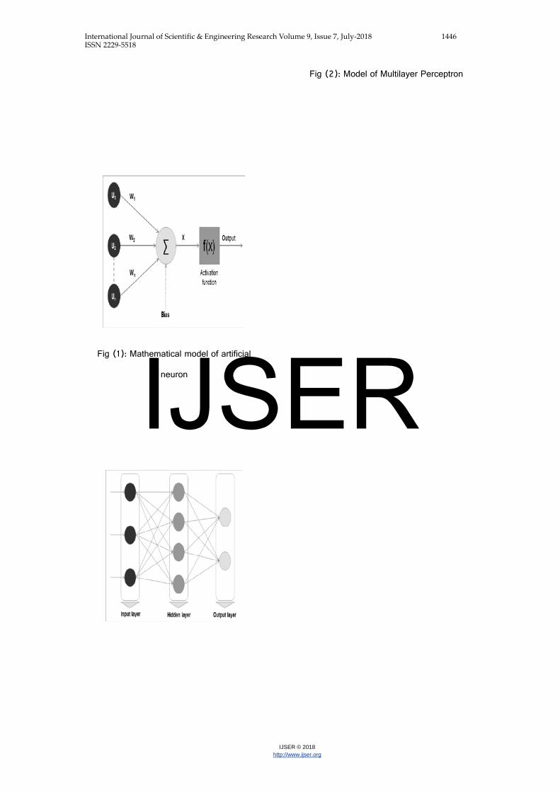
the Artificial Neural Network (ANN) shown in
Fig(1) has powerful mathematical models
and universal predictors that have been used
to solve various real-world problems. Among
different types of ANNs, multilayered
perceptron (MLP) with well-known structure
as in Fig(2) represent the best, and consists
of three layers; the input layer, hidden layer
and output layer, with every layer consisting
of several neurons. The neurons are
connected to each other's by a set of
synaptic weights, which consists of values
representing the strength of the connection.
After applying the suitable dataset and during
the training phase , the ANN continuously
adjusts the values of these weights until it
reaches a certain termination condition,
usually measured by the performance of
mean squared error value of the network ,
maximum allowable training time duration,
the number of maximum iterations or epochs
[11].
IJSER

International Journal of Scientific & Engineering Research Volume 9, Issue 7, July-2018 1439 ISSN 2229-5518
IJSER © 2018 http://www.ijser.org
Among of various learning algorithms have
been used for training of ANNs, the most
well-known technique used to train the ANN
is still the backpropagation (BP) algorithm
The BP algorithm has a dramatic acceptance
by the researchers due to its robustness and
versatility while giving the most efficient
learning algorithm for MLP networks. In
addition, it is a gradient-descent based
algorithm which upgraded the weights of
ANN by using the gradients of their error in
each iteration. so, the adjustments on every
weight achieved by considering how much
they affect the final output, and this offers a
more refined local minimum searching
capability while the process still keep looking
for the global minimum. The BP algorithm
using the same dataset by iterates and
iterates again till the network converges to
the searched minimum point. Generally, as
the number of trained epochs and data-set
samples increases, the accuracy and
precision of the ANN to expect the output
increases, but this will cause a longer
training time, so there is a tradeoff between
the time and accuracy in the training phase
of the ANN [12].
From a technology point of view, last years
WSN have attracted the interest of most
researchers whereas many industrial
branches with different applications are used
WSN in different industrial fields. There are
variety of methods in order to adopt abrupt
development changes in technology for
communication and wireless instrumentation
industry on the basis of Electronics and
Computers. Regarding remote control based
on Zigbee and Wi-Fi protocols due to
limitation of wide band frequency and low
speed in data transmission that is
appropriate for small plant and cannot be
used for massive plants for oil pipelines.
Therefore these problems have tendency to
lead us towards WSN which is based on
zigbee protocol. Structures of WSN are three
layers. End device Sensor node, consists of
voltage and current transducers which are
placed in the first layer. Microcontroller which
IJSER

International Journal of Scientific & Engineering Research Volume 9, Issue 7, July-2018 1440 ISSN 2229-5518
IJSER © 2018 http://www.ijser.org
is needed for the processing and wireless
communication along with the servers also
locates in this layer. The Second one is
router which is the responsible for
retransmission the data from the end device
to the coordinator . The third is the core for
the WSN including the intelligent algorithms
installed in an intelligent controller to lead the
whole data coming from sensor and give a
final decision for the actuators or make any
advanced or speed processing [13].
It seems there is a global agreement that a
major problem for most ANN researchers are
facing is in selecting the suitable ANN
topology. However according to literatures ,
the influence of the network topology on the
final output is tremendous despite not having
a direct interaction with the external
environment. And hence the influence of this
network topology on the output will be
consequently reflected in the form of other
new problems, such as the slow
convergence rate, and getting trapped in
local minima. In this instant , there have
been no officially established methods to
determine the optimal topology of an ANN for
any given problem, and this will e extended
to the other layers especially in the number
of neurons for the hidden layer. If the
number of neurons is inadequate, it may
result in under-fitting, which means that the
neural network will be unable to learn all the
information contained in the applied dataset.
Conversely, an overabundance of neurons in
the hidden layer will lead to over-fitting, a
situation in which the neural network hold
the noise of the training data-set, negatively
impacting its ability to predict new data in
future[14].
Some literature and papers may offer rules
of thumb methods or guidelines for selecting
the number of adequate hidden neurons by
using any value between the number of input
and output neurons for the ANN, but a good
topology cannot be decided solely based on
the number of inputs and outputs neurons
alone [15].
IJSER
International Journal of Scientific & Engineering Research Volume 9, Issue 7, July-2018 1441 ISSN 2229-5518
IJSER © 2018 http://www.ijser.org
2- Theoretical background
The multilayer feedforward neural network is
the core of the artificial Neural Network. It
can be used for both data fitting and pattern
recognition assignments. With the addition of
a new proposed tapped delay line, it can also
be used for system model prediction. The
training functions described in this paper are
not limited to multilayer networks. They can
be used to train arbitrary network
architectures (even hybrid networks), as long
as their components are differentiable [16].
The procedure for the artificial neural network
design summarized by about seven primary
steps described hereunder:
a) Collect input / output data-set
b) Create the network structure
c) Configure the network topology
d) Initialize the weights and biases for all
neurons
e) Train the neural network
f) Validate the network results (post-
training analysis).
g) Use the network for the new real
input.
Noting that first Step should be happened
outside the framework of artificial Neural
Network programming, but this step is critical
to the success of the whole design process,
such that the ANN will simulate the real
system response for the new test input, as it
was already trained by an actual data-set
[17].
When the network weights and biases are
initialized, the network is ready for training.
The multilayer feed forward neural network
can be trained for function fitting (as a
nonlinear regression) or pattern recognition
problem. The training process requires a set
of samples from a proper network behavior, it
means network input vector P and target
output vector T [18].
The training process of a neural network try
to tune the values of the weights and biases
of the network neurons in each of hidden and
output layers, to optimize network
IJSER

International Journal of Scientific & Engineering Research Volume 9, Issue 7, July-2018 1442 ISSN 2229-5518
IJSER © 2018 http://www.ijser.org
performance, as defined by the network
performance function which is (for most MLP
neural network) mean square error MSE,
that represent the average squared error
between the network outputs Y and the
target outputs T [19].
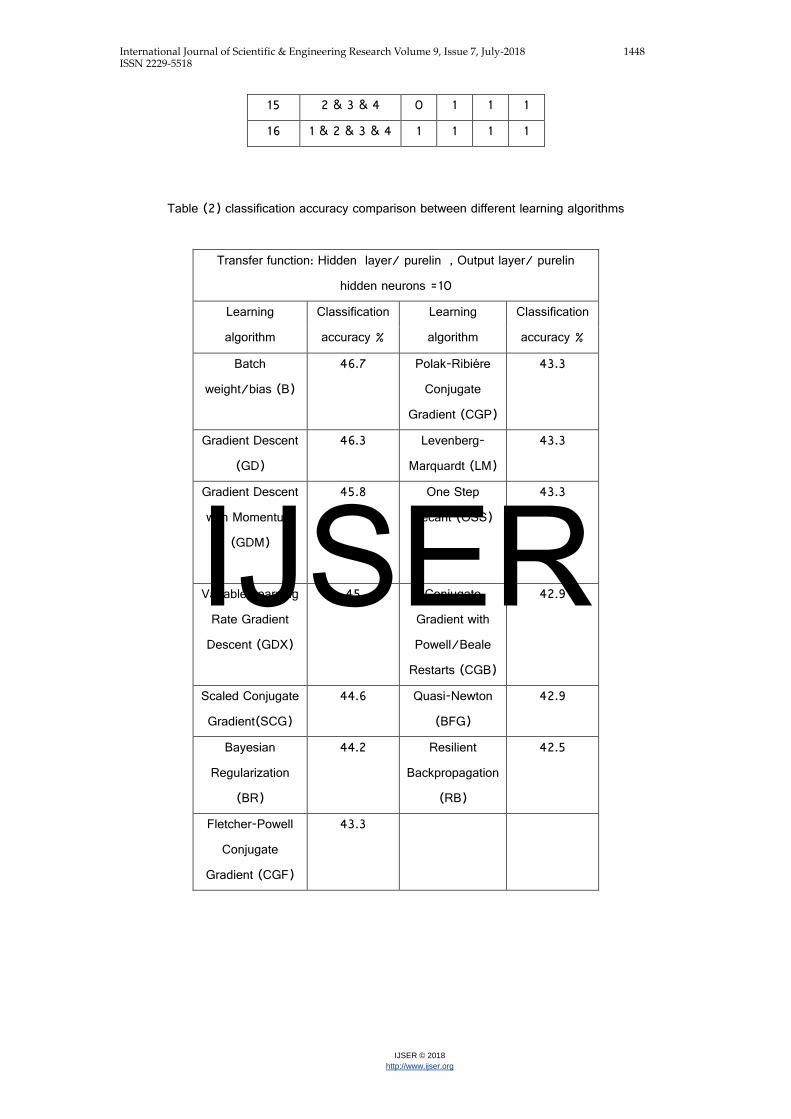
Training of BPNN can be achieved via two
methods; either incremental method or batch
method. In incremental method, the gradient
of error is computed and the weights are
updated after each applied input. Unlikely, In
batch method, the weights are updated after
all the inputs in the training set are applied to
the network. Based on results in table (2)
Batch training algorithm is noticeably fast
and produces smaller errors than other
incremental training algorithms[20].
Any standard numerical optimization
algorithm can be used For training multilayer
feedforward networks, however, to optimize
the performance function, there are a some
optimization methods that have shown
excellent minimization error performance for
neural network training. These optimization
methods use either the performance gradient
of the network with referred to the weights, or
the Jacobian of the network errors with
respect to the weights. The gradient and the
Jacobian are calculated using a procedure
known as backpropagation algorithm, within
which computations are performed backward
through the network [21].
The term “backpropagation” in some
literatures, ambiguously used to point to the
gradient descent algorithm specifically, when
applied to neural network principles. But in
this work terminology is used precisely,
since the process of the gradient and
Jacobian calculations backward through the
network is applied in all the used training
functions in this work. It is clearer to use the
name of the specific optimization algorithm
that is being used, rather than to use the
term backpropagation alone [22].
Another millstone terminology is, sometimes
the multilayer network is referred to as a
backpropagation network. But, the
backpropagation way that is used to
IJSER

International Journal of Scientific & Engineering Research Volume 9, Issue 7, July-2018 1443 ISSN 2229-5518
IJSER © 2018 http://www.ijser.org
calculate Jacobians and gradients in a
multilayer network can also be used for many
different neural network architectures [23].
3- Block diagram proposed model
The block diagram for the proposed
experimental system is shown in Figure
(3).The details of different operating
parameters and material parts of the
system are given in table (4).
Each leak size is given a certain output class
which in turn after combination with other
classes compromise a classification code for
the output layer as per table (1) to control
the classification problem with BP ANN.
Experimental set up is consists of a pipeline
having length of 7m & diameter of 2 inch
,The pipeline has four sections 1, 2, 3 & 4
having length of 1.5m each.
Pipeline sections are connected using a
flange assembly. while every flange has an
orifice plate & rubber gasket that are placed
between them. Also 4 nut-bolts each has
diameter 0.5 inch are used for each section
of the assembly. Two tapings are provided
for manometer connection at suitable
positions across the flanges.
In order to measure the pressure drop four
inverted manometers are connected in each
section, a sump with capacity 500 liters is
used. While oil is flowing into the pipeline
using 1 hp motor oil pump.
Dropped oil is returned to the sump using
other 3 inch pipeline, pressure drop across
the orifice in each section can be recorded
by varying the oil flow-rates at normal
conditions. Leak positions are artificially
generated by creating a hole in the pipeline
at different positions from the flanges as
explained in table (4).
4- Experimental results and discussion
Referring to the simulation results at Fig(4)
to Fig(17), the fastest training function is
IJSER
International Journal of Scientific & Engineering Research Volume 9, Issue 7, July-2018 1444 ISSN 2229-5518
IJSER © 2018 http://www.ijser.org
generally Levenberg-Marquardt .However,
The quasi-Newton method, is also quite fast.
Although both of these methods tend to be
inefficient for large networks (with thousands
of neurons weights), because they need
more memory and more computation time for
these weights upgraded. In fact, Levenberg-
Marquardt algorithm performs better on curve
fitting (as a nonlinear regression)
assignments than on pattern recognition
assignments see Fig (10) through Fig (17).
On the other hand, when large networks are
training, or pattern recognition problems to
be solved, Resilient Backpropagation and
Scaled Conjugate Gradient are better choices
due to their minimum memory requirements,
and yet they are much faster than other
classical gradient descent algorithms.
Referring to Fig (4) through Fig (9),
sometimes the network is not sufficiently
accurate, and in order to improve the
performance some points are followed:
a) The process is re-initialized and the
network is trained again. In order to
get new solutions.
b) The number of hidden neurons are
increased .keeping that, larger
numbers of hidden layer neurons of
course give the network more
flexibility because the network will
have more candidate optimization
parameters.
c) A different training algorithms, such as
Bayesian regularization training can
sometimes produce better
generalization capability than using
early stopping.
d) Finally, by using additional training
data-set (if possible). Off course
additional data delivery for the
network is more likely to produce a
network that will perform excellence
to new data.
IJSER

International Journal of Scientific & Engineering Research Volume 9, Issue 7, July-2018 1445 ISSN 2229-5518
IJSER © 2018 http://www.ijser.org
5- Conclusions and recommendations
The main objective of the present paper was
to emphases the possibility of using an
ANN in leak detection system in oil pipelines.
For this reason, experimental data was
generated for normal and leaked conditions
for flow of oil in a pipeline. Tiny holes were
created artificially for generating leak
conditions at different locations on the
pipeline. Pressure drop across the orifice are
placed at four positions in the pipeline to be
used for recording these normal & leak
conditions. ANN models with different
scenario were developed that detect the
existing of leak or not as a binary
classification problem. Also, pressure drop
was simulated at four different locations with
different leak size ranged from 0.25'' up to
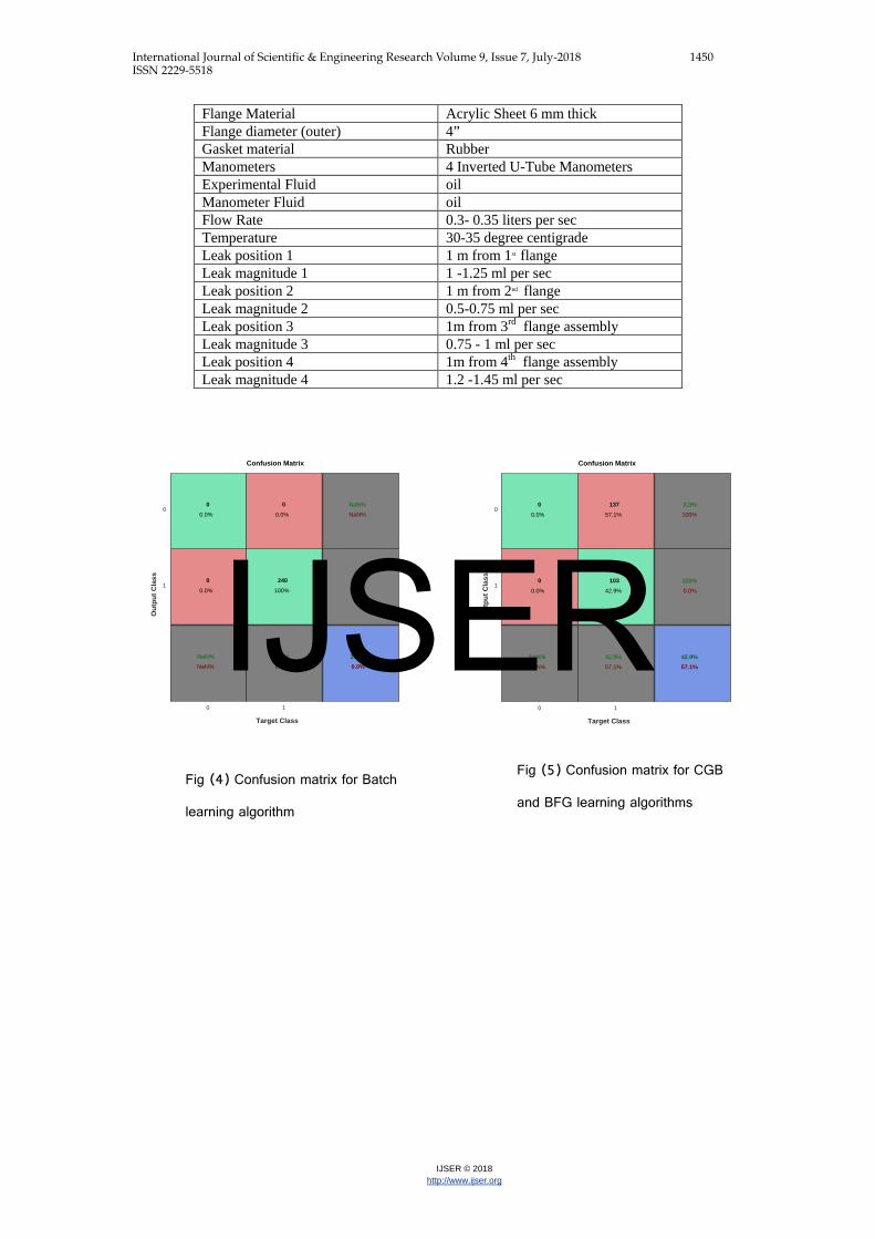
1'' in step of 0.25. The accuracy of prediction
of these classification models is calculated
and seen to be 100% via confusion matrix
form and validated for 240 samples of the
pressure data set for training the ANN
divided as 168 samples for training and 36
samples for each of validation and testing
phases of the training process. Based on the
results and discussions, it can be said that all
the ANN models developed in the present
work are accurate in classification for leak
existing and its size estimation . It can be
thus generally concluded that, ANN can be
efficiently deployed in developing a
mathematical model that can be used as a
classifier for the data which may be available
for industrial field at normal or faulty
conditions from oil and gas pipeline.
IJSER
International Journal of Scientific & Engineering Research Volume 9, Issue 7, July-2018 1446 ISSN 2229-5518
IJSER © 2018 http://www.ijser.org
Fig (1): Mathematical model of artificial
neuron
Fig (2): Model of Multilayer Perceptron
IJSER

International Journal of Scientific & Engineering Research Volume 9, Issue 7, July-2018 1447 ISSN 2229-5518
IJSER © 2018 http://www.ijser.org
Fig(3) block diagram for the proposed experimental leak detection system
Table (1) States for classifying the simulated proposed system
State Leak position F1 F2 F3 F4
1 No leak 0 0 0 0
2 1 1 0 0 0
3 2 0 1 0 0
4 3 0 0 1 0
5 4 0 0 0 1
6 1 & 2 1 1 0 0
7 1 & 3 1 0 1 0
8 1 & 4 1 0 0 1
9 2 & 3 0 1 1 0
10 2 & 4 0 1 0 1
11 3 & 4 0 0 1 1
12 1 & 2 & 3 1 1 1 0
13 1 & 2 & 4 1 1 0 1
14 1 & 3 & 4 1 0 1 1
IJSER
International Journal of Scientific & Engineering Research Volume 9, Issue 7, July-2018 1448 ISSN 2229-5518
IJSER © 2018 http://www.ijser.org
15 2 & 3 & 4 0 1 1 1
16 1 & 2 & 3 & 4 1 1 1 1
Table (2) classification accuracy comparison between different learning algorithms
Transfer function: Hidden layer/ purelin , Output layer/ purelin
hidden neurons =10
Learning
algorithm
Classification
accuracy %
Learning
algorithm
Classification
accuracy %
Batch
weight/bias (B)
46.7 Polak-Ribiére
Conjugate
Gradient (CGP)
43.3
Gradient Descent
(GD)
46.3 Levenberg-
Marquardt (LM)
43.3
Gradient Descent
with Momentum
(GDM)
45.8 One Step
Secant (OSS)
43.3
Variable Learning
Rate Gradient
Descent (GDX)
45 Conjugate
Gradient with
Powell/Beale
Restarts (CGB)
42.9
Scaled Conjugate
Gradient(SCG)
44.6 Quasi-Newton
(BFG)
42.9
Bayesian
Regularization
(BR)
44.2 Resilient
Backpropagation
(RB)
42.5
Fletcher-Powell
Conjugate
Gradient (CGF)
43.3
IJSER
International Journal of Scientific & Engineering Research Volume 9, Issue 7, July-2018 1449 ISSN 2229-5518
IJSER © 2018 http://www.ijser.org
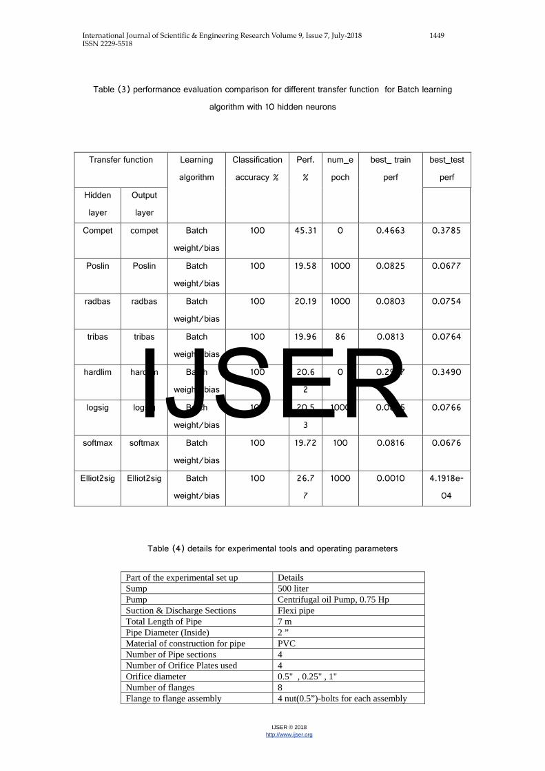
Table (3) performance evaluation comparison for different transfer function for Batch learning
algorithm with 10 hidden neurons
Transfer function Learning
algorithm
Classification
accuracy %
Perf.
%
num_e
poch
best_ train
perf
best_test
perf
Hidden
layer
Output
layer
Compet compet Batch
weight/bias
100 45.31 0 0.4663 0.3785
Poslin Poslin Batch
weight/bias
100 19.58 1000 0.0825
0.0677
radbas radbas Batch
weight/bias
100 20.19 1000 0.0803 0.0754
tribas tribas Batch
weight/bias
100 19.96 86 0.0813 0.0764
hardlim hardlim Batch
weight/bias
100 20.6
2
0 0.2987 0.3490
logsig logsig Batch
weight/bias
100 20.5
3
1000 0.0805 0.0766
softmax softmax Batch
weight/bias
100 19.72 100 0.0816 0.0676
Elliot2sig Elliot2sig Batch
weight/bias
100 26.7
7
1000 0.0010 4.1918e-
04
Table (4) details for experimental tools and operating parameters
Part of the experimental set up Details Sump 500 liter Pump Centrifugal oil Pump, 0.75 Hp Suction & Discharge Sections Flexi pipe Total Length of Pipe 7 m Pipe Diameter (Inside) 2 ” Material of construction for pipe PVC Number of Pipe sections 4 Number of Orifice Plates used 4 Orifice diameter 0.5" , 0.25" , 1" Number of flanges 8 Flange to flange assembly 4 nut(0.5”)-bolts for each assembly
IJSER
International Journal of Scientific & Engineering Research Volume 9, Issue 7, July-2018 1450 ISSN 2229-5518
IJSER © 2018 http://www.ijser.org
Flange Material Acrylic Sheet 6 mm thick Flange diameter (outer) 4” Gasket material Rubber Manometers 4 Inverted U-Tube Manometers Experimental Fluid oil Manometer Fluid oil Flow Rate 0.3- 0.35 liters per sec Temperature 30-35 degree centigrade Leak position 1 1 m from 1st flange Leak magnitude 1 1 -1.25 ml per sec Leak position 2 1 m from 2nd flange Leak magnitude 2 0.5-0.75 ml per sec Leak position 3 1m from 3rd flange assembly Leak magnitude 3 0.75 - 1 ml per sec Leak position 4 1m from 4th flange assembly Leak magnitude 4 1.2 -1.45 ml per sec
Fig (4) Confusion matrix for Batch
learning algorithm
Fig (5) Confusion matrix for CGB
and BFG learning algorithms
0 1
Target Class
0
1
Out
put C
lass
Confusion Matrix
00.0%
00.0%
NaN%NaN%
00.0%
240100%
100%0.0%
NaN%NaN%
100%0.0%
100%0.0%
0 1
Target Class
0
1
Out
put C
lass
Confusion Matrix
00.0%
00.0%
NaN%NaN%
13757.1%
10342.9%
42.9%57.1%
0.0%100%
100%0.0%
42.9%57.1%IJSER
International Journal of Scientific & Engineering Research Volume 9, Issue 7, July-2018 1451 ISSN 2229-5518
IJSER © 2018 http://www.ijser.org
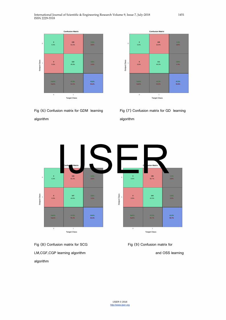
Fig (6) Confusion matrix for GDM learning
algorithm
Fig (7) Confusion matrix for GD learning
algorithm
Fig (8) Confusion matrix for SCG Fig (9) Confusion matrix for
LM,CGF,CGP learning algorithm and OSS learning
algorithm
0 1
Target Class
0
1
Out
put C
lass
Confusion Matrix
00.0%
00.0%
NaN%NaN%
13054.2%
11045.8%
45.8%54.2%
0.0%100%
100%0.0%
45.8%54.2%
0 1
Target Class
0
1
Out
put C
lass
Confusion Matrix
00.0%
00.0%
NaN%NaN%
12953.8%
11146.3%
46.3%53.8%
0.0%100%
100%0.0%
46.3%53.8%
0 1
Target Class
0
1
Out
put C
lass
Confusion Matrix
00.0%
00.0%
NaN%NaN%
13656.7%
10443.3%
43.3%56.7%
0.0%100%
100%0.0%
43.3%56.7%
0 1
Target Class
0
1
Out
put C
lass
Confusion Matrix
00.0%
00.0%
NaN%NaN%
13355.4%
10744.6%
44.6%55.4%
0.0%100%
100%0.0%
44.6%55.4%
IJSER

International Journal of Scientific & Engineering Research Volume 9, Issue 7, July-2018 1452 ISSN 2229-5518
IJSER © 2018 http://www.ijser.org
Fig(10) Training with Elliot2sig transfer Fig(11) Training with Softmax transfer
function for hidden and output layers function for hidden and output layers
IJSER

International Journal of Scientific & Engineering Research Volume 9, Issue 7, July-2018 1453 ISSN 2229-5518
IJSER © 2018 http://www.ijser.org
Fig (12) Training with Logsig transfer Fig (13)Training with Hardlim
transfer
function for hidden and output layers function for hidden and output
layers
Fig (14) Training with Tribas transfer Fig (15) Training with Radbas transfer
function for hidden and output layers function for hidden and output layers
IJSER
International Journal of Scientific & Engineering Research Volume 9, Issue 7, July-2018 1454 ISSN 2229-5518
IJSER © 2018 http://www.ijser.org
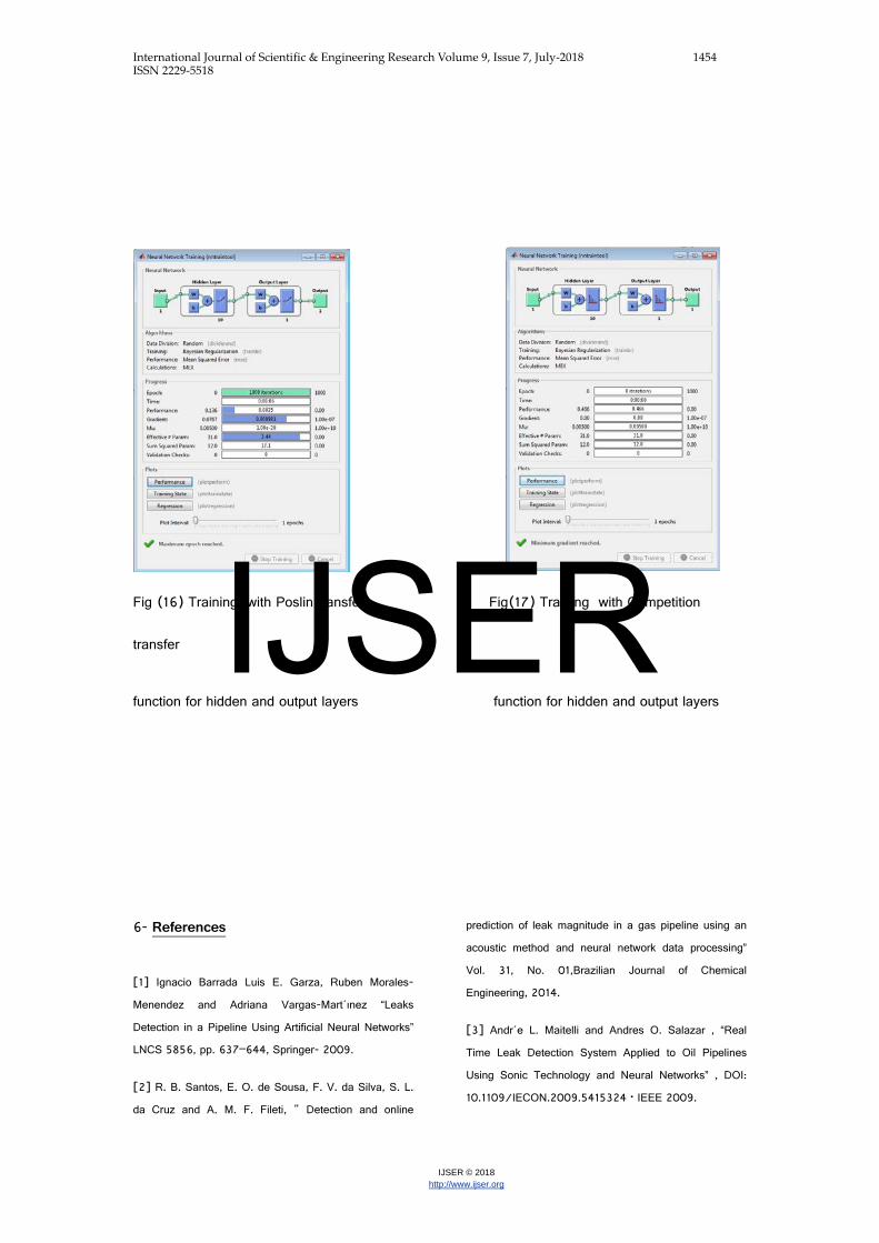
Fig (16) Training with Poslin transfer Fig(17) Training with Competition
transfer
function for hidden and output layers function for hidden and output layers
6- References
[1] Ignacio Barrada Luis E. Garza, Ruben Morales-
Menendez and Adriana Vargas-Mart´ınez “Leaks
Detection in a Pipeline Using Artificial Neural Networks”
LNCS 5856, pp. 637–644, Springer- 2009.
[2] R. B. Santos, E. O. de Sousa, F. V. da Silva, S. L.
da Cruz and A. M. F. Fileti, " Detection and online
prediction of leak magnitude in a gas pipeline using an
acoustic method and neural network data processing”
Vol. 31, No. 01,Brazilian Journal of Chemical
Engineering, 2014.
[3] Andr´e L. Maitelli and Andres O. Salazar , “Real
Time Leak Detection System Applied to Oil Pipelines
Using Sonic Technology and Neural Networks” , DOI:
10.1109/IECON.2009.5415324 · IEEE 2009.
IJSER

International Journal of Scientific & Engineering Research Volume 9, Issue 7, July-2018 1455 ISSN 2229-5518
IJSER © 2018 http://www.ijser.org
[4] P. Rajeev, J. Kodikara, W. K. Chiu and T. Kuen,
“Distributed Optical Sensors And Their Applications In
Pipeline Monitoring,” Key Engineering Materials Vol. 558
, pp 424-434, 2013.
[5] Morteza Mohammadzaheri, “Fault Detection of Gas
Pipelines Using Mechanical Waves and Intelligent
Techniques "Conference Paper 2015.
[6] L. Molina-Espinosa , C.G. Aguilar-Madera , E.C.
Herrera-Hernández, C. Verde “Numerical modeling of
pseudo-homogeneous fluid flow in a pipe with leaks”
Computers and Mathematics, Elsevier Ltd. 2017.
[7] Budi Santoso · Indarto · Deendarlianto , “Pipeline
Leak Detection in Two Phase Flow Based on Fluctuation
Pressure Difference and Artificial Neural Network (ANN)
“Jan 2014.
[8] L. Kong, M. Xia, X. Y. Liu, G. Chen, Y. Gu, M. Y.
Wu, and X. Liu, “Data loss and reconstruction in wireless
sensor networks,” Proceedings-IEEE INFOCOM vol. 25,
no. 11, pp. 2818-2828, 2014.
[9] N F Adnan, M F Ghazali, M M Amin and A M A
Hamat, “Leak detection in gas pipeline by acoustic and
signal processing – A review” IOP Conf. Series:
Materials Science and Engineering (ICMER) 2015.
[10] Xiaoliang Zhu, Li Du1, Bendong Liu and Jiang Zhe,
“A microsensor array for quantification of lubricant
contaminants using a back propagation artificial neural
network” Article in Journal of Micromechanics and
Microengineering • June 2016.
[11] F. Tao, Y. Zuo, L. Da Xu, & L. Zhang, “IoT-based
intelligent perception and access of manufacturing
resource toward cloud manufacturing,” IEEE
Transactions on Industrial Informatics, vol. 10 No2, pp.
1547-1557, 2014.
[12] Zhang, J., Zhang, J., Lok, T. and Lyu, M., "A
hybrid particle swarm optimization-back-propagation
algorithm
[13] M.S. Pan, P. L. Liu, and Y.P. Lin, “Event data
collection in ZigBee treebased wireless sensor
networks,” Computer Networks, vol. 73, 2014.
[14] Hagan, M.T., and M. Menhaj, “Training feed-
forward networks with the Marquardt algorithm,” IEEE
Transactions on Neural Networks, Vol. 5, No. 6, 1999,
pp.
989–993, 1994.
[15] Moller, M.F., “A scaled conjugate gradient
algorithm for fast supervised learning,” Neural Networks,
Vol. 6, 1993, pp. 525–533.
[16] Y. X. Liu and X. X. Yuan, “Applications of fuzzy
reasoning techniques and neural network in fire
detection system”, Computer Measurement & Control,
vol. 21, no. 12, (2013).
[17] L. Hamm, B. W. Brorsen and M. T. Hagan,
“Comparison of Stochastic Global Optimization Methods
to Estimate Neural Network Weights,” Neural Processing
Letters, vol. 26, no. 3, December 2007. (Chapter 22).
[18] P.M. Agrawal, A.N.A. Samadh, L.M. Raff, M.
Hagan, S. T. Bukkapatnam, and R. Komanduri,
“Prediction of molecular- dynamics simulation results
using feedforward neural networks: Reaction of a C2
dimer with an activated diamond (100) surface,” The
Journal of Chemical Physics 123, 224711, 2005.
(Chapter 24).
[19] M. Phan and M. Hagan, “Error Surface of
Recurrent Networks,” IEEE Transactions on Neural
Networks and Learning Systems, vol. 24, no. 11, pp.
1709 - 1721, October, 2013. (Chapter 14).
[20] X. J. Zhang, “Fire alarm system based on BP
neural network and D-S Evidence Theory”, Instrument
Technique and Sensor, vol. 1, (2011).
[21] De Jesús, O., and M.T. Hagan, “Backpropagation
Algorithms for a Broad Class of Dynamic Networks,”
IJSER

International Journal of Scientific & Engineering Research Volume 9, Issue 7, July-2018 1456 ISSN 2229-5518
IJSER © 2018 http://www.ijser.org
IEEE Transactions on Neural Networks, Vol. 18, No. 1,
pp. 14 -27, January 2007.
[22] C. Ren, W. Qiao and X. Tian, "Natural gas
pipeline corrosion rate prediction model based on bp
neural network," in Fuzzy Engineering and Operations
Research, Berlin, Springer, pp. 449-455, 2012.
[23] Khan, K. and Sahai, A., "A comparison of BA, GA,
PSO, BP and LM for training feedforward neural
networks in e-learning context," Intelligent Systems and
Applications, vol. 7, pp. 23-29, 2012.
IJSER