University of Pennsylvania University of Pennsylvania

ScholarlyCommons ScholarlyCommons

Real-Time and Embedded Systems Lab (mLAB) School of Engineering and Applied Science

2016

DR-Advisor: A Data-Driven Demand Response Recommender DR-Advisor: A Data-Driven Demand Response Recommender

System System

Madhur Behl University of Pennsylvania, mbehl@seas.upenn.edu

Francesco Smarra Universita` degli Studi dell’Aquila, francesco.smarra@univaq.it

Rahul Mangharam University of Pennsylvania, rahulm@seas.upenn.edu

Follow this and additional works at: https://repository.upenn.edu/mlab_papers

Part of the Computer Engineering Commons, and the Electrical and Computer Engineering Commons

Recommended Citation Recommended Citation Madhur Behl, Francesco Smarra, and Rahul Mangharam, "DR-Advisor: A Data-Driven Demand Response Recommender System", Journal of Applied Energy . January 2016.

This paper is posted at ScholarlyCommons. https://repository.upenn.edu/mlab_papers/83 For more information, please contact repository@pobox.upenn.edu.

DR-Advisor: A Data-Driven Demand Response Recommender System DR-Advisor: A Data-Driven Demand Response Recommender System

Abstract Abstract Demand response (DR) is becoming increasingly important as the volatility on the grid continues to increase. Current DR ap- proaches are predominantly completely manual and rule-based or involve deriving first principles based models which are ex- tremely cost and time prohibitive to build. We consider the problem of data-driven end-user DR for large buildings which involves predicting the demand response baseline, evaluating fixed rule based DR strategies and synthesizing DR control actions. The challenge is in evaluating and taking control decisions at fast time scales in order to curtail the power consumption of the building, in return for a financial reward. We provide a model based control with regression trees algorithm (mbCRT), which allows us to perform closed-loop control for DR strategy synthesis for large commercial buildings. Our data-driven control synthesis algorithm outperforms rule-based DR by 17% for a large DoE commercial reference building and leads to a curtailment of 380kW and over $45, 000 in savings. Our methods have been integrated into an open source tool called DR-Advisor, which acts as a recommender system for the building’s facilities manager and provides suitable control actions to meet the desired load curtailment while main- taining operations and maximizing the economic reward. DR-Advisor achieves 92.8% to 98.9% prediction accuracy for 8 buildings on Penn’s campus. We compare DR-Advisor with other data driven methods and rank 2nd on ASHRAE’s benchmarking data-set for energy prediction.

Keywords Keywords CPS, data-driven, machine learning, demand response, energy, buildings

Disciplines Disciplines Computer Engineering | Electrical and Computer Engineering

This journal article is available at ScholarlyCommons: https://repository.upenn.edu/mlab_papers/83

Applied Energy 00 (2016) 1–25

AppliedEnergy

DR-Advisor: A Data-Driven Demand Response RecommenderSystem

Madhur Behla, Francesco Smarrab, Rahul Mangharama

aDept. of Electrical and Systems Engineering,University of Pennsylvania,

Philadelphia, USAbDepartment of Information Engineering, Computer Science and Mathematics,

Universita degli Studi dell’Aquila,L’Aquila, Italy

AbstractDemand response (DR) is becoming increasingly important as the volatility on the grid continues to increase. Current DR ap-proaches are predominantly completely manual and rule-based or involve deriving first principles based models which are ex-tremely cost and time prohibitive to build. We consider the problem of data-driven end-user DR for large buildings which involvespredicting the demand response baseline, evaluating fixed rule based DR strategies and synthesizing DR control actions. Thechallenge is in evaluating and taking control decisions at fast time scales in order to curtail the power consumption of the building,in return for a financial reward. We provide a model based control with regression trees algorithm (mbCRT), which allows us toperform closed-loop control for DR strategy synthesis for large commercial buildings. Our data-driven control synthesis algorithmoutperforms rule-based DR by 17% for a large DoE commercial reference building and leads to a curtailment of 380kW and over$45, 000 in savings. Our methods have been integrated into an open source tool called DR-Advisor, which acts as a recommendersystem for the building’s facilities manager and provides suitable control actions to meet the desired load curtailment while main-taining operations and maximizing the economic reward. DR-Advisor achieves 92.8% to 98.9% prediction accuracy for 8 buildingson Penn’s campus. We compare DR-Advisor with other data driven methods and rank 2nd on ASHRAE’s benchmarking data-setfor energy prediction.

c© 2015 Submitted to Applied Energy

Keywords:Demand Response, Regression trees, data-driven control, machine learning, Electricity curtailment, Demand side management

1. Introduction1

In 2013, a report by the U.S. National Climate Assessment provided evidence that the most recent decade was the2

nation’s warmest on record [1] and experts predict that temperatures are only going to rise. In fact, the year 2015 is3

very likely to become the hottest year on record since the beginning of weather recording in 1880 [2]. Heat waves in4

summer and polar vortexes in winter are growing longer and pose increasing challenges to an already over-stressed5

electric grid.6

Email addresses: mbehl@seas.upenn.edu (Madhur Behl), francesco.smarra@univaq.it (Francesco Smarra),rahulm@seas.upenn.edu (Rahul Mangharam)

1

Behl et al. / Applied Energy 00 (2016) 1–25 2

Furthermore, with the increasing penetration of renewable generation, the electricity grid is also experiencing7

a shift from predictable and dispatchable electricity generation to variable and non-dispatchable generation. This8

adds another level of uncertainty and volatility to the electricity grid as the relative proportion of variable generation9

vs. traditional dispatchable generation increases. The organized electricity markets across the world all use some10

variant of real-time price for wholesale electricity. The real-time electricity market at PJM, one of the world’s largest11

independent system operator (ISO), is a spot market where electricity prices are calculated at five-minute intervals12

based on the grid operating conditions. The volatility due to the mismatch between electricity generation and supply13

further leads to volatility in the wholesale price of electricity. For e.g., the polar vortex triggered extreme weather14

events in the U.S. in January 2014, which caused many electricity customers to experience increased costs. Parts of15

the PJM electricity grid experienced a 86 fold increase in the price of electricity from $31/MW h to $2, 680/MW hin a16

matter of a few minutes [3]. Similarly, the summer price spiked 32 fold from an average of $25/MW h to $800/MW h17

in July of 2015. Such events show how unforeseen and uncontrollable circumstances can greatly affect electricity18

prices that impact ISOs, suppliers, and customers. Energy industry experts are now considering the concept that19

extreme weather, more renewables and resulting electricity price volatility, could become the new norm.20

Across the United States, electric utilities and ISOs are devoting increasing attention and resources to demand21

response (DR) [4]. Demand response is considered as a reliable means of mitigating the uncertainty and volatility22

of renewable generation and extreme weather conditions and improving the grid’s efficiency and reliability. The23

potential demand response resource contribution from all U.S. demand response programs is estimated to be nearly24

72,000 megawatts (MW), or about 9.2 percent of U.S. peak demand [5] making DR the largest virtual generator in25

the U.S. national grid. The annual revenue to end-users from DR markets with PJM ISO alone is more than $70026

million [6]. Global DR revenue is expected to reach nearly $40 billion from 2014 through 2023 [7].27

The volatility in real-time electricity prices poses the biggest operational and financial risk for large scale end-users28

of electricity such as large commercial buildings, industries and institutions [8]; often referred to as C/I/I consumers.29

In order to shield themselves from the volatility and risk of high prices, such consumers must be more flexible in30

their electricity demand. Consequently, large C/I/I customers are increasingly looking to demand response programs31

to help manage their electricity costs.32

DR programs involve a voluntary response of a building to a price signal or a load curtailment request from the33

utility or the curtailment service provider (CSP). Upon successfully meeting the required curtailment level the end-34

users are financially rewarded, but may also incur penalties for under-performing and not meeting a required level35

of load curtailment. On the surface demand response may seem simple. Reduce your power when asked to and get36

paid. However, in practice, one of the biggest challenges with end-user demand response for large scale consumers37

of electricity is the following: Upon receiving the notification for a DR event, what actions must the end-user take38

in order to achieve an adequate and a sustained DR curtailment? This is a hard question to answer because of the39

following reasons:40

1. Modeling complexity and heterogeneity: Unlike the automobile or the aircraft industry, each building is de-41

signed and used in a different way and therefore, it must be uniquely modeled. Learning predictive models of42

building’s dynamics using first principles based approaches (e.g., with EnergyPlus [9]) is very cost and time43

prohibitive and requires retrofitting the building with several sensors [10]; The user expertise, time, and associ-44

ated sensor costs required to develop a model of a single building is very high. This is because usually a building45

modeling domain expert typically uses a software tool to create the geometry of a building from the building46

design and equipment layout plans, add detailed information about material properties, about equipment and47

operational schedules. There is always a gap between the modeled and the real building and the domain expert48

must then manually tune the model to match the measured data from the building [11].49

2. Limitations of rule-based DR: The building’s operating conditions, internal thermal disturbances and envi-50

ronmental conditions must all be taken into account to make appropriate DR control decisions, which is not51

possible with using rule-based and pre-determined DR strategies since they do not account for the state of the52

building but are instead based on best practices and rules of thumb. As shown in Fig. 1(a), the performance53

of a rule-based DR strategy is inconsistent and can lead to reduced amount of curtailment which could result54

in penalties to the end-user. In our work, we show how a data-driven DR algorithm outperforms a rule-based55

strategy by 17% while accounting for thermal comfort. Rule based DR strategies have the advantage of being56

2

Behl et al. / Applied Energy 00 (2016) 1–25 3

Figure 1: Majority of DR today is manual and rule-based. (a) The fixed rule based DR is inconsistent and could under-perform compared to therequired curtailment, resulting in DR penalties. (b) Using data-driven models DR-Advisor uses DR strategy evaluation and DR strategy synthesisfor a sustained and sufficient curtailment.

simple but they do not account for the state of the building and weather conditions during a DR event. Despite57

this lack of predictability, rule-based DR strategies account for the majority of DR approaches.58

3. Control complexity and scalability: Upon receiving a notification for a DR event, the building’s facilities59

manager must determine an appropriate DR strategy to achieve the required load curtailment. These control60

strategies can include adjusting zone temperature set-points, supply air temperature and chilled water tempera-61

ture set-point, dimming or turning off lights, decreasing duct static pressure set-points and restricting the supply62

fan operation etc.. In a large building, it is difficult to asses the effect of one control action on other sub-systems63

and on the building’s overall power consumption because the building sub-systems are tightly coupled. Con-64

sider the case of the University of Pennsylvania’s campus, which has over a hundred different buildings and65

centralized chiller plants. In order to perform campus wide DR, the facilities manager must account for several66

hundred thousand set-points and their impact on the different buildings. Therefore, it is extremely difficult for a67

human operator to accurately gauge the building’s or a campus’s response.68

4. Interpretability of modeling and control: Predictive models for buildings, regardless how sophisticated, lose69

their effectiveness unless they can be interpreted by human experts and facilities managers in the field. For70

e.g., artificial neural networks (ANN) obscure physical control knobs and interactions and hence, are difficult71

to interpret by building facilities managers. Therefore, the required solution must be transparent, human centric72

and highly interpretable.73

The goal with data-driven methods for energy systems is to make the best of both worlds; i.e. simplicity of rule74

based approaches and the predictive capability of model based strategies, but without the expense of first principle or75

grey-box model development.76

In this paper, we present a method called DR-Advisor (Demand Response-Advisor), which acts as a recommender77

system for the building’s facilities manager and provides the power consumption prediction and control actions for78

meeting the required load curtailment and maximizing the economic reward. Using historical meter and weather data79

along with set-point and schedule information, DR-Advisor builds a family of interpretable regression trees to learn80

non-parametric data-driven models for predicting the power consumption of the building (Figure 2). DR-Advisor can81

be used for real-time demand response baseline prediction, strategy evaluation and control synthesis, without having82

to learn first principles based models of the building.83

3

Behl et al. / Applied Energy 00 (2016) 1–25 4

Temperature

Humidity

Wind

Time Of Day

Day Of Week

Schedule

Chilled Water Temp.

Lighting Power (kW)

Zone Temperature

Historical  Data  

Baseline  Tree   DR  Evalua4on  Tree  

DR  Synthesis  Tree  

24hr  Predic4on    Tree  

Build  a  Family  of  Regression  Trees  

DR  Baseline   DR  Evalua4on   DR  Synthesis  Real-Time Estimate of

Baseline Power Consumption

Choose the best DR Strategy in real-time

Compute the best DR control action

in real-time

Figure 2: DR-Advisor Architecture

1.1. Contributions84

This work has the following data-driven contributions:85

1. DR Baseline Prediction: We demonstrate the benefit of using regression trees based approaches for estimating86

the demand response baseline power consumption. Using regression tree-based algorithms eliminates the cost87

of time and effort required to build and tune first principles based models of buildings for DR. DR-Advisor88

achieves a prediction accuracy of 92.8% to 98.9% for baseline estimates of eight buildings on the Penn campus.89

2. DR Strategy Evaluation: We present an approach for building auto-regressive trees and apply it for demand90

response strategy evaluation. Our models takes into account the state of the building and weather forecasts to91

help choose the best DR strategy among several pre-determined strategies.92

3. DR Control Synthesis: We introduce a novel model based control with regression trees (mbCRT) algorithm93

to enable control with regression trees use it for real-time DR synthesis. Using the mbCRT algorithm, we can94

optimally trade off thermal comfort inside the building against the amount of load curtailment. While regression95

trees are a popular choice for prediction based models, this is the first time regression tree based algorithms have96

been used for controller synthesis with applications in demand response. Our synthesis algorithm outperforms97

rule based DR strategy by 17% while maintaining bounds on thermal comfort inside the building.98

1.2. Experimental validation and evaluation99

We evaluate the performance of DR-Advisor using a mix of real data from 8 buildings on the campus of the100

University of Pennsylvania, in Philadelphia USA and data-sets from a virtual building test-bed for the Department of101

Energy’s (DoE) large commercial reference building. We also compare the performance of DR-Advisor against other102

data-driven methods using a bench-marking data-set from AHRAE’s great energy predictor shootout challenge.103

This paper is organized as follows: Section 2 describes the challenges with demand response. In Section 3, we104

present how data-driven algorithms can be used for the problems associated with DR. Section 4, presents a new105

algorithm to perform control with regression trees for synthesizing demand response strategies. Section 6 describes106

the MATLAB based DR-Advisor toolbox. Section 7 presents a comprehensive case study with DR-Advisor using107

data from several real buildings. In Section 8, a detailed survey of related work has been presented. We conclude this108

paper in Section 9 with a summary of our results and a discussion about future directions.109

4

Behl et al. / Applied Energy 00 (2016) 1–25 5

Time

Dem

and

RAMP

SUSTAINEDRESPONSE

RECOV-ERY

Notification ReductionDeadline

Release Resume

Strategy 1Strategy 2Strategy 3

. . .Strategy N

ik

j

i j km

OptionsEstimate Baseline Demand

Figure 3: Example of a demand response timeline.

2. Problem definition110

The timeline of a DR event is shown in Figure 3. An event notification is issued by the utility/CSP, at the notifica-111

tion time (∼30mins). The time by which the reduction must be achieved, is the reduction deadline. The main period112

during which the demand needs to be curtailed is the sustained response period (1∼6hrs). The end of the response pe-113

riod is when the main curtailment is released. The normal operation is gradually resumed during the recovery period.114

The DR event ends at the end of the recovery period.115

The key to answering the question of what actions to take to achieve a significant DR curtailment upon receiving116

a notification, lies in making accurate predictions about the power consumption response of the building. Specifically,117

it involves solving the three challenging problems of end-user demand response, which are described next.118

2.1. DR baseline prediction119

The DR baseline is an estimate of the electricity that would have been consumed by a customer in the absence of120

a demand response event (as shown in In Fig. 3) The measurement and verification of the demand response baseline121

is the most critical component of any DR program since the amount of DR curtailment, and any associated financial122

reward can only be determined with respect to the baseline estimate. The goal is to learn a predictive model g() which123

relates the baseline power consumption estimate ˆYbase to the forecast of the weather conditions and building schedule124

for the duration of the DR-event i.e., ˆYbase = g(weather, schedule)125

2.2. DR strategy evaluation126

Most DR today is manual and conducted using fixed rules and pre-determined curtailment strategies based on127

recommended guidelines, experience and best practices. During a DR event, the building’s facilities manager must128

choose a single strategy among several pre-determined strategies to achieve the required power curtailment. Each strat-129

egy includes adjusting several control knobs such as temperature set-points, lighting levels and temporarily switching130

off equipment and plug loads to different levels across different time intervals.131

As only one strategy can be used at a time, the question then is, how to choose the DR strategy from a pre-132

determined set of strategies which leads to the largest load curtailment?133

Instead of predicting the baseline power consumption ˆYbase, in this case we want the ability to predict the actual134

response of the building ˆYkW due to any given strategy. For example, in Fig. 3, there are N different strategies available135

to choose from. DR-Advisor predicts the power consumption of the building due to each strategy and chooses the136

DR strategy (∈ {i, j, · · · k · · ·N}) which leads to the largest load curtailment subject to the constraints on the thermal137

comfort and set-points. The resulting strategy could be a combination of switching between the available set of138

strategies.139

5

Behl et al. / Applied Energy 00 (2016) 1–25 6

2.3. DR strategy synthesis140

Instead of choosing a DR strategy from a pre-determined set of strategies, a harder challenge is to synthesize newDR strategies and obtain optimal operating points for the different control variables. We can cast this problem as anoptimization over the set of control variables, Xc, such that

minimizeXc

f ( ˆYkW )

subject to ˆYkW = h(Xc)Xc ∈ Xsa f e

(1)

we want to minimize the predicted power response of the building ˆYkW , subject to a predictive model which relates141

the response to the control variables and subject to the constraints on the control variables.142

Unlike rule-base DR, which does not account for building state and external factors, in DR synthesis the optimal143

control actions are derived based on the current state of the building, forecast of outside weather and electricity prices.144

3. Data-Driven Demand Response145

Our goal is to find data-driven functional models that relates the value of the response variable, say power con-146

sumption, ˆYkW with the values of the predictor variables or features [X1, X2, · · · , Xm] which can include weather data,147

set-point information and building schedules. When the data has lots of features, as is the case in large buildings,148

which interact in complicated, nonlinear ways, assembling a single global model, such as linear or polynomial regres-149

sion, can be difficult, and lead to poor response predictions. An approach to non-linear regression is to partition the150

data space into smaller regions, where the interactions are more manageable. We then partition the partitions again;151

this is called recursive partitioning, until finally we get to chunks of the data space which are so tame that we can152

fit simple models to them. Regression trees is an example of an algorithm which belongs to the class of recursive153

partitioning algorithms. The seminal algorithm for learning regression trees is CART as described in [12].154

Regression trees based approaches are our choice of data-driven models for DR-Advisor. The primary reason155

for this modeling choice is that regression trees are highly interpretable, by design. Interpretability is a fundamental156

desirable quality in any predictive model. Complex predictive models like neural-networks , support vector regression157

etc. go through a long calculation routine and involve too many factors. It is not easy for a human engineer to judge158

if the operation/decision is correct or not or how it was generated in the first place. Building operators are used to159

operating a system with fixed logic and rules. They tend to prefer models that are more transparent, where it is clear160

exactly which factors were used to make a particular prediction. At each node in a regression tree a simple, if this161

then that, human readable, plain text rule is applied to generate a prediction at the leafs, which anyone can easily162

understand and interpret. Making machine learning algorithms more interpretable is an active area of research [13],163

one that is essential for incorporating human centric models in demand response for energy systems.164

3.1. Data-Description165

In order to build regression trees which can predict the power consumption of the building, we need to train on166

time-stamped historical data. As shown in Fig. 2, the data that we use can be divided into three different categories as167

described below:168

1. Weather Data: It includes measurements of the outside dry-bulb and wet-bulb air temperature, relative humid-169

ity, wind characteristics and solar irradiation at the building site.170

2. Schedule data: We create proxy variables which correlate with repeated patterns of electricity consumption171

e.g., due to occupancy or equipment schedules. Day of Week is a categorical predictor which takes values from172

1 − 7 depending on the day of the week. This variable can capture any power consumption patterns which173

occur on specific days of the week. For instance, there could a big auditorium in an office building which is174

only used on certain days. Likewise, Time of Day is quite an important predictor of powe consumption as it175

can adequately capture daily patterns of occupancy, lighting and appliance use without directly measuring any176

one of them. Besides using proxy schedule predictors, actual building equipment schedules can also be used as177

training data for building the trees.178

6

Behl et al. / Applied Energy 00 (2016) 1–25 7

3. Building data: The state of the building is required for DR strategy evaluation and synthesis. This includes (i)179

Chilled Water Supply Temperature (ii) Hot Water Supply Temperature (iii) Zone Air Temperature (iv) Supply180

Air Temperature (v) Lighting levels.181

3.2. Data-Driven DR Baseline182

DR-Advisor uses a mix of several algorithms to learn a reliable baseline prediction model. For each algorithm, we183

train the model on historical power consumption data and then validate the predictive capability of the model against184

a test data-set which the model has never seen before. In addition to building a single regression tree, we also learn185

cross-validated regression trees, boosted regression trees (BRT) and random forests (RF). The ensemble methods like186

BRT and RF help in reducing any over-fitting over the training data. They achieve this by combining the predictions187

of several base estimators built with a given learning algorithm in order to improve generalizability and robustness188

over a single estimator. For a more comprehensive review of random forests we refer the reader to [14]. A boosted189

regression tree (BRT) model is an additive regression model in which individual terms are simple trees, fitted in a190

forward, stage-wise fashion [15].191

3.3. Data-Driven DR Evaluation192

The regression tree models for DR evaluation are similar to the models used for DR baseline estimation except fortwo key differences: First, instead of only using weather and proxy variables as the training features, in DR evaluation,we also train on set-point schedules and data from the building itself to capture the influence of the state of the buildingon its power consumption; and Second, in order to predict the power consumption of the building for the entire lengthof the DR event, we use the notion of auto-regressive trees. An auto-regressive tree model is a regular regression treeexcept that the lagged values of the response variable are also predictor variables for the regression tree i.e., the treestructure is learned to approximate the following function:

ˆYkW (t) = f ([X1, X2, · · · , Xm,YkW (t − 1), · · · ,YkW (t − δ)]) (2)

where the predicted power consumption response ˆYkW at time t, depends on previous values of the response itself193

[YkW (t− 1), · · · ,YkW (t− δ)] and δ is the order of the auto-regression. This allows us to make finite horizon predictions194

of power consumption for the building. At the beginning of the DR event we use the auto-regressive tree for predicting195

the response of the building due to each rule-based strategy and choose the one which performs the best over the196

predicted horizon. The prediction and strategy evaluation is re-computed periodically throughout the event.197

4. DR synthesis with regression trees198

The data-driven methods described so far use the forecast of features to obtain building power consumption pre-199

dictions for DR baseline and DR strategy evaluation. In this section, we extend the theory of regression trees to solve200

the demand response synthesis problem described earlier in Section 2.3. This is our primary contribution.201

Recall that the objective of learning a regression tree is to learn a model f for predicting the response Y with202

the values of the predictor variables or features X1, X2, · · · , Xm; i.e., Y = f ([X1, X2, · · · , Xm]) Given a forecast of the203

features X1, X2, · · · , Xm we can predict the response Y . Now consider the case where a subset, Xc ⊂ X of the set204

of features/variables X’s are manipulated variables i.e., we can change their values in order to drive the response205

(Y) towards a certain value. In the case of buildings, the set of variables can be separated into disturbances (or206

non-manipulated) variables like outside air temperature, humidity, wind etc. while the controllable (or manipulated)207

variables would be the temperature and lighting set-points within the building. Our goal is to modify the regression208

trees and make them suitable for synthesizing the optimal values of the control variables in real-time.209

4.1. Model-based control with regression trees210

The key idea in enabling control synthesis for regression trees is in the separation of features/variables into ma-211

nipulated and non-manipulated features. Let Xc ⊂ X denote the set of manipulated variables and Xd ⊂ X denote the212

set of disturbances/ non-manipulated variables such that Xc ∪ Xd ≡ X. Using this separation of variables we build213

upon the idea of simple model based regression trees [16, 17] to model based control with regression trees (mbCRT).214

7

Behl et al. / Applied Energy 00 (2016) 1–25 8

Xd1

Xc1

Xc2

Xd2 Xd2

Xd3

YR1 = β0,1 + βT1 X

YRi = β0,i + βTi X

R1

Ri

Tree Depth

Xd1

Xc1

Xd2

Xc2

Xd3

Mix

OfControllableandUncontrollableFeatures

Figure 4: Example of a regression tree with linear regression model in leaves. Not suitable for control due to the mixed order of the controllable Xc(solid blue) and uncontrollable Xd features.

8

Behl et al. / Applied Energy 00 (2016) 1–25 9

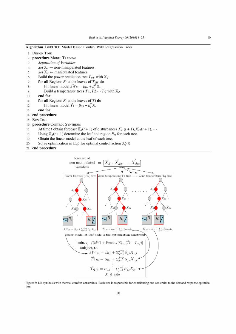
Figure 5: Example of a tree structure obtained using the mbCRT algorithm. The separation of variables allows using the linear model in the leaf touse only control variables.

Figure 4 shows an example of how manipulated and non-manipulated features can get distributed at differentdepths of model based regression tree which uses a linear regression function in the leaves of the tree:

YRi = β0,i + βTi X (3)

Where YRi is the predicted response in region Ri of the tree using all the features X. In such a tree the prediction215

can only be obtained if the values of all the features X’s is known, including the values of the control variables Xci’s.216

Since the manipulated and non-manipulated variables appear in a mixed order in the tree depth, we cannot use this217

tree for control synthesis. This is because the value of the control variables Xci’s is unknown, one cannot navigate to218

any single region using the forecasts of disturbances alone.219

The mbCRT algorithm avoids this problem using a simple but clever idea. We still partition the entire data spaceinto regions using CART algorithm, but the top part of the regression tree is learned only on the non-manipulatedfeatures Xd or disturbances as opposed to all the features X (Figure 5) In every region at the leaves of the “disturbance”tree a linear model is fit but only on the control variables Xc:

YRi = β0,i + βTi Xc (4)

Separation of variables allows us to use the forecast of the disturbances Xd to navigate to the appropriate region Ri220

and use the linear regression model (YRi = β0,i + βTi Xc) with only the control/manipulated features in it as the valid221

prediction model for that time-step.222

9

Behl et al. / Applied Energy 00 (2016) 1–25 10

Algorithm 1 mbCRT: Model Based Control With Regression Trees

1: Design Time2: procedure Model Training3: Separation of Variables4: Set Xc ← non-manipulated features5: Set Xd ← manipulated features6: Build the power prediction tree TkW with Xd

7: for all Regions Ri at the leaves of TkW do8: Fit linear model ˆkWRi = β0,i + βT

i Xc

9: Build q temperature trees T1,T2 · · · Tq with Xd

10: end for11: for all Regions Ri at the leaves of Ti do12: Fit linear model T i = β0,i + βT

i Xc

13: end for14: end procedure15: Run Time16: procedure Control Synthesis17: At time t obtain forecast Xd(t + 1) of disturbances Xd1(t + 1), Xd2(t + 1), · · ·18: Using Xd(t + 1) determine the leaf and region Rrt for each tree.19: Obtain the linear model at the leaf of each tree.20: Solve optimization in Eq5 for optimal control action X∗c(t)21: end procedure

Xd1

Xd2

Xd3

ˆkWRi = β0,i +∑j=p

j=1 βj,iXc,j

R1 Ri

Xd3

Xd1

Xd2

Xd3

R1 Ri

Xd3

Xd1

Xd2

Xd3

R1 Ri

Xd3

T1Ri = α0,i +∑j=p

j=1 αj,iXc,j T qRi = α0,i +∑j=p

j=1 αj,iXc,j

· · · · · ·

forecast ofnon-manipulated

variables= [Xd1, Xd2, · · · Xdm]︸ ︷︷ ︸

Power forecast (kW) tree Zone temperature T1 tree Zone temperature Tq tree· · ·

min.Xcf( ˆkW ) + Penalty[

∑qk=1(Tk − Tref)]

subject toˆkWRi = β0,i +

∑j=pj=1 βj,iXc,j

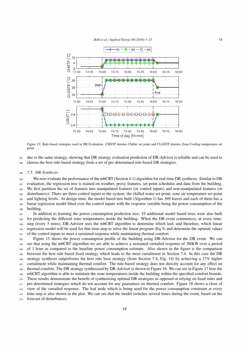
T1Ri = α0,i +∑j=pj=1 αj,iXc,j

T qRi = α0,i +∑j=pj=1 αj,iXc,j

...

Xc ∈ Safe

linear model at leaf node is the optimization constraint

Figure 6: DR synthesis with thermal comfort constraints. Each tree is responsible for contributing one constraint to the demand response optimiza-tion.

10

Behl et al. / Applied Energy 00 (2016) 1–25 11

4.2. DR synthesis optimization223

In the case of DR synthesis for buildings, the response variable is power consumption, the objective function can224

denote the financial reward of minimizing the power consumption during the DR event. However, the curtailment must225

not result in high levels of discomfort for the building occupants. In order to account for thermal comfort, in addition226

to learning the tree for power consumption forecast, we can also learn different trees to predict the temperature of227

different zones in the building. As shown in Figure 6 and Algorithm 1, at each time-step during the DR event, a228

forecast of the non manipulated variables is used by each tree, to navigate to the appropriate leaf node. For the229

power forecast tree, the linear model at the leaf node relates the predicted power consumption of the building to the230

manipulated/control variables i.e., ˆkW = β0,i + βTi Xc.231

Similarly, for each zone 1, 2, · · · q, a tree is built whose response variable is the zone temperature Ti. The linear232

model at the leaf node of each of the zone temperature tree relates the predicted zone temperature to the manipulated233

variables T i = α0, j + βTj Xc. Therefore, at every time-step, based on the forecast of the non-manipulated variables, we234

obtain q + 1 linear models between the power consumption and q zone temperatures and the manipulated variables.235

We can then solve the following DR synthesis optimization problem to obtain the values of the manipulated variables236

Xc:237

minimizeXc

f ( ˆkW) + Penalty[q∑

k=1

(Tk − Tre f )]

subject toˆkW = β0,i + βT

i Xc

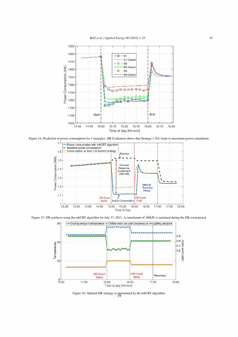
T1 = α0,1 + βT1 Xc

· · ·

T d = α0,q + βTq Xc

Xc ∈ Xsa f e

(5)

The linear model between the response variable YRi and the control features Xc is assumed for computational238

simplicity. Other models could also be used at the leaves as long as they adhere to the separation of variables principle.239

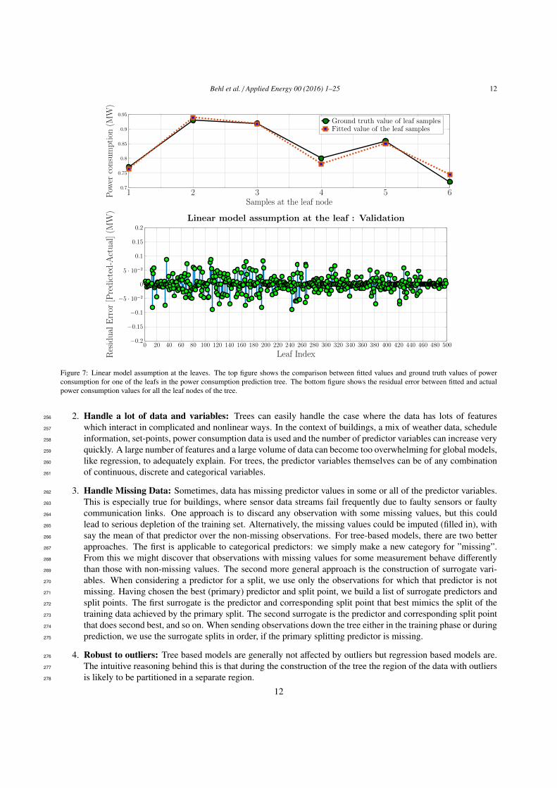
Figure 7 shows that the linear model assumption in the leaves of the tree is a valid assumption.240

The intuition behind the mbCRT Algorithm 1 is that at run time t, we use the forecast Xd(t + 1) of the disturbance241

features to determine the region of the uncontrollable tree and hence, the linear model to be used for the control. We242

then solve the simple linear program corresponding to that region to obtain the optimal values of the control variables.243

The mbCRT algorithm is the first ever algorithm which allows the use of regression trees for control synthesis.244

5. The case for using regression trees for demand response245

Trees share the advantage of being a simple approach, much like other data-driven approaches. However, they246

offer several other advantages in addition to being interpretable, which make them suitable for solving the challenges247

of demand response discussed in Section 2. We list some of these advantages here:248

1. Fast computation times: Trees require very low computation power, both running time and storage require-249

ments. With N observations and p predictors trees require pNlogN operations for an initial sort for each pre-250

dictor, and typically another pNlogN operations for the split computations. If the splits occurred near the edges251

of the predictor ranges, this number can increase to N2 p. Once the tree is built, the time to make predictions is252

extremely fast since obtaining a response prediction is simply a matter of traversing the tree with fixed rules at253

every node. For fast demand response, where the price of electricity could change several times within a few254

minutes, trees can provide very fast predictions.255

11

Behl et al. / Applied Energy 00 (2016) 1–25 12

1 2 3 4 5 60.7

0.75

0.8

0.85

0.9

0.95

Samples at the leaf node

Pow

erconsumption

(MW)

Ground truth value of leaf samplesFitted value of the leaf samples

0 20 40 60 80 100 120 140 160 180 200 220 240 260 280 300 320 340 360 380 400 420 440 460 480 500−0.2

−0.15

−0.1

−5 · 10−2

0

5 · 10−2

0.1

0.15

0.2

Leaf IndexResidual

Error

[Predicted-Actual](M

W)

Linear model assumption at the leaf : Validation

Figure 7: Linear model assumption at the leaves. The top figure shows the comparison between fitted values and ground truth values of powerconsumption for one of the leafs in the power consumption prediction tree. The bottom figure shows the residual error between fitted and actualpower consumption values for all the leaf nodes of the tree.

2. Handle a lot of data and variables: Trees can easily handle the case where the data has lots of features256

which interact in complicated and nonlinear ways. In the context of buildings, a mix of weather data, schedule257

information, set-points, power consumption data is used and the number of predictor variables can increase very258

quickly. A large number of features and a large volume of data can become too overwhelming for global models,259

like regression, to adequately explain. For trees, the predictor variables themselves can be of any combination260

of continuous, discrete and categorical variables.261

3. Handle Missing Data: Sometimes, data has missing predictor values in some or all of the predictor variables.262

This is especially true for buildings, where sensor data streams fail frequently due to faulty sensors or faulty263

communication links. One approach is to discard any observation with some missing values, but this could264

lead to serious depletion of the training set. Alternatively, the missing values could be imputed (filled in), with265

say the mean of that predictor over the non-missing observations. For tree-based models, there are two better266

approaches. The first is applicable to categorical predictors: we simply make a new category for ”missing”.267

From this we might discover that observations with missing values for some measurement behave differently268

than those with non-missing values. The second more general approach is the construction of surrogate vari-269

ables. When considering a predictor for a split, we use only the observations for which that predictor is not270

missing. Having chosen the best (primary) predictor and split point, we build a list of surrogate predictors and271

split points. The first surrogate is the predictor and corresponding split point that best mimics the split of the272

training data achieved by the primary split. The second surrogate is the predictor and corresponding split point273

that does second best, and so on. When sending observations down the tree either in the training phase or during274

prediction, we use the surrogate splits in order, if the primary splitting predictor is missing.275

4. Robust to outliers: Tree based models are generally not affected by outliers but regression based models are.276

The intuitive reasoning behind this is that during the construction of the tree the region of the data with outliers277

is likely to be partitioned in a separate region.278

12

Behl et al. / Applied Energy 00 (2016) 1–25 13

Figure 8: Screenshot of the DR-Advisor MATLAB based GUI.

Figure 9: DR-Advisor Workflow

6. DR-Advisor:Toolbox design279

The algorithms described thus far, have been implemented into a MATLAB based tool called DR-Advisor. We280

have also developed a graphical user interface (GUI) for the tool (Figure 8) to make it user-friendly.281

Starting from just building power consumption and temperature data, the user can leverage all the features of DR-282

Advisor and use it to solve the different DR challenges. The toolbox design follows a simple and efficient workflow283

as shown in Figure 9. Each step in the workflow is associated with a specific tab in the GUI. The workflow is divided284

into the following steps:285

1. Upload Data: When the toolbox loads, the Input tab of the GUI (Figure 8) is displayed. Here the user can286

upload and specify any sensor data from the building which could be correlated to the power consumption. This287

includes historical power consumption data, any known building operation schedules and zone temperature288

data. The tool is also equipped with the capability to pull historical weather data for a building location from289

the web. The user can also specify or upload electricity pricing or utility tariff data. Once the upload process is290

complete the data structure for learning the different tree based models is created internally. The GUI also has291

a small console which is used to display progress, completion and alert messages for each action in the upload292

process.293

13

Behl et al. / Applied Energy 00 (2016) 1–25 14

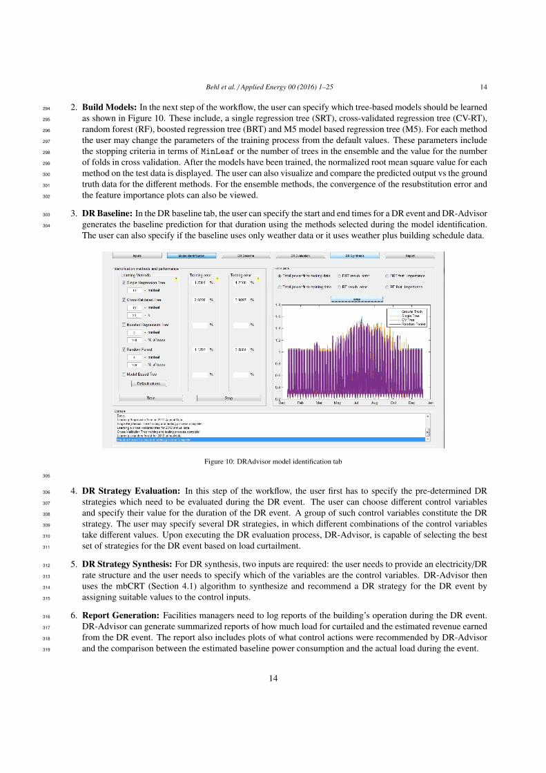
2. Build Models: In the next step of the workflow, the user can specify which tree-based models should be learned294

as shown in Figure 10. These include, a single regression tree (SRT), cross-validated regression tree (CV-RT),295

random forest (RF), boosted regression tree (BRT) and M5 model based regression tree (M5). For each method296

the user may change the parameters of the training process from the default values. These parameters include297

the stopping criteria in terms of MinLeaf or the number of trees in the ensemble and the value for the number298

of folds in cross validation. After the models have been trained, the normalized root mean square value for each299

method on the test data is displayed. The user can also visualize and compare the predicted output vs the ground300

truth data for the different methods. For the ensemble methods, the convergence of the resubstitution error and301

the feature importance plots can also be viewed.302

3. DR Baseline: In the DR baseline tab, the user can specify the start and end times for a DR event and DR-Advisor303

generates the baseline prediction for that duration using the methods selected during the model identification.304

The user can also specify if the baseline uses only weather data or it uses weather plus building schedule data.

Figure 10: DRAdvisor model identification tab

305

4. DR Strategy Evaluation: In this step of the workflow, the user first has to specify the pre-determined DR306

strategies which need to be evaluated during the DR event. The user can choose different control variables307

and specify their value for the duration of the DR event. A group of such control variables constitute the DR308

strategy. The user may specify several DR strategies, in which different combinations of the control variables309

take different values. Upon executing the DR evaluation process, DR-Advisor, is capable of selecting the best310

set of strategies for the DR event based on load curtailment.311

5. DR Strategy Synthesis: For DR synthesis, two inputs are required: the user needs to provide an electricity/DR312

rate structure and the user needs to specify which of the variables are the control variables. DR-Advisor then313

uses the mbCRT (Section 4.1) algorithm to synthesize and recommend a DR strategy for the DR event by314

assigning suitable values to the control inputs.315

6. Report Generation: Facilities managers need to log reports of the building’s operation during the DR event.316

DR-Advisor can generate summarized reports of how much load for curtailed and the estimated revenue earned317

from the DR event. The report also includes plots of what control actions were recommended by DR-Advisor318

and the comparison between the estimated baseline power consumption and the actual load during the event.319

14

Behl et al. / Applied Energy 00 (2016) 1–25 15

Figure 11: 8 different buildings on Penn campus were modeled with DR-Advisor

7. Case study320

DR-Advisor has been developed into a MATLAB toolbox available at http://mlab.seas.upenn.edu/dr-advisor/.321

In this section, we present a comprehensive case study to show how DR-Advisor can be used to address all the afore-322

mentioned demand response challenges (Section 2) and we compare the performance of our tool with other data-driven323

methods.324

7.1. Building description325

We use historical weather and power consumption data from 8 buildings on the Penn campus (Figure 11). These326

buildings are a mix of scientific research labs, administrative buildings, office buildings with lecture halls and bio-327

medical research facilities. The total floor area of the eight buildings is over 1.2 million square feet spanned across.328

The size of each building is shown in Table 1.329

We also use the DoE Commercial Reference Building (DoE CRB) simulated in EnergyPlus [18] as the virtual330

test-bed building. This is a large 12 story office building consisting of 73 zones with a total area of 500, 000 sq ft.331

There are 2, 397 people in the building during peak occupancy. During peak load conditions the building can consume332

up to 1.6 MW of power. For the simulation of the DoE CRB building we use actual meteorological year data from333

Chicago for the years 2012 and 2013. On July 17, 2013, there was a DR event on the PJM ISO grid from 15:00 to334

16:00 hrs. We simulated the DR event for the same interval for the virtual test-bed building.335

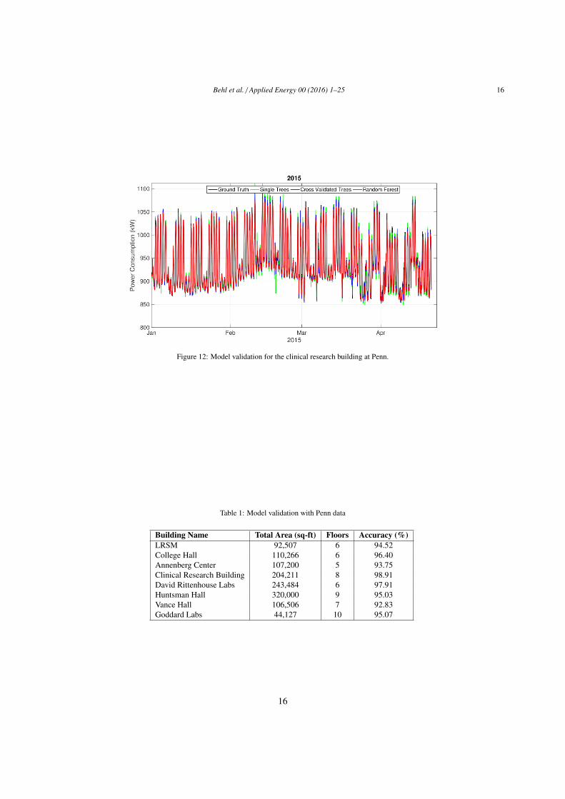
7.2. Model Validation336

For each of the Penn buildings, multiple regression trees were trained on weather and power consumption data337

from August 2013 to December 2014. Only the weather forecasts and proxy variables were used to train the models.338

We then use the DR-Advisor to predict the power consumption in the test period i.e., for several months in 2015. The339

predictions are obtained for each hour, making it equivalent to baseline power consumption estimate. The predictions340

on the test-set are compared to the actual power consumption of the building during the test-set period. One such341

comparison for the clinical reference building is shown in Figure 12. The following algorithms were evaluated: single342

regression tree, k-fold cross validated (CV) trees, boosted regression trees (BRT) and random forests (RF). Our chosen343

metric of prediction accuracy is the one minus the normalized root mean square error (NRMSE). NRMSE is the RMSE344

divided by the mean of the data. The accuracy of the model of all the eight buildings is summarized in Table 1. We345

notice that DR-Advisor performs quite well and the accuracy of the baseline model is between 92.8% to 98.9% for all346

the buildings.347

15

Behl et al. / Applied Energy 00 (2016) 1–25 16

Figure 12: Model validation for the clinical research building at Penn.

Table 1: Model validation with Penn data

Building Name Total Area (sq-ft) Floors Accuracy (%)LRSM 92,507 6 94.52College Hall 110,266 6 96.40Annenberg Center 107,200 5 93.75Clinical Research Building 204,211 8 98.91David Rittenhouse Labs 243,484 6 97.91Huntsman Hall 320,000 9 95.03Vance Hall 106,506 7 92.83Goddard Labs 44,127 10 95.07

16

Behl et al. / Applied Energy 00 (2016) 1–25 17

Table 2: ASHRAE Energy Prediction Competition Results

ASHRAE Team ID WBE CV CHW CV HW CV Average CV9 10.36 13.02 15.24 12.87

DR-Advisor 11.72 14.88 28.13 18.246 11.78 12.97 30.63 18.463 12.79 12.78 30.98 18.852 11.89 13.69 31.65 19.087 13.81 13.63 30.57 19.34

7.3. Energy Prediction Benchmarking348

We compare the performance of DR-Advisor with other data-driven method using a bench-marking data-set from349

the American Society of Heating, Refrigeration and Air Conditioning Engineers (ASHRAE’s) Great Energy Predictor350

Shootout Challenge [19]. The goal of the ASHRAE challenge was to explore and evaluate data-driven models that351

may not have such a strong physical basis, yet that perform well at prediction. The competition attracted ∼ 150352

entrants, who attempted to predict the unseen power loads from weather and solar radiation data using a variety of353

approaches. In addition to predicting the hourly whole building electricity consumption, WBE (kW), both the hourly354

chilled water, CHW (millions of Btu/hr) and hot water consumption, HW (millions of Btu/hr) of the building was355

also required to be a prediction output. Four months of training data with the following features was provided: (a)356

1. Outside temperature (◦F) 2. Wind speed (mph) 3. Humidity ratio (water/dry air) 4. Solar flux (W/m2) In addition to357

these training features, we added three proxy variables of our own: hour of day, IsWeekend and IsHoliday to account358

for correlation of the building outputs with schedule.359

Finally, we use different ensemble methods within DR-Advisor to learn models for predicting the three different360

building attributes. In the actual competition, the winners were selected based on the accuracy of all predictions as361

measured by the normalized root mean square error, also referred to as the coefficient of variation statistic CV. The362

smaller the value of CV, the better the prediction accuracy. ASHRAE released the results of the competition for the363

top 19 entries which they received. In Table 2, we list the performance of the top 5 winners of the competition and364

compare our results with them. It can be seen from table 2, that the random forest implementation in the DR-Advisor365

tool ranks 2nd in terms of WBE CV and the overall average CV. The winner of the competition was an entry from366

David Mackay [20] which used a particular form of bayesian modeling using neural networks.367

The result we obtain clearly demonstrates that the regression tree based approach within DR-Advisor can generate368

predictive performance that is comparable with the ASHRAE competition winners. Furthermore, since regression369

trees are much more interpretable than neural networks, their use for building electricity prediction is, indeed, very370

promising.371

7.4. DR-Evaluation372

We test the performance of 3 different rule based strategies shown in Fig. 13. Each strategy determines the set373

point schedules for chiller water, zone temperature and lighting during the DR event. These strategies were derived374

on the basis of automated DR guidelines provided by Siemens [21]. Chiller water set point is same in Strategy 1 (S1)375

and Strategy 3 (S3), higher than that in Strategy 2 (S2). Lighting level in S3 is higher than in S1 and S2.376

We use auto-regressive trees (Section 3.3) with order, δ = 6 to predict the power consumption for the entire377

duration (1 hour) at the start of DR Event. In addition to learning the tree for power consumption, additional auto-378

regressive trees are also built for predicting the zone temperatures of the building. At every time step, first the zone379

temperatures are predicted using the trees for temperature prediction. Then the power tree uses this temperature380

forecast along with lagged power consumption values to predict the power consumption recursively until the end of381

the prediction horizon.382

Fig. 14 shows the power consumption prediction using the auto-regressive trees and the ground truth obtained383

by simulation of the DoE CRB virtual test-bed for each rule-based strategy. Based on the predicted response, in this384

case DR-Advisor chooses to deploy the strategy S1, since it leads to the least amount of electricity consumption. The385

predicted response due to the chosen strategy aligns well with the ground truth power consumption of the building386

17

Behl et al. / Applied Energy 00 (2016) 1–25 18

Figure 13: Rule-based strategies used in DR Evaluation. CHSTP denotes Chiller set point and CLGSTP denotes Zone Cooling temperature setpoint.

due to the same strategy, showing that DR strategy evaluation prediction of DR-Advisor is reliable and can be used to387

choose the best rule-based strategy from a set of pre-determined rule-based DR strategies.388

7.5. DR-Synthesis389

We now evaluate the performance of the mbCRT (Section 4.1) algorithm for real-time DR synthesis. Similar to DR390

evaluation, the regression tree is trained on weather, proxy features, set-point schedules and data from the building.391

We first partition the set of features into manipulated features (or control inputs) and non-manipulated features (or392

disturbances). There are three control inputs to the system: the chilled water set-point, zone air temperature set-point393

and lighting levels. At design time, the model based tree built (Algorithm 1) has 369 leaves and each of them has a394

linear regression model fitted over the control inputs with the response variable being the power consumption of the395

building.396

In addition to learning the power consumption prediction tree, 19 additional model based trees were also built397

for predicting the different zone temperatures inside the building. When the DR event commences, at every time-398

step (every 5 mins), DR-Advisor uses the mbCRT algorithm to determine which leaf, and therefore, which linear399

regression model will be used for that time-step to solve the linear program (Eq 5) and determine the optimal values400

of the control inputs to meet a sustained response while maintaining thermal comfort.401

Figure 15 shows the power consumption profile of the building using DR-Advisor for the DR event. We can402

see that using the mbCRT algorithm we are able to achieve a sustained curtailed response of 380kW over a period403

of 1 hour as compared to the baseline power consumption estimate. Also shown in the figure is the comparison404

between the best rule based fixed strategy which leads to the most curtailment in Section 7.4. In this case the DR405

strategy synthesis outperforms the best rule base strategy (from Section 7.4, Fig. 14) by achieving a 17% higher406

curtailment while maintaining thermal comfort. The rule-based strategy does not directly account for any effect on407

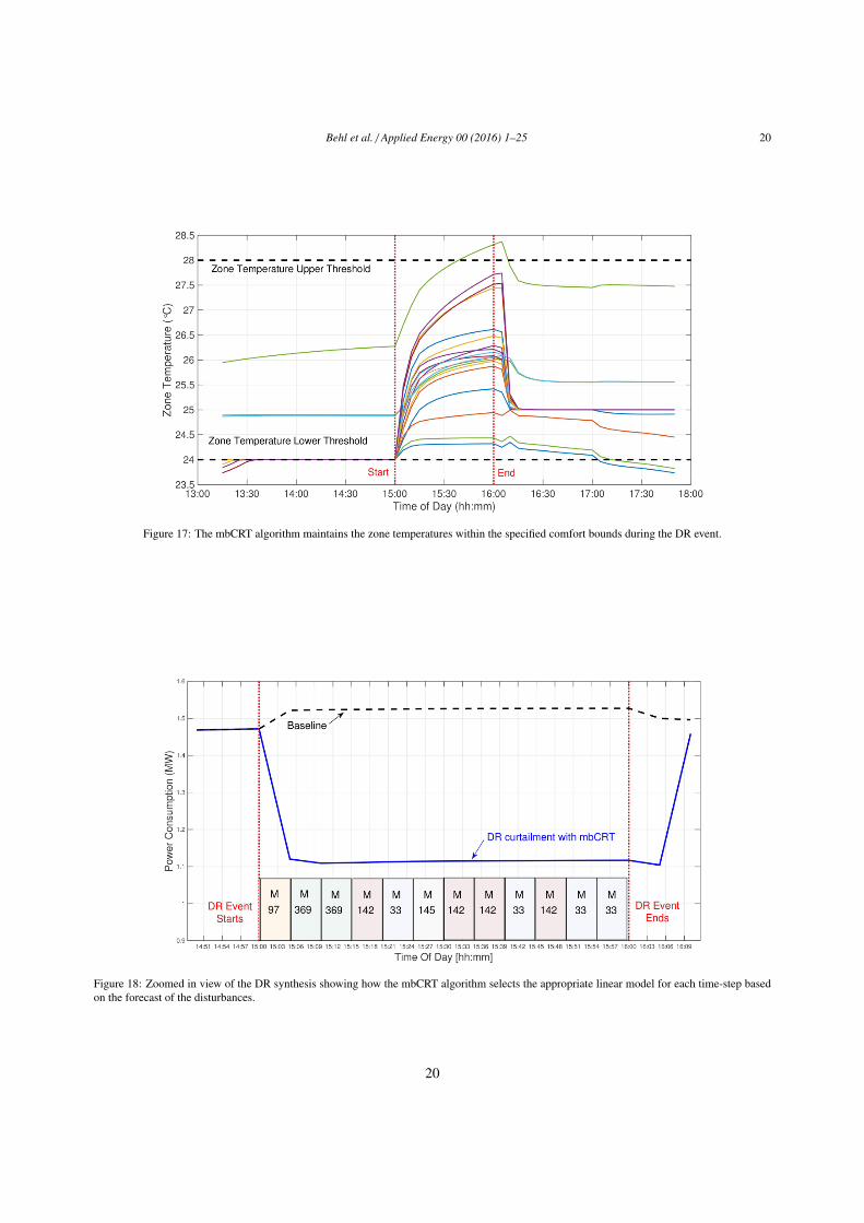
thermal comfort. The DR strategy synthesized by DR-Advisor is shown in Figure 16. We can see in Figure 17 how the408

mbCRT algorithm is able to maintain the zone temperatures inside the building within the specified comfort bounds.409

These results demonstrate the benefit of synthesizing optimal DR strategies as opposed ot relying on fixed rules and410

pre-determined strategies which do not account for any guarantees on thermal comfort. Figure 18 shows a close of411

view of the curtailed response. The leaf node which is being used for the power consumption constraint at every412

time-step is also shown in the plot. We can see that the model switches several times during the event, based on the413

forecast of disturbances.414

18

Behl et al. / Applied Energy 00 (2016) 1–25 19

Figure 14: Prediction of power consumption for 3 strategies. DR Evaluation shows that Strategy 1 (S1) leads to maximum power curtailment.

Figure 15: DR synthesis using the mbCRT algorithm for July 17, 2013. A curtailemnt of 380kW is sustained during the DR event period.

Figure 16: Optimal DR strategy as determined by the mbCRT algorithm.19

Behl et al. / Applied Energy 00 (2016) 1–25 20

Figure 17: The mbCRT algorithm maintains the zone temperatures within the specified comfort bounds during the DR event.

Figure 18: Zoomed in view of the DR synthesis showing how the mbCRT algorithm selects the appropriate linear model for each time-step basedon the forecast of the disturbances.

20

Behl et al. / Applied Energy 00 (2016) 1–25 21

These results show the effectiveness of the mbCRT algorithm to synthesize DR actions in real-time while utilizing415

a simple data-driven tree-based model.416

7.5.1. Revenue from Demand Response417

We use Con Edison utility company’s commercial demand response tariff structure [22] to estimate the financial418

reward obtained due to the curtailment achieved by the DR-Advisor for our Chicago based DoE commercial reference419

building. The utility provides a $25/kW per month as a reservation incentive to participate in the real-time DR420

program for summer. In addition to that, a payment of $1 per kWh of energy curtailed is also paid. For our test-bed,421

the peak load curtailed is 380kW. If we consider ∼ 5 such events per month for 4 months, this amounts to a revenue of422

∼ $45, 600 for participating in DR which is 37.9% of the energy bill of the building for the same duration ($120, 317).423

This is a significant amount, especially since using DR-Advisor does not require an investment in building complex424

modeling or installing sensor retrofits to a building.425

8. Related work426

There is a vast amount of literature ([23, 24, 25, 26]) which addresses the problem demand response under dif-427

ferent pricing schemes. However, the majority of approaches so far have focused either on rule-based approaches for428

curtailment or on model-based approaches, such as the one described in [24]; in which model predictive control is used429

for DR based on a grey-box model of a building. [23] uses a high-fidelity physics based model of the building to solve430

a problem similar to the DR evaluation problem. [26] uses model predictive control for closed-loop optimal control431

strategy for load shifting in a plant that is charged for electricity on both time-of-use and peak demand pricing. One432

of the seminal studies of application of model predictive control on real buildings for demand response and energy-433

efficiency operation came from the Opticontrol project [10]. After several years of work on using grey-box and white434

box models for demand response control design, the authors state that the usefulness of any model based controller435

must be measured by not only its benefits and savings but also its incurred costs, such as the necessary hardware and436

software and the systems design, implementation, and maintenance effort. They further conclude that the biggest hur-437

dle to mass adoption of intelligent building control is the cost and effort required to capture accurate dynamical models438

of the buildings. Since DR-Advisor only learns an aggregate building level model and combined with the fact that439

weather forecasts from third party vendors are expected to become cheaper; there is little to no additional sensor cost440

of implementing the DR-Advisor recommendation system in large buildings. The difficulties in identifying models441

for buildings is also highlighted in [27]. The authors observe that while model creation is mentioned only marginally442

in majority of the academical works dealing with model predictive control, these usually assume that the model of443

the system is either perfectly known or found in literature, the task is much more complicated and time consuming in444

case of a real application and sometimes, it can be even more complex and involved than the controller design itself.445

There are ongoing efforts to make tuning and identifying white box models of buildings more autonomous [11].446

There is recent work, which has explored aspects of modeling, implementation and implications of demand re-447

sponse buildings [28, 29, 30, 31], however, their focus has mainly been on the residential sector. [30] shows that in448

general demand response contributes to a lower cost, higher reliability, and lower emission level of power system449

operation and highlights the societal value of DR. In [31] authors study the short term and long term affects of DR450

on residential electricity consumers through an elaborate empirical study. A reduced order physics based, grey-box451

modeling technique for simulating residential electric demand is presented in [29]. The ability to determine the correct452

response for large commercial buildings (from DR evaluation or DR synthesis) on a fast time scales (1-5 min) using453

purely data-driven methods makes both our approach and tool, novel.454

Several machine learning and data-driven approaches have also been utilized before for forecasting electricity load.455

We already compared the performance of DR-Advisor against several data-driven methods in Section 7.3. In [32],456

seven different machine learning algorithms are applied to a residential data set with the objective of determining457

which techniques are most successful for predicting next hour residential building consumption. [33] uses artificial458

neural networks and regression models for modeling the energy demand of the residential sector in the U.S.. A fore-459

casting method for cooling and electricity load demand is presented in [34], while a statistical analysis of the impact460

of weather on peak electricity demand using actual meteorological data is presented in [35]. In [36] a software archi-461

tecture using parallel computing is presented to support data-driven demand response optimization. The shortcoming462

21

Behl et al. / Applied Energy 00 (2016) 1–25 22

of work in this area is twofold: First, the time-scales at which the forecasts are generated ranges from 15-20 mins to463

hourly forecast; which is too coarse grained for DR events and for real-time price changes. Secondly, the focus in464

these methods is only on load forecasting but not on control synthesis, whereas the mbCRT algorithm presented in465

this paper enables the use of regression trees for control synthesis for the very first time.466

9. Conclusions and ongoing work467

We present a data-driven approach for modeling and control for demand response of large scale energy systems468

which are inherently messy to model using first principles based methods. We show how regression tree based methods469

are well suited to address challenges associated with demand response for large C/I/I consumers while being simple470

and interpretable. We have incorporated all our methods into the DR-Advisor tool - http://mlab.seas.upenn.471

edu/dr-advisor/.472

DR-Advisor achieves a prediction accuracy of 92.8% to 98.9% for eight buildings on the University of Pennsyl-473

vania’s campus. We compare the performance of DR-Advisor on a benchmarking data-set from AHRAE’s energy474

predictor challenge and rank 2nd among the winners of that competition. We show how DR-Advisor can select the475

best rule-based DR strategy, which leads to the most amount of curtailment, from a set of several rule-based strategies.476

We presented a model based control with regression trees (mbCRT) algorithm which enables control synthesis using477

regression tree based structures for the first time. Using the mbCRT algorithm, DR-Advisor can achieve a sustained478

curtailment of 380kW during a DR event. Using a real tariff structure, we estimate a revenue of ∼ $45,600 for the479

DoE reference building over one summer which is 37.9% of the summer energy bill for the building. The mbCRT480

algorithm outperforms even the best rule-based strategy by 17%. DR-Advisor bypasses cost and time prohibitive481

process of building high fidelity models of buildings that use grey and white box modeling approaches while still482

being suitable for control design. These advantages combined with the fact that the tree based methods achieve high483

prediction accuracy, make DR-Advisor an alluring tool for evaluating and planning DR curtailment responses for large484

scale energy systems.485

10. Acknowledgments486

This work was supported in part by STARnet, a Semiconductor Research Corporation program, sponsored by487

MARCO and DARPA and by NSF MRI-0923518 grants.488

References489

[1] J. M. Melillo, T. Richmond, G. W. Yohe, Climate change impacts in the united states: the third national climate assessment, US Global490

change research program 841.491

[2] N. N. C. for Environmental Information, State of the climate: Global analysis for august 2015, [published online September 2015, retrieved492

on October 15, 2015 from http://www.ncdc.noaa.gov/sotc/global/201508.].493

[3] P. I. Michael J. Kormos, Pjm response to consumer reports on 2014 winter pricing.494

[4] C. Goldman, Coordination of energy efficiency and demand response, Lawrence Berkeley National Laboratory.495

[5] F. E. R. Commission, et al., Assessment of demand response and advanced metering.496

[6] P. Interconnection, 2014 deamand response operations markets activity report.497

[7] N. Research, Demand response for commercial & industrial markets market players and dynamics, key technologies, competitive overview,498

and global market forecasts.499

[8] Energy price risk and the sustainability of demand side supply chains, Applied Energy 123 (0) (2014) 327 – 334.500

[9] D. B. Crawley, L. K. Lawrie, et al., Energyplus: creating a new-generation building energy simulation program, Energy and Buildings 33 (4)501

(2001) 319 – 331.502

[10] D. Sturzenegger, D. Gyalistras, M. Morari, R. S. Smith, Model predictive climate control of a swiss office building: Implementation, results,503

and cost-benefit analysis.504

[11] J. R. New, J. Sanyal, M. Bhandari, S. Shrestha, Autotune e+ building energy models, Proceedings of the 5th National SimBuild of IBPSA-505

USA.506

[12] L. Breiman, J. Friedman, C. J. Stone, R. A. Olshen, Classification and regression trees, CRC press, 1984.507

[13] C. Giraud-Carrier, Beyond predictive accuracy: what?, Proceedings of the ECML-98 Workshop on Upgrading Learning to Meta-Level:508

Model Selection and Data Transformation (1998) 78–85.509

[14] L. Breiman, Random forests, Machine learning 45 (1) (2001) 5–32.510

[15] J. Elith, J. R. Leathwick, T. Hastie, A working guide to boosted regression trees, Journal of Animal Ecology 77 (4) (2008) 802–813.511

22

Behl et al. / Applied Energy 00 (2016) 1–25 23

[16] J. R. Quinlan, et al., Learning with continuous classes, in: 5th Australian joint conference on artificial intelligence, Vol. 92, Singapore, 1992,512

pp. 343–348.513

[17] J. H. Friedman, Multivariate adaptive regression splines, The annals of statistics (1991) 1–67.514

[18] M. Deru, K. Field, D. Studer, et al., U.s. department of energy commercial reference building models of the national building stock.515

[19] J. F. Kreider, J. S. Haberl, Predicting hourly building energy use: The great energy predictor shootout–overview and discussion of results,516

Tech. rep., American Society of Heating, Refrigerating and Air-Conditioning Engineers, Inc., Atlanta, GA (United States) (1994).517

[20] D. J. MacKay, et al., Bayesian nonlinear modeling for the prediction competition, ASHRAE transactions 100 (2) (1994) 1053–1062.518

[21] Siemens, Automated demand response using openadr: Application guide (2011).519

[22] Con Edison, Demand response programs details.520

URL http://www.coned.com/energyefficiency/pdf/proposed-program-changes.pdf521

[23] D. Auslander, D. Caramagno, D. Culler, T. Jones, A. Krioukov, M. Sankur, J. Taneja, J. Trager, S. Kiliccote, R. Yin, et al., Deep demand522

response: The case study of the citris building at the university of california-berkeley.523

[24] F. Oldewurtel, D. Sturzenegger, G. Andersson, M. Morari, R. S. Smith, Towards a standardized building assessment for demand response, in:524

Decision and Control (CDC), 2013 IEEE 52nd Annual Conference on, IEEE, 2013, pp. 7083–7088.525

[25] P. Xu, P. Haves, M. A. Piette, J. Braun, Peak demand reduction from pre-cooling with zone temperature reset in an office building, Lawrence526

Berkeley National Laboratory.527

[26] A. J. Van Staden, J. Zhang, X. Xia, A model predictive control strategy for load shifting in a water pumping scheme with maximum demand528

charges, Applied Energy 88 (12) (2011) 4785–4794.529

[27] E. Zacekova, Z. Vana, J. Cigler, Towards the real-life implementation of mpc for an office building: Identification issues, Applied Energy530

135 (2014) 53–62.531

[28] A. Kialashaki, J. R. Reisel, Modeling of the energy demand of the residential sector in the united states using regression models and artificial532

neural networks, Applied Energy 108 (0) (2013) 271 – 280. doi:http://dx.doi.org/10.1016/j.apenergy.2013.03.034.533

URL http://www.sciencedirect.com/science/article/pii/S0306261913002304534

[29] M. Muratori, M. C. Roberts, R. Sioshansi, V. Marano, G. Rizzoni, A highly resolved modeling technique to simulate residential power535

demand, Applied Energy 107 (0) (2013) 465 – 473. doi:http://dx.doi.org/10.1016/j.apenergy.2013.02.057.536

URL http://www.sciencedirect.com/science/article/pii/S030626191300175X537

[30] B. Dupont, K. Dietrich, C. D. Jonghe, A. Ramos, R. Belmans, Impact of residential demand response on power system operation: A belgian538

case study, Applied Energy 122 (0) (2014) 1 – 10. doi:http://dx.doi.org/10.1016/j.apenergy.2014.02.022.539

URL http://www.sciencedirect.com/science/article/pii/S0306261914001585540

[31] C. Bartusch, K. Alvehag, Further exploring the potential of residential demand response programs in electricity distribution, Applied Energy541

125 (0) (2014) 39 – 59. doi:http://dx.doi.org/10.1016/j.apenergy.2014.03.054.542

[32] R. E. Edwards, J. New, L. E. Parker, Predicting future hourly residential electrical consumption: A machine learning case study, Energy and543

Buildings 49 (2012) 591–603.544

[33] A. Kialashaki, J. R. Reisel, Modeling of the energy demand of the residential sector in the united states using regression models and artificial545

neural networks, Applied Energy 108 (2013) 271–280.546

[34] A. Vaghefi, M. Jafari, E. Bisse, Y. Lu, J. Brouwer, Modeling and forecasting of cooling and electricity load demand, Applied Energy 136547

(2014) 186–196.548

[35] T. Hong, W.-K. Chang, H.-W. Lin, A fresh look at weather impact on peak electricity demand and energy use of buildings using 30-year549

actual weather data, Applied Energy 111 (2013) 333–350.550

[36] W. Yin, Y. Simmhan, V. K. Prasanna, Scalable regression tree learning on hadoop using openplanet, in: Proceedings of third international551

workshop on MapReduce and its Applications Date, ACM, 2012, pp. 57–64.552

[37] T. Hastie, R. Tibshirani, J. Friedman, T. Hastie, J. Friedman, R. Tibshirani, The elements of statistical learning, Vol. 2, Springer, 2009.553

[38] B. D. Ripley, Pattern Recognition and Neural Networks, Cambridge University Press, Cambridge, 1996.554

Appendix A. Building regression trees555

We explain how regression trees are built using an example adapted from [37]. Tree-based methods partition thefeature space into a set of rectangles (more formally, hyper-rectangles) and then fit a simple model in each one. Theyare conceptually simple yet powerful. Let us consider a regression problem with continuous response Y and inputsX1 and X2, each taking values in the unit interval. The top left plot of Figure A.19 shows a partition of the featurespace by lines that are parallel to the coordinate axes. In each partition element we can model Y with a differentconstant. However, there is a problem: although each partitioning line has a simple description like X1 = k, someof the resulting regions are complicated to describe. To simplify things, we can restrict ourselves to only considerrecursive binary partitions, like the ones shown in the top right plot of Figure A.19. We first split the space into tworegions, and model the response by the mean of Y in each region. We choose the variable and split-point to achieve thebest prediction of Y . Then one or both of these regions are split into two more regions, and this process is continued,until some stopping rule is applied. This is the recursive partitioning part of the algorithm. For example, in the topright plot of Figure A.19, we first split at X1 = t1. Then the region X1 ≤ t1 is split at X2 = t2 and the region X1 > t1 issplit at X1 = t3. Finally, the region X1 > t3 is split at X2 = t4. The result of this process is a partition of the data-spaceinto the five regions R1,R2, · · · ,R5. The corresponding regression tree model predicts Y with a constant ci in region

23

Behl et al. / Applied Energy 00 (2016) 1–25 24

Figure A.19: Top right: 2D feature space by recursive binary splitting. Top left: partition that cannot be obtained from recursive binary splitting.Bottom left: tree corresponding to the partition. Bottom right: perspective plot of the prediction surface.

Ri i.e.,,

T (X) =

5∑i=1

ciI {(X1, X2) ∈ Ri} (A.1)

This same model can be represented by the binary tree shown in the bottom left of Figure A.19. The full data-set sits556

at the top or the root of the tree. Observations satisfying the condition at each node are assigned to the left branch,557

and the others to the right branch. The terminal nodes or leaves of the tree correspond to the regions R1,R2, ...,R5.558

Appendix A.1. Node splitting criteria559

For regression trees we adopt the sum of squares as our splitting criteria i.e a variable at a node will be split if itminimizes the following sum of squares between the predicted response and the actual output variable.∑

(yi − T (xi))2 (A.2)

It is easy to see that the best response ci (from equation A.1 for yi from partition Ri is just the average of outputsamples in the region Ri i.e

ci = avg(yi|xi ∈ Ri) (A.3)

Finding the best binary partition in terms of minimum sum of squares is generally computationally infeasible. Agreedy algorithm is used instead. Starting with all of the data, consider a splitting variable j and split point s, anddefine the following pair of left (RL) and right (RR) half-planes

RL( j, s) ={X|X j ≤ s

},

RR( j, s) ={X|X j > s

} (A.4)

The splitting variable j and the split point s is obtained by solving the following minimization:

minj,s

mincL

∑xi∈RL( j,s)

(yi − cL)2 + mincR

∑xi∈RR( j,s)

(yi − cR)2

(A.5)

24

Behl et al. / Applied Energy 00 (2016) 1–25 25

where, for any choice of j and s, the inner minimization in equation A.5 is solved using

cL = avg(yi|xi ∈ RL( j, s))cR = avg(yi|xi ∈ RR( j, s))

(A.6)

For each splitting variable X j, the determination of the split point s can be done very quickly and hence by scanning560

through all of the inputs (Xi’s), the determination of the best pair ( j, s) is feasible. Having found the best split, we561

partition the data into the two resulting regions and repeat the splitting process on each of the two regions. Then this562

process is repeated on all of the resulting regions.563

Rather than splitting each node into just two regions at each stage, we might consider multiway splits into more564

than two groups. While this can sometimes be useful, it is not a good general strategy. The problem is that multiway565

splits fragment the data too quickly, leaving insufficient data at the next level down. Hence we would want to use such566

splits only when needed. Also multiway splits can be achieved by a series of binary splits.567

Appendix A.2. Stopping criteria and pruning568

Every recursive algorithm needs to know when it’s done, i.e it requires a stopping criteria. For regression trees this569

means when to stop splitting the nodes. A very large tree might over fit the data, while a small tree might not capture570

the important structure. Tree size is a tuning parameter governing the models complexity, and the optimal tree size571

should be adaptively chosen from the data. One approach is to split tree nodes only if the decrease in sum-of-squares572

due to the split exceeds some threshold. However, this strategy is myopic, since a seemingly worthless split might573

lead to a very good split below it. A preferred, strategy is to grow a large tree, stopping the splitting process only574

when some minimum number of data points at a node (MinLeaf) is reached. Then this large tree is pruned using575

cost-complexity pruning methods.576

Define a subtree T ⊂ T0 to be any tree that can be obtained by pruning T0, i.e. collapsing any number of itsnon-terminal nodes. Let node i corresponding to the partition Ri. |T | denotes the number of terminal nodes in TDefine,

Ni = # {xi ∈ Ri} ,

ci =1Ni

∑xi∈Ri

yi,

Qi(T ) =1Ni

∑xi∈Ri

(yi − ci)2

(A.7)

where Ni is the number of samples in the partition Ri, ci is the estimate of y within Ri and Qi(T ) is the mean squareerror of the estimate ci. The cost complexity criteria is then defined as:

Cα(T ) =

|T |∑i=1

NiQi(T ) + α|T | (A.8)

The goal is to find, for each α, the subtree Tα ⊂ T0 to minimize Cα(T ). The tuning parameter α ≥ 0 governs the trade577

off between tree size and its goodness of fit to the data. For each α one can show that there is a unique smallest subtree578

Tα that minimizes Cα(T ) [38]. Estimation of α is achieved by cross-validation.579

25