Dr. AbediniDr. Abedini

Inventory analysisInventory analysis Space and money prevent companies from Space and money prevent companies from

producing goodsproducing goods

Total CostTotal Cost= = Pc+Cc+OcPc+Cc+Oc

WhereWhere• PcPc= Purchasing Cost per year= Purchasing Cost per year• CcCc=Carrying or Holding Cost per year=Carrying or Holding Cost per year• OcOc= Ordering Cost per year= Ordering Cost per year

CC= $Cost/unit= $Cost/unit DD= Annual demand= Annual demand HH=$Holding cost/unit/year =$Holding cost/unit/year

(Based on Annual Demand)(Based on Annual Demand) QQ= Order Quantity= Order Quantity PP= $Ordering cost/order/year= $Ordering cost/order/year RR= Reorder Point (quantities)= Reorder Point (quantities) Total CostTotal Cost= (C)(D)+H(Q/2)+P(D/Q)= (C)(D)+H(Q/2)+P(D/Q) dTC/dQ = (0)+H/2 – PD/QdTC/dQ = (0)+H/2 – PD/Q Therefore Q*= √(2DP/H)Therefore Q*= √(2DP/H) Q*= Economic Order QuantityQ*= Economic Order Quantity

R=Lead timeR=Lead time Q*= Economic ordering quantityQ*= Economic ordering quantity

• (How many to order)(How many to order)

T= TimeT= Time

C= $10/unitC= $10/unit D= 365,000D= 365,000 H= $5/unit/year (based on demand)H= $5/unit/year (based on demand) P= $500P= $500 Q*=√[2(365,000)(500)/5] = 8544Q*=√[2(365,000)(500)/5] = 8544

(# of units per order)(# of units per order) 365,000/8544 = 42.7365,000/8544 = 42.7 (times in year you order)(times in year you order)

Total cost of carrying inventory=Total cost of carrying inventory= 10(365,000)+5(8544/2)+500(365,000/8544)10(365,000)+5(8544/2)+500(365,000/8544) 3650000+21360+213603650000+21360+21360 $3,692,720.02$3,692,720.02 Under these conditions we assume that the Under these conditions we assume that the

demand is constant and the lead time is demand is constant and the lead time is constant constant

This is known as This is known as Simple E.O.Q.Simple E.O.Q.

% of quantity ordered that can be % of quantity ordered that can be supplied from the available stocksupplied from the available stock

Ex.) Ex.) You want 100 parts but the company You want 100 parts but the company

has only 90 has only 90 Service Level = 90%Service Level = 90%

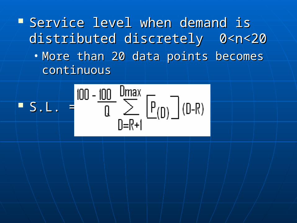
Service level when demand is Service level when demand is distributed discretely 0<n<20distributed discretely 0<n<20• More than 20 data points becomes More than 20 data points becomes

continuouscontinuous

S.L. = S.L. =

DD PP

11 .01.01

22 .04.04

33 .10.10

44 .20.20

55 .30.30

66 .20.20

77 .10.10

88 .04.04

99 .01.01

ReorderReorder SSSS SLSL

55 00 .30.30 .35.35 .2(1)+.1.2(1)+.1 88.8%88.8%

66 11 .20.20 .15.15

77 22 .10.10 .05.05

88 33 .04.04 .01.01

99 44 .01.01 00

Probability that you run out of stock Probability that you run out of stock before you receive your new orderbefore you receive your new order

With uncertain demand With uncertain demand (Continuous distribution)(Continuous distribution)

Now you don’t know when you will run outNow you don’t know when you will run out

Z = X- µ/ Z = X- µ/ σσ µ= 1000/dayµ= 1000/day σσ = 100/ day = 100/ day

σσσσ

RememberRemember

If you an 84 % service level then you If you an 84 % service level then you would just add 1 standard deviationwould just add 1 standard deviation

If you want a 97 % service level then If you want a 97 % service level then you add 2 standard deviationsyou add 2 standard deviations

84% = 1000+100 = 110084% = 1000+100 = 1100 97% = 1000+2(100) = 120097% = 1000+2(100) = 1200

Annual Demand = 365,000Annual Demand = 365,000 Daily Demand = 1000 units/dayDaily Demand = 1000 units/day P = $50 / orderP = $50 / order H = $1.25 / unit / yearH = $1.25 / unit / year L = 9 daysL = 9 days C = $12.50 / unitC = $12.50 / unit SL = 95 % SL = 95 % σσ = 1000 units / day = 1000 units / day Z = 1.64Z = 1.64

SS = ZSS = Zσ√σ√(L)(L) = 1.64(100) = 1.64(100) √√(9)(9) = = 492 Units492 Units

R = DL + SSR = DL + SS = (1000)9 + 492= (1000)9 + 492 = = 9492 Units9492 Units This is when you reorderThis is when you reorder

Q* = Q*= √(2DP/H) Q* = Q*= √(2DP/H) = √[2(365,000)(50)]/ 1.25= √[2(365,000)(50)]/ 1.25 = = 5,404 Units5,404 Units

This is the number of units you This is the number of units you should order during reorder timeshould order during reorder time

Priority rulesPriority rules 1.) First come first serve1.) First come first serve 2.) Shortest processing time (SPT)2.) Shortest processing time (SPT) 3.) Earliest due dates (EDD)3.) Earliest due dates (EDD)

• Prioritize as what is due nextPrioritize as what is due next

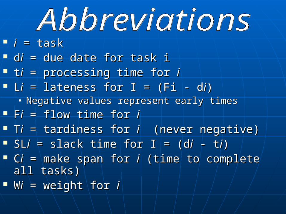
ii = task = task ddii = due date for task i = due date for task i ttii = processing time for = processing time for ii LLii = lateness for I = (Fi - d = lateness for I = (Fi - dii))

• Negative values represent early timesNegative values represent early times FFii = flow time for = flow time for ii TTii = tardiness for = tardiness for ii (never negative) (never negative) SLSLii = slack time for I = (d = slack time for I = (dii - t - tii)) CCii = make span for = make span for ii (time to complete all (time to complete all

tasks)tasks) WWii = weight for = weight for ii

Scheduling Scheduling nn tasks to tasks to 11 processor processor

Rule 1: minimize the average flow time by Rule 1: minimize the average flow time by sequencing in the order of (SPT)sequencing in the order of (SPT)

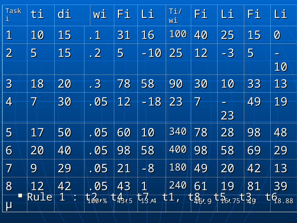
Rule 1 : t2, t4, t7, t1, t8, t5, t3, t6Rule 1 : t2, t4, t7, t1, t8, t5, t3, t6

Task Task ii titi didi wiwi FiFi LiLi Ti/wiTi/wi Fi Fi LiLi FiFi LiLi

11 1010 1515 .1.1 3131 1616 100100 4040 2525 1515 00

22 55 1515 .2.2 55 -10-10 2525 1212 -3-3 55 -10-10

33 1818 2020 .3.3 7878 5858 9090 3030 1010 3333 1313

44 77 3030 .05.05 1212 -18-18 2323 77 -23-23 4949 1919

55 1717 5050 .05.05 6060 1010 340340 7878 2828 9898 4848

66 2020 4040 .05.05 9898 5858 400400 9898 5858 6969 2929

77 99 2929 .05.05 2121 -8-8 180180 4949 2020 4242 1313

88 1212 4242 .05.05 4343 11 240240 6161 1919 8181 3939

µµ 100 %100 % 43.543.5 13.413.4 46.946.9 16.7516.75 4949 18.8818.88

List ActivitiesList Activities Set PrecedenceSet Precedence Compute each crash timeCompute each crash time Design networkDesign network Compute early start timesCompute early start times Compute late finish timesCompute late finish times Design critical pathDesign critical path Compute project costCompute project cost Crash one activityCrash one activity IterateIterate

Critical path – Critical path – Occurs when early start times equal Occurs when early start times equal

late finisheslate finishes

Project evaluation and review Project evaluation and review techniquetechnique

Use expected values rather than Use expected values rather than estimated valuesestimated values