DPSim Modelling: Dynamic Optimization in Large Scale Simulation Models*

RICHARD T. WOODWARD, YONG-SUHK WUI, AND WADE L. GRIFFIN

to appear in

Applications of Simulation Methods in Environmental and Resource Economics

Edited by Anna Alberini and Riccardo Scarpa

Abstract for Proposal:

Although it is well established that dynamically optimal policies should be “closed loop”

so that policies take into account changing conditions of a system, it is rare for such

optimization to actually be carried out in large-scale simulation models. Computational

limitations remain a major barrier to the study of dynamically optimal policies. Since the

size of dynamic optimization problems grows approximately geometrically with the state

* This paper draws extensively on Woodward, Richard T., Yong-Suhk Wui, and Wade L.

Griffin, forthcoming, “Living With The Curse Of Dimensionality: Closed-Loop

Optimization In A Large-Scale Fisheries Simulation Model” American Journal of

Agricultural Economics (forthcoming). Permission has been granted for this purpose

by the American Agricultural Economics Association. We acknowledge valuable

editorial assistance by Michele Zinn and many helpful comments from Bill

Provencher.

1

space, this problem will continue to inhibit the identification of dynamically optimal

policies for the foreseeable future. In this chapter, we explore in detail the problem of

solving dynamic optimization problems for large-scale simulation models and consider

methods to work around the computational barriers. We show that a reasonable approach

is to solve a small-scale problem to identify an approximate value function that can then

be imbedded directly in the simulation model to find approximately optimal time-paths.

We present and compare two ways to specify the small-scale problem: a traditional

“meta-modelling” approach, and a new “direct approach” in which the simulation model

is imbedded directly in the dynamic optimization algorithm. The methods are employed

in a model of the Gulf of Mexico's red snapper fishery and used to identify the

dynamically optimal total allowable catch for the recreational and commercial sectors of

the fishery.

2

I. Introduction

As the chapters in this book demonstrate, simulation modelling is a critical tool

for applied economic analysis. This is particularly true when interdisciplinary analysis is

to be carried out. Natural systems are complicated, and although economists may be

comfortable with general specifications of the physical characteristics of such systems,

the best available models are often quite detailed, representing the system using many

variables and empirically estimated relationships. This presents an important challenge.

If a large simulation model is to be used, in which the state of the system is represented

by dozens if not hundreds of variables, then it is computationally impossible for the

analyst to identify dynamically optimal policy paths. In this chapter we explore means

by which (approximate) dynamically optimal paths can be found, even for very large

simulation models.

This paper is tied closely to Woodward, Wui and Griffin (forthcoming, hereafter

WWG) in which we spell out the problem of carrying out dynamically optimal policy

analysis when working with a large scale simulation model, what we will call DPSim

analysis. In that paper we propose a new way of solving such problems, which we call

the direct approach. In the direct approach the complete simulation model is imbedded

in the dynamic programming algorithm. This is distinguished from the meta-modelling

approach, in which a system of equations is estimated that, in effect, simulate the

simulation model itself. We were unable to find any analysts that had applied the direct

approach previously, while the meta-modelling approach is frequently used.

3

In this chapter we implement and compare the direct and meta-modelling

approaches. Although we cannot draw general conclusions as to which method might be

preferred, in our application the direct approach seems to be preferred, yielding a better

approximation of the simulated system and, therefore, is probably preferred for dynamic

policy analysis.

The chapter is organized as follows. In the next section we spell out the difficulty

and importance of conducting DPSim analysis. Section 2 summarizes two approaches

that can be used to carry out DPSim analysis. The following section discusses our

empirical application and discusses how the two approaches were implemented in this

case. The results of our modelling are presented and the direct and meta-modelling

approaches are compared. The conclusion summarizes our findings and discusses issues

that require further research.

II. The need for and difficulty of dynamic optimization in large scale simulation

models

Simulation modelling plays an important role in policy analysis. However, except

for extremely small and simple models, it is computationally impossible to analyze all

possible policy paths that might be pursued. Hence, truly optimal policy paths cannot be

identified. This is an important limitation for simulation modelers since many policies

have important dynamic consequences, affecting both future consequences and future

options. To the extent that simulation modelling can assist in identifying preferred

policies, it is certainly desirable that dynamically optimal policies be presented.

4

The standard approach to solving empirical dynamic optimization problems is

numerical dynamic programming (DP) (Kennedy, Bertsekas). In such problems, the state

of the system is defined by a vector of state variables, x. Under fairly general conditions,

almost any dynamic optimization problem can be solved to yield an optimal policy rule,

z*(x), and an optimal value function, v(x). Assuming an infinite horizon,1 the value

function is defined implicitly by the Bellman’s equation,

( ) ( ) ( )( )

( )1

1

max ,

. . ,

t t tz

t t t

v x E u x z v x

s t x g x z

β +

+

= +

∼

t (1)

where u(⋅) defines the benefits in the current period as a function of x and choices, z; g(⋅)

defines the conditional probability distribution over future states, xt+1; E is the expectation

operator; and β is the discount factor.2

If the function v(x) were known then, starting at a known initial state, x0, an

optimal policy path could be simulated by successively solving the problem

( ) ( ) ( )( )*1arg max ,t t t

zz x E u x z v xβ += + t

. (2)

1 All of our analysis below is also applicable to finite horizon problems. We present the

infinite horizon case because it is notationally cleaner.

2 In our empirical analysis we use an annual discount rate of seven percent as specified in

Executive Office of the President.

5

In the traditional simulation analysis, a policy rule (frequently expressed as a constant

policy) is simulated for a number of periods. Simulating an optimal path has advantages

both normatively and positively. From a normative perspective, policies that follow a

dynamically optimal policy path will tend to yield greater net benefits. From a positive

perspective, simulating a dynamically optimal path frequently makes more sense because

decision makers do adjust over time to changing conditions. Hence, (2) provides a

preferred foundation for policy simulation.

As noted by WWG, if v(x) were known, then the optimal paths could be simulated

by repeatedly solving (2) with the complete simulation model used to simulate the

optimal policy path. For simulation analysis, therefore, the goal of a DP exercise should

not be to find the optimal policy function, z*(x), but to find an approximate value

function, v(⋅). Once this function is known, an approximately optimal policy path can be

found by including the full simulation model in the policy optimization problem, (2). In

this manner, dynamically optimal analysis can be carried out without abandoning the

large simulation model. We call this approach, which combines simulation analysis with

dynamic optimization, DPSim modelling.

The challenge of DPSim modelling is, of course, that the value function is not

known a priori. In principle v(⋅) can be found using the methods of numerical DP. In

practice, however, it can only be identified for relatively small systems. Regardless of

the solution method employed, solving DP problems requires that a separate optimization

problem be solved at a large number of points in the state space. Hence, the

computational size of a dynamic optimization problem tends to grow exponentially with

6

the number of state variables; a fact that Bellman referred to as the “curse of

dimensionality”. Suppose that there are nx variables in the state space and that each of

these is represented by m different values. In this case, to solve the DP problem m

different optimization problems would need to be solved repeatedly. If nx increases by

one, the size of the problem grows m-fold.

xn

Because of the curse of dimensionality, dynamic optimization problems are

almost always solved only for relatively small systems: nx<10, and usually less than 3.

Certainly DP problems cannot be solved for the large systems in which 100 or more

variables are used to replicate complicated dynamic systems. Although enormous

improvements in the computational speed have been achieved in recent years, this

computational burden will continue to limit the size of DP problems for many years to

come. “Moore’s law” is the regular tendency for the density of computer circuitry (and

processor speed) to double every eighteen months (Schaller). This “law”, which has held

up surprisingly well since its conception in 1965, has startling implications for simulation

modelers: a simulation model could double in size every 1.5 years without slowing down.

The implications for DP, however, are not nearly so promising. For example, in a model

in which each state variable takes on just 8 possible values, it would be 4.5 years before

just one state variable could be added without increasing the run time of the program.

7

The solution of DP problems with hundreds of state variables lies only in the far distant

future.3

III. Two approaches to DPSim modelling

We describe here two ways in which to work within the computational limits to

solve a dynamic optimization problem linked to a large simulation model. To formalize

our discussion we need to introduce some notation. Let Xt be the (large) vector of state

variables used in the simulation model and Zt be a vector of policy options. A policy path

is denoted 0 1, ,...Z=Z Z , where Zt is the vector of policies implemented in period t.

The simulation model can be thought of as a pair of mappings S1 and S2 from choices and

conditions in period t, Zt and Xt, into future conditions, Xt+1, and net benefits in t, ut,

respectively.

{ }

To illuminate the general discussion, in this section we will frequently refer to our

case study that we examine in detail below. Our case study is a fisheries management

problem in which we use the General Bioeconomic Fishery Simulation Model (GBFSM)

as our model foundation. GBFSM is a highly detailed model that has been parameterized

3 Of course brute computational force is not the only option available to the analyst.

Improvements in the efficiency of DP algorithms (e.g., Judd and Mrkaic) and

opportunities exist for very efficient programming including the use of parallel

processors (Rust, 1997b) or Rust’s randomization approach (1997a), which can avoid

the geometric growth in some problems.

8

for the Gulf of Mexico’s red snapper fishery. In the model, red snapper stocks fall into

360 different cohorts distributed across two depth zones (depths 2 and 3 in the model) for

a total of 720 depth-cohort groups. Hence, the complete vector of state variables, Xt

would include 720 elements. One of the policies being considered in the case study is the

total allowable catch (TAC) of red snapper, so that Zt is the TAC chosen. A run of

GBFSM for a single year takes a starting stock, Xt, and a specified TAC level, Zt, and

yields a prediction of the stock in the following year, Xt+1, and the producer and consumer

surplus generated by the fishery, ut.

In general, if in each period there are nz possible policies, then the total number of

possible paths over T periods is . Since Nz grows exponentially in T, for all but

extremely simple or short-run cases it is computationally infeasible to evaluate every

possible policy path. Hence, in most simulation exercises only a small subset of all

possible policy paths are evaluated. Instead of simply optimizing over this extremely

large set of policy paths, it is usually better to solve for v(⋅) in (1).

Tz zN n=

As we noted above, since DP problems with hundreds of state variables cannot be

solved, the alternative way to identify approximate solutions to the DP problem is for the

complete simulation model is to specify an approximating DP problem in terms of a

small set of variables, x, that approximate the complete set in X. The problem of

identifying an approximating value function for a simulation model is presented

graphically in Figure 1 (taken from WWG). For simplicity, we present the model as if it

is deterministic and references to Z and S2 are suppressed to focus on the dynamic

processes of the system, S1.

9

The top half of Figure 1 presents the dynamics of the state variables in the

simulation model while the bottom half of the figure represents a smaller set of state

variables, x, which are used in the DP specification to approximate X. Let x∈x⊂ be a

vector of state variables chosen so that the approximating problem can be solved in a

“reasonable” length of time while still capturing critical features of the simulation model.

In our example, the vector x consists of aggregate stocks of juvenile and adult stocks.

The vector-valued function A:X→x, maps from the full set of state variables into the

small set of variables. As in our example, where A simply adds up the young and adult

fish, the function A typically takes the form of a linear aggregation or average. For each

vector X∈X there is a single vector x=A(X). However, the converse is not true – there

might be an infinite number of vectors X that could give rise to a particular vector x.

Hence, f(x) defines not a single vector X, but a set of vectors that might have given rise to

x and the probability density function over that set. We say that X∈f(x) if A(X)=x.

n

)1 1 ,

To identify the approximate value function, v(x), a DP problem in the space of the

aggregate state variables, x, must be solved. For our example, v(x) is the fishery’s value

as a function of the aggregate stocks. Finding this function requires the mappings s1,

from (xt,Zt) to xt+1, and s2, from (xt,Zt) to ut. As shown in the Figure 1, the true mapping s1

involves three steps: from xt to Xt, then from Xt and Zt to Xt+1 through S1, and finally from

Xt+1 to xt+1, i.e., ( ) ( )(,t t t ts x Z A S f x Z = . As we have noted, however, the mapping

A is many-to-one. Hence, even if X1 and X2∈f(x), the vectors can differ so that

S1(X1,Z)≠S1(X2,Z). Hence, like f(x), the composite mapping s ⋅ is also a mapping into a ( )1

10

probability space; given any value of xt and a choice vector Zt, there is a distribution of

values for xt+1 that might result.4

The challenge of DPSim analysis, therefore, is the development of representations

of simulation models to approximate the composite mappings s1 and s2. Regardless of

how this is done, it is clear that the DP model is stochastic; this is true even if the

simulation model itself is deterministic. In general, the functions s1 and s2 can be

deterministic only in the unlikely case A-1(x) exists.

There are two basic approaches that might be used to capture s1 and s2. Both

approaches have in common that they begin by carrying out a wide range of simulation

runs to generate observations of X that are used as “data”. The traditional approach,

which we call the “meta-modelling” approach, approximates the mappings s1 and s2 using

postulated functional forms, say ˆ ,t ts x Z and ˆ ,t ts x Z . For example, xt+1 might be

predicted using a set of possibly high-order polynomials of xt and Zt. In the meta-

modelling approach the coefficients of ( )1s ⋅ and ( )2s ⋅ are econometrically estimated

using the “data” and these functions are then used to solve the DP problem. In our case

study, therefore, the meta-model allows us to predict future aggregate stocks based on

current aggregate stocks and the TAC level. This approach, represented by the dotted

lines in Figure 1, has been applied by many researchers such as Bryant, Mjelde and

( )1 ( )2

4 The argument would also hold for s2 and ut.

11

Lacewell , Önal et al., Watkins, Lu and Huang, and van Kooten, Young and

Krautkraemer.

In a meta-modelling specification, the simulation model is bypassed entirely once

and are found. In the alternative, which we call the direct approach, the

large simulation model is used directly in the course of solving the DP problem. To

accomplish this, it is necessary to approximate the correspondence f, i.e. the arrow up

from xt to Xt in Figure 1. This provides a means by which to approximate the full vector

of state variables Xt so that the large simulation model can be used directly to predict Xt+1

and ut.

( )1 ( )2s ⋅ s ⋅

In the direct approach the “data” generated from the simulation model are

interpreted as observations of the joint probability distribution of Xt and xt and

econometric methods are used to estimate the one-to-many mapping f. Once the mapping

f is approximated, the direct approach involves three steps. First, given a value of xt, the

disaggregate vector Xt is predicted. Then the large simulation model is run to obtain an

Xt+1 and ut. Finally, using the aggregation function A, xt+1 is found as A(Xt+1). In our case

study these three steps are: 1) the 720 cohort-depth groups are predicted based on the

aggregate stocks in xt; 2) GBFSM is run incorporating at TAC policy, yielding a value of

consumer and producer surplus and the cohort-depth groups in t+1, Xt+1; and 3) the stocks

are aggregated, yielding, xt+1, a prediction of the next-period’s aggregate young and old

fish stocks. This three-step process is repeated numerous times following standard

Monte Carlo methods to obtain the distribution of ut and xt+1, which are then used in the

12

standard way to solve the DP problem.

Although either the meta-modelling approach or the direct approach might be

employed to solve the DPSim problem, neither approach will exactly solve the true DP

problem. Both models find an approximate value function, v(xt), which calculates the

value of the system as a function of the aggregate variables xt instead of the true value

function, which would be a function of Xt. Estimation errors are introduced because the

simulation model is based on X, while the DP model is solved based on x. The meta-

modelling approach introduces errors in the use of functional forms to approximate the

complete mappings s1 and s2. The direct method introduces errors in the prediction of Xt.

It is not possible to rank the two methods a priori. What we can say is that the meta-

modelling approach will have a clear advantage in terms of computational speed since it

only has to evaluate the small set of functions incorporated in and . In the remainder

of this chapter we present our case study in more detail and use it to compare the two

methods.

1 2s s

IV. An empirical application of DPSim analysis: The Gulf of Mexico Red Snapper

Fishery

A. The policy setting

Our empirical application of the methods outlined is for the red snapper fishery of

the Gulf of Mexico. This fishery is an important economic asset: commercial harvests of

red snapper were valued at nearly $12.0 million from 5.08 million pounds in 2000 (U.S.

Department of Commerce) and recreational harvests in the same year were estimated at

13

4.15 million pounds (Gulf of Mexico Fishery Management Council).

The two policy variables we consider here are the total allowable catch (TAC) for

the red snapper fishery, ZT, and the distribution of the TAC between the commercial and

recreational sectors, ZD. The TAC is a fundamentally dynamic choice variable.

Reducing the TAC is essentially an investment decision: benefits today are foregone to

increase the value of the fishery in the future. The value of this investment depends not

only on biological factors, but also on the extent to which future policies respond to

changes in the stock. Dynamic optimization is, therefore, essential to the identification of

the appropriate TAC policies.

To some degree, the need for a dynamically optimal policy has been recognized

by the Gulf of Mexico Fishery Management Council’s (GOMFMC) in their plan to

rebuild the red snapper fishery. The management alternatives evaluated by the Council

call for re-evaluation of the policies every five years based on updated indicators of the

fishery’s health. Although the management alternatives considered by the Council are

somewhat more rigid and limited than might be desirable under a dynamically optimal

policy, it appears that they will react to the changing conditions over time.

B. The simulation model: GBFSM

The simulation model that is at the heart of our analysis is the General

Bioeconomic Fishery Simulation Model (GBFSM). GBFSM permits a high degree of

flexibility, allowing for multiple species, depths, areas, cohorts, fishing vessels, and

more. The model was originally developed to predict how alternative management

14

policies would affect fisheries (Grant, Isaakson, and Griffin) and has been used

extensively for analyzing the effects of management policies in the Gulf of Mexico

(Blomo et al., ; Grant and Griffin; Griffin and Stoll; Griffin and Oliver; Griffin et al.;

Gillig, Griffin, and Ozuna). GBFSM consists of two main parts: a biological submodel

and an economic submodel. The biological submodel represents the recruitment, growth,

movement, and natural and fishing mortality of shrimp and finfish. The economic

submodel, which includes a harvesting sector and a policy sector, represents the monetary

and industry impact. Entry and exit in the commercial sector follow the standard

bioeconomic approach based on economic rents. Recreational effort is predicted using

econometrically estimated recreation-demand functions (Gillig, Griffin, and Ozuna). The

model is parameterized using coefficients from the literature, econometrically estimated

functions, and calibration so that to the greatest extent possible the model replicates

historical trends in the fishery.5

Forty GBFSM simulations were run, each for fifty years. This yielded 2,000

annual observations that were treated as data to estimate parameters for the direct and

meta-modelling approaches. We also used these data to determine the relevant range for

5 There are many details that are suppressed here. A detailed description of GBFSM and

its calibration are available at http://gbfsm.tamu.edu. The discount rate used in the

analysis is the federally mandated rate of 7% per annum (Executive Office of the

President).

15

the simulations, so that the only values for the aggregate state variables were those that

were in the neighborhood of values that were actually observed in the simulations.

C. Solving the DP problem: The direct method

The direct approach requires estimation of functions mapping a state-vector, x,

into a vector of states for the full set of state variables in the simulation model. Three

aggregate variables are used: the recreational catch per day of effort (CPUE) in the

previous year, xc, and the stocks at the beginning of the year of young red snapper (2-

years old or less), xy, and adult red snapper (3-years old and above), xa. The CPUE

variable, xc, coincides exactly with a variable in the simulation model so that a one-to-one

mapping is possible for this variable. For the population variables, however, the size of

the array X is much larger than could be incorporated into a DP model. The red snapper

population in GBFSM is composed 720 depth-cohort groups. Using the simulated data, a

conditional expectation function was estimated for each depth-cohort combination, Xdc:

(3) . ( ) 0 1 2 3ln ln ln lndc dc dc c dc y dc aE X x x xα α α α= + + +

The double-log specification was used to avoid the prediction of negative stocks.

Overall, these estimated equations were able to predict the cohort populations

quite accurately. The goodness of fit is the most important diagnostic variable. As can

be seen in Figure 2, for cohorts less than 13 years old, most of the R2s exceeded 80%.

Although the R2s drop off for older cohorts, the failure of the model to predict these older

stocks is less critical since the population is dominated by younger fish due to natural and

16

fishing mortality. On average across the simulations, only about 5% of all fish were 14

years or older. These results indicate that the distribution of Xt conditional on xt is

relatively “tight” so that it is possible to predict Xt quite accurately, giving a high degree

of confidence in the direct approach for solving the DP model. Higher-order polynomial

specifications of the approximating function were evaluated and these specifications

improved the overall goodness of fit. However, such specifications resulted in some

unrealistic predicted values of X, particularly at points on the edge of the state space.

Monte Carlo methods were used to estimate the expectations Ev(xt+1) and Eut. The

distribution ( )tf x is made up of 720 jointly distributed variables. This distribution was

estimated by drawing nmc=50 observations of vectors of residuals from the econometric

model so that the ith observation of each depth-cohort group was

(4) 0 1 2 3ˆln ln ln lni i i

dc dc dc c dc y dc a dcX x x i ixα α α α= + + + + ε

ˆi ic

.

Monte Carlo integration using the empirical distribution is quite appropriate in this case

since it avoids the need to make an ad hoc assumption about the distribution (e.g., joint

normality), which almost certainly does not hold. The vectors predicted using (4) do not

typically sum exactly to their associated aggregate variable, e.g., 2

y dd c

x X∀ ≤

≠ ∑∑ . Hence,

after obtaining this initial predictions ˆ idcX using (4), all cohorts were proportionally

scaled up or down so that for the cohort vectors used in the GBFSM it holds that A(X)=x.

A three-dimensional 20×20×20 uniform grid was generated to approximate the

state space. However, in the simulated data there was a high degree of correlation among

17

the three aggregate state variables so that many potential combinations of state variables

were never observed. To take advantage of this and to avoid making prediction in

portions of the state space that are never realistically observed, only vertices of the grid

that were adjacent to points in the data were included in the state space. This reduced the

number of points in the state space from 8,000 vertices to only 519.

D. Solving the DP problem: The meta-modelling approach

The meta modelling specification was parameterized with the same data used for

the direct method that is discussed above. Four functions were estimated, three to predict

each of the state variables, xt+1, and a fourth to predict the fishery’s annual surplus. The

independent variables in each of these functions are the state of the fishery in year t as

described by the aggregate state variables, xt, and the control variables, Zt. We

experimented with a variety of specifications, all of which can be represented by the

function:

, ( ) ( )5 4 5

1 1 1 1

ˆpn

jk k ijk i ijk i j

i j i j iy a b w c w w

= = = = +

= + +∑∑ ∑ ∑

where is a predicted variable, an element of xt+1 or surplus in period t, np is the order

of the polynomial, and the w’s are the independent variables with w1 through w3 equal to

the elements of the state space, and w4 and w5 equal to values of the control variables.

Double-log specifications were also evaluated, in which case, for example,

and w1=ln(xt1). Using second and third-order polynomials, a total of four specifications

ˆky

( )1 1ˆ ˆln ty x += 1

18

were estimated.

The estimated functions for the meta-modelling approach appear to offer a strong

statistical foundation for simulating the simulation model. The R2 values for the each of

the 16 equations are presented in Table 1, and clearly all the specifications are able to

explain most of the variation found in the data. The second-order non-log specification

was used to solve the meta-modelling application of the DP problem. The coefficients

for this specification are presented in Table 2. In this specification, approximately two-

thirds of the parameters are significantly different from zero at the 5% level and similar

levels of significance held for the other specifications. Interestingly, the vast majority

(85%) of the coefficients on the third-order polynomials were significantly different from

zero at the 5% level

Monte Carlo simulation was carried out taking into account both the variation in

the parameter estimates and in the residuals accounting for cross-equation correlation

assuming that both parameter estimates and the residuals are jointly distributed normally.

V. Results

Figures 3 and 4 depict the value functions obtained using the direct and the meta-

modelling approaches. Of the meta-modelling specifications used, only the second-order

polynomial non-log specification is presented. As we note above, higher order

polynomials can be unstable in the DP algorithm as they give inaccurate predictions at

the boundaries of the state space and this is what occurred in the model specified here;

the log and third-order polynomial specifications did not converge so those results are not

19

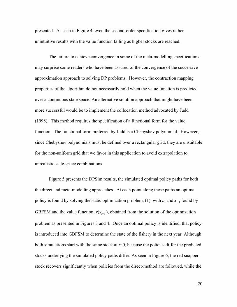
presented. As seen in Figure 4, even the second-order specification gives rather

unintuitive results with the value function falling as higher stocks are reached.

The failure to achieve convergence in some of the meta-modelling specifications

may surprise some readers who have been assured of the convergence of the successive

approximation approach to solving DP problems. However, the contraction mapping

properties of the algorithm do not necessarily hold when the value function is predicted

over a continuous state space. An alternative solution approach that might have been

more successful would be to implement the collocation method advocated by Judd

(1998). This method requires the specification of a functional form for the value

function. The functional form preferred by Judd is a Chebyshev polynomial. However,

since Chebyshev polynomials must be defined over a rectangular grid, they are unsuitable

for the non-uniform grid that we favor in this application to avoid extrapolation to

unrealistic state-space combinations.

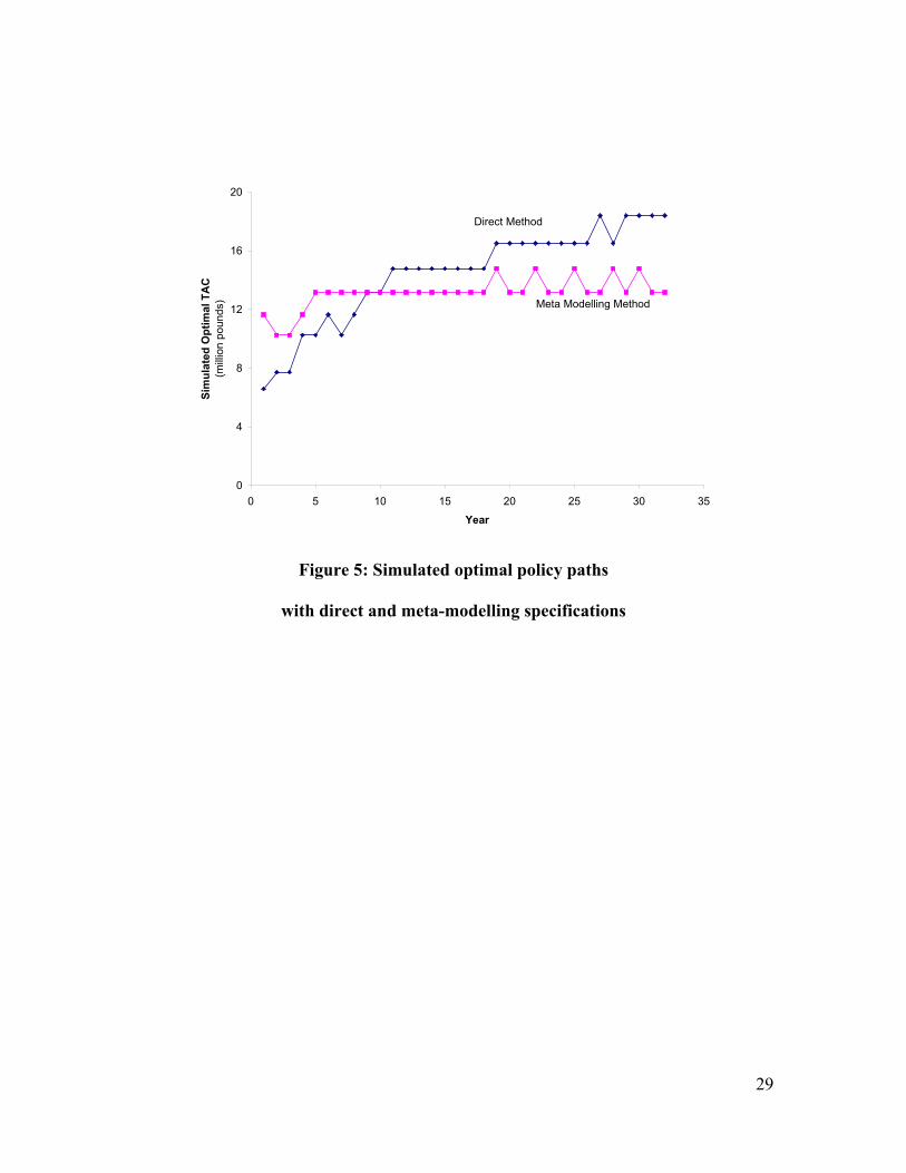
Figure 5 presents the DPSim results, the simulated optimal policy paths for both

the direct and meta-modelling approaches. At each point along these paths an optimal

policy is found by solving the static optimization problem, (1), with ut and xt+1 found by

GBFSM and the value function, v(xt+1 ), obtained from the solution of the optimization

problem as presented in Figures 3 and 4. Once an optimal policy is identified, that policy

is introduced into GBFSM to determine the state of the fishery in the next year. Although

both simulations start with the same stock at t=0, because the policies differ the predicted

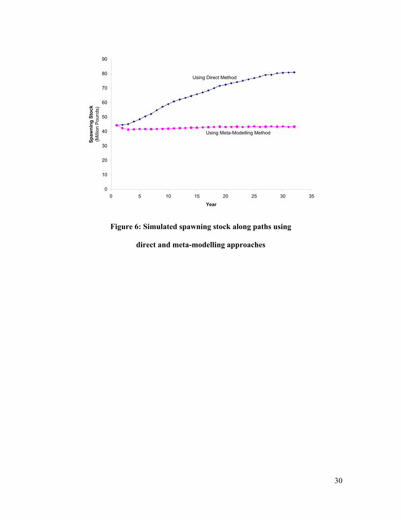
stocks underlying the simulated policy paths differ. As seen in Figure 6, the red snapper

stock recovers significantly when policies from the direct-method are followed, while the

20

stock stays essentially stable if policies from the meta-modelling approach are used.

The reason for the differences in the policies chosen must be attributable to the

value functions presented in figure 3 and 4. Because of the upward slope in the value

function identified using the direct method, there is an identified benefit to increasing the

stock. In contrast, the value function found using meta-modelling approach was not

monotonically increasing so that stock enhancements were not treated favorably when

equation (1) was evaluated to identify the optimal policies at each point in time.

The above figures give reason to believe that in this application, the direct method

is more reliable than the meta-modelling method. What is the reason for this? Recall

that either method introduces potential errors. The direct method introduces errors

through the incorrect prediction of the disaggregated stocks in period t, which then leads

to errors in the prediction of ut and xt+1. The meta method introduces errors more directly

through the inaccurate prediction of ut and xt+1. One cannot say a priori which errors will

be more important.

To compare the relative accuracy of the two methods, we compared the mean

predicted values for surplus and each of the state variables with the values that actually

were found in the simulation model along the direct method policy path in Figure 5.6 The

6 The results for the meta-method path are qualitatively similar to those from the direct-

method path, but are less interesting because of the relatively constant optimal TAC

policies used along that path.

21

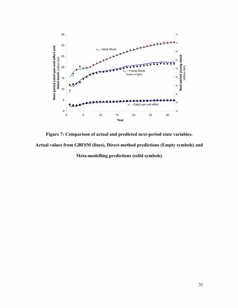
results of these comparisons are presented in Figures 7 and 8. As seen in Figure 7, either

method is reasonably precise in the prediction of the next period state variables and

neither method is preferred. Both methods err significantly in the prediction of the adult

stock in the first period few periods, but after four periods all of the predictions of the

next period’s stock were within five percent of the value simulated by GBFSM.

The results for surplus in each period, however, show important differences

between the two methods. The direct method is quite accurate in its prediction of ut,

never deviating by more than four percent from the value actually predicted by GBFSM.

This indicates either that the model is quite good at predicting the disaggregated stocks

(as is suggested by Figure 2 above) or that the distribution of the predicted returns in a

year is not very sensitive to the distribution of the cohorts, or both. In contrast, the meta-

modelling approach is quite inaccurate in its prediction of returns in a year, particularly in

the first several years when the optimal TACs are low. In the first several years, the

prediction of ut are as much as 23% below the value predicted by GBFSM. This poor

prediction of the surplus when the TAC and stocks are low, is probably an important part

of the reason that low TACs are avoided in the predicted optimal path found using the

meta-modelling approach as shown in Figure 5.

VI. Conclusions

This chapter has presented an approach to DPSim modelling, conducting dynamic

optimization with a large simulation model. Traditionally, when analysts have sought to

unify a simulation model to dynamic optimization, they have taken the meta-modelling

approach. We offer an alternative, which we call the direct method. The meta-modelling

22

approach has an important advantage in its computational burden is significantly less than

for the direct method. But we find that this benefit may have costs – in our application

the direct method provided better results. First, the value function found using the direct

method was much more plausible as it did not violate monotonicity as does the meta-

modelling approach. Secondly, the policy path seemed intuitively more reasonable, with

low TACs initially, and higher TACs once the stock has recovered. Finally, and most

importantly, we found that the direct method’s prediction of annual surplus was much

more accurate than the prediction from the meta-modelling approach.

As was found in WWG, we believe that optimal TAC management for the Gulf of

Mexico’s red snapper fishery will involve reductions in the TAC in the short term

followed by expansion in the TAC in the long-term. This policy recommendation

follows from the results of the direct method. If we instead used the meta-modelling

approach, the policy recommendation would be quite different: greater harvests in the

short term and lower harvests in the long term. The solution method makes a difference.

We wish to emphasize two important points. First, in DPSim analysis the optimal

simulation runs are carried out with the full simulation model. Regardless of the

approach taken, the DP models’ results are used only to calculate the value of future

stocks so that optimal policies at each point in time can be identified. Secondly, although

the direct method was preferred here, either approach is a plausible way to work around

the curse of dimensionality. Unless general results can be found on which of the two

methods is preferred under what conditions, we recommend that analysts use and

compare both approaches when attempting to carry out dynamic optimization linked to

23

large simulation models.

24

S1

Xt

xt

fA

Xt+1

xt+1

A

Xt+2

xt+2

A1s 1s 1s

S1 S1

ff

Figure 1: A conceptual diagram of a simulation model and the relationship with the

aggregate variables of the DP model (Reproduced with the permission of American

Agricultural Economics Association

25

0.00

0.10

0.20

0.30

0.40

0.50

0.60

0.70

0.80

0.90

1.00

0 5 10 15 20 25 30 35 40 45

Age of Cohort

R2

Depth 3

Depth 2

Figure 2: R2 values from equations used to predict

cohort populations in the direct method

26

1.8

4.1

6.4

8.8

11.1

38.248.458.668.879.089.299.4

4

4.2

4.4

4.6

4.8

5

5.2

5.4

Billions

Juvenile stock

Adult stock

Value Function

Figure 3: Value function obtained using the direct method

27

1.8

3.6

5.3

7.0

8.8

10.512.2

38.248.4

58.668.8

79.089.2

99.4

4

4.2

4.4

4.6

4.8

5

5.2

5.4

Billions

Juvenile stock

Adult stock

Value Function

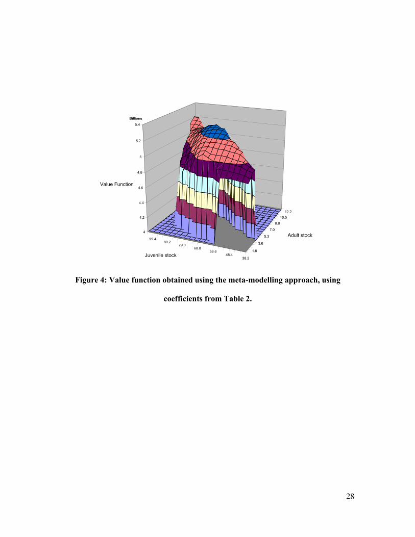
Figure 4: Value function obtained using the meta-modelling approach, using

coefficients from Table 2.

28

0

4

8

12

16

20

0 5 10 15 20 25 30 35

Year

Sim

ulat

ed O

ptim

al T

AC

(m

illio

n po

unds

) Meta Modelling Method

Direct Method

Figure 5: Simulated optimal policy paths

with direct and meta-modelling specifications

29

0

10

20

30

40

50

60

70

80

90

0 5 10 15 20 25 30 35

Year

Spaw

ning

Sto

ck

(Mill

ion

Pou

nds)

Using Meta-Modelling Method

Using Direct Method

Figure 6: Simulated spawning stock along paths using

direct and meta-modelling approaches

30

0

5

10

15

20

25

30

35

0 5 10 15 20 25 30

Year

Nex

t per

iod

catc

h-pe

r-un

it-ef

fort

and

Adu

lt st

ock

(milli

on fi

sh)

30

35

40

45

50

55

60

65

70

75

Nex

t per

iod

youn

g st

ock

(Milli

on fi

sh)

x 1 - Catch per unit effort

x 3 - Adult Stock

x 2 - Young Stock (scale on right)

Figure 7: Comparison of actual and predicted next-period state variables.

Actual values from GBFSM (lines), Direct-method predictions (Empty symbols) and

Meta-modelling predictions (solid symbols)

31

200

220

240

260

280

300

320

340

0 5 10 15 20 25 30 35

Year

Con

sum

er +

Pro

duce

r Sur

plus

(Mill

ion

Dol

lars

)

Actual SurplusPredicted - Meta MethodPredicted - Direct Method

Figure 8: Comparison of actual and predicted surplus.

Actual values from GBFSM (line), Direct-method predictions (Empty symbols)

and Meta-modelling predictions (solid symbols)

32

Equation

ut xt+1 Specification (benefits) xc xy xa

Second order polynomial 0.889 0.990 0.992 0.998 Double-log second order polynomial 0.965 0.978 0.990 0.996 Third order polynomial 0.944 0.991 0.993 0.999 Double-log third order polynomial 0.966 0.981 0.990 0.996

Table 1: R-squared values for the specifications used in the meta-modelling

approach

33

ut xt+1

(benefits) xc xy xa Intercept 17.147 -1.227 16.542 -2.260

(1.660) (0.214) (1.364) (0.456) xc 1.074 -0.499 -4.476 0.231 (1.209) (0.156) (0.993) (0.332)

xc2 -4.093 -0.102 1.898 -0.403 (0.358) (0.046) (0.294) (0.098)

xy 0.047 0.106 0.101 0.322 (0.086) (0.011) (0.070) (0.024)

xy2 0.002 -0.002 0.011 -0.004 (0.001) (0.000) (0.001) (0.000)

xa 0.047 0.203 2.578 0.233 (0.300) (0.039) (0.246) (0.082)

xa2 -0.116 0.001 0.077 -0.012 (0.017) (0.002) (0.014) (0.005)

ZT 0.320 -0.031 0.033 -0.142 (0.069) (0.009) (0.057) (0.019)

ZT2 -0.003 0.000 0.001 0.001

(0.001) (0.000) (0.001) (0.000) ZD 0.549 0.017 -0.038 -0.036

(0.101) (0.013) (0.083) (0.028) ZD

2 -0.017 0.000 0.005 0.004 (0.003) (0.000) (0.002) (0.001)

xc⋅xy 0.097 0.033 0.007 0.039 (0.030) (0.004) (0.025) (0.008)

xc⋅xa 1.457 -0.011 -0.683 0.087 (0.154) (0.020) (0.127) (0.042)

xc⋅ZT -0.079 -0.015 0.039 -0.035 (0.038) (0.005) (0.031) (0.010)

xc⋅ZD 0.289 0.006 -0.114 -0.022 (0.054) (0.007) (0.044) (0.015)

xy⋅xa -0.035 -0.001 -0.033 0.009 (0.007) (0.001) (0.006) (0.002)

xy⋅ZT 0.003 0.001 -0.003 0.002 (0.002) (0.000) (0.001) (0.000)

xy⋅ZD -0.003 0.000 0.001 -0.004 (0.003) (0.000) (0.002) (0.001)

xa⋅ZT 0.013 0.002 -0.003 0.003 (0.009) (0.001) (0.007) (0.002)

xa⋅ZD -0.028 -0.005 0.020 0.002 (0.012) (0.002) (0.010) (0.003)

ZT⋅ZD -0.016 0.001 -0.003 0.005 (0.004) (0.001) (0.003) (0.001)

R2 0.889 0.990 0.992 0.998

34

Table 2: Coefficients for second-order polynomial specification

of meta-modelling parameters

(Standard errors in parentheses)

35

VII. References

Bellman, R.E. “Functional Equations in the Theory of Dynamic Programming: Positivity

and Quasilinearity.” Proceedings of the National Academy of Sciences

41(1955):743-46.

Bertsekas, D.P. Dynamic Programming and Stochastic Control. New York: Academic

Press, 1976.

Blomo, V., K. Stokes, W. Griffin, W. Grant, and J. Nichols. “Bioeconomic Modeling of

the Gulf Shrimp Fishery: An Application to Galveston Bay and Adjacent

Offshore Areas.” Southern Journal of Agricultural Economics 10(1978):119-25.

Bryant, K.J., J.W. Mjelde, and R.D. Lacewell. "An Intraseasonal Dynamic Optimization

Model to Allocate Irrigation Water between Crops." American Journal of

Agricultural Economics 75(1993):1021-29.

Executive Office of the President. “Guidelines and Discounted Rates for Benefit-Cost

Analysis of Federal Programs.” Washington, DC: Office of Management and

Budget, 1992.

Gillig, D., W.L. Griffin, and T. Ozuna, Jr. “A Bio-Economic Assessment of Gulf of

Mexico Red Snapper Management Policies.” Transaction of the American

Fisheries Society 30(2001):117-29.

Griffin, W.L., and C. Oliver. “Evaluation of the Economic Impacts of Turtle Excluder

Devices (TEDs) on the Shrimp Production Sector in the Gulf of Mexico.” Final

Report MARFIN Award NA-87-WC-H-06139, College Station: Department of

Agricultural Economics, Texas A&M University, 1991.

36

Griffin, W.L. and J.R. Stoll. “Economic Issues Pertaining to the Gulf of Mexico Shrimp

Management Plan.” Economic Analysis for Fisheries Management Plans. L.G.

Anderson, ed., pp. 81 – 111. Ann Arbor MI: Ann Arbor Science Publishers, Inc.,

1981.

Grant, W.E., and W.L. Griffin. “A Bioeconomic Model for Gulf of Mexico Shrimp

Fishery.” Transactions of the American. Fisheries Society 108(1979):1-13.

Grant, W.E., K.G. Isaakson, and W.L. Griffin. “A General Bioeconomic Simulation

Model for Annual-Crop Marine Fisheries.” Ecological Modeling 13(1981):195-

219.

Gulf of Mexico Fishery Management Council. “Regulatory Amendment to the Reef Fish

Fishery Management Plan to Set a Red Snapper Rebuilding Plan Through 2032.”

Tampa, Florida, May 2001.

Judd, K.L. Numerical Methods in Economics. Cambridge MA: The MIT Press, 1998.

Kennedy, John O.S. Dynamic Programming: Applications to Agriculture and Natural

Resources. New York: Elsevier, 1986.

Mrkaic, M. “Policy Iteration Accelerated with Krylov Methods.” Journal of Economic

Dynamics and Control 26(2002):517-45.

Rust, J.. “Using Randomization to Break the Curse of Dimensionality.” Econometrica

65(1997a.):487-516.

Rust, J.. “Dealing with the Complexity of Economic Calculations.”

http://econwpa.wustl.edu:8089/eps/comp/papers/9610/9610002.pdf Economics

Working Paper Archive at WUSTL, Computational Economics series, 9610002,

1997b.

37

Schaller, R.R. "Moore’s Law: Past, Present, and Future." IEEE Spectrum 34(1997):53-

59.

U.S. Department of Commerce, “Fisheries of the United States; Current Fisheries

Statistics No. 2000.” National Oceanic and Atmospheric Administration, National

Marine Fisheries Service, August 2002.

van Kooten, G.C., D.L. Young, and J.A. Krautkraemer. “A Safety-First Approach to

Dynamic Cropping Decisions.” European Review of Agricultural Economics

24(1997):47-63.

Watkins, K.B., Y. Lu, and W. Huang. “Economic and Environmental Feasibility of

Variable Rate Nitrogen Fertilizer Application with Carry-Over Effects.” Journal

of Agricultural and Resource Economics 23(1998):401-26.

Woodward, R.T., Y.S. Wui and W.L. Griffin. "Living with the Curse of Dimensionality:

Closed-loop Optimization in a Large-Scale Fisheries Simulation Model"

American Journal of Agricultural Economics (Forthcoming).

38