
Electric
field
Magnetic field
X
Y
Direction of
propagation.
Z
TB5
INDIAN RAILWAYS INSTITUTE OF SIGNAL ENGINEERING & TELECOMMUNICATIONS, SECUNDERABAD - 500 017
Issued in April 2014
The Material Presented in this IRISET Notes is for guidance only. It does not over rule or alter any of the Provisions contained in Manuals or
Railway Board’s directives. IRIS
ET

TB5
RADIO PROPAGATION
CONTENTS
Chapter Description Page No
1 Radio Wave Propagation 1
2 Antenna 23
3 Annexure 39
PREPARED BY Y.V.PRASAD, ITX3
APPROVED BY C.K.PRASAD, Professor Tele
DTP AND DRAWINGS K.SRINIVAS, JE (D)
EDITION NO 02
NO. OF PAGES 50
NO.OF SHEETS 26
© IRISET
“This is the Intellectual property for exclusive use of Indian Railways. No part of this publication may be stored in a retrieval system, transmitted or reproduced in any way, including but not limited to photo copy, photograph, magnetic, optical or other record without the prior agreement and written permission of IRISET, Secunderabad, India”
www.iriset.indianrailways.gov.in
IRIS
ET

IRISET 1 TB5 – Radio Propagation
CHAPTER 1
RADIO WAVE PROPAGATION
1.0. Introduction: Radio propagation is the behavior of radio waves when they are
transmitted, or propagated from one point on the Earth to another, or into various parts of the
atmosphere. The transfer of energy through space by electromagnetic radiation at radio
frequencies.
1.1. ELECTROMAGNETIC WAVES
An electromagnetic wave consists of two fields, an electric field (E) and a magnetic field (M).
Both of these fields have a direction and a strength (or amplitude). Within the electromagnetic
wave the two fields (electric and magnetic) are oriented at precisely 90° to one another. The
fields move (by definition at the speed of light 3 x 10⁸ m/sec. or 186.000 miles/sec) in a direction
at 90° to both of them. These are transverse waves (oscillations Perpendicular to direction of
propagation). In three dimensions consider the electric field to be oriented on the y-axis, and the
magnetic field on the x-axis. Direction of travel would then be along the z-direction.
Fig. 1. The Structure of an Electromagnetic Wave
Electric and magnetic fields are actually superimposed over the top of one another but are
illustrated separately for clarity in illustration. The z-direction can be considered to be either a
representation in space or the passing of time at a single point.
As the electromagnetic wave moves the fields oscillate in direction and in strength. Figure 1
shows the electric and magnetic fields separately but they occupy the same space. They should
be over layed on one another and are only drawn this way for clarity. We could consider the z-
direction in the figure to represent passing time or it could represent a wave travelling in space at
a single instant in time.
IRIS
ET

Radio Wave Propagation
IRISET 2 TB5 – Radio Propagation
Fig. 2. Amplitude Fluctuation in an Electromagnetic Wave
Looking at the electric field from fig.1. that at the start the field is oriented from bottom to top
(increasing values of y). Sometime later the field direction has reversed. At a still later time the
field direction has reversed again and it has now reverted back to its original direction.
The curved line is intended to represent field strength. The field might start at a maximum in one
direction, decay to a zero and then build up in the other direction until it reaches a maximum in
that other direction. The field strength changes sinusoidally.
The key here is that we have two fields and they oscillate in phase. That is the electric and
magnetic fields reach their peaks and their nulls at exactly the same time and place as shown in
Fig.2. The rate of oscillation is the frequency of the wave. The distance travelled during one
period of oscillation is the wavelength. Electromagnetic waves spread uniformly in all Directions
in free space from a point Source.
Electromagnetic radiation: Power escaping into space is said to be radiated and is governed
by the characteristics of free space.
1.2. Free space: Space that does not interfere with the normal radiation and propagation of
radio waves. It does not have magnetic or gravitational Fields, solid bodies or ionized particles.
The important features of free space are:
1) Uniform everywhere
2) Contains no electrical charge
3) Carries no current
4) Infinite extent in all dimensions
Radio waves are predicted to propagate in free space by electromagnetic theory; they are a
solution to Maxwell's Equations.
E = Electric vector field represents the direction a charge will move
H = Magnetic vector field the represents directions a magnet would align
ρ = charge enclosed; J = current density; µ= permeability
ε=permittivity;
. =divergence, dot product; X=curl, vector product =Vector operator
(nabla)
IRIS
ET
Radio Wave Propagation
IRISET 3 TB5 – Radio Propagation
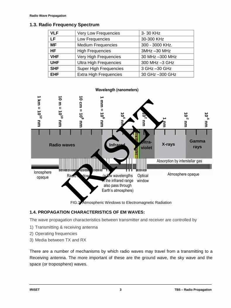
1.3. Radio Frequency Spectrum
VLF Very Low Frequencies 3- 30 KHz
LF Low Frequencies 30-300 KHz
MF Medium Frequencies 300 - 3000 KHz.
HF High Frequencies 3MHz –30 MHz
VHF Very High Frequencies 30 MHz –300 MHz
UHF Ultra High Frequencies 300 MHz –3 GHz
SHF Super High Frequencies 3 GHz –30 GHz
EHF Extra High Frequencies 30 GHz –300 GHz
FIG.3. Atmospheric Windows to Electromagnetic Radiation
1.4. PROPAGATION CHARACTERISTICS OF EM WAVES:
The wave propagation characteristics between transmitter and receiver are controlled by
1) Transmitting & receiving antenna
2) Operating frequencies
3) Media between TX and RX
There are a number of mechanisms by which radio waves may travel from a transmitting to a
Receiving antenna. The more important of these are the ground wave, the sky wave and the
space (or troposphere) waves.
10
- 4 nm
10
- 2 nm
1 n
m
10
2 nm
10
4 nm
1 m
m =
10
6 nm
10 c
m =
10
8 nm
10 m
= 1
010 n
m
1 k
m =
10
12 n
m
Radio waves Infrared Ultra-
violet X-rays
Gamma
rays
Ionosphere opaque Radio window (a few wavelengths
in the infrared range also pass through
Earth’s atmosphere)
Vis
ible
ligh
t
Optical
window
Atmosphere opaque
Absorption by interstellar gas
Wavelength (nanometers)
IRIS
ET
Radio Wave Propagation
IRISET 4 TB5 – Radio Propagation
The ground wave (also surface) wave can exist when the transmitting and receiving antennas
are close to the surface of the earth and are vertically polarized. This wave, supported at its
lower edge by the presence of the ground, is of practical importance at broadcast (i.e., medium
wave) and lower frequencies. The ground wave is vertically polarized, because any horizontal
component of the electric field in contact with earth is short-circuited by the earth. As the ground
wave passes over the surface of the earth, it is weakened as a result of energy absorbed by the
earth in the earth's resistance. The field strength of the ground wave is inversely proportional to
the square of the distance and the frequency. As a result the range for ground wave is very
limited at frequencies above 3 MHz.
The sky waves represent energy reaching the receiving antenna as a result of the reflection due
to bending of the wave path by the ionized region, termed as the ions here, which begins at
about 50 Kms above earth's surface. It accounts for practically all-very long distance HP radio
communication. Frequencies above 30 MHz are not capable of being reflected back by the
ionosphere even at low angles of take off and as such this method of communication is of
importance for frequencies below 30 MHz
Line of Sight Propagation (LOS) The simplest form of propagation is line of site. All
frequencies will function in this form. Distance between the transmitter and receiver is dependent
on the frequency / wavelength of the signal. Line of site propagation is very useful at VHF and
UHF Frequencies.
1.4.1 Ground-wave propagation: Ground wave propagation is particularly important on the
LF and MF portion of the radio spectrum. Ground wave radio propagation is used to provide
relatively local radio communications coverage, especially by radio broadcast stations that
require to cover a particular locality. Ground wave radio signal propagation is ideal for relatively
short distance propagation on these frequencies during the daytime. Sky-wave ionospheric
propagation is not possible during the day because of the attenuation of the signals on these
frequencies caused by the D region in the ionosphere. In view of this, radio communications
stations need to rely on the ground-wave propagation to achieve their coverage.
A ground wave radio signal is made up from a number of constituents. If the antennas are in the
line of sight then there will be a direct wave as well as a reflected signal. As the names suggest
the direct signal is one that travels directly between the two antenna and is not affected by the
locality. There will also be a reflected signal as the transmission will be reflected by a number of
objects including the earth's surface and any hills, or large buildings. That may be present.
In addition to this there is surface wave. This tends to follow the curvature of the Earth and
enables coverage to be achieved beyond the horizon. It is the sum of all these components that
is known as the ground wave.
Beyond the horizon the direct and reflected waves are blocked by the curvature of the Earth, and
the signal is purely made up from the diffracted surface wave. It is for this reason that surface
wave is commonly called ground wave propagation.
IRIS
ET

Radio Wave Propagation
IRISET 5 TB5 – Radio Propagation
1.4.1.1 Effect of frequency on ground wave propagation: As the wave front of the ground wave travels along the Earth's surface it is attenuated. The
degree of attenuation is dependent upon a variety of factors. Frequency of the radio signal is
one of the major determining factor as losses rise with increasing frequency. As a result it makes
this form of propagation impracticable above the bottom end of the HF portion of the spectrum (3
MHz). Typically a signal at 3.0 MHz will suffer an attenuation that may be in the region of 20 to
60 dB more than one at 0.5 MHz dependent upon a variety of factors in the signal path including
the distance. In view of this it can be seen why even high power HF radio broadcast stations
may only be audible for a few miles from the transmitting site via the ground wave.
FIG.4.ground wave
Ground Wave = Direct Wave + Reflected Wave + Surface Wave. At MF and in the lower HF
bands, aerials tend to be close to the ground (in terms of wavelength). Hence the direct wave
and reflected wave tend to cancel each other out (there is a 180 degree phase shift on
reflection). This means that only the surface wave remains. A surface wave travels along the
surface of the earth by virtue of inducing currents in the earth. The imperfectly conducting earth
leads to some of its characteristics. Its range depends upon: Frequency, Polarization, Location
and Ground Conductivity. The surface waves dies more quickly as the frequency increases;
1.4.2. Sky waves or Ionospheric waves:
It is the upper portion of the atmosphere (between approx.50km and 400km above the Earth). In
this region, gases get ionized by absorbing large quantities of radiation and form different layers.
Ionization increases with altitude. Variation is not linear, but tends to be the amount of ionization
depends upon the rate of formation of the ions and the rate of recombination. At lower altitudes
since the atmospheric pressure is large the rate of combination is large so that ionization is
small. At higher altitudes since the atmospheric pressure is low the rate of re-combination is
small so that ionization so that ionization is large.
1.4.2.1. Ionospheric propagation:
Here the radio signals are modified and influenced by the action of the free electrons in the
upper reaches of the earth's atmosphere called the ionosphere. This form of radio propagation is
used by stations on the short wave bands for their signals to be heard around the globe.
IRIS
ET

Radio Wave Propagation
IRISET 6 TB5 – Radio Propagation
As electromagnetic waves, and in this case, radio signals travel, they interact with objects and
the media in which they travel. As they do this the radio signals can be reflected, refracted or
diffracted. These interactions cause the radio signals to change direction, and to reach areas
which would not be possible if the radio signals travelled in a direct line.
HF radio communications is dependent for most of its applications on the use of the ionosphere.
This region in the atmosphere enables radio communications signals to be reflected, or more
correctly refracted back to earth so that they can travel over great distances around the globe.
Ionospheric propagation is normally as an HF propagation mode, although, it use can extend
above and below the HF portion of the spectrum on many occasions.
The fact that radio communications signals can travel all over the globe on the HF bands is
widely used by many by broadcasters, news agencies, maritime, radio hams and many other
users. Radio transmitters using relatively low powers can be used to communicate to the other
side of the globe. Although radio propagation using the ionosphere may not be not as reliable as
that provided by satellites, it nevertheless provides a very cost effective and efficient form of
radio communication. To enable the most to be made of ionospheric propagation many radio
users make extensive use of HF propagation programmes to predict the areas of the globe to
which signals may travel, or the probability of them reaching a given area.
Radio communications signals in the medium and short wave bands travel by two basic means.
The first is known as a ground wave (covered on a separate page in this section), and the
second a sky wave using the ionosphere.
Indirect or Obstructed Propagation
The efficacy of indirect propagation depends upon the amount of margin in the communication
link and the strength of the diffracted or reflected signals. The operating frequency has a
significant impact on the viability of indirect propagation, with lower frequencies working the best.
1.5. Ionosphere Regions The part of the ionosphere that is primarily responsible for “sky-
wave” exists in 3 to 4 layers depending on the time of day. These layers exist at differing
altitudes.
FIG. 5 . Regions of space
D= layer-1
E = layer-2
F1 = layer-3
F2= layer-4
IRIS
ET

Radio Wave Propagation
IRISET 7 TB5 – Radio Propagation
1.5.1. Description of the layers in the Ionosphere:
D layer: The D layer is the lowest of the layers of the ionosphere. It exists at altitudes around
60 to 90 km. It is present during the day when radiation is received from the sun. However the
density of the air at this altitude means that ions and electrons recombine relatively quickly. This
means that after sunset, electron levels fall and the layer effectively disappears. This layer is
typically produced as the result of X-ray and cosmic ray ionization. It is found that this layer
tends to attenuate signals that pass through it.
E layer: The next layer beyond the D layer is called the E layer. This exists at an altitude of
between 100 and 125 km. Instead of acting chiefly as an attenuator, this layer reflects radio
signals although they still undergo some attenuation.
In view of its altitude and the density of the air, electrons and positive ions recombine relatively
quickly. This occurs at a rate of about four times that of the F layers that are higher up where the
air is less dense. This means that after nightfall the layer virtually disappears although there is
still some residual ionization.
F layer: The F layer is the most important region for long distance HF communications. During
the day it splits into two separate layers. These are called the F1 and F2 layers, the F1 layer
being the lower of the two. At night these two layers merge to give one layer called the F layer.
The altitudes of the layers vary considerably with the time of day, season and the state of the
sun. Typically in summer the F1 layer may be around 300 km with the F2 layer at about 400 km
or even higher. In winter these figures may be reduced to about 300 km and 200 km. Then at
night the F layer is generally around 250 to 300 km. Like the D and E layers, the level of
ionization falls at night, but in view of the much lower air density, the ions and electrons combine
much more slowly and the F layer decays much less. Accordingly it is able to support radio
communications, although changes are experienced because of the lessening of the ionization
levels. The ionization of all the layers is maximum at day time and minimum at night.
1.6. Tropospheric Propagation Consists the reflection or refraction of the RF waves from temperature and moisture layers in the
atmosphere. Here the signals are influenced by the variations of refractive index in the
troposphere just above the earth's surface. Tropospheric radio propagation is often the means
by which signals at VHF and above are heard over extended distances. On frequencies above
30 MHz, it is found that the troposphere has an increasing effect on radio signals and radio
communications systems. The radio signals are able to travel over greater distances than would
be suggested by line of sight calculations. At times conditions change and radio signals may be
detected over distances of 500 or even 1000 km and more. This is normally by a form of
tropospheric enhancement, often called "tropo" for short. At times signals may even be trapped
in an elevated duct in a form of radio signal propagation known as tropospheric ducting. This can
IRIS
ET

Radio Wave Propagation
IRISET 8 TB5 – Radio Propagation
disrupt many radio communications links (including two way radio communications links)
because interference may be encountered that is not normally there. As a result when designing
a radio communications link or network, this form of interference must be recognized so that
steps can be taken to minimize its effects.
The way in which signals travel at frequencies of VHF and above is of great importance for those
looking at radio coverage of systems such as cellular telecommunications, mobile radio
communications and other wireless systems as well as other users including radio hams.
1.7. Propagation in the HF Bands:
Without ionization of the atmosphere due to the sun‘s energy, HF propagation would be limited
to line of site.
1.8. Propagation on the VHF Bands
VHF propagation is principally line of site but much longer paths are possible with Ionization of
the atmosphere‘s E-layer phenomena. Due to re-entry of meteors will also create a condition for
VHF long distance propagation. One new method of long distance VHF communication results
from bouncing VHF signals off high altitude commercial airliners.
1.9. Propagation on the UHF Bands
UHF propagation is basically line of site. Some long range propagation is possible with E-Layer
phenomena. UHF is used mainly for local communication. Sometimes UHF can be part of a wide
area repeater system allowing for interstate communication.
1.10. Radio Wave Behavior
Radio waves, like light waves, exhibit certain characteristics when coming into contact with
objects. Here are some of the possible behaviors.
1.10.1. Reflection: Reflection occurs when a radio wave hits an object that has a dimension is
larger than the wavelength of the radio wave. The radio wave is then reflected off the surface.
Fig.6. Reflection of a radio wave
Reflection occurs when signal encounters a surface that is large relative to the wavelength of the
signal · Radio waves may be reflected from various substances or objects they meet during
travel between the transmitting and receiving sites. The amount of reflection depends on the
reflecting material. Smooth metal surfaces of good electrical conductivity are efficient reflectors
of radio waves. The surface of the Earth itself is a fairly good reflector. The radio wave is not
reflected from a single point on the reflector but rather from an area on its surface. The size of
the area required for reflection to take place depends on the wavelength of the radio wave and
IRIS
ET

Radio Wave Propagation
IRISET 9 TB5 – Radio Propagation
the angle at which the wave strikes the reflecting substance. When radio waves are reflected
from flat surfaces, a phase shift in the alternations of the wave occurs· The shifting in the phase
relationships of reflected radio waves is one of the major reasons for fading.
1.10.2. Refraction
Refraction occurs when a radio wave hits an object of a higher density than its current medium.
The radio wave now travels at a different angle. An example would be radio waves propagating
through clouds. The bending, or change of direction, is always toward the medium that has the
lower velocity of propagation.
Fig.7.Refraction of a radio wave
1.10.3. Scattering
Scattering occurs when a radio wave hits an object of irregular shape, usually an object with a
rough surface area and the radio wave bounces off in multiple directions.
Fig.8.Scattering of a radio wave
1.10.4. Absorption
Absorption occurs when a radio wave hits an object that does not cause it to be reflected,
refracted, or scattered, so it is absorbed by the object. The radio wave is then lost.
Fig.9. Absorption of a radio wave
Radio waves are subject to interference caused by objects and obstacles in the air. Such
obstacles can be concrete walls, metal cabinets, or even raindrops. In general, transmissions
made at higher frequencies are more subject to radio absorption (by the obstacles) and larger
signal loss. Larger frequencies have smaller wavelengths, and hence signals with smaller
wavelengths tend to be absorbed by the obstacles that they collide with. This causes high
frequency devices to have a shorter operating range.
For devices that transmit data at high frequencies, much more power is needed in order for them
to cover the same range as compared to lower frequency transmitting devices.
IRIS
ET

Radio Wave Propagation
IRISET 10 TB5 – Radio Propagation
1.10.5. Diffraction
Diffraction is a phenomenon that takes place when the radio wave strikes a surface and changes
its direction of propagation owing to the inability of the surface to absorb it. The loss due to
diffraction depends upon the kind of obstruction in the path.
Sometimes a radio wave will be blocked by objects standing in its path. In this case, the radio
wave is broken up and bends around the corners of the object. It is this property that allows
radio waves to operate without a visual line of sight.
Fig. 10. Diffraction of radio waves
Diffraction is the name given to the mechanism by which waves enter into the shadow of an
obstacle. Diffraction occurs at the edge of an impenetrable body that is large compared to
wavelength of radio wave. A radio wave that meets an obstacle has a natural tendency to bend
around the obstacle. The bending, called diffraction, results in a change of direction of part of the
wave energy from the normal line-of-sight path. This change makes it possible to receive energy
around the edges of an obstacle.
The ratio of the signal strengths without and with the obstacle is referred to as the diffraction
loss. The diffraction loss is affected by the path geometry and the frequency of operation. The
signal strength will fall by 6 dB as the receiver approaches the shadow boundary, but before it
enters into the shadow region. Deep in the shadow of an obstacle, the diffraction loss increases
with 10*log (frequency). So, if double the frequency, deep in the shadow of an obstacle the loss
will increase by 3 dB. This establishes a general truth, namely that radio waves of longer
wavelength will penetrate more deeply into the shadow of an obstacle.
In practice, the mobile antenna is at a much lower height than the base station antenna, and
there may be high buildings or hills in the area. Thus, the signal undergoes diffraction in
reaching the mobile antenna. This phenomenon is also known as ‗shadowing‘ because the
mobile receiver is in the shadow of these structures.
1.10.6.Building and Vehicle Penetration
When the signal strikes the surface of a building, it may be diffracted or absorbed. If it is to some
extent absorbed the signal strength is reduced. The amount of absorption is dependent on the
type of building and its environment: the amount of solid structure and glass on the outside
IRIS
ET

Radio Wave Propagation
IRISET 11 TB5 – Radio Propagation
surface, the propagation characteristics near the building, orientation of the building with respect
to the antenna orientation, etc. This is an important consideration in the coverage planning of a
radio network.
Vehicle penetration loss is similar, except that the object in this case is a vehicle rather than a
building.
Fig.11.Factors affecting wave propagation: (1) direct signal; (2) diffraction; (3) vehicle penetration; (4) interference; (5) building penetration
1.11. Fresnel Zone
Radio waves diffracted by objects can affect the strength of the received signal. This happens
even though the obstacle does not directly obscure the direct visual path. This area, known as
the "Fresnel Zone", and must be kept clear of all obstructions
Fig.12.Fresnel zone
Where d1 and d2 = km, f = GHz, h = meters.
IRIS
ET

Radio Wave Propagation
IRISET 12 TB5 – Radio Propagation
The 1st Fresnel zone is a spheroid space formed within the trajectory of the path when the path
difference when radio wave energy reaches the receiver by the shortest distance, and when it
gets there by another route, is within λ/2. Odd-numbered Fresnel zones have relatively intense
field strengths, whereas even numbered Fresnel zones are nulls. When the radio signal pass
from site A to site B, the lack of adequate Fresnel Zone clearance caused signal diffraction, and
degradation of the radio signal. If the 1st Fresnel zone is not clear, then free-space loss does not
apply and an adjustment term must be included.
To avoid this have to use an antenna with a narrower lobe pattern, usually a higher gain antenna
will achieve this.Raise the antenna mounting point on Site A and/or Site B.
1.12 Multipath
Multipath is a term used to describe the multiple paths a radio wave may follow between
transmitter and receiver. Such propagation paths include the ground wave, ionospheric
refraction, and reradiation by the ionospheric layers, reflection from the Earth's surface or from
more than one ionospheric layer, etc. If the two signals reach the receiver in-phase (both signals
are at the same point in the wave cycle when they reach the receiver), then the signal is
amplified. This is known as an ―up fade.‖ If the two waves reach the receiver out-of-phase (the
two signals are at opposite points in the wave cycle when they reach the receiver), they weaken
the overall received signal. If the two waves are 180º apart when they reach the receiver, they
can completely cancel each other out so that a radio does not receive a signal at all. A location
where a signal is canceled out by multipath is called a ―null‖ or ―down fade.‖
1.13. Fading
As the signal travels from the transmitting antenna to the receiving antenna, it loses strength.
This may be due to the phenomenon of path loss or it may be due to the Rayleigh effect.
Rayleigh fading is due to the fast variation of the signal level both in terms of amplitude and
phase between the transmitting and receiving antennas when there is no line-of-sight. Rayleigh
fading can be divided into two kinds: multipath fading and frequency-selective fading.
Reduction in received signal strength due to fluctuations in radio path caused by non-
homogenous and time varying atmospheric parameters is called Fading. Arrival of the same
signal from different paths at different times and its combination at the receiver causes the signal
to fade. This phenomenon is multipath fading and is a direct result of multipath propagation.
Multipath fading can cause fast fluctuations in the signal level. This kind of fading is independent
of the downlink or uplink if the bandwidths used are different from each other in both directions.
Frequency-selective fading takes place owing to variation in atmospheric conditions.
Atmospheric conditions may cause the signal of a particular frequency to fade. When the mobile
station moves from one location to another, the phase relationship between the various
components arriving at the mobile antenna changes, thus changing the resultant signal level.
Doppler shift in frequency takes place owing to the movement of the mobile with respect to the
receiving frequencies.
IRIS
ET

Radio Wave Propagation
IRISET 13 TB5 – Radio Propagation
1.13.1. Types of Fading
1.13.1.1. Fast fading - occurs when the coherence time of the channel is small relative to the
delay constraint of the channel. Fast fading causes rapid fluctuations in phase and amplitude of
a signal if a transmitter or receiver is moving or there are changes in the radio environment (e.g.
car passing by). If a transmitter or receiver is moving, the fluctuations occur within a few wave
lengths. Because of its short distance fast fading is considered as small-scale fading.
Coherence time: For an electromagnetic wave, the time over which a propagating wave may be
considered coherent. In long-distance transmission systems, the coherence time may be
reduced by propagation factors such as dispersion, scattering, and diffraction.
1.13.1.2. Slow fading - arises when the coherence time of the channel is large relative to the
delay constraint of the channel. Slow fading occurs due to the geometry of the path profile. This
leads to the situation in which the signal gradually gets weaker or stronger.
1.13.1.3. Flat fading – Occurs when the coherence bandwidth of the channel is larger than the
bandwidth of the signal. The coherence bandwidth of a wireless channel is the range of
frequencies that are allowed to pass through the channel without distortion.
Coherence bandwidth is a statistical measurement of the range of frequencies over which the
channel can be considered "flat", or in other words the approximate maximum bandwidth or
frequency interval over which two frequencies of a signal are likely to experience comparable or
correlated amplitude fading. If the multipath time delay spread equals D seconds, then the
coherence bandwidth in rad/s is given approximately by the equation:
Also coherence bandwidth in Hz is given approximately by the equation:
It can be reasonably assumed that the channel is flat if the coherence bandwidth is greater than
the data signal bandwidth. The coherence bandwidth varies over cellular or PCS
communications paths because the multipath spread D varies from path to path.
Frequencies within a coherence bandwidth of one another tend to all fade in a similar or
correlated fashion. One reason for designing the spread spectrum (CDMA IS-95) waveform with
a bandwidth of approximately 1.25 MHz is because in many urban signaling environments the
coherence bandwidth Wc is significantly less than 1.25 MHz. Therefore, when fading occurs it
occurs only over a relatively small fraction of the total CDMA signal bandwidth. The portion of
the signal bandwidth over which fading does not occur typically contains enough signal power to
sustain reliable communications. This is the bandwidth over which the channel transfer function
remains virtually constant.
IRIS
ET

Radio Wave Propagation
IRISET 14 TB5 – Radio Propagation
Fig. 13. Flat fading
Flat Fading is caused by absorbers between the two antennae and is countered by antenna
placement and transmit power level.
1.13.1.4. Selective fading – occurs when the coherence bandwidth of the channel is smaller
than the bandwidth of the signal.
Fig. 14.Selective fading
Frequency selective fading is caused by reflectors between the transmitter and receiver creating
multi-path effects.
Effects of Frequency Selective Fading 1. The dips or fades in the response due to reflection cause cancellation of certain frequencies
at the Receiver.
2. Reflections off near-by objects (e.g. ground, buildings, trees, etc) can lead to multi-path
signals of similar signal power to the direct signal.
3. This can result in deep nulls in the received signal power due to destructive interference.
IRIS
ET

Radio Wave Propagation
IRISET 15 TB5 – Radio Propagation
1.13.1.5. Rayleigh fading – Rayleigh fading is the name given to the form of fading that is often
experienced in an environment where there is a large number of reflections present. The
Rayleigh fading model uses a statistical approach to analyse the propagation, and can be used
in a number of environments.
The Rayleigh fading model is normally viewed as a suitable approach to take when analysing
radio wave propagation performance for areas such as cellular communications in a well built up
urban environment where there are many reflections from buildings, etc.. HF ionospheric radio
wave propagation where reflections (or more exactly refractions) occur at many points within the
ionosphere is also another area where Rayleigh fading model applies. It is also appropriate to
use the Rayleigh fading model for tropospheric radio propagation because, again there are
many reflection points and the signal may follow a variety of different paths. Assume that the
magnitude of a signal that has passed through a communications channel will vary randomly.
Fig.15. Rayleigh fading
1.13.1.6. Multipath (Nakagami) fading - occurs for multipath scattering with relatively larger
time delay spreads, with different clusters of reflected waves.
Fig.16. Multi-path fading
When the waves of multi-path signals are out of phase, reduction of the signal strength at the
receiver can occur. Multi-path can also cause inter-symbol interference.
IRIS
ET

Radio Wave Propagation
IRISET 16 TB5 – Radio Propagation
1.13.2. Fade Margin
Fade margin is the difference between the unfaded receive signal level and the receiver
sensitivity threshold. Each link must have sufficient fade margin to protect against path fading
that weakens the radio signals.
A design allowance in radio link budget, that provides sufficient system gain or sensitivity to
accommodate expected fading, for the purpose of ensuring that the required quality of service is
maintained. The amount by which a received signal level may be reduced without causing
system performance to fall below a specified threshold value.
Number of decibels of attenuation which may be added to a specified radio-frequency
propagation path before the signal-to-noise ratio of a specified channel falls below a specified
minimum in order to avoid fading.
Network engineers need to know link performance factors to design wireless networks that meet
performance expectations in the given environment. Link budget calculations are used to
determine the placement of network elements. Link budget is the difference between transmit
power and receiver sensitivity and indicates the amount of attenuation while still supporting
communication. Fade margin is a design cushion allowance for fluctuations of the received
signal‘s strength. These fluctuations are caused by:
1. Interference in the operating band
2. Movement of the transmitter or the receiver
3. Reflections or scattering due to the objects in the vicinity 1.13.2.1. Factors that affect the Link Budget
Path loss is the energy that is lost between the transmitter and the receiver. Many factors can
cause signals to lose energy. Network architects need to understand transmission losses
attributed to:
a. Obstructions such as trees or buildings
b. Reflections from buildings or bodies of water
c. Insufficient antenna height
d. Environmental conditions such as humidity, precipitation or ice
Adequate allowance for fading is essential to ensure that an RF link is available at all times.
Allowing for more fade margin will increase link reliability, but will also reduce the distance
between modules
IRIS
ET

Radio Wave Propagation
IRISET 17 TB5 – Radio Propagation
1.13.2.1. Radio Link
Fig. 17.Radio link
The formulas below can be used to calculate if the radio link has an acceptable fade margin or, if
not, how much antenna gain that needs to be added or if repeaters have to be used.
The known factors are often:
1. The distance between two sites
2. The (possible) height of the antennas
3. The transmit power of the radio
4. The receiver sensitivity of the radio
5. The antenna gain This is a calculation with all the possible losses in the system and subtracting the losses from
the line of sight to give an estimated value of your likely link performance
FM = Srx + Ptx + Gtx + FSL + Grx – CL
FM = Fade Margin
Srx = Sensitivity of the receiver (dBm) (using +dBm instead of –dBm)
Ptx = Transmitter RF output power (dBm)
Gtx = TX Antenna Gain (dB)
FSL = Free Space Loss (dB) = 32.4 + 20 Log f + 20 log d
Grx = Receiver (RX) Antenna Gain (dB)
CL = Cable/Connector Loss (dB)
IRIS
ET

Radio Wave Propagation
IRISET 18 TB5 – Radio Propagation
Calculation of fade margin FM (A typical example):
Distance = 5 kilometers
Antenna height 1 = 20 meters
Antenna height 2 = 5 meters
Radio Tx Power = 33 dBm (2 W)
Radio Rx Sensitivity = -110 dBm
Frequency = 456.000 MHz
Antenna Gain 1 = 3 dBd
Antenna Gain 2 = 6 dBd
Cable / Connector losses = 4 dB total
FM = ?
FSL = 129 dB (frequency & distance dependant value)
FSL = 32.44+ 20 log F + 20 Log D
Where F is in MHz and D is in Kms
FM = Srx + Ptx + Gtx - FSL+ Grx – Cl
FM = 110 dBm + 33 dBm + 3 dBd – 129 dB + 6 dBd – 4 dB = 19 dB The fade margin is 19 dB, which is an acceptable level. The radio link should be possible. 1.14. Diversity Techniques
Diversity: It is the technique used to compensate for fading channel impairments. It is
implemented by using two or more receiving antennas. Diversity is usually employed to reduce
the depth and duration of the fades experienced by a receiver in a flat fading channel.
Fade margin on the transmitter path is not an efficient solution at all, and one alternate solution
is to take the advantage of the statistical behavior of the fading channel. This is the basic
concept of Diversity, where two or more inputs at the receiver are used to get uncorrelated
signals.
1.14.1. Frequency Diversity: The same information signal is transmitted and received
simultaneously on two or more independent fading carrier frequencies. Different frequencies
mean different wavelengths. The hop when using frequency diversity (Separation of carriers) is
that the same physical multipath routes will not produce simultaneous deep fades at two
separate wavelengths.
Fig.18. Frequency Diversity
IRIS
ET

Radio Wave Propagation
IRISET 19 TB5 – Radio Propagation
Fig.19.Block diagram of Frequency Diversity
ADVANTAGES
1. Reliability is more
2. Equivalent to 100% hot standby, hence no need of providing stand by TX or RX.
DISADVANTAGES
1. Two frequencies are needed
2. Improvement by diversity is not much, since 5% separation of frequency is rarely achieved. 1.14.2. Space Diversity
A method of transmission or reception, or both, in which the effects of fading are minimized by
the simultaneous use of two or more physically separated antennas, ideally separated by one
half or more wavelengths. Deep multipath fade have unlucky occurrence when the receiving
antenna is in exactly in the ‗wrong‘ place. One method of reducing the likelihood of multipath
fading is by using two receive antennas (Separation of antennas) and using a switch to select
the better signal. If these are physically separated then the probability of a deep fade occurring
simultaneously at both of these antennas is significantly reduced.
Fig.20. Space Diversity
IRIS
ET

Radio Wave Propagation
IRISET 20 TB5 – Radio Propagation
Fig.21.Block diagram of space Diversity
ADVANTAGES 1. One frequency is used.
2. Propagation reliability is improved.
3. For more vertical separation of antennas, improvement factor can be more. DISADVANTAGES 1. The two antennas are kept on the same tower. The lower antenna should be in Line of Sight
with the TX antenna. Hence length of tower may increase beyond 100m.
2. Costly
3. Good tower foundation necessary, since wind pressure will be large.
4. Equipment reliability decreased, hence stand by required 1.14.3. Angle Diversity Angle diversity reception in which several antennas are used pointing in different directions with
generally a small angular separation. In this case the receiving antennas are co-located but have
different principal directions.
1.14.4. Polarization Diversity This involves simultaneously transmitting and receiving on two orthogonal polarizations (e.g.
horizontal and vertical). The hope is that one polarization will be less severely affected when the
other experiences a deep fade.
1.14.5. Time Diversity This will transmit the desired signal in different periods of time. The intervals between
transmissions of the same symbol should be at least the coherence time so that different copies
of the same symbol undergo independent fading.
IRIS
ET

Radio Wave Propagation
IRISET 21 TB5 – Radio Propagation
1.15. Effects of Rain, Snow and Fog The loss of LOS paths may sometimes be affected by weather conditions. Rain and fog (clouds)
become a significant source of attenuation only when we get well into the microwave region.
Attenuation from fog only becomes noticeable (i.e., attenuation of the order of 1 dB or more)
above about 30 GHz. Snow is in this category as well. Rain attenuation becomes significant at
around 10 GHz, where a heavy rainfall may cause additional path loss of the order of 1 dB/km.
Propagation of a Signal over Water Propagation over water is a big concern for radio planners. The reason is that the radio signal
might create interference with the frequencies of other cells. Moreover, as the water surface is a
very good reflector of radio waves, there is a possibility of the signal causing interference to the
antenna radiation patterns of other cells.
1.15.1. Essential Features of Rain Scatter the received signal strength is proportional to 1. transmitted power (obviously)
2. the common volume (this is the antenna beam intersection),
3. the particle density (for example how hard it is raining)
4. the scattering function So2 (how well the particles scatter And inversely proportional to: 1. the 4th power of range
2. the 4th power of the wavelength Of course, the rain also attenuates the energy in the radio wave, so the scattered power at the
receiver will be reduced.
1.16. Propagation of a Signal over Vegetation (Foliage Loss) Foliage loss is caused by propagation of the radio signal over vegetation, principally forests. The
variation in signal strength depends upon many factors, such as the type of trees, trunks, leaves,
branches, their densities, and their heights relative to the antenna heights. Foliage loss depends
on the signal frequency and varies according to the season.
Trees can be a significant source of path loss, and there are a number of variables involved,
such as the specific type of tree, whether it is wet or dry, and in the case of deciduous trees,
whether the leaves are present or not. Isolated trees are not usually a major problem, but a
dense forest is another story.
The attenuation depends on the distance the signal must penetrate through the forest, and it
increases with frequency. According to a CCIR report, the attenuation is of the order of 0.05
dB/m at 200 MHz, 0.1 dB/m at 500 MHz, 0.2 dB/m at 1 GHz, 0.3 dB/m at 2 GHz and 0.4 dB/m at
3 GHz.
IRIS
ET

Radio Wave Propagation
IRISET 22 TB5 – Radio Propagation
At lower frequencies, the attenuation is somewhat lower for horizontal polarization than for
vertical, but the difference disappears above about 1 GHz. This adds up to a lot of excess path
loss if your signal must penetrate several hundred meters of forest! Fortunately, there is also
significant propagation by diffraction over the treetops, especially if you can get your antennas
up near treetop level or keep them a good distance from the edge of the forest, so all is not lost if
you live near a forest.
IRIS
ET

Antenna
IRISET 23 TB5 – Radio Propagation
CHAPTER 2
ANTENNA
2.0. Introduction
By definition, an antenna is a device used to transform an RF signal, traveling on a conductor,
into an electromagnetic wave in free space. Antennas demonstrate a property known as
reciprocity, which means that an antenna will maintain the same characteristics regardless if it is
transmitting or receiving. Most antennas are resonant devices, which operate efficiently over a
relatively narrow frequency band. An antenna must be tuned to the same frequency band of the
radio system to which it is connected; otherwise the reception and the transmission will be
impaired. When a signal is fed into an antenna, the antenna will emit radiation distributed in
space in a certain way. A graphical representation of the relative distribution of the radiated
power in space is called a radiation pattern.
2.1. Antenna Glossary: A few common terms that related to antenna are defined and explained
below:
2.1.1. Input Impedance
For an efficient transfer of energy, the impedance of the radio, of the antenna and of the
transmission cable connecting them must be the same. Transceivers and their transmission
lines are typically designed for 50Ω impedance. If the antenna has impedance different from
50Ω, then there is a mismatch and an impedance matching circuit is required.
2.1.2. Return loss
The return loss is another way of expressing mismatch. It is a logarithmic ratio measured in dB
that compares the power reflected by the antenna to the power that is fed into the antenna from
the transmission line. The relationship between SWR and return loss is the following:
Return Loss (in dB) = 20 log10 SWR SWR -1
2.1.3. Bandwidth The bandwidth of an antenna refers to the range of frequencies over which the antenna can
operate correctly. The antenna's bandwidth is the number of Hz for which the antenna will
exhibit an SWR less than 2:1. The bandwidth can also be described in terms of percentage of
the center frequency of the band.
BW = 100 × FH ----- FL
FC
Where FH is the highest frequency in the band, FL is the lowest frequency in the band, and FC is
the center frequency in the band. In this way, bandwidth is constant relative to frequency. If
bandwidth was expressed in absolute units of frequency, it would be different depending upon
the center frequency. Different types of antennas have different bandwidth limitations.
IRIS
ET

Antenna
IRISET 24 TB5 – Radio Propagation
2.1.4. Directivity and Gain
Directivity is the ability of an antenna to focus energy in a particular direction when transmitting,
or to receive energy better from a particular direction when receiving. In a static situation, it is
possible to use the antenna directivity to concentrate the radiation beam in the wanted direction.
However in a dynamic system where the transceiver is not fixed, the antenna should radiate
equally in all directions, and this is known as an omni-directional antenna.
Gain is not a quantity which can be defined in terms of a physical quantity such as the Watt or
the Ohm, but it is a dimensionless ratio. Gain is given in reference to a standard antenna. The
two most common reference antennas are the isotropic antenna and the resonant half-wave
dipole antenna. The isotropic antenna radiates equally well in all directions. Real isotropic
antennas do not exist, but they provide useful and simple theoretical antenna patterns with
which to compare real antennas. Any real antenna will radiate more energy in some directions
than in others. Since it cannot create energy, the total power radiated is the same as an isotropic
antenna, so in other directions it must radiate less energy.
The gain of an antenna in a given direction is the amount of energy radiated in that direction
compared to the energy an isotropic antenna would radiate in the same direction when driven
with the same input power. Usually we are only interested in the maximum gain, which is the
gain in the direction in which the antenna is radiating most of the power. An antenna gain of 3 dB
compared to an isotropic antenna would be written as 3 dBi. The resonant half-wave dipole can
be a useful standard for comparing to other antennas at one frequency or over a very narrow
band of frequencies. To compare the dipole to an antenna over a range of frequencies requires
a number of dipoles of different lengths. An antenna gain of 3 dB compared to a dipole antenna
would be written as 3 dBd.
The method of measuring gain by comparing the antenna under test against a known standard
antenna, which has a calibrated gain, is technically known as a gain transfer technique. Another
method for measuring gain is the 3 antennas method, where the transmitted and received power
at the antenna terminals is measured between three arbitrary antennas at a known fixed
distance.
2.1.5. Radiation Pattern
The radiation or antenna pattern describes the relative strength of the radiated field in various
directions from the antenna, at a constant distance. The radiation pattern is a reception pattern
as well, since it also describes the receiving properties of the antenna. The radiation pattern is
three-dimensional, but usually the measured radiation patterns are a two dimensional slice of the
three-dimensional pattern, in the horizontal or vertical planes. These pattern measurements are
presented in either a rectangular or a polar format. The following figure shows a rectangular plot
presentation of a typical 10 element Yagi. The detail is good but it is difficult to visualize the
antenna behavior at different directions.
IRIS
ET
Antenna
IRISET 25 TB5 – Radio Propagation
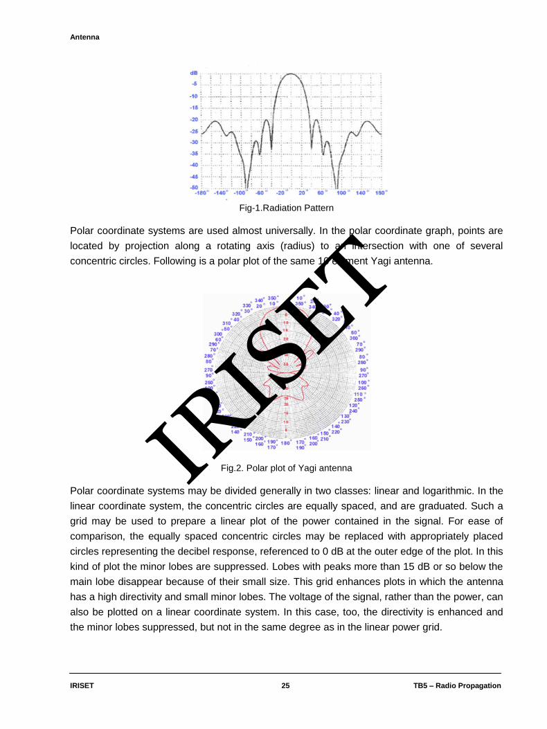
Fig-1.Radiation Pattern
Polar coordinate systems are used almost universally. In the polar coordinate graph, points are
located by projection along a rotating axis (radius) to an intersection with one of several
concentric circles. Following is a polar plot of the same 10 element Yagi antenna.
Fig.2. Polar plot of Yagi antenna
Polar coordinate systems may be divided generally in two classes: linear and logarithmic. In the
linear coordinate system, the concentric circles are equally spaced, and are graduated. Such a
grid may be used to prepare a linear plot of the power contained in the signal. For ease of
comparison, the equally spaced concentric circles may be replaced with appropriately placed
circles representing the decibel response, referenced to 0 dB at the outer edge of the plot. In this
kind of plot the minor lobes are suppressed. Lobes with peaks more than 15 dB or so below the
main lobe disappear because of their small size. This grid enhances plots in which the antenna
has a high directivity and small minor lobes. The voltage of the signal, rather than the power, can
also be plotted on a linear coordinate system. In this case, too, the directivity is enhanced and
the minor lobes suppressed, but not in the same degree as in the linear power grid.
IRIS
ET

Antenna
IRISET 26 TB5 – Radio Propagation
Fig.3. Shape of the beam
A modified logarithmic scale emphasizes the shape of the major beam while compressing very
low-level (>30 dB) side lobes towards the center of the pattern. There are two kinds of radiation
pattern: absolute and relative. Absolute radiation patterns are presented in absolute units of field
strength or power. Relative radiation patterns are referenced in relative units of field strength or
power. Most radiation pattern measurements are relative to the isotropic antenna, and then the
gain transfer method is then used to establish the absolute gain of the antenna.
The radiation pattern in the region close to the antenna is not the same as the pattern at large
distances. The term near-field refers to the field pattern that exists close to the antenna, while
the term far-field refers to the field pattern at large distances. The far-field is also called the
radiation field, and is what is most commonly of interest. Ordinarily, it is the radiated power that
is of interest, and so antenna patterns are usually measured in the far-field region. For pattern
measurement it is important to choose a distance sufficiently large to be in the far-field, well out
of the near-field. The minimum permissible distance depends on the dimensions of the antenna
in relation to the wavelength. The accepted formula for this distance is:
rmin = 2d2/
Where rmin is the minimum distance from the antenna, d is the largest dimension of the antenna,
and is the wavelength.
2.1.6. Beam width
An antenna's beam width is usually understood to mean the half-power beam width. The peak
radiation intensity is found and then the points on either side of the peak which represent half the
power of the peak intensity are located. The angular distance between the half power points is
defined as the beam width. Half the power expressed in decibels is —3dB, so the half power
beam width is sometimes referred to as the 3dB beam width. Both horizontal and vertical beam
widths are usually considered.
Assuming that most of the radiated power is not divided into side lobes, then the directive gain is
inversely proportional to the beam width: as the beam width decreases, the directive gains
increases.
IRIS
ET

Antenna
IRISET 27 TB5 – Radio Propagation
2.1.7. Nulls
In an antenna radiation pattern, a null is a zone in which the effective radiated power is at a
minimum. A null often has a narrow directivity angle compared to that of the main beam. Thus,
the null is useful for several purposes, such as suppression of interfering signals in a given
direction.
2.1.8. Polarization
Polarization is defined as the orientation of the electric field of an electromagnetic wave.
Polarization is in general described by an ellipse. Two special cases of elliptical polarization are
linear polarization and circular polarization. The initial polarization of a radio wave is determined
by the antenna.
With linear polarization the electric field vector stays in the same plane all the time. Vertically
polarized radiation is somewhat less affected by reflections over the transmission path. Omni
directional antennas always have vertical polarization. With horizontal polarization, such
reflections cause variations in received signal strength. Horizontal antennas are less likely to
pick up man-made interference, which ordinarily is vertically polarized.
In circular polarization the electric field vector appears to be rotating with circular motion about
the direction of propagation, making one full turn for each RF cycle. This rotation may be right
hand or left hand. Choice of polarization is one of the design choices available to the RF system
designer.
2.1.9. Polarization Mismatch
In order to transfer maximum power between a trans and a receive antenna, both antennas must
have the same spatial orientation, the same polarization sense and the same axial ratio.
When the antennas are not aligned or do not have the same polarization, there will be a
reduction in power transfer between the two antennas. This reduction in power transfer will
reduce the overall system efficiency and performance.
FIG.4. Polarity mismatched
IRIS
ET

Antenna
IRISET 28 TB5 – Radio Propagation
When the transmit and receive antennas are both linearly polarized, physical antenna
misalignment will result in a polarization mismatch loss which can be determined using the
following formula
Polarization Mismatch Loss (dB) = 20 log (cos)
Where is the misalignment angle between the two antennas. For 15° we have a loss of 0.3 dB,
for 30° we have 1.25 dB, for 45° we have 3 dB and for 90° we have an infinite loss.
The actual mismatch loss between a circularly polarized antenna and a linearly polarized
antenna will vary depending upon the axial ratio of the circularly polarized antenna.
If polarizations are coincident no attenuation occurs due to coupling mismatch between field and
antenna, while if they are not, then the communication can't even take place.
2.1.10. Front-to-back ratio
The front-to-back ratio is the ratio of the maximum directivity of an antenna to its directivity in the
rearward direction. For example, when the principal plane pattern is plotted on a relative dB
scale, the front-to-back ratio is the difference in dB between the level of the maximum radiation,
and the level of radiation in direction 180 degrees.
2.2. Types of Antennas
A classification of antennas can be based on:
2.2.1. Frequency and size
Antennas used for HF are different from the ones used for VHF, which in turn are different from
antennas for microwave. The wavelength is different at different frequencies, so the antennas
must be different in size to radiate signals at the correct wavelength.
2.2.2. Directivity
Antennas can be Omni directional, sectorial or directive. Omni directional antennas radiate the
same pattern all around the antenna in a complete 360 degrees pattern. The most popular types
of omnidirectional antennas are the Dipole-Type and the Ground Plane. Sectorial antennas
radiate primarily in a specific area. The beam can be as wide as 180 degrees, or as narrow as
60 degrees. Directive antennas are antennas in which the beam width is much narrower than in
sectorial antennas. They have the highest gain and are therefore used for long distance links.
Types of directive antennas are the Yagi, the biquad, the horn, the helicoidal, the patch antenna,
the Parabolic Dish and many others.
2.3. Isotropic antenna
Any signal that is transmitted by an antenna will suffer attenuation during its journey in free
space. The amount of power received at any given point in space will be inversely proportional
to the distance covered by the signal. This can be understood by using the concept of an
isotropic antenna. An isotropic antenna is an imaginary antenna that radiates power equally in all
directions. As the power is radiated uniformly, we can assume that a ‗sphere‘ of power is formed,
as shown in Figure 5
IRIS
ET

Antenna
IRISET 29 TB5 – Radio Propagation
Fig.5.Isotropic antenna
The surface area of this power sphere is:
A = 4π R2 The power density S at any point at a distance R from the antenna can be expressed as:
S =P*G/A
Where P is the power transmitted by the antenna, and G is the antenna gain. Thus, the received
power Pr at a distance R is:
Pr = P * Gt* G r (λ/4π R)2
Where Gt and Gr are the gain of the transmitting and receiving antennas and is the
wavelength respectively. On converting this to decibels we have:
Pr(dB) = P(dB) + Gt(dB) + Gr(dB) + 20log (λ/4π) − 20log d.
Last two terms are together called the path loss in free space, or the free space loss (FSL). The
first two terms (P and Gt) combined are called the effective isotropic radiated power (EIRP).
Thus: Free-space loss (dB) = EIRP + Gr(dB) − Pr(dB). The free-space loss can then be given as:
L dB = 32.4 + 20log f + 20log d
Where f is the frequency in GHz and d is the distance in km.
IRIS
ET

Antenna
IRISET 30 TB5 – Radio Propagation
Free Space Loss As signals spread out from a radiating source, the energy is spread out over a larger surface
area and the strength of that signal gets weaker. Free space loss (FSL), measured in dB,
specifies how much the signal has weakened over a given distance.
Fig.6.FSL in a radio link
Effective Isotropic Radiated Power Effective isotropic radiated power (EIRP) is the actual RF power as measured in the main lobe
(or focal point) of an antenna. It is equal to the sum of the transmit power into the antenna (in
dBm) added to the dBi gain of the antenna. Since it is a power level, the result is measured in
dBm.
Fig.6.EIRP of a radio
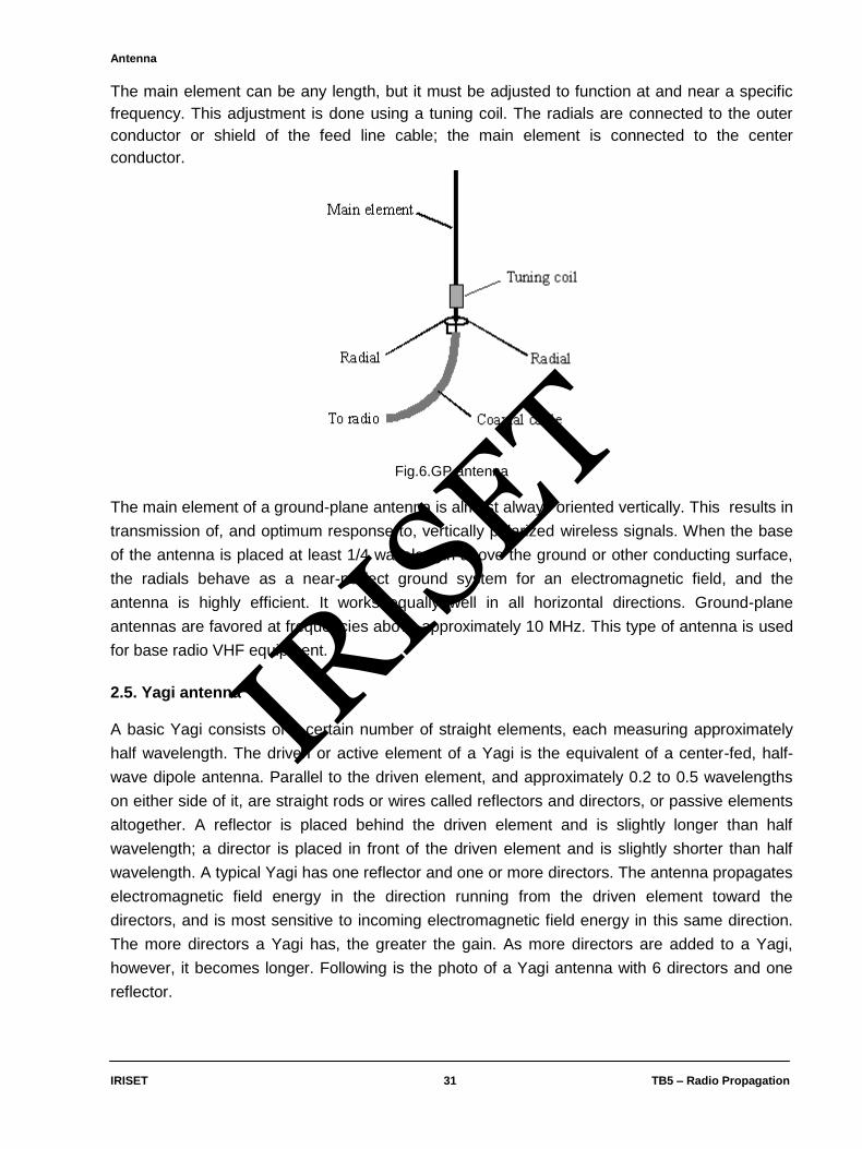
2.4. Ground-plane antenna A ground-plane antenna is a designed for use with an unbalanced feed line such as coaxial
cable. This antenna is designed to transmit a vertically polarized signal. It consists of a 1⁄4 wave
element as half-dipole and three or four 1⁄4 wavelength ground elements bent 30 to 45 degrees
down. This set of elements, called radials, is known as a ground plane. This is a simple and
effective antenna that can capture a signal equally from all directions.
IRIS
ET
Antenna
IRISET 31 TB5 – Radio Propagation
The main element can be any length, but it must be adjusted to function at and near a specific
frequency. This adjustment is done using a tuning coil. The radials are connected to the outer
conductor or shield of the feed line cable; the main element is connected to the center
conductor.
Fig.6.GP antenna
The main element of a ground-plane antenna is almost always oriented vertically. This results in
transmission of, and optimum response to, vertically polarized wireless signals. When the base
of the antenna is placed at least 1/4 wavelength above the ground or other conducting surface,
the radials behave as a near-perfect ground system for an electromagnetic field, and the
antenna is highly efficient. It works equally well in all horizontal directions. Ground-plane
antennas are favored at frequencies above approximately 10 MHz. This type of antenna is used
for base radio VHF equipment.
2.5. Yagi antenna A basic Yagi consists of a certain number of straight elements, each measuring approximately
half wavelength. The driven or active element of a Yagi is the equivalent of a center-fed, half-
wave dipole antenna. Parallel to the driven element, and approximately 0.2 to 0.5 wavelengths
on either side of it, are straight rods or wires called reflectors and directors, or passive elements
altogether. A reflector is placed behind the driven element and is slightly longer than half
wavelength; a director is placed in front of the driven element and is slightly shorter than half
wavelength. A typical Yagi has one reflector and one or more directors. The antenna propagates
electromagnetic field energy in the direction running from the driven element toward the
directors, and is most sensitive to incoming electromagnetic field energy in this same direction.
The more directors a Yagi has, the greater the gain. As more directors are added to a Yagi,
however, it becomes longer. Following is the photo of a Yagi antenna with 6 directors and one
reflector.
IRIS
ET

Antenna
IRISET 32 TB5 – Radio Propagation
. Fig. 7. Yagi antenna
Yagi antennas are used primarily for Point-to-Point links, have a gain from 10 to 20 dBi and a
horizontal beam width of 10 to 20 degrees.
2.6. Horn
The horn antenna derives its name from the characteristic flared appearance. The flared portion
can be square, rectangular, cylindrical or conical. The direction of maximum radiation
corresponds with the axis of the horn.
Fig.8. Horn antenna
2.7. Parabolic Dish
Antennas based on parabolic reflectors are the most common type of directive antennas when a
high gain is required. The main advantage is that they can be made to have gain and directivity
as large as required.
The main disadvantage is that big dishes are difficult to mount and are likely to have a large
wind age. The basic property of a perfect parabolic reflector is that it converts a spherical wave
irradiating from a point source placed at the focus into a plane wave. Conversely, all the energy
received by the dish from a distant source is reflected to a single point at the focus of the dish.
The position of the focus, or focal length, is given by:
IRIS
ET

Antenna
IRISET 33 TB5 – Radio Propagation
Where D is the dish diameter and c is the depth of the parabola at its center. The size of the dish
is the most important factor since it determines the maximum gain that can be achieved at the
given frequency and the resulting beam width. The gain and beam width obtained are given by:
Where D is the dish diameter and n is the efficiency. The efficiency is determined mainly by the
effectiveness of illumination of the dish by the feed, but also by other factors. Each time the
diameter of a dish is doubled, the gain is four times, or 6 dB, greater. If both stations double the
size of their dishes, signal strength can be increased of 12 dB, a very substantial gain. An
efficiency of 50% can be assumed when hand-building the antenna.
The ratio f/D (focal length/diameter of the dish) is the fundamental factor governing the design of
the feed for a dish. The ratio is directly related to the beam width of the feed necessary to
illuminate the dish effectively. Two dishes of the same diameter but different focal lengths
require different design of feed if both are to be illuminated efficiently. The value of 0.25
corresponds to the common focal-plane dish in which the focus is in the same plane as the rim
of the dish.
Dishes up to one meter are usually made from solid material. Aluminum is frequently used for its
weight advantage, its durability and good electrical characteristics. Windage increases rapidly
with dish size and soon becomes a severe problem. Dishes which have a reflecting surface that
uses an open mesh are frequently used. These have a poorer front-to-back ratio, but are safer to
use and easier to build. Copper, aluminum, brass, galvanized steel and iron are suitable mesh
materials.
2.8. Other Antennas
Many other types of antennas exist and new ones are created following the advances in
technology.
2.8.1 Sector or Sectorial antennas: they are widely used in cellular telephony infrastructure
and are usually built adding a reflective plate to one or more phased dipoles. Their horizontal
beam width can be as wide as 180 degrees, or as narrow as 60 degrees, while the vertical is
usually much narrower. Composite antennas can be built with many Sectors to cover a wider
horizontal range (multisectorial antenna).
A sector antenna is a type of directional microwave antenna with a sector-shaped radiation
pattern. The word "sector" is used in the geometric sense; some portion of the circumference of
a circle measured in degrees of arc. 60°, 90° and 120° designs are typical, often with a few
degrees 'extra' to ensure overlap and mounted in multiples when wider or full-circle coverage is
required.
IRIS
ET

Antenna
IRISET 34 TB5 – Radio Propagation
A 60 degree sector antenna covers 60 degrees (1/6) of a 360 degree circle, while a 90 degree
sector antenna covers a fourth of that same circle. The radiation areas don't end abruptly at 60,
90, or 120 degrees; these have a few degrees of overlap so you could, for example, use three
120 degree sector antennas for full coverage of a circle
The largest use of these antennas is for cell phone base-station sites. They are used for limited-
range distances of around 4 to 5 km.
Fig . 9 . Sector antenna
A typical sector antenna is depicted in the figure 9. At the bottom, there are RF connectors for
coaxial cable (feed line), and adjustment mechanisms. For its outdoor placement, the main
reflector screen is produced from aluminum, and all internal parts are housed into a fiberglass
radome enclosure to keep its operation stable regardless of weather conditions.
The antenna's long narrow form gives it a fan-shaped radiation pattern, wide in the horizontal
direction and relatively narrow in the vertical direction. According to the radiation patterns
depicted, typical antennas used in a three-sector base station has 66° of horizontal beam width.
This means that the maximum gain is achieved at 0° and its value is slightly low at the ±33°
directions. At the ±60° directions, it is suggested to be a border of a sector and antenna gain is
negligible there.
Fig.10 .Field pattern
Vertical beam width is not wider than 15°, meaning 7.5° in each direction. Which must achieve
line-of-sight over many miles or kilometers, there is usually a downward beam tilt or down tilt so
that the base station can more effectively cover its immediate area and not cause RF
interference to distant cells.
Coaxial cable
IRIS
ET

Antenna
IRISET 35 TB5 – Radio Propagation
The coverage area which is equal to the square of the sector's projection to the ground can be
adjusted by changing electrical or mechanical down tilts. Electrical tilt is set by using a special
control unit which usually is built into the antenna case and Mechanical down tilt is set manually
by adjusting an antenna fastener
Grounding is very important for an outdoor antenna so all metal parts are DC-grounded.
2.8.2. Whip antenna
A whip antenna is an antenna consisting of a single straight flexible wire or rod. The bottom end
of the whip is connected to the radio receiver or transmitter. They are designed to be flexible so
that they won't break off, and the name is derived from their whip-like motion when disturbed.
Often whip antennas for portable radios are made of a series of interlocking telescoping metal
tubes, so they can be retracted when not in use. Longer ones made for fixed mounting on
vehicles or structures are made of a flexible fiberglass rod surrounding a wire core, and can be
up to 35 ft (10 m) long. Whips are the most common type of monopole antenna. These antennas
are widely used for hand-held radios such as cell phones, cordless phones, walkie-talkies, FM
radios, boom boxes, Wifi enabled devices, and GPS receivers, and also attached to vehicles as
the antennas for car radios and two way radios for police, fire and aircraft attached to vehicles as
the antennas for car radios and two way radios for police, fire and aircraft.
Fig..11 .Whip antenna used for VHF sets
Multi-band operation is possible with coils at about one-half or one-third and two-thirds that do
not affect the aerial much at the lowest band but create the effect of stacked dipoles at a higher
band (usually x2 or x3 frequency).
2.9. Smart Antenna
A smart antenna is a digital wireless communications antenna system that takes advantage of
diversity effect at the source (transmitter), the destination (receiver), or both. Diversity effect
involves the transmission and/or reception of multiple radio frequency (RF) waves to increase
data speed and reduce the error rate.
In conventional wireless communications, a single antenna is used at the source, and another
single antenna is used at the destination. This is called SISO (single input, single output). Such
systems are vulnerable to problems caused by multipath effects. When an electromagnetic field
(EM field) is met with obstructions such as hills, canyons, buildings, and utility wires, the wave
fronts are scattered, and thus they take many paths to reach the destination. The late arrival of
IRIS
ET

Antenna
IRISET 36 TB5 – Radio Propagation
scattered portions of the signal causes problems such as fading, cut-out (cliff effect), and
intermittent reception (picket fencing). In a digital communications system like the Internet, it can
cause a reduction in data speed and an increase in the number of errors. The use of smart
antennas can reduce or eliminate the trouble caused by multipath wave propagation.
Smart antennas fall into three major categories: SIMO (single input, multiple output), MISO
(multiple input, single output), and MIMO (multiple input, multiple output).
In SIMO technology, one antenna is used at the source, and two or more antennas are used at
the destination.In MISO technology, two or more antennas are used at the source, and one
antenna is used at the destination. In MIMO technology, multiple antennas are employed at both
the source and the destination. MIMO has attracted the most attention recently because it can
not only eliminate the adverse effects of multipath propagation, but in some cases can turn it into
an advantage.
2.9.1. Smart Antenna – Functions
2.9.1. 1. Estimation of Direction of arrival (DOA)
In smart antennas various techniques like MUSIC (Multiple Signal Classification) and estimation
of signal parameters via rotational invariance techniques algorithms are used to find the DOA of
a signal. This method requires a lot of computations and algorithms.
2.9.1. 2. Beam forming Method
The mobiles or targets at which the signals are to be sent are first sought out and then a
radiation pattern of the antenna array is created by adding the signal phases. At the same time
the mobiles which will not need the signal will be out of pattern. Though this method may seem a
little too complicated, it can be done easily with the help of a FIR (Finite Impulse Response)
tapped delay line filter. According to the signal used the weight of the FIR filter can also be
changed accordingly. The filters will also be helpful in providing optical beam forming so as to
decrease the MMSE (Minimum Mean Squared Error) between the actual and wanted beam
pattern that is formed
2.9.2.Types of Smart Antennas
The classification of Smart Antennas depends on the type of environment and the requirements
of the system. There are mainly two types of Smart Antennas. They are
1. Phased Array/Beam Smart/Multi-beam Antenna
2. Adaptive Array Antenna
2.9.2.1 Phased Array/Beam Smart/Multi-beam Antenna
In this type of array, there will be numerous amount of fixed beams amongst which one beam
will turn on or will be steered towards the wanted signal. This can be done only with the help of
adjustment in the phase.
IRIS
ET

Antenna
IRISET 37 TB5 – Radio Propagation
Fig.12. Phased Array Antenna
2.9.2.2 Adaptive Array Antenna
In this type of antenna, there will be a change in the beam pattern according to the movement of
the wanted user and the movement of the interference. The signals that are received will be
weighted and later combined to increase the wanted signal to interference in addition to the
noise and power ratio [S/N]. Thus, the direction of interference will be balanced as the wanted
signal will be in the direction of the main beam.
The antenna can easily steer the main beam to any direction, while at the same time nullifying
the interfering signal. The direction of the beam can be calculated using the DOA method. The
figure of an adaptive array antenna is shown below
Fig.13. Adaptive Array Antennas
2.9.2.3. Advantages
Both beam smart and adaptive arrays provide high efficiency and thus high power for the
desired signal. When a large number of antenna elements are used at a higher frequency, Beam
Smart antennas use narrow pencil beams. Thus high efficiency is obtained in the direction of the
desired signal. If a fixed number of antenna elements are used the same amount times the
power gain will be produced with the help of adaptive array antennas.
Another advantage is in the amount of interference that is suppressed. Beam smart antennas
suppress it with the narrow beam and adaptive array antennas suppress the interference by
adjusting the beam pattern.
IRIS
ET

Antenna
IRISET 38 TB5 – Radio Propagation
2.9.2.4 Disadvantages The main disadvantages are 1. Cost: The cost of such a device will be more, not only in the electronics section, but also in
the power. That is the device is way too expensive [especially if MIMO methods are used.], and
will also decrease the life of battery of mobiles. The receiver chains that are used must be
reduced in order to reduce the cost. Also the costs rise up due to the RF electronics and A/D
converter used for each antenna.
2. Size: For this method to be efficient large base stations are needed. This will increase the
size. Apart from this multiple external antennas are needed on each terminal. This is not
practical. But companies re trying methods like dual polarization to reduce the size.
3. Diversity: When multiple mitigation is needed, diversity becomes a big problem. The
terminals and base stations must have multiple antennas. There are mainly three types of
diversities. They are spatial, polarization, and angle.
Spatial separation of the antennas that are used is practically impossible when it is applied on
mobile phones. It is also difficult to be achieved in point-to-point systems where a near line-of-
sight exists between the transmitter and receiver. By using polarized diversity, the above
problem can be avoided to a certain point. Dual polarization can be easily instigated without the
use of spatial separation.
Angular diversity is the most commonly used method nowadays. The signals which have the
maximum signal power are selected from multiple beams and are used to maintain diversity. But
the gain depends on the angular spread. That is, if the spread is small, the diversity will also be
small.
IRIS
ET

Annexure
IRISET 39 TB5 – Radio Propagation
ANNEXURE
FREQUENCY ALLOCATIONS AND FREQUENCY PLAN Indian Railways have been allotted a frequency band of 7125 MHz to 7425 MHz (4.21 cms -
4.04 cms wavelengths) in the Xc band. (The band of frequency from 7250 - 7300 MHz is
restricted in view of satellite to earth allotment). The spot frequencies permitted in the band for
operation of a transmitter (and Receiver) are governed by CCIR Recommendation 385 - 1 which
inter - alia stipulates as follows: -
fo = Center frequency = 7275 MHz
fn = Channel frequency in MHz in lower half of the band
f1n = Channel frequency in MHz in Upper half of the band.
Then the frequencies (MHz) of the individual channels are expressed by the following
relationships:-
Lower half of band fn = fo - 154 + 7n
Upper half of band f1n = fo + 7 + 7n
Where n = 1, 2, 3, etc., .upto 20. e.g., f1 = (7275 – 154 +7x1 ) =7128 MHz & f1
1 = (7275 +7 + 7x1) =7289 MHz
f2 =7135 MHz & f‘2 =7296 MHz and so on. In section over which the international conduction is arranged all the 'go' channels should be in
one half of the band and all the 'return' channels in the other half of the band.
When systems with 300 telephone channels are operated in a radio frequency band, channel
combination, which result in differences between channel frequencies of less than 14 MHz,
should in general be avoided. If sufficient antenna discrimination is available, this precaution
may be disregarded.
Frequency Plan There are two distinct patterns of frequency plans employed on the Railways. They are the 'Four
Frequency' and the 'Two Frequency' plans.
Characteristics of a four-frequency plan: Allocation of frequencies in a four frequency plan is
as shown in the Fig.1.
IRIS
ET

Annexure
IRISET 40 TB5 – Radio Propagation
Fig..1. Four Frequency Plan (100% Standby Equipment)
The transmit frequencies from A towards B and from B towards C are different so that there is no
chance of interference caused by radiation from A to B reaching Station C (or vice versa i.e. C to
B reading A). The signal from A meant for B and reaching C would be attenuated primarily by
Band Pass filter in the receiver at C and thus interference noise shall be effectively curtailed.
Similarly, signal from Station B towards C (frequency f3) going in the backward direction (i.e.,
towards A) is effectively attenuated by band pass filter in receiver at A which permits only f'7 to
pass in the rectifier section. It is possible therefore, to employ a standard performance antenna
with an F/B ratio of up to 45 dB. The four-frequency plan is, therefore, superior in as much as the
interference caused in the system is effectively controlled due to judicious use of different
frequencies. The price one pays for such improved performance is the use of more frequency
pairs. In the third hop, however, (i.e. transmission from C to D) the frequency f7 is repeated (to
conserve the frequency spectrum usage). No discussion on the four-frequency plan can be
complete without ref. to the 'radio equipment standby' vis-à-vis the frequency plan. Let us take
the case of Station B. The transmitter at B for direction BC is tuned for frequency f3 and for
direction BA is tuned to frequency f'7. The corresponding receivers are tuned for frequencies f'3
and f'7 and provide standby radio equipment at any Station to cater for improved system
reliability even in the face of component failure causing an equipment (a transmitter or a receiver
in this case) to fail. It should be obvious in this case that a separate transmitter tuned to radiate
on f3 for direction BC and a separate one of f'7 for direction BA shall be required as standby
transmitters. Similarly, separate receivers operating on f'3 and f'7 are required. Two standby
transmitter/receivers will thus be required for two working transreceivers.
A four-frequency plan thus needs 100% standby radio equipment. In a nutshell, it can be said
that a four-frequency plan causes less interference, permits standard antennae, but requires
100% radio equipment standby and of course necessitates larger pairs of frequencies.
IRIS
ET

Annexure
IRISET 41 TB5 – Radio Propagation
Characteristics of a two-frequency plan are: - 1) F/B interference is likely to be sizeable unless antenna of better F/B ratio (High performance
antenna with 65 dB F/B ratios) is employed. F/B interference refers to signal transmitted from
B in the direction of C that goes in the backward direction to A as noise.
2) Better utilization of frequencies achieved. 3) Standby radio equipment to the tune of only 50% is sufficient meaning thereby that one
transreceiver can be used as a standby for both the working transreceivers because the
transmit frequencies in both directions (e.g., B to C & B to A) are identical. Receive
frequencies from both directions (e.g. A to B and D to B) are also identical.
In the event of any component failure in transreceivers the standby transreceivers is
automatically switched over by the supervisory equipment that monitors the functioning of the
radio equipment.
The trade - off of the 'two frequency plan' is economy in radio equipment costs and better usage
of limited number of frequencies made feasible against the higher price to be paid for better
types of Antennae.
On India Railways a majority of the systems installed earlier employees a two-frequency plan
whereas recently there is a trend in favour of the four frequency plans.
FIG.2. Two-frequency plan (50% Stand by equipment)
IRIS
ET
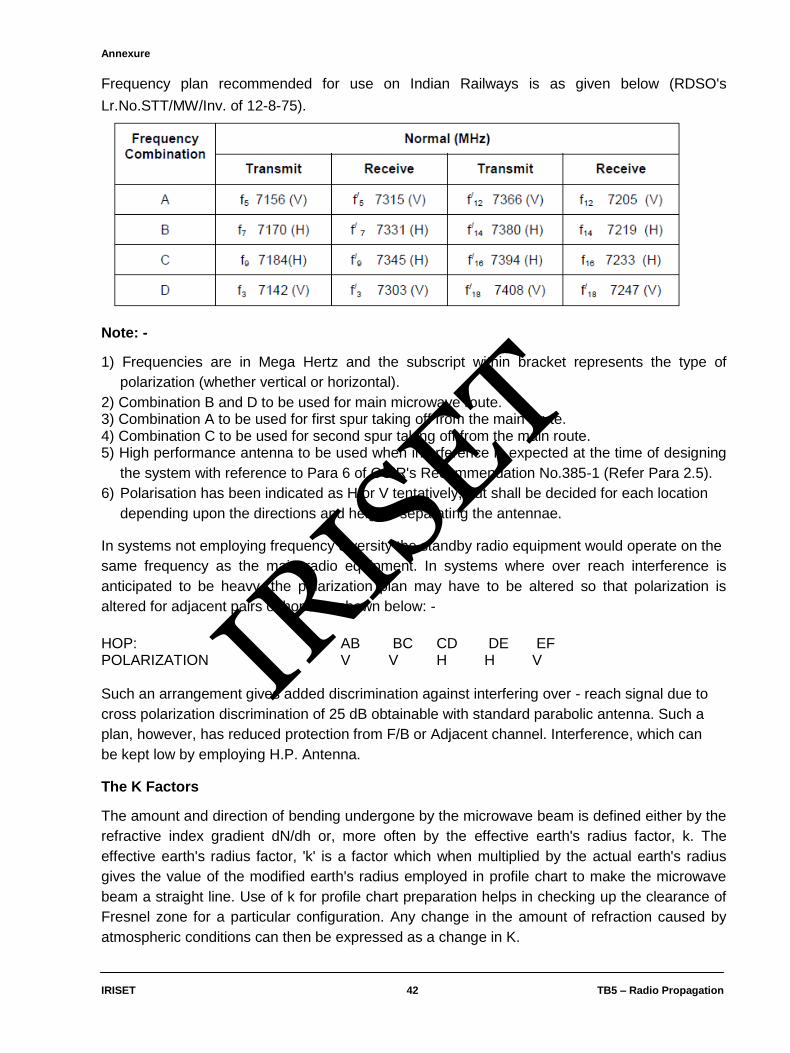
Annexure
IRISET 42 TB5 – Radio Propagation
Frequency plan recommended for use on Indian Railways is as given below (RDSO's
Lr.No.STT/MW/Inv. of 12-8-75).
Note: -
1) Frequencies are in Mega Hertz and the subscript within bracket represents the type of
polarization (whether vertical or horizontal).
2) Combination B and D to be used for main microwave route. 3) Combination A to be used for first spur taking off from the main route. 4) Combination C to be used for second spur taking off from the main route. 5) High performance antenna to be used when interference is expected at the time of designing
the system with reference to Para 6 of CCIR's Recommendation No.385-1 (Refer Para 2.5).
6) Polarisation has been indicated as H or V tentatively, but shall be decided for each location
depending upon the directions and heights separating the antennae.
In systems not employing frequency diversity the standby radio equipment would operate on the
same frequency as the main radio equipment. In systems where over reach interference is
anticipated to be heavy, the polarization plan may have to be altered so that polarization is
altered for adjacent pairs of hops as shown below: -
HOP: AB BC CD DE EF POLARIZATION V V H H V Such an arrangement gives added discrimination against interfering over - reach signal due to
cross polarization discrimination of 25 dB obtainable with standard parabolic antenna. Such a
plan, however, has reduced protection from F/B or Adjacent channel. Interference, which can
be kept low by employing H.P. Antenna.
The K Factors
The amount and direction of bending undergone by the microwave beam is defined either by the
refractive index gradient dN/dh or, more often by the effective earth's radius factor, k. The
effective earth's radius factor, 'k' is a factor which when multiplied by the actual earth's radius
gives the value of the modified earth's radius employed in profile chart to make the microwave
beam a straight line. Use of k for profile chart preparation helps in checking up the clearance of
Fresnel zone for a particular configuration. Any change in the amount of refraction caused by
atmospheric conditions can then be expressed as a change in K.
IRIS
ET

Annexure
IRISET 43 TB5 – Radio Propagation
The Atmosphere Blackout fading results from the formation of unusually steep, negative atmospheric density
gradients, a dramatic drop in humidity, or an increase in temperature with height, for example.
As the microwave beam is propagated through a blackout atmosphere, the lower part of the
wave front is allowed by the dense air with respect to the upper part, causing a tilting of the wave
front towards the ground or water. The amount of tilt is very small, but over a 20 mils distance
the amount of accumulated bending could refract the propagated beam into the ground before it
reaches the receive antenna. The beam may then be absorbed by foliage or crops, or scattered
by rough terrain, but in most often specularly reflected by smooth terrain, or water (in which case
it will re-appear again at greater distance).
Atmospheric density and refractive indexes are important in determining k factors for
establishing path clearances. The density of the atmosphere, in terms of its refractive properties,
is a function of pressure, temperature and humidity in the following approximate relationship.
N = 77.6 / T (P + 48 log10 e/T) Rec 453 CCIR.
Where N = Atmospheric refractive index (N-Units)
P = Pressure, millibars
T = Temperature, K (273 + C) 0
e = Saturation vapour pressure, millibars
Further K is given by, K = 157/(157 + dN/dh.) During standard atmospheric conditions, the range of k is from 1.2 in dry elevated areas and 4/3
in typical inland areas, to 2 or 3 in humid coastal area. The earth appears to become
increasingly flat as the value of k increases (). When k equals infinity the earth appears to a
microwave beam to be perfectly flat since the beam curves at exactly the same rate as the earth.
If the value of k becomes less than one, the beam curves upwards or opposite to the curvature
of the earth; to the microwave beam, the earth appears to "bulge". The effect of earth's bulge
may be to partially obstruct the transmission path, causing an obstruction or diffraction.
IRIS
ET

Annexure
IRISET 44 TB5 – Radio Propagation
Fig..3. Relation between K and microwave propagations
The curvature for various values of k can be calculated from the relationship: -
h = d1 d2/12.75 k. Where h = the change in vertical distance from a horizontal reference line in meters.
d1= the distance from a point to one end of the path in Kms.
d2= the distance from the same point as above to the other end of the path, in Kms., and
k = the effective earth's radius factor.
IRIS
ET

Annexure
IRISET 45 TB5 – Radio Propagation
Exempting multipath fading (easily overcome with diversity techniques), changes in k from 1 to
infinity have little influence upon the received signal level of a properly engineered microwave
path. Anomalous propagation occurs outside of this 'normal' range of k. With k less than 1, the
path could become obstructed and vulnerable to extreme multipath fading. When negative
values of k occur, the path may become trapped and susceptible to blackout fading
Super standard Refraction
Super standard refraction (also called super-refraction), results from such meteorological
conditions as a rise in temperature with increasing height (temperature inversion) or a marked
decrease in total moisture content in the air with increasing height, either of which will cause a
reduction in the atmospheric density with height. Under these circumstances, k increases,
resulting in a flattening of the effective earth's curvature.
One of the conditions that may cause this type of abnormal refraction is the passage of cool air
over warm body of water. Evaporation of the water will cause an increase in humidity and the
low temperature near the surface is a sign of a temperature inversion. Low temperature near the
surface is a sign of a temperature inversion. Low temperatures and high humidity greatly
increase the atmospheric density near the surface, causing an abnormally high do wire bending
of the wave-front. In moderate instances of super-refraction, k approaches infinity and a
microwave beam which is propagated parallel to the earth will remain parallel until obstructed or
otherwise attenuated. An extreme case of super refraction will bend the wave front downward
with a radius smaller than that of the earth (negative k), causing a blackout fade if the receiver is
beyond the point at which the wave front refracts into the ground (the radio horizon).
Sub-standard Refraction
Substandard or less than standard refraction occurs with certain meteorological conditions which
causes the atmospheric density to actually increase with height. This conditions, described
earlier as Earth's bulge or inverse than bending, causes an upward curvature of the microwave
beam, where k = 1/2. A sub-standard atmospheric condition may occur through the formation of
fog created with the passage of warm air over a cool air or a moist surface. This will cause the
atmospheric density to be lower near the ground than at higher elevations, causing an upward
bending of the beam.
M Profiles
The discussion of atmospheric irregularities is often aided by the use of another term or symbol,
M, which is called the 'modified' index of refraction. It is defined in terms of the radio refractive
index and the mean sea level elevation. The following formula is applicable: -
M = (n - 1) x 106 + 15.75h ... V.3 Where n = the radio refractive index.
h = the height above sea level in hundreds of meters.
IRIS
ET

Annexure
IRISET 46 TB5 – Radio Propagation
In the normal atmosphere (where K = 4/3), M increases at a linear rate of about a 11.8 units per
hundred meters increase in altitudes. When height is plotted as ordinate against M as abscissa,
the plot is called an M profile. The slop of the M profile determines the degree of bending of the
microwave beam in relation to the earth.
For discussion purposes it might be somewhat easier to follow a simplified equation for M. The
term N, which is the variable fraction of the refractive index, then becomes the parameter
against which the modified index M and its profile are compared.
The new equation becomes: M = N + 15.75h ... v.3
Illustrations of Refraction as Related to the M Profile
Figure 4 illustrates the M profile representing the "standard" condition, where K = 4/3 and the
slope of the profile is constant at3.6units per hundred meters.
Fig. 4 is a group of M profiles representing specific conditions that will be discussed in the
following paragraphs.
If N decreases more rapidly than normal increasing altitude, the slope of the M curve is steeper,
the value is greater than 4/3, and the microwave beam follows the curvature of the earth more
closely. If the value of M becomes constant with change in altitude, the microwave beam follows
curvature of the earth exactly, and K is equal to infinity.
IRIS
ET

Annexure
IRISET 47 TB5 – Radio Propagation
Fig..4. M profiles
This condition is represented graphically by a vertical M profile as shown for super-standard in
Fig. 4. It would be represented on a path profile by a flat earth and a straight-line microwave
beam. If conditions become even more extreme, the M profile will have a negative slope,
corresponding to a negative K, or a "concave earth" condition. An example of this condition is
the rare instance when an overreach interference signal is recorded at a station, and yet the
over reach path is obstructed by several hundred meters when the path profile is plotted on flat
earth.
When the slope of the M profile is greater than normal, the refractive, condition is referred to as
super-standard or earth flattening, since the radio horizon distance is increased. When the slope
of the M profile is less than normal, the refractive condition is known as sub-standard or earth
building. This condition is reflected in Fig. 4(b).
In practice, linear profiles do not usually occur except near the standard profile, because
whether factors usually change the shape of the M profile as well as its slope.
The effect of an abnormally high surface temperature, or increasing water vapour content with
altitude, is shown in the M profile of Fig.4(c). Such a sub-standard surface condition will result in
curving the beam away from the earth and this is called inverse beam bending or earth bulging.
The effect is similar to that from a linear M profile with a slope less than normal (earth bulging)
except that it is concentrated near the surface of the earth.
A rise in temperature with increasing height, or a decrease in water vapour content, or both, will
produce the effect shown in Fig. 4 (d). This is a slightly super-standard condition that will cause
the beam to follow the curvature of the earth more closely (earth flattening).
When the changes in refractive index are most severe near the surface, the condition will be as
shown in Fig. 4(e). This condition is known as a surface duct, because the beam will tend to stay
within the surface and the elevation limits; depending on the slope of the M profile near the
surface. When the beam enters the duct at a small angle, it is bent until it is horizontal and then
turned downward by further bending.
IRIS
ET

Annexure
IRISET 48 TB5 – Radio Propagation
Fig. 4(f) is the M profile of an elevated duct, the upper limit of which is formed by the upper limit
of the super-standard or inversion layer from a to b, and the lower limit by the sub-standard layer
from b to c. Under these conditions, the beam will tend to remain within the duct limits from a to
c, due to the bending toward the centre of the duct. Concentration of radio energy within a duct
will cause an increase in received signal when both the transmitting and receiving antennas are
within the duct. Obviously, this effect cannot be relied on for satisfactory propagation, because
the conditions producing it are subject to change. The terms trapping, super-refraction and
guided propagation are also employed to describe duct phenomena.
M profiles that are essentially linear are significant primarily because of their effect on path
clearance. The non-linear profiles, in addition to affecting path clearances, also give rise to
conditions leading to an atmospheric multipath effect.
Figs No. 3 show the profile charts drawn for values of k = 0.8 k = 1.33, k = 3.6 and k = 1. A look
at these graphs would indicate that for a given choice of antenna heights at station 'A' and
Station 'B', the existing obstructions in the path are likely to obstruct the microwave path when
the value of k is low which corresponds to sub refractive conditions. From this point of view, it is
important that the path is engineered in such a fashion, that at the lowest value of k for which the
system should function satisfactorily two-thirds of the first fresnel zone should be clear. As for
Indian Railways, Tc-10 specification stipulates that at k = 4/3, the full fresnel zone should be
clear at a low value k = 1 at least 2/3 of the fresnel zone is clear. It would thus to appreciate that
path engineering has to ensure that at low value of k the terrain and the profile chart examined
from the point of view of obstruction.
It would be observed that the obstruction in the intermediate terrain zone to be less important at
higher values of k. As a matter of fact, as K increases in magnitude the clearance available at
intermediate point tends to be higher and no serious cognizance is required to be taken from the
point of view of obstruction of the radiation and stability of adequate fresnel zone clearance. At
higher values of k, there exists greater probability of the reflected ray reaching the antenna after
reflection at an intermediate point. In the event of the terrain near the point of reflection being
highly reflective, e.g., river, marshy land, lake or irrigated land, the reflected ray can be strong
and can cause fading of the receiving signal. In view of this at higher values of k, the system
engineer has to evaluate the point of reflection, locate the point of reflection in the field, and
check up the reflection co-efficient that is likely to be prevalent in that area. In the event of
reflected ray being strong, the antenna heights should be modified to ensure that the reflected
ray does not reach the receiving antenna even up to the highest values of k at which we want
the path to be engineered. Such a situation can be maneuvered by judicious choice of antenna
height wherein one of the rays that in the event of being reflected is successfully obstructed by
natural obstruction. It would, therefore, be apparent that one of the important aspects in path
engineering considerations involves checking up of the path from the point of view of obstruction
and availability of adequate fresnel zone clearance at the low values of 'k' and checking of the
conditions of reflection and its being successfully obstructed by an obstruction at higher values
of 'k'.
IRIS
ET


