
IMAGE QUALITY THROUGH THE ATMOSPHERE
Item Type text; Dissertation-Reproduction (electronic)
Authors Metheny, Wayne Warren, 1933-
Publisher The University of Arizona.
Rights Copyright © is held by the author. Digital access to this materialis made possible by the University Libraries, University of Arizona.Further transmission, reproduction or presentation (such aspublic display or performance) of protected items is prohibitedexcept with permission of the author.
Download date 19/07/2018 12:32:14
Link to Item http://hdl.handle.net/10150/289428

INFORMATION TO USERS
This material was produced from a microfilm copy of the original document. While the most advanced technological means to photograph and reproduce this document have been used, the quality is heavily dependent upon the quality of the original submitted.
The following explanation of techniques is provided to help you understand markings or patterns which may appear on this reproduction.
1.The sign or "target" for pages apparently lacking from the document photographed is "Missing Page(s)". If it was possible to obtain the missing page(s) or section, they are spliced into the film along with adjacent pages. This may have necessitated cutting thru an image and duplicating adjacent pages to insure you complete continuity.
2. When an image on the film is obliterated with a large round black mark, it is an indication that the photographer suspected that the copy may have moved during exposure and thus cause a blurred image. You will find a
good image of the page in the adjacent frame.
3. When a map, drawing or chart, etc., was part of the material being photographed the photographer followed a definite method in "sectioning" the material. It is customary to begin photoing at the upper left hand corner of a large sheet and to continue photoing from left to right in equal sections with a small overlap. If necessary, sectioning is continued again — beginning below the first row and continuing on until complete.
4. The majority of users indicate that the textual content is of greatest value, however, a somewhat higher quality reproduction could be made from "photographs" if essential to the understanding of the dissertation. Silver prints of "photographs" may be ordered at additional charge by writing the Order Department, giving the catalog number, title, author and specific pages you wish reproduced.
5. PLEASE ftiOTE: Some pages may have indistinct print. Filmed as received.
Xerox University Microfilms 300 North Zeeb Road Ann Arbor, Michigan 48106
76-22,483
METHENY, Wayne Warren, 1933-IMAGE QUALITY THROUGH THE ATMOSPHERE.
The University of Arizona, Ph.D., 1976 Physics, optics
Xerox University Microfilms, Ann Arbor, Michigan 48106

/ 1
IMAGE QUALITY
THROUGH THE ATMOSPHERE
by
Wayne Warren Metheny
*
A Dissertation Submitted to the Faculty of the
COMMITTEE ON OPTICAL SCIENCES (GRADUATE)
In Partial Fulfillment of the Requirements For the Degree of
DOCTOR OF PHILOSOPHY
In the Graduate College
THE UNIVERSITY OF ARIZONA
19 7 6

THE UNIVERSITY OF ARIZONA
GRADUATE COLLEGE
I hereby recommend that this dissertation prepared under my
direction by Wayne Warren Methenv
entitled Image Quality through the Atmosphere
be accepted as fulfilling the dissertation requirement of the
degree of Doctor of Philosophy
Dissertation Director Date
After inspection of the final copy of the dissertation, the
follov/ing members of the Final Examination Committee concur in
its approval and recommend its acceptance:''*
This approval and acceptance is contingent on the candidate's adequate performance and defense of this dissertation at the final oral examination. The inclusion of this sheet bound into the library copy of the dissertation is evidence of satisfactory performance at the final examination.

STATEMENT BY AUTHOR
This dissertation has been submitted in partial fulfillment of requirements for an advanced degree at The University of Arizona and is deposited in the University Library to be made available to borrowers under rules of the Library.
Brief quotations from this dissertation are allowable without special permission, provided that accurate acknowledgment of source is made. Requests for permission for extended quotation from or reproduction of this manuscript in whole or in part may be granted by the head of the major department or the Dean of the Graduate College when in his judgment the proposed use of the material is in the interests of scholarship. In all other instances, however, permission must be obtained from the author.
SIGNED

PREFACE
This dissertation covers the theoretical justification and the
theoretical analysis of an experiment for the measurement of image qual
ity through the atmosphere for a down looking, airborne camera. The
study is presented in a more general framework than that one experiment;
the justification made applies to other experiments as well, and the — -
calculation techniques presented are more widely applicable. But in
the analysis of the detailed error sources it is necessary to choose a
specific application, and the down looking, airborne camera is the
specific application here.
The airborne experiment is in fact now being conducted by the
Optical Sciences Center, The University of Arizona, Air Force Contract
F33615-74-C-1088. The experiment is much larger than this disserta
tion and involves a large team of scientists and technicians at the
Center which include this writer. It is in the nature of things that
a PhD dissertation must be independent work so that this report, with
respect to the experiment as a whole, represents a chunk of independent
work broken off from the rest. This has not been difficult to do; the
study stands logically by itself, and should be presented in about this
form even without PhD motivation.
The ground test results presented in Chapter 7, of necessity,
implicitly include an enormous amount of work done by others, but the
main intent of Chapter 7 is to give practical illumination to the
iii

iv
theoretical aspects of the problem. The results in Chapters 3 and 7
required computer programming for their generation, not done by the
author. The only other experimental results reported are in Chapter 6
on the various polarization properties of the receiver. They were based
upon fabrication and testing done almost exclusively by this writer, but
here also, the value to this report of the work lies in the insight it
gave to the theoretical analysis (and it gave many deep insights!).
Theso acknowledgments are longer than is usual, but even so, I
have found it impossible to do them justice. First in line come my
fellow team members on the airborne image quality ejqperiment currently
under way at the Optical Sciences Center, The University of Arizona.
They are Professor R. R. Shannon (Principal Investigator and my disserta
tion director), who first presented to me the two point source measure
ment concept; Dr. W. S. Smith (Project Manager), who I believe could
move the Earth without a lever or a place to stand if'that were what was
required; Don Hillman, R. B. Philbrick, C. Ceccon, and M. Arthur. I
could not sort out all the ideas, valuable to me, which were interchanged
on this project if I tried; I am not trying. There is a magic associated
in working on this team that I appreciate even more than the ideas.
(It has to be magic! How else could you explain all those 20-hour days?).
I have received aid from outside the team, too. Project Monitor,
R. Gruenzel, whose habit of refusing to buy a weak argument has been
very useful to me. Faculty members at the Center have made significant
contributions. Especially Dr. R. Shack, who trumped my two-channel

polarization receiver with a six-channel version, entending the measure
ment concept to include the pupil function itself, in addition to the
transfer function. Dr. Shack, Dr. A. S. Marathay, Dr. J.. Burke, and
Dr. J. Wyant provided very useful discussions. Dr. J. Gaskill described
in advance the great difficulties to be encountered in such an
experiment, so that when the time came, I had no right to be surprised.
Dr. F. Turner provided the expertise needed for the non-polarizing beam
splitters .
Last in line for acknowledgment come my fellow students; students
I have learned, always come last, but, in an institution such as this,
it is among the students that the ideas are often really hammered out.
The hammerers who have removed the most dents are E. Hawman and (former
student) V. Mahajan at the blackboard. L. Brooks showed me a trick or
two in the lab. P. Cheatham and R. Wagner had helpful contributions
and criticisms.

TABLE OF CONTENTS
Page
LIST OF ILLUSTRATIONS ix
LIST OF TABLES X
ABSTRACT xi
1. INTRODUCTION 1
Image Quality with Time Varying Wavefronts 2
2. OPTICAL PROPAGATION THROUGH TURBULENCE 14
Index of Refraction Statistics 16 Wave Front Statistics (Plane Waves) 19 Spherical Waves 23 Non-homogeneous Path 24 Vertical Path 24 Application Wavefront Statistics to Image Quality 25 Reciprocity 29
3. MODELING ATMOSPHERIC IMAGE QUALITY 31
Modeling the Outer Scale 31 Intermediate Exposure Time ATF 39 Sample Wavefronts from the PSD 40 Vertical Path Temporal Statistics 42 Model Results for the ATF 44
4. MEASUREMENT OF IMAGE QUALITY: REVIEW AND GENERAL CONSIDERATIONS 50
Point Spread Function Measurement 51 Geometrical Measurement 52 Interference Techniques 53 New Techniques 60
5. APPLICATION OF THE TWO POINT SOURCE TECHNIQUE TO THE MEASUREMENT OF THE TRANSFER FUNCTION 64
Experiment.Descriptions . ...... 65 Airborne Experiment 65 Fixed Path, Rotating Transmitter Experiment 66
vi
vii
TABLE OF CONTENTS—Continued
Page
Fixed Path, Fixed Transmitter Experiment . . . 67 System Design 67
Transmitter 67 Receiver 70 Signal-to-noise Ratio 70 Heterodyne Term 75 Rotating Transmitter 75 Translating Transmitter 78 Pockel's Cell Case 79 Data Reduction 81 Analog Formulation 81 Digital Formulation 83 Error Sources 86 Unequal Beams 87 Gaussian Beams 87 Non-straight Line Fringes 88 Alignment and Aberration Errors (Non-overlap) 91 Receiver Size 94 Data Reduction Errors 95 Heterodyne Error 95 Separation Error 96 Selection of u 101 Pitch Error 103
6. APPLICATION OF THE TWO POINT SOURCE TECHNIQUE TO THE MEASUREMENT OF THE PUPIL FUNCTION 106
Ideal Experiment 208
Ideal Transmitter 110 Ideal Receiver 113
4-Channel Experiment 117 Error Analysis 119
Non-ideal Transmitter 119 Non-ideal Receiver 120 Non-polarizing Beamsplitter 121 Ai2 and A22 Channels 125 Interference Channels 130
7. GROUND EXPERIMENTS 139
Transfer Function Experiment 139 Pupil Function Experiment 146

viii
TABLE OF CONTENTS—Continued
Page
8. CONCLUSIONS AND RECOMMENDATIONS 151
APPENDIX I: THE SEPARATION OF THE OPTICAL TRANSFER IN A TURBULENT MEDIUM 154
Qualitative Remarks 154 Weak Turbulence 158 Strong Turbulence 159 Frozen Wavefronts 160 Separation in Y-Direction due to Small Optical Aberrations 161
REFERENCES 163
LIST OF ILLUSTRATIONS
Figure Page
1. CM2 Profiles 34
2. Outer Scale Profile 36
3. Long Exposure Time ATF for Various Outer Scale Profiles . . 38
4. Model ATF for Both Amplitude and Phase Variations 46
5. Model ATF for Moderate Amplitude Variations 46
6. Model ATF for Small Amplitude Variations 47
7. Variation of Model Transfer Factors with Exposure Time ... 47
8. Model ATF vs. Turbulent Strength Parameters . . 49
9. System Design 68
10. Heterodyne Term Geometry 76
i 11. Heterodyne Error 97
12. Separation Error ; . . . 100
13. Error in Selection of u . . 102
14. Ideal Transmitter Ill
15. Three Prism Configurations 116
16. Condensed Data Output 141
17. Condensed Fourier Transform Computer Output 143
18. Measured Short Exposure ATFs shown with Theoretical Curves (after Lutomirski and Yura, 1971b) 145
19. Roof Transmitter 148
20. Phase Difference, Stationary Transmitter 150
ix

LIST OF TABLES
Table Page
1. Noise Parameters . 73
2. Signal Level Parameters 75
x

ABSTRACT
The optical image quality is developed in terms of the optical
transfer function (OTF), the point spread function (psf) and the pupil
function for a camera with time varying wavefronts due to atmospheric
turbulence. The conditions for separating the OTF into an independent
atmospheric part (ATF) and an optical system part are extended beyond
the conditions previously found in the literature and extended with the
aid of Taylor's hypothesis to cover intermediate time exposures. A mea
surement technique using a two point source transmitter is developed
from fundamental considerations which can be applied to the measurement
of the ATF or the atmospheric pupil function. The specific application
of a down looking, airborne camera is chosen for a detailed error analysis
of the technique. A ground test over a 3.5 mile and a 600 foot horizon
tal path is described. Calculations of the ATF for various geometries
is considered. Both long exposure time calculations (using a new model
of the outer scale) and intermediate exposure time calculations (using
computer generated sample wavefronts) are made.
xi

CHAPTER 1
INTRODUCTION
The image quality of an optical system is degraded when it
operates in a medium which has refractive index inhomogeneities. The
phase and amplitude of the wavefront in the entrance pupil is modulated.
The resulting image no longer depends only on the quality of the optical
system, but also upon the amount of distortion and modulation of the
wavefront. In the atmosphere, the refractive index inhomogeneities are
caused by temperature variations which are distributed by turbulent
action. The situation is compounded by the fact that the wavefront per
turbations are time varying; in many practical cases, the wavefront
changes during exposure time. This adds a new dimension to the problem:
the amount of data required to measure image quality in the atmosphere
can be much greater than in the optical testing laboratory.
Few attempts have been made to measure image quality in the
atmosphere without simplifying the problem in some way; either measure
ments have been made which apply to the specific optical system used
(and with results which cannot be applied to other optical systems) or
measurements have been made only with very long time exposures yielding
average data which, while applicable to other optical systems, tell
nothing about the intermediate time exposures. The same statement can
be made about attempts to calculate image quality as well as to measure
it. The purpose of this study is to produce and test a technique for

2
the measurement and calculation of image quality which is suitable for
intermediate exposure times and which is a measure of the atmosphere
only, and hence can be applied to any optical system.
The calculations of image quality are included in Chapter 3, and
two measurement techniques are developed in Chapters 5 and 6; one using
the transfer function, and one using the pupil function. Both the cal
culations and the measurements use a simplification to reduce the amount
of data required; the atmospheric perturbations at two points in the
aperture only (not the full aperture) are used to describe the image
quality degradation. This simplification is not universally applicable,
but it does apply especially well to an airborne, down-looking camera.
Consequently, the equipment designed and constructed for the experimen
tal techniques was tailored to this application. The testing of the
techniques, however, was conducted over a horizontal path (Chapter 7)
with such short time exposures that the two point simplication was not
justified. Thus, while the equipment testing was successful, the data
collected are probably not directly applicable to the image quality over
the test path.
Image Quality with Time Varying Wavefronts
The linear theory of image formation (without time varying wave-
fronts) is well developed and is the point of departure for this study.
In this chapter time varying wavefronts are added to the theory. Sim
plifications and all important concepts used later are introduced here.
Incoherent optical image formation ideally is a linear, shift
invariant system which transforms the intensity distribution of the

3
object 0(x,y) into the intensity distribution of the image, I(x,y):
where psf(x,y) is the so-called point spread function, impulse response,
or Green's function of the system.
tion is the optical transfer function, OTF (Nx,Ny), a function of the
spatial frequencies Nx and Ny. The convolution theorem implies:
where the tilde is used to indicate the Fourier transforms of I(x,y)
and 0(x,y).
The pupil function, p(x,y), is defined as the wave amplitude
distribution in the exit pupil of a system with a point source object
and is related to the psf and OTF. The exit pupil is a spherical sur
face whose center is the "image" point. Using the Fresnel diffraction
integral to propagate the wave amplitude disturbance from the exit pupil
to the image plane, one can easily show that the result is the Fourier
transform of the pupil function evaluated at Nx = Ny = .
where R is the radius of curvature of the exit pupil. Since the psf is
the modulus squared of the wave amplitude distribution in the image
plane it follows that
00
0(a,6) psf(x - a) y - g)dadg ( 1 - 1 )
The two dimensional Fourier transform of the point spread func-
I(Nx,Ny) = e(Nx,Ny)OTF(Nx,Ny) (1.2)

4
psf(x,y) F.T. p(x,y) 2 ',
CI. 3)
The convolution theorem then implies the following OTF: 00 00
OTF(Nx,Ny) = | jjpCx - y - ^r)p*Cx + y + ^)dxdy Ax = XRN
x
Ay = XRN. y(1.4)
where B is a normalization constant such that the OTF is unity at
Nx = Ny =0 and the superscript asterisk indicates the complex con
jugate. The integrand is called the sheared pupil function throughout
this report.
bulence quite naturally have been centered upon the image plane and
describe the effects on a point image, of the psf (Shack, 1967).
Motion of the centroid of the psf is called image dance or agitation.
Spreading of the psf is image blooming or image blur. Fluctuation in
the total power in the psf is scintillation. By Parseval's theorem the
total power in the exit or entrance pupil is the same as the total
power in the psf, but in this report the term scintillation is loosely
applied to any variation of intensity in the wavefront and not restricted
to the integral over the pupil.
three functions psf(x,y), OTF(Nx,Ny.) or p(x,y), although the last has
some claim to primacy since the point spread function and the optical
Phenomenological classification of the optical effects of tur-
The image quality may be specified equally well by any of the

5
transfer function may be derived from the pupil function but the pupil
function cannot be derived from either of the others. The pupil func
tion is a logical starting point for studying image quality through a
turbulent atmosphere since the pupil function always separates into an
atmospheric factor and an optical system factor. With no atmospheric
perturbation, the pupil function depends only on the optical system
and is expressed here with a subscript, q* •'•n terms of its modulus and
phase, the optical system pupil function is as follows:
PoO,y) = A (x,y)el2lrW(x,y) C1,5)
The aberration function W(x,y), is given by
W(x,y) = i[OPD(xc,yc) - OPD(x.y)] (1.6)
where X = wavelength
OPD(x,y) = Optical path difference between the entrance and exit
pupiIs.
OPD(xc>yc) = Optical path difference between the entrance and exit
pupils for the chief ray.
That is, an unperturbed wavefront from a point source is spherical in
the entrance pupil and deviates from a spherical wave when it reaches
the exit pupil by an amount depending on the optical system aberrations.
I The modulus Ao(x,y) is usually a binary function which specifies the

6
physical extent of the exit pupil but which may also include a spatial
variation of amplitude transmission fapodization).
When the wavefront is perturbed by the atmosphere the pupil
function becomes
P(x4yjt) = Ar (x,y ;t)e1( Cx'y;t)pQ(x,y) (1,7)
where A1 (x,y) and <j>'(x,y) are the modulus and phase of the perturbed
wave in the exit pupil apart from the optical system aberrations. This
equation clearly shows the pupil function separating into an atmosphere
part (time varying) and an optical system part (non-time varying). The
primes are used to indicate that the spatial variation of modulus and
phase are in the exit pupil reserving the unprimed spatial variations
A(x,y) and <j>(x,y) for referring to the entrance pupil. The entrance
pupil is the proper place to refer measures of the amplitude and phase
variations in order to be independent of any particular optical system;
there is at most a spatial magnification of coordinates between entrance
and exit pupils [apart from the aberrations already incorporated in
p0(x,y)] which in no way changes image quality.
For an instantaneous exposure or for an exposure time short with
respect to the temporal changes of the pupil function the perturbed wave-
front (or entrance pupil function) A(x,y;t)e^specifies the
effect of the atmosphere for any optical system and can be expressed in
terms of the psf or OTF for a specific optical system through the
equations given above. For a non-instantaneous exposure a time integra
tion is required, but not an integration of the pupil function. Optical

7
detectors are square law devices, located, of course, in the image plane.
The output of a square law detector in the image plane is proportional
to the image intensity for, more correctly, the irradiance). Therefore,
the point spread function is the proper function to integrate. The
effective psf for an exposure time, T, at time t is then proportional
to the time averaged psf during the exposure:
The effective optical transfer function is by definition the Fourier
transform of the effective psf; then, since the psf is bounded, the
order of integration may be interchanged (i.e., the time integration
may be performed after the spatial integration in the Fourier transform)
and the effective OTF is proportional to the time average (weighted by
scintillation or the total power fluctuations) of the instaneous OTF.
If the order of integration is again interchanged (same justification)
then the effective OTF may be written as
(1 .8)
t
OTF(N ,N ;t,T)
dt Po(x - y - -^)Po(x y + ^)dydx
(1.9)
Ax = ARN x
Ay = ARN y

8
The modulus squared operation and the autocorrelation operation
Cby which the psf and OTF were related to the pupil function) are
irreversible operations. This fact stymies an attempt to define a
unique "effective pupil function" from the time integrated OTF and psf.
And in fact it is clear that the time averaged pupil function has no
relation to image quality, for the phase perturbations tend to zero in
a long time average falsely implying improved image quality.
The specification of image quality by means of the pupil function
requires more data in a time vaiying medium than is required using the
OTF or psf, but it has the advantage that it always separates into an
atmospheric part and an optical system part. The sheared pupil function
clearly separates also, and it can serve equally well to specify image
quality. In fact the atmospheric part of the sheared pupil function and
the atmospheric part of the pupil function are related by an analytic
transformation; a one-dimensional transformation developed by Gruenzel
(1972) plays a prominent part in the management of the pupil function
discussed in a later chapter.
If the OTF were to separate, then there could be some advantage
to treating the OTF instead of the pupil function. The only condition
found in the literature for OTF separation in a turbulent medium is for
' a time average sufficiently long such that it tends toward an ensemble
average, assuming that the atmospheric perturbations are formed by an
ergodic stationary random process (O'Neill, 1963). Other conditions
for OTF separation are given in Appendix I; they include a weak turbu
lence condition, a strong turbulence condition, and a partial separation

9
based upon Taylor's hypothesis (Taylor, 1958). Taylor's hypothesis
states that the temporal changes in atmospheric perturbations are domi
nated by the wind component perpendicular to the direction of propaga
tion; that is, during the time it takes the wind to sweep the disturbance
past the aperture, the atmospheric perturbations are "frozen" or rela
tively unchanged. The frozen atmosphere hypothesis, if not universally
applicable, is very frequently an accurate representation in practical
situations. The partial separation of the OTF due to Taylor's hypothesis
applies to all levels or strengths of turbulence and greatly enhances the
prospect of measuring the OTF of the atmosphere alone. Thus the OTF of
an arbitrary optical system operating in the atmosphere may be written
OTF(Nx,Ny;t,T) = ATF(Ax, Ay;t,T) OTFn(N ,N ) O* - x' y J
XRN Ax '
Ay = XRN (1.10)
L M
where M is the entrance to exit pupil magnification, OTFq is the optical
transfer function of the optical system alone, and the ATF or "atmo
spheric transfer function" is defined as the sheared atmospheric wave-
front averaged in time and averaged across the entrance pupil. It is
convenient to leave the ATF in terms of Ax, Ay in the entrance pupil,
and not evaluated in terms of Nx,Ny since these latter refer to a partic
ular optical system.
Separation of the transfer function also has an important effect
on the amount of data required from a measurement. Separation due to

10
the frozen atmosphere hypothesis implies that it is unnecessary to mea
sure the transfer function over the whole sheared aperture in one dimen
sion; measuring at one position along the wind direction is sufficient.
To a lesser extent the transfer function is also only weakly dependent
on y with the frozen atmosphere (see comments in Appendix 1) so that
measuring the transfer function at one point in the sheared aperture
(as a function of time) is sufficient.
It is also sufficient to measure the pupil function at one point
only in the aperture, although the justification is somewhat different
(and stronger) . The yaeasurement at one x position in the aperture is
justified in the same way as above, by Taylor's hypothesis. In the x
direction, using one point only (as a function of time) is sufficient
to generate one dimensional statistics of the pupil function which,
assuming homogeneity and isotropy, are easily converted to two dimen
sional statistics. Then computer generated sample wavefronts (two
dimensional) can be used to investigate the effects of time exposures
of any duration.
Computer generated sample functions are also useful in calcula
ting image quality based upon theoretical analysis of wavefront propa
gation through turbulence. The theoretical treatments which have been
applied to the problem are reviewed in Chapter 2. Of necessity,
ensemble averages are always used in analysis. In Chapter 3 theoreti
cal ensemble averages are used as the basis for one-dimensional sample
functions leading to calculations of the transfer function. Thus for
Chapter 3 (as well as Chapter 5), the one dimensional justification for

11
the transfer function must be invoked (suppressing for convenience the
time dependence of the ATF):
ATF (Ax) = f Ai(t)A2(t)e1" *2 (t) ldt J0
where Ai(t) = A(x -
A2(t) . = A(x + ,t) (1.11)
<h(t) = = <t>Cx - ±f.t)
<h(t) = = <j>(x + M t) 2
When the exposure time is sufficiently long the time average
converges to the ensemble average, assuming that the perturbations are
caused by an ergodic stationary random process. The atmospheric effects
may rarely or even never be truly represented by such a homogeneous
random process and in any event the time required is too long to be of
interest for intermediate exposure times. In the literature when the
ATF is an ensemble average then it is called variously the atmospheric
MTF (modulation transfer function) or the MCF (mutual coherence function),
or (more correctly), the mutual intensity function.
A review of the measurement techniques which have been reported
in the literature together with a general discussion of experimental
problems is given in Chapter 4. The output of a shearing interferometer
is closely related to the sheared pupil function and forms the basis for
the measurement of the OTF in Chapter 5 and of the pupil function in
Chapter 6. The output of a shearing interferometer which samples only
two points in a spherical wave after passing through turbulence is as
follows:

12
S(t) = Aj2(t) + A22(t) + 2Ai(t)A2(t)cos(b + A<Ji(t))
where A<j>(t) = - <j>2(t)
b - iirAx (1.12) X h X
h = radius of the spherical wave.
Except for the constant, b, the cosine term is the sheared pupil
function plus its complex conjugate. The constant b however, is access
ible to experimental modulation and can be used to heterodyne the cosine
term, separating it in frequency space from its complex conjugate and
Ai2 + A22. Time integration then gives the ATF for intermediate time
exposures.
In one particular applicaton, measuring the ATF for an airborne
downlooking camera, the motion of the aircraft itself provides the
heterodyning action. As a further advantage the motion of the aircraft
supplies a high velocity psuedo-wind which extends the application of
Taylor's theorem to shorter time exposures than could otherwise be
achieved. This particular application is analyzed in detail in
Chapter 5.
Measuring the pupil function is more complicated since the argu
ment A<j> is difficult to isolate from the shearing interferometer output.
In Chapter 6 a technique using multiple simultaneous outputs, each with
a different phase constant b, is presented which permits easy solution
of Ac|>.

13
For a variety of experimental reasons it is easier to run the
shearing interferometer backwards, taking advantage of the reciprocity
of light propagation in a turbulent medium. That is, instead of using
a point source, propagating it through the atmosphere, shearing the
resulting wavefront and superimposing the two components on a square
law detector, exactly the same output can be achieved by using two
mutually coherent point sources in the "entrance pupil" (now imaginary)
and propagating both beams backwards through the turbulent medium to a
point detector. Reciprocity is briefly discussed in Chapter 2. Recip
rocity is an old concept in diffraction theory (Goodman, 1968) but the
extension of the proof to a turbulent medium is of fairly recent origin
(Lutomirski and Yura, 1971b).

CHAPTER 2
OPTICAL PROPAGATION THROUGH TURBULENCE
The plan of this chapter is to present the results and applica
tions of the theory of propagation through turbulence which have been
reported in the literature. New applications of the theory and investi
gation of the validity of some applications is discussed in the next
chapter.
The theory of propagation through turbulence is not yet in
satisfactory form. Historically, the approaches used to study it over
the past twenty years parallel the approaches in non-turbulent optical
propagation theory over the past three hundred years. Geometrical tech
niques (ray optics) have been applied (Chandrasekar, 1952) to derive
the statistics of the wavefront. The wave equation for a turbulent
medium has been solved using approximations (Chernov, 1960; Tatarski,
1961). The double wave equation for the mutual coherence function (MCF)
has been used (Beran, 1967, 1970; Beran and Whitman, 1971; and Beran
and Ho, 1969). In addition, integral equation techniques have been
applied to both the wave amplitude propagation and the mutual coherence
function propagation. The Fresnel Kirchhoff diffraction integral was
used to solve for the wave amplitude statistics (Lee and Harp, 1969).
The Huygen Fresnel principle was used to solve for the MTF and the MCF
(Lutomirski and Yura, 1971b; Lutomirski and Buser, 1973; Yura, 1972).
14

15
All of these approaches give equivalent results even though the nature
of the approximations used differ (Fante and Poirier, 1973).
The overwhelming majority of papers published in the field of
atmospheric turbulence presuppose a knowledge of the Tatarski solutions.
Strohbehn gives a review of all the techniques that is good in its
coverage of the Tatarski solution (Strohbehn, 1971). The Lee and Harp
solution is less convoluted and has more intuitive appeal. The Luto-
mirski and Yura approach gives substantial new insight into the problem,
particularly with respect to reciprocity which is of key importance to
the two point source measurements developed in this study.
The validity of each approach in particular applications is a
matter for legitimate concern. The validity of the index of refraction
statistics used is of equal of greater concern. At the present time all
the approaches to predicting turbulent propagation use the same theory
of index of refraction statistics derived by Kolmogarov (see Tatarski,
1961). The general features of the Kolmogarov index-of-refraction
spectrum are prominently displayed in all current solution of the propa
gating wavefront.
In thfe subsections below, the index of refraction statistics
are described. The Tatarski solutions for the wavefront statistics of
a plane wave propagating through a homogeneous turbulent medium are
presented, including the modifications required to incorporate spherical
waves and non-homogeneous paths. Then, the solutions are applied to the
evaluation of image quality.

16
Index of Refraction Statistics
The effect of turbulence upon a propagating electro-magnetic
wave is determined by the fluctuations of the index of refraction. In
early studies, it was common to make some assumption as to the form of
the autocorrelation function of the refractive index and to proceed from
there (Ruina and Angulo, 1963). But since the early 1960's, nearly all
studies have used the index of refraction statistics derived by Kolmo-
gorov from the theory of homogeneous turbulence. In this way the results
are thought to be founded on physical theory.
The index of refraction of the atmosphere is a function of
temperature, pressure and humidity, but the fluctuations of the index
are primarily a function of temperature alone; pressure fluctuations
propagate away as sound waves; and humidity, while an important factor
at radio frequencies, is usually neglected in the optical spectrum.
The statistics of the refractive index fluctuations have the
same form as the statistics of the temperature fluctuations. The temper
ature fluctuation statistics in turn have the same functional form as
the statistics of the velocity fluctuations in the atmosphere. It is
the velocity fluctuations statistics that are given by the theory of
homogeneous turbuelence; the temperature is merely a passive additive
which is carried along by the forces which determine the distribution of
velocity with its scale sizes or eddies and the temperature assumes the
same structure. Given a certain set of assumptions, the structure func
tion of the refractive index can be described very simply by the
so-called two-thirds law:

17
D^(r) = Cjj2 5 < r <
C 2 = Structure Constant
%W = <|n(ri) -n(r2)|2>
_ |£ -± | (2.1) r = |rx- r2|
£0,Lq = Inner and outer scales
The assumptions are that (1) the structure function is stationary and
isotropic, (i.e.,homogeneous), (2) energy is input into the atmosphere
at some large scale size, Lq or larger, s?y from the influence of some
local terrain feature or some other source, (3) the only forces then
acting (after the energy in input) are inertial forces and viscous
forces (i.e., a free atmosphere).
If the energy is input at some large scale size, L0) and an
eddy is produces which has a large (unstable) Reynolds number, the
unstable eddy breaks down into smaller eddies (smaller scale sizes)
with lower Reynolds numbers. If these eddies still have sufficiently
high Reynolds numbers, they in turn are unstable and break down further.
In this way, the turbulent energy cascades down in scale sizes until a
small scale size of order Z0 is produced with a stable Reynolds number,
thereafter energy dissipation occurs by viscous damping. Tatarski
shows that in this "inertial range" of scale sizes, the only possible
dimensionally correct form for the structure function is that given by
the two-thirds law (Tatarski, 1961).
Outside the inertial range the structure function is not given
by the theory of homogeneous turbulence. However, if one assumes that

18
the structure function saturates at about r = L0 and drops quickly to
zero at p < £0 (Tatarski chooses Dn(r) r2 in this region) then one
has a simple description of the statistics of the index of refraction
which requires only three numbers to completely specify: a constant,
Qn2, to give the "strength" of the turbulence, an inner scale, ZQ, and
an outer scale, LQ, to serve as boundaries to the inertial range.
In some applications the effect of Z0 or L0 may be insignificant,
and it is common to see even less than three numbers used to specify the
index of refraction statistics; often only Cn2 is specified where the
choi ces
= o
L0 = 00 ( 2 . 2 )
are assumed to not have great influence on the results. Tatarski points
out that if L = » then a stationary autocorrelation function is not
defined, and therefore concludes that the stationary structure function
is a more general function than the autocorrelation function. By expand
ing the definition of the structure function (above) and invoking station-
arity of the autocorrelation function, R(r), it is easy to show that
D(r) = 2[R(o) - R(r) ] (2.3)
R(r) = %[D (oo) _ D(r) ]
as r-*», R(r)-*0 and D(r) saturates at a value equal to 2 R(0) or twice
the variance. But when D (»)-»«>, as is the case when LQ = °°, then the
concepts of R(r) and the variance have no meaning. Tatarski shows that
even though R(r) might not exist, it is still possible to define a power

19
spectral density. The power spectral density is the three dimensional
Fourier transform of R(r), which after invoking isotropy becomes a
one-dimensional transform, or in terms of the autocorrelation function,
the power spectrum is,
i r *(K) = J R(r) r sinKr dr • (2.4)
0
When L0 = 00 and £0 = 0, then
Djj(r) = CN2 r2/3
•N(K) = 0.033 CN2 K"11/3 .
C2.5j
This form for $(K) is the so-called Kolmogorov spectrum. Several forms
of $(K) are found in the literature which include L0 and Z0 and which
are all equivalent. One form used in this study (Lutomirski and Yura,
1971a) is:
(0.033)CN2 EXP f"-(^S-)2l
- r, J <2-6> [r2 - (© ] The Lutomirski and Yura definition of LQ differs by a factor of 2ir from
that of other workers. The variance of this form is approximately
(Strohbehn, 1968):
RCo) = cN2 = 0.524 CN2 (i£-) 2/3; L0»l0 (2.7)
Wave Front Statistics (Plane Waves)
The statistics of the wavefront propagating through a homogeneous
turbulent medium can only be isotropic in two dimensions, not three like

20
the index of refraction statistics. They are isotropic in the two
dimensions parallel to the wavefront but vary along the direction of
propagation. A two dimensional autocorrelation function which is a
function of p and the propagation distance, Z, describes the statistics
to the second order which is assumed here to be sufficient:
Rf(p,Z) = <f(pi,Z)f(p2,Z)>
- - . C2-8> P = Pi - P2
where the functions of interest, f, may be the wave log-amplitude, £,
the wavefront phase, s, or the sum of t and is. If the autocorrelation
function is stationary and isotropic, then
R(p,Z) = R(p,Z) ; p = jp| . (2.9)
The two dimensional Fourier transform of this (i.e.,the power spectrum
at Z is
00
Ff(K,Z) = ^2 fJ R(P>Z) 'P dP (2-10)
—00
which due to cylindrical symmetry reduces to the one dimensional Hankel
transform 00
Ff(K,Z) = ± f R(p ,Z) JQ (Kp)pdp ; K = |£| . (2.11) o
In conformity with most of the literature this is rewritten in terms of
the structure function below:

21
Df(p,Z) = <(£(2,?!) - f(Z,p2)|2>
00
Ff(K,Z) = •— f [1 - J0(Kp)]D(p,Z)pdp (2.12) Jo oo
Df(p,Z) = 4tt f [1 - J0(Kp)]F£(K,Z)KdK
Tatarski derives the spectrum of the log amplitude and phase, Fe(K) and
Fs(K). He uses the wave equation minus the depolarization term (i.e.,
no large angle scattering), transforming it to the Riccati equation,
and using a 2nd order perturbation expansion (discarding one controver
sial term) he applies ensemble averaging to the spectrum of the solution
and gets for an initially plane wave:
F£(K,Z)
FS(K,Z)
k
sincx
We may invert these to get the structure function or autocorrelation
function with formulas given above.
Tatarski gives an excellent analysis of these results, and espe
cially discusses the differences between the log-amplitude and the phase
effects. The log-amplitude results are more sensitive to the high spa
tial frequencies, while the opposite is true for the phase effects.
The spectra of the log-amplitude are very much smaller than the
phase spectra when the "sine" function is near one; in practice this
= irk2Z ^1 - sine J ^ (K)
= irk2Z^l + sine
= 2tt/A (2.13)
sinTrx irx

22
occurs for short ranges. When the "sine" function is nearly zero, the
two spectra are equal, but this implies very long propagation paths in
practice (i.e. Z > 2 X 10⁶ for L0 1 meter).
In general since the image quality through turbulence depends
upon both the amplitude and the phase, it is useful to define the wave
structure function:
Dw = D£ + Ds ' (2.14)
The spectrum of the wave structure function has particularly
simple form
Fw = Fs + Fl
(2.15) = 2irk2Z $(K)
and the wave structure function is then
00
Dw = 8irk2Z [ [1 - J0(Kp)] $N(K) K dK . (2.16) 'o
When the Kolmogorov spectrum is used for $j^(K) the expression is easily
integrated (with a simple change of variables) to give the "Five Thirds
Law:"
Dw(p) = 8TRK2Z CN2P5/3 . (2.17)
This expression which is the most frequently quoted result found in the
literature suffers from the lack of any outer or inner scale effect.
The effect of the inner scale has been investigated (Strohbehn, 1968)
and is in fact very small except for short path lengths. The outer
scale effect has also been studied (Strohbehn, 1968 ; Lutomirski and

23
Yura, 1971a; Consortini, Ronchi and Moroder, 1973). The effect of the
outer scale, LQ, is also small so long as L0 > D0 where DQ = Optical
Aperture Diameter. If the outer scale were small, then its effects
would be large. This point is examined further in the next chapter.
Spherical Waves
The structure function for plane waves can be modified to incor
porate spherical waves by a change of variables (Sutton, 1969):
p p (z/Z) (2.18)
where z = distance along the propagation path
Z = total propagation distance.
Then the structure function is integrated along z:
Dw ( p ) = 8Trk2CN2 J | j ^ l _ Jo | j$(K)KdKdz • (2.19)
Using the Kolmogarov spectrum this reduces to (Strohbehn, 1970)
Dw(p) = 1.089 k2CN2 k2 p5/3z . (2.20)
This is just 3/8 of the plane wave results. (For non-homogeneous paths,
this simple factor cannot be applied.
Lutomirski and Yura (1971a) have evaluated the spherical wave
integral for their modified spectrum incorporating an outer scale param
eter, L0.
24
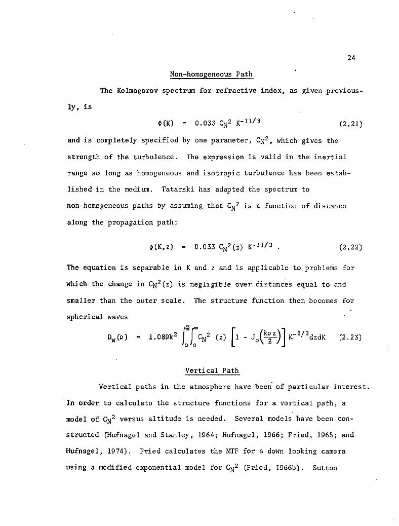
Non-homogeneous Path
The Kolmogorov spectrum for refractive index, as given previous
ly, is
$00 = 0.033 CN2 K-h/3 (2,21)
and is completely specified by one parameter, C 2, which gives the
strength of the turbulence. The expression is valid in the inertial
range so long as homogeneous and isotropic turbulence has been estab
lished in the medium. Tatarski has adapted the spectrum to
non-homogeneous paths by assuming that Cj 2 is a function of distance
along the propagation path:
$(K,z) = 0.033 CN2(Z) K"11/3 . (2.22)
The equation is separable in K and z and is applicable to problems for
which the change in C 2(z) is negligible over distances equal to and
smaller than the outer scale. The structure function then becomes for
spherical waves
Dw(p) = 1.089k2 J J CN2 (z) £L - K"8/3dzdK (2.23)
Vertical Path
Vertical paths in the atmosphere have been of particular interest.
In order to calculate the structure functions for a vertical path, a
model of C 2 versus altitude is needed. Several models have been con
structed (Hufnagel and Stanley, 1964; Hufnagel, 1966; Fried, 1965; and
Hufnagel, 1974). Fried calculates the MTF for a down looking camera
using a modified exponential model for C 2 (Fried, 1966b). Sutton

25
(1969) calculates the up-looking case using the same Cjsj2 model. Farhat
and DeCou (1969) compare up and down looking cases for three CN2 models.
The measurement of C 2 as a function of altitude is a formidable
task. Cj2 vs. altitude has been measured on several balloon flights
(Bufton et al., 1972). Then using pressure and temperature data, Bufton
et al. calculate Cj 2 for a vertical path. It should be mentioned that
these measurements were made at one separation only (p = 1 meter) and
the two-thirds law is assumed for all p.
Application of Wavefront Statistics to Image Quality
Calculated wavefront statistics have been applied to image quality
calculations only for the special case of long time exposures. Knowledge
of the wavefront statistics may in fact be insufficient (analytically)
to determine the statistics of the OTF or psf. It has been shown
(Barakat, 1971), that even if the wavefront perturbations are formed by
a stationary, Gaussian, random process, the OTF statistics can neither
be stationary nor Gaussian. (It is possible to investigate the proper
ties of the OTF using computer generated sample functions based upon the
calculated wavefront statistics and some results using this technique
are presented in Chapter 3).
In the special case of long exposure times, the OTF separates,
and the atmospheric part reduces to simply the ensemble average of the
sheared pupil function. The ATF is consequently a deterministic func
tion.
It has been shown (Strohbehn, 1968), using the central limit
theorem, that it is reasonable to expect the probability density function

26
for the wavefront perturbations, after propagating through a turbulent
medium, to be Gaussian. With only this result, and without the Tatar-
ski theory (or its equivalent) it is possible to make significant state
ments regarding the form of the long exposure time ATF. O'Neill (1963)
gave the ensemble average results assuming that the phase difference
statistics were stationary and Gaussian. This has been extended to
include log-amplitude statistics as well (Shack, 1967); the log-amplitude
and phase-difference are uncorrelated random variables if they are sta
tionary (Shack, 1967):
-a|(l - CA) -a|(l - Cs) (2.24) ATF = e e
a? and a2 are the variances of the log-amplitude and phase-difference, Ju S
and and Cs are the respective autocovariance functions, defined as
follows:
r - P& . r Ps °l = 7T ' Cs = 7T (2.25)
& S
where and ; s are the corresponding autocorrelation functions.
A similar derivation in terms of the structure function takes the
following form (Fried, 1965):
ATF = e"D*/2 e"Ds/2 (2.26)
The structure function form is the most suitable for using the Tatarski
results. When the wavefront statistics are stationary the autocovariance
version of the ATF is equivalent to the structure function version.
Tatarski believes that the structure function is a more general and

27
useful function than the autocovariance function since it is possible
for the structure function to be stationary when the autocovariance
function is not. Fried's derivation of the ATF using the Gaussian
random variable assumption did not invoke stationarity for the
phase-difference statistics but did invoke stationarity for the
log-amplitude.
The Tatarski results for the wave structure function may be sub
stituted into the expression to give the long exposure ATF. In fact,
a study of the propagation of the mutual coherence function through
turbulence (Beran, 1967) has shown that the MCF (which is equal to the
long exposure ATF) is the same as EXP -D/2 when the Tatarski solutions
for D are substituted. The Beran study made no assumption as to the
probability density function, which indicates that this expression for
the ATF is on firm foundation.
When the Tatarski structure functions are substituted into the
ATF expression, some surprising simplifications occur which are not
predicted by the Gaussian random variable (GRV) assumption alone. The
desired result is that the theory permits the calculation of the four
terms which appear in the ATF given by the GRV assumption; that is, the
two variances and the two autocorrelation functions, or at least the
width of the autocorrelation, functions. The surprise is that the
Tatarski results take a much simpler form when put in terms of the wave
structure function. For stationary statistics then, the appropriate
autocorrelation form for the ATF is:

28
-4(i - c„) ATF e
where aw2
(2.27)
C, P£ + Ps
'w
The above appears to be a two parameter expression. The variance indi
cates the level or the strength of the turbulence and the width of the
autocovariance function gives a leveling off point for the ATF. This
feature of the transfer function lends itself to a core-flare interpre
tation in the image plane of psf (Shack, 1968).
Kolonogorov spectrum is assumed, the ATF is reduced still further to a
one parameter expression (the one parameter being Cm2). Fried (1966a)
expresses the five-thirds law in terms of a new parameter, r , which
incorporates CN2 and has found acceptance in the literature:
There can be no core-flare interpretation with this form of the ATF;
i.e., the ATF does not "level off". To a student of optics this simpli
fication might therefore cause some dismay. Nevertheless some good mea
surements over a carefully monitored homogeneous path indicate that the
five-thirds law is valid up to shear distances of about one meter
(Clifford, Bourcius, Ochs, and Ackley, 1971). However, other measure
ments over horizontal paths not so well monitored for homogeneity
Another consequence of the Tatarski result is that when the
ATF (2 .28)

29
(perhaps more representative of typical real paths in the atmosphere)
show structure functions which do level off, sometimes at values which
are significant for the ATF (Bertolotti, Carnevale, Muzii and Sette,
1968, 1974; Gaskill, 1969; Buser, 1971). (See also Chapter 7 of this
report). The question can be raised (but not yet answered) whether
real atmospheric paths are simply inappropriate for the application of
the homogeneous turbulence assumptions or whether the results could be
predicted by suitable modeling of the outer scale over the path. Some
new modeling of the outer scale for vertical paths and the effect on
the ATF is given in Chapter 3.
Reciprocity
Reciprocity is an old concept in the Theory of Electricity and
Magnetism, but seems at first consideration to be contrary to experience
when applied to light propagation in a turbulent medium. By reciprocity
here it is meant that if light from a point source propagates through a
turbulent medium to a point receiver, there will be no change in the
wave amplitude at the receiver if the source and receiver are inter
changed. It is a common experience to note that turbulent cells high
in the atmosphere produce scintillation from star light at a receiver
on the ground, while turbulent cells close to the receiver do not;
scintillation depends upon position along the path. However, further
reflection shows that this common experience is not necessarily a
contradiction to reciprocity. In any event, proof of reciprocity for
Frauenhofer diffraction by a screen is contained in standard texts
(Stone, 1963), as well as for Fresnel diffraction using the Fresnel

30
Kirchhoff diffraction integral (Goodman, 1968; Born and Wolf, 1966).
These proofs are probably sufficient to refute the contradiction since
the turbulent cells can be imagined to be thin enough to be considered
approximately diffraction at a screen.
Recently, the proof of reciprocity has been extended to cover
the case of the receiver and source embedded in a turbulent medium.
It takes four lines to complete the proof using the Huygen-Fresnel
approach (Lutomirski and Yura, 1971b; Shapiro, 1971). The proof has
also been applied to some non-point source transmitter-receiver combi
nations (Fried and Yura, 1972).

CHAPTER 3
MODELING ATMOSPHERIC IMAGE QUALITY
The atmospheric models reported in the literature are based upon
the theoretical studies reviewed in the last chapter. Two extensions to
the existing modeling are presented in this chapter. First, some new
modeling of the outer scale and its effect on long exposure time image
.quality over vertical propagation paths is undertaken. Second, the
theoretical statistics are used to form the basis for one-dimensional
computer generated sample wavefronts; they are used to investigate some
properties of this intermediate exposure time ATF.
Modeling the Outer Scale
The Kolmogorov spectrum of refractive index is valid between the
inner scale and outer scale of turbulence. The power spectrum is pre
sumed to drop to zero at higher frequencies and to level off at lower
frequencies. The inner scale has little effect on image quality, except
for very strongly perturbed wavefronts. The outer scale also has little
effect so long as it is large with respect to the maximum shear values
of interest. (The optical aperture diameter, D0, is the maximum shear
value for the system.) So long as the outer scale is large enough, it
may be considered to be infinite and the five-thirds law valid. Many
workers, including Tatarski, have pointed out the pitfalls involved
when the outer scale is not small.
31

32
The refractive index power spectrum levels off at frequencies
lower than 1/LQ but nothing can be said about the exact form of the
spectrum at these frequencies on the basis of physical theory. It has
been shown (Strohbehn, 1966), however, that the exact form has little
effect on the structure function and that only the point of departure
from the inertial range is significant. Any modified spectrum which
levels off in some way below 1/L0 should give good results. One such
modified specturm (Lutomirski and Yura, 1971b) was given in Chapter 2
and was used to generate the "theoretical" curves shown later in this
report (Chapter 7) for comparison with experimental data. The curves
(Fig. 18, page 145), are consistent with our expectation based upon
Gaussian random variables that the ATF should level off at about the
outer scale. They also show that even if the level-off value of the
ATF is quite low, the slope of the structure function is less than S/3
and consequently the image quality is less degraded than the five-thirds
law would imply.
Curves such as these establish the fact that a variation of the
outer scale could account for the experimental deviations from the
five-thirds law cited in the last chapter although proof would require
a monitored test path with known outer scale variations. Model calcula
tions of the structure function for a variable outer scale can be made by
extending the Tatarski treatment of non-homogeneous paths (Chapter 2) to
include L0 as a function of Z:

33
Dw(P»z) s (.033)8irk2 CN2(z)[l - JQ(Kpz/L)]
EXP[-(M2.| 2]K (3.1)
where L = Total path length and the Lutomirski and Yura modified spectrum
is used.
the question arises as to whether reasonable modeling of the outer scale
could cause a deviation of the structure function from the five-thirds
law over vertical paths. The balloon-borne measurements cited in
Chapter 2 did not include a measurement of the outer scale. Yet, some
measurements on star light (Roddier and Roddier, 1973) do indicate a
deviation from the five-thirds law.
Fried (1967) has used a model for LQ that is monotonically
increasing with altitude h: 0
L 0 = 2 h * t 3 - 2 i
where both LQ and h are in meters. Consortini, Ronchi, and Moroder
(1973) have shown that this model and other similar models do not cause
a deviation from the five-thirds law. However, the spikes in the Cn2
model based upon the balloon measurement cast considerable doubt on the
monotonic Fried L0 model. Figure 1 shows the C 2 derived from one
balloon flight (Flight 6). It seems plausible that the strong fluctua
tions of C 2 might imply strong fluctuations of L0. A region where
Since vertical paths are of the greatest interest in this study

Fig.
Cjj2 VS. ALTITUDE
\
\
BUFTON FLIGHT #6
HUFNAGEL STANLEY
A , 20 SO
ALTITUDE in Km
Cj j2 Profiles.
35
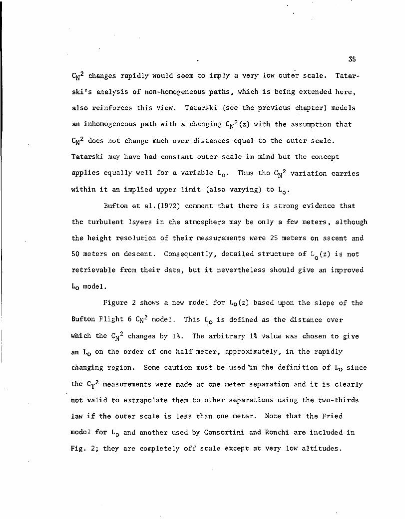
Cjj2 changes rapidly would seem to imply a very low outer scale. Tatar-
ski's analysis of non-homogeneous paths, which is being extended here,
also reinforces this view. Tatarski (see the previous chapter) models
an inhomogeneous path with a changing Cjsj2(z) with the assumption that
C 2 does not change much over distances equal to the outer scale.
Tatarski may have had constant outer scale in mind but the concept
applies equally well for a variable L0. Thus the CN2 variation carries
within it an implied upper limit (also varying) to hQ.
Bufton et al.(1972) comment that there is strong evidence that
the turbulent layers in the atmosphere may be only a few meters, although
the height resolution of their measurements were 25 meters on ascent and
50 meters on descent. Consequently, detailed structure of LQ(z) is not
retrievable from their data, but it nevertheless should give an improved
L0 model.
Figure 2 shows a new model for L0(z) based upon the slope of the
Bufton Flight 6 C^j2 model. This LQ is defined as the distance over
which the C^j2 changes by 1%. The arbitrary 1% value was chosen to give
an L0 on the order of one half meter, approximately, in the rapidly
changing region. Some caution must be used*in the definition of L0 since
the C-p2 measurements were made at one meter separation and it is clearly
not valid to extrapolate them to other separations using the two-thirds
law if the outer scale is less than one meter. Note that the Fried
model for L0 and another used by Consortini and Ronchi are included in
Fig. 2; they are completely off scale except at very low altitudes.

1 METER
Amplitude in Km
Fig. 2. Outer Scale Profile. W o
37
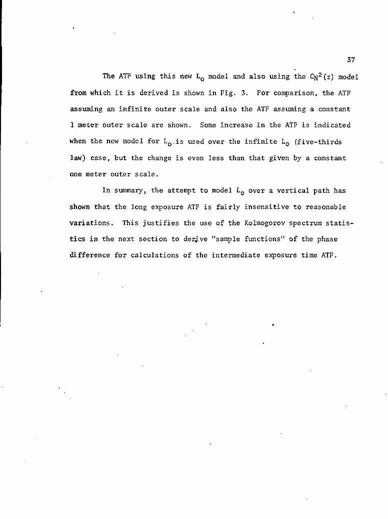
The ATF using this new LQ model and also using the Cn2(z) model
from which it is derived is shown in Fig. 3. For comparison, the ATF
assuming an infinite outer scale and also the ATF assuming a constant
1 meter outer scale are shown. Some increase in the ATF is indicated
when the new model for LQ.is used over the infinite L0 (five-thirds
law) case, but the change is even less than that given by a constant
one meter outer scale.
In summary, the attempt to model L0 over a vertical path has
shown that the long exposure ATF is fairly insensitive to reasonable
variations. This justifies the use of the Kolmogorov spectrum statis
tics in the next section to derive "sample functions" of the phase
difference for calculations of the intermediate exposure time ATF.

38
100
u. u s
L0 = 1 METER
P in Cm
Fig. 3. Long Exposure Time ATF for Various Outer Scale Profiles.

39
Intermediate Exposure Time ATF
The optical transfer function for a system operating in a turbu
lent medium with temporal changes dominated by Taylor's hypothesis
approximately separates into an atmospheric (only) part and an optical
system part for intermediate exposure times. In Appendix I the condition
on exposure time is given
Do T > 3 (3.3)
where
D = Optical aperture diameter
Vj_ = Component of the wind perpendicu
lar to the propagation path.
In addition, the transfer function integrated over one dimension only is
approximately equal to the transfer function integrated over two dimen
sions, under the same exposure time condition (see Appendix I). For an
airborne camera the wind (or pseudo wind) is approximately equal to the
aircraft velocity so that the intermediate exposure time restriction is
quite loose; at a velocity of 200 meters per second the ATF for a 30 cm
diameter camera separates for exposure times longer than 5 msec. Since
this is the most applicable case and since it is one of genuine current
interest, attention in this chapter (as well as Chapters 5 and 6) is
restricted to the airborne camera.
Even for the airborne case intermediate exposure times of
interest are not sufficiently long to encompass an ensemble average of
the wavefront. But instead the ensemble average statistics can be

40
used to generate sample wavefronts which can then be used to calculate
the deterministic ATF. Randomly generated wavefronts have been used
before. Shannon (1971) used a Gaussian probability density function to
generate phase modulated sample functions, over a two dimensional aper
ture. Barakat and Blackman (1973) used the Gaussian probability density
function for phase and amplitude to generate extensive data for a one
dimensional aperture. In both of the above the OTF's (not ATF) were
calculated assuming an aberration free optical system; the "exposure
times" were instantaneous. The attempt made here is to base the sample
functions on the wavefront statistics calculated by Tatarski and applied
to a vertical path for an airborne camera, using non-instantaneous
exposure times.
Sample Wavefronts from the PSD
The PSD (power spectral density) of the log amplitude or phase
of the wavefront is, by the Wiener-Khinchin theorem, the Fourier trans
form of the autocorrelation function R(Ax), for a stationary random
process. Both the PSD and R(Ax) are, of course, ensemble average func
tions. Given the PSD (from Tatarski) we wish to produce a sample func
tion, of necessity a finite sample function, of the random process. This
cannot be done uniquely in any analytical way but a finite record can be
produced which could be from a member of the ensemble.
Consider a finite sample, g(x) from a stationary, ergodic random
process and define a finite sample autocorrelation function as follows:

41
x+T/2
RpfAx; x) = g(x)g(x + Ax)dx (3.4)
x-T/2
Define the finite sample PSD as the Fourier transform of R^fAx, x). By
the ergodic theorem [see Papoulis (1965, Chapter 9) for conditions.]
RTCAX» X) = R(AX> C3-5^
Alternately, the average of a large number of such functions, RT(Ax,x),
approaches the ensemble average function R(Ax). Similarly, the average
of a large number of finite sample PSDs (defined as above) approaches
the ensemble average PSD (easily proved by interchanging the order of
integration). An alternate route from this sample wavefront to the PSD,
or to the finite sample PSD, follows from the convolution theorem; the
PSD is the modulus square of the Fourier transform of the sample function.
The process is not reversible, given a finite sample PSD, we
cannot uniquely find the finite sample function which produced it. How
ever, a possible sample function may be produced as follows. The square
root of the finite sample PSD gives the modulus of the Fourier transform
of the sample function. Using computer generated random numbers, a ran
dom phase is added to modulus and the inverse Fourier transform results
in a possible finite length sample function.
The finite sample PSD is produced from the ensemble average PSD
as follows. A random spectrum is generated by the computer over the
frequencies of interest. This is multiplied by the ensemble average PSD.

42
The result is considered to be the finite sample PSD; it meets the test
that the average of a large number of finite sample PSDs generated in
this manner will converge toward the ensemble average PSD.
Vertical Path Temporal Statistics
Using Taylor's hypothesis the spatial statistics [the PSD and
R(Ax)] may be converted to temporal statistics. Temporal statistics are
useful for the model ATF calculations since they compare directly with
the ATF measurements described in Chapter 5: a dual purpose is served
in these calculations in that they provide a test of the data reduction
methods for the ATF measurement technique.
Clifford (1971) has derived the temporal power spectrum of the
phase, phase difference and amplitude for a spherical wave in a turbulent
(homogeneous) frozen atmosphere:
PSD. .033 5, sin0^-) a, /Q << 1
k2L C„2v 3 [1 ; 066 N (^o In » l
psd* L .245
81
<a2> 1 + .1190
f -8/q o n 3
ffl « l
la » l
(3.6)
with the restrictions

43
ig *o « (XL)"2 « Lq
fo < v/L0
where f = temporal frequency (Hz)
v = perpendicular component of wind velocity
L total path length
<A2>
fo
0.124 k7/6 L11/6 CN2
f/f0
v/ (2/irXL)^
These spectra apply to a homogeneous path with camera and object fixed
and with a constant velocity wind. However, the application for this
section is, instead, a moving camera with an inhomogeneous path. It
may be possible to incorporate the proper geometry, perhaps even using
We are satisfied here with a first approximation to this, however. That
is, the PSDs are assumed here to have the same functional form given by
Clifford (above) and the constants (L %2) and (L7/3C 2) for phase and
amplitude respectively are adjusted to match (approximately) integrated
values based on the Bufton Flight 6 data.
the Cjyj2(Z) variations (Bufton Flight 6) used in the preceding section.
In the phase PSD the following approximation is made:
h max
(3.7)
where the value chosen is equal to the indicated integral for Flight 6
as reported by Bufton (1973). In the log amplitude PSD the substitution
t
44
h 11/ ,• t max 5. _
V L 6 * TT I CN2 L 6 dh = .65 x 10"9 m (3.8)
h0
where again an integrated value reported by Bufton was used. At best,
these approximations give a crude estimate of the vertical propagation
path and conclusions made must be considered with some reservations.
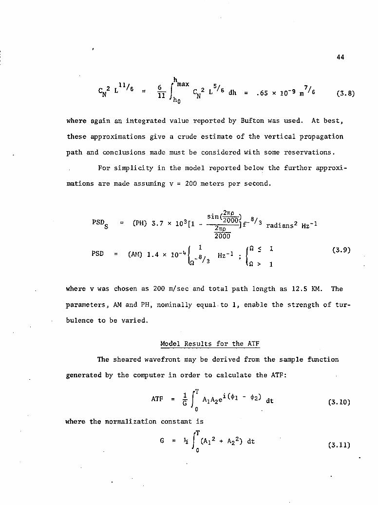
For simplicity in the model reported below the further approxi
mations are made assuming v = 200 meters per second.
. ,2up .
»s = (PH) 3.7 x i03[i . ln™00]f-81* radians2 Hz"1
PSD = (AM) 1.4 x 10-{ J / 3 Hz"1 ; J
2TTP 2000
< 1 (3.9)
a > 1
where v was chosen as 200 m/sec and total path length as 12.5 KM. The
parameters, AM and PH, nominally equal to 1, enable the strength of tur
bulence to be varied.
Model Results for the ATF
The sheared wavefront may be derived from the sample function
generated by the computer in order to calculate the ATF:
rji
ATF " k J AlA2ait+1 " « dt (3.10) 0
where the normalization constant is
fT G = h j (A22 + A22) dt (3.11)

45
The sample function for the phase difference gives directly and
the sample function for log amplitude gives log Aj. A2 is formed from
Aj as follows
Aa(t) = Aj(t + —) v (3.12)
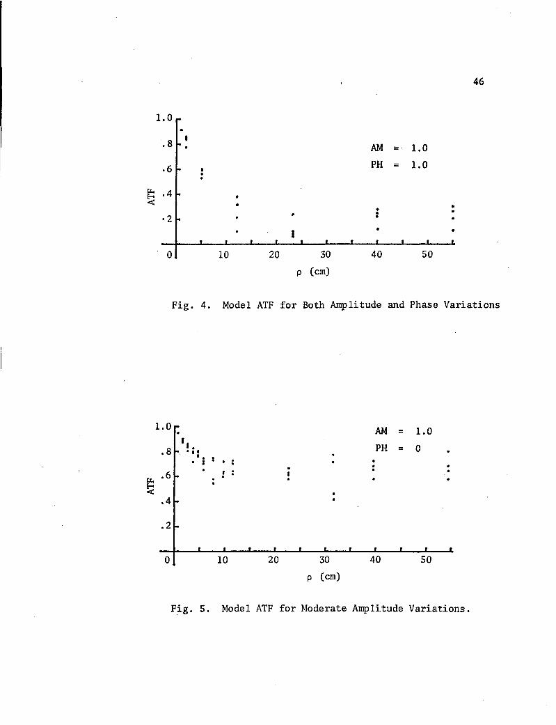
The ATF calculated for 12.8 msec exposure times is shown in Fig.
4. A sample sheared wavefront was generated for 52 msec period and
broken down into 4 segments for the ATF calculation. Thus four transfer
factors are shown for each value of p chosen. A new wavefront was
generated for each p; this seems inconvenient for visualizing the entire
ATF(p) curve but corresponds to the method of measurement of the ATF
described in Chapter 5.
Comparison of Fig. 4 with the long time exposure curve gener
ated from the Flight #6 data shown in Fig. 3, page 38, gives some indi
cation of the errors made in the approximations used to generate the
intermediate time exposure model. The two figures agree reasonably well.
The ATF in the case of amplitude only wavefront variations is
shown in Fig. 5. Note that the phase effect is dominant at large fre
quencies but the effect of amplitude at lower frequencies is approxi
mately equal. This observation is consistent with the Tatarski
solutions. Figure 6 shows again amplitude only but for a reduced
strength of turbulence. Note that the correlation length is approximately
unchanged but the level-off value is much higher.
The variation of ATF with exposure time is shown in Fig. 7 for
a 12 cm shear value. Note that the long time exposure, 50 msec, value
46
1 . 0
. 8
.6
A Sc '4
AM = 1.0
PH = 1.0
I .1 I ' » » I I I I L 10 20 30 40 50
P (cm)
Fig. 4. Model ATF for Both Amplitude and Phase Variations
I. ' • ! • 3 • • 3 •
i :
AM = 1.0
PH = 0
10 20 30
P (cm)
40 50
Fig. 5. Model ATF for Moderate Amplitude Variations.

47
1 . 0
. 8
. 6 £L| H < .4
* » ;
.1 ' ' ' ' ' ' I t I L
10 20 30
P Ccm)
40 50
Fig. 6. Model ATF for Small Amplitude Variations.
1 .Or
. 8 .
.6 -
.4.
. 2 *
10 20 30 40
T (msec)
50
Fig. 7. Variation of Model Transfer Factors with Exposure Time.

48
is 19% while all of the values for time exposures 6 msec and less are
higher than that value.
The effect of strength of turbulence (amplitude and phase) on
the 5 cm shear transfer factor is shown in Fig. 8. The "nominal" value
of one for both AM and PH is based upon the Bufton Flight 6 integrals
as described above. The resulting ATF values are very sensitive to
AM and PH near the nominal value. This indicates that an experimental
measurement program might be expected to see large changes in ATF for
reasonable hour-to-hour variations in turbulence.

49
P T AM
.5 1 . 0
5 cm 64 msec PH
AM, PH
Fig. 8. Model ATF vs. Turbulent Strength Parameters.
CHAPTER 4
MEASUREMENT OF IMAGE QUALITY: REVIEW AND GENERAL CONSIDERATIONS
The optical testing literature is far too extensive for review
here. However, those features of the theory of testing which permit
evaluation of the reported atmospheric measurements will be given; they
also establish a groundwork for discussing new techniques.
Measurements of image quality may be made on any of the basic
functions of image formation theory: the pupil function, the sheared
pupil function, the optical transfer function, or the point spread func
tion. They were discussed in Chapter 1 with respect to time varying
wavefronts; the time varying nature of the wavefront is the source of
the increased difficulty of atmospheric image quality evaluation as
compared to that in the normal testing laboratory. However, the best
way to classify testing techniques is not necessairly through the func
tions of image formation theory. The measurements in optical testing
are made with square law detectors which are not sensitive to phase
information. Thus, it is not possible to measure the pupil function
directly since the phase of the pupil function is the most important
ingredient.
The most natural classification system is one which follows the
techniques by which, the phase of the wavefront is retained. Measurements
may be made directly on the intensity distribution of the point spread
50

51
function. The psf is always real and positive but the effects of the
wavefront phase are included in it. Geometric tests (ray optics) such
as the Foucault test, the wire test, and the Hartmann test are used to
measure the slope of the wavefront in the pupil and hence the phase may
be retrieved from them. Interference tests can measure the pupil func
tion indirectly, by measuring the intensity of the pupil function plus a
reference wave. Certain choices of the reference wave give a direct
measurement of the sheared pupil function or of the optical transfer
function.
A brief discussion of each technique is given below from the
standpoint of atmospheric testing.
Point Spread Function Measurement
The measurement of the point spread function (psf) of necessity
includes the optical system effects as well as the atmospheric effects.
Isolating the effect of the atmosphere can be a major drawback. There
is no general way to get the pupil function form the psf so that these
results apply only to the particular optical system used and can only
obliquely be used to determine the image quality for another optical
system. If, for example, conditions for separation of the transfer
function apply, then part of the ATF can be determined from the psf by
Fourier transforming (to get the OTF) and factoring out the known optical
system OTF.
The routine measurement of the point spread function diameter
at astronomical sites has been described (J. Stock and G. Keller, 1960).
It has important application in the selection of future astronomical
52
sites (Meinel, 1960). For this application a star is used as a point
source object. A technique for continuously monitoring the short term
blur and the image motion of star images on a small telescope has been
devised (Ramsay and Kobler, 1962). By use of a rotating chopper in the
image plane, the results were interpreted directly, in terms of the
modulus of the transfer function at the spatial frequency determined by
the sector size of the chopper. Coulman (1965, 1966) has used the same
technique for studying propagation over horizontal paths. Notable recent
results for stellar sources have been reported (Bufton and Genatt, 1971).
The short term blur, or rather, the short term MTF for one spatial fre
quency is continuously generated by this technique and the image motion
was used by Bufton and Genatt to convert this to a long term MTF.
Geometrical Measurement
Geometrical measurements play a vital role in image quality
measurement in an optical testing laboratory. They are used to measure
the ray directions in the exit pupil and hence give the slope of the
wavefront from which the pupil function can be acquired by integration.
The quantitative geometrical techniques such as the wire test,
require time to perform and probably have found little use for the study
of time varying wavefronts. As exception is the Hartmann test (Golden,
i975). Although the classical Hartmann test is not suitable for time
varying wavefronts, Golden has developed a new dynamic Hartmann test
capable of extreme accuracy. Consortini (1974) has used the basic
concepts involved in the Hartmann test on turbulent wavefronts but in
a less general way than the Hartmann test itself.

53
Interference Techniques
Interference techniques are often used in optical testing to
provide a measure of the pupil function. In atmospheric measurements
they have more often been used to obtain a direct measure of the sheared
pupil function, or of the OTF. The primary difference in these tech
niques is in the nature of the reference wavefront which is produced.
Four different reference wave techniques are discussed below.
A reference wavefront added to the wavefront in the pupil plane
produces an irradiance (or a signal using a square law detector) that is
proportional to
A(x,y)e1*tx'5'' * A (4.1)
= A (x,y) + Ar (x,y) + 2A(x,y) Ar(x,y) cos [<j>(x,y) - <j>r(x,y)]
where the subscript r denotes the reference wave.
Note that the phase, 4>, is not thrown away but is contained in
argument of the cosine function. Also note that it is the phase differ
ence (<|> -<J>r) which appears even though the wavefronts were summed (before
detection). With random wavefronts one of the problems is extracting
the desired phase information from the total signal expressed above.
In contrast, this is usually a trivial problem with deterministic optical
testing (because A(x,y) and Ar(x,y) are constants) and is rarely even
mentioned there.
In testing with no time varying wavefront, a spherical reference
wave with center of curvature at the image point is very useful. Then

54
the phase difference (0 -0r) is proportional to the definition of the
aberration function, W; the intensity distribution of the resulting
interferogram is
Ai2 + A22 + 2A1A2 cos 2ir W (4.2)
or, if Ai and A 2 are equal and constant, the intensity if proportional
(1 + cos 2I TW) . (4.3)
The extraction of W from this expression is usually accomplished, not by
measuring intensity, but with a trick, which is extremely useful in
atmospheric testing as well. The reference wavefront is tilted with
respect to the test wavefront so that the intensity distribution is pro
portional to
[1 + cos 2TT (lV(x,y) + X sin0)] (4.4)
where 0 is the tilt angle between wavefront. With no aberration, the
interferogram would consist of straight line fringes; with aberration,
W is spatially heterodyned onto the tile angle spatial frequency. W is
extracted by measuring the deviation of the fringes from a straight line.
An early interference experiment on atmospheric propagation fits, or
almost fits, into this category (Herrick and Meyer-Arendt, 1966). The
experiment used a Michelson interferometer with one long arm over a
several kilometer atmospheric path, and one arm, an unperturbed reference
(short), path. Fringe patterns were recorded but only casual observa
tions about them (no data reduction) are reported. The experiment was
not performed with a point source so that a direct measure of MTF could
not be accomplished, but the biggest problem in reducing data from such

55
ail experiment is that there is so much data. Some simplification of the
full data over a practical exposure time is a necessity.
An excellent experiment using a Michelson interferometer (Bour-
cius and Clifford, 1970) was conducted over a short (50 meter) homogen
eous path in such a way that significant data was collected. The
simplification they made was to sample the interferogram at one point
of the wavefront only. Using four photodetectors, they recorded simul
taneously as a function of time
1) A2 + Ar2 + 2A A^ cos(<f> - 4>r)
2) A2 + Ar2 + 2A Ar sin ($ - $ )
3) A2
4) A 2 J r
The photodetector outputs were used to isolate cos (<j> -<{>r) and the
sin(<j> -<{>r) . With both the sine and cosine it is possible to extract
C<f> - without ambiguities. <j>r is an arbitrary constant, so that
Bourcius and Clifford have a record of <#>([t) for one point in space.
Of course, this is not enough to determine the transfer function, but
by applying the Taylor "frozen atmosphere" hypothesis they derived
A<|>(x) by setting x = vt, where v = wind velocity perpendicular to the
path. (Subsequent measurements (Clifford et al., 1971) have verified
the applicability of Taylor's hypothesis.) Bourcius and Clifford use
the data to calculate the phase structure function for a plane parallel
wave. Since this is not the same as the phase structure function for
56
a spherical (point source) wave, the transfer function cannot be given
from it directly, although the conversion, for homogeneous turbulence,
is straightforward.
In the second interferometer type, the reference signal is
sheared version of the wavefront itself. In this, a shearing inter
ferometer, the intensity interferogram is proportional to
Al2 + a22 + 2Acos[<j>(x,y) - <f>(x + Ax,y)] (4.5)
In deterministic optical testing, shearing interferometers have found
great use in the indirect measurement of the pupil function. The sheared
phase difference is extracted easily, since Aj and A2 are constant (in
the testing laboratory). The expression above implies that the two wave-
fronts are sheared (i.e., laterally displaced) such that the center of
curvature remains common to both; if the centers of curvature are dis
placed from one another, the phase difference is spatially heterodyned
onto a series of straight line fringes. The sheared phase difference
is extracted easily, since in the lab A^ and A2 are constant and the
contribution of various optical aberrations to the interference pattern
are well known.
It is not so easy to solve for the phase when the perturbations
are due to a random process such as the atmosphere instead of well known
symmetrical aberrations. The intensity distribution of the shearing
pattern contains within it the real part of the optical transfer factor

57
for one shear value. Integrating the intensity gives this factor if
the Ai2 + A22 terms and the heterodyning term can be removed from it.
A shearing interferometer for use in the exit pupil of an optical
system used in the atmosphere has been reported (Kelsall, 1973). This
is a very stable cube-corner instrument whose measurements include the
effect of the optical system with which it is used. The intensity distri
bution is integrated over the entire overlap region. The effect of
Ai2 + A22 is thought to be eliminated by modulating the optical path in
one arm, but at a fairly low frequency (60 Hz). By considering only
the amplitude of the modulated signal, the instantaneous MTF as a func
tion of time is measured. The phase of the modulated signal, which is
equal to the phase of the instantaneous OTF, is discarded by Kelsall, a
distinct disadvantage except for systems which track the instantaneous
average tilt of the wavefront. Otherwise, the intermediate exposure
time OTF is lost. The phase could be recovered, however, if desired,
but this would probably require more careful attention given to the
errors introduced by the effect of Ai2 + A22 and A A in the presence
of scintillation, especially for airborne systems with a large
psuedo-wind.
Other exit pupil shearing interferometers have been reported
for use with time varying wavefronts. One uses a grating shearing
interferometer (Burlamacchi, Consortini, and Ronchi, 1967) and one
applied with stellar targets using a Michelson interferometer (Roddier
and Roddier, 1973). The Michelson interferometer has two outputs which
are 180° out of phase. Roddier and Roddier eliminate A 2 + A22 by

58
simply subtracting the two outputs; this is clearly more elegant and
more error free than separating A}2 + A22 in frequency space from a
single output. The shear in this instrument is accomplished with a tilt
of the mirror in one arm about the on axis image point. Thus for an on
axis point the shear is purely lateral (both wavefronts retain the same
center of curvature). However, for off axis points, the centers diverge
slightly, which has the primary effect of only adding a constant to the
optical path of one arm. The constant is of course a function of field
angle so that a star which traverses the field of view gives a modulated
output. Roddier and Roddier use the visibility of this output to indi
cate the long term MTF, which appears to be valid for a telescope which
tracks the star at a uniform rate.
Shearing interferometers have also been used in the entrance
pupil, enabling measurements on the atmosphere alone. Experiments using
Mach-Zender interferometers have been performed (Buser and Born, 1970;
Buser, 1971; Bertolotti, Carnevale, Crosignani and P. Di Porto, 1969).
which closely resemble shearing of the entrance pupil. For a true shear
ing interferometer a single point source should be used. Nevertheless,
the results of Buser and Born are particularly interesting with respect
to the effect of A 2 and A22 on their (spatially heterodyned) fringes.
A single source (if not a single point source) has been used in
a single and a "multibeam" shearing interferometer (Bertolotti, Carnevale,
Muzzi, and Sette, 1968, 1970). The sheared signal for two points in the
aperture was recorded (single beam) and for two points in the aperture
was recorded (single beam) and for two points with several different

59
separations simultaneously (multibeam). A shearing interferometer experi
ment over a carefully controlled 50 meter horizontal path, sampling the
wavefront at four different separations (sequentially) have been reported
(Clifford, Bourcius, Ochs and Ackley, 1971).
Another experiment for accessing the effect of the atmosphere on
holographic images (Gaskill, 1969) is important conceptually, here, since
it can be interpreted as a shearing interferometer experiment by invoking
the reciprocity of the atmosphere. Gaskill used a point source reference
beam and a point source target to measure the impulse response through
the atmosphere of a lensless Fourier transform hologram. The two coher
ent point sources were projected through the atmosphere, forming an inter
ference pattern (Young's fringes) on a photographic plate (hologram).
The intensity at a single point in the interference pattern is identical
to the intensity of a shearing interferometer output which employed a
single point source at that position and sampled the wavefront at the
two points at which Gaskill's point sources were placed.
Two other interferometer types have been suggested for use in
atmospheric measurements, but they are exit pupil instruments. A fold
ing or reversing wavefront interferometer (Shack, 1966) and an inverting
wavefront interferometer (Breckinridge, 1975). The distribution of
intensity in the interferogram for those contains within it the change
in the OTF with spatial frequency. However, the Aj2 + A22 term can
probably be extracted only in the long term average (in which case it
is constant across the interferogram) and hence these interferometers
may not be useful for intermediate exposure times.

60
New Techniques
The object of this section is to show how the general considera
tions discussed so far lead to specific proposals for new, improved mea
surements of the atmosphere's affect on image quality. To some extent
"new techniques" is a misnomer since what is really covered is a synthesis
of old techniques with new twists.
The desired result is a technique for measuring the atmosphere
alone which can then be applied to any optical system. The obvious
tendency is then to overlook psf measurements and exit pupil measurements
in favor of entrance pupil measurements. Also, for versatility, a
one-way propagation technique is desired; that is, a Michelson inter
ferometer, with two-way propagation over a test atmospheric path in one
arm, is too cumbersome. Any interference technique using a spherical
reference wave is, equally, undesirable. This leaves a shearing inter
ferometer as the most likely choice.
The amount of data required for completely specifying image
quality is so great as to preclude a simple measurement technique.
However, there is an important class of applications in which it is
sufficient to specify the atmospheric effects at two points only in the
entrance pupil (as a function of time). This simplification rests
mainly on the application of Taylor's frozen atmosphere hypothesis as
described in the introduction. Another fallout from using Taylor's
hypothesis is that in many circumstances, the transfer function (as well
as the pupil function) separates into an atmospheric part (the ATF) and
an optical system part. This may further simplify the data reduction.

61
The shearing interferometer output for two points in the aper
ture as a function of time is given by:
S(t) = Ai2(t) + A22(t) + 2A1(t)A2(t) cos (A<fr12(t))
To specify the image quality the output must be reduced to yield the
pupil function:
ACtJe1"1' (4.7)
or the sheared pupil function:
Ai(t)A2(t)el(A<h2Ct)3 (4,8)
or the transfer function:
T | J A1Ct)A2Ct)eiCA,J>l2(t)) dt (4.9)
The most remarkable feature of the two point shearing interferometer out
put is the ease with which the ATF can be extracted. To facilitate sep
aration of the Ai2 + A22 term the optical path in one interferometer arm
may be modulated. Then taking the finite Fourier transform of the data
record gives a result which explicitly includes the ATF. Such an ATF
experiment is covered in detail in Chapter 5. The particular application
chosen for Chapter 5 is the measurement of the ATF for a down-looking,
airborne camera, since Taylor's hypothesis holds for almost all exposure
times of interest in that case. In addition, the reciprocity of the

62
atmosphere is used to simplify the implementation of the experiment.
Instead of using a point source on the ground, propagating to a shearing
interferometer on the aircraft, a point source on the aircraft is
sheared to give two coherent points in the entrance pupil which propa
gate to a point receiver on the ground.
The AJ + A2 term may BE more reliably rejected if two outputs
with opposite phase are available:
SjCt) = AJ2(t) + A22(t) + 2AJA2COS ((A^GCT))
(4.10) S2(t) = A!2(t) + A22(t) - 2AJA2COS CCA«f>12 C"T) 3
Then the real part of the sheared pupil function may be obtained by
simply subtracting the two outputs. This could be done with the same
experimental plan used in Chapter 5 if the two point sources are set
at orthogonal circular polarizations and the receiver uses a beamsplitter
and two photodetectors, each with a linear analyzer (orthogonal to one
another).
Although it is not explicitly mentioned, all the necessary con
siderations for performing such a sheared pupil function experiment are
included in Chapter 6. However, Chapter 6 goes one step further. Not
only is the sheared pupil function obtained but also, with two additional
photodetector channels (a total of 4 channels) the quadrature term is
obtained:
AjA2 sin(A<j>12(t)) C4.ll)

63
Using these two terms the phase difference Aipiz and A1A2 may be isolated.
Gruenzel (1972) has described a technique for converting the one dimen
sional phase difference obtained from the Chapter 6 measurement into
the phase <j>. A similar technique may be used for obtaining A from
AiA2 (Philbrick, 1975), if desired. Thus the Chapter 6 measurement is
a pupil function experiment, using the same experimental plan as the ATF
experiment of Chapter 5.

CHAPTER 5
APPLICATION OF THE TWO POINT SOURCE TECHNIQUE TO THE MEASUREMENT OF THE TRANSFER FUNCTION
The measurement of the transfer function for a specific applica
tion, the case of a down-looking airborne camera, is presented in this
chapter. A description of the experiment, the system design, and an
analysis of the data reduction and of the error sources are given. An
experiment for a moving "camera" as discussed here is quite different
from an experiment for measuring the transfer function over a fixed path,
especially in the system design and in the error analysis. Since the
equipment built for the vertical path was tested over a horizontal fixed
path (see Chapter 7) some comments and description of a fixed path experi
ment are included here when appropriate. Also, an effort is made to
point out those areas where a different design or technique would be
significantly better for a fixed path experiment.
The moving camera has been the one of greatest interest in this
study for two reasons. One, the instrumentation problems involved in
measuring the transfer function of a moving camera are so difficult as
to accentuate the advantage of a simple technique such as the two point
source technique; and, two, the application of the frozen atmosphere
hypothesis and the simplification which it brings to the two point source
transfer function measurement are much more extensive for a moving cam
era since the atmospheric hypothesis is valid for a much wider range of
exposure times.)
64

65
Experiment Descriptions
A brief description of three experiments for measuring the trans
fer function are given below. The first, the airborne experiment, is the
primary topic of interest since the remainder of this chapter is tailored
to this experiment. In the second, a fixed path experiment with a rotat
ing transmitter is described to emphasize the similarity to the airborne
experiment. The third is a fixed path, non-rotating transmitter; it is
a superior technique for the fixed path measurement but one which has
not been developed in this study.
Airborne Experiment
The measurement of the airborne camera transfer function is well
suited to the two point source technique. The two point source trans
mitter is carried on the aircraft in the same position as the camera
itself. The two beams are projected from the aircraft to the ground
where they overlap, producing Young's fringes, approximately straight
line fringes, perpendicular to the axis of the aircraft. Simple
photo-detector receivers are placed on the ground for detecting the
fringes as the aircraft passes overhead. The output of a receiver is
proportional to
SCt) = Ax2 • A22 * 2A1A2cos(2Mt • ^
where the heterodyne frequency, to is produced by the fringes being swept
past. The output is recorded on tape for data reduction later and also
may be fed immediately to a mini-computer for on-line assessment of the
data.

66
The simplicity of the ground receivers impart a certain flexi
bility to the experiment. The number of receivers which may be used is
unlimited (except by practical cost considerations). A number of
receivers may be spread out perpendicular to the aircraft path to insure
data acquisition and relieve any uncertainty in exact aircraft position
or orientation. The receivers may be bunched fairly close together for
measuring the extent of an aplanatic zone. Or, the receivers may be
strung out along the flight path to multiply the data obtained from a
single pass.
The data reduction is accomplished by a simple Fourier transform
operation with a mini-computer by which the heterodyned interference
term is separated from the normalization term and both are integrated.
The ratio of the two integrals is the Atmospheric Transfer Factor for
the particular source separation (i.e.,spatial frequency) used. The
same data may be used for several different exposure times. The point
source separation may be set for each pass of the aircraft so that the
transfer function may be built up on successive passes. (This is not
a basic limitation of the technique since multiple point sources could
be used to get several transfer factors simultaneously.)
Fixed Path, Rotating Transmitter Experiment
This experiment is conducted like the aircraft experiment except
that the fringe pattern is rotated past the receiver to provide the
heterodyne frequency. The transmitter may be more carefully aimed and
the beam characteristic may be examined visually at the receiver site
when stationary. Only one receiver is required.

67
The major difference in these two experiments is in the atmo
sphere itself. The horizontal path measurement is more likely to contain
strong turbulence. The change with time of the atmospheric ensembles is
independent of the transmitter rotation (this is not true of course for
the airborne experiment).
This experiment simulates the airborne experiment very well in
that the beam divergence, the signal-to-noise ratio, and some of the
error sources are the same or similar.
Fixed Path, Fixed Transmitter Experiment
For a fixed path system it is better to use an active phase
varying device in one beam of the transmitter than to use mechanical
rotation. In this way a much higher heterodyne frequency can be
achieved which enables separation of the interference term to be accom
plished with greater accuracy. Also, the beam angle may be made much
narrower which enables the experiment to be performed with a relatively
low power laser. A Pockel's cell can easily be used to provide the
modulation, although in this case the effect is not a linear one as is
the translating case. A sinusoidally varying Pockel's cell is discussed
in the section on the heterodyne term.
System Design
Transmitter
The transmitter shown in Fig. 9 is a versatile design which
permits quick change of point source separation, Ax, and beam diameter.
The laser is a one watt argon laser (Spectra Physics Model 164) with

Laser
Beamsplitter
I / I
Transmitter
Zoom
-V
•
-/
Beam Expander
•>
Spectral Filter Slit Obi ective
Field Stop
Detector and 1 Preamp Field Lens
Amplifier Batteries
Receiver
Fig. 9. System Design.

69
Litrow prism for selecting the 5145 A line and an etalon for extending
the coherence length. The Jodon beam expander uses a well corrected
microscope objective; its primary purpose is to expand the beam to a
sufficient size so that dust particles on subsequent optics cannot
scatter a significant amount of energy. The zoom lens with the follow
ing doublet act as a second beam expander which can be varied with the
zoom setting to control the beam diameter at the receiver. A pinhole
may be placed at the common focus of these two lenses. The beamsplitter
is a front surface dielectric coated flat (Priel 2-inch precision flat)
with a 50-50 split for TE incident wave. A compensator plate is used in
the reflected beam. The final two mirrors are mounted on precision rails
and geared with a rach and pinion to a Geneva drive. The Geneva can
change the separation in five centimeter increments from 20 to 55 centi
meters. The final converging lenses move with the mirrors. One setting
of the Geneva is such that each beam is intercepted by a pair of mirrors
which adjust the separation to 5 centimeters. This is the narrowest
separation available with this configuration.
Note that the only focusing elements following the beamsplitter
are the final lenses and these are well matched (A/10) plano-convex
lenses fabricated and tested in the Optical Sciences Center Optical Shop.
All the plane mirrors used were polished in the Optical Sciences Center
Optical Shop (A/10) and coated in the Optical Sciences Center Thin Film
Laboratory.

70
This transmitter was specifically designed for a translating
operation (airborne) but it has been mounted on a rotating table with
variable speed drive (1 to 6 rpm) for stationary path measurement.
Receiver
The receiver also shown in Fig. 9, page 71, has a simple radiom
eter design. The slit (selected to be approximately 1/4 of the fringe
period) in front of the objective lens is the entrance pupil. A one O
inch interference filter limits the spectral bandwidths to 70 A (a Dit-
ric 3-cavity filter). The field stop determines the field of view and
can be changed to accommodate background level. The field lens images
the entrance pupil onto a .1-inch diameter silicon photodiode (EGG
SD-100). The preamplifier and amplifier were designed at the Optical
Sciences Center to feed the signal onto an analog tape recorder at up
to 60 ips. The signal is then fed to an A/D converter and to a
MOD-Comp. Minicomputer for processing.
Signal-to-noise Ratio
The signal-to-noise ratio is subject to several uncertainties
during the experiment; examples are the variation of laser output power,
the effect of large intensity scintillations, the variation of atmo
spheric attenuation (aerosol scattering), and noise level changes, etc.
However, the signal level can be easily controlled with relatively little
effect on the amount of acquired data. This gives flexibility in adjust
ing the uncertainties and, ideally, in adjusting the goals of the experi
ment as well. The extension of the experiment to include multichannel

71
pupil function measurement (as discussed in the following chapter) is
an example of the latter. The signal-to-noise ratio is established here
with desirable but arbitrary beam characteristics; frcm one to two orders
of magnitude increase in signal could be achieved if required.
The signal-to-noise (voltage) ratio for a bright fringe at the
receiver is given as follows:
-d 5 /M 2 PLTAWR S/N " (ir/4)Bz NEP/Af (5-2)
where P. = Laser output power L
T , T , T = Transmission of the atmosphere, the transmitter, a t r
and receiver respectively.
= Collecting area of the receiver
r = Distance of the receiver from the center of the beam.
B = Beam diameter (to 1/e power points)
NEP = System Noise equivalent power referenced to 1 Hz. band
width.
Af = Bandwidth
The factor of 2 results from the bright fringe specification.

72
The effective rms noise for the system is the root sum square
of several statistically independent noise sources:
NEP SEf = [nd2 + nb2 + nt2 + na2]1/2 C5*3)
where n^ = detector noise
njj - background noise
n . = thermal or Johnson noise
na = amplifier noise
The noise from each source depends upon the bandwidth of the
receiver; the data reductions system vised is in effect a very narrow
band filter (since only two points of the Fourier transform are used)
but since the simplest triggering technique uses the entire bandwidth,
the full 20KHZ is used for signal-to-noise ratio calculations. Each
calculated noise level is given in Table 1 with pertinent parameters
used in the calculations.
The detector noise can be calculated from the
by the manufacturer:
(5.4)
n /AdAf d D*
where D* = 10*2 watt"* cm Hz*''2
2 Aj = Detector Area (.05cm )

73
The thermal noise shown in Table 1 assumes that a 10 megohm
feedback resistor, Rj is the noise source:
nt = I /kTAf/Rf (5.5)
where k = Boltzman's constant
T = Temperature in °K
R = Responsivity of the detector in amps per watt.
Table 1. Noise Parameters.
3x10 watts
nb 1x10 watts
AA
VR
2X10"1* watts
10 watts
"t
%
D* 1012 watts -1 cm Hz1 2
Af 20 KHz
2 A, .05 cm
-1 R .12 amps watt
-3 -2 -1 -1 Nb 10 watts cm steradian micron
-3 . 5x10 microns
2 A_ 1 cm (minimum)
n
T 300° K
.01 steradian

74
The amplifier noise is an estimate. The background noise is a
shot noise induced by radiation from the sky background. The rms shot
noise (Oliver, 1965) referenced to the input power is
nb = ^ /2eIAf (5.6)
where e = Electron charge
I = D.C. current generated by the background radiation
The current I depends upon the background radiance Ng and the solid
angle field of view, f2:
I = NbS5AXArRTr (5.7)
where AX = spectral bandwidth.
The estimate of the background spectral radiance is based on a curve in
the Military Infrared Handbook (Wolfe, 1965).
The parameters used to calculate the signal level are given in
Table 2. The atmospheric transmission factor is assumed to be a nominal
value for the ever present water aerosol.
Tj is primarily the result of many surface reflections, while
TR is dominated by the losses in the spectral filter. With receivers
spaced at 50-meter intervals, the value of r ''and B are such to insure r max
approximately one-half second of useful data for any path across the
receiver line.
The light hitting the detector, given the values of Table 1,
page 73, is 6x10"9 watts. This implies a signal-to-noise ratio of
approximately 30.

75
Table 2. Signal Level Parameters
P L
1.2 watt
T A 85
T, T
.50
T, R
40
B 100 meters
r max 50 meters
Heterodyne Term
A key part of the two point source measurement is that the inter
ference term is heterodyned to a high frequency which enables it to be
separated from the normalization term. There are some slight differences
in the development of this term for the rotating transmitter as compared
to the translating one. Both lead to a linear phase term in the first
approximation. The deviations from the linear phase is evaluated later
in the section on error sources (non-straight line fringes) and shown
there to introduce a negligible error. The phase term due to a Pockel's
cell modulation in one arm of the transmitter is not linear and differs
so much from the translating transmitter that a brief discussion of this
case is given here.
Rotating Transmitter
The geometry for the rotating transmitter is shown in Fig. 10.
The rotation is assumed to pivot about a point midway between the two
point sources with a constant angular velocity, 0. In the figure the

Point Source Point £ Source
Point Source
Point Receiver
Point Receiver
Point Source^
(a)
Rotating Transmitter
(b)
Translating Transmitter
Fig. 10. Heterodyne Term Geometry

77
transmitter is shown rotated at an angle 0 which is assumed to be a
small angle, (i.e., the transmitted beams are on the order of one degree
in angular subtense). The wave amplitudes at the point receiver from
each source are
V, - t5.8)
where A is the modulus of the wave, Ri and R2 are the optical path lengths
of the two propagation paths assuming a homogeneous medium, and and <|>2
are the (different) atmospheric phase modulations imposed upon each path.
The detector output is proportional to the modulus squared of the
sum of the two terms (i.e., a square law detector):
Al2 + A22 + 2AiA2Cos [k(Ri - R2) + (fi - <(>2)] (5.9)
From simple geometry we have
- AO2 * IFF ~ 2RJ^°SC*/2 • 9) (5.10)
or
where we have neglected the — term since R >>Ax. o

78
Expanding the square roots in a binomial series gives:
Rl - *2 = R, 1 - II Sine - l/s|^sin2e - l/16^3Sin30 + o o o
- R (l + || sine - l/8 sin2e + l/16 3sin30 + . . <H o o o
Tax . J .. /oAx3 • = - —sxnej - 1/8^—3S1 sin3 e + . . . C5.ll) o
= -(Ax sine)
where the higher order terms are again clearly negligible. Then assuming
a constant angular velocity, 6:
Rl - R2 = AX0 (t - t0) (5.12)
and the detector signal is
S(t) = Aj2 + A22+ 2AjA2 cos (2irnt + A<j> + a) (5.13)
where a and tQ are related constants and
8AX /r -l ^1% a) = —— . (5.14)
Translating Transmitter
The translating transmitter case is very similar and is illus
trated in Fig. 9, page 68. This geometry gives:
(Rl - R2) = /R02 + (x - ^|)Z - /R0
2 + (x + |)Z (5.15)

79
Again using the binomial expansion:
Rl - R2 = Ro[1 + 1/2 Cx - Ax/2)2 _ 1 (x - Ax/2)** + ^ ^
Ro Ro
. Ro[1 +1/2 (" - . i (* * f/2)1* „...](5-i6)
Ro Ro
xAx X3AX XAX3
Ro" " 2R ~ 8R73"
Translating the transmitter in the x direction implies
x = xQ + vt (5.17)
and ignoring all but the first order terms:
r, . R2 = <!2Lt „ c (5-18) Ko
The signal output is then
S(t) = Aj2 + A22 + 2A1A2 cos (2irut + + a) (5.19)
where c and a are related constants and
Axv re ->ni to = (5.20)
Pockel's Cell Case
In one arm of the transmitter is placed a Pockel's cell which
modulates the optical path (and hence the phase of the beam) in a weak
sinusoid. Thus we have
Vj = A!eitkRl * tllj V2 = A2ei(kR2 * * a sln PtJ (5.21)
80
where a is the amplitude of the phase modulation and p is the frequency.
The output signal is then
S(t) = Aj2 + A22 + AiAz cos [k(Ri - R2) + Wl - <t>2) ~ a s -n Pt] •
(5.22)
Since CRi - ^2) is a constant in this case, it can be ignored. The
interference term is then
2A]A2[cos (A<#0cos (a sin pt) + sin (A<j>)sin(a sin pt)] . (5.23)
We use the Jacobi relations (Watson, 1966, p. 22), to expand this:
00
cos (a sin pt) + JQ(a) + 2 Zf J^Ca) cos 2n pt n=l
(5.24) sin (a sin pt) = 2 S J2n + (a) sin (2n + 1) pt
n=o
If a is chosen to be 2.4 radians [the first zero of JQ(a)], then the
interference term has no DC component and the normalization term
(A12 + A22) is obtained in the usual way. The Fourier transform of S(t)
then consists of the Fourier transform of (A12 + A22) which is concen
trated at low frequencies and the Fourier transform of the interference
term convolved with a series of 6-functions. In particular
F.T. {S(t)}v = 2p = J2Ca) * T 2AXA2 cos A<j> dt (5.25) 0
where J,(2.4) = .43
Thus the ATF is given by
ATF = ^ FT{S(t)}v = 2p
(5.26) •43 FT{S(t)}v = 2p

81
Data Reduction
The data reduction process for calculating the ATF is remark
ably simply using a Fourier transform technique. The output signal from
the detector has the form
S(t) = Ax2(t) + A22(t) + 2A1(t)A2(t) cos [wt + A<j>(t)] (5.27)
The integrand of the numerator of the ATF has been heterodyned out to
the frequency to, and the integrand of the denominator has remained at
relatively low frequencies. By taking the Fourier transform of S(t)
as shown below, it is easy to separate the two integrands, perform the
integration, and take the ratio. However, since the data reduction is
to be performed with a digital computer, the description must be recast
in digital form; this description is more complicated but it will be
shown that error introduced by the digital technique is small.
Analog Formulation
For simplicity in taking the transform, the signal S(t) is
rewritten in the form
and the ATF (see Chapter 4) can be approximated by
ATF C5.28)
S(t) = Ai2(t) + A22(t) + A1(t)A2(t)e
+ A1(t)A2(t)e"i2,ra)te-iA t)
i27ru)t iA<fi(t) e (5.29)

82
Using the convolution theorem in taking the transform of the products
in the second and third terms gives
F.T.{S(t)} = F.T.jAi2 + A22J+ F.T. je1 * F.T. {AiA2elA(f)(t:)} (5.30)
+ F.T. |e"i27rojt| * F.T. {AjAge"1 ^}
where the transforms of el2irt0t and e ^Trcot arg delta functions.
F.T.(ei27ra,t} = 6(v + u)
and F.T. je"l2lrWt} = 6(v - a) (5.31)
Note also that the zero value of a Fourier transform is the integral
of original function:
F.T. { A I2 + A2^ i I v = o
+CO
(AI2 + A22)dt
siAcf>j = o
(5.32)
Ai A^^^dt F.T. {AiA2elA'}
Since the last is shifted by the delta function it follows that:
[«V • 4 * F.T.(AlA2 "• )]v . . J-AlA^Mdt (5 33)
[fi(v - a) * F.T.{AiA2e"lA< )]v ^ = f °AiA2e~iA*dt

83
Except for the limits of integration these two integrals are exactly
the numerator and denominator required for the ATF. However, the
difference in the limits of integration is only apparent; the limits
are actually identical. In the ATF the limits 0 to T were chosen to
cover an exposure time of arbitrary duration, T. It could just as
easily be written
T AiAge^dt = A^e1* rect (t ~ T/2)dt
(5.34)
where the "rectangle function" rect (t/T) is defined as
rect (t/T) = (J " T{2<X<T/2 (5.35) |0 elsewhere
Alternatively, the Fourier transform could have been written with 0 to T
limits since the integrand is zero outside those limits. Hence the ATF
can be given as: , iA<t>\ 2 F.T.|AiA?e 1
ATF = ^=—-
F.T. |AI2 + A22}Y = 0 (5.36)
Or, if the terms in S(t) have indeed been completely separated, the ATF
is given by taking the ratio of the values of the transform of S(t) at
two specific points:
2 F.T. |s(t)l ATF = — (5.37)
F.T. (S(t)} v = o
Digital Formulation
In order to process the signal digitally we need to sample S(t)
at some sampling frequency vs. According to the Wittiker-Shannon

84
sampling theorem (Goodman, 1968, p. 21), vs must be greater than twice
the maximum frequency contained in S(t) in order to prevent aliasing
vs-2v • fc -zo"\ ® max (5.38)
Thus the signal must first be filtered to exclude higher frequencies.
v_ Even if the signal contains no frequencies greater than ~ the noise at
higher frequencies may fold down into the low frequency results so that
filtering is a necessity. We can represent the filtering by an ideal
rectangle in frequency space so that the signal after filtering is
Sft) * sine ^|t (5.39)
where the "sine" function is defined as
vs sin m sine -yt = ^(5.40) S+-IT-2~
The sine function and the rect function are Fourier transform pairs:
F.T. rect v
IV2J -f- sine -|t (5.41)
Note, however, that even after filtering we put high frequencies back in
when we multiply by the rectangle function below, but this error is small,
The filtered signal is processed with an A/D converter which
Samples the signal at frequency vg. The digitized signal can be repre
sented with a "comb" function
l"s(t) * sine -^ftl D comb (v t) J s s (5.42)
where comb (y t) = v s
2 S(t + —) v v J n = -°° s

85
and the Fourier transform is
F.T. | comb (vst) j = comb (^) (5.43)
To process the samples signal an exposure time is chosen. This
can be represented with a rectangle function so that
= | [S(t) * sine —jtJ comb vgt | rect (t/T) (5.44)
where we may choose the T = 0 point in an arbitrary manner. The signal
S(t) is assumed to extend over a time that is long with respect to T.
The same S(t) data may be used to generate ATF values for several
exposures.
The output of the F.F.T. [Spft)] is a digital output, or a series
of delta functions in frequency space, uniformly separated. In other
words, the output is a Fourier series (truncated). Since a Fourier
series is the spectrum of a periodic signal, the FFT above can be written
as the F.T. of a repeating signal which is equal to Sp(t) over one period
F.F.T.{SD(t)} = F.T. {SD(t) * comb rect (5.45)
where the comb function is used to replicate Sp (t) and the rectangle
function is used to truncate the series. Using the convolution theorem:
F.F.T.{SD(t)} = F.T.{Sn(t)} comb Tv rect— (5.46) vs
This shows that the Fourier transform is sampled with a spacing •

86
Substituting for SD ft):
F.T.{SD(t)} = F.T.j|Js(t) * sine —|tj comb vstj rect "t/T"| J (5 47)
* £F.T. {S(t) }(rect * comb * sine Tv
The comb (—) replicates the transform in frequency space and is counter-vs
acted by the truncating rectangle. Thus,
F.F.T.{SD(t)} = £[F.T.{S(t)} rect —yj] * sine Tv] comb Tv (5.48)
Ignoring the pre-filtering rectangle we have
F.F.T.{Sp(t)} = F.T.{S(t) rect comb Tv (5.49)
Convolving with a sine function then gives
F.F.T. {Sp(t)} * sine Tv = F.T.{S(t) rect -} comb Tv * sine Tv
= F.T.{S(t) rect
(5.50)
where the last step easily follows by taking the inverse transform. The
sine interpolated FFT is thus the same as the analog F.T. and the ATF is
computed by taking the ratio of two values as before.
Error Sources
The major error sources for the transfer function measurement
are due to the non-ideal nature of the transmitter and its data reduc
tion implication. Actually, these error sources are much more general
than the specific designs shown in the previous section and it is appro
priate to discuss them in a separate section so that design alternatives
can be cited when appropriate.

87
Unequal Beams
The beamsplitter in the transmitter gives a 50-50 split in the
ideal case, but it can easily be shown that small deviations in the
energy split do not affect the transfer function. If the split instead
is (1 + e) to (I ~ e) then if Aj and A2 are defined as the amplitude that
would result if the two beams were equal (so that the correct ATE
expression remains unchanged) then
h. SCt) = A!2(l + e) + A22(l - e) + 2A!A2(1 - e2) cos(wt + A<j>). (5>S1)
The calculated ATF would then be
(1 - eZ)^j A1A2elA<(> dt
ATF T FT, V (5.52)
eJo(A!2 - A22) dt + + A22)dt
The error term in the denominator is very nearly zero for any E since
the integral of Aj2 - Ai2 approaches zero when Taylor's hypothesis
applies. The error factor (1 - e2) is very small for reasonable beam
splitters; e.g., a 60-40 split causes only a 1% ATF error.
Gaussian Beams
If the laser used in the experiment is assumed to operate in the
TEMqo mode then the unperturbed beams (i.e., no atmosphere) at the
receiver have a two-dimensional Gaussian envelope.
Since a two-dimensional Gaussian separates in rectangular
coordinates the cross-section of each beam as seen by the receiver as
it is swept across is also a Gaussian. Hence the signal is, if the
beams are overlapped,

88 X 4a
S(t) = AI2 Gaus (^0 + A22 Gaus + 2AjA2 Gaus cos(iot + <f>)
where
Gaus£] = <5-5«
The Gauss function factors from S(t) and represents a weighting factor
for the time integration which results in a slightly erroneous averaging
value. In frequency space the desired spectra appears to be convolved
with a narrow Gauss function:
S'(v) = bGaus bv * S(v) (5.54)
where S(v) is the correct spectra and bGaus(bv) is the Fourier transform
of the Gaus (^) envelope. Since S(v) has already been convolved, or
smoothed, with a wider function, sine Tv, this second convolution should
have very little effect, estimated to be less than 1% error.
If the heterodyning of the phase term were not done by translating
or rotating the transmitter, then no error from the Gaussian beam would
occur.
Non-straight Line Fringes
The heterodyne term derived previsouly was linear in X because the
higher order terms in the expansion of - R2 were discarded. This, of
course, makes the assumption that the fringes projected by the transmit
ter are evenly spaced straight lines; but the fringes are actually hyper
bolic and this causes an error in the ATF measurement. The ATF error
is examined in this section and it is found to be negligible for reason
able beam diameters (i.e., less than 2° total beam). Only the translating
case is considered since it has the largest error term.

89
The path length difference for the two translating point sources
is, including the next higher order terms
D D Ax x X3AX + XAX3 + y2AXX 1 - 2 = -R jfl (5.55)
o o
where we have included the y-dimension in the expansion of R
R = AQ2 + (X ± AX)2 + y2 • (5.56)
If we again ignore the Ax3 term and call the error caused by the inclusion
of the higher order terms AR then
R1 - r2 = + AR
Ro
3
AR x Ax + y2xAx
R 3 no
(5.57)
This implies the following signal out of the detector:
S(t) = AJ 2 + A2 2 + 2AjA2 cos (2iruit + Ac|> + 4--AR) . (5.58)
The ATF equation including the error term is:
T i (A<|> + AR) f0&lA-2 e dt
ATF = (5.59)
/O(AI2 + A?2) dt
where as before the substitution X = vt is made into Rj - R2. In the
no turbulence case this reduces to

90
• 2ir x 2 l ^ A R
j e dx
ATF = x I dx
(5.60)
For convenience the integration is over X instead of t. This integral
can be easily evaluated if AR is small. Factoring out the average error:
ATF =
.2*- f2 . 2TT e1" AR Jxj e1-CAR - AR) dx
f * 1
C5.61) dx
. 2ir 7-5-l-y AR where the phase factor e may be ignored since only the modulus is
used in the data reduction.
Expanding the exponential (assuming small error):
rx.
ATF =
/x (j1 + ^CAR - AR) + AD' ' 2 CAR " AR)2
r * V
X1 - x2
AR dx
where AR r ' V dx
dx
(5 .62)
Using the definition of AR, the ATF simplifies to:
ATF ( 2 t t ) 2 (AR)2
U, - X,) dx - AR (5.63)

91
Substituting the expression for AR and integrating
ATF = 1 - AATF
4ATF = ( /(|i2)6
5 I (x2 ~ xl?) | 2 x2 " X1 2 (5.64) 7 (x2 - Xj) 5 (x2 - Xj y
+ —
r 3 3 . . 4 4 1 (x2 xl ^ 4 i Cx2 ~ xi 3 (x2 - x2) 7 " 16 (x2 - Xj
< - 4 4 . , 2 2 , , 2 2 2 ' 1 <*2 - X1 )tx2 " X1 ) 2 1 (X2 " X1 J 4 4 "2 Y - 4 2 y
(*2 " xl) tx2 "
The worst case is for X2 and y2 equal to the maximum beam radius and x
equal to zero; this restricts the beam angle to ± 1/4 degree to insure
an error less than 1%.. For low altitudes where a larger beam is desir
able, care must be taken in the data reduction to insure that x2 and x^
have nearly equal magnitudes and opposite sign for the long exposure
times.
Alignment and Aberration Errors (Non-Overlap)
In the transmitter (see Fig. 10, page 79), the beam expander
and zoom lens are placed before the beamsplitter and therefore, their
aberrations show up equally in both beams. Ideally, the beams are over
lapped perfectly so these common aberrations do not affect the fringe
pattern. Following the beamsplitter the beams take separate paths;
thus, the most critical part of the transmitter optical design is that
the two output lenses be well matched (A/20) and the transmitter designed
so that the beams pass through the center of these lenses. This insures
negligible aberration error.

92
The most difficult part is the alignment, which must be per
formed on the transmitter (which is a field instrument, not a labora
tory instrument). The only significant misalignment error results when
the beams are not perfectly overlapped. Then all the aberrations in the
transmitter optics show up in the fringe pattern. The two shifted beams
are identical and the pattern has the form of a shearing interferometer.
The wave aberration function due to third order spherical aberration is
W = A01t0Cpx2 + Py2)2 (5.65)
where px, py are normalized to the maximum pupil radius. When the pupil
is projected by the transmitter to the receiver then px and py. are still
normalized to the maximum beam radius. The phase deviation in the beams'
interference pattern at the receiver sheared by 2Apx is
2irAlV a 2ttA0IjoUCpx + Apx)2 * Py2]- [ CPx - ^Px)2 + Py2]2
(5.66)
= 2irA0ii0 (8p 3Ap + 8p Ap 3 + 8p 2p Ap ) . A * a x y x X
The measured ATF with no atmospheric perturbations then becomes
r^x2 r
I Gaus (P + dp )Gaus(P - Ap )el2lTAU dp ATF _ ^jcl X X X x * (5.67)
1 = fpX2 2 2 H\ [Gaus'" (p + Ap ,p ) + Gaus (p - Ap p )] do •'pxl x x y x x y x
In the above, the shear is arbitrarily chosen in the x direction, the
direction of integration. Since the phase is the larger error, the
Gaussian moduli are dropped; the phase can be expanded just as in the
section on non-straight fringes:

93
f i2TrAW, . J n
e dP v
yl ATF = —u-
(fx2 ~ pxl)
= 1 - AATF (5.68)
'px2 - -J r . (AW - AW) dp
« Mv1 AATF = 4ir2——
px2 " pxl
Substituting the shearing interferometer AW and integrating
AATF - 256,2 WApx[|(pxl-Px2)6.2§pya(px2-pxl,4
* if "y*^ ' fxl'2)
This is not as negligible as the non-straight line fringes. If the
maximum integration length and the nominal value are both 1/2 and the
shear, 2Apx, is 3% then to hold the ATF error to 1% requires an aberra
tion tolerance of
A0^0 i 5 waves. (5.70)
However, the f/no. of each transmitter component is large except for the
beam expander and the beam expander is corrected; five waves is a rea
sonable tolerance for this transmitter.

94
Receiver Size
The receiver represents a point source in the equivalent camera
measurement and hence it is ideally a point receiver. For a given point
source separation, Ax, the equivalent camera's minimum resolvable size,
or resolution element on the ground, is which, of course, is just
the period of the fringes projected on the ground by the two point
sources. Thus it is necessary to keep the receiver aperture small with
respect to the fringe spacing in order to insure negligible transfer
function error.
The output of the detector is smoothed by the finite size of the
receiver aperture. If the receiver aperture is a slit of width Z perpen
dicular to the fringes, then the smoothed output is
S' (tO = [Ax2 + A22 + 2AxA2 cos (ut + A<fO] * rect (-g^r) (5.71)
and in frequency space
F.T.{S* (t)} F.T.{S(t)} x sine C5.72)
sine —0) V
= sine | h
The sine function causes no error in the "DC" term but it reduces the
value of the v = u) term and clearly reduces the ATF by an amount
A"
(5.73)
= sine (£/L)
where L = Fringe period on the ground. Since Z and L are known, then
the correct ATF is given by dividing the calculated ATF by sine (•£./L)
so that this is not a real error souce but an additional term in the

95
data reduction. If the usual value for Z is kept at about 1/4 L the
correction term is .90.
Data Reduction Errors
The data reduction errors are difficult to analyze since the
errors depend somewhat on the statistics of the atmosphere. However,
the use of a minicomputer with atmospheric statistics described in the
literature enables the errors to be investigated for typical cases. The
computer can generate simulated wavefronts and calculate the ATF using
the two point integrations just as described in Chapter 3:
Then, using the same data, the detector output signal can be generated
and used to calculate the ATF with the Fourier transform data reduction
technique. Below we investigate three errors with this basic approach:
the heterodyning error, the A 2 + A22 separation error, the error in
the selection of to.
Heterodyne Error
The accuracy of heterodyning the interference term to give
and then using the Fourier transform technique to evaluate the ATF:
ATF ty) =
/(a i z + A2 ) dt
2 JaiA2 elA<l> dt
(5.74)
S1 (t) = A^A2 cos (2mot + A<J>) (5.75)
ATF (to) (5.76)

96
is shown in Fig. 11. The possible variables to consider are the strength
of the turbulence, the separation Ax, and the exposure time, but the last
factor is one of the greatest interest since the accuracy can be expected
to be degraded as the total number of fringes decreases. The error is
less than ± 3% for Fig. 11a for which only 5 fringes were used. The
restriction on number of fringes is about 10.
Separation Error
One of the advantages of the two point source concept is that
the heterodyning of the interference term to high frequencies separates
it from the A 2 + A22 term in frequency space and allows the two terms
to be integrated independently. The data reduction assumes that the
spectra of the A 2 + A22 term and the 2A]A2 cos + A<j>) term do not
overlap. For a fixed transmitter-receiver experiment the error in
this assumption can easily be made negligible since the width of the
frequency spectra is quite low and the heterodyning frequency may be
arbitrarily adjusted upward. But in the translating transmitter case,
the spectra of the A 2 + A22 term can be fairly wide (see Chapter 3)
and the heterodyne frequency is not arbitrary, but is a function of
point source separation, vehicle velocity, and altitude. Thus, it is
necessary to establish the region of validity for the separation assump
tion in the airborne case.
The low spatial frequencies or equivalent point source separa
tions are most subject to error; for this region the to frequency is low
so that overlapping spectra may be anticipated. In addition, if the
exposure time is small, the spectra are widened even more by the

97
Uh E-<
. 6
.4
. 2
AX = 5 cm (5 fringes)
• t
#• t
. 8
. 6 -
.4
ATF W (a)
. 6 . 8
E1* 4
. 2 -
AX = 12 cm (12 fringes)
.4
ATF (#) (b)
. 6 _i_
. 8
AX = 23 cm (23 fringes)
JL d. .4 .6
ATF C*0
(c)
. 8
. 8
. 6 -
tin E- 4 <
AX = 55 cm (56 fringes)
. 2 .4 .6
ATF C£)
(d)
. 8
Fig. 11. Heterodyne Error.

98
convolution with the sine function (see Data Reduction section). The
spectra depends upon the total number of fringes integrated, N:
Note that if N is about 1, then the width of the sine function is about
equal to to and clearly the spectra will overlap for even very small
(or even zero) turbulence. As N increases, then the sine function goes
through several zeros and its maxima and minima become successively
smaller and the error becomes more negligible. If we take N = 10 (since
this was the limiting number from the last section) the maxima of the
sine function in the vicinity of to is about .03. Thus the DC term could
be expected to have an rms error, e, of about .03 x .707 of the to term
mixed in with it and vice versa. The rms error in the modulus is smaller
than this amount since the phases of the two components may differ. If
we ignore the error in the DC term and consider only the error in the to
term, the apparent ATF is
Sine (Tv) = sine (N^) (5.77)
ATF 1 (5.78)
since e is small we may expand the square root:
ATF1 = ATF + 2(e/ATF)2
2
(5.79)
or

99
Thus with N = 10 we can expect less than one percent error in the ATF
so long as the spectra before convolution don't overlap and the ATF
is greater than .30 and less than 2% for ATF values greater than .20.
To investigate the cases where the spectra do overlap the mini
computer has been used to generate random model wavefronts. The result
ing errors for two point source separations (shear values) are shown
in Fig. 12. The 5 cm separation errors are quite large but at 23 cm
where the overlap of the spectra is greatly reduced the errors are rela
tively modest. Each of the solid curves represent a model wave train
of .052 seconds duration, broken down into several different ways. That
is, a point on the curve at .052 sec exposure time shows deviations
(absolute value) of the ATF (ui) from ATF £^) where
2F.T.{S(t)}v=w ATF(a° = FT{S(t))v=0 C5-8°)
and ATFC^) was previously defined.
The point on the curve at .026 sec exposure time is the rms error
for the two exposures obtained by dividing the same .052 second wavetrain
into two points. The point at .013 seconds is the rms error from four
equal parts of the wavetrain and so on. The dashed curve shows the error
for POL ATF(^)(i.e., the heterodyne error only) for a .052 second wave-
train for comparison. The parameters AM and PH are described in Chap
ter 2 and represent the strength of the turbulence.
This seems to be the largest fundamental error source for the
single channel receiver for the small point source separations.

100
.10 . K
.08
1 . 0 6 PJ
.04
. 02
AX = 5 cm
AM = PM
AM = PM = .5
X _L X 10 20 30 40
Exposure Time (msec)
Ca)
50
h O U U U1 to
n
.06
.04
. 02 - N
AX = 23 cm
• •«. % —.
X 10 20 30 40
Exposure Time (msec)
(b)
50
Fig. 12. Separation Error

101
Selection of u>
The data reduction described previously always assumes that the
proper to is known. However, a priori knowledge of to will not be suffi
ciently accurate in the translating case. Theoretically one can mea
sure to accurately in the rotating transmitter case. Parenthetically,
in an experiment where to is produced by a Pockel's cell or a device
which is similarly controlled by a frequency input, then this frequency
can be used in the homodyne data reduction technique using phase locked
loops for accurate results.
One technique which has been tested in data reduction for the
translating case is to pick the frequency at which the peak of the Fou
rier transform modulus occurs and to treat this as the to frequency. The
results of using the computer model to test this approximation is shown
in Fig. 13.
The ATF at the correct to frequency is the abscissa and the ATF
using the peak value of the ATF is the ordinate. Notice that at all
separations the ATF (peak).values are good down to about 30%, except
for the circled points (see next paragraph) and except for the 55 cm
separation curve (C). At 55 cm separation, the model seems to break
down, probably due to higher frequency noise fold over, since the model
wavetrain (unlike the experimental wavetrain) is not filtered.
Some of the false peak values in Fig. 13 are obviously erro
neous since they differ from the correct to value by more than 10%
(They are shown circled on the figure.) Thus the worst errors can be
avoided by discarding those data. It is also possible to improve the
accuracy of the w selected by averaging the peak u values over the
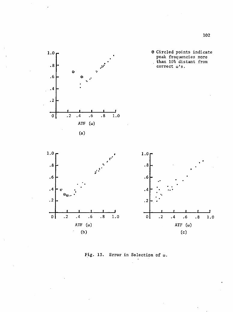
102
0 Circled points indicate . ' peak frequencies more
. • . than 10% distant from ,:•* correct to's.
Q>
©
_L -L .4 .6
ATF (u)
(a)
. 8 1 . 0
' '
.4 .6
ATF (to)
(b)
. 8 1 . 0
1 . 0
. 8
. 6
.4
. 2
.2 .4 .6 .8
ATF (u)
(c)
1 . 0
Fig. 13. Error in Selection of to.

103
entire length of the signal s(t) in place of using the local peak for
the integration time chosen. It may also be possible to improve the
selection of to by examining the symmetry of the Fourier transform;
investigation of this technique is recommended for further study (see
pitch error section for a brief description).
In summary, the peak selection ATFs are fairly accurate for weak
to moderate turbulence levels, but the errors at low ATFs are probably
not fundamental to the single channel technique and further study may
result in techniques to reduce the error.
Pitch Error
Aircraft roll and yaw have a negligible effect on the measurement
accuracy, but pitch produces a fringe shift and poses a potential error
source. A constant pitch angle is not detectable since it merely shifts
the phase constant of the signal. A constant pitch rate merely shifts
the frequency w. Pitch acceleration, however, does more damage. Pitch
is analogous in every way to image motion or wavefront tilt and osten
sibly should be easy to remove from the transfer function. Thus, if
pitch is measured with an angle sensor and recorded synchronously with
the data, then if pitch wavefront tilt were to separate in the atmo
spheric transfer function, probably approximately true, pitch could be
eliminated by dividing the computed ATF by a correction factor:
f = T T Vett>dt
(5.81)
where 0(t) = ~a A
a = angle sensor output in radians

104
The problem in this procedure is that the proper value of to is not
known a priori, and the pitch may interfere in the selection. Whether
this problem exists may, in fact, be obvious from the pitch data.
An alternate technique, slightly more tedious, is to divide the
interference (point by point) by the angle sensor output, properly
scaled:
i (27riot+Ad>+6) AiA2e
si = — t5-82' e ^ J
It is instructive to consider a single frequency component of
the pitch. In this case the interference term is:
q i _ * * i(2™t + A<J) + ©o sin pt) - AiA2e + c.c.
The Fourier transform of the pitch term is
rect jjj- (5•83)
F.T. {e P | _ Jo (Oo) 6 (v) + £ Jm(0o)6(v + mp) m = 1 m (5.84)
+ £ Jm(0o)6(v - mp)(-l)m m = 1
where the Jacobi identity has been used to express the pitch term
(Watson, 1966, p. 22). It appears that the least damage is done when
the pitch frequency is large and/or the pitch amplitude is small. Note
that when this Fourier transform is convolved with the atmospheric per
turbations, the odd m-terms can contribute to a shift of the peak; that
is, they tend to skew the atmospheric perturbations. (If the cosine
were selected for the pitch instead of the sine, no skewness would
result. )

105
If the pitch amplitude were large enough, one of the higher
m-terms could be larger than the JQ term and the peak value would not
give image quality. For example, Ji(0o) exceeds J0 (0O) at about ir/2
radians which in terms of aircraft pitch, a is only a few microradians
for a 20 cm point source separation. However, in this case, the sym
metry of the Fourier transform about to should be sufficient to deter
mine co by comparison with the angle sensor transform.
The similarity in the effect of pitch in shifting the peak and
in the effect of the atmospheric perturbations in shifting the peak is
also apparent. Once the pitch is removed it may also be possible to
select co accurately by examining the remaining symmetry of the Fourier
transform. It is clear that more work in this area is appropriate and
it is listed as recommended future work in Chapter 8.

CHAPTER 6
APPLICATION OF THE TWO POINT SOURCE TECHNIQUE TO THE MEASUREMENT OF THE PUPIL FUNCTION
The extraction of the atmospheric transfer function from the
output of a two point shearing interferometer is remarkably easy. The
extraction of the amplitude, A, and phase difference, A<j>, (from which
the phase, <J>, may be calculated) may also be possible from the output
with more complicated data processing. If this were done the experi
ment described in Chapter 5 would also be capable of measuring the pupil
function. The data processing errors, however, would increase in mag
nitude. A more reasonable approach is to use polarization coding of
the two point sources and a multichannel receiver to facilitate the
extraction of the pupil function.
The four-channel experiment described in this chapter, is still
almost identical to that described in Chapter 5. The airborne transmit
ter is the same except for the addition of a quarter wave plate in each
beam. The fringes scanned past the receiver are only a nuisance here,
to be removed in data processing since they are not used to extract the
interference term.
The receiver uses pre-detection processing; it splits the light
into four channels, each with a polarization analyzer set at a different
angle. With the analyzers set at successive 45° angles the outputs are
as follows:
106

107
S(0°) = A2 + A22 + 2A1A2cos(u)t +
S(45°) = Aj2 + A22 - 2A1A2sin((ot + A<|))
S(90°) = Ax2 + A22 - 2A1A2cos(wt + ^
S(135°) = Aj2 + A22 + 2A1A2sin(wt + A<j>)
Subtraction of alternate pairs above gives:
S(0°) - S(90°) = 4A1A2cosCo)t + A<|>)
S(135°)~ S(45°) = 4A1A2sin(o)t + A<j>)
Hence
»T • AT » ARC™
The wt term may be subtracted and Taylor's hypothesis permits the cal
culation of the phase. Similarly the modulus, A, may be extracted.
The advantages of the four-channel experiment are significant.
Data processing errors are reduced. Even though Taylor's hypothesis is
used to calculate the phase, the restrictions are less than required for
separation of the transfer function. A single successful pass with the
four-channel experiment gives the entire pupil function (one dimensional)
for that exposure time, whereas the single channel experiment yields
only one point on the transfer function per pass.
The primary disadvantage of the four-channel experiment is that
the signal level is reduced by a factor of greater than 4. In addition,
there is a new class of errors associated with the properties of the
polarization optics. The investigation of these errors is the main con
cern of this chapter. First, the treatment of the polarization aspects
of the experiment is presented in the ideal case (no errors) and the

108
system design changes and data processing additions to that already
described in Chapter 5 will be briefly covered.
Ideal Experiment
The polarization experiment has been qualitatively described in
Chapter 4. A quantitative treatment requires a vector wave approach.
At the receiver, the radiation from the two point sources is coherent
and the propagation vectors nearly coincide; thus, the problem is two
dimensional and suited to the use of the Jones Calculus (R.C. Jones,
1941).
With the Jones Calculus, the wavefront vector is resolved into
cartesian coordinates with modulus, A, and phase e:
i(2irvt + e ) i. i(2irvt + e,,) lA e x' + iA e v y J
x J y
which is represented by the matrix
ie. Ax e
ie. A e " y
The intensity is given by the sum of the squared moduli:
(6 .2 )
(6.3)
S = A 2 * 2 \ + \
(6.4)
The optical elements are represented as 2 x 2 unitary matrix
operators. Only two types of optical elements need to be considered
here: linear polarizers and linear retarders. The diagonalized form
of these matrices occurs when the "axes" of the element line up with
the x-y cartesian axes arbitrarily set up in the analysis. In other

109
words, the eigenvectors of these matrices are linearly polarized
incident beams, polarized in the x or y directions. An ideal linear
polarizer is represented by projection matrix.
In particular, a linear polarizer oriented with its transmission
axis in the x-direction has the following matrix representation (assum
ing no losses)
0
0
0 (6.5)
while a linear polarizer oriented at an angle 0 with respect to the
x-axis has the representation
[cos0 sin0 cos0 -sinG 'l o' f
sin0 cos0 0 0 -sin0 cos0 (6 .6 )
The non-ideal polarizer has the diagonalized form:
c 0
(6.7)
.where c = intensity transmission along the transmission axis
d = intensity transmission along the absorption axis
c » d
A linear retarder has the following diagonalized form:
ei6 0
-i6
(6 .8)

110
The retarder merely shifts the phase of the x-component with respect
to the y-component by 2<S radians.
assumptions. Lenses with f/numbers greater than f/4 are assumed to
have no polarization effect. Plane mirrors such as the reflecting sur
face of a beamsplitter are assumed to be linear elements with eigenvec
tors parallel to the s and p (i.e., TE and TM) vibration directions.
Mica and Quartz retarding elements are assumed to be pure linear ele
ments .
Ideal Transmitter
(from the two point sources) with opposite or orthogonal polarization
states. Left and right circular polarization is the obvious choice
since with it, the polarization state at the receiver is independent of
the aircraft orientation.
The transmitter with the Jones Calculus formalism is illustrated
in Fig. 14.
The laser output is linearly polarized. It is represented on
Fig. 14 by the vector:
where is the laser output power. A coordinate system is arbitrarily
chosen with respect to the laser output. (The choice of coordinate
system does not matter to the final output which is circularly polar
ized.) Figure 14 shows the matrix operators for the various elements
To analyze the multichannel output we make the following
The desired transmitter output is two coherent spherical waves
(6.9)

Mirror Mirror
V2 0 1
Beamsplitter
Atmosphere Atmosphere
l (kR2+<j>2)
i (kRo+((>2~7T/2)
i(kRl+<j)l) Aie (1
^iCkRi+^i+ir/2)
i CkR2+(j>2)
Receiver
Fig. 14. Ideal Transmitter

112
of the transmitter and for the atmosphere. The Jones vector for the
wave amplitude incident at the receiver is shown at the bottom.
The matrix for the ideal beamsplitter gives an even 50-50% split
of the power into two beams without affecting the polarization state.
With a real beamsplitter the split is slightly unbalanced, but in addi
tion may have a considerable retardation. Nevertheless, the ideal
matrix is a good model if the input light is linearly polarized with
the direction of polarization along an eigenvector of the' beamsplitter.
That is, the beamsplitter must be aligned so that the incident light
is polarized perpendicularly (or parallel) to the plane of incidence.
The two mirrors following the beamsplitter are similarly aligned and
hence the ideal matrix (an identity matrix) is not shown.
The ideal matrices for the quarter wave plate are shown, one
rotated -45° with respect to the incident light; the other +45°. (The
non-ideal transmitter matrices depart from the ideal case.) The atmo
sphere does not affect the polarization state of either beam (hence the
identity matrix) but does change the absolute phase differently, depend
ing on the respective path lengths, Rj and R2, and of course, the atmo
spheric turbulence contributions $1 and <j>2. The amplitudes A} and
A2 are affected by the atmospheric path and here also include the (1/R2)
intensity drop.
The final Jones vector is found by multiplying the laser output
vector by each matrix for the two separated beams and then summing the
output. Note that all the amplitude factors are included in the
and A2.
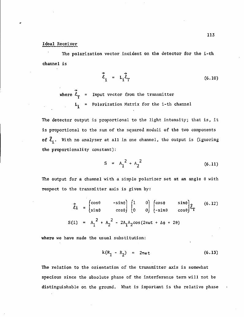
113
Ideal Receiver
The polarization vector incident on the detector for the i-th
channel is
l i ~ l i l T (6.10)
where = Input vector from the transmitter
L. = Polarization Matrix for the i-th channel 1
The detector output is proportional to the light intensity; that is, it
is proportional to the sum of the squared moduli of the two components
of With no analyzer at all in one channel, the output is (ignoring
the proportionality constant):
2 2 S = A1 + A2 C6.ll)
The output for a channel with a simple polarizer set at an angle 0 with
respect to the transmitter axis is given by:
COS0
sine
-sin©
COS0
'l O /
J 0 0
2 2 Aj + A2 - 2AjA2Cos (2irut + A<j> + 20)
l i
S(i)
where we have made the usual substitution:
k(Rj - R^) = 2iro)t
COS0
-sin©
sin0
COS0
(6 .12)
(6.13)
The relation to the orientation of the transmitter axis is somewhat
specious since the absolute phase of the interference term will not be
distinguishable on the ground. What is important is the relative phase

114
angle of the ith channel with respect to the output from another polar
izer channel with its polarizer set at a different angle. Thus we treat
the angle 0 as the polarizer angle with respect to an arbitrary receiver
axis. An obvious choice of receiver axis is the polarization (TE) axis
of the first prism used in the receiver.
The output of a left or right circular polarizer (non-linear)
will only see one or the other of the beams. The same result may be
obtained with a linear polarizer if it is preceded with a 1/4 wave
retarder to convert the circular polarization into linear:
iir/4 1 0
0 0
A,
0
-iir/4
1
-1 (6.14)
and similarly using the same quarter wave plate and an orthogonal
polarizer, only A2 remains:
iir/4 _ 0 0
0 1
'0
-1
1 - i ir /4 1 1
-1 1 (6.15)
Note that the quarter wave plate axis is rotated by 45° with respect to
the polarizer. It makes no difference what angle this pair makes with
the input beam as can be shown by the following for any 0:

115
cos0 -sin0 f y
1 0 'l -l' eiir/4 Q
sin0 cos© V. J 0 0 .1 \ 0 e"iir/4 W A
1 1
-1 1
cos9 sinQ
-sine cos0 0
(6.14)
Of the many possible receiver outputs which can be constructed
with retarders and polarizers, the three given above exhaust the sig
nificant ones, (i.e., no analyzer, a polarizer set at an arbitrary angle,
0, and a left or right circular polarizer). The receiver for the pupil
function experiment splits the input into four channels and uses a
combination of these outputs which is sufficient to permit the extrac
tion of the modulus, A1} and phase difference, A<|>.
Three different four-channel combinations which were built and
tested during this study are shown in Fig. 15. Each uses non-polarizing
beamsplitters (NPBS) to divide the incoming light equaJLly without
changing the incoming polarization state (ideally). The first two have
4 outputs of the same form: two interference terms given by polarizers
set at 0° and 45°, and an Ai2 channel and an A22 channel formed by
quarter wave plate-polarizer combination. The first uses a polarizing
beamsplitter (PBS) as the polarizer; it requires only one quarter wave
plate to serve both channels and does not lose light as with a polarizer
which absorbs the unwanted component. The second uses sheet polaroids,
throwing away half the light, but the non-polarizing beamsplitter is
less sensitive to the field angle of the incoming light. For use in a
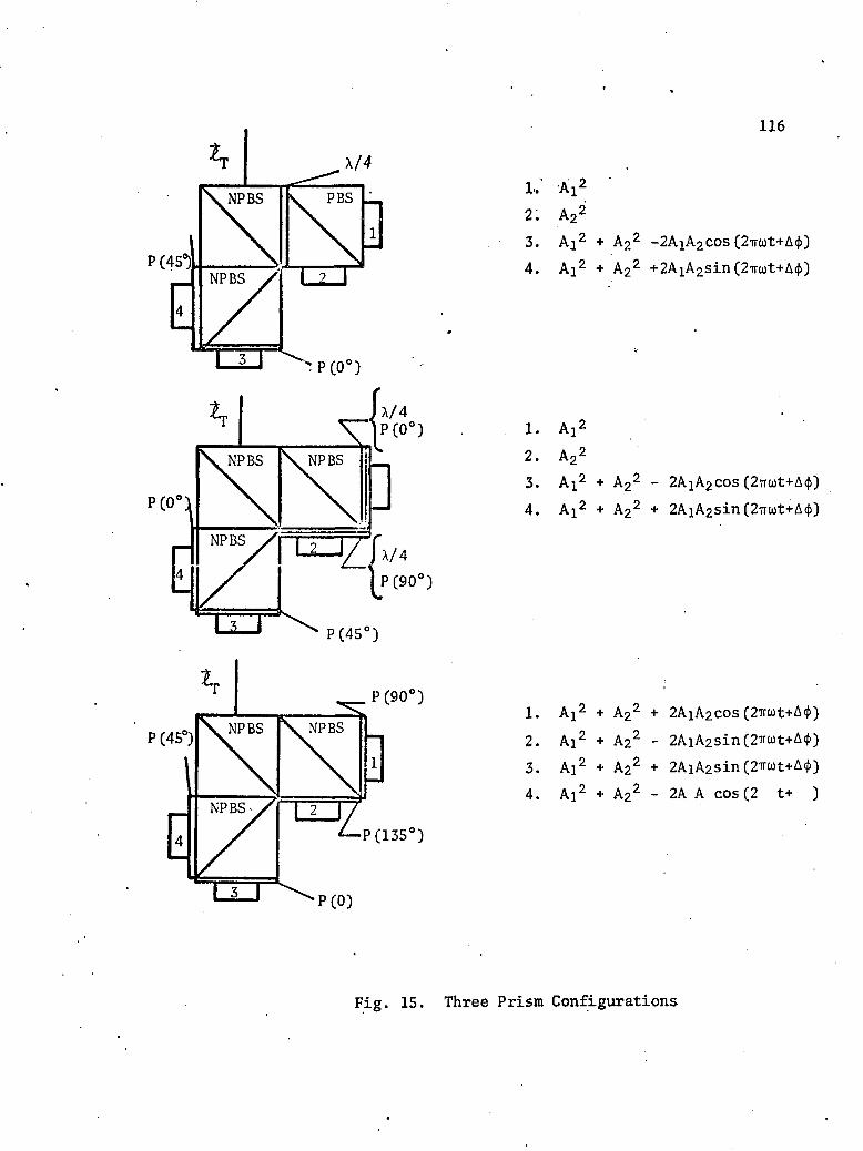
NPBS
NPBS
116
P(0°1
P(45°)
' P (0 )
V NPBS \ NPBS
^NPBS^/
A / 4
X/ 4
P (90°)
P (45 j
P (90 J
NPBS
NPBS
P (135 )
1. Ai2
2.
CM CM <
.
3. Ai2 + A22 -2AiA2COS (2TT(ot+A(j))
4. Ai2 + A22 + 2AiA2sin (2iru)t+A40
1. Ai2
2. A22
3. A}2 + A22 - 2AjA2COS (27ruyt+A<{>)
4. A12 + A22 + 2AiA2sin (27rtot+A(f))
1. A12 + A22 + 2A1A2COS (2iroJt+A(j))
2. A12 + A22 - 2A]A2sin(2,™t+A<|>)
3. A12 + A22 + 2AiA2sin (2™t+A<())
4. A12 + A22 - 2A A cos (2 t+ )
P(0)
Fig. 15. Three Prism Configurations

117
receiver with a large field angle (such as in the aircraft experiment)
the second type is preferable to the first. The third prism combina
tion, however, is the one chosen for the pupil function experiment. It
uses•four interference terms and avoids the A 2 and A22 channels. The
Aj2 and A22 channels are more sensitive to prism errors (non-ideal
elements) than the interference channels. The prism errors are dis
cussed in detail in the error analysis section to follow.
4-Channel Experiment
This experiment has essentially the same form as the transfer
function experiment described in Chapter 5. A two point source trans
mitter is carried pointed down on an aircraft, and the projected over
lapped beams are swept past a row of stationary receivers. Each re
ceiver splits the light into 4 channels. The output of each of the
four detectors is tape recorded and reduced later to give the pupil
function.
The transmitter is nearly identical to the transmitter of
Chapter 5, set for a 2 cm separation, Ax, with the addition of two
quarterwave plates, one in each beam, with axes set to produce oppo
site circular polarizations. Two quartz "double" plates (temperature
compensated) were purchased from Broomer Research for testing the pupil
function measurement (see Chapter 7). The plates are 1 inch in diameter
in order to accomodate all beam sizes.
The receivers are the same as the single channel receivers de
scribed in Chapter 5 with the addition of three prism beamsplitters and
one polaroid sheet analyzer for each channel between the field lens and

118
the detector. This placement of the beamsplitters involves a signif
icant design trade-off. Another appropriate position for the prisms
is immediately following the entrance aperture or slit. In this latter
position, however, the prisms must be much larger to accommodate the
same collecting area and must either have larger detectors, requiring
a different pre-amplifier design (and less signal-to-noise ratio), or
four optical systems instead of one. The design chosen permits more
commonality with the transfer function measurement receivers, smaller
(and cheaper) beamsplitters, and is less sensitive to background scat
ter, but the chief ray passing through the prisms is magnified by the
preceeding optics. (The angle passing through the prisms increases
the prism error.)
The prisms, or non-polarizing beamsplitters used for testing the'
experiment were thin film devices designed by Dr. Francis Turner of the
Optical Sciences Center, University of Arizona. They are described in
more detail in the error analysis section. The analyzers used were HN-38
polaroid sheet. The prisms, polaroid and detectors were cemented to form
one piece to simplify alignment procedures. The signal level for each
channel is reduced by a factor of .07 from the single channel case (due
to approximately 38% transmission of each prism and of the polaroid
analyzer). However, the bandwidth is reduced to 10 KHz (from 27 KHz)
since the to frequency at 2 cm point source separation is much reduced;
thus the resulting signal-to-noise ratio is reduced by a factor of
about .085 from the single channel case. In the data reduction, how
ever, the signals in two channels are added, which should improve the
effective signal-to-noise ratio by another factor of Jl.

119
Error Analysis
Most of the errors in the pupil function measurement must be
the same as those in the measurement of the transfer function, at
least in so far as they affect image quality. Two notable differences
are effect of noise and the prism errors, and non-ideal polarization
elements in the system.
The signal-to-noise ratio is much more critical for the pupil
function measurement. Not only is the signal level available greatly
reduced (as discussed in the last section) but the effect of the noise
is more damaging. This fact is not surprising since the pupil function
(derived from one aircraft pass) contains much more information than
one point of the transfer function. An estimate based upon using simu
lated data with the computer indicates that a signal-to-noise ratio over
the bandwidth of the receiver of 10 to 1, or 20 to 1, is required for
reliable measurement.
The polarization errors are complicated but not difficult. In
the subsections below, the receiver output errors are derived (some
times with the insight given by testing the devices built during the
study) and then followed by an analysis of their effect on the pupil
function.
Non-ideal Transmitter
The transmitter errors are very small compared to the receiver
errors and may be neglected. This is partly due to the fact that the
only components which introduce error are the quarter waveplates, but
primarily due to the fact that a very sensitive simple test is

120
available for alignment purposes. When the wave plates are adjusted
properly, the output is circularly polarized; thus a rotating polaroid
in the output beam should show no modulation in intensity of the trans
mitted beam. A one degree retardation error Cor, alternatively, approx
imately a one degree axial alignment error) produces a modulation equal
to almost 2%:
M =
2 2 M 2
cos 2
- cos 2 89 2 91 cos^ 2
+ cos^ 2
~ °'017 (6.15)
This modulation is clearly visible with the rotating polaroid test.
(Polaroid inhomogeneities are distinguishable since they give a modula
tion at one-half the frequency of the quarter wave plate error.) The
tolerance in the optical industry for fabricating quarter wave plates
is generally about A/100. However, with the rotating polaroid test
(using the laser) experience has shown that it is possible to tip the
plates and fine tune the retardation to better than ±1°. There is no
variation with field angle (a serious problem in the receiver) in the
transmitter since the angle passing through the plate is very small and
fixed.
Non-Ideal Receiver
The prism combinations in the receiver differ from the ideal
case in three ways. First, the elements themselves have errors; i.e.,
the retardation may be incorrect or some spurious dichroism may be
present. Second, the value of the retardation may change with angle;
a converging light cone is retarded differently across the cone; field
121
angle similarly changes the retardation. Last, there are fabrication
errors; the elements may not be adjusted at the proper angle. All
three of these error sources are present in the prisms constructed and
tested, but they do not affect all channels in the same way. The Jones
Calculus, here supplemented with actual measurements, is used to
analyze these effects.
Non-polarizing Beamsplitter
The non-polarizing beamsplitters used were designed by Refermat
and Turner (1971) at the University of Arizona, Optical Sciences Center,
based on their three layer thin film patent, and were fabricated at the
Optical Sciences Center. The resulting prisms were carefully selected
for low dichroism. Feedback on the dichroism measurements was used by
Dr. Turner to adjust the design. No feedback was given on the prism
retardation and the retardation of the finished prisms was quite large
(i.e., > 10° on transmission and 60° on reflection). The retardation is
so large that it is quite important to show that the retardation does not
cause an error if the polaroid is rotated to compensate for it. To do
this, we ignore (temporarily) all the other error sources and consider
only the NPBS matrix as follows for reflection and transmission respec
tively:
e ip/2 0
NPBSR = -/2
0 -ip/2 (6.16) e
NPBST = -eix/2 0
0 -ix/2 e

122
Considering first an Ai2 channel, we have the matrix operator
L(Aj) = [P(0°)3 (MICA) (NPBSR)
where
Thus
[P(0°)] =
(MICA) =
L(Aj)
1 0
0 0,
1 -1
1 1
el"/4 0
-iir/4
1^ 2
eip/2 ie~ip/2
1
-1
(6-17)
The corresponding signal out is then
S(AX2) = (1 + cosp)A12 + (1 - cosp)A22 (6.18)
- 2A^A2sinpsin(2iro)t + A<f>)
which is greatly in error.
But if the polarizer is rotated by an angle 0, then we have
L(Aj) = cos0 -sin0
sin0 cos0 P(0°)
cos0 sin©
-sin cos0 (6.19)
(MICA) (NPBSR)
The detector output is
S(Aj2) = (1 + cospcos20 - sinpsin20)Aj'
+ (1 - cospcos20 + sinpsin20)A '
(6 .20)
(sinpcos20 + cospsin20)2A1A2sin(2iTa)t + A<f>)

123
If 0 is set equal to -p/2:
sc*,*) . 4Aj2 (e . -p/2, (6 2i)
It is worth mentioning that this point is more obvious using the Poin-
care sphere representation (see Shurcliff, 1962). It is easy to visual
ize the p/2 condition and it is also obvious from the sphere that it is
essential for the quarter wave plate to be set at 45° with respect to
the axis of the NPBS in order to eliminate the retardation error by
rotating the polaroid.
An A22 beam is still orthogonal to the A12 so that the polarizer
on that channel must be rotated through the same angle from its previous
position.
The interference channels are not affected in the same way by
the NPBS retardation, but it can also be eliminated from those terms.
Note that two NPBS prisms are used in each interference channel. Thus,
if the prisms are well matched, one can be used to cancel the effect of
the other. Consider the last four-channel of Fig. 15, page 116. The
transmission axis of the polaroids are set at 0°, 45°, 90°, and 135°
with respect to the first prism axis. If the second prisms have their
axes crossed with respect to the first, then there are two channels for
which the retardations cancel: the one which is transmitted through two
prisms, and the one which is reflected at two prisms. Clearly, these
two channels should be made the 45° and the 135° channels. The other
two channels, one with a transmission followed by a reflection and the
other with a reflection first followed by a transmission, have uncan
celed retardations. However, if these are the 0° and 90° polarizers,

124
then the only part of the incident beams which get detected are eigen
vectors for both prisms and hence are not retarded.
Tests with crossed prisms show residual retardation effects
which occur with field angle variation, but this is a small error and
is discussed below.
The NPBS does exhibit a small dichroism. That is, the reflec
tance for light linearly" polarized in the s (or TE) direction differs
from the reflectance for light linearly polarized in the p (or TM)
direction. The results for transmission are similar to those for reflec
tion. Measurements indicate that s to p (or p to s) ratio on transmis
sion or reflection is typically 38%/40%. Note that the prisms are
lossey due to absorption by a silver layer. There is a variation of a
percent or so across the surface. For a circularly polarized input beam,
the polarization state shifts due to dichroism by an angle n, where
using the above typical values
A 2 A cos
2f90° - n) A cos 2 = *40
90° + n} 2 J = '
(6 .22)
which implies n = 1.5°. The matrix representation for a dichroic beam
splitter is:
m 0 NPBS = j
n (6.23)
where, for the typical values given above
m or n = .894 (6.24)
n or m = .872
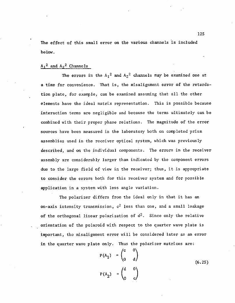
125
The effect of this small error on the various channels is included
below.
Ai2 and A22 Channels
a time for convenience. That is, the misalignment error of the retarda
tion plate, for example, can be examined assuming that all the other
elements have the ideal matrix representation. This is possible because
interaction terms are negligible and because the terms ultimately can be
combined with their proper phase relations. The magnitude of the error
sources have been measured in the laboratory both on completed prism
assemblies used in the receiver optical system, which was previously
described, and on the individual components. The errors in the receiver
assembly are considerably larger than indicated by the component errors
due to the large field of view in the receiver; thus, it is appropriate
to consider the errors both for this receiver system and for possible
application in a system with less angle variation.
on-axis intensity transmission, c2 less than one, and a small leakage
of the orthogonal linear polarization of d2. Since only the relative
orientation of the polaroid with respect to the quarter wave plate is
important, the misalignment error will be considered later as an error
in the quarter wave plate only. Thus the polarizer matrices are:
The errors in the A 2 and A22 channels may be examined one at
The polarizer differs from the ideal only in that it has an
(6.25)

126
Substituting these into the receiver matrix gives
I c ic^
^ = U d )
C6.26)
• - c : )
s(Ai2) = c2aI2 +
S(A22) = AI2 + c2A22
The polaroid causes a cross coupling due to the leakage, but
there is no interference term in the output. The Aj2 and A22 terms are
still orthogonally polarized and hence, do not interfere. All the
remaining error sources do produce an interference term. Assuming
again an ideal polarizer for these other errors, all radiation which
passes through the polarizer and reaches the detector has the same polar
ization form and hence, the wave amplitude may be expressed in scalar
form; for example, the Ai channel wave amplitude is:
|ylkRl • + (6.27)
where a and a are constants which depend on the component error. Thus,
since the output signal is proportional to the modulus square of the
wave amplitude
SfA.^) = + aA22 + a2A1A2cos(2irtot + A<j> + cO (6.28)
In general, the residual A22 term is smaller than the interference term;
usually it is much smaller. In fact, laboratory tests on the prisms
constructed with, an Aj2 and an A22 channel showed that the rejection

127
ratio, AJ2/A22J in the Aj2 channel was 100/1; i.e., a2 = .01. This
implies a signal with a 10% ripple:
It may be difficult to remove such a large ripple in data processing
since the frequency is shifting due to the influence of A<j>. For this
reason the easiest way out is to choose 4 interference channels in the
4-channel prism array, discarding the Aj2 and A22 channels altogether.
(As already mentioned the interference channel choice has a signal to
noise ratio advantage in the data reduction procedure as well.)
The errors which lead to the 10% ripple can be isolated with the
aid of the Jones Matrices.
The receiver matrices for the A12 and A22 channels modified to
account for the NPBS dichroism are as follows:
S(Aj2) = A 2 + (.01)A22 + (.l)2A1A2cos(2Tra)t + + <x) (6.29)
(6.30)
These imply the following output signals:
S(AX2) (m + n)2A 2 + (m -
2 2 - (m - n )2AjA2COS (2iuot + A<J>)
/• .2.2 - . 2, 2 (m - n) Aj + (m + n) A^ S(A22)
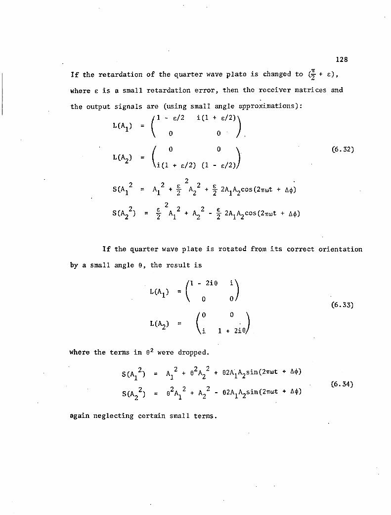
128
If the retardation of the quarter wave plate is changed to (y + e),
where e is a small retardation error, then the receiver matrices and
the output signals are (using small angle approximations):
/I - e/2 iCI + e/2)\ L(Aj)
l(A2)
o 0 / .
' 0 0 \ (6.32)
u( 1 + e/2) (1 - e/2)/
2 2 2 2 S(Aj = Aj + A2 + ^ 2AjA2cos (2Tru)t + A<|>)
2 s(a22) = | Aj2 + A22 - | 2A1A2cos(2™t + A<())
If the quarter wave plate is rotated from its correct orientation
by a small angle 6, the result is
/I - 2i0 i\
L ( V H o 0,
(0 o \ LCA2) = (
* \i i + 2iey
where the terms in 02 were dropped.
SCAj2) = Aj2 + 02A22 + 02A1A2sin(2ira)t + A4>)
S(A22) = 02Ax2 + A22 - 02A1A2sin(2ira)t + A<j>)
again neglecting certain small terms.
(6.33)
(6.34)

Combining the three error sources gives approximately:
129
where
S(Aj2)
S(A22)
a„
= A^ + a^cos(2Trut + A(j> +
2 = + a2C0sC2ira)t + A<j> + 02)
(f-4-4) -2 \ m + n /
1/2
a, = tan -1
m + n
- 0
e 2 2 2" - m + n ]
(6.35)
a„ = tan -1 -e
E + M 2
n 2 2 m + n
Typical values for the selected NPBS elements imply
4^4 - -0128 (6.36) m + n '
Misalignment errors measured for the constructed prisms were found to
be about 1 degree, or
(e) = .0174 (6.37)

130
Retardation error of the mica quarter wave plates were measured to be
about 1° (In air) on axis and up to 4° at an angle of 12° off axis.
In the receiver used, the actual reduced angles going through the prism
are spread over ±1° on axis. Off axis at the 1.5° field angle, the
angles through the prism are spread over a range from 3.5 to 8°. Thus,
as an estimate, the receiver retardation error may be expected to be
•°15 °n 3X13 (6.38)
.030 1.5° off axis
The sign of the retardation error is dependent upon the azimuth of the
field angle.
Substituting these values (arbitrarily choosing positive sign)
into the expressions for a and a gives (off axis):
a^ = .024
a2 = -046 (6.39)
a1 = -45°
a 2 = - 2 2 °
The actual measured "a" values were even greater, and were always at
least 0.1.
Interference Channels
The interference channels consist of detectors proceded by polar
izers and non-polarizing beamsplitters. Hence the desired output is
proportional to
2 2 S(t) = Aj + A2 + 2A1A2cos(2iro)t + A<|>) ^

131
as has been shown in the section on ideal receivers. If the leakage of
the polarizer, d2, is negligible, then the wave amplitude incident upon
the detector may be expressed as a scalar:
A (1 + f.)eiCkRl + *1 + a) + A,CI " T)ei(kR2 + C6-41) X & £ £»
where again a represents amplitude error due to the prism and similarly
a represents phase error.
The modulus squared is approximately
S(t) = A12(l+a) + A2(l - a) + 2AjA2(1 - a2)
(6.42) •cos(27ro)t + A(J> + a)
Thus it would seem (without considering the error sources as yet) that
the interference channels would exhibit little error in the amplitude of
the interference term with respect to Aj2 + A22, but would be expected
to show considerable error in A12 relative to A22• In fact, a = .1
implies 20% relative error in A12 with respect to A22. However, a
special condition for having negligible error is obtained by setting Aj2
approximately equal to A22:
S(t) s Ax2 + A22 + (Ax2 - A22)a + 2AjA2(1 - a2)
cos(2ira)t + A(f> + a)
(6.43)

132
The term proportional to "a" approaches zero when Aj2 approaches
A22. This condition actually occurs in the proposed experiment, since
the separation of the two point sources is quite small. Thus the error
term - A22 a is the product of two small quantities and approxi
mately equal to the interference term error, a2.
The error sources can be modeled using the Jones Calculus.
Choosing the last system picture on Fig. 15, page 118, in which the
polaroids are set sequentially at angles of 0°, 45°, 90°, and 135° we
llclVC * L(0°) = P(0°)(NPBS2T) (NPBS1R)
L(45°) = P(45°)(NPBS2R)(NPBS1R)
(6.44) L(90 ) = P(90 )(NPBS3T)(NPBS1T)
L(135°) = P(135°)(NPBS3R)(NPBS1T)
The three NPBS prisms are given additional notation above which identify
the prism number and indicate the transmission mode, T, or reflection
mode> R- , /mjRei5:iR 0 CNPBSj R) = -
\ 0 nj Re J / (6.45)
, /mjTei<S-'T 0 ' (NPBSjT). = -M
0 njTe"1
The polaroids may be assumed set at the desired angle 0 plus some small
error / 2
1 ) \sin6cos6 sin2qJ 1
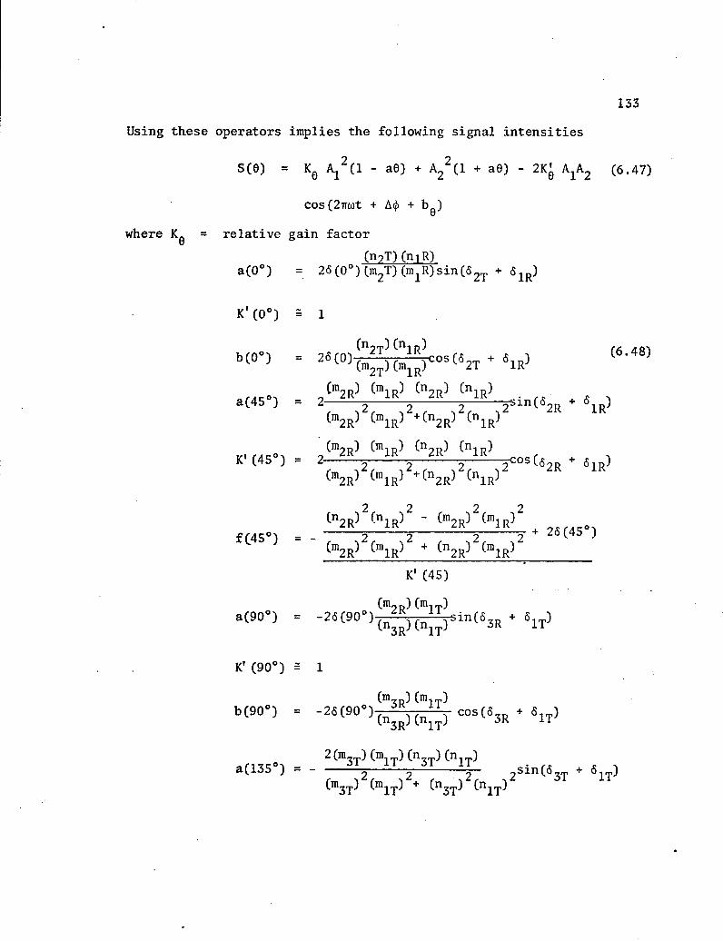
133
Using these operators implies the following signal intensities
S(0) = Kg A22(l - a0) + A22(l + a0) - 2K' (6.47)
cos(2irwt + A4> + b.)
where K0 = relative gain factor 0
(n7T)(mR) a(0°) = 26(0°)Cm2T)(m1R)sin(62T + 61r)
K' (0°) s i
,,no, , (n2T- nlR-* p . (6.48) b(0 > = (m2T)(m1R)C0S 2T + 61R^ 1 J
lM.o, ^(m2R) (m1R) (n2R) (n1R) ^ c 5 ~ , 7Tr TTZ 7T( sinC<S2R IR
2R 1R + 2R 1R
(®TD) ("MR^ ("?R^ ("l R^ t/ • / i r> O s « ^ Iv Xt\ JL X\ /• »
( ^7 727 T2COS(-<52R + ^1R (m2R) (m1R) (n2R) (n1R)
(i»2R) ("ir) " (m2R) (mlR^ 0f,jr0,
fC45° ) = - , . 2 . .2 f 2 t , 2 + 2 6 ( 4 5 ^ 2R 1R + 2R 1R
K' (45)
n) Cmi rp) a(90°) = -26(90°) Cn2 )Cn ,in(65R + 6^)
K' (90°) = 1
(^?n) (mi rp) bC90°) = -26(90°) (n ) (n|^) c0SC*3R + «1T>
f 1 , r o - v _ 2(m3T) (m1T) (n3T) (n1T)
( r >2. .2 . - 2 , 2S1 3T + IT (m3T) (m1T) + (n3T) (n1T)

134
2(m, ) (m1 ) (n ) (n ) K' (135°) = ^ 2 2COS(63T + 61T>
(m3T) (m1T) +(n3T) (n1T)
^(n3T) (n1T) - (ra3T) (m1T) ^
2 2 2 2 26 C135 ) b(135°) = Cm3T) (n1T) + (n3T) (n1T)
K'(135)
For the 45° and 135° channels the errors contributed by the NPBS
dichroism are small when typical values are considered and the results
may be simplified:
a(45°) = sin(<52R + 6^)
K'(45°) = cos(62R + SjR)
b(45°) = 26(45 ) 1 } cos(62R + 6 R)
a(135°) = -sin(S3T + 6^)
K' (135°) = cos(63T + iSjT) (6,49)
b(135°) = 26(135°) cos(63T + 6jT)
Since the prisms may be crossed, the retardation (62R + 6^R) and
(fijT + 6^T) tend to zero but have small residual values whirh increase
with field angle. Measurements on the finished receiver indicate that
|(K'-1)| is very small on axis (< .01) but increases to about .03 at 1.5°
field angle, with a corresponding change in "b" as predicted.
In the 0° and 90° cases, the retardations do not cancel, but the
K' errors are small. For misalignment of 1°, the errors to be expected
are about as follows:

135
K'(0) = K '(90) = 1 (No error)
|b CO) I = |b(90)| = .034
a(45)
a(135)
|K1 (45) - l|
|K'(135) -l|
0 on axis (6.50)
.23 off axis
0 on axis
.03 off axis
The form of the detector output with errors included is as
follows:
where G(0), A(0), K(0), and b(0) are the error terms, and N is noise.
The effect of the noise on the pupil function is more severe than it is
on the transfer function measurement, but experience in reducing data of
this nature (Gruenzel, 1975) indicates that it can be neglected when the
signal to noise (voltage) ratio is greater than 20. The gain factor
G(0) depends upon laser irradiance at the receiver which is, of course,
the same for each channel, but it also depends upon the transmission of
the prisms, the responsivity of the detectors, and amplifier gains which,
in general, may be different for each channel. Since the input signal
level is the same for each channel, the signal itself can fc-o used to
calibrate and remove the factor G(0). Integrating the signal over a
period, T, (as long as possible), gives:
s(0) = G(0){A i2[1 + a(0)] (6.51)
+ K(0)2A1A2cos(2ira)t + A<j> - 20 + b(0)| + N
(6.52)

136
where G'(0) approaches the desired factor G(0). The primary error in
G'(t) is due to the fact that the integration time may not be an integral
number of cycles of cos2irwt: the fraction of a cycle produces an
integrated value which is different for each channel. In the case of a
pure sinusoidal signal, the integrated signal is readily seen to be
G-CO) „ GCO) [l +^al] C6.53)
with similar results for the other channels. The maximum possible error
in G'(0) is equal to the local maximum of the sine function for the
approximate number of cycles integrated. For example, with only about
30 cycles integrated, the maximum error is 1/2%. (Nominally, 30 cycles
in the experiment corresponds to 50 msec, signal length.) This error
may be neglected when compared to the noise.
The remaining error terms of interest are due to the non-ideal
polarization elements in the receiver. The effect on the modulus of the
pupil function is quite small. Adding the outputs [after dropping the
G(0) factor] gives
1/2[S(0) + S(90)] = (Ax2 + A22) + (Aj2 - A22)
(a(0) 2 a(90))- 1/2 (K q - 90) [ZAjA^os (2iru)t + A«]
1/2 £S (45) + S(135)3 = (Aj2 + A,,2) + (A^ - A^) ^
(at45) * a(135) + 1/2(K45 -'K135) J^A^sin^irtot + A<|>)]
where the phase error term has been neglected since it has no serious
effect. The ripple term is very small since it depends only on the

137
modulation errors. Measurements on the assembled prisms indicate a
maximum error on the order of one or two percent in ripple.
The prism error analysis indicates that the A(0) errors are the
longest (caused mostly by residual retardation of the non-polarizing
beam splitters). Measurements of K (off axis) imply that A(0) can be
as high as 20%, although usually smaller than 10%. This could cause
some significant error in the calculation of the modulus, as reflected
in the second term (above). The fractional error given by that term is
A 2 A 2 ,
1 " 2 /a45 + al35\ 727^2 C6.SS) 1 2
2 2 Computer generated wavefronts (see Chapter 3) indicate that A^ and
are usually within 15% of one another for a 2 cm point source separation.
The resulting error term would then usually be lower than 2%. The
quality of the data can be estimated by forming the factor:
M<f>F = 1/2 [S(0) + S(90)] - 1/2[S(45) + S(135)]
However, it is possible (but not likely) for the factors A(0) to cancel
in this factor.
The phase difference errors (with errors) is given by
^ ^ . -If S(45) - S(135) | = tan Is(90) - SCO] | (6.56)
= tan •1 | Us + Ks sin(2ira)t + A(j> + b^)l { Uc + Kc cos(2iro)t + A<j> + bc) J

2 . 2\ 138 /A - A
where Ug « I^2__±_j£a(45) - a(135)J
i/a22 " aI2N Uc " ii AlA2 J[a(90) - a(0 ) ]
Ks s j[K(45) + K(135)J
Kc s l.[(90) + K(0)]
bs s b(45 + b(135)
bc s b (90) + b (0)
Ug and U£ have, of course, the same order of magnitude as the
fractional error term for the modulus already discussed. For Us and
Uc on the order of .015 or less the error in phase difference term is at
a maximum, 1° or less, when the argument, (2™t + A<j>) is an integral
multiple of TT and is zero for odd integral multiples of ir/2. The
modulation factors Kg and produce similar errors for |l - K|<.03,
but is at a maximum.

CHAPTER 7
GROUND EXPERIMENTS
Two horizontal path experiments were performed to test equipment
and techniques developed during this study. The first experiment, in
November 1974, tested the transfer function measurement. The second
experiment, in October 1975, tested the pupil function measurement. In
both of these tests, the basic motivation was to evaluate the equipment
and techniques useful for an airborne experiment and not for a horizontal
path experiment. While results for the atmosphere effects over the test
paths was not a primary goal, some of these results are given below:
Transfer Function Experiment
The transmitter described in Chapter 5 was mounted on a rotating
table on the roof of the Optical Sciences Building in Tucson, and
receivers were placed on Tumamoc Hill, 3.5 miles away, just west of the
city. The optical path was not instrumented, but it no doubt had
considerable variation in C^ and LQ.
Two receivers with 3° fields (see Chapter 5) were aligned with
respect to the static beam. The beam was swept past the receivers sig
nals, amplified, and recorded on tape.
The transmitter was first aligned statically with respect to
the receiver, then scanned past at arbitrary intervals, "on demand" by
telephone communication from the receiver site. Measurements were made
139

140
(receivers looking east) for four days from about 5:00 a.m. to about
1:00 p.m. Before dawn (about 6:30 a.m.) with a static beam, the fringes
formed by the two point sources were easily visible on the (white)
trailer at the receiver site. The intensity blobs and swirls (due to
kturbulence) in the 100-foot diameter static beam were swept by the wind
across the trailer in apparent verification of Taylor's hypothesis
(estimated velocity: 10 to 15 mph). The fringes "quivered" but were not
themselves swept across with the intensity fluctuations. Measurements
indicated that the effects of turbulence on the fringes (with rotating
transmitter) usually reached a minimum at about 8:00 a.m., and then
increased significantly with increasing sun elevation. Very heavy
scintillation was present in the late morning and early afternoon, and
false background triggers (sun glints) also began to appear.
Fig. 16 shows data from a typical pass, replayed from the tape
into an A/D converter and into the computer. The data displayed in
Fig. 16 is condensed so that each 0.1 msec time increment shown repre
sents five samples, with the stars connecting the maximum and minimum
sample values vertically. With this condensation, the fringes formed
by the transmitter with 5 cm point source separation are readily appar
ent from the figure, although only about five or ten percent of the data
train is shown. The dashed line at the bottom represents the ambient
mean from the receiver based upon samples taken immediately prior to the
pass. The average signal (arbitrary units) and the time from trigger
(in milliseconds) are printed at the bottom. The fringe period at the
receiver was 2 inches and the receiver slit width was 0.5 inches.

141
49 49
820 920
151 126 ! #*«***« 22 Nov.
50 020 151 53 120 253 i ************* Pass 9 50 220 341 j ****!*****
50 320 iOb j ************* Reel 2 50 420 251 J *;fc****.**** 50 520 160 ! ****** Ch Q 50 620 132 ! *** *********** Viiio.ii v
50 720 215 ! *************** 50 820 308 j **********4 ******* 50 920 417 j **** 51 020 355 1 *******
51 120 311 } **************** ****** 51 220 193 { **************** 51 320 147 | ******** 51 420 197 J ****** 51 520 304 | ************> '.-A +^K 51 620 422 | ********* 51 "20 450 } ****** 51 820 337 j ****-****-**** 51 920 235 } ************ 52 020 192 } ****c******** 52 120 174 | ****** 52 220 270 j ********* 52 320 415 j *********:* **.fc** 52 420 508 J ******* +TK******' r*ni<*>i.* 52 520 538 J ********* 52 620 461 | ***** !'*********** 52 720 330 | ' **tfK+**-*****H ****** 52 820 208 j *************** 52 920 131 j ******** 53 020 195 { *************** 53 120 290 J **************** * K*** 53 220 438 J ***• ******** 53 320 515 | ******** 53 420 513 j ***.****** 53 520 423 j **%•*%***:**•***•* * 53 620 255 j **************** 53 720 144 | - **:**** 53 820 166 j ***;******* 53 920 303 j *************** **• *: <** +:*-** 54 020 497 j ********************* 54 120 561 j ********c*** 54 220 525 j ************ 54 320 395 I ******* ** i*****"******* 54 420 254 | ********* 54 520 197 J ***** 54. 620 132 ! ********** 54. 720 271 j ******•>{<*********>:*:• 54. 820 375 1 *****::************ 54. 920 436 ! ********** 55. 020 497 ! **l* 55. 120 463 | *********;*******•**
Fig. 16. Condensed Data Output

142
Fourier transforms for integral multiples of 512 sample points
were calculated in order to give the ATF. Fig. 17 shows a display of
the Fourier transform calculated for nearly the entire data train (512
sample points) shown in the previous figure (Fig. 16). Only the posi
tive frequencies are shown; this figure, too, is condensed and represents
256 Fourier transform points over a frequency range of DC to 25 KHz.
(High frequencies were arbitrarily cut off in the display.) Sine inter
polation of the data was used to find the value at the peak frequency.
The ATF is given by the ratio of the peak frequency value to the half
D. C. value (see Chapter 5), and hence is approximately 60% for this
time increment.
The exposure time for 512 sample points is approximately 5 msec
with a wind velocity on the order of 10 to 15 mph, which was typical
during these tests, only about two inches of the frozen atmosphere
traversed the receiver during one such exposure time. This is not
sufficient to give a reliable ATF according to the conditions chosen
for the application of Taylor's hypothesis (Appendix I) and consequently
the ATF for 512 points must be viewed with extreme reservation. Never
theless, longer exposure times for this experiment probably contain
effects due to (unknown) non-uniform rotation of the transmitter in
addition to the desired atmospheric effects and hence, are not shown
here. This point was indicated by observation of the changes in the
peak frequency during a series of 512 point transforms. The transmitter,
although mounted on pneumatic isolators, was quite sensitive to wind

FAST FOUR I El? TRANSFORM
CHANNEL 0 HALF DC - 57304.43 PEAK » 3--I50S.95 AT 1.27 KHZ TIME - 0.05 SEC
j I j ! ! I I I j j i .
T i R ! A ! N ! S I * F ! * 0 1 * R ! * M ! *
I * V ! * A ! * L ! * U ! * E " ! *
! * ! *
!* * ! * • ** !* XcK !* Xc* !* ** ! ;k ** ! * ** !* *xc !* ** !* !* Xc !* * xc ! * xc** xobmok H xc xt 0-** -**XOMOMoW*XotcXcXoMololctolotoMtXoMoMc1<#XoKXc)!OW cXOMoMof Xol<)kXoM<-XOKXl)Wbt*)K 4 4
2 4 6 8 10 12 14 16
FREQUENCY (KHZ) £ 04
Fig. 17. Condensed Fourier Transform Computer Output.
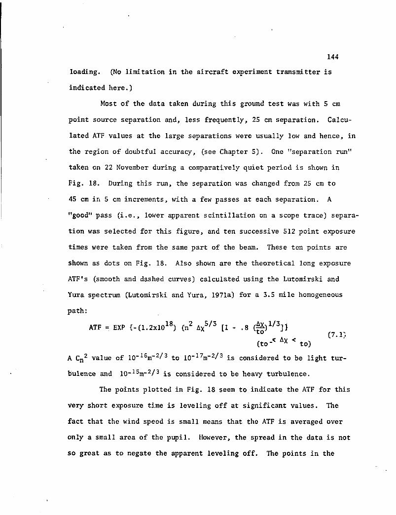
144
loading. (No limitation in the aircraft experiment transmitter is
indicated here.)
Most of the data taken during this ground test was with 5 cm
point source separation and, less frequently, 25 cm separation. Calcu
lated ATF values at the large separations were usually low and hence, in
the region of doubtful accuracy, (see Chapter 5). One "separation run"
taken on 22 November during a comparatively quiet period is shown in
Fig. 18. During this run, the separation was changed from 25 cm to
45 cm in 5 cm increments, with a few passes at each separation. A
"good" pass (i.e., lower apparent scintillation on a scope trace) separa
tion was selected for this figure, and ten successive 512 point exposure
times were taken from the same part of the beam. These ten points are
shown as dots on Fig. 18. Also shown are the theoretical long exposure
ATF's (smooth and dashed curves) calculated using the Lutomirski and
Yura spectrum (Lutomirski and Yura, 1971a) for a 3.5 mile homogeneous
path:
ATF = EXP {-(1.2xl018) (n2 Ax5/3 [1 - .8 (|^)1/3]} t0 . (7.1) (to_< x < to)
A Cn2 value of 10"16m~2/3 to 10~17m~2/3 is considered to be light tur
bulence and 10-15nr2/3 is considered to be heavy turbulence.
The points plotted in Fig. 18 seem to indicate the ATF for this
very short exposure time is leveling off at significant values. The
fact that the wind speed is small means that the ATF is averaged over
only a small area of the pupil. However, the spread in the data is not
so great as to negate the apparent leveling off. The points in the

1
3M
3x10⁻¹ u. E-<
L =10M
Separation p, or Ax, in Meters
Fig. 18. Measured Short Exposure ATFs Shown with Theoretical Curves (after Lutomirski and Yura, 1971b).
tn

146
.2 to .3 region are in the questionable accuracy range for the peak oi
selection, and this indicates possible error in all the 40 to 50 cm
shear value points.
Pupil Function Experiment
Since the pupil function experiment is identical in many features
to the transfer function experiment, the test described above applies to
both experiments. The pupil function experiment, however, differs sig
nificantly in the receiver and data processing. Although the data
processing can be easily tested with simulated wave front data, and the
receiver can be laboratory tested, a short path (600 ft.) field test
was performed in October 1975; a transmitter operating on the roof of
the Optical Sciences Center was directed on a horizontal path toward a
large mirror (flat) placed on the Space Sciences building, also located
on the University of Arizona campus. The mirror returned the beam to a
prototype 4-channel receiver and the output signals were fed to the
tape recorder.
The most critical item for test was considered to be the
signal-to-noise ratio. The calculated signal-to-noise ratio for the ATF
measurement was 30 (see Chapter 5). The receiver transmission for the
4-channel is lower by about a factor of 13- Thus, since the collecting
area is larger by a factor of four (no slit is required) and noise band
width is reduced by a factor of two, the signal-to-noise ratio for the
pupil function measurement can be estimated as about 13 for the same
beam size, receiver separation and data length used in the previous cal
culation. The beam size can be reduced slightly to insure the

147
signal-to-noise is above 20 over most of the pass, but since the cal
culated value is marginal even then, a field test is appropriate.
A special transmitter was built for the roof test and is dia
grammed in Fig. 19. The diagram is not to scale. The special trans
mitter was required to match the fringe separation in a longer path
airborne experiment. The point source separation for the roof transmit
ter is adjusted (arbitrarily small) by tilting one of the mirrors in one
arm of the Twyman-Green interferometer formed by the polarizing beam
splitter. The two interfering beams are given orthogonal linear polari
zations by the beamsplitter and these are converted to orthogonal cir
cular polarizations by the quartz quarter wave plate. The mica quarter
wave plates are required to send the two beams out through the exit face
of the beamsplitter. The lens is used to form the desired beam diameter
at the receiver. Note that the lens must be placed with the two mirrors
of the interferometer at the focal point in order for the two beams to
overlap at infinity.
The transmitter losses are about the same as for the airborne
transmitter due to the losses in the mica. Signal-to-noise measurements
showed that about 60:1 ratios were obtained with the laser output power
set at 400 mw. This is consistent with the calculated value.
The beam diameter was set at 110 feet at the receiver with about
18 inches fringe period. This implies that the point source separation
was 0.5 mm, smaller than the inner scale of turbulence. Consequently,
very little atmospheric turbulence effect was expected.

148
Laser
- [ J
Beam Expander
• -0-Q
i •
i
} Mica A/4 Plates Beamsplitter
Quartz A/4 Plate
Lens (47mm f1.)
Point Sources
Fig. 19. Roof Transmitter.

149
Figure 20 shows a typical phase difference output derived from
the experiment. The transmitter was held stationary during this "pass"
The transmitter was also rotated during the roof test, but the results
clearly show transmitter vibration effects and perhaps beam irregulari
ties .

CCNTEKCD FM»VX DJIR^CUTT PLOT HI UMIRI Tiff!
o.mm'.S O.M Wi c.bi3r.r» O.M4m O.M*/VR, 0.5 IW, e.5K O.M«VJ15 o.sirw? o.5K;225 O.SI '.O 0.51*505 0.520U5 o.52or?.5 0.5?1425 0.5220*5 0.522/05 0,5?33t5 0.523>05 0,52.1625 o.52s:r5 a,5?5r05 0.52C545 0.5271S5 0.52?r25 0.5234*5 0.529100 0.523745 0.530335 0.531025 0.53IC65 0.532305 0.5329-15 0.533505 0.534225 0.53- oS 0.535505 0.53f.l-i5 0.536725 o*537425 0.53SC-:5 0.533705 0.5393-15 0.539735 0.540*25 0.541255 0.541505 0.542545 0.545185
pjiftf.r DJFF cijr.v* %\ -fl.ot.v -n.oi'.M •P.ni:;2 -0.0214 -0.OUHI -0.01ir -0.0073 -P.INMJ -O.OPC4 -n.»ni7 -0 .0122 -0.0083 -o.i <ro2 -0.010? -0.01Q4 -0.0110 -0.0100 -o.otrs 0.0002 -0.0055 -0.0U92 •0.015-3 -0.0133 -0.0032 -0.0023 -0.0073 -o.ooeo -O.0066 -0.0133 -0.0052 -O.OOOo -0.0003 ~o.co72 -0.0132 -0.C21O -o.o:oa -0.0215 -0.0179 -0.0135 -0.0205 -0.0201 -0.0273 -0.0342 -0.0231 -0.0152 -0.0126 -0.012C -0.0181 -C.C S3
-1.0 e.e i.o
s P < <D to
s p < (D to
in o
Fig. 20. Phase Difference, Stationary Transmitter
CHAPTER 8
CONCLUSIONS AND RECOMMENDATIONS
The feasibility of an airborne experimental program for measur
ing the atmospheric part of the transfer function and of the pupil
function has been proved by analysis and by testing the equipment to be
used in such a program over a horizontal test path. Although the fact
that the transfer function separates into an atmospheric factor has not
been conclusively proven for all cases of interest, the indications of
separation for the airborne experiment are so strong as to suggest that
any resultant error in applying the measurement to intermediate exposure
times is well within experimental tolerances.
The transfer function measurement is more subject to error than
the pupil function measurement at this time. This fact is especially
due to the errors in separating the normalization term from the inter
ference term and in selecting the proper heterodyne frequency to use
in the data reduction. The errors are worse for low values of the ATF.
The pupil function measurement is less susceptible to error but
slightly more difficult and requires a greater signal-to-noise ratio.
The pupil function measurement is much more complete for the same
amount of raw data.
151

152
Modeling the atmosphere for theoretical calculations of image
quality is very difficult. There are indicateions that the theory of
homogenous turbulence rarely applies over real atmospheric paths of
interest (except for specially selected test paths). Also the ensemble
average image quality data that the theory predicts has no direct appli
cation to the intermediate exposure times frequently used. The indirect
use of the ensemble average answers to generate random sample functions
for simulation of intermediate exposure times has been more useful in
this study in providing testing for the experimental data processing
techniques than it has been in learning about the atmospheric effects.
Many of the obvious recommendations for future work based upon
this report alone have in fact already been done during this study by
co-workers of this writer, such as the difficult but important aircraft
qualifying of the laser-transmitter package and its isolation from air
craft vibration; also the electronics mechanics and information display
to the pilots for timing the laser in flight, for changing lenses and
point-source separation in flight, etc., as well as the many refinements
of the electronics at the receiver. The data processing and programming
have been and are being substantially improved.
The following specific recommendations are made:
1. Separation of the transfer function. The sample function tech
niques discussed in Chapter 3 can, if extended to two dimen
sions provide a test of the separation of the transfer due to
Taylor's hypothesis. Actual camera designs could be used in
this test.

153
Selection of w for the transfer function measurement. The use
of the Fourier Transform symmetry may possibly provide a
better selection of to than currently available and should be
developed.
Extraction of the pupil function from the single channel data.
Non-linear data reduction techniques may permit extraction of
the phase from a single channel output. The extent of the
errors should be evaluated.
A fixed horizontal path experiment. In many ways a fixed
horizontal path experiment is easier to perform and more
accurate than the airborne experiment. Although it is not
productive of vertical path data, frequency monitoring of
a long horizontal path would provide useful optical data
which can be correlated with monitoring equipment along the
path.
Depolarization by atmospheric turbulence. Theoretically and
by some limited experiments this is felt to be negligible.
The present technique permits a critical measurement of this
to be carried out.

APPENDIX I
THE SEPARATION OF THE OPTICAL TRANSFER IN A TURBULENT MEDIUM
Qualitative Remarks
The optical transfer function does not generally separate into
two independent factors, although there are a few familiar exceptional
cases. The most important example of the transfer function not separa
ting is probably its failure to cascade through a series of optical
elements as does the electronic transfer function through, say, a series
of amplifiers. Optical design often uses the ability to correct or
balance aberrations in one element with those in another which would be
impossible if the transfer functions for the two elements multiplied.
The most familiar example of separation is in the case of weak
aberrations. The effect of weak aberrations on the transfer function or
the image is relatively independent of the type of aberration, i.e.,
independent of its distribution in the pupil. This fact is embodied in
the long used concept of the Strehl Ratio (Born and Wolf, 1965, p. 381).
It is extended below to cover the case of weak turbulence.
Strong turbulence separation is also discussed (somewhat loosely)
below. However, the case of strong turbulence seems to be of the least
interest since the image quality is poor in any event.
Another familiar exceptional case in the theory of image forma
tion is the separation due to image motion. The image motion usually
considered in the theory occurs at a uniform velocity over the exposure
154

155
simplifying the analysis, but separation of the transfer function is
not limited to that restriction. The effective psf for the exposure
is the optical system psf or impulse response convolved with the time
history of the image motion; separation of the transfer function into
a factor which depends only on the optical system and a factor which
depends only on the image motion follows the convolution theorem.
Image motion produced by turbulence is called image dance or agitation
and is not uniform in velocity. It is caused by large scale turbulence,
i.e., turbulent cells large with respect to the aperture. Motion of the
image is equivalent to a tilt of the pupil function or wavefront. Wave-
front tilt due to turbulence has been studied theoretically (Fried,
1966a; Yura, 1973). A significant part of the theoretical long exposure
transfer function (i.e., ensemble average) is often caused by wavefront
tilt.
A last familiar case for separation applies to the long exposure
transfer function in a turbulent medium with time varying wavefronts
(O'Neill, 1963; Hufnagel and Stanley, 1964; Fried, 1966b). This separa
tion is actually a special case of a more general condition which can be
applied in a different way with the aid of Taylor's hypothesis. With
f.ime varying wavefronts the effective transfer function is proportional
to the sheared pupil function integrated over the aperture and then
integrated over the exposure time. Formally, however, the order of inte
gration may be interchanged so that the transfer function is proportional
to the sheared pupil function at one point in the aperture, integrated
over time and then integrated over the aperture. The atmospheric part

156
of the transfer function is separable if the time integration for one
point in the aperture is independent of the position in the aperture.
It follows that if each point of the aperture sees the same instantaneous
values of the sheared pupil function Cm whatever order) over the expo
sure time, then the transfer function separates. One way to insure
(formally) that each point of the aperture sees the same values is to
impose the condition that each point sees all possible members of the
statistical ensemble which describes the current state of turbulence;
i.e., each point sees the ensemble average value of the sheared pupil
function, assuming that an ergodic, stationary random process is a valid
representation of the turbulence. This is a statement of the long expo
sure separation condition. The ensemble average condition, while suffi
cient for separation, is often mistakenly treated in the literature as
if it were a necessary condition.
Separation due to image motion or wavefront tilt can be inter
preted as a trivial example of the more general condition for separation.
Wavefront tilt produces a contribution to the phase of the sheared pupil
function which is constant over the whole aperture. Thus, each point of
the aperture sees the same values of the sheared pupil function due to
wavefront tilt (in this case in exactly the same order) over the exposure
time for any exposure time. It is tempting (and probably correct) to
speculate that the large scales of turbulence which cause wavefront tilt
take the longest time to reach an ensemble average value of the sheared
pupil function; thus, effective separation of the transfer function would
occur much quicker than the ensemble average condition implies.

157
Separation in one dimension for all scales of turbulence occurs if
Taylor's hypothesis is applied to describe to the time varying wave-
fronts; then the sheared pupil function is "frozen" and is swept across
the pupil by the wind. Each point in the aperture then sees the same
values of the sheared pupil function as any other point with the same y
coordinates (wind in the x-direction) except for the end points. Thus,
if the exposure time is long enough to reduce the effect of the end
points, the transfer function for a camera with a strip aperture in the
X-direction clearly separates. Separation in the y-direction follows
also, but with less rigor. At least, the width of the strip need not
necessarily be small. The sheared aberration function, integrated in
strips along x can often be only a weak function of y over much of the
aperture (e.g.,spherical aberration) so that given separation in the
x-direction the optical system itself provides some measure of separation
in the y-direction (assuming that the wind is in the shear direction).
However, the atmosphere also provides for some y-separation. If the
strip were sufficiently long, then of course separation in y would occur
eventually by ensemble averaging (the long exposure case), but effective
separation probably occurs much quicker. Small scale effects no doubt
reach a local average very quickly; large scale effects separate anyway;
the intermediate scale perturbations, approximately the size of the
aperture, are the slowest to approach a local average value. Thus, to
insure a favorable change for separation of the transfer function, the
exposure time should be long enough to give a strip in the x-direction
that is much longer than the aperture width., i.e., about three times as

158
large. This is the condition on exposure time used in designing the
experiment described in Chapter 5. Recommendations for testing this
condition with computer generated random wavefronts are given in
Chapter 8.
Weak Turbulence
The OTF in terms of the sheared exit pupil, with atmospheric
phase perturbations and optical system aberration function W is as
follows:
n-ri? /-AV A i + 2irAW) OTF (Ax,Ay) » -g-JJe dxdy CAtl)
00
V«ith the terms as defined in Chapter 1. The modulus of the perturbed
wave amplitude is ignored in this expression under the assumption that
its effects are small compared to that of the phase perturbations.
By defining the quantity AG and factoring out the average value of AG
by the OTF can be expressed as
OTF (4x,4y) .
00
AG = A$' + 2irAW (A. 2)
AG = JjAGdxdy
00
The weak turbulence separation (if AlV is also small) then follows along
the lines of Hopkins treatment of permissible optical aberrations
(Hopkins, 1957) with AG taking the place of Hopkins sheared aberration

159
function. Thus, if AG is small, the higher order terms in the expan
sion of the exponential can be neglected to give:
ei A G f f l + i(AG - AG) - (AG - AG) dxdy f OTF (Ax, Ay) = -g- J J
00
The imaginary part of the integral vanishes, and the result is
OTF (ta.ijr) = e^.[f|dxdy] [l - 4Grms*]
00
where AGrms = jj AG - AG)2dxdy (A.4)
00
JJdxdy
00
Since it is the root mean square value of AG which appears, the effect
of the distribution of turbulence in the pupil is very small (assuming
that AGrms is relatively constant in various regions of the pupil) and
transfer function separates.
Strong Turbulence
Studies of propagation through <urbulence (see Chapter 2) have
shown that the correlation distances of the wave structure function
decreases rapidly with the strength of turbulence. Thus, for example,
Fried1s parameter, rQ, (Fried, 1966a) a correlation distance of a sort,
is itself a measure of the turbulence strength. Under these circum
stances, even the instantaneous wavefront and A4>' can be considered to
be rapidly changing with distance. If A4>' can be considered to be
rapidly changing across the aperture, then it is almost always rapidly

160
changing with respect to Aw, and the OTF approximately separates as
follows:
OTF = ± D
jjelA$'dxdy 00
Jjdxdy
00
f f j le dxdy
00
CA.5)
Frozen Wavefronts
A simplification in the transfer function occurs when the temporal
changes in the wavefront intercepted by the optical system is described
by Taylor's hypothesis. Temporal changes in the turbulent structure
depends upon balancing inertial forces with viscous forces; they occur
relatively slowly. In the presence of a wind with velocity greater than
about 2 meters/second, (Clifford, 1971), the turbulent structure may be
considered to be a frozen medium that is swept past the optical system by
the wind; that is, the temporal changes are dominated by the effects of
an average wind.
The time integral contained in the OTF expressions becomes (with
a frozen atmosphere)
/: pa(x - ut,y)pa (x - ut - ARNx,y - XRN )dt (A. 6)
which for simplicity can be written
!T Jo g(x - ut,y)dt
(A. 7)

161
or, rewriting
| g l ( i - t,y)dt (A8)
* o
if x/u <<T, then the above integral is approximately independent of x:
(T ,T J t,y)dt 5 J g1(t,y)dt (smaller)
o o
Then the OTF separates in the x-direction, but possible y-variations
remain.
0TF " jf'fs'(t,y)dt Jeb*to( x , y , x)dx
•yi°
,xi ai2
dy (A. 10)
Separation in Y-Direction due to Small Optical Aberrations
The aberration free transfer function fails to separate from
the turbulence effects (except for weak turbulence) but the reason is
subtle. For a given shear value, say Ax, the aberration function is
constant (i.e., zero) over the whole non-zero part or overlapped part of
the pupil and the rearrangement of turbulent cells within that region can
have no effect on the transfer factor for that Ax. But since the overlap
region covers different parts of the full aperture for different Ax
values, rearrangement of the turbulent cells over the full aperture can
affect the transfer function. Much of this objection is removed by the
one-dimensional separation due to Taylor's hypothesis for the special
case of the shear taken in the wind direction. (This special case
coincides with the measurement geometry used in Chapter 5.) For almost

162
all shear values the integrated sheared pupil function covers nearly
the same y values and the transfer function approximately separates for
any level of turbulence. This separation can be extended to cover a
well corrected optical system (weak aberrations) as well as an aberra
tion free s>*stem. This is, so long as the x-integrated optical system
sheared pupil function is only weakly varying in the y-direction, the
transfer function separates; this separation is clear, formally, from
the last equation above. Thus, even though the aberrations are strong
enough to show considerable variation across the pupil, separation still
occurs if the variation is smoothed out by the one dimensional integra
tion.

REFERENCES
Barakat, R. (1971), Optica Acta 18^:9, 683-694.
Barakat, R., and E. Blackman (1973), Optica Acta. 20:11, 901-912.
Beran, M. J. (1967), IEEE TRANS. Ant. Prop. AP-15, 66.
Beran, M. J. (1970), J. Opt. Soc. Am. 6£:4, 518-S21.
Beran, M. J., and T. Ho (1969), J. Opt. Soc. Am., 59_, 1134-1138.
Beran, M. J., and A. M. Whitman (1971), J. Opt. Soc. Am., 61:8, 1044-1050.
Bertolotti, M., M. Carnevale, B. Crosignani, and P. Di Porto (1969), Appl. Opt. £:6, 1111-1113.
Bertolotti, M., M. Carnevale, L. Muzii, and D. Sette (1968), Appl. Opt. J}ll> 2246-2251.
Bertolotti, M., M. Carnevale, L. Muzii, and D. Sette (1970), Appl. Opt. 9:2, 510-512.
Bertolotti, M., M. Carnevale, L. Muzii, and D. Sette (1974), Appl. Opt. L3:7, 1582-1585.
Born, M., and E. Wolf (1965), Principles of Optics, 3rd Edition, Pergamon Press, London.
Bourcius, G. M. B., and S. F. Clifford (1970), J. Opt. Soc. Am. 60:11, 1484-1489.
Breckenride, J. (1975), J. Opt. Soc. Am. 65_:7, 755-759.
Bufton, J. L. (1973), Appl. Opt. 12:8, 1785-1793.
Bufton, J. L., and Genatt (1971), Astron. J. 76^:4, 378-386.
Bufton, J. L., P. 0. Minott, M. W. Fitzmaurice, and P. J. Titterton (1972), J. Opt. Soc. Ac. 62:9, 1068-1070.
Burlamacchi, P., A. Consortini, and L. Ronchi (1967), Appl. Opt. 6, 1273.
Buser, R. G. (1971), J. Opt. Soc. Am. £1:4, 488-491.
163

164
Buser, R. G., and G. K. Born (1970), J. Opt. Soc. Am. 6£:8, 1079-1084.
Chandrasekar, S (1952), Monthly Notices Roy. Astron. Soc., 112, 475-483.
Chernov, L. A. (1960), Wave Propagation in a Random Medium, McGraw-Hill, New York.
Clifford, S. F. (1971), J. Opt. Soc. Am. 6^:10, 1285-1292.
Clifford, S. F., G. M. Bourcius, G. R. Ochs, and M. H. Ackley (1971), J. Opt. Soc. Am. 61^:10, 1279-1284.
Consortini, A. (1974), Paper WB7, Digest of Technical Papers, Topical Meeting on Optical Propagation through Turbulence, July 9-11, U of Colo., Boulder, Colo.
Consortini, A., L. Ronchi, and E. Moroder (1973), J. Opt. Soc. Am. 63:10 1246-1248.
Coulman, C. E. (1965), J. Opt. Soc. Am. 55:7, 806-812.
Coulman, C. E. (1966), J. Opt. Soc. Am 56:9, 1232-1238.
Fante, R. F., and J. L. Poirier (1973), Appl. Opt. 12_:10, 2247-2248.
Farhat, N. H., and A. B. DeCou (1969), J. Opt. Soc. Am. 5£:11, 1489-1490
Fried, D. L. (1965), J. Opt. Soc. Am. 56:11, 1427-1435.
Fried, D. L. (1966a), J. Opt. Soc. Am. 56, 1373-1379.
Fried, D. L. (1966b), J. Opt. Soc. Am. 56, 1380-1384.
Fried, D. L. (1967), Proc. IEEE 55:1, 57-67.
Fried, D. L., and H. T. Yura (1972), J. Opt. Soc. Am. 62, 600-602.
Gaskill, J. D. (1969), J. Opt. Soc. Am. 59:3, 303-318.
Golden, L. J. (1975), Appl. Opt. .14:10, 2391-2399.
Goodman, J. W. (1968), Introduction to Fourier Optics, McGraw-Hill, New York.
Gruenzel, R. R. (1972), Application of Lateral Shearing Interferometry to Stochastic (Ransom) Inputs, Master's Thesis, Univ. of Ariz.
Gruenzel, R. R. (1975), Private Communication, Air Force Avionics Lab., Wright Patterson AFB, Ohio.

165
Herrick, R., and I. Meyer-Arendt (1966), Appl. Opt. 5^, 981.
Hopkins, H. A. (1957), Proc. Phys. Soc. B, 70, 449-470.
Hufnagel, R. E. (1966), Restoration of Atmospherically Degraded Images, Woods Hole Summer Study, Mass., National Academy of Sciences, Wash. D.C., Appendix 3, Vol. 2.
Hufnagel, R. E. (1974) Paper VTAi, Proc., Boulder Conf. on Atmospheric Propagation, Boulder, Colo.
Hufnagel, R. E., and N. R. Stanley (1964), J. Opt. Soc. Am. 54:1, 52-61.
Jones, R. C. (1941), J. Opt. Soc. Am. 31_, 488-493.
Kelsall, D. (1973), J. Opt. Soc. Am. 1_1, 1472-1484.
Lee, R. W., and J. C. Harp (1969), Proc. IEEE 57:4, 375-407.
Lutomirski, R. F., and R. G. Buser (1973), Appl.Opt. 12.:9, 2153-2160.
Lutomirski, R. F., and H. T. Yura (1971a), J. Opt. Soc. Am. 61^ 482-487.
Lutomirski, R. F., and H. T. Yura (1971b), Appl. Opt. 10:7, 1652-1658.
Meinel, A. B. (1960), Chap. 10 of Telescopes ed. by Kuiper, G., and B. Middlehurst, Univ. of Chicago Press, Chicago.
Oliver, B. M. (1965), Proc. IEEE 5_3:5, 436-460.
O'Neill, P. L. (1963), Introduction to Statistical Optics, Addison-Wesley, Reading, Mass.
Papoulis, A. (1965), Probability Random Variables, and Stochastic Processes, McGraw-Hill, New York.
Philbrick, R. G. (1975), Unpublished Data, Opt. Sci. Center, Univ of Ariz.
Ramsay, J. V., and H. Kobler (1962), Observatory 82, 107.
Refermat, S. J., and A. T. Turner (1971), U. S. Patent No. 3,559,090.
Roddier, C., and F. Roddier (1973), ,T. Opt. Soc. Am. 6_, 661-663.
Ruina, J. P., and C. M. Angulo (1963), IEEE Trans. Ant. and Prop., 153-161.
Shack, R. V. (1966), Restoration of Atmospherically Degraded Images, Woods Hole Summer Study, Mass., National Academy of Sciences, Wash., D. C.

166
Shack, R. V. (1967), Univ. of Ariz. Opt. Sci. Center Tech. Rpt. No. 19.
Shack, R. V. (1968), Univ. of Ariz. Opt. Sci. Center Tech. Rpt. No. 32.
Shannon, R. R. (1971), Univ. of Ariz. Opt. Sci. Center Newsletter _5:1, 16-19.
Shapiro, J. H. (1971), J. Opt. Soc. Am. 61_:4, 492-495.
Shurcliff, W. A. (1962), Polarized Light; Production and Use, Harvard U. Press, Cambridge, Mass.
Stock, J., and G. Keller (1960), Chap. 9 in Telescopes, ed. by G. Kuiper and B. Middlehurst, Univ. of Chicago Press.
Stone, J. M. (1963), Radiation and Optics, McGraw-Hill, New York.
Strohbehn, J. W. (1966), J. of Geo. Phys. Res. 71:24, 5793-5808.
Strohbehn, J. W. (1968), Proc. IEEE 56:8, 1301-1318.
Strohbehn, J. W. (1970), Proc. IEEE ,58:10, 1523-1545.
Strohbehn, J. W. (1971), Chap. 3 of Progress in Optics, ed. by E. Wolf, Am. Elsevier., New York.
Sutton, G. W. (1969),J. Opt. Soc. Am. 59:1,. 115-116.
Tatarski, V. I. (1961), Wave Propagation in a Turbulent Medium, McGraw-Hill, New York.
Taylor, R. J. (1958), Aust. J. Phys. 2^:2, 168-176.
Yura, H. T. (1972), Appl. Opt. 11;6, 1399-1406.
Yura, H. T. (1973), J. Opt. Soc. Am. 63:5, 567-572.
Watson, G. N. (1966), Theory of Bessel Functions, 2nd Ed., Cambridge, 1966.
Wolfe, W. L. (1965), Handbook of Military Infrared Technology, U. S. Printing Office, Wash., D. C.


