Download - WORKPLACE KNOWLEDGE FLOWS

NBER WORKING PAPER SERIES
WORKPLACE KNOWLEDGE FLOWS
Jason SandvikRichard SaoumaNathan Seegert
Christopher T. Stanton
Working Paper 26660http://www.nber.org/papers/w26660
NATIONAL BUREAU OF ECONOMIC RESEARCH1050 Massachusetts Avenue
Cambridge, MA 02138January 2020
We thank seminar and conference participants at the Academy of Management, Ammersee Workshop, Barcelona GSE Summer Forum, BEPE Chile, McGill, Minnesota Carlson, NBER Organizational Economics, SIOE, and Strategy Science, along with Karen Bernhardt-Walther, Nick Bloom, Jen Brown, Zoe Cullen, Miguel Espinosa, Guido Friebel, Bob Gibbons, Ben Golub, James Hines, Mitch Hoffman, Larry Katz, Bill Kerr, Ed Lazear, Josh Lerner, Yimeng Li, Derek Neal, Luis Rayo, John Roberts, Ben Roth, Raffaella Sadun, Scott Schaefer, Kathryn Shaw, Orie Shelef, Andrei Shleifer, and Jason Snyder for helpful comments. We thank our respective universities for research support. The views expressed herein are those of the authors and do not necessarily reflect the views of the National Bureau of Economic Research.
NBER working papers are circulated for discussion and comment purposes. They have not been peer-reviewed or been subject to the review by the NBER Board of Directors that accompanies official NBER publications.
© 2020 by Jason Sandvik, Richard Saouma, Nathan Seegert, and Christopher T. Stanton. All rights reserved. Short sections of text, not to exceed two paragraphs, may be quoted without explicit permission provided that full credit, including © notice, is given to the source.

Workplace Knowledge FlowsJason Sandvik, Richard Saouma, Nathan Seegert, and Christopher T. StantonNBER Working Paper No. 26660January 2020JEL No. J24,L23,M12,M5,M52,M53,M54
ABSTRACT
What prevents the spread of information among coworkers, and which management practices facilitate workplace knowledge flows? We conducted a field experiment in a sales company, addressing these questions with three active treatments. (1) Encouraging workers to talk about their sales techniques with a randomly chosen partner during short meetings substantially lifted average sales revenue during and after the experiment. The largest gains occurred for those matched with high-performing coworkers.(2) Worker-pairs given incentives to increase joint output increased sales during the experiment but not afterward. (3) Worker-pairs given both treatments had little improvement above the meetings treatment alone. Managerial interventions providing structured opportunities for workers to initiate conversations with peers resulted in knowledge exchange; incentives based on joint output gains were neither necessary nor sufficient for knowledge transmission.
Jason SandvikDepartment of FinanceTulane [email protected]
Richard SaoumaEli Broad School of BusinessMichigan State [email protected]
Nathan SeegertUniversity of UtahDepartment of FinanceSpencer Fox Eccles Business Bldg. Room 11131655 East Campus Center DriveSalt Lake City, Utah [email protected]
Christopher T. Stanton210 Rock CenterHarvard UniversityHarvard Business SchoolBoston, MA 02163and [email protected]
A randomized controlled trials registry entry is available at https://www.socialscienceregistry.org/trials/2332

1 Introduction
The best workers in many firms substantially outperform others (Lazear, 2000; Mas and
Moretti, 2009; Bandiera et al., 2007; Lazear et al., 2015; Lo et al., 2016). Is this due to
variation in natural abilities, or differences in knowledge about how to perform a job? To
the extent that knowledge differences matter, what slows the diffusion of knowledge among
coworkers? The literature on peer effects suggests that spillovers operate powerfully in-
side firms (Mas and Moretti, 2009; Bandiera et al., 2010), but the conditions for knowledge
spillovers and the management practices that facilitate them are less clear.1 Few controlled
experiments assess knowledge spillovers under different management practices, and obser-
vational approaches can be challenging due to omitted variable bias (Manski, 1993; Glaeser
et al., 2003; Guryan et al., 2009). To overcome these challenges, we worked with a sales firm
to conduct a field experiment.
The experiment occurred in an inbound sales call center where workers (“agents” in the
firm’s terminology) sell television, phone, and internet services to customers calling from
across the United States. Calls are allocated to agents randomly, meaning that everyone
within a division faces the same distribution of sales opportunities, and agent compensation
depends on individual performance. Using the firm’s focal performance measure, revenue-
per-call (RPC), sales productivity across agents varied dramatically prior to the experiment.
Those at the 75th percentile of the distribution brought in approximately 48% more rev-
enue on a given call than those at the 25th percentile, even after adjusting for sampling
variation. Manager interviews and agent surveys cite varying knowledge of sales techniques
as contributing to this dispersion, consistent with the importance of task-specific human
capital (Gibbons and Waldman, 2004). For example, the most successful agents understand
when and how to ask about customer needs; they know which products to bundle; they
incorporate add-ons that increase revenue; and they redirect callers to feasible alternatives
whenever they fail to qualify for specific products or promotions.
What limits the diffusion of this knowledge between coworkers? Knowledge seekers may
face initiation costs that prevent them from gathering information. These costs include so-
cial concerns (e.g., reluctance to approach unfamiliar coworkers or a fear of signaling incom-
petence (Chandrasekhar et al., 2016; Edmondson and Lei, 2014)), coordination difficulties
(e.g., setting up meetings), and search frictions (e.g., knowing whom to ask (Boudreau et al.,
1Spillovers have been shown to drive productivity growth (Marshall, 1890; Jacobs, 1969; Glaeser, Kallal,Scheinkman, and Shleifer, 1992; Barro, 1991; Romer, 1990), and there is a long history of work connectingthe transfer of knowledge to physical proximity. A common view is that firms exist to facilitate best practiceadoption and knowledge spillovers (Grant, 1996). However, there is often conflicting advice in academic andexecutive-focused publications on how to enable knowledge sharing within firms (Myers, 2015).
1

2017)). On the other hand, knowledge providers may lack the incentive to share knowledge,
due to contracting costs. In many sales firms, including this one, a portion of compensation
depends on (coarse) performance relative to other employees, potentially increasing oppor-
tunity costs of helping others. Contracting costs limit the ability of knowledge seekers to
sufficiently compensate knowledge providers for exchanging information.2
The experiment was designed to assess the effectiveness of management practices that
target initiation costs, contracting costs, and the combination of both costs. In the firm’s two
main offices, 653 agents were assigned to four treatment cells using a clustered design based on
the identity of their sales manager. Treatments occurred during a four-week period, labeled
the intervention period. At the onset, agents were all paired with a randomly assigned partner
from the same treatment, with some pairs rotating to new partners at the beginning of each
subsequent week. Agents in the Internal Control group were paired and had their joint
revenue-per-call gains (relative to the two weeks prior to the intervention period) displayed
publicly, but they were given no additional incentives or instructions to take further actions,
making them “passive pairs.” Three “active” treatments added additional layers on top of the
partner pairings. The first active treatment, labeled Structured-Meetings, targeted initiation
costs by encouraging worker-pairs to meet early in the week. Worksheets guided these agents
to reflect on their own sales strengths and challenges and to seek and record advice from their
partner.3 Pairs completing worksheets were encouraged to meet again over a catered lunch
near the end of the week. The second active treatment, labeled Pair-Incentives, targeted
contracting costs by providing paired agents with explicit incentives to increase their joint
revenue-per-call. The third active treatment, labeled Combined, included all elements of
both the Structured-Meetings and Pair-Incentives treatments. An additional 83 salespeople,
located in a third office, 600 miles away from the two main offices, provided an External
Control group that was unaware of the experiment.
We estimate how treatments affect output using four weeks of pre-intervention data, the
four-week intervention period itself, and 20 additional weeks of data after the interventions
ended. Data from the post-intervention period allows us to distinguish between short-term
effort changes and long-term sales gains, the latter of which are consistent with knowledge
2Many models of person-to-person knowledge transfer assume that knowledge sharing is difficult to con-tract over (Morrison and Wilhelm Jr., 2004; Garicano and Rayo, 2017; Fudenberg and Rayo, 2017). Becker(1962) discusses the contracting costs associated with a firm that shares knowledge with employees. Specif-ically, trainees disproportionately benefit in the long run, while firms pay an upfront cost, leading to anunder-provision of general skills training in firms. We present a short theoretical model in the appendix,illustrating how the treatments target initiation and contracting costs.
3One side of the worksheet asked agents to reflect on their performance that week (e.g., their most difficultcall and how, in hindsight, it could have been improved). The other side had agents solicit the same responsesfrom their partner and then asked them to write down the advice received from their partner while talkingthrough sales problems.
2

acquisition from peer interactions.
We find that certain management practices that encourage knowledge sharing between
coworkers can raise long-term productivity. The Structured-Meetings treatment was partic-
ularly effective, suggesting the constraint on knowledge flows is initiation costs on the part
of knowledge seekers, not knowledge providers’ lack of willingness to help. The experiment
yields the following results.
1. Relative to both the Internal Control and External Control groups, the Structured-
Meetings treatment yielded a 24% increase in revenue-per-call during the four-week
intervention period, compared to a 13% increase in the Pair-Incentives treatment. Net
revenue gains significantly exceeded implementation costs for both treatments.
2. Revenue-per-call gains in the Combined treatment were similar to those of the Structured-
Meetings treatment during the intervention period.
3. Treatments targeting initiation costs induced knowledge transfers between peers, while
treatments targeting contracting costs alone did not.
(a) The Structured-Meetings and Combined treatments yielded persistent performance
increases through the post-intervention period. Twenty weeks after interventions
formally ended, average sales in the Structured-Meetings and Combined treat-
ments remained between 18% and 21% higher than the control groups.
(b) Agents in the Pair-Incentives treatment had post-intervention average sales changes
that were statistically indistinguishable from either control group, pointing to ef-
fort changes, rather than knowledge acquisition, as the source of gains during the
four-week intervention period.
(c) Heterogeneous effects by partner ability help to distinguish knowledge transfers
from explanations around each agent solving his or her own problems through self-
reflection or increasing effort due to an improved work environment. Agents in the
Structured-Meetings and Combined treatments performed better across the inter-
vention and post-intervention periods when paired with high-performers—agents
with above median sales prior to the intervention. The largest gains occurred for
low-performers when paired with high-performers. High-performers’ own sales im-
proved when paired with other high-performers, while their sales remained stable
when paired with low-performers.
(d) Productivity dispersion fell in the Structured-Meetings and Combined treatments,
largely due to the increased performance of agents in the lower tail of the perfor-
mance distribution.
3

4. Results are similar for every sales measure tracked by the firm, including revenue-per-
hour (RPH) and total revenue-per-week. The Structured-Meetings protocol did not
detract from agents’ ability to answer calls.
5. Although sales and call center jobs have high baseline turnover rates, the sales increases
are not due to retention differences across treatments.
Content from participants’ worksheet entries, survey responses, and interviews further
support knowledge flows as the mechanism behind the persistent sales gains observed in
the Structured-Meetings and Combined treatment groups. These sources indicate that the
Structured-Meetings and Combined treatments induced partners to share knowledge, while
the Pair-Incentives treatment did not. Furthermore, management believed that knowledge
sharing occurred during the intervention period and continued afterward.
Between 72% and 82% of the worksheets used to document what transpired between
partners in the Structured-Meetings and Combined treatments contain examples of contex-
tual knowledge on improving sales. Partners’ suggestions on these worksheets included new
content to use when pitching product bundles, strategies to handle difficulties with cus-
tomer credit checks (which occur for sales involving hardware installations), and tactics to
offer selective discounts. Other worksheets contained only supportive statements, like “stay
positive” or “be confident,” rather than knowledge. In regressions of sales performance on
measures of different worksheet content, agents with recorded knowledge on their worksheets
had the largest persistent sales gains.
Because agents in the Structured-Meetings treatment had similar long-term gains to those
in the Combined treatment, we infer that initiation costs, rather than contracting costs, most
constrain workplace knowledge flows. Several additional results provide insight into what
types of initiation costs are most likely in this setting. Survey evidence suggests search costs
are relatively unimportant in this context because agents report that: (1) they believe help
from high-performers would improve their sales and, consequently, their compensation and,
(2) they can identify high-performers. We also find that sales changes are similar for agents
regardless of their likely familiarity with their partner, which is inconsistent with search
costs. In contrast, interview evidence is consistent with social costs limiting knowledge
flows. For example, one interviewee said an “intimidation factor” had previously prevented
her from asking coworkers for help, and that the structured meetings had given her an excuse
to talk to one of the best sales agents in the company. Consistent with literature on the
conditions under which individuals open up to others (Edmondson, 1999; Edmondson and
Lei, 2014), the worksheet prompts and the Structured-Meetings protocol may have helped
agents surface questions that they otherwise would not have asked. While the research design
4

cannot pinpoint the exact form of social costs, these pieces of evidence suggest that lowering
social costs likely had a substantial effect on performance.
By reducing initiation costs, the Structured-Meetings and Combined treatments increased
individual workers’ weekly earnings by $35 to $43 per week and firm revenues by $580 to $720
per agent-week during the intervention period. Given these effect sizes, one may question
why the practices were not attempted earlier. First, the outcomes were not obvious to
management (nor to the authors). In planning conversations, sales team leaders believed
that joint incentives would drive knowledge sharing and revenue. Such beliefs are consistent
with several studies on the efficacy of group incentives (Friebel et al., 2017; Englmaier et al.,
2018). Human resource managers, instead, believed that a more directed approach was
needed to encourage peer spillovers. Second, experimentation was necessary to uncover
these findings, and controlled experiments had not been attempted within this firm.4 Based
on the outcome of the experiment, the firm’s management has augmented its traditional
on-boarding with a process that closely follows the protocol from the Structured-Meetings
treatment.
Our work links the literature on management practices with the determinants of “social
learning” (Bloom et al., 2017, 2016; Bloom and Van Reenen, 2011; Conley and Udry, 2010;
Hanna et al., 2014). Specifically, we demonstrate that organizational policies may overcome
widespread social costs that have been shown to limit the diffusion of information (Bursztyn
and Jensen, 2017). These results have obvious connections to the substantial literature on
peer effects and mentoring in the workplace (Lyle and Smith, 2014; Lazear et al., 2015)
while also relating to the challenges of implementing practices that facilitate peer spillovers
(Garlick, 2014; Carrell et al., 2013).5
Our findings show that individuals stand to gain significantly from talking about work-
place problems with coworkers, but they often fail to do so because of frictions that prevent
them from seeking help. Similar frictions are likely important in many settings, and the
gains from understanding and addressing them have the potential to be quite large (Battis-
ton et al., 2017; Catalini, 2017; Cai and Szeidl, 2017; Hasan and Koning, 2017; Boudreau
et al., 2017; Battiston et al., 2017). For organizations, these results may help explain the
4Numerous studies underscore the notion that experiments are a useful tool to test new practices priorto firm-wide adoption, in part because results often are not obvious (Carpenter et al., 2005). For example,Jackson and Schneider (2015) find large and unanticipated productivity gains in an experiment on theintroduction of checklists in auto repair shops.
5Most of the literature on peer effects largely focuses on settings with significant group-level components,including effort externalities (Mas and Moretti, 2009), effort complementarities (Friebel et al., 2017), internalcompetition (Chan et al., 2014), and social spillovers associated with choosing one’s coworkers (Bandieraet al., 2005, 2013). The peer knowledge flows that we induced yielded measurable value, despite the lack ofproduction interdependencies (workers sell autonomously in this firm).
5

relatively limited takeup of remote hiring or other forms of alternative work arrangements
(Katz and Krueger, 2019), as spillovers from coworkers are important, even for individual
work. We conclude that management practices within firms are important for unlocking the
benefits of individual interactions that have been documented in cities and other contexts.
2 Experimental Setting
2.1 The Study Firm, Performance Metrics, and Agent Compen-
sation
The experiment occurred in an inbound-sales call center from July to August of 2017, with
data collection continuing after the conclusion of the interventions. At the time of the
experiment, the firm employed over 730 salespeople in three geographically separate offices.
The two offices involved in the experiment are within 50 miles of one another, whereas
the third office, containing the External Control group, is located over 600 miles away.
The firm contracts with television, phone, and internet providers to market and sell their
services.6 Sales agents are tasked with answering inbound calls from potential customers,
accommodating customer needs, and explaining the benefits of premium service packages
(upselling) when appropriate. The sales department contains six large divisions and several
smaller divisions. Divisions can span multiple offices, are headed by one or two division
presidents, and are uniquely characterized by the bundles of products, services, and brands
offered for sale.7 Divisions contain smaller teams of agents, led by a single manager. During
the intervention, the average team size was 12.69 agents, with a standard deviation of 4.07.
Summary information about agent demographics, work patterns, and sales productivity is
contained in Table 1, Column 1. The sales floor is predominately male, 68%, and is relatively
young, with an average age of 26. Agents spend, on average, about 33 hours logged into the
phone system per week, and 87% of agents work more than 32 hours per week. When not
logged into the phone system, agents participate in group- and division-wide meetings and
in one-on-one discussions with managers. The adherence measure captures the fraction of
an agent’s logged-in time either spent on calls or waiting in the queue to receive an incoming
call. The call queue is a function of when agents become available, with calls randomly
allocated to those available. Agents spend about 80% of their logged-in time on calls or
awaiting a call. In a given week, the average agent takes 62 calls, approximately two calls for
6Such third-party selling is common in the United States, especially for nationwide service providers.7For example, one division might only sell internet packages from provider A, while another might sell
internet packages from provider B and satellite television packages.
6

every hour available to answer the phone. The firm records revenue from each call. Revenue
is a transfer price that approximates the firm’s share of the total sale. (The remainder goes
to the upstream provider.)8
To filter variation in the number of calls, the firm primarily assesses agent productivity
based on revenue-per-call, (RPC). The firm also shared data with us on revenue-per-hour
(RPH), total calls-per-week (total calls), and total revenue-per-week (revenue). The fact
that calls are assigned at random to agents within a division allows us to use these metrics
to measure the effects of treatments on individual sales productivity.
Agents are compensated in three ways. (1) They receive an hourly wage. The base
wage starts at approximately 150% of minimum wage, with small hourly raises for every
three months of tenure. Hourly wages are capped at approximately 200% of minimum wage.
(2) They receive a weekly commission, where the fraction of total sales paid out to agents
is a function of their relative efficiency, based on quintiles of revenue-per-call, quintiles of
revenue-per-hour, and call quality, as captured by mandatory call audits each week. Each
week, agents receive reports on their own revenue-per-call, revenue-per-hour, and how their
numbers compare with the rest of the sales floor. The average (median) sales agent earns
$217.78 ($185.45) per week in commissions. (3) They may receive small, occasional bonuses
from temporary promotional activities.
2.2 Training, Development Practices, and Productivity Disper-
sion
When hired, agents are enrolled in a formal sales training class that lasts two weeks.
Throughout training, they receive information largely through lectures and by listening in
on other agents’ calls. Trainees then spend up to four weeks in a hands-on training program,
taking calls under the supervision of a temporary training manager. The training manager
familiarizes agents with the process of selling and educates them on the products being sold.
Once trainees reach a threshold level of revenues, they graduate to a permanent team on the
sales floor. Agents who fail to reach the threshold levels of performance within a designated
number of weeks are usually let go. Agents on regular teams report in surveys that their
primary point of contact for solving problems is their direct sales manager.
There is substantial dispersion in sales productivity among the agents. Using data from
8Upstream service providers pay the firm for every sale in accordance with pre-negotiated schedules—some of which vary with the total number of products or services sold by the firm. To insulate the salesagents from the uncertainty surrounding aggregate sales and periodic contractual negotiations, the firm postsrelatively fixed “transfer prices” that form the base revenue upon which agents are paid commissions. Alluse of the term “revenues” in this paper refers to sales priced in accordance with the internal transfer priceschedule. These transfer prices remained constant during the entire data period.
7

the eight weeks preceding the interventions, we plot the overall dispersion in log revenue-
per-call in Figure 1 for agents in the firm’s two main offices. We further decompose this
variation to extract agent fixed effects, after removing time-by-division fixed effects. Agent
fixed effects, representing persistent productivity differences across coworkers, have substan-
tial dispersion, as shown in the density plot “Due to Person Effects” in Figure 1.9 The
interquartile range of log RPC due to agent effects is 0.39, meaning that, on a random call,
an agent at the 75th percentile of the fixed effects distribution generates about 48% more ex-
pected revenue than an agent at the 25th percentile. The reported agent fixed effects capture
baseline knowledge differences and any gains from job-specific experience. Although highly
tenured agents are more productive on average, their performance also exhibits substantial
dispersion: the interquartile range of log RPC fixed effects for agents with above median
tenure is also 0.39. This motivates exploration of whether practices that encourage agents
to exchange knowledge alter the mean and variance of the distribution of across-agent sales
productivity.
Agents point to knowledge-based explanations for differences in performance. When sur-
veyed about the determinants of top sellers’ success, 32% of agents credit their superior
ability to determine and respond to customers’ needs. A further 29% believe the most im-
portant factor is a better sales process—knowing when to suggest products, how to overcome
objections, and how to use the computer system to support the sale. Twenty-nine percent
of agents respond that superior product knowledge gives top performers an edge.
We investigated two institutional details that we believed might limit knowledge flows,
but interviews and the experimental results ultimately suggest that these are not the relevant
constraints agents face. First, knowledge transmission requires inter-agent communication,
and time away from the phone may result in fewer revenue-generating opportunities for an
agent. However, there is usually downtime between calls, so helping others would rarely
affect selling opportunities. Second, agent commission rates—that is, the fraction of their
earned revenue paid out as commissions—are a weakly decreasing function of their coworkers’
success. Despite this, the probability that providing help to a coworker meaningfully shifts
one’s own compensation is small.10 Pre-experiment interviews suggested that agents are
9We shrink the fixed effects to reduce the influence of sampling error using the procedure of Lazear et al.(2015).
10Commission rates are bucketed into coarse categories that depend on relative performance on revenue-per-call and revenue-per-hour. In interviews, agents describe their commission rate category as relativelyfixed, reflecting that the likelihood that helping others influences one’s own compensation is very small.Changing one’s own compensation through helping others requires the agent providing assistance to be atthe precipice of the performance threshold. In particular, helping another agent must either: (1) sufficientlydetract from one’s own work such that performance falls from one quintile to another, or (2) deliver so muchvalue to one’s partner that the latter leapfrogs the former and simultaneously bumps the focal agent intothe lower performance quintile. In all cases, the agent’s take-home pay will drop by less than 10%.
8

aware of the incentive structure, but still would be willing to help others.
3 Experimental Design
We develop an illustrative model in Appendix A.1, in which agents combine effort and knowl-
edge to generate revenue. The model allows for knowledge to flow freely between paired
agents, provided the two have made sufficiently large, relationship-specific investments. Hin-
dering such flows are initiation and contracting costs, though the magnitude of these costs
and who bears them are empirical questions that the experimental design helps to uncover.
The design was pre-registered before treatments began.11 All agents in the six largest
sales divisions working in the firm’s two largest offices were eligible for treatment, resulting in
653 workers assigned to a treatment cell. Agents in the third location, 83, were not eligible for
assignment to a treatment group, constituting a hold out External Control group.12 Agents
at the third location (600 miles away) were unaware of the experiment, as there is minimal
interaction between workers in different offices.
All agents who were assigned to a treatment cell experienced four common changes as-
sociated with the experiment. First, agents were told, via posters around the office and
announcements from support personnel, that the company was partnering with university
researchers to study pairing agents together. Agents were directed to view a website for more
information. (The text of the website is displayed in Appendix B.2.) Second, each agent
was paired with a single, randomly chosen partner from his or her own treatment group,
division, and office. Partner identities were announced at the beginning of the week. Half
of the agents were assigned to rotate partners weekly, albeit agents were only able to infer
whether they were in fixed or stable pairings on Day 1 of Week 2, when they either retained
their former partner or were assigned a new, randomly chosen partner (repeat assignments
11The RCT registry number is AEARCTR-0002332. The IRB approval at the University of Utah is IRB00098156.
12The RCT Registry notes 650 treatment-eligible agents and 44 managers. The different numbers herereflect updated data given to us by the firm. There are three more workers in the sample than were loggedin the pre-registration because more agents joined the sales floor after training than originally anticipated.Twenty-six new agents, those who just finished their formal training, entered the sample in the middle ofthe intervention, with 11 joining in week 2, and 15 joining in week 3. These new agents received the sametreatment associated with their sales manager in the first week on the sales floor. The pre-registrationwas based on having 44 sales managers, but additional managers were added between planning the pre-registration and the implementation of treatments. In our final sample, we observe 52 different managersin the two main locations and an additional six managers in the third location. The RCT Registry samplesize does not include the External Control group because these agents were not treatment eligible. The pre-registration protocol called for a four-week intervention period and at least three months of post-interventiondata. We extended the analysis to 20 weeks of post-intervention data in response to seminar questions aboutthe persistence of the findings.
9
were permitted).13 Third, agents were notified that their own and their partners’ individ-
ual sales data was being shared with the university team. Fourth, all pairs had their joint
performance scores published daily on TV monitors and on the firm’s internal messaging
platform. These joint performance scores normalized the percentage change in the pair’s av-
erage revenue-per-call (RPC), relative to their RPC in the two weeks immediately preceding
the interventions.14
Beyond these components common across all treatment-eligible agents, we term three
treatment cells “active.” Each of these active treatments was designed to target different fric-
tions: initiation costs, contracting costs, or both costs. In particular, the Structured-Meetings
treatment targeted the initiation costs facing knowledge seekers, the Pair-Incentives treat-
ment targeted knowledge providers’ potential contracting costs, and the Combined treatment
explored whether both frictions jointly limit knowledge transfers.
3.1 Structured-Meetings Treatment
The Structured-Meetings treatment was designed to test the hypothesis that encouraging
agents to seek help from their partners would result in knowledge exchanges. Agents in the
treatment were prompted to talk through issues holding back their sales and to seek advice
from their assigned partners. To facilitate these conversations, agents were encouraged to
complete the following tasks: (1) fill out an individual self-reflective worksheet to prompt
discussion prior to meeting with their partner; (2) converse with their partner and record
their partner’s self-reflective responses and advice on their own worksheet; and (3) return
completed worksheets to management by Wednesday of each week. Points of emphasis on
the worksheets were sourced/designed in collaboration with the firm’s leadership. Docu-
mentation of this worksheet can be found in Appendix B.3. Completion of these tasks was
optional, but agents largely complied. Over 80% of the agents completed the worksheets
used to direct conversations with their partner (see Appendix Table A.1). Those who turned
in the worksheets could receive a free catered lunch on Wednesday or Thursday of the same
week. During this lunch, agent-pairs were provided with high-end, local sandwiches (worth
about $7 each) and were prompted to discuss several additional talking points related to their
prior interactions, although these conversations were not recorded or documented formally.
Documentation of the talking points can also be found in Appendix B.3.
While the meetings between agents did not have fixed content (like a training manual) and
13 Some pairs were dissolved when one or both agents left the sample (e.g., termination of employment,taking a leave of absence, etc.); the partners of these departing agents were paired with a new, randomlychosen partner.
14Management advised us to avoid displaying negative scores. Hence, scores were normalized around 100,where 100 reflected pre-treatment productivity levels.
10

were largely self-guided, agents were provided with directions to meet with their partners and
focus their conversations on recent sales calls. In this way, the Structured-Meetings treatment
directly targeted initiation costs via nontrivial managerial practices, namely: creating the
worksheets prompting the topics of conversation, asking workers to discuss their calls, and
rewarding participants with sponsored lunches.
3.2 Pair-Incentives Treatment
The Pair-Incentives treatment was designed to test the hypothesis that explicit, paired
output incentives would suffice for partners to exchange knowledge. Agent-pairs in the Pair-
Incentives treatment could earn rewards for increasing their joint production. Specifically, at
the end of each week, agent-pairs were bracketed with two other randomly chosen pairs, and
the pair with the highest percentage increase in joint RPC was awarded the weekly prize.
To prevent agents from feeling discouraged or adjusting their effort based on the real-time
performance of a known set of other agent-pairs, no one was told which other pairs they would
be competing against until a random drawing occurred at the end of each week (see Appendix
B.1). Basing the reward probability on percentage increases of RPC relative to baseline
performance was intended to prevent feelings of being disadvantaged if paired with a less
productive partner. To increase the salience of the incentive, management suggested using
prizes, such as golf vouchers, onsite massages, and tickets to activities. These prizes had the
advantage of immediacy—with delivery at the end of each week. The cash-equivalent of each
prize was approximately $50. In surveys, agents reported an average valuation for the prizes
of $40, which equates to an 18% (22%) increase in weekly commission pay for the average
(median) agent, or equivalently, a bit over 8% of the median agent’s total take-home pay.
Far weaker group incentives have been found to generate meaningful productivity increases,
albeit in a setting with strong interdependence among workers in production (Friebel et al.,
2017).
While agents in the Pair-Incentives treatment were not given a protocol to transfer
knowledge with their partners, they were free to do so. Nothing prevented them from
engaging their partner in conversations like those in the Structured-Meetings treatment.
In fact, the website copy introducing all active treatments explained the purpose of the
exercise by saying, “We want to encourage you to talk about your calls with colleagues, and
possibly meet some new people along the way” (see Appendix B.2). The Pair-Incentives
treatment thus offers a test of whether workers with aligned incentives will self-organize to
share knowledge.
11
3.3 Combined Treatment
The Combined treatment was designed to test the hypothesis that addressing both initiation
costs and contracting costs would have a different joint effect than treatments addressing
either initiation costs or contracting costs in isolation. Agent-pairs in the Combined treat-
ment were given both the Structured-Meetings and Pair-Incentives treatments. Prizes were
only based on comparisons with other pairs in the Combined treatment.
3.4 Control Groups
Agents in the Internal Control group received the common treatments. That is, they were
made aware that data was being shared with university researchers, they were assigned a
partner, and their joint performance scores were publicized. Like the treatments above, they
were told that the experiment’s objective was to encourage discussion of their calls with their
partners; however, they were not provided with a protocol to do so, nor were they provided
with incentives to boost their joint sales. When designing the experiment, we expected any
response to the revelation of information about joint performance to be minimal, but the
design does allow us to test for this effect.15
The External Control group, which was never exposed to the experiment, allows for
a comparison against each of the three active treatments and the Internal Control. If
Hawthorne effects or responses to new information were important, we would expect that
agents in the Internal Control would diverge from the External Control.
3.5 Treatment Assignment and Implementation Details
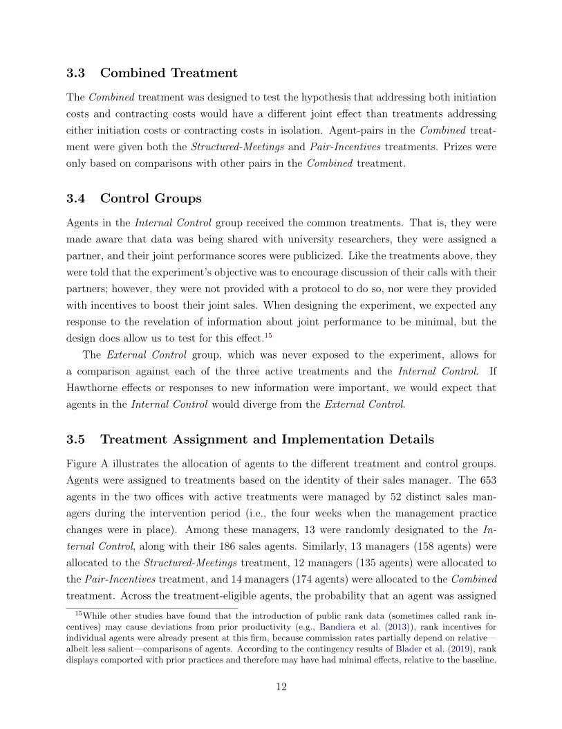
Figure A illustrates the allocation of agents to the different treatment and control groups.
Agents were assigned to treatments based on the identity of their sales manager. The 653
agents in the two offices with active treatments were managed by 52 distinct sales man-
agers during the intervention period (i.e., the four weeks when the management practice
changes were in place). Among these managers, 13 were randomly designated to the In-
ternal Control, along with their 186 sales agents. Similarly, 13 managers (158 agents) were
allocated to the Structured-Meetings treatment, 12 managers (135 agents) were allocated to
the Pair-Incentives treatment, and 14 managers (174 agents) were allocated to the Combined
treatment. Across the treatment-eligible agents, the probability that an agent was assigned
15While other studies have found that the introduction of public rank data (sometimes called rank in-centives) may cause deviations from prior productivity (e.g., Bandiera et al. (2013)), rank incentives forindividual agents were already present at this firm, because commission rates partially depend on relative—albeit less salient—comparisons of agents. According to the contingency results of Blader et al. (2019), rankdisplays comported with prior practices and therefore may have had minimal effects, relative to the baseline.
12

a partner reporting to his or her own manager was 0.40 each week, which ranged from 0.36
in the Pair-Incentives treatment to 0.47 in the Combined treatment. The External Control
group in the distant office contained 83 agents supervised by six managers. As part of the
design, movement between managers was restricted during the intervention period, and no
agents switched managers during these four weeks.16
Table 1 splits demographics and performance information by treatment assignment. The
agents in the three active treatment groups and the Internal Control group do not differ
based on pre-intervention sales productivity or demographic characteristics. That is, treat-
ment assignment is balanced across observables for treatment-eligible agents. P-values of
randomization tests of mean differences in the Internal Control and active treatment groups
are reported in the last column.17 Although the External Control group had lower average
sales per agent, sales trends in the External Control tracked those in the Internal Control
and the three active treatments prior to the experiment. Section 4.1 discusses parallel trends
tests prior to the intervention. We also test for balance across managers, the unit of ran-
domization. Across treatment arms, managers are similar in age, tenure, gender, and in the
average productivity of the agents they oversee. These manager-level averages, along with
the p-values of randomization tests of differences in means, are displayed by treatment in
Table A.2. During the intervention period, the average number of agents reporting to a
manager is balanced across treatments.
To communicate treatment assignment and intervention guidelines, senior executives
shared the details of the appropriate treatment with sales managers and support person-
nel, as they would be agents’ first resource if they had questions. Managers and support
personnel were told that the research staff would be allocating agents to different treatments
in order “to better understand and improve [agent] motivation, [agent] retention, and ulti-
mately, [agent] satisfaction.” Staff were told to communicate this to agents, if asked. Posters
around the office announced a “Sales Sprint” undertaken in conjunction with the help of
university researchers that would last four weeks. Agents were directed to a website that
explained their own treatment. (See Appendix B.2 for the text of communication.) Workers
were provided with a specific login key, based on their treatment assignment, so they could
only review details of their own treatment. Email and phone hotlines were established to
answer questions that were not directed to sales managers. Finally, a subset of the authors
16Agents typically switch managers on average between one to two times per year. After the interventionperiod, there was some reallocation of agents to other managers. Ninety-six agents had a different managerduring at least one week between weeks 5 and 10 (the six weeks following intervention), and 277 agents wereobserved with a different manager during at least one week in the 20 weeks following the interventions.
17These tests are computed from a regression of the variable of interest on treatment-assignment dummiesafter clustering standard errors, based on manager identity (the level of assignment). P-values are for thejoint test on these treatment-assignment dummies.
13

were on-site at least three days a week during the intervention period. Appendix B.1 provides
details about the sequence of steps used to implement the intervention.
Full Sample58 Managers(736 Agents)
Distant Office6 Managers(83 Agents)
No Randomization into TreatmentsNo Knowledge of the Experiment
No Pairings
External Control6 Managers(83 Agents)
Local Offices52 Managers(653 Agents)
Cluster Randomization into TreatmentsPaired with a Partner
Joint Performance Publicized
Internal Control13 Managers(186 Agents)
No AdditionalInstructions
Structured-Meetings13 Managers(158 Agents)
Self-ReflectiveWorksheets/Lunch
with Partner
Pair-Incentives12 Managers(135 Agents)
Competingfor Prizes
with Partner
Combined14 Managers(174 Agents)
Self-ReflectiveWorksheets/Lunch
& Competingwith Partner
Figure A: Allocation of Agents to Treatments
14

4 Results Identified by the Experiment
This section presents evidence on treatment effects during the four weeks with active in-
terventions and how these effects persist into the post-intervention period. Figure 2 shows
average revenue-per-call (RPC) gains during the intervention period in all three active treat-
ment groups.18 Beginning with a pre-intervention baseline of $61, RPC increased by $11
for agents in the Pair-Incentives treatment, whereas the Structured-Meetings and Combined
treatments yielded an RPC increase of approximately $15 relative to the pre-intervention
mean. RPC did not change for agents in the Internal and External control groups. Figure 3
shows RPC by week for each treatment group. Positive effects were present for all three active
treatments in week one (the first week of the intervention) and remained positive for the rest
of the intervention period. Beyond week four, when interventions ended, RPC remained ele-
vated for agents in the Structured-Meetings and Combined treatments. In contrast, average
RPC immediately collapsed to the control mean for agents in the Pair-Incentives treatment.
The sales increases in weeks one through four were likely achieved through different chan-
nels. If knowledge was exchanged, then any associated productivity gains should persist. The
experiment was intentionally designed to measure such persistence in the post-intervention
period. Agents who were provided a protocol through which to exchange contextual knowl-
edge with their partners in the Structured-Meetings and Combined treatments persistently
increased their sales, likely by applying this new knowledge. The Pair-Incentives treatment,
on the other hand, likely induced only transitory increases in effort. Supporting this in-
terpretation, we show that treatment effects on sales are largest where knowledge exchange
is most likely: for agents paired with high-performing partners and agents who document
contextual knowledge on their worksheets.
4.1 Estimation and Inference with Difference-in-Differences
Our empirical strategy uses difference-in-differences, which 1) enables comparisons relative to
the External Control, an office with lower levels of pre-experiment sales productivity than the
treatment-eligible agents, and 2) increases power for analysis of heterogeneous responses by
reducing the influence of between-subject or between-manager variability. Figure 3 provides
support for this approach by showing similar pre-intervention trends across groups.19 The
18To facilitate comparisons of changes across groups, Figure 2 displays RPC normalized to the grand-mean in the week prior to the intervention period (week 0) for the active treatment groups. Table 1 presentsnon-normalized summary statistics, averaged across agents, in the pre-intervention period.
19To formally test for pre-trend differences, we interact time indicators and treatment indicators in thepre-intervention period. We test for pre-trends using both four and eight weeks of pre-intervention data.After regressing log RPC on these time-by-treatment indicators in the pre-intervention period, we fail toreject that any are statistically different from zero at the 10% level (the smallest p-value is 0.48).
15
main estimating equation is:
Yi,t =β0 + β1Structured-Meetingsi x Tt + β2Pair-Incentivesi x Tt (1)
+ β3Combinedi x Tt + β4Internal-Controli x Tt + λt + θg + εi,t,
where Yi,t is a dependent variable of interest, i represents an agent, t represents a week,
g represents a sales manager group, λt and θg are week and sales manager fixed effects,
respectively, and εi,t is an idiosyncratic error term. The level effects of each treatment are
subsumed by the sales manager fixed effects, because all agents reporting to a sales manager
are assigned to the same treatment. Week fixed effects remove common time shocks that
affect all workers. The indicator Tt is a placeholder for either the intervention period or the
post-intervention period, indicating that interventions were either occurring or had occurred
in the past. For example, when the sample includes the pre-intervention period (weeks -3 to
0) and the intervention period (weeks 1 to 4), the variable Structured-Meetingsi x Tt is set
to one during weeks 1 to 4 for those agents randomly assigned to the Structured-Meetings
treatment and to zero otherwise. When the sample consists of the pre-intervention period
and the post-intervention period (weeks 5 to 24), the variable Structured-Meetingsi x Tt is
set to one during weeks 5 to 24.
Standard errors are clustered at the manager level, the unit of treatment assignment.
We also use randomization inference to compute exact p-values for the null of no treatment
effects, as described by Young (2018). Subsequent tables present p-values of joint hypothesis
tests of no significant treatment effects after accounting for clustered treatment assignment
by manager and re-randomizing treatments across managers.
4.2 Treatment Effects on Log Revenue-per-Call During the Inter-
vention Period
Table 2 presents treatment effects for log revenue-per-call during the intervention period.20
The sample contains the four weeks of data in the pre-intervention period and the four weeks
of data during the intervention period. Consistent with the graphical evidence, the active
treatments resulted in large, statistically significant increases in sales. Randomization tests
reject the joint null of no treatment effects for the three active treatments at the 1% level
in all columns. Point estimates on log RPC range from 0.22 to 0.25 for Structured-Meetings.
They are positive but smaller for Pair-Incentives, with point estimates between 0.13 and 0.14.
20Skewness in the distribution of sales naturally motivates using a log transformation for revenue. Wereport estimates below that demonstrate the results are not sensitive to levels, logs, or alternate performancemeasures.
16

Wald tests at the bottom of the table reject equality of sales gains in the Structured-Meetings
and Pair-Incentives treatments. Treatment effects for the Combined group are very similar
to those for agents with Structured-Meetings alone, indicating that the additional benefit
of addressing contracting costs was relatively small. In the final row, most specifications
reject the hypothesis that the Combined treatment effect is greater than the sum of the
individual Structured-Meetings and Pair-Incentives effects. That the incremental effect of
adding the Pair-Incentives in addition to Structured-Meetings is smaller than the baseline
effect of Pair-Incentives alone may indicate crowd out of monetary incentives or reduced
salience of the incentives when presented in conjunction with the instructions surrounding
the Structured-Meetings treatment.
The results are stable across different control groups. The specification in Column 1 is
relative to the Internal Control (so β4 in equation 1 is omitted); Column 2 replaces the
Internal Control group with the External Control as the baseline. Columns 3 and 4 add
back the Internal Control. Estimates change little across columns. Agents in the Internal
Control were aware of the experiment (see Appendix Table A.1, Panel B), had an assigned
partner, and had publicized joint sales information, but they did not change their sales,
relative to the (off-site) External Control group that was unaware of the experiment. The
sales increases in the active treatments are thus unlikely to be driven by Hawthorne effects or
by the common treatments across groups. Merely displaying performance information was
not sufficient to improve sales, likely because most agents were already aware of their place
in the distribution (see Online Appendix Figure OA.2). These estimated treatment effects
are robust to the inclusion of agent fixed effects in Column 4 and are not due to differential
turnover (discussed in Section 5.2).
The results from the intervention period point to the efficacy of treatments. Providing
group-based incentives increased output, as in Friebel et al. (2017) and Bandiera et al. (2013).
In addition, the Structured-Meetings treatment, meant to reduce initiation costs, resulted in
larger sales increases than the Pair-Incentives treatment alone. This larger increase becomes
apparent graphically in weeks 2 through 4 in Figure 3, as the effects of the Pair-Incentives
treatment appear to decline relative to the immediate spike in the first week. While we cannot
reject a uniform effect across weeks 1 to 4 in the Pair-Incentives treatment, average RPC
does coincide with agents’ pre-experiment reported valuations for the prizes each week.21
21The average cost of the prizes was about $50 each week. When surveyed about the value of eachprize prior to the experiment, average valuations for the prizes week by week were $46, $37, $36, and $40,respectively. A back-of-the-envelope calculation suggests that if an incentive with subjective value of $40resulted in a 0.14 unit increase in log RPC relative to the control group during the intervention period, thento achieve the same 0.24 unit increase realized by agents in the Structured-Meetings treatment observed inTable 2, the incentives would need to have a subjective value in excess of $69 ≈ (0.24× $40)/0.14.
17

Any decline week to week in the Pair-Incentives treatment is minimally driven by agents
becoming satiated after winning or discouraged after failing to win a prize. (See Table OA.1
in the Online Appendix).
These estimates provide some guidance for how output might respond when practice
changes permanently remain in place. Following Athey and Stern (1998) and Ichniowski and
Shaw (2003), the final row in Table 2 provides a test of whether the Structured-Meetings
and Pair-Incentives treatments should be implemented together. These results indicate
that the Structured-Meetings and Pair-Incentives treatments are substitutes, implying that
evaluating whether to bundle the practices depends on the marginal benefit of the Combined
treatment.22 Using the results for log RPC, the Combined treatment increased sales by
about 1% per call in addition to the Structured-Meetings effect, increasing revenue by about
$40 per week for each agent. Given that the per-agent cost of the Pair-Incentives treatment
was about $17 per week, the marginal gain from adding incentives appears to outweigh
the incremental cost, but the results fall within the confidence intervals for the Structured-
Meetings effect size in isolation. To understand the mechanism behind the treatments, we
turn to their persistence in the post-intervention period.
4.3 Persistence of Treatment Effects in the Post-Intervention Pe-
riod
To assess persistence of the observed sales gains, we re-estimate equation (1) with the four
weeks of pre-intervention data and the post-intervention period, weeks 5 through 24. The
results, reported in Table 3, are consistent with Figure 3 on the time series averages of RPC
by treatment. Treatments addressing initiation costs lead to persistent gains. Agents in
the Structured-Meetings treatment have log RPC that is 0.17 to 0.21 greater than agents in
either control group, representing persistent sales gains between 18% and 23%. The Com-
bined treatment also had positive gains in excess of 20% after interventions ended. Using
randomization inference, the joint test of no persistent treatment effect for the three active
treatments rejects the null at the 5% level in all columns.23 Post-intervention sales gains for
the Pair-Incentives group are statistically indistinguishable from either control group. This
pattern of results points to different mechanisms behind the sales gains during the inter-
vention period. The transitory gains in Pair-Incentives treatment indicate temporary effort
increases, while the persistent gains in the Structured-Meetings and Combined treatments
22One possible reason the treatments are substitutes is crowdout of monetary incentives; see Benabou andTirole (2006), Ederer and Manso (2013), Frey and Oberholzer-Gee (1997), and Gneezy et al. (2011).
23 The standard errors resemble those obtained when using two-way clustering by sales manager and week.(See Table OA.2 in the Online Appendix.)
18

are consistent with knowledge transmission between agents.
Columns 1–3 of Table 3 are analogous to the corresponding columns in Table 2 but with
differing time periods. Comparing parameter estimates across tables indicates that about
80% of the initial sales gains in the Structured-Meetings and Combined treatments remain
after interventions end. We find substantial persistence in sales gains for these treatments
through the end of the post-intervention horizon, as detailed in Appendix Table A.3. Ex-
tended graphical evidence through 34 weeks in Figure OA.3 shows that treatment effects
remain persistent beyond the end of the sample. Given these large, persistent gains, we
attempted to validate them using “insider econometrics” approaches (Bartel et al., 2004).
This entailed interviews with sales, operations, and HR executives, where we asked about
the plausibility of effect sizes and the underlying mechanisms that may be responsible. These
managers reported that adopting new sales techniques or fixing regularly occurring problems
would provide agents with long-term gains. Management also observed that the Structured-
Meetings treatment provided a pathway for agents to continue asking questions and gaining
knowledge from their partners, even after the formal meetings and lunches ceased. They be-
lieved these follow-up interactions increased the likelihood that treated agents would sustain
their higher sales.
A different possibility is that long-run gains arise due to the attrition of agents, but
Columns 4 and 5 suggest that workforce composition changes are unlikely to be responsible
for the persistent sales gains. Column 4 tests for sensitivity to agent attrition by using a
balanced sample approach, where gains are estimated for the particular agents who remain
at the firm during the post-intervention period. The balanced sample of agents in Column 4
is restricted to those agents who are present in the intervention period and remain in the data
through at least week 19.24 The number of agents in the sample falls to 388 unique agents,
reflecting that 1) this is a high-turnover industry25 and, more importantly, 2) turnover is
seasonal. The experiment occurred immediately prior to a focal moving and back-to-school
period, which is the highest turnover time of year for similar firms in both the local sales and
call center industries. The estimated effects in the balanced sample are very similar to those
in Column 3. Column 5 returns to the baseline sample of all agents, adding individual worker
fixed effects. This specification provides an additional diagnostic that accounts for potential
correlation between baseline productivity and retention throughout the post-intervention
period. Like the results in Column 4, the specification with individual fixed effects is quite
similar to those with only manager fixed effects. These results point to large, persistent
24The word “balanced” is shorthand to reflect that these are agents who do not leave the sample, ratherthan to indicate that they are present in all weeks.
25 Figure 1 of Hoffman et al. (2017) indicates that workers in similar types of service-sector jobs have amedian completed tenure of about 100 days.
19

gains from treatment, rather than explanations based on worker sorting or the retention of
the best agents. A complementary exercise provides visibility into whether the gains are
driven by survivors who do not leave the firm by weighting the regressions by the inverse
of the number of observations an agent is observed in the sample. The results in Online
Appendix Table OA.3 show similar or slightly larger point estimates for the Structured-
Meetings treatment and point estimates that range from slightly smaller and less precise
(while remaining significant) to somewhat larger for the Combined treatment.
4.4 Other Output Measures During the Intervention and Post-
Intervention Periods
The main results are similar across revenue measures and are not sensitive to the level of
aggregation. (See Appendix Table A.4 for results that aggregate to the manager level.) Table
4 presents difference-in-differences estimates of equation (1), where odd-numbered columns
correspond to the analysis of changes during the intervention period and even-numbered
columns to changes in the post-intervention period. All three active treatments lead to
total revenue increases during the intervention period. In the post-intervention period, total
revenue is $817 higher than the controls in the Structured-Meetings treatment and $811
higher than the controls in the Combined treatment. These increases in total revenue suggest
that gains did not come at the expense of taking fewer calls or working fewer hours. The
Pair-Incentives point estimate is indistinguishable from zero in the post-intervention period.
The next six columns repeat the analysis for revenue-per-hour (RPH), log RPH, and RPC
in levels, all showing broadly similar results.26 Comparisons of RPH and RPC allow for the
possibility that RPC fails to account for time away from the phones while meeting with
a partner, which would be evident if the RPH treatment effects were substantially lower.
However, the Structured-Meetings treatment estimate of log revenue-per-hour is broadly
similar to the estimate for log revenue-per-call in Column 3 of Table 2 for the intervention
period. Effects sizes are slightly smaller for the Pair-Incentives and Combined treatments,
relative to their log RPC analogs. Log revenue-per-hour remains 14 log points higher than
the control groups for the Structured-Meetings treatment in the post-intervention period and
is 16 log points higher for the Combined treatment. The results for RPC in Columns 7 and
8 show broadly similar patterns to the estimates using log RPC as the dependent variable.
A final question is whether any gains came at the expense of quality, a dimension that is
26Estimated effects on total revenue in the post-intervention period are larger than in the interventionperiod, yet RPC and RPH effects in the post-intervention period are no greater than in the interventionperiod. This indicates that some of the gain in total revenue in the post-intervention period is likely due toincreases in total hours spent working.
20

harder to observe. In other settings, it may be possible to increase revenue or profits through
reduced service quality, but that is less of a concern here. There are no repeat interactions
with customers, so the net revenue metrics mostly capture any effects of service quality
deterioration. Upstream brand providers also perform call audits to ensure that sales agents
accurately represent their products, but we do not have access to that data. However, as
mentioned earlier, agents’ commissions include a quality multiplier based on these audited
scores. With the commission data we have available, we construct a proxy for quality by
considering how agents’ commissions, relative to revenue, vary with treatment. Appendix
Table A.5 provides additional details and estimation results. We generally find no changes
in this quality proxy. Conversations with managers did not surface concerns about quality
reductions.
4.5 Sales Changes by Partner Performance
To further explore the mechanism, we leverage random agent pairings with high-performing
partners to assess how partner (pre-intervention) performance affects treatment gains. For
this analysis, we create a binary classification, sorting agents based on their sales productiv-
ity preceding the intervention. Agents are labeled “high-performers” if their productivity is
above the median in the eight weeks prior to the intervention for their division; agents who
join the firm during the intervention period are assumed to be low performers. (RPC for
these agents is significantly below the median.) Figure 4 plots average RPC by treatment
group and partner identity during the intervention and post-intervention periods. Aver-
age RPC is unaffected by partner quality in the Internal Control and the Pair-Incentives
treatments. In both the Structured-Meetings and Combined treatments, agents matched
with high-performing partners have higher average RPC than agents matched with low-
performing partners. Differences by partner quality remain in the post-intervention period,
indicating that both concurrent and persistent gains are larger when agents are randomly
matched with a more productive partner.
In line with the results in the theoretical appendix, we expect productivity gains to be
largest for agents paired with high-performers if treatment induces contextual knowledge
exchange that can be applied by others. We also expect this productivity gain to be larger
for low-performers when paired with high-performers, compared to high-performers when
paired with other high-performers. To estimate these effects, we interact partner quality
21

with treatment in the following equation:
Yi,t = β0 + β1Structured-Meetingsi x Tt + β2Pair-Incentivesi x Tt (2)
+β3Combinedi x Tt + γ1Structured-Meetingsi x Tt x High-Performing Partnert
+γ2Pair-Incentivesi x Tt x High-Performing Partnert
+γ3Combinedi x Tt x High-Performing-Partnert + γ4Tt x High-Performing Partnert
+γ5Ever High-Performing Partneri + λt + θg + εi,t,
where the variable Tt is again a placeholder to indicate either the intervention period or
the post-intervention period. The parameters of interest are γ1, γ2, and γ3, comparing how
high-performing partners affect sales productivity in different treatments. The parameter γ4
captures the baseline effect of having a high-performing partner for agents in the Internal
Control group. The parameter γ5 allows for differences in the pre-intervention period that
may be correlated with the propensity to match with a high-performing partner subsequently
(Guryan et al., 2009). This analysis omits the External Control group, as these agents did
not have partner assignments. We conduct the analysis where the dependent variable is
RPC in levels, as it allows for assessment of the optimal assignment rule between high- and
low-performers.27
Table 5 shows that agents randomly paired with a high-performing partner in the Structured-
Meetings and Combined treatments had larger gains in RPC than did other agents during
both the intervention and post-intervention periods. Agents paired with a high-performing
partner during the intervention weeks increased revenue-per-call by an additional $10.89 in
the Structured-Meetings treatment over the baseline Structured-Meetings treatment effect of
$11.94 (Column 1).28 High-performing partners in the Combined treatment raised average
RPC by $15.87 on top of the baseline treatment effect of $7.51. Agents in the Pair-Incentives
treatment did not have a statistically significant improvement on top of the baseline treat-
ment effect of $8.68 when they were paired with a high-performing partner. The last row
of the table presents results from tests of the joint null that there are no heterogeneous
effects by partner quality in the Structured-Meetings, Pair-Incentives, and Combined treat-
ments. These tests come from wild cluster bootstrapping while imposing the null hypothesis
(Roodman et al., 2019). We use this procedure as an alternative to randomization inference
because the assignment of high- and low-performing partners happens at a level below the
27The analysis in logs is reported in Table OA.4 in the Online Appendix and provides qualitatively similarconclusions.
28In the columns corresponding to the intervention period, high-performing partners are defined based onthe concurrent identity of the partner; i.e., the High-Performing-Partner dummy variable is applied at theagent-week level for those agents who rotated partners each week.
22

clustered unit of randomization.
The gains from being matched with a high-performing partner are largest for low-performing
agents. Columns 2 and 3 split the sample depending on whether the agent is himself or herself
a high-performer. Comparing these columns, all low-performing agents in active treatments
benefited, even when paired with low-performing partners (baseline estimates in Column 2).
When paired with a high-performing partner, captured through the interaction terms in Col-
umn 2, low-performing agents had additional positive gains in the Structured-Meetings and
Combined treatments of $17.25 and $21.55, respectively. When the agent himself or herself is
a high-performer (Column 3), we can reject a zero effect only when they are partnered with
another high-performing agent in the Structured-Meetings or Combined treatments.29 Said
another way, we are unable to detect sales gains in any treatment for high-performing agents
when they are paired with low-performing partners. Importantly, high-performers them-
selves did not see a decrease in RPC during treatment, suggesting that their performance on
calls was not harmed by the interventions. To further probe whether meetings came at the
expense of sales, we also estimate equation (2), where the dependent variable is total calls
per week. Table OA.5 in the Online Appendix shows that there are no significant differences
in calls answered across treatments during the intervention period. This is true regardless of
agents’ pre-intervention performance and their partner assignments. That high-performers
do not change their total calls even when matched with low-performers indicates that time
spent conversing with other agents did not detract from selling opportunities.
Column 4 of Table 5 examines the persistence of high-performer effects in the post-
intervention period. Most of the long-run sales increases from the Structured-Meetings and
Combined treatments arise from agents who in the past were paired with a high-performer.
Columns 5 and 6 again split the sample based on the agent’s own baseline classification, show-
ing that persistent effects are greatest for low-performers who were previously paired with
high-performing partners. Although having a high-performing partner benefits all agents,
the larger interaction terms in Columns 2 and 5 compared to Columns 3 and 6 indicate that
low-performers benefit most from matching with high-performers.
These results highlight the role of initiation costs as a limiting factor to knowledge ex-
change and, hence, productivity growth. Worksheets in the Structured-Meetings and Com-
bined treatments directed individual agents to reflect on their own recent sales strengths and
weaknesses before directing a similar set of questions to their partners in face-to-face meet-
ings. Neither the self-reflection exercise nor the (potentially) improved ability to formulate
or articulate requests for help can fully explain the differing treatment effects across agents
29For the Pair-Incentives treatment, no heterogeneous responses by partner quality are present whensplitting the analysis by low- and high-performer agents.
23

matched with high-performing partners, and those matched with low-performing partners.
This is because agents paired with low-performers could have decided themselves to reach
out for help from high-performers; i.e., absent initiation costs, there was nothing preventing
agents from using the worksheets in an unofficial capacity. Section 5.1.2 discusses what can
be said about the sources of these initiation costs in more detail.
4.6 Sales Dispersion in the Post-Intervention Period
The evidence that low-performers have the largest gains from treatments suggests that the
experiment reduced sales dispersion. To examine this, Figure 5 plots the density of log RPC
in weeks 5 to 24 for the Internal Control and for the Structured-Meetings and Combined treat-
ments. The standard deviation of log RPC actually increases between the pre-intervention
and post-intervention periods for agents in the Internal Control group, moving from 0.50
to 0.55, consistent with productivity becoming more dispersed over time. In contrast, the
standard deviation of log RPC falls for agents in the Structured Meetings and Combined
treatments. The standard deviation of log RPC for the Structured-Meetings and Combined
treatments is 0.49 in the pre-intervention period and 0.40 in the post-intervention period.
For the Structured-Meetings and Combined treatments, Levene and Brown-Forsythe tests
reject the null of equal variances in the post-intervention period against the Internal Control
group, both in isolation and when the Pair-Incentives treatment is included.
A related question is how the assignment of high- and low-performing partners changed
the baseline gap in RPC between high- and low-performers. Prior to the intervention, low-
performers in the Structured-Meetings and Combined treatments had an average RPC of
$43.31, whereas high-performers had an average RPC of $69.74. Said differently, there was an
average gap between high- and low-performers of $26.43 per call. Returning to the estimates
in Table 5, Column 5, the sales lift to a low-performer from having a high-performing partner
is $21.55 compared to a sales lift of $7.89 from having a low-performing partner.30 Under
these estimates, assigning high-performers to low-performers closed 82% of the initial $26.43
gap in RPC, whereas pairing low-performers with each other closed 30% of the initial RPC
gap. The comparable numbers for high-performers can be found in Column 6, where the
sales lift associated with high- and low-performing partners are $7.69 and -$1.18, respectively.
Using these numbers, we evaluate how an assignment rule that rotates high-performers across
all agents would influence the gap between ex-ante high- and low-performers. We focus on
this rule because subsequent results suggest that rotating between partners, after at least
one week of being paired with a high-performer, has a statistically insignificant interaction
30Calculations for the effect of high-performers includes the High-Performer × Post interaction, which is-5.66 (standard error = 3.38) in Column 5.
24

effect on post-intervention sales. Under this rule, the gap between high- and low-performers
would be $12.57 in revenue-per-call, significantly lower than the initial gap in performance
absent the intervention.31
5 Additional Evidence and Discussion
This section provides additional evidence on the mechanism, considers alternative explana-
tions, and discusses the generalizability of our findings.
5.1 Evidence on the Mechanism
5.1.1 Knowledge Exchange in Worksheet Content
Agents in the Structured-Meetings and Combined treatments largely complied with the in-
structions to meet and fill out the worksheets, as over 80% of agents completed a worksheet
every week (see Appendix Table A.1). The worksheets provide a partial record from which
we can extract proxies for the content of conversations. We note that agent-pairs likely did
not record everything shared in their conversations, meaning that the worksheet content is
incomplete. Still, the worksheets capture instances of contextual knowledge being transferred
between agents. The most relevant worksheet field was the prompt “Please write down one
thing your partner recommended you to try.” Of the 497 completed worksheets, 390
included entries to this prompt.32
Two clear types of responses emerge. First, and most prevalent, is contextual knowledge
useful for the sales process. The knowledge exchanged largely consists of changes that agents
could implement on calls. Examples include advice to use a pre-recorded list of questions
on the computer notepad while transcribing customer responses; and to quote prices that
include add-ons rather than giving an itemized breakdown; to wait before offering discounts
until the caller reveals their needs; to quote full, higher prices first and then highlight the
value of sign-up specials. The second type of response consists of supportive comments and
encouragement. A third type is other content, which is neither knowledge nor support.
31Evaluating alternative assignment rules is more challenging, especially those that do not involve managerschoosing assignments. Although Hamilton et al. (2003) show, in the context of team formation in a garmentproduction facility, that high performers have positive spillovers and are willing to team with others, theextent that they would choose the right allocation in the absence of managerial intervention is an openquestion.
32Fewer worksheets were collected than the reported completion rates would indicate. Worksheets werehanded into sales managers and then collected by the support personnel before being returned to the authors.It is likely that some worksheets were completed but were never officially recorded.
25

Two approaches were used to classify worksheet content for analysis. The first, which
we label the word presence classification, associates key words or phrases with either knowl-
edge/advice/techniques, support/encouragement, or both.33 In the second approach, which
we label the blinded classification, we used a third-party student research assistant to cate-
gorize responses. This student was not aware of the purpose of the work, only that we were
studying whether salespeople converse with each other about knowledge to improve the sales
process or provide support or encouragement. There is high agreement between classification
schemes.
The word presence classification scheme involved parsing the 30 most prevalent non-stop
words from the worksheet text entries to classify the types of responses recorded. Responses
that do not include one of these 30 most prevalent non-stop words are initially categorized
as “other.” Table A.6 lists these words, along with examples, and displays the response type,
either knowledge or support.34 This classification approach labels 282 responses (72%) as
conveying knowledge, 60 responses as providing support, 26 responses as communicating
both, and 74 responses as “other.” We augmented this approach by manually inspecting
text entries that lacked any word used in the main classification scheme.35 After manual
classifications, 80% of all completed worksheets included evidence of contextual knowledge
exchange between partners. The blinded classification yields slightly more entries as contain-
ing contextual knowledge (322, compared to 310) and fewer entries as containing support (78,
compared to 92). Eighty-six percent of the classifications are identical, and 94% of entries
classified as containing contextual knowledge with the word presence scheme are classified
as containing contextual knowledge in the blinded review.
We use this data to assess whether knowledge transfer from the worksheet content is as-
sociated with post-intervention sales performance. We interact the dummy variable Received
Knowledge, which equals one if an agent’s worksheet is classified as conveying knowledge, and
33Many responses appear to be shorthand for a particular sequence of offers or product pitches, like “High-Quality Bundle 1 at $X price point, then Mid-Quality Bundle 2 and Additional Product A at $Y price point,”etc.
34The word “pitch,” or a response that is a dictation of an advised pitch, occurs the most often (N = 76),followed by the words “call,” “customer,” and “positive.” Twenty-four out of the 30 most prevalent wordsare attributed to conveying knowledge. These are: “pitch,” “call,” [product name], “customer,” “time,”“assume,” [brand name], “sell,” “process,” “push,” “ask,” “value,” “$”, “slow,” “phone,” “offer,” “control,”“hold,” “discover,” “rebuttal,” “price,” “close,” “quality,” and “connect.” The six words or phrases attributedto support are: “positive,” “confident,” “patience,” “breath,” “laugh,” and “don’t give up.”
35Most of these responses are clearly identifiable as either conveying knowledge or providing support. Ofthese 74 responses, 28 were classified as providing knowledge. Two examples of these responses are, “Haveall [of the] info right in front of you, [and] say it like a normal conversation” and “Try to find ways to solvethe problem if it’s a credit fail.” Of the remaining 46 responses, 32 were classified as providing support, withexamples including: “Don’t let the fear of striking out keep you from playing the game” and “[My] partneris new, he said I got it down.” After this second categorization procedure, 14 responses remained as “other.”
26

zero otherwise, with an indicator for the post-intervention period, Post-Period. The sample
is restricted to agents in the Structured-Meetings and Combined treatments for whom we
have at least one worksheet. We then estimate the following equation:
Yi,t = β0 + β1(Received Knowledgei x Post-Periodt) (3)
+β2(Received Knowledgei) + λt + θg + εi,t.
The base specification compares agents who received any knowledge to those who received
only support from their partner. Accordingly, the coefficient on Received Knowledge × Post-
Period in Column 1 of Table 6 can be interpreted as the persistent benefit to individual sales
performance from receiving knowledge. In Column 1, we restrict the sample to include only
worksheets that were codified using the 30 most prevalent non-stop words. In Columns 2 and
3, we incorporate the additional 60 worksheets that were manually inspected and categorized.
Column 3 allows content categorized as conveying both knowledge and providing support
to have a different effect from those providing knowledge alone. The small and insignificant
point estimate on Received Knowledge and Support × Post-Period suggests that there was
little benefit from receiving support in addition to knowledge. Column 3 also incorporates
agent fixed effects (omitting “received knowledge”), rather than manager fixed effects, and
the results remain similar. Column 4 changes the classification to use the blinded third-party
scheme, and the point estimates on Received Knowledge × Post-Period increase, relative to
the prior columns. Finally, Columns 5 and 6 use total revenue per week as the dependent
variable. The point estimates yield substantial effects on overall revenue for agents who
document knowledge exchange on their worksheets. These results indicate that knowledge
flows between workers occurred among agents in the Structured-Meetings and Combined
treatments. The large sales effects also suggest that it was knowledge transfers that drove
the increases in sales performance.
Note that this exercise of correlating worksheet responses with sales performance is ex-
ploratory, meant to illuminate the underlying mechanism. We are not attempting to identify
a causal relation between what agents wrote down and their future sales. Because the ma-
jority of worksheet responses show examples of knowledge exchange and this correlates with
subsequent sales, the evidence suggests that the most likely mechanism behind the experi-
mentally identified sales gains are knowledge spillovers, rather than explanations based on
agents’ improved sentiment or gains from agents reflecting upon the sales process. Link-
ing these results to effects by high-performing partners, 74% of low-performing partners
are classified as providing advice/knowledge on one or more worksheets, whereas 93% of
high-performing partners do so. The difference is significant at the 1% level, but we cannot
27
determine whether it arises because high-performers are more likely to provide knowledge, or
whether their partners are more likely to record the knowledge provided by high-performers.
5.1.2 Evidence on the Sources of Initiation Costs
Based on their commission rates, agents had been leaving, on average, about $35 to $43
per week on the table by not previously self-organizing to exchange knowledge with others.
What is it that stops agents from seeking out knowledge in the absence of explicit instructions
to do so? Survey evidence and auxiliary tests suggest that search costs and coordination
difficulties are unlikely to explain the results. Interview evidence points to social costs.
Search costs based on not knowing who to ask for advice, or failing to anticipate the
benefits of asking, appear small in this context. Agents know where they stand in the sales
distribution and can identify high-performers. Survey responses show that agents can identify
their relative standing compared to that of top-performing agents (see Figure OA.2 in the
Online Appendix) and 93% of survey respondents can name three agents in the top 10% of
the sales distribution for their division and location. Agents themselves estimate positive
treatment effects from asking others for help, suggesting they understand the benefits of
seeking out knowledge (see Figure OA.4 in the Online Appendix).
Proximity governs communication patterns between agents at baseline, but proxies for
social or physical distance do not yield differences in post-intervention sales gains. Twenty-
five percent of survey respondents report: “When I ask other agents for help, I always (100%
of the time) look for someone seated beside me.” Another 36% of agents report: “When I
ask other agents for help, I usually (greater than 75% of the time) look for someone seated
beside me.” If distance were the main impediment to knowledge exchange in this workplace,
we might expect those paired with partners on another team to have larger gains because
of the lower likelihood of redundant information coming from non-proximate individuals.
There is little evidence for this channel, as agents paired with those on different teams, who
are likely both physically and socially distant, have similar post-intervention gains to agents
paired exclusively with partners on their own teams. Each week, the probability that an
agent was matched with a partner on his or her own team was 0.4. Table OA.7 in the Online
Appendix fails to detect heterogeneous treatment effects in the post-intervention period for
agents matched with partners on different teams.36 This suggests that barriers to knowledge
36We also estimate heterogeneous effects in Online Appendix Table OA.6 based on whether the agent inquestion reported an above-median number of work-related conversations per week (5) prior to the beginningof the intervention period. The results show modestly larger effect sizes for agents who previously hadmore frequent work-related conversations in the Structured-Meetings and Combined treatments during theintervention period, but interaction effects are small in the post-intervention period. These results providefurther support for the notion that even agents who are more likely to know their partners or who already
28

exchange exist even for those who are co-located and familiar with one another.
The lack of evidence for search and coordination costs motivates an exploration of social-
based initiation costs. Interview evidence points in this direction, but the exact source of
social costs is difficult to identify and different forces may matter for some agents. Chan-
drasekhar et al. (2016) suggest that knowledge seekers may refrain from asking for help in
order to mitigate feelings of shame or to avoid sending negative signals about their type—
two potential social costs. Other agents report an intimidation factor to approaching others.
One sales agent in the Structured-Meetings treatment expressed her excitement to us when
she learned she had been paired with a very skilled coworker. Specifically, she said: “I
would never have had the courage to approach him for help or advice. But since we are
paired together for lunch, I get to learn from one of the best sales agents in the company!”
Collectively, the evidence suggests that the Structured-Meetings protocol enabled agents to
address knowledge gaps with others—something that even the well-connected among them
had previously failed to accomplish. Resolving the precise nature of the underlying social
cost(s), however, requires a more targeted research design, which falls outside the scope of
the present experiment.
5.2 Did Treatments Cause Changes in Retention?
The estimates with a balanced panel and with agent fixed effects in Table 3 suggest that
turnover differences were not responsible for the sales changes. The similarity of the estimates
suggests that the productivity gains are due to within-worker changes, rather than differential
turnover of unproductive agents across the different treatments. A more direct examination
of turnover shows that the propensity for agents to leave the sample did not change for those
in the Structured-Meetings or Combined treatments, relative to those in the Pair-Incentives
treatment or Internal Control group. These results are in Appendix Table A.7. We focus
on turnover among agents in the two offices that were aware of the experiment, as there are
seasonal differences in staffing across locations.37 Across the active treatments, there are no
statistically significant differences in agent turnover over any horizon, ranging from 8 to 24
weeks after the beginning of the interventions.
engage in work-related conversations with peers, benefited from the interventions.37In particular, locations with active treatments relied more heavily on seasonal hiring and had (pre-
dictably) higher natural attrition during the post-treatment period as summer was ending. There are,however, no differences in turnover between active treatments and the Internal Control group.
29

5.3 The Firm’s Return on Investment
The economic significance of the findings was apparent to the firm. The firm previously relied
exclusively on short-term, temporary boosts to monetary incentives to influence agents’ per-
formance. Controlled experiments of other practices, especially around knowledge sharing,
had not been conducted. Following the experiment (after week 34), the firm implemented a
mentoring program, where seasoned agents were partnered with new recruits, following the
protocols of the Structured-Meetings treatment.
To estimate total returns to the firm, we pool all of the data and estimate treatment effects
by week for total revenue. This has the advantage of allowing the estimates to vary based on
the agents who remain in each future period. Using these estimates, we conservatively adjust
for an 8% commission paid to agents, multiply by the number of agents, and discount future
revenue using a 12.5% annual rate. Through the 24 weeks in which we track sales, the present
value of revenue increases to the firm is $1.29 million for the Structured-Meetings treatment,
$1.14 million for the Combined treatment, and $457,000 for the Pair-Incentives treatment.
The per-treatment variable implementation costs (lunches, printed worksheets, prizes) were
under $15,000 for each treatment, with the lowest cost for the Structured-Meetings treatment.
These calculations do not include staff and academic overhead.
5.4 The Results in Context
How do the results compare with other studies on group incentives? Many studies find
positive effects, and one might have anticipated, following Englmaier et al. (2018), that
incentives would encourage leadership to foster knowledge transmission. The lack of per-
sistence in the Pair-Incentives treatment suggests that these incentives were insufficient to
overcome initiation costs. Because many group incentive studies occur in settings where
there is some degree of baseline goal alignment, these settings likely have somewhat lower
initiation barriers. Blader et al. (2019) emphasize that the effects of incentives, especially
those around competition, depend on whether the firm has a cooperative “relational con-
tract” with employees. In this firm, despite agent reports that others would provide help,
a factor contributing to initiation costs may be the perception of an individually oriented
workplace, driven by relative performance evaluation in pay and the firm’s tendency to cele-
brate individual achievement. An area for future work is to better understand the response
to joint incentives and how that response varies with firm culture. Still, the reluctance to
seek out knowledge is likely general to many environments, as recent evidence points to
widespread frictions around information sharing in other contexts. For example, Cullen and
Perez-Truglia (2018) quantify how frictions limit the spread of information that all cowork-
30

ers appear to value. In their setting, even when information is not considered sensitive and
rewards are offered for sharing, employees who are not connected (measured through overlap
at the firm) exhibit reluctance to approach one another for information.
Despite the ubiquity of production differences across workers in many industries, another
consideration is whether the results generalize beyond sales. Relative to many other indus-
tries, sales positions provide rapid feedback. Sales workers may avoid the costs of acquiring
job-specific knowledge until they gain information about their match with the job. Under
these dynamics, highly tenured agents would endogenously choose to acquire knowledge in
the absence of intervention, as their longer anticipated tenure with the firm would allow
them to spread initiation costs over many future transactions. To assess how this might
influence the estimates, we exclude the agents with the lowest quartile of tenure and re-
estimate treatment effects for more highly tenured agents. Point estimates in Table OA.8 for
the post-intervention period, excluding the lowest tenured agents, are greater than 80% of
the estimates for the full sample in the Structured-Meetings and Combined treatments; con-
fidence intervals always include the original estimates. This suggests that tenure and rapid
on-the-job feedback alone are unlikely to close the original performance gaps that motivated
the experiment.38
6 Conclusion
In many workplaces, output varies dramatically across individuals. Managers are quick to
credit workplace interactions—and their effort to stimulate such interactions—as a driving
force behind employee productivity. Economists might point to these interactions as one
reason that firms exist. Careful examination surfaces a host of economic questions. In
particular, what are the economic costs that limit peer knowledge flows in the workplace?
Two theorized frictions are contracting difficulties and initiation costs, with the latter defined
as barriers preventing one from seeking assistance. Contracting difficulties concern the lack
of incentives for others to share information, as highlighted in the team incentives literature
(Bandiera et al., 2013; Friebel et al., 2017). Initiation costs are less studied inside firms, but
adjacent literature suggests they may be important. In urban economics and the economics
of innovation, distance is one such barrier to finding information (Glaeser and Gottlieb,
2009; Glaeser et al., 1992; Catalini, 2017); search costs are another (Boudreau et al., 2017).
A newer literature studies the (micro) social frictions that may burden those seeking help
38A focal metric for the firm is the number of agents’ who make it past ninety days of tenure, as thisis the point where agents are thought to become full-performers. Our estimates include only agents withgreater than 88 days of tenure, suggesting that knowledge transfers were important sources of gains even forexperienced agents who had achieved the background productivity growth through on-the-job learning.
31

(Chandrasekhar et al., 2016).
Within firms, little evidence exists on the role of management practices to spark knowl-
edge sharing. Instead, the focus is largely on formal reporting practices or patterns of
delegation. To get at the importance of knowledge flows between coworkers, we ran a field
experiment that randomly paired more than 650 call center sales agents and then assigned
the pairs to treatments that addressed different frictions to knowledge flows. One treat-
ment, Structured-Meetings, targeted initiation costs by guiding randomly paired workers to
participate in structured, work-related conversations. A second treatment, Pair-Incentives,
targeted contracting frictions by tying together partners’ expected contemporaneous earn-
ings. A third treatment, Combined, simultaneously addressed both frictions.
Although all treatments raised contemporaneous individual sales, relative to the con-
trol groups, workers in the Structured-Meetings treatment had persistent performance gains,
while the performance gains from the Pair-Incentives treatment subsided at the end of the
intervention period. A number of additional results suggest that the management-led ap-
proach to breaking down initiation costs resulted in knowledge transfers from highly skilled
workers to less skilled ones. These findings add to a small but growing set of studies show-
ing that simple management interventions can dramatically raise productivity (Bloom and
Van Reenen, 2011; Bloom et al., 2013; Cai and Szeidl, 2017; Haynes et al., 2009; Englmaier
et al., 2018), while highlighting the role of social factors in the adoption of different practices
(Shue, 2013).
While our setting provides a nearly ideal environment for measuring the effects of coworker
knowledge spillovers, the managerial lessons for unlocking knowledge flows are more general
(Chandrasekhar et al., 2016). Many settings provide performance incentives and opportuni-
ties to interact with other individuals, such as classrooms, academic departments, or cities.
A fruitful area of future research surrounds how different matching protocols vary in their
propensity to facilitate knowledge flows between individuals.
32

References
Athey, Susan, Scott Stern. 1998. An empirical framework for testing theories about complementarityin organizational design. National Bureau of Economic Research Working Paper .
Bandiera, Oriana, Iwan Barankay, Imran Rasul. 2005. Social preferences and the response toincentives: Evidence from personnel data. The Quarterly Journal of Economics 120(3) 917–962.
Bandiera, Oriana, Iwan Barankay, Imran Rasul. 2007. Incentives for managers and inequalityamong workers: Evidence from a firm-level experiment. The Quarterly Journal of Economics122(2) 729–773.
Bandiera, Oriana, Iwan Barankay, Imran Rasul. 2010. Social incentives in the workplace. TheReview of Economic Studies 77(2) 417–458.
Bandiera, Oriana, Iwan Barankay, Imran Rasul. 2013. Team incentives: Evidence from a firm-levelexperiment. Journal of the European Economic Association 11(5) 1079–1114.
Barro, Robert J. 1991. Economic growth in a cross section of countries. The Quarterly Journal ofEconomics 106(2) 407–443.
Bartel, Ann, Casey Ichniowski, Kathryn Shaw. 2004. Using “insider econometrics” to study pro-ductivity. American Economic Review 94(2) 217–223.
Battiston, Diego, Jordi Blanes i Vidal, Tom Kirchmaier. 2017. Face-to-face communication inorganisations. Working Paper .
Becker, Gary S. 1962. Investment in human capital: A theoretical analysis. Journal of PoliticalEconomy 70(5, Part 2) 9–49. doi:10.1086/258724.
Benabou, Roland, Jean Tirole. 2006. Incentives and prosocial behavior. American Economic Review96(5) 1652–1678.
Blader, Steven, Claudine Gartenberg, Andrea Prat. 2019. The contingent effect of managementpractices. The Review of Economic Studies .
Bloom, Nicholas, Erik Brynjolfsson, Lucia Foster, Ron S. Jarmin, Megha Patnaik, Itay Saporta-Eksten, John Van Reenen. 2017. What drives differences in management? National Bureau ofEconomic Research, Working Paper 23300 .
Bloom, Nicholas, Benn Eifert, Aprajit Mahajan, David McKenzie, John Roberts. 2013. Doesmanagement matter? Evidence from India. The Quarterly Journal of Economics 128(1) 1–51.
Bloom, Nicholas, Raffaella Sadun, John Van Reenen. 2016. Management as a technology? NationalBureau of Economic Research, Working Paper 22327 .
Bloom, Nicholas, John Van Reenen. 2011. Human resource management and productivity. Handbookof Labor Economics 4 1697–1767.
Boudreau, Kevin J., Tom Brady, Ina Ganguli, Patrick Gaule, Eva Guinan, Anthony Hollenberg,Karim R. Lakhani. 2017. A field experiment on search costs and the formation of scientificcollaborations. Review of Economics and Statistics 99(4) 565–576.
33

Bursztyn, Leonardo, Robert Jensen. 2017. Social image and economic behavior in the field: Iden-tifying, understanding, and shaping social pressure. Annual Review of Economics 9 131–153.
Cai, Jing, Adam Szeidl. 2017. Interfirm relationships and business performance. The QuarterlyJournal of Economics 133(3) 1229–1282.
Carpenter, Jeffrey P., Glenn W. Harrison, John A. List. 2005. Field Experiments in Economics.Elsevier.
Carrell, Scott E., Bruce I. Sacerdote, James E. West. 2013. From natural variation to optimalpolicy? The importance of endogenous peer group formation. Econometrica 81(3) 855–882.
Catalini, Christian. 2017. Microgeography and the direction of inventive activity. ManagementScience 64(9).
Chan, Tat Y., Jia Li, Lamar Pierce. 2014. Compensation and peer effects in competing sales teams.Management Science 60(8) 1965–1984.
Chandar, Bharat K., Ali Hortacsu, John A. List, Ian Muir, Jeffrey M. Wooldridge. 2019. Designand analysis of cluster-randomized field experiments in panel data settings. National Bureau ofEconomic Research, Working Paper .
Chandrasekhar, Arun G., Benjamin Golub, He Yang. 2016. Signaling, stigma, and silence in sociallearning. Working Paper .
Conley, Timothy G., Christopher R. Udry. 2010. Learning about a new technology: Pineapple inGhana. American Economic Review 100(1) 35–69.
Cullen, Zoe B, Ricardo Perez-Truglia. 2018. The salary taboo: Privacy norms and the diffusion ofinformation. Tech. rep., National Bureau of Economic Research.
Ederer, Florian, Gustavo Manso. 2013. Is pay for performance detrimental to innovation? Man-agement Science 59(7) 1496–1513.
Edmondson, Amy. 1999. Psychological safety and learning behavior in work teams. AdministrativeScience Quarterly 44(2) 350–383.
Edmondson, Amy C., Zhike Lei. 2014. Psychological safety: The history, renaissance, and futureof an interpersonal construct. Annual Review of Organizational Psychology and OrganizationalBehavior 1(1) 23–43. doi:10.1146/annurev-orgpsych-031413-091305.
Englmaier, Florian, Stefan Grimm, David Schindler, Simeon Schudy. 2018. The Effect of Incentivesin Non-Routine Analytical Team Tasks—Evidence From a Field Experiment. Tech. Rep. 71.URL https://ideas.repec.org/p/rco/dpaper/71.html.
Frey, Bruno S., Felix Oberholzer-Gee. 1997. The cost of price incentives: An empirical analysis ofmotivation crowding-out. The American Economic Review 87(4) 746–755.
Friebel, Guido, Matthias Heinz, Miriam Kruger, Nikolay Zubanov. 2017. Team incentives andperformance: Evidence from a retail chain. American Economic Review 107(8) 2168–2203.
Fudenberg, Drew, Luis Rayo. 2017. Training and effort dynamics in apprenticeship. CEPR Dis-cussion Paper No. DP12126.
34

Garicano, Luis, Luis Rayo. 2017. Relational knowledge transfers. American Economic Review107(9) 2695–2730.
Garlick, Robert. 2014. Academic peer effects with different group assignment rules: Residentialtracking versus random assignment. Tech. rep., Mimeo, Duke.
Gibbons, Robert, Michael Waldman. 2004. Task-specific human capital. American EconomicReview 94(2) 203–207.
Glaeser, Edward L., Joshua D. Gottlieb. 2009. The wealth of cities: Agglomeration economies andspatial equilibrium in the united states. Journal of Economic Literature 47(4) 983–1028.
Glaeser, Edward L., Hedi D. Kallal, Jose A. Scheinkman, Andrei Shleifer. 1992. Growth in cities.Journal of Political Economy 100(6) 1126–1152.
Glaeser, Edward L., Bruce I. Sacerdote, Jose A. Scheinkman. 2003. The social multiplier. Journalof the European Economic Association 1(2-3) 345–353.
Gneezy, Uri, Stephan Meier, Pedro Rey-Biel. 2011. When and why incentives (don’t) work tomodify behavior. Journal of Economic Perspectives 25(4) 191–210.
Grant, Robert M. 1996. Toward a knowledge-based theory of the firm. Strategic ManagementJournal 17(S2) 109–122.
Guryan, Jonathan, Kory Kroft, Matthew J. Notowidigdo. 2009. Peer effects in the workplace:Evidence from random groupings in professional golf tournaments. American Economic Journal:Applied Economics 1(4) 34–68.
Hamilton, Barton H., Jack A. Nickerson, Hideo Owan. 2003. Team incentives and worker hetero-geneity: An empirical analysis of the impact of teams on productivity and participation. Journalof Political Economy 111(3) 465–497.
Hanna, Rema, Sendhil Mullainathan, Joshua Schwartzstein. 2014. Learning through noticing:Theory and evidence from a field experiment. The Quarterly Journal of Economics 129(3)1311–1353.
Hasan, Sharique, Rembrand Koning. 2017. Conversational peers and idea generation: Evidencefrom a field experiment. Harvard Business School Working Paper 17-101 .
Haynes, Alex B., Thomas G. Weiser, William R. Berry, Stuart R. Lipsitz, Abdel-Hadi S. Breizat,E. Patchen Dellinger, Teodoro Herbosa, Sudhir Joseph, Pascience L. Kibatala, Marie Carmela M.Lapitan, et al. 2009. A surgical safety checklist to reduce morbidity and mortality in a globalpopulation. New England Journal of Medicine 360(5) 491–499.
Hoffman, Mitchell, Lisa B. Kahn, Danielle Li. 2017. Discretion in hiring. The Quarterly Journalof Economics 133(2) 765–800.
Ichniowski, Casey, Kathryn Shaw. 2003. Beyond incentive pay: Insiders’ estimates of the value ofcomplementary human resource management practices. Journal of Economic Perspectives 17(1)155–180.
35

Jackson, C. Kirabo, Henry S. Schneider. 2015. Checklists and worker behavior: A field experiment.American Economic Journal: Applied Economics 7(4) 136–68.
Jacobs, Jane. 1969. The Economy of Cities. Vintage.
Katz, Lawrence F., Alan B. Krueger. 2019. Understanding trends in alternative work arrangementsin the United States. Tech. rep., National Bureau of Economic Research.
Lazear, Edward P. 2000. Performance pay and productivity. American Economic Review 90(5)1346–1361.
Lazear, Edward P., Kathryn L. Shaw, Christopher T. Stanton. 2015. The value of bosses. Journalof Labor Economics 33(4) 823–861.
Lo, Desmond, Wouter Dessein, Mrinal Ghosh, Francine Lafontaine. 2016. Price delegation andperformance pay: Evidence from industrial sales forces. The Journal of Law, Economics, andOrganization 32(3) 508–544.
Lyle, David S., John Z. Smith. 2014. The effect of high-performing mentors on junior officerpromotion in the US army. Journal of Labor Economics 32(2) 229–258.
Manski, Charles F. 1993. Identification of endogenous social effects: The reflection problem. TheReview of Economic Studies 60(3) 531–542.
Marshall, Alfred. 1890. Principles of Economics. London: Macmillan.
Mas, Alexandre, Enrico Moretti. 2009. Peers at work. American Economic Review 99(1) 112–45.
Morrison, Alan D., William J. Wilhelm Jr. 2004. Partnership firms, reputation, and human capital.American Economic Review 94(5) 1682–1692.
Myers, Christopher. 2015. Is your company encouraging employees to share what they know?Harvard Business Review 1–9.
Romer, Paul M. 1990. Endogenous technological change. Journal of Political Economy 98(5, Part2) S71–S102.
Roodman, David, Morten Ørregaard Nielsen, James G. MacKinnon, Matthew D. Webb. 2019. Fastand wild: Bootstrap inference in stata using boottest. The Stata Journal 19(1) 4–60.
Shue, Kelly. 2013. Executive networks and firm policies: Evidence from the random assignment ofMBA peers. The Review of Financial Studies 26(6) 1401–1442.
Young, Alwyn. 2018. Channeling fisher: Randomization tests and the statistical insignificance ofseemingly significant experimental results. The Quarterly Journal of Economics 134(2) 557–598.
36

Tables and Figures
Figure 1: Dispersion in Log Revenue-Per-Call
0.5
11.
5D
ensi
ty
2 3 4 5 6Log Revenue Per Call
Overall Due to Person Effects
This figure displays density plots of raw log revenue-per-call (Overall) and estimated log revenue-
per-call agent fixed effects (Due to Person Effects) using the eight weeks of data prior to the
intervention period. The sample includes 623 agents and 3,026 agent-weeks for those in the two
treatment-eligible offices. The sample does not include the 26 agents who joined during the in-
tervention period, nor does it include an additional four agents who moved from positions outside
of the six main sales divisions. The agent fixed effects come from a regression that nets out sales
division-by-week fixed effects, after which we apply the shrinkage procedure in Lazear et al. (2015).
The interquartile range and standard deviation of log RPC are 0.60 and 0.47, respectively. The
interquartile range and standard deviation of agent fixed effects are 0.39 and 0.30.
37

Figure 2: Mean Revenue-per-Call by Treatment Assignment During the Pre-Intervention and Intervention Periods
020
4060
80R
even
ue P
er C
all (
Nor
mal
ized
)
External Control Internal Control Pair Incentives Structured Meetings Combined
Pre-Intervention Intervention Period
This figure displays means of revenue-per-call (RPC) using four weeks of pre-intervention data and
four weeks of data during the intervention period (N=736 unique agents over 3,821 agent-weeks).
To facilitate visual comparisons of changes across time periods, data for each group are normalized
to the grand mean as of the week immediately prior to treatment (week 0), approximately $60 in
RPC. Table 1 provides additional detail on non-normalized revenue measures in the pre-period.
38
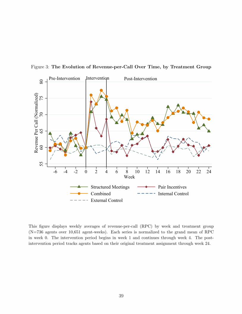
Figure 3: The Evolution of Revenue-per-Call Over Time, by Treatment Group
5560
6570
7580
Rev
enue
Per
Cal
l (N
orm
aliz
ed)
-6 -4 -2 0 2 4 6 8 10 12 14 16 18 20 22 24Week
Structured Meetings Pair IncentivesCombined Internal ControlExternal Control
Pre-Intervention Intervention Post-Intervention
This figure displays weekly averages of revenue-per-call (RPC) by week and treatment group
(N=736 agents over 10,651 agent-weeks). Each series is normalized to the grand mean of RPC
in week 0. The intervention period begins in week 1 and continues through week 4. The post-
intervention period tracks agents based on their original treatment assignment through week 24.
39

Figure 4: Average Revenue-per-Call in the Intervention and Post-InterventionPeriods by High-Performer Partner Assignment
020
4060
80R
even
ue P
er C
all
Internal Control Pair Incentives Structured Meetings Combined
Intervention Period, Low-Performer PartnerIntervention Period, High-Performer PartnerPost-Intervention, Low-Performer PartnerPost-Intervention, High-Performer Partner
This figure displays average revenue-per-call (RPC) by treatment group during the intervention
period (N=1,654 agent-weeks) and the post-intervention period (N=4,472 agent-weeks), based on
whether the agent was randomly paired with a high-performer (defined as above median RPC within
division in the pre-intervention period). Agents are classified as being paired with a high-performer
during the intervention period based on their concurrent partner match (N=833 agent-weeks with
a high-performer partner). In the post-intervention period, agents are classified as paired with a
high-performing partner if they were ever assigned a high-performer partner (N=2,896 agent-weeks
after pairing with a high-performer partner). The External Control group is not included in this
sample due to lack of a partner pairing.
40

Figure 5: Dispersion in Log Revenue-per-Call in the Post-Intervention Period
0.5
1D
ensi
ty
1 2 3 4 5 6Log RPC in Post Period
Meetings and Combined Internal Control
This figure displays log revenue-per-call density plots in the post-intervention period for agents
assigned to the Internal Control and the Structured-Meetings and Combined treatments (N=397
agents over 3,438 agent-weeks).
41
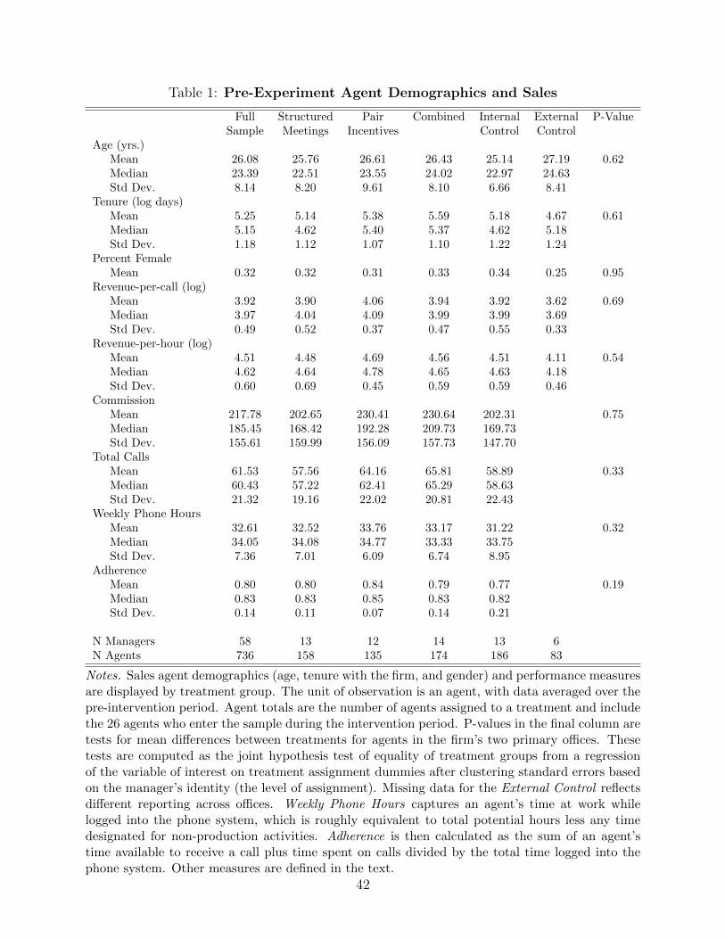
Table 1: Pre-Experiment Agent Demographics and Sales
Full Structured Pair Combined Internal External P-ValueSample Meetings Incentives Control Control
Age (yrs.)Mean 26.08 25.76 26.61 26.43 25.14 27.19 0.62Median 23.39 22.51 23.55 24.02 22.97 24.63Std Dev. 8.14 8.20 9.61 8.10 6.66 8.41
Tenure (log days)Mean 5.25 5.14 5.38 5.59 5.18 4.67 0.61Median 5.15 4.62 5.40 5.37 4.62 5.18Std Dev. 1.18 1.12 1.07 1.10 1.22 1.24
Percent FemaleMean 0.32 0.32 0.31 0.33 0.34 0.25 0.95
Revenue-per-call (log)Mean 3.92 3.90 4.06 3.94 3.92 3.62 0.69Median 3.97 4.04 4.09 3.99 3.99 3.69Std Dev. 0.49 0.52 0.37 0.47 0.55 0.33
Revenue-per-hour (log)Mean 4.51 4.48 4.69 4.56 4.51 4.11 0.54Median 4.62 4.64 4.78 4.65 4.63 4.18Std Dev. 0.60 0.69 0.45 0.59 0.59 0.46
CommissionMean 217.78 202.65 230.41 230.64 202.31 0.75Median 185.45 168.42 192.28 209.73 169.73Std Dev. 155.61 159.99 156.09 157.73 147.70
Total CallsMean 61.53 57.56 64.16 65.81 58.89 0.33Median 60.43 57.22 62.41 65.29 58.63Std Dev. 21.32 19.16 22.02 20.81 22.43
Weekly Phone HoursMean 32.61 32.52 33.76 33.17 31.22 0.32Median 34.05 34.08 34.77 33.33 33.75Std Dev. 7.36 7.01 6.09 6.74 8.95
AdherenceMean 0.80 0.80 0.84 0.79 0.77 0.19Median 0.83 0.83 0.85 0.83 0.82Std Dev. 0.14 0.11 0.07 0.14 0.21
N Managers 58 13 12 14 13 6N Agents 736 158 135 174 186 83
Notes. Sales agent demographics (age, tenure with the firm, and gender) and performance measuresare displayed by treatment group. The unit of observation is an agent, with data averaged over thepre-intervention period. Agent totals are the number of agents assigned to a treatment and includethe 26 agents who enter the sample during the intervention period. P-values in the final column aretests for mean differences between treatments for agents in the firm’s two primary offices. Thesetests are computed as the joint hypothesis test of equality of treatment groups from a regressionof the variable of interest on treatment assignment dummies after clustering standard errors basedon the manager’s identity (the level of assignment). Missing data for the External Control reflectsdifferent reporting across offices. Weekly Phone Hours captures an agent’s time at work whilelogged into the phone system, which is roughly equivalent to total potential hours less any timedesignated for non-production activities. Adherence is then calculated as the sum of an agent’stime available to receive a call plus time spent on calls divided by the total time logged into thephone system. Other measures are defined in the text.
42

Table 2: Log Revenue-per-Call Treatment Effects During the Intervention Period
Control Group: Internal External Both(Passive Pairs) (No Pairs)
(1) (2) (3) (4)
Structured-Meetings 0.241*** 0.247*** 0.247*** 0.224***(0.045) (0.044) (0.044) (0.065)
Pair-Incentives 0.131*** 0.141*** 0.140*** 0.126**(0.048) (0.046) (0.046) (0.061)
Combined 0.255*** 0.266*** 0.265*** 0.265***(0.043) (0.057) (0.057) (0.071)
Internal Control 0.010 0.058(0.044) (0.060)
Manager FE (θg) X X XIndividual FE (θi) XWeek FE (λt) X X X XAdj. R-Square 0.470 0.416 0.417 0.536Observations 3,418 2,856 3,821 3,821Individuals 653 550 736 736Managers 52 45 58 58P-Value from Randomization: <0.01 <0.01 <0.01 <0.01P-Values from Wald Tests:
H0: Meetings = Incent. 0.048 0.017 0.014 0.044H0: Meetings+Incent.≤Comb. 0.049 0.044 0.044 0.162
Notes. This table reports difference-in-differences estimates of treatment effects on log revenue-per-call using data from the four-week pre-intervention period and the four-week intervention period.The variables Structured-Meetings, Pair-Incentives, and Combined are shorthand for “Structured-Meetings x Intervention Period,” “Pair-Incentives x Intervention Period,” and “Combined x Inter-vention Period” and they are set to one in the intervention period for those randomly assigned tothose treatments, and zero otherwise. Dummy variables for treatment assignment in the pre-periodare absorbed by manager fixed effects, as randomization is at the sales manager level. In Column(1) the Internal Control (passive pairs) is the omitted category. Column (2) omits the InternalControl group and instead uses the External Control group (that was not aware of the experimentand had no partner pairing) as the excluded category. Other columns include both control groups,with an indicator for the Internal Control during the treatment period. The p-value from ran-domization tests reports the Young (2018) test of the sharp null of no treatment effects for thethree active treatments. The p-values from Wald tests in the bottom rows are tests of two nullhypotheses using the asymptotic covariance matrix: i) equality of effects between Pair-Incentivesand Structured-Meetings, and ii) the Combined group had sales gains that exceed the sum of thegains in the Structured-Meetings and Pair-Incentives groups. Standard errors are clustered at thesales manager level and are reported in parentheses. Statistical significance at the 10%, 5%, and1% levels is indicated by *, **, and ***, respectively, using the asymptotic covariance matrix.
43

Table 3: Log Revenue-per-Call Treatment Effects Post-Intervention
Control Group: Internal External Both(Passive Pairs) (No Pairs)
(1) (2) (3) (4) (5)
Structured-Meetings 0.189** 0.204** 0.204** 0.211** 0.174**(0.077) (0.084) (0.084) (0.085) (0.076)
Pair-Incentives 0.069 0.085 0.084 0.128 0.127(0.052) (0.070) (0.069) (0.087) (0.080)
Combined 0.210*** 0.225*** 0.225*** 0.231*** 0.276***(0.078) (0.080) (0.080) (0.081) (0.078)
Internal Control 0.017 0.038 0.063(0.076) (0.068) (0.063)
Manager FE (θg) X X X XBalanced panel XIndividual FE (θi) XWeek FE (λt) X X X X XAdj. R-Square 0.351 0.396 0.389 0.415 0.528Observations 6,236 6,026 7,334 5,518 7,334Individuals 628 535 711 388 711Managers 52 45 58 58 58P-Value from Randomization: 0.041 0.044 0.027 0.026 <0.01P-Values from Wald Tests:
H0: Meetings = Incent. 0.068 0.135 0.129 0.538 0.464H0: Meetings+Incent.≤Comb. 0.253 0.284 0.287 0.393 0.358
Notes. This table reports difference-in-differences estimates of persistent treatment effects on logrevenue-per-call using data from the four-week pre-intervention period and the 20-week post-intervention period (weeks 5-24). The variables Structured-Meetings, Pair-Incentives, and Com-bined are shorthand for “Structured-Meetings x Post-Intervention Period,” “Pair-Incentives x Post-Intervention Period,” and “Combined x Post-Intervention Period” and they are set to one in thepost-treatment period for those randomly assigned to those treatments, and zero otherwise. Salesmanager fixed effects correspond to the manager at the time of treatment assignment. Dummyvariables for treatments are absorbed by the individual or manager fixed effects. In Column (1) theInternal Control (passive pairs) is the omitted category. Column (2) omits the Internal Controlgroup and instead uses the External Control group (that was not aware of the experiment and hadno partner pairing) as the excluded category. Other columns include both control groups, with anindicator for the Internal Control during the post-treatment period. The balanced sample panelincludes only agents who remain in the data after week 19. The p-value from randomization reportsthe Young (2018) test of the sharp null of no treatment effects for the three active treatments. Thep-values from Wald tests in the bottom rows are tests of two null hypotheses using the asymptoticvariance-covariance matrix: i) equality of effects between Pair-Incentives and Structured-Meetings,and ii) the Combined group had sales gains that exceed the sum of the gains in the Structured-Meetings and Pair-Incentives groups. Standard errors are clustered at the sales manager level andare reported in parentheses. Statistical significance at the 10%, 5%, and 1% levels is indicated by*, **, and ***, respectively.
44
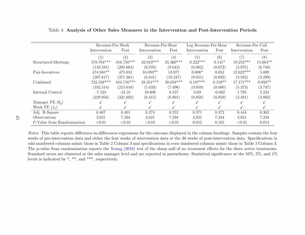
Table 4: Analysis of Other Sales Measures in the Intervention and Post-Intervention Periods
Revenue-Per-Week Revenue-Per-Hour Log Revenue-Per-Hour Revenue-Per-CallIntervention Post Intervention Post Intervention Post Intervention Post
(1) (2) (3) (4) (5) (6) (7) (8)Structured-Meetings 578.784*** 816.750*** 32.910*** 25.360*** 0.222*** 0.141* 19.252*** 15.664**
(143.585) (295.604) (6.876) (9.043) (0.082) (0.072) (3.975) (6.740)Pair-Incentives 474.945** 475.052 16.893** 13.977 0.086* 0.052 12.622*** 5.009
(207.817) (371.261) (6.841) (10.247) (0.051) (0.092) (3.582) (3.299)Combined 722.538*** 810.716*** 28.351*** 30.058*** 0.187*** 0.159** 17.171*** 9.950**
(182.514) (215.616) (5.433) (7.496) (0.059) (0.080) (5.373) (3.747)Internal Control -7.525 -21.21 10.606 8.557 0.03 -0.002 1.795 2.224
(229.956) (321.602) (6.415) (8.801) (0.058) (0.059) (2.491) (3.802)Manager FE (θg) X X X X X X X XWeek FE (λt) X X X X X X X XAdj. R-Square 0.467 0.401 0.274 0.252 0.371 0.372 0.444 0.362Observations 3,821 7,334 3,821 7,334 3,821 7,334 3,821 7,334P-Value from Randomization: <0.01 <0.01 <0.01 <0.01 0.012 0.165 <0.01 0.013
Notes. This table reports difference-in-differences regressions for the outcome displayed in the column headings. Samples contain the fourweeks of pre-intervention data and either the four weeks of intervention data or the 20 weeks of post-intervention data. Specifications inodd-numbered columns mimic those in Table 2 Column 3 and specifications in even numbered columns mimic those in Table 3 Column 3.The p-value from randomization reports the Young (2018) test of the sharp null of no treatment effects for the three active treatments.Standard errors are clustered at the sales manager level and are reported in parentheses. Statistical significance at the 10%, 5%, and 1%levels is indicated by *, **, and ***, respectively.
45
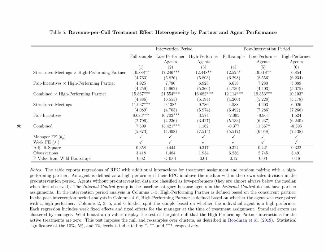
Table 5: Revenue-per-Call Treatment Effect Heterogeneity by Partner and Agent Performance
Intervention Period Post-Intervention Period
Full sample Low-Performer High-Performer Full sample Low-Performer High-PerformerAgents Agents Agents Agents
(1) (2) (3) (4) (5) (6)Structured-Meetings × High-Performing Partner 10.888** 17.246*** 12.448** 12.525* 19.318** 6.854
(4.763) (5.826) (5.803) (6.298) (8.556) (6.234)Pair-Incentives × High-Performing Partner 4.925 7.780 6.928 6.658 7.280 3.389
(4.259) (4.962) (5.366) (4.730) (4.403) (5.675)Combined × High-Performing Partner 15.867*** 21.554*** 16.682*** 12.114*** 19.353*** 10.103*
(4.886) (6.555) (5.194) (4.260) (5.228) (5.178)Structured-Meetings 11.937*** 9.138* 9.786 4.588 4.203 6.026
(4.089) (4.705) (5.974) (6.492) (7.286) (7.266)Pair-Incentives 8.683*** 16.702*** 3.574 -2.005 -0.964 1.524
(2.796) (4.236) (3.427) (5.133) (6.237) (6.240)Combined 7.509 15.421*** 1.162 -0.377 11.557* -8.395
(5.873) (4.498) (7.515) (5.517) (6.048) (7.138)Manager FE (θg) X X X X X XWeek FE (λt) X X X X X XAdj. R-Square 0.358 0.444 0.317 0.324 0.421 0.322Observations 3,418 1,484 1,934 6,236 2,745 3,491P-Value from Wild Bootstrap: 0.02 < 0.01 0.01 0.12 0.03 0.18
Notes. The table reports regressions of RPC with additional interactions for treatment assignment and random pairing with a high-performing partner. An agent is defined as a high-performer if their RPC is above the median within their own sales division in thepre-intervention period. Agents without pre-intervention data are classified as low-performers (they are almost always below the medianwhen first observed). The Internal Control group is the baseline category because agents in the External Control do not have partnerassignments. In the intervention period analysis in Columns 1–3, High-Performing Partner is defined based on the concurrent partner.In the post-intervention period analysis in Columns 4–6, High-Performing Partner is defined based on whether the agent was ever pairedwith a high-performer. Columns 2, 3, 5, and 6 further split the sample based on whether the individual agent is a high-performer.Each regression includes week fixed effects and fixed effects for the manager at the time of treatment assignment. Standard errors areclustered by manager. Wild bootstrap p-values display the test of the joint null that the High-Performing Partner interactions for theactive treatments are zero. This test imposes the null and re-samples over clusters, as described in Roodman et al. (2019). Statisticalsignificance at the 10%, 5%, and 1% levels is indicated by *, **, and ***, respectively.
46

Table 6: Post-Intervention Correlations Between Knowledge Documented inWorksheets and Sales
Log RPC Revenue
(1) (2) (3) (4) (5) (6)Received Knowledge × Post 0.169** 0.187** 0.168** 0.243*** 897.498*** 873.536**
(0.068) (0.074) (0.084) (0.056) (232.026) (202.090)Knowledge and Support × Post -0.053 0.044 -90.817 -82.712
(0.045) (0.051) (378.663) (136.455)Word presence classification XWord and manual classification X X XBlinded classification X XManager FE (θg) X X X X XIndividual FE (θi) XWeek FE (λt) X X X X X XAdj. R-Square 0.331 0.335 0.322 0.337 0.232 0.223
Observations 1,929 2,102 2,102 2,218 2,102 2,218
Notes. This table reports difference-in-differences estimates of log revenue-per-call and total rev-enue in the post-intervention period for agents in the Structured-Meetings and Combined treatmentsfor whom we have at least one completed worksheet. The reported coefficients represent the post-intervention change in the dependent variable for agents who received knowledge, or received knowl-edge and support, relative to agents who received supportive advice alone (the baseline). In Column1, these classifications come from the prevalence of the 30 most common words (excluding stop-words) as detailed in Table A.6. Columns 2, 3, and 5 include manually classified worksheet responsesbased on the authors’ readings. Columns 4 and 6 use classifications where a third-party studentwho was not briefed on the research was asked to classify some text snippets from from the work-sheets into categories. These categories were “The Statement Provides Knowledge/Advice/Tips toImprove Sales Performance,” “The Statement Provides Support,” “Both Knowledge and Support,”and “Other.” Eighty-six percent of the classifications between the Blinded 3rd party classificationsand the Word presence and Manual classifications align, while the Blinded 3rd party coding hasmore entries classified as “Received Knowledge.” Ninety-four percent of the entries classified as“Received Knowledge” in the Word presence and Manual scheme were also classified as “ReceivedKnowledge” in the Blinded 3rd party coding. Standard errors are clustered at the sales managerlevel and are reported in parentheses. Statistical significance at the 10%, 5%, and 1% levels isindicated by *, **, and ***, respectively.
47

Table A.1: Pre-Experiment and Post-Experiment Survey Responses for Treatment-Eligible Agents
Full Sample Internal Control Pair-Incentives Structured-Meetings Combined
Panel A: Pre-Experiment SurveyOn a scale of 1-5, how connected do you 3.7 3.7 3.4 3.7 3.8feel to others within the firm?
How many work-related interactions do you 5.8 5.0 5.3 7.1 6.1initiate in an average work week?
On a scale of 1-5, how beneficial are these 3.9 3.9 3.9 4.0 4.0interactions to you personally?
What dollar value would you be willing to $40.20spend on the proposed incentives?
Panel B: Post-Experiment Survey
I was aware of the [treatment] 82.5% 77.4% 78.3% 84.8% 92.0%that took place this past month.
We turned in a completed 82.6% 88.2%worksheet each week.
I spent [ ] minutes with my 6.3 7.3partner on the worksheet.
These interactions with my 78.6% 76.0%partner were beneficial.
NA (Agents) 378 115 83 105 75
Panel A contains answers from the preliminary survey that we administered one week prior to the start of the experiment. The surveywas not given to the External Control group. The question wording, as displayed, has been adapted from its original form to removeinstitutionally distinct jargon. Agents were provided with a link to the survey and were asked to complete it while at work. Agentswere not aware of which treatment they were going to be placed in at the time they took the survey. The question regarding the dollarvalue of the proposed incentives is the average valuation for the set of prizes offered in the Pair-Incentives treatment. Panel B containsresponses given at the end of the intervention period using the same protocol.
48

Table A.2: Balance Across Managers
Full Structured Pair Combined Internal External P-ValueSample Meetings Incentives Control Control
Manager Age (yrs.)Mean 29.27 29.38 29.15 28.97 30.62 27.02 0.853Std Dev. 4.972 4.336 4.209 6.269 5.775 2.085
Manager Tenure (yrs.)Mean 3.065 3.688 3.449 2.742 3.094 1.634 0.542Std Dev. 1.777 1.566 1.968 1.603 1.967 1.224
Manager FemaleMean 0.138 0.0769 0.167 0.0714 0.154 0.333 0.827Std Dev. 0.348 0.277 0.389 0.267 0.376 0.516
Average log(RPC) of Agentson Team Pre-Intervention
Mean 3.958 3.917 4.127 4.044 3.877 3.655 0.601Std Dev. 0.430 0.400 0.369 0.388 0.614 0.109
Number of Agents on Teamduring Intervention
Mean 12.69 12.15 11.25 12.43 14.31 13.83 0.870Std Dev. 4.07 3.60 3.68 3.06 4.40 3.13
N Managers 58 13 12 14 13 6
Notes. Manager demographics and average team characteristics are displayed by treatment group.P-values in the final column are tests for differences between groups for treatment-eligible agentsin the firm’s two primary offices. These tests are computed as the joint hypothesis test of equalityof treatment group indicators from a regression of the variable of interest on treatment assignmentdummies.
49

Table A.3: Estimates of Persistence of Log RPC Gains Over Different Intervalsin the Post-Intervention Period
Weeks Weeks Weeks Weeks Weeks Weeks5–8 9–12 13–16 17–20 21–24 5–24(1) (2) (3) (4) (5) (6)
Weeks 5–8Structured-Meetings 0.208*** 0.258***
(0.061) (0.077)Pair-Incentives 0.030 0.058
(0.057) (0.071)Combined 0.242*** 0.288***
(0.062) (0.084)Weeks 9–12Structured-Meetings 0.090 0.087
(0.075) (0.078)Pair-Incentives 0.039 0.019
(0.060) (0.063)Combined 0.147** 0.123
(0.071) (0.074)Weeks 13–16Structured-Meetings 0.176 0.185*
(0.108) (0.108)Pair-Incentives 0.044 0.076
(0.093) (0.094)Combined 0.144 0.142
(0.095) (0.096)Weeks 17–20Structured-Meetings 0.177 0.216
(0.140) (0.130)Pair-Incentives 0.064 0.140
(0.125) (0.116)Combined 0.231* 0.259**
(0.130) (0.119)Weeks 21–24Structured-Meetings 0.136 0.188*
(0.113) (0.105)Pair-Incentives 0.030 0.129
(0.096) (0.089)Combined 0.154 0.211**
(0.104) (0.096)Manager FE (θg) X X X X X XWeek FE (λt) X X X X X XAdj. R-Square 0.418 0.290 0.319 0.301 0.306 0.339Observations 3,252 2,724 2,545 2,426 2,341 6,236
This table presents estimates of log RPC persistence using a specification analogous to Table 3Column 1. Columns 1–5 include the pre-period and a different four-week interval in the post-intervention period. The variables Structured-Meetings, Pair-Incentives, and Combined are set toone in the weeks after the intervention for those assigned to the treatment and are zero otherwise.The specification in Column 6 includes separate interactions for each of these four-week intervals.The Internal Control group is the omitted category. Standard errors are clustered at the salesmanager level. Statistical significance at the 10%, 5%, and 1% levels indicated by *, **, and ***,respectively.
50

Table A.4: Difference-in-Differences Estimates of Treatment Effects at the Manager Level
Intervention Period Post-Intervention Period Intervention Period Post-Intervention Period
Log RPC Revenue Log RPC Revenue Log RPC Revenue Log RPC Revenue(1) (2) (3) (4) (5) (6) (7) (8)
Structured-Meetings 0.279*** 715.383*** 0.235*** 1045.497*** 0.247*** 578.784*** 0.204** 816.750***(0.048) (162.036) (0.084) (373.066) (0.044) (143.604) (0.084) (295.624)
Pair-Incentives 0.163*** 377.841 0.082 635.538 0.140*** 474.945** 0.084 475.052(0.052) (246.178) (0.077) (479.794) (0.046) (207.844) (0.069) (371.286)
Combined 0.284*** 551.714** 0.240*** 869.862*** 0.265*** 722.538*** 0.225*** 810.716***(0.063) (273.671) (0.080) (259.115) (0.057) (182.538) (0.080) (215.630)
Internal Control 0.026 -56.733 0.007 85.567 0.010 -7.525 0.017 -21.210(0.052) (243.890) (0.086) (320.078) (0.044) (229.986) (0.076) (321.624)
Manager FE (θg) X X X X X X X XWeek FE (λt) X X X X X X X XWeighted by Team Size X X X XAdj. R-Square 0.777 0.563 0.670 0.499 0.855 0.681 0.767 0.625Observations 433 433 1,271 1,271 433 433 1,271 1,271
Difference-in-differences estimates where the dependent variable in each column is averaged at the manager-week level. Here the manager-week level comes from fixed manager groupings at the time of assignment, and agents in the original group are averaged together evenif working under a different manager in the post-intervention period. Columns 5–8 weight by the number of agents on a team in eachweek, as suggested by Chandar et al. (2019). Standard errors are clustered at the sales manager level and are reported in parentheses.Statistical significance at the 10%, 5%, and 1% levels indicated by *, **, and ***, respectively.
51

Table A.5: Estimates of Quality Changes During the Intervention Period
Structured-Meetings 0.118(0.104)
Pair-Incentives 0.087(0.097)
Combined -0.069(0.088)
Adj. R-Square 0.338Observations 2,400
Notes. This table reports analysis of how a quality proxy changes by treatment during the inter-vention period. The fraction of revenue paid to agents as commissions is a function of relative RPC,relative RPH, and audited call quality. Because we lack data on audited call quality, we proxy for itby asking whether the fraction of revenue paid as commissions changes with treatment. The qualityproxy is log(Commission) − log(Revenue). We regress this proxy on indicators for treatments xIntervention Period, quintiles of RPH-by-division fixed effects, quintiles of RPC-by-division fixedeffects, manager fixed effects, and week fixed effects. Commission calculations are not centralized,so we do not have data on the External Control. We are also missing two weeks of pre-interventiondata and all commission data in the post-intervention period. Standard errors are clustered bymanager.
52

Table A.6: Example Worksheet Responses Organized by Word Prevalence
Please write down one thing your partner recommended you to try.
Type Key Word N Example Response
Knowledge Pitch* 76 “Naturally pitch extras...”Call 64 “Follow call flow to offer [specific product].”Product** 57 “Work on [product name] pitch, be more strategic.”Customer 39 “Match and mirror the customer.”Time 26 “Be more direct and shorten call time.”Brand*** 22 “...assume [brand] as part of up-front costs...”Assume 22 “Study packages! Be assumptive [of the sale].”Sell 18 “Don’t be afraid to up-sell and provide the details ...”Push 15 “Push for [add-on features] when closing...”Ask 14 “Use the notepad... to remember what questions to ask...”Process 12 “Make sure to follow new updated sales process...”Value 11 “Educate them on the value of [product].”$ 11 “...set the expectation of $2.99.”Slow 10 “Slow down [when] reading recaps.”Phone 9 “Remember we can always pitch cell phones.”Offer 8 “Lead offer with 2nd year price...”Control 8 “Get info on them to use later to regain control.”Hold 8 “Don’t go on hold until after credit check.”Discover 7 “Get the most out of discover before lead offer.”Rebuttal 7 “Rebuttal when you get ... a no, and ask why.”Price 7 “Give non-sales price before promotional price.”Close 7 “Gave me points on how to close on the 1st call.”Quality 6 “... make sure you achieve 8/8 quality scores.”Connect 6 “Use hold time to connect [with the customer].”
Support Positive 27 “Stay positive.”Confident 10 “Be confident.”Patience 7 “Be more patient.”Breath 6 “Breathing, everything will work out.”Laugh 6 “Laugh often.”Don’t Give Up 6 “Find your drive! Don’t give up!”
Notes. *Responses are marked as containing “Pitch” if either the word “pitch” is present in theresponse or if the response itself is the advised pitch. **This includes responses that use the word“product” or that mention a specific type of product—e.g., “TV” or “security.” ***This indicatesresponses that mention a specific brand name. Responses that include common variants of words—e.g., “positive” versus “positivity”—are marked as containing the main word. Similarly, “patience”gets grouped under the “patient” category, and “confidence” gets grouped under the “confident”classification, etc.
53

Table A.7: Agent Turnover at Different Horizons
Turnover by: Week 8 Week 12 Week 16 Week 20 Week 24(1) (2) (3) (4) (5)
Structured-Meetings 0.022 0.045 -0.021 -0.004 -0.010(0.065) (0.070) (0.065) (0.061) (0.062)
Pair-Incentives 0.013 0.020 -0.044 -0.027 -0.057(0.060) (0.071) (0.079) (0.075) (0.077)
Combined 0.004 -0.000 -0.078 -0.065 -0.074(0.074) (0.083) (0.080) (0.084) (0.090)
Adj. R-Square -0.004 -0.003 -0.001 -0.002 -0.001Observations 653 653 653 653 653
Notes. This table reports regressions of an indicator for agent turnover across different horizonsafter interventions begin on treatment assignment indicators. The dependent variable is an indicatorthat the agent is no longer included in the sample. The omitted category is the Internal Control.Standard errors are clustered at the sales manager level and are reported in parentheses. Statisticalsignificance at the 10%, 5%, and 1% levels indicated by *, **, and ***, respectively.
54

A Appendix
A.1 Theory Development
We provide a parsimonious model to specify costs that hinder agent knowledge transfer and toillustrate how treatments potentially allow agents to overcome these costs. It is important to notethat we do not attempt to characterize an optimal contract; instead, we consider comparativestatics based on features of observed contracts. For simplicity, we focus on two agents, L and H.Suppose each agent has a commonly known body of knowledge, Zi ⊂ Ω for i ∈ L,H, wherez ∈ Ω is knowledge required to complete an individual sale. The random variable z can be thoughtof as the issue (or collection of issues) that arise in a transaction, and f(z) is the probability thatissue z arises on any given call. Thus, θi =
∫z∈Zi
f(z)dz ≤ 1 is a measure of agent i’s knowledge,capturing the probability that the agent has the necessary knowledge required to successfully closea transaction. To simplify what follows, we further assume that agents’ knowledge is ordered, suchthat θL < θH ⇒ ZL ⊂ ZH .39 Put simply, agents with a higher probability of closing sales possessa broader body of knowledge.
Agents may connect with other agents to transfer knowledge, but establishing a connection ispotentially costly and requires one or both agents to invest in the relationship ex-ante. We analyzea two-stage model where the agents choose how much to invest toward establishing a relationship,ki ≥ 0, simultaneously in the first stage. If the sum of the relationship-specific investments exceedsa commonly known threshold, K > 0, then we say that a connection is forged between the twoagents. When a connection is forged, the lesser informed agent, L, absorbs their better informedcolleague’s knowledge, such that θ′L = θH > θL. On the other hand, agent H’s knowledge, θH , isunaffected by the connection with their less informed colleague. Finally, if no connection is made,then both agents’ knowledge remains constant.
In the second stage, each agent takes their knowledge, θi, as given and chooses their saleseffort, ei ≥ 0 with a personal cost of effort e2i /2. Sales effort and knowledge combine to produceexpected sales: E[Yi] = θiei, upon which agents earn a commission of B ∈ (0, 1). Taking agent −i’srelationship-specific investment strategy, k−i, as given, agent i solves:
maxei
(maxki
U(ei, ki; θi, θ−i)
)= Bθi(ki; k−i, θ−i)ei − e2i /2− ki. (A.1)
Working backwards from the second stage, the first-order condition yields e∗i = Bθi, allowingus to write agent i’s equilibrium utility as: (Bθi)
2/2 − ki. In the first stage, each agent choosestheir relationship-specific investment as a function of the potential gains from connecting with theirpeer; specifically, the amount of knowledge that they can glean from the relationship. Because thebetter informed agent has nothing to gain from connecting with the less informed agent, the formerwill be unwilling to make relationship investments absent additional incentives. Accordingly, theknowledge seeker (agent L), optimally invests:
k∗L =
0, if B2(θ2H − θ2L)/2 ≤ KK, if B2(θ2H − θ2L)/2 > K.
Our model highlights two types of frictions to knowledge exchange, initiation costs and con-tracting costs. Initiation costs capture the knowledge seeker’s costs, including overcoming social
39This assumption is justified if agents endogenously choose which knowledge to invest in acquiring. Knowl-edge about the most frequent problems has the highest payoff for sales, which gives rise to this ordering.
55

stigmas and search costs. The magnitude of these costs are incorporated in the connection thresh-old, K. Because we model the relationship-specific investment as a threshold, initiation costs mayalso include transfers between the agents required to compensate knowledge providers for help.Contracting costs limit the knowledge provider’s ability to benefit from improving their partner’sperformance. In our model, the firm collects a tax of (1−B) on sales, which limits the knowledgeseeker’s willingness to shoulder all of the upfront relationship development costs. Other consider-ations include the inability of knowledge seekers to borrow from future human capital (Garicanoand Rayo, 2017), which could be incorporated in richer models that limit the transfer of resourcesbetween knowledge seekers and providers more generally.
A.1.1 Structured-Meetings Treatment
The Structured-Meetings treatment targets initiation costs by decreasing the investment thresholdneeded to forge a connection from K to K ′ < K, via a series of worksheets and partner lunches.Relative to the Internal-Control benchmark, only the cost of connecting changes, as the benefit
to the less informed agent remains atB2(θ2H−θ
2L)
2 whereas the benefit to the better informed agentremains at zero. Consequently the Structured-Meetings treatment:
• Induces more connections due to the decreased connection investment threshold, K ′.
• Induces the (ex-ante) less knowledgeable agent to connect, leading to increased sales, if andonly if they expect their sales productivity will subsequently increase.
• Will result in a sales productivity increase whenever agent L is paired with agent H, withall returns accruing to agent L, as highlighted in Figure OA.1.
A.1.2 Pair-Incentives Treatment
The Pair-Incentives treatment targets contracting costs by providing partnered agents with addi-tional incentives to increase their joint sales. In particular, the treatment provided agent H withan explicit incentive to transfer knowledge to the less informed partner to increase their sales. Wemodel this incentive with an expected bonus commission b > 0 paid to each agent on their jointsales. Accordingly, when agent i and −i are formally paired together, agent i expects to collect(B+b)Yi+bY−i.
40 Relative to the benchmark, Internal-Control treatment, both agents in the Pair-Incentives treatment explicitly gain from the less-informed agent increasing their knowledge. In
particular, the benefit to agent L of connecting with agent H is given by(B+b)2(θ2H−θ
2L)
2 , whereas the
direct benefit to agent H is given by:b2(θ2H−θ
2L)
2 . In the Internal-Control treatment, the equivalent
benefits are given byB2(θ2H−θ
2L)
2 and 0, respectively. Consequently, relative to the Internal-Controltreatment, the Pair-Incentives treatment:
• Induces both agents to exert more sales effort due to the increased commission, b, on theirown output, Y .
• Induces more connections by raising both agents’ returns to first-stage, relationship-specificinvestments.
40The actual treatment compensated sales gains relative to the pre-treatment period and awarded prizesto agent-pairs who managed to outperform two other, randomly selected agent-pairs. We follow Bandieraet al. (2013) in modeling this with linear profit-sharing rules.
56
A.1.3 Combined Treatment
The Combined treatment included both the Pair-Incentives and Structured-Meetings interventions.Relative to the Internal Control treatment, agents in the Combined treatment faced both a reducedconnection threshold, K ′, and an additional commission, b, on joint output. The treatment thusprovides a test of whether:
• Both initiation costs and contracting costs were both restricting knowledge transfers.
• The interventions are themselves complements or substitutes (Athey and Stern, 1998).
A.1.4 Graphical Representation of Comparative Statics
We plot the potential effects of each treatment in Figure OA.1. In particular, the figure showsthat knowledge transfers occur in equilibrium whenever the knowledge gap between paired agentsis sufficiently large. The solid line demarks the minimum spread in knowledge between two agentsin the Internal Control group needed to overcome the first-stage, relationship-specific investmentthreshold. The long-dashed line plots the minimum knowledge spread among agents in the Pair-Incentives treatment, the short-dashed line plots the same threshold for the Structured-Meetingstreatment, and the dashed and dotted green line represents the minimum spread for agents inthe Combined treatment. The shaded knowledge transfer region expands with the interventions.However, the ordering of the treatments (based on which treatment expands the knowledge transferregion most) and the sub- or super-modularity of the Combined treatment are only illustrated forarbitrary parameter values of K,K ′, B, and b. The relative cost and benefit of relaxing initiationand contracting costs are empirical questions.
Figure OA.1 highlights the empirical prediction that knowledge transfers are most likely tooccur between agents with vastly different levels of knowledge. Agents are more likely to connectwith significantly better- or worse-informed peers, because the value to doing so increases with theprovider’s relative knowledge advantage. The same logic suggests that if knowledge transfers areat the root of any observed productivity gains, then the greatest gains should occur between agent-pairs with highly differentiated knowledge levels; for example, between below- and above-medianagent pairs.
A.2 Survey Responses
Several survey results are compiled in Table A.1. All surveys were administers through Qualtricsand distributed via email and links on the experiment website. Over 300 agents completed thepreliminary survey, answering questions about their social and work-related conversations withcoworkers. These results are contained in Panel A of Table A.1. Post-experiment survey resultsare in Panel B. These questions allow us to obtain an approximate measure of the effectiveness andsalience of the experiment as a whole and of the Structured-Meetings treatment specifically.
B Documentation
B.1 Timeline of Events
The following timeline documents the implementation of the experiment:
57

Week -2, Day 6 (Friday): Posters placed at entrance and throughout sales floor in the two buildingshousing (future) treated agents.Week 0, Day 2 (Monday): Email blast promoting the opening survey.Week 0, Day 7 (Saturday): Opening survey closed.Week 1, Day 1 (Sunday) July 16: Kickoff of Week 1 treatments. Pairs announced on website andworksheets made available to agents.Week 1, Day 3 (Tuesday) July 18: Deadline for worksheets to be handed in.Week 1, Days 4 and 5 (Wednesday and Thursday) July 19–20: HR hands out lunches to qualifyingpairs.Week 1, Day 7 (Saturday): Week 1 treatment ends, brackets are drawn, prize winners announced.Week 2, Day 1 (Sunday): Kickoff of Week 2 treatments. Pairs announced on website and worksheetsmade available to agents.Week 2, Day 3 (Tuesday): Deadline for worksheets to be handed in.Week 2, Days 4 and 5 (Wednesday and Thursday): HR hands out lunches to qualifying pairs.Week 2, Day 7 (Saturday): Week 2 treatment ends, brackets are drawn, prize winners announced.Week 3, Day 1 (Sunday): Kickoff of Week 3 treatments. Pairs announced on website and worksheetsmade available to agents.Week 3, Day 3 (Tuesday): Deadline for worksheets to be handed in.Week 3, Days 4 and 5 (Wednesday and Thursday): HR hands out lunches to qualifying pairs.Week 3, Day 7 (Saturday): Week 3 treatment ends, brackets are drawn, prize winners announced.Week 4, Day 1 (Sunday): Kickoff of Week 4 treatments. Pairs announced on website and worksheetsmade available to agents.Week 4, Day 3 (Tuesday): Deadline for worksheets to be handed in.Week 4, Days 4 and 5 (Wednesday and Thursday): HR hands out lunches to qualifying pairs.Week 4, Day 7 (Saturday): Week 4 treatment ends, brackets are drawn, prize winners announced.Week 5, Day 1 (Sunday): Final survey handed out.Week 5, Day 5 (Thursday): Final survey closed.
B.2 Text of Website Communications to Agents
Posters around the office announcing a “Sales Sprint” directed agents to a website that revealed thedetails of their treatment assignment. The following text details how each treatment was presented,but agents were only able to see the text corresponding to their own treatment.
Pair-Incentives
Competition You and a partner will compete against other pairs in your tournament. Together,you will work to increase your average RPC over the course of a week. Each week we will eitherpair you with a new partner, or re-pair you with your last partner, and the two of you compete fromSunday till Saturday against other pairs based on your average RPC. We’ll surface a leaderboardso you can keep track of your progress against everyone else.
WHY? We want to encourage you to talk about your calls with colleagues, and possibly meetsome new people along the way. When the books close on Saturday, we will combine your averageRPC growth relative to your average individual RPC in the last two weeks.
Scoring To score each pair and keep the tournament fair, we will be measuring your joint,weekly RPC relative to your individual RPCs in the last two weeks of June. So, for example:
58

You Your Partner Total
Week 1 $70 $60 = $130June 17 - 30 $50 $50 = $100
Group RPC Growth 30%
Group Score 130
Next Steps... Reach out to your partner, ask them about their calls, you never know, it mighthelp your numbers.
Week 2 Results41 Winners in green. How did we pick winners? We didn’t. Winners won.We randomized all pairs into brackets of three, and the best team won. The scoreboard is resetevery Sunday, do it again and win a 30-min on-site massage next week.
Structured-Meetings
(FREE) Lunch You and your partner will be involved in our lunch chat initiative where you twomeet over lunch on Wednesday or Thursday, provided you have both filled out a simple worksheetand handed it to your employee advisor by Wednesday.
WHY? We want to encourage you to talk about your calls with colleagues, and possibly meetsome new people along the way. We encourage you to meet and learn from your partner as earlyin the week as possible. When the books close on Saturday, we will combine your average RPCgrowth relative to your average individual RPC in the last two weeks.
How it works 1) Please print out the worksheet on the right or ask [your manager] for agolden worksheet. 2) Fill out the front side on your own. 3) Work face-to-face with your partnerto complete the back of the worksheet and agree on when you’d like to lunch. 4) Once you arefinished, please go together and hand in both completed worksheets to your employee adviser. 5)Pick-up your lunch on Wednesday or Thursday, on us...
Scoring To score each pair and keep the tournament fair, we will be measuring your joint,weekly RPC relative to your individual RPCs in the last two weeks of June. So, for example:
You Your Partner Total
Week 1 $70 $60 = $130June 17 - 30 $50 $50 = $100
Group RPC Growth 30%
Group Score 130
Internal Control and Combined
Agents in the Internal Control received only the “Why” and “Scoring” parts of the communicationthat was given to the Pair-Incentives treatment. Agents in the Combined got descriptions for boththe “Competition” and the “Free Lunch.”
B.3 Worksheets Given to Partners in the Structured-Meetingsand Combined Groups
The following are the materials that were provided to sales agents in the Structured-Meetings andCombined treatments. The first two pages show the front and back sides of the collaboration
41This text referenced a table that listed the Group Score for each group. This table was only added afterresults were present, but is an example of how feedback was communicated to agents.
59

worksheets handed out to agents and completed at the beginning of each week. The third pagecontains the lunchtime talking points that were given to partners as they ate their free lunch.
60

61

62

63

Figures and Tables for Inclusion in the Online Appendix
Figure OA.1: Knowledge Transfer Region
This figure plots the region in which knowledge transfers will occur in the knowledge seeker -
knowledge provider space. All curves reflect a baseline commission rate of B = 0.425, and the
underlying cost threshold is given by K = 0.075 (see Theory Appendix for definitions). The solid
curve plots the provider’s level of knowledge, θH , required by the knowledge seeker as a function
of their own knowledge level, θL for the Internal Control group. The long-dashed curve (Pair-
Incentives threshold) reflects the knowledge seeker’s reduced requirements vis-a-vis the knowledge
provider when both earn a marginal commission of b = 0.05 on their joint output. The small-dashed
curve (Structured-Meetings threshold) reflects a reduced threshold cost, K ′ = 0.035, which further
reduces the knowledge seeker’s requirements regarding the knowledge provider’s knowledge level.
Finally, the dashed and dotted curve reflects the Combined threshold with b = 0.05 and K ′ = 0.035.
64

Figure OA.2: Perceived and Actual Differences Between Individual and the TopSales Agents
050
100
150
200
Act
ual M
axim
um R
PC
- A
ctua
l Ow
n R
PC
0 50 100 150 200 250Perceived Maximum RPC - Perceived Own RPC
This figure plots the difference between i) the maximum RPC in a division/office and the agent’s
own RPC against ii) the agent’s report of their perceived maximum RPC in their own division
and office relative to their own RPC (N=469). The upward sloping fit indicates that agents who
perceive a greater distance between themselves and the top performers in their division are likely to
have the largest actual distance from the top agents. These measures were collected in a follow-up
survey done over a year after the end of the intervention. The standard deviation of the perceived
versus actual difference is similar for agents who were present during the experiment and those who
joined the firm after interventions had concluded.
65

Figure OA.3: Revenue-per-Call Over an Extended Post-Intervention Period
5560
6570
7580
Rev
enue
Per
Cal
l (N
orm
aliz
ed)
-6 -4 -2 0 2 4 6 8 10 12 14 16 18 20 22 24 26 28 30 32 34Week
Structured Meetings Pair IncentivesCombined Internal ControlExternal Control
This figure replicates Figure 3 but extends the data through 34 weeks after the beginning of
interventions. There are 736 agents over 13,321 agent-weeks.
66

Figure OA.4: Agents’ Reported Estimates of Perceived Treatment Effects AfterHelp from High-Performers
020
4060
8010
0Fr
eque
ncy
-40 -20 0 20 40Agent Estimate of Sales Percent Change After Help from Best Agent
Mean is 12 and Median is 12.
This figure plots agents’ responses to a survey question asking for their estimated percentage change
in RPC if they were to receive help from the top agent on their team. This measure was collected
in a follow-up survey done over a year after the end of treatment (N=327 for this question). There
are no differences for agents who joined the firm after interventions concluded and who were not
exposed to treatments. Prior to the experiment, agents responded that they believed reaching
out to coworkers had positive benefits. In response to the question “On average, when you reach
out to others about individual calls or selling, how beneficial are those conversations to you?,”
0.8% of respondents answered “Always disappointing,” 3.5% answered “Often disappointing,” 20%
answered “OK,” 54% answered “Often helpful,” and 21% answered “Always helpful.”
67

Table OA.1: Do Agents Give-up After Winning or Losing a Prize
Pair-Incentives Combined Both
(1) (2) (3)Won Last Week -0.031** -0.029* -0.035***
(0.015) (0.016) (0.011)Manager FE (θg) X X XWeek FE (λt) X X XR-Square 0.110 0.156 0.134Observations 744 912 1,656
This table reports regressions of log RPC on an indicator that the agent received a prize in theprior week. The estimate is relative to a baseline of agents who did not win in the previous week.The sample contains only those agents in either the Pair Incentives or Combined treatments duringthe intervention period.
68

Table OA.2: Two-Way Cluster Difference-in-Differences Estimates of LogRevenue-per-Call Changes During the Post-Intervention Period
Control Group: Internal External Both(Passive Pairs) (No Pairs)
(1) (2) (3) (4) (5)
Structured-Meetings 0.189** 0.204** 0.204** 0.211*** 0.174**(0.075) (0.082) (0.082) (0.081) (0.077)
Pair-Incentives 0.069 0.085 0.084 0.128 0.127(0.065) (0.067) (0.067) (0.087) (0.080)
Combined 0.210*** 0.225*** 0.225*** 0.231*** 0.276***(0.073) (0.081) (0.081) (0.077) (0.076)
Internal Control 0.017 0.038 0.063(0.071) (0.067) (0.056)
Manager FE (θg) X X X XBalanced panel XIndividual FE (θi) XWeek FE (λt) X X X X XAdj. R-Square 0.336 0.396 0.389 0.420 0.528Observations 6,236 6,026 7,334 5,518 7,334Individuals 628 535 711 388 711Managers 52 45 58 58 58P-Values:
H0: Meetings = Incent. 0.068 0.135 0.129 0.538 0.464H0: Meetings+Incent.≤Comb. 0.253 0.284 0.287 0.393 0.358
Notes. This table replicates the specifications in Table 3, except standard errors are two-wayclustered by sales manager and week. Statistical significance at the 10%, 5%, and 1% levels indicatedby *, **, and ***, respectively.
69

Table OA.3: Estimates of Log Revenue-per-Call Changes During the Post-Intervention Period Weighting by the Inverse Number of Weeks an Agent Isin the Sample
Control Group: Internal External Both(Passive Pairs) (No Pairs)
(1) (2) (3) (4) (5)
Structured-Meetings 0.217** 0.238** 0.237** 0.244*** 0.280***(0.090) (0.108) (0.107) (0.090) (0.084)
Pair-Incentives 0.016 0.033 0.035 0.037 0.070(0.079) (0.098) (0.097) (0.096) (0.095)
Combined 0.169* 0.186 0.188* 0.302*** 0.341***(0.096) (0.111) (0.111) (0.102) (0.094)
Internal Control 0.021 0.140* 0.112(0.112) (0.072) (0.073)
Manager FE (θg) X X X XBalanced panel XIndividual FE (θi) XWeek FE (λt) X X X X XAdj. R-Square 0.375 0.388 0.397 0.412 0.598Observations 6,236 6,026 7,334 4,811 7,334
Notes. This table replicates the specifications in Table 3, except regressions are weighted by theinverse number of weeks an agent is observed in the sample. Standard errors are clustered bymanager, with statistical significance at the 10%, 5%, and 1% levels indicated by *, **, and ***,respectively.
70

Table OA.4: Treatment Effect Heterogeneity on Log Revenue-per-Call by Partner and Agent Performance
Intervention Period Post-Period
Full sample Low-Performer High-Performer Full sample Low-Performer High-PerformerAgents Agents Agents Agents
(1) (2) (3) (4) (5) (6)Structured-Meetings × High-Performing Partner 0.120** 0.217*** 0.159*** 0.238** 0.353** 0.079
(0.045) (0.050) (0.054) (0.096) (0.138) (0.085)Pair-Incentives × High-Performing Partner 0.047 0.080 0.073 0.085 0.025 0.040
(0.047) (0.059) (0.053) (0.078) (0.089) (0.089)Combined × High-Performing Partner 0.189*** 0.250*** 0.200*** 0.245*** 0.374*** 0.115
(0.055) (0.080) (0.051) (0.083) (0.102) (0.083)Structured-Meetings 0.180*** 0.228*** 0.071 0.021 0.087 0.054
(0.039) (0.052) (0.056) (0.094) (0.117) (0.089)Pair-Incentives 0.115*** 0.209*** 0.056 -0.061 -0.099 0.089
(0.036) (0.055) (0.040) (0.092) (0.112) (0.096)Combined 0.164** 0.247*** 0.089 0.043 0.158 0.038
(0.068) (0.062) (0.065) (0.100) (0.111) (0.111)Manager FE (θg) X X X X X XWeek FE (λt) X X X X X XAdj. R-Square 0.422 0.478 0.370 0.341 0.449 0.296Observations 3,418 1,484 1,934 6,236 2,745 3,491P-Value from Wild Bootstrap: 0.01 < 0.01 < 0.01 0.13 0.08 0.47
Notes. This table reports regressions of log RPC with interactions for treatment assignment and random pairing with a high-performingpartner. See notes for Table 5. Standard errors are clustered at the sales manager level and are reported in parentheses. Statisticalsignificance at the 10%, 5%, and 1% levels is indicated by *, **, and ***, respectively.
71

Table OA.5: Treatment Effect Heterogeneity on Total Calls by Partner and Agent Performance
Intervention Period Post-Intervention Period
Full sample Low-Performer High-Performer Full sample Low-Performer High-PerformerAgents Agents Agents Agents
(1) (2) (3) (4) (5) (6)Structured-Meetings × High Performing Partner 1.061 -3.496 5.406 6.489 6.589 2.349
(3.229) (4.200) (4.330) (4.846) (6.058) (6.033)Pair-Incentives × High Performing Partner -6.194 -3.935 -7.661 2.338 1.125 -8.232
(4.212) (3.988) (5.393) (5.013) (3.441) (9.629)Combined × High Performing Partner 1.719 -0.032 4.040 5.202 10.913 -2.317
(3.695) (5.192) (4.723) (4.529) (7.464) (6.092)Structured-Meetings 0.450 0.509 0.817 -6.612 -4.581 1.382
(5.058) (6.511) (4.529) (4.418) (7.404) (8.181)Pair-Incentives 0.596 -6.676 7.203 -2.948 -12.230* 11.970
(4.530) (5.196) (4.627) (4.802) (6.798) (10.253)Combined -3.714 -5.345 -2.027 -8.975** -16.077** 0.027
(4.998) (6.594) (5.594) (3.707) (7.068) (8.354)Manager FE (θg) X X X X X XWeek FE (λt) X X X X X XAdj. R-Square 0.153 0.241 0.100 0.140 0.205 0.179Observations 3,020 1,327 1,693 9,804 2,605 3,288P-Value from Wild Bootstrap: 0.23 0.81 0.19 0.75 0.11 0.13
Notes. The table reports regressions of total calls per week, with interactions for treatment assignment and random pairing with ahigh-performing partner. For details on the specification, see notes for Table 5. Standard errors are clustered at the sales manager leveland are reported in parentheses. Statistical significance at the 10%, 5%, and 1% levels is indicated by *, **, and ***, respectively.
72

Table OA.6: Estimates of Log Revenue-per-Call Treatment Effect Heterogeneityby Rotation and Baseline Connections
Intervention Post-Intervention Intervention PostNever with Paired withHigh-Perf. High-Perf.
(1) (2) (3) (4) (5)
Structured-Meetings x Rotating 0.012 -0.098 -0.089(0.051) (0.103) (0.084)
Pair-Incentives x Rotating -0.116*** 0.039 0.000(0.026) (0.091) (0.066)
Combined x Rotating -0.063 0.063 0.021(0.037) (0.088) (0.068)
Structured-Meetings x Connected 0.115** 0.006(0.044) (0.106)
Pair-Incentives x Connected 0.023 0.016(0.050) (0.098)
Combined x Connected 0.127** -0.036(0.045) (0.107)
Structured-Meetings 0.238*** 0.078 0.261*** 0.248*** 0.123(0.053) (0.107) (0.092) (0.052) (0.106)
Pair-Incentives 0.183*** -0.065 0.103 0.144*** 0.001(0.051) (0.102) (0.070) (0.037) (0.088)
Combined 0.290*** 0.124 0.200** 0.231** 0.130(0.037) (0.115) (0.081) (0.078) (0.095)
Manager FE (θg) X X X XWeek FE (λt) X X X XAdj. R-Square 0.416 0.328 0.373 0.396 0.315Observations 3,418 2,214 4,019 1,776 3,922
Notes. This table displays point estimates of log RPC treatment effect interactions for agents whowere re-paired with different partners and who have high baseline workplace connections with otheragents. Coefficients come from difference-in-differences regressions including the pre-interventionperiod and either the intervention period or the post-intervention period. The Rotating interactionindicates that the agent was randomized into being re-paired with a different partner each week.Because rotating agents are more likely to ever have at least one high-performing partner, the post-intervention analysis is split by those who ever have a high-performing partner and those who neverhave a high-performing partner. Connected agents are those who report 5 or more work-relatedconversations per week on pre-experimental surveys. Specifications in Columns 4 and 5 excludeagents who did not respond to the pre-experiment survey, limiting the sample size. Standard errorsare clustered by manager. Statistical significance at the 10%, 5%, and 1% levels is indicated by *,**, and ***, respectively.
73

Table OA.7: Estimates of Log Revenue-per-Call Treatment Effects During thePost-Intervention Period, Allowing for Heterogeneous Effects if Partners Reportto Different Managers
Control Group: Internal External Both(Passive Pairs) (No Pairs)
(1) (2) (3) (4) (5)Structured-Meetings 0.189** 0.237*** 0.216** 0.216** 0.258***
(0.087) (0.084) (0.082) (0.089) (0.078)Pair-Incentives 0.093 0.146 0.121 0.135 0.133
(0.090) (0.087) (0.085) (0.112) (0.111)Combined 0.162* 0.207** 0.188** 0.236** 0.216*
(0.091) (0.090) (0.087) (0.106) (0.118)Internal Control 0.038 0.135 0.050
(0.086) (0.096) (0.077)Structured-Meetings x Distant 0.001 -0.044 -0.016 -0.041 -0.021
(0.057) (0.057) (0.056) (0.080) (0.047)Pair-Incentives x Distant -0.029 -0.075 -0.046 -0.027 -0.026
(0.051) (0.053) (0.050) (0.076) (0.096)Combined x Distant 0.076 0.030 0.059 0.024 0.092
(0.046) (0.051) (0.047) (0.069) (0.107)Manager FE (θg) X X X XBalanced panel XIndividual FE (θi) XWeek FE (λt) X X X X XAdj. R-Square 0.337 0.397 0.390 0.420 0.529Observations 6,236 6,026 7,334 4,811 7,334
Notes. This table mimics the specifications in Table 3 but adds interactions for Distant, an indicatorthat in at least one week during the intervention period the agent had a partner who reported to adifferent manager. Each week, the probability of being paired with a partner reporting to the samemanager is 0.40. Standard errors are clustered by manager. Statistical significance at the 10%, 5%,and 1% levels is indicated by *, **, and ***, respectively.
74

Table OA.8: Estimates of Treatment Effects on Log Revenue-per-Call During thePost-Intervention Period for Agents in the Top 75% of the Tenure Distribution
Control Group: Internal External Both(Passive Pairs) (No Pairs)
(1) (2) (3) (4) (5)
Structured-Meetings 0.195** 0.165* 0.164* 0.183** 0.144*(0.080) (0.086) (0.085) (0.090) (0.075)
Pair-Incentives 0.101 0.074 0.071 0.107 0.122*(0.062) (0.069) (0.069) (0.074) (0.069)
Combined 0.241*** 0.212** 0.210** 0.252*** 0.268***(0.075) (0.081) (0.081) (0.088) (0.079)
Internal Control -0.030 0.084 0.031(0.068) (0.072) (0.061)
Manager FE (θg) X X X XBalanced panel XIndividual FE (θi) XWeek FE (λt) X X X X X
Adj. R-Square 0.313 0.403 0.390 0.421 0.518Observations 5,597 5,623 6,695 4,747 6,695
Notes. This table reports results from Table 3 but is restricted to agents in the top three quartilesof tenure at the time they are first observed in the sample. This restriction excludes agents with lessthan 88 days of completed tenure when first observed in the sample. Standard errors are clusteredat the sales manager level and are reported in parentheses. Statistical significance at the 10%, 5%,and 1% levels is indicated by *, **, and ***, respectively.
75


