
WHEN SIZE DOESN’T MATTER:
EQUAL WEIGHTING
(VS. MARKET CAP WEIGHTING)
White Paper
January 2018

Executive Summary
This report provides a detailed look at the equal weighting method (referred to as EQW in this paper), contrasted with the
more traditional market capitalization (MCAP) method, in which securities are weighted proportionally to their market value.
We analyze the impact of the two methods by comparing the following indices:
- Solactive US Large Cap Index and Solactive US Large Cap EQW Index
- Solactive Europe Total Market 675 Index and Solactive Europe Total Market 675 EQW Index
Over the test period (Feb 2000 – Oct 2017), we find that EQW portfolios outperform MCAP ones, exhibiting higher systematic
risk but a faster recovery time. To better understand why, we closely examine EQW’s characteristics:
We show how EQW portfolios offer better diversification and decrease unsystematic risk.
On the other hand, higher exposure to smaller capitalization stocks results in broader market
risk and actually causes EQW portfolios to display higher risk values. However, the smaller
capitalization stocks are also the main driver behind EQW’s outperformance.
The better returns of the EQW method are also partly explained by what we call a “rebalancing
effect” – i.e. bringing stocks back to equal weight, essentially buying low and selling high –
something not present in MCAP weighted portfolios, whose components’ weights flow with
price movements and never need adjustments except for stock additions/deletions and
extraordinary corporate actions.
Despite higher turnover costs, EQW demonstrates more than sufficient excess return to be
viable.
Finally, we break down the outperformance of EQW over MCAP for both the United States and Europe:
In both the United States and Europe, most of the outperformance of EQW over MCAP weighting is explained by the higher
exposure to small cap stocks, whereas the rebalancing factor only has a minor effect.
Although the size of a stock doesn’t matter when allocating weights using the EQW method, the size factor eventually
matters the most in generating the outperformance of EQW over MCAP weighted portfolios.
Solactive US Large Cap Index:
Performance Difference
(EQW-MCAP)
+2.08%
Non-Systematic 0.58%
Small Cap Tilt
1.38%
Rebalancing Effect 0.12%
Solactive Europe Total Market
675 Index
Performance Difference
(EQW-MCAP)
+2.14%
Non-Systematic 1.07%
Small Cap Tilt
0.98%
Rebalancing Effect
0.09%
Lower concentration risk
Higher exposure to small
cap stocks
Imbedded “buy low, sell
high” feature
Higher Turnover
1
Introduction
There are several weighting schemes to choose from when constructing a portfolio or an index: price weighting, fundamental
weighting, or factor weighting, to name a few. But one of the most common is the traditional market capitalization (MCAP)
method (also known as value-weighting), in which securities are weighted proportionally to their market value: the larger the
company, the larger the weight in the portfolio and vice versa. Another well-known method – which has gained more traction
in recent decades – is equal weighting (referred to as EQW in this paper), in which all securities are given equal proportions,
regardless of their market capitalization. Different weighting schemes will result in different properties for otherwise identical
portfolios. In this paper, we analyze the characteristics of equal-weighting and contrast them to those of MCAP-weighting.
Characteristics of Equal Weighting
Weighting equally in contrast to weighting proportionally to MCAP results in different risk and return values at portfolio level.
Similarly, risk factors’ exposures such as sector and country will be different: in the case of EQW, these exposures simply
depend on the number of stocks in each sector or country, whereas in the case of MCAP weighting, exposures depend much
more on the size of the companies (no matter how many stocks there are in each sector or country). While these different
exposures lead to different performance characteristics, they are specific to each case. From a more general perspective, the
four features below could be expected of all equally weighted portfolios:
1. Lower concentration risk
Market cap weighting leads to overweighting the
biggest companies in the portfolio. This tendency
might not be desirable from a diversification
perspective, as the performance of the entire portfolio
can become highly dependent on just a few very large
companies. Through equal weighting, this
concentration risk is reduced, as all companies play an
equal role in the performance of the portfolio.
2. Higher exposure to small cap stocks
In the same light, equal weighting leads to smaller
stocks receiving higher weights relative to market-cap
allocation. Consequently, equally weighted portfolios
tend to display higher volatility and superior
performance, since small caps tend to outperform
large caps in bull markets but are prone to higher
systematic risk.
3. An inherent “buy low, sell high” feature
Equal weighting results in selling shares of the stocks
that rose in value, and buying more of the stocks that
fell following the previous rebalancing – effectively
locking in gains, and increasing exposure to the now
cheaper stocks that previously underperformed. As
such, equally weighting a portfolio can act as an
implicit trading strategy that effectively takes
advantage of mean-reversal in stocks if it occurs.
4. Higher portfolio turnover
Assuming no stock additions or deletions between
rebalancing periods, a purely MCAP weighted portfolio
would not require adjustments. Under the same
assumption and following the reasoning from our
previous point (3), an equally weighted portfolio would
still generate turnover unless all stocks display the
exact same performance – a highly unrealistic scenario.
5. “Bonus” Characteristic: Outperformance
Empirical studies suggest that equally weighted portfolios tend to outperform their MCAP weighted counterparts over a long
enough time horizon. In the following section, we verify the outperformance hypothesis, using Solactive Indices. Then, we
analyze each of the aforementioned characteristics of EQW portfolios in detail. Finally, we break down the outperformance,
to better understand how each of these traits might influence performance.
2

Empirical Analysis: Solactive Indices
We begin by examining the historical performance of EQW portfolios and MCAP weighted ones. The composition of the
indices under direct comparison in this section is exactly the same – the only difference is the weighting. We conduct this
analysis both for the United States and for Europe, using the Solactive US Large Cap Index as the starting universe for the
former and the Solactive Europe Total Market 675 Index for the latter (these indices are rebalanced quarterly).
Over the period of evaluation (Feb 2000 – Oct 2017), the results confirm that EQW outperforms MCAP, both in the United
States and Europe. At the same time, EQW also results in larger drawdowns for both markets. It is interesting to see that in
the United States, EQW leads to higher volatility – as expected – but not in Europe, where volatility is lower, surprisingly. As
we will see later in the paper (Section 2: Higher Exposure to Small Cap Stocks), smaller caps actually exhibit lower volatility in
Europe (alongside higher returns) during the observation period.
SOL
US LC
Equal Weight
(GTR)
SOL
US LC
MCAP Weight
(GTR)
Mean 9.11% 7.03%
Standard
Deviation 20.15% 19.03%
Maximum
Drawdown -58.43% -54.36%
Sharpe
Ratio 0.45 0.37
SOL
Europe 675
Equal Weight
(GTR)
SOL
Europe 675
MCAP Weight
(GTR)
Mean 7.21% 5.07%
Standard
Deviation 17.88% 18.98%
Maximum
Drawdown -63.34% -58.21%
Sharpe
Ratio 0.40 0.27
0.90
1.00
1.10
1.20
1.30
1.40
1.50
500
1,000
1,500
2,000
2,500
3,000
3,500
2/2
/20
00
2/2
/20
01
2/2
/20
02
2/2
/20
03
2/2
/20
04
2/2
/20
05
2/2
/20
06
2/2
/20
07
2/2
/20
08
2/2
/20
09
2/2
/20
10
2/2
/20
11
2/2
/20
12
2/2
/20
13
2/2
/20
14
2/2
/20
15
2/2
/20
16
2/2
/20
17
Historical Performance (US)
SOL USLC EQW (GTR) SOL USLC MCAP (GTR)
Ratio (Right Axis)
0.85
0.93
1.00
1.08
1.15
1.23
1.30
1.38
1.45
1.53
1.60
500
750
1,000
1,250
1,500
1,750
2,000
2,250
2,500
2,750
3,000
2/2
/20
00
2/2
/20
01
2/2
/20
02
2/2
/20
03
2/2
/20
04
2/2
/20
05
2/2
/20
06
2/2
/20
07
2/2
/20
08
2/2
/20
09
2/2
/20
10
2/2
/20
11
2/2
/20
12
2/2
/20
13
2/2
/20
14
2/2
/20
15
2/2
/20
16
2/2
/20
17
Historical Performance (Europe)
SOL Europe TM 675 EQW (GTR) SOL Europe TM 675 MCAP (GTR)
Ratio (Right Axis)
3

The outperformance ratios steadily
increase during normal or up markets
but decrease during market
downturns. This result confirms that
EQW portfolios fall more during bear
markets but then recover faster,
eventually overtaking MCAP
portfolios even after the larger
drawdowns incurred by EQW.
These ratios also reveal that even
though United States and Europe are
entirely different markets, the
relative performance of EQW vs.
MCAP remains similar regardless of
the market – as it can be seen if the
ratios are plotted against each other.
We now analyze the characteristics of EQW portfolios in detail, to better understand why and how EQW might outperform.
1. Lower Concentration Risk
It is broadly accepted that diversification is beneficial to portfolio construction. But does diversification refer solely to a large
number of portfolio members from different sectors? No. The weights of the stocks play a key role. Even if MCAP and EQW
portfolios share the same (large) number of stocks, MCAP weighting leads to a high concentration in the largest companies.
This concentration is visible in the
graph to the left, in which we plotted
the weights of all components in the
Solactive US Large Cap Index.
In the case of EQW, we can see that
all stocks play an identical role in the
index, regardless of their market
capitalization (x-axis, in $bn.).
Although both portfolios contain the
same 500 stocks (current selection),
the largest 15 companies in the
MCAP weighted index account for
25% of the entire portfolio.
Would this concentration negatively
affect the performance of the index?
In order to answer this question, we construct and back-test two portfolios – each representing 25% of the original Solactive
US Large Cap Equal Weight and MCAP weighted indices respectively (which share the same composition). We rank the
securities in the composition according to their market capitalization, and start including the largest ones in these two
portfolios, until the sum of their original weights in the MCAP and EQW Indices respectively sums up to 25%.
0.90
1.00
1.10
1.20
1.30
1.40
1.50
1.602
/2/2
00
0
2/2
/20
01
2/2
/20
02
2/2
/20
03
2/2
/20
04
2/2
/20
05
2/2
/20
06
2/2
/20
07
2/2
/20
08
2/2
/20
09
2/2
/20
10
2/2
/20
11
2/2
/20
12
2/2
/20
13
2/2
/20
14
2/2
/20
15
2/2
/20
16
2/2
/20
17
Ratio Comparison: US vs Europe
US Ratio Europe Ratio
0.0%
0.5%
1.0%
1.5%
2.0%
2.5%
3.0%
3.5%
10
$ b
n
11
$ b
n
12
$ b
n
14
$ b
n
15
$ b
n
18
$ b
n
22
$ b
n
25
$ b
n
31
$ b
n
38
$ b
n
51
$ b
n
75
$ b
n
13
6 $
bn
47
9 $
bn
Wei
ght
%
Stock Market Capitalizaion ( $ billions)
Portfolio Weights in Solactive US Large Cap Index
Weight in MCAP Index Weight in EQW Index
4

Portfolio 1 – 25% of EQW Portfolio
- Composed of the largest securities in the Solactive US Large Cap Index, whose aggregate weight in their “parent” Equal Weight Index sums up to 25%.
- Around 125 stocks per selection date.
- Represents our diversified portfolio
- Components are equally weighted
Portfolio 2 – 25% of MCAP Portfolio
- Composed of the largest securities in the Solactive US Large Cap Index, whose aggregate weight in the original MCAP weighted index sums up to 25%.
- Fewer than 20 stocks per selection date.
- Represents our non-diversified portfolio.
- Components are equally weight
We can observe the large difference in the number of securities that make up 25% of the MCAP and EQW indices. Namely,
25% of the risk and return of the entire MCAP portfolio is dictated by fewer than 20 stocks. On the other hand, 25% of the
risk and return of the EQW portfolio depends on around 125 stocks (in the case of Solactive US Large Cap). We extend this
analysis to Europe as well, and compare the performance of each portfolio below:
Portfolio 1
Top 25% EQW
US
@125 stocks
Portfolio 2
Top 25% MCAP
US
@20 stocks
Mean 7.15% 4.40%
Standard
Deviation 19.14% 19.15%
Maximum
Drawdown -55.22% -60.73%
Sharpe
Ratio 0.37 0.23
Portfolio 1
Top 25% EQW
Europe
@165 stocks
Portfolio 2
Top 25% MCAP
Europe
@20 stocks
Mean 5.71% 2.03%
Standard
Deviation 19.73% 19.83%
Maximum
Drawdown -60.20% -64.88%
Sharpe
Ratio 0.29 0.10
0.70
0.85
1.00
1.15
1.30
1.45
1.60
1.75
400
700
1,000
1,300
1,600
1,900
2,200
2,500
2/2
/20
00
2/2
/20
01
2/2
/20
02
2/2
/20
03
2/2
/20
04
2/2
/20
05
2/2
/20
06
2/2
/20
07
2/2
/20
08
2/2
/20
09
2/2
/20
10
2/2
/20
11
2/2
/20
12
2/2
/20
13
2/2
/20
14
2/2
/20
15
2/2
/20
16
2/2
/20
17
Diversified Vs. Non-Diversified (US)
25% of EQW Portf. 25% of MCAP Portf. Ratio (Right Axis)
0.25
0.50
0.75
1.00
1.25
1.50
1.75
2.00
250
500
750
1,000
1,250
1,500
1,750
2,000
2/2
/20
00
2/2
/20
01
2/2
/20
02
2/2
/20
03
2/2
/20
04
2/2
/20
05
2/2
/20
06
2/2
/20
07
2/2
/20
08
2/2
/20
09
2/2
/20
10
2/2
/20
11
2/2
/20
12
2/2
/20
13
2/2
/20
14
2/2
/20
15
2/2
/20
16
2/2
/20
17
Diversified Vs. Non-Diversified (Europe)
25% of EQW Portf. 25% of MCAP Portf. Ratio (Right axis)
5
In line with modern portfolio theory, the risk-adjusted returns
of Portfolio 1 seem higher due to lowering the unsystematic risk
generated by each individual stock. While in this case, the
diversification effect might very well have contributed to the
superior performance of Portfolio 1 (25% of EQW), we cannot
draw this conclusion as we didn’t control for size: the smaller-
cap tilt might have caused outperformance as well. The hint is
given by the performance ratios (both for the United States and
Europe), which decrease during down markets – something
reminiscent of small cap behavior.
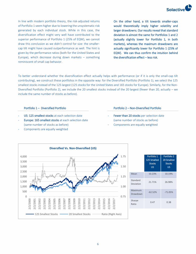
To better understand whether the diversification effect actually helps with performance (or if it is only the small-cap tilt
contributing), we construct these portfolios in the opposite way: for the Diversified Portfolio (Portfolio 1), we select the 125
smallest stocks instead of the 125 largest (125 stocks for the United States and 165 stocks for Europe). Similarly, for the Non-
Diversified Portfolio (Portfolio 2), we include the 20 smallest stocks instead of the 20 largest (fewer than 20, actually – we
include the same number of stocks as before).
Portfolio 1 – Diversified Portfolio
- US: 125 smallest stocks at each selection date
- Europe: 165 smallest stocks at each selection date
(same number of stocks as before)
- Components are equally weighted
Portfolio 2 – Non-Diversified Portfolio
- Fewer than 20 stocks per selection date
(same number of stocks as before)
- Components are equally weighted
Portfolio 1
125 Smallest
Stocks
US
Portfolio 2
20 Smallest
Stocks
US
Mean 10.23% 10.19%
Standard
Deviation 21.71% 26.98%
Maximum
Drawdown -62.52% -71.05%
Sharpe
Ratio 0.47 0.38
0.75
1.00
1.25
1.50
1.75
0
500
1,000
1,500
2,000
2,500
3,000
3,500
4,000
2/2
/20
00
2/2
/20
01
2/2
/20
02
2/2
/20
03
2/2
/20
04
2/2
/20
05
2/2
/20
06
2/2
/20
07
2/2
/20
08
2/2
/20
09
2/2
/20
10
2/2
/20
11
2/2
/20
12
2/2
/20
13
2/2
/20
14
2/2
/20
15
2/2
/20
16
2/2
/20
17
Diversified Vs. Non-Diversified (US)
125 Smallest Stocks 20 Smallest Stocks Ratio (Right Axis)
On the other hand, a tilt towards smaller-caps
would theoretically imply higher volatility and
larger drawdowns. Our results reveal that standard
deviation is almost the same for Portfolios 1 and 2
(actually slightly lower for Portfolio 1, in both
markets), whereas the maximum drawdowns are
actually significantly lower for Portfolio 1 (25% of
EQW). We can thus confirm the intuition behind
the diversification effect – less risk.
6

As we show in the next section, smaller caps outperform large caps in the US and Europe. In this light, it could be expected
that Portfolio 2 outperforms Portfolio 1, since the market capitalization of Portfolio 2 is smaller. However, it is Portfolio 1
(Diversified) that outperforms both in US and Europe. Volatility and maximum drawdowns are also significantly lower for the
Diversified Portfolios in both markets. The spikes in the ratios during the 2008 crisis confirm that the outperformance is due
to less risk and downside movement. Since the ratios do not decrease during bull markets (they stay constant in the United
States and increase in Europe), we can infer that the ratio spike in 2008 is not due to a larger cap tilt of Portfolio 1 (Diversified).
2. Higher Exposure to Small Cap Stocks
By construction, an EQW portfolio exhibits a substantially higher exposure to smaller cap stocks than a MCAP portfolio.
Historically, small caps generally show better performance. This characteristic is also intuitive: smaller companies have more
room to grow. This fact leads to the assumption that the higher exposure to small caps probably accounts for a substantial
part of the outperformance of equally weighted portfolios – an assumption that we will test in the final part of this paper,
when we break down the outperformance of EQW over MCAP portfolios.
Here however, we examine whether this size effect also occurs within relatively large caps – i.e. test if the smallest large-caps
outperform the largest large-caps. The reason for this analysis is the following: when comparing EQW and MCAP weighting
schemes using real-world Solactive indices, all the stocks in the composition will be relatively large. Thus, we again construct
two portfolios (actually four, since we are analyzing the size effect both for the United States and for Europe):
Portfolio 1 – Smallest 50 Stocks
- composed of the 50 smallest securities in the Solactive US Large Cap Index, and in the Solactive Europe Total Market 675 Index respectively.
- Components are equally weighted
Portfolio 2 – Largest 50 Stocks
- composed of the 50 largest securities in the Solactive US Large Cap Index, and in the Solactive Europe Total Market 675 Index respectively.
- Components are equally weighted
Portfolio 1
165 Smallest
Stocks
Europe
Portfolio 2
20 Smallest
Stocks
Europe
Mean 7.57% 5.22%
Standard
Deviation 17.78% 21.76%
Maximum
Drawdown -67.42% -78.12%
Sharpe
Ratio 0.43 0.24
0.50
0.75
1.00
1.25
1.50
1.75
2.00
0
500
1,000
1,500
2,000
2,500
3,0002
/2/2
00
0
2/2
/20
01
2/2
/20
02
2/2
/20
03
2/2
/20
04
2/2
/20
05
2/2
/20
06
2/2
/20
07
2/2
/20
08
2/2
/20
09
2/2
/20
10
2/2
/20
11
2/2
/20
12
2/2
/20
13
2/2
/20
14
2/2
/20
15
2/2
/20
16
2/2
/20
17
Diversified Vs. Non-Diversified (Europe)
165 Smallest Stocks 20 Smallest Stocks Ratio (Right Axis)
7

The ratios in both markets (United States and Europe) reveal that the 50 smallest
capitalization stocks perform worse during bear markets but also recover much faster
after downturns end, catching up and eventually overtaking the 50 largest capitalization
stocks. At the same time, these smaller cap stocks exhibit significantly larger drawdowns
than the large caps – still, they reach a higher level to fall from.
In the United States, the 50 smallest capitalization stocks act as expected: higher return
potential and volatility, though the trade-off indicated by the Sharpe ratio is still
advantageous. While in Europe they do offer better returns, the smaller capitalization
stocks are also surprisingly less volatile (and display a Sharpe ratio almost twice as good),
explaining why the EQW portfolio in Europe is less volatile than the MCAP weighted
portfolio.
Smallest 50
(US)
Largest 50
(US)
Mean 9.33% 6.54%
Standard
Deviation 23.63% 18.39%
Maximum
Drawdown -66.90% -50.93%
Sharpe
Ratio 0.39 0.36
Smallest 50
(Europe)
Largest 50
(Europe)
Mean 6.84% 3.92%
Standard
Deviation 19.61% 20.54%
Maximum
Drawdown -73.64% -60.02%
Sharpe
Ratio 0.35 0.19
0.90
1.00
1.10
1.20
1.30
1.40
1.50
500
1,000
1,500
2,000
2,500
3,000
3,500
2/2
/20
00
2/2
/20
01
2/2
/20
02
2/2
/20
03
2/2
/20
04
2/2
/20
05
2/2
/20
06
2/2
/20
07
2/2
/20
08
2/2
/20
09
2/2
/20
10
2/2
/20
11
2/2
/20
12
2/2
/20
13
2/2
/20
14
2/2
/20
15
2/2
/20
16
2/2
/20
17
Size Effect (US)
Smallest 50 Largest 50 Ratio (Right Axis)
0.60
0.80
1.00
1.20
1.40
1.60
1.80
250
500
750
1,000
1,250
1,500
1,750
2,000
2,250
2,500
2/2
/20
00
2/2
/20
01
2/2
/20
02
2/2
/20
03
2/2
/20
04
2/2
/20
05
2/2
/20
06
2/2
/20
07
2/2
/20
08
2/2
/20
09
2/2
/20
10
2/2
/20
11
2/2
/20
12
2/2
/20
13
2/2
/20
14
2/2
/20
15
2/2
/20
16
2/2
/20
17
Size Effect (Europe)
Smallest 50 Largest 50 Performance Ratio (Right Axis)
An important consideration:
due to the higher exposure to
smaller capitalization stocks, an
EQW index can have lower
investment capacity. This fact is
especially relevant for ETFs,
which might find an EQW index
more difficult to replicate. It is
also relevant for mutual funds
or institutional clients who need
to satisfy high capacities of
investments.
8

3. An Inherent “Buy Low & Sell High” Feature
Stock prices rise and fall over time. Assuming no component changes (i.e. no stocks in or out of the portfolio), a purely MCAP
weighted portfolio would not require weight adjustments from rebalancing to rebalancing, as the weights dictated by MCAP
are already reflected in the share prices – when a stock rises, its weight in an MCAP portfolio would also rise, and vice-versa.
Under the same assumption, maintaining equal weights among portfolio components still requires adjustments: selling some
shares of the stocks that appreciated in value, and buying more shares of the stocks whose prices fell. As a result, any gains
are effectively locked in, and are simultaneously used to increase exposure to the now cheaper underperformers. This
characteristic of an EQW portfolio is essentially a “buy low, sell high” trading strategy. If mean reversal in stock prices occurs,
an EQW portfolio is perfectly positioned to take advantage of this process and generate better returns over time.
In summary, we can say that an MCAP weighted portfolio is never adjusted (overlooking component additions or deletions),
whereas an EQW portfolio requires ongoing adjustments to maintain equal weight amongst its components. To test whether
this frequent portfolio rebalancing actually locks in gains and takes advantage of mean-reversal, we again build different
portfolios: one that is never rebalanced, and three that are increasingly frequently rebalanced (quarterly, weekly, and daily).
In order to isolate the effect of bringing stocks back to equal weight, we assume no component changes to the portfolio and
thus only include stocks that survived in the composition since the start of the simulation. We are aware of the resulting look-
ahead bias (explaining the very high index levels), but – again – we intend to isolate the rebalancing effect alone.
The composition of the following four portfolios is identical (169 stocks that survived in the Solactive US Large Cap Index since
2000), and all portfolios start equally weighted. The only difference is the rebalancing frequency.
The daily rebalanced portfolio
displays the highest returns,
followed by the weekly rebalanced,
quarterly rebalanced, and finally the
never rebalanced portfolios.
Of course, the turnover cost should
not be neglected, which would
reduce (if not entirely negate) any
excess returns generated by the
“rebalancing effect”. For more on
turnover, see the next section of this
paper.
In the graphs below, we focus on the
never rebalanced vs. the weekly
rebalanced portfolios, in order to
display the performance ratios,
which suggest that the frequently
rebalanced portfolio works best in
times immediately after crises or in
sideways markets.
Never Reb. (US) Qtrly. Reb. (US) Weekly Reb.(US) Daily Rebal. (US)
Mean 11.51% 12.17% 12.91% 13.30%
Standard Deviation 17.73% 18.70% 18.95% 19.00%
Maximum Drawdown -50.74% -52.26% -51.56% -50.39%
Sharpe Ratio 0.65 0.65 0.68 0.70
5001,0001,5002,0002,5003,0003,5004,0004,5005,0005,5006,0006,5007,0007,5008,000
2/2
/20
00
2/2
/20
01
2/2
/20
02
2/2
/20
03
2/2
/20
04
2/2
/20
05
2/2
/20
06
2/2
/20
07
2/2
/20
08
2/2
/20
09
2/2
/20
10
2/2
/20
11
2/2
/20
12
2/2
/20
13
2/2
/20
14
2/2
/20
15
2/2
/20
16
2/2
/20
17
Rebalancing Effect (US)
Never Rebalanced Quarterly Rebalanced
Weekly Rebalanced Daily Rebalanced
9

Portfolio 1 – Never Rebalanced
- composed of all the securities that remained in the Solactive US Large Cap Index (and in the Solactive Europe Total Market 675 Index) since 2000
- never adjusted
Portfolio 2 – Weekly Rebalanced
- composed of all the securities that survived in the Solactive US Large Cap Index (and in the Solactive Europe Total Market 675 Index) since 2000
- stocks brought back to equal weights weekly
According to these simulations, frequently bringing components back to equal weight has a noticeable, positive effect on
performance (though volatility and drawdowns increase). Furthermore, the more frequent the rebalancing, the better the
returns. Interestingly, our tests reveal that these results hold even when the portfolios start with MCAP weights, and are then
frequently brought back to these initial MCAP weights. However, an important aspect to consider are the turnover costs
(covered in the next section), which might render this “frequent rebalancing factor” impossible to capitalize on.
Never Reb.
(US)
Wkly Reb.
(US)
Mean 11.51% 12.91%
Standard
Deviation 17.73% 18.95%
Maximum
Drawdown -50.74% -51.56%
Sharpe
Ratio 0.65 0.68
Never Reb.
(Europe)
Wkly Reb.
(Europe)
Mean 9.64% 10.70%
Standard
Deviation 16.98% 19.00%
Maximum
Drawdown -57.34% -58.25%
Sharpe
Ratio 0.57 0.56
1.001.021.041.061.081.101.121.141.161.181.201.221.241.26
1,0001,5002,0002,5003,0003,5004,0004,5005,0005,5006,0006,5007,0007,500
2/2
/20
00
2/2
/20
01
2/2
/20
02
2/2
/20
03
2/2
/20
04
2/2
/20
05
2/2
/20
06
2/2
/20
07
2/2
/20
08
2/2
/20
09
2/2
/20
10
2/2
/20
11
2/2
/20
12
2/2
/20
13
2/2
/20
14
2/2
/20
15
2/2
/20
16
2/2
/20
17
Rebalancing Effect (US)
Never Rebalanced Weekly Rebalanced Ratio (Right Axis)
0.92
0.96
1.00
1.04
1.08
1.12
1.16
1.20
1.24
1.28
1.32
0
500
1,000
1,500
2,000
2,500
3,000
3,500
4,000
4,500
5,000
2/2
/20
00
2/2
/20
01
2/2
/20
02
2/2
/20
03
2/2
/20
04
2/2
/20
05
2/2
/20
06
2/2
/20
07
2/2
/20
08
2/2
/20
09
2/2
/20
10
2/2
/20
11
2/2
/20
12
2/2
/20
13
2/2
/20
14
2/2
/20
15
2/2
/20
16
2/2
/20
17
Rebalancing Effect (Europe)
Never Rebalanced Weekly Rebalanced Ratio (Right Axis)
10

11
4. Higher Portfolio Turnover
As aforementioned, the weights of market cap weighted portfolios adjust automatically with share price changes and require
redistribution of weights only under certain circumstances such as mergers or other extra-ordinary events. In the case of
equal weighting, the portfolio requires regular weight redistribution in order for the components to remain at equal weight.
Hence, an EQW portfolio will always imply higher turnover than a MCAP weighted one, regardless of the rebalancing
frequency – evident if we take a look at the average one-way turnover (per adjustment) of the following Solactive indices:
Solactive US Large Cap Index (MCAP)
3.62% mean one-way turnover (since 2000)
Solactive US Large Cap EQW Index
7.38% mean one-way turnover (since 2000)
Solactive Europe Total Market 675 Index (MCAP)
8.54% mean one-way turnover (since 2000)
Solactive Europe Total Market 675 EQW Index
18.11% mean one-way turnover (since 2000)
Thus, EQW portfolios imply higher
transaction costs, which can make
the difference between success and
failure. As an example, we can take
a look at the first attempts to launch
equal-weighted funds in the 70s. At
that point in time, the transaction
costs were considerably higher, and
the trading procedure more difficult,
leading to the establishment of the
MCAP weighting scheme as one of
the most common.
Today, however, transaction costs are
significantly lower, making the
equally weighted portfolios more
viable than in the past. Even if we
assume a very conservative
transaction cost of 50 basis points
(the transaction costs for non-retail
traders can be less than 10 bps), the
extra costs incurred by the quarterly
rebalanced EQW portfolios would still
be less than the excess returns
generated through weighting stocks
equally.
0%
2%
4%
6%
8%
10%
12%
14%
16%
18%
4/1
9/2
00
0
4/1
8/2
00
1
4/1
7/2
00
2
4/2
3/2
00
3
4/2
1/2
00
4
4/2
0/2
00
5
4/1
9/2
00
6
4/1
8/2
00
7
4/2
3/2
00
8
4/2
2/2
00
9
4/2
1/2
01
0
4/2
0/2
01
1
4/1
8/2
01
2
4/1
7/2
01
3
4/2
3/2
01
4
4/2
2/2
01
5
4/2
0/2
01
6
4/1
9/2
01
7
One Way Turnover (%) SOL US Large Cap Index
EQW MCAP
0%2%4%6%8%
10%12%14%16%18%20%22%24%
4/1
9/2
00
0
4/1
8/2
00
1
4/1
7/2
00
2
4/2
3/2
00
3
4/2
1/2
00
4
4/2
0/2
00
5
4/1
9/2
00
6
4/1
8/2
00
7
4/2
3/2
00
8
4/2
2/2
00
9
4/2
1/2
01
0
4/2
0/2
01
1
4/1
8/2
01
2
4/1
7/2
01
3
4/2
3/2
01
4
4/2
2/2
01
5
4/2
0/2
01
6
4/1
9/2
01
7
One Way Turnover (%) SOL Europe Total Market 675 Index
EQW MCAP

Outperformance Decomposition
Having established that EQW portfolios outperform MCAP weighted ones, and having analyzed their characteristics in detail,
we now decompose the outperformance in line with the points mentioned above, in order to better understand why and
how exactly they outperform:
1. Lower Concentration Risk (diversified vs. non-diversified portfolios)
2. Higher Exposure to Smaller-Cap Stocks (small vs large cap portfolios)
3. Inherent “Buy Low, Sell High” Feature (frequently vs unfrequently rebalanced portfolios)
In order to break down the outperformance, we need to construct different portfolios, treating each of these points as
factors. However, a problem immediately arises: the non-diversified portfolio is part of the diversified portfolio, and we
cannot build the other portfolios within these two. Furthermore, there is much overlap between our size and diversification
factors. Thus, we simply focus on the size factor and ignore the diversification one. The results are as follows:
In the case of both Solactive US Large Cap and Solactive Europe Total Market 675, most of the outperformance generated by weighting
equally is explained by the higher exposure to small cap stocks, whereas the rebalancing factor only has a minor effect.
In the United States, the small cap tilt explains about two thirds of EQW’s outperformance over MCAP, while in Europe it explains
slightly less than half. The rebalancing effect only explains about 5% of the performance difference in both markets.
To conclude, a stock’s size does not matter when weighting portfolios equally – all components receive the same proportions
regardless of size (in contrast to MCAP weighting). On the other hand, it seems that size is the most important factor when it comes
to the outperformance generated by the equally weighting.
Solactive US Large Cap Equal Weight
9.11%
Solactive US Large Cap (MCAP Weighted)
7.03%
Outperformance
2.08%
Non-Systematic 0.58%
Small Cap Tilt
1.38%
Rebalancing Effect 0.12%
Solactive Europe Total Market 675 Equal
Weight
7.21%
Solactive Europe Total Market 675(MCAP
Weighted)
5.07%
Outperformance
2.14%
Non-Systematic 1.07%
Small Cap Tilt
0.98%
Rebalancing Effect
0.09%
12

13
Appendix: Outperformance Decomposition
To decompose the excess returns of EQW over MCAP portfolios, we need to construct portfolios within portfolios treating
each of these points as factors:
1. Lower Concentration Risk (diversified vs. non-diversified portfolios)
2. Higher Exposure to Smaller-Cap Stocks (small vs large cap portfolios)
3. Inherent “Buy Low, Sell High” Feature (frequently vs unfrequently rebalanced portfolios)
Non-Diversified Diversified
Smaller Caps Larger Caps Smaller Caps Larger Caps
Weekly Reb. (Portf. 1)
Annual Reb. (Portf. 2)
Weekly Reb. (Portf. 3)
Annual Reb. (Portf. 4)
Weekly Reb. (Portf. 5)
Annual Reb. (Portf. 6)
Weekly Reb. (Portf. 7)
Annual Reb. (Portf. 8)
As previously mentioned, we focus on the size factor and ignore the diversification one, since we cannot build the other
portfolios within the Diversified/Non-Diversified ones and since there is considerable overlap anyway between the size and
diversification factor as we have defined it earlier.
Hence, we build four portfolios: 50% smallest stocks
rebalanced annually, 50% smallest stocks rebalanced
weekly, 50% largest stocks rebalanced annually, and 50%
largest stocks rebalanced weekly (see left). All portfolio
members are equally weighted.
We have back-tested each of these four portfolios and obtained daily returns for each. We construct the well-known SMB
factor (Small minus Big) and our “Rebalancing Factor” in the following way:
Small Minus Big (daily returns) =
[(SmallWeekly + SmallAnnually) – (LargeWeekly + LargeAnnually)] ÷2
Weekly Minus Annual (daily returns) =
[(SmallWeekly + LargeWeekly) – (SmallAnnually + LargeAnnually)] ÷2
Over our back-test period (Feb 2000 to Oct 2017), going long on the 50% smallest companies in the Solactive US Large Cap
Index while shorting the 50% largest yielded an annual mean return of 2.56%. In the case of Solactive Europe Total Market
675 Index, the size factor displayed a return of 1.33% per year. Going long on the weekly rebalanced portfolios and shorting
the annually rebalanced portfolios yielded 0.70% per year in the United States and 0.51% in Europe.
Regressing the returns of these two factors on the excess returns of EQW over MCAP, the size factor displays a beta of 0.54
in the US and 0.74 in Europe. The rebalancing factor exhibits a beta of 0.18 in the United States, and 0.17 in Europe (both
factors are statistically significant @ 95%).
Smaller Caps Larger Caps
Weekly Reb. (Portf. 1)
Annual Reb. (Portf. 2)
Weekly Reb. (Portf. 3)
Annual Reb. (Portf. 4)

14
In order to better visualize how these factors performed since the year 2000, we plot the effect of these excess returns on a
starting level of 1,000 (see below). Furthermore, we also plot the performance of going long on EQW and shorting MCAP
(EQW-MCAP, also starting at 1,000). Please note that the rebalancing factor is plotted on the right axis, due to its lesser
magnitude.
These graphs summarize and strengthen
our previous findings:
- EQW-MCAP drops during market
downturns, but grows during bull markets.
- Small-Big displays similar behavior.
- Interestingly, Weekly-Annual acts the
same way, dropping during the financial
crisis. The explanation is that the
rebalancing effect is a double-edged
sword: it will keep increasing exposure to
dropping stocks. If mean reversal occurs,
the ‘rebalancing effect’ would work in our
favor, but if these stocks keep dropping to
the point of bankruptcy, the “rebalancing
effect” would actually increase losses.
950
975
1,000
1,025
1,050
1,075
1,100
1,125
1,150
1,175
800
900
1,000
1,100
1,200
1,300
1,400
1,500
1,600
1,700
2/2/2000 2/2/2004 2/2/2008 2/2/2012 2/2/2016
Plotted Factors (US)
EQW-MCAP Small-Big Weekly-Annual (Right Axis)
950
975
1000
1025
1050
1075
1100
1125
800
900
1000
1100
1200
1300
1400
1500
2/2/2000 2/2/2004 2/2/2008 2/2/2012 2/2/2016
Plotted Factors (Europe)
EQW-MCAP Small-Big Weekly-Annual (Right Axis)

Contact
SOLACTIVE AG
German Index Engineering
Guiollettstr. 54
60325 Frankfurt am Main
www.solactive.com
Timo Pfeiffer, Head of Research & Business Development
+49 (69) 719 160 320
Emanuel Cozmanciuc, Quantitative Research Analyst
+49 (69) 719 160 313
Fabian Colin, Head of Sales
+49 (69) 719 160 220
Follow us on
Disclaimer
Solactive AG does not offer any explicit or implicit guarantee or assurance either with regard to the results of using an Index and/or
the concepts presented in this paper or in any other respect. There is no obligation for Solactive AG - irrespective of possible
obligations to issuers - to advise third parties, including investors and/or financial intermediaries, of any errors in an Index. This
publication by Solactive AG is no recommendation for capital investment and does not contain any assurance or opinion of Solactive
AG regarding a possible investment in a financial instrument based on any Index or the Index concept contained herein. The
information in this document does not constitute tax, legal or investment advice and is not intended as a recommendation for
buying or selling securities. The information and opinions contained in this document have been obtained from public sources
believed to be reliable, but no representation or warranty, express or implied, is made that such information is accurate or complete
and it should not be relied upon as such. Solactive AG and all other companies mentioned in this document will not be responsible
for the consequences of reliance upon any opinion or statement contained herein or for any omission.
All numbers are calculated by Solactive as of Q4 2017.


