Journal of AI and Data Mining
Vol 5, No 1, 2017, 89-100 DOI: 10.22044/jadm.2016.655
Using a new modified harmony search algorithm to solve multi-objective
reactive power dispatch in deterministic and stochastic models
Kh. Valipour* and A. Ghasemi
Technical Engineering Department, University of Mohaghegh Ardabili, Ardabil, Iran.
Received 12 January 2016; Accepted 30 May 2016 *Corresponding author: [email protected] (Kh. Valipour.)
Abstract
The optimal reactive power dispatch (ORPD) problem is a very important aspect in power system planning,
and it is a highly non-linear, non-convex optimization problem because it consists of both the continuous and
discrete control variables. Since a power system has an inherent uncertainty, this paper presents both the
deterministic and stochastic models for the ORPD problem in multi-objective and single-objective
formulations, respectively. The deterministic model considers three main issues in the ORPD problem
including the real power loss, voltage deviation, and voltage stability index. However, in the stochastic
model, the uncertainties in the demand and equivalent availability of shunt reactive power compensators
have been investigated. To solve them, we proposed a new modified harmony search algorithm (HSA),
implemented in single and multi-objective forms. Since, like many other general purpose optimization
methods, the original HSA often traps into the local optima, an efficient local search method called chaotic
local search (CLS) and a global search operator are proposed in the internal architecture of the original HSA
algorithm to improve its ability in finding the best solution because the ORPD problem is very complex, with
different types of continuous and discrete constrains, i.e. excitation settings of generators, sizes of fixed
capacitors, tap positions of tap changing transformers, and amount of reactive compensation devices.
Moreover, the fuzzy decision-making method is employed to select the best solution from the set of Pareto
solutions. The proposed model is individually examined and applied on different test systems. The
simulation results show that the proposed algorithm is suitable and effective for the reactive power dispatch
problem compared to the other available algorithms.
Keywords: Reactive Power Dispatch, Modified HSA, Multi-objective, System Stability, Stochastic Model.
1. Introduction
The optimal reactive power dispatch (ORPD)
problem can be divided into two parts, known as
the real and reactive power dispatch problems.
The real power dispatch problem aims to
minimize the total cost of real power generation
from thermal power plants at various stations [1].
However, reactive power dispatch controls the
power system stability and power quality, i.e.
voltage stability and power loss. Generally, the
objective of ORPD is to minimize the real power
loss and increase the voltage stability in the power
system, while satisfying various discrete and
continues constraints [2].
Recently, many scientific papers have been
dedicated to the ORPD problem, which can be
classified into two groups, classical and intelligent
computing methods. Classical computing methods
consist of some well-known mathematical
strategies such as linear programming (LP) [3],
non-linear programming (NLP) [4], quadratic
programming [5], and decomposition technique
[6]. This group is computationally fast but they
have several limitations like (i) the need for
continuous and differentiable objective functions,
(ii) easy convergence to local minima. and (iii)
difficulty in handling a very large number of
variables. Therefore, it is vital to develop some
intelligent methods that are capable of
overcoming these shortages. In another group,
computational intelligence-based techniques have
been proposed for the application of reactive
power optimization. In [7], a new modified
Valipour & Ghasemi/ Journal of AI and Data Mining, Vol 5, No 1, 2017.
90
version of honey bee mating optimization called
the parallel vector evaluated honey bee mating
optimization (PVEHBMO) based on multi-
objective formulation has been proposed to solve
the RPD problem. In [8], the authors have
presented a quasi-oppositional differential
evolution to solve the ORPD problem of a power
system. In [9], the authors have proposed a multi-
objective differential evolution (MODE) to solve
the multi-objective optimal reactive power
dispatch (MORPD) problem by minimizing the
active power transmission loss and voltage
deviation, and maximizing the voltage stability,
while varying the control variables such as the
generator terminal voltages, transformer taps, and
reactive power output of shunt compensators.
Pareto-efficient 12-h variable double auction
bilateral power transactions have been considered
in [10]. The effect of that on the economic welfare
has been observed, while solving the reactive
power dispatch (RPD) by differential evolution
using the random localization technique. This has
been accomplished by a combination of static and
dynamic var compensators. Out of these 12-h
variable power transactions, the Pareto-efficient
transactions, which are reconciled by planed
biding, have provided the maximum global
welfare. In [11], the authors have presented a new
meta-heuristic method, namely gray wolf
optimizer (GWO), which is inspired from gray
wolves’leadership and hunting behaviors to solve
the optimal reactive power dispatch (ORPD)
problem.
The aforementioned papers show that the
optimization methods have a good potential to
solve the ORPD problem. The ORPD with high
optimal variables and constrains requires a more
effective method to avoid the local optimal
solutions, and it has well-distribution of non-
dominated solutions, while satisfying the diversity
characteristics. A new meta-heuristic algorithm,
mimicking the improvisation process of music
players, has been recently developed and named
the harmony search algorithm (HSA) [12]. Due to
its many positive features, being simple in concept
and easy to implement, flexibility, the possibility
of using chaotic maps and of developing hybrids
from combinations with other techniques, the
HSA algorithm has been successfully applied to
the optimization of complex mathematical
functions with or without constraints [13].
Unfortunately, the standard HSA often converges
to local optima. In order to improve the fine-
tuning characteristic of HSA, an improved HSA
has been proposed, enhancing the fine-tuning
characteristic and convergence rate of harmony
search [14-15]. This paper proposes two
modifications in the local and global operators. In
the local term, a new CLS operator is presented to
update each particle in the search space. In the
global part, the pitch adjusting rate (PAR) and the
distance bandwidth (bw) are rewritten, which are
important coefficients in exploration and
exploitation. Moreover, HSA is developed as a
stochastic optimization algorithm; it can find an
optimal solution within a short calculation time.
The results obtained from three test systems in the
ORPD problem show that the proposed method
has a robust convergence and makes an acceptable
distribution in the Pareto-optimal solutions.
2. Deterministic formulation of ORPD problem
In this section, the deterministic formulation of
the ORPD problem is presented.
2.1. Problem objectives
• Objective 1: power-loss minimization
Transmission losses are construed as a loss of
revenue by the utility. The transmission loss can
be expressed by [7]:
2 2
1
1
P ( , ) [ 2 cos( )LN
loss k i j i j i j
k
J x u g V V V V
(1)
where, gk is the conductance of the line i-j, Vi and
Vj are the line voltages, and θi and θj are the line
angles at the i and j line ends, respectively, k is the
kth network branch that connects bus i to bus j, i =
1, 2, . . , ND, where ND is the set of numbers of
power demand bus, and j = 1, 2, . . . , Nj, where Nj
is the set of numbers of buses adjacent to bus j.
PG is the active power in lines i and j. x and u are
the vector of dependent variables and the vector of
control variables, respectively.
• Objective 2: Minimization of voltage deviation
The aim of this function is to minimize the
absolute voltage deviation of load bus voltages
from their desired values:
2
1
( , ) | |Nd
spi i
i
J VD x u V V
(2)
where, Nd is the number of load buses.
• Objective 3: Minimization of L-index voltage
stability
It is a static voltage stability measure of power
system, which is computed based on the normal
load flow solution. L-index Lj of the jth bus can be
expressed by:
1
11 2
1 , 1,2,...,
[ ] [ ]
PVNi
j ji PQji
ji
VL F j N
V
F Y Y
(3)
where, NPV and NPQ are the number of PV and PQ

Valipour & Ghasemi/ Journal of AI and Data Mining, Vol 5, No 1, 2017.
91
buses, respectively. Y1 and Y2 refer to the sub-
matrices of the YBUS matrix one gets:
1 2
3 4
PQ PQ
PV PV
I VY Y
Y YI V
(4)
The L-index is calculated for all the PQ buses. Lj
shows no load case and voltage collapse
conditions of bus j in the range of (0, 1). Thus the
objective function is represented by:
max( ), 1,2,...,j PQL L j N (5)
In the ORPD problem, an incorrect set of control
variables may increase the value of L-index, and
leads to a voltage instability. Let the maximum
value of L-index be Lmax. Therefore, to enhance
the voltage stability, and to keep the system far
from the voltage collapse margin, one gets:
3 max( , )J VL x u L (6)
2.2. Objective constraints
• Constraints 1: Equality Constraints
In the ORPD problem, the power generation must
be equal to the sum of the demand (PD) and the
power loss in the transmission lines:
1
1
[ cos( ) sin( )]
[ sin( ) cos( )]
B
i i
B
i i
N
G D i j ij i j ij i j
j
N
G D i j ij i j ij i j
j
P P V V G B
Q Q V V G B
(7)
where, NB is the number of buses; QGi is the
reactive power generated at the ith bus; and PDi
and QDi are the ith bus load real and reactive
power, respectively; Gij and Bij are the transfer
conductance and susceptance between bus i and
bus j, respectively; Vi and Vj are the voltage
magnitudes at bus i and bus j, respectively; and θi
and θj are the voltage angles at bus i and bus j,
respectively.
• Constraints 2: Generation Capacity Constraints
Generally, the generator outputs and bus voltage
constrains by lower and upper limits are as follow: min max min max,i i i i i iQ Q Q v v v (8)
Where, Pimin
and Pimax
are the minimum and
maximum values, respectively.
• Constraints 3: Line-flow constraints
One of the main constrains in the ORPD problem
is the maximum transfer capacity of the
transmission line. These constrains can be
calculated as follows: max
, , , 1,2,...,Lf k Lf kS S k L (9)
where, SLf,k is the real power flow of line k; max
,Lf kS
is the power flow upper limit of line k, and
subscript L denotes the number of transmission
lines.
• Constraints 4: Transformer
The transformer tap setting is restricted by its
lower and upper values: min max
i i iT T T (10)
2.3. Problem formulation
As results, the proposed deterministic multi-
objective ORPD problem can be formulated as:
2 31
,
T T T TL G L
T T T TG C
min[P ( , ) , ( , ) , ( , )]
:
( , ) 0
( , ) 0
, x = [[V ] , [Q ] , [S ] ],
u = [[V ] , [T] , [Q ] ]
lossx u
J JJ
x u VD x u VL x u
subject to
g x u
h x u
where
(11)
Where, g and h are the equality and inequality
constraints, respectively; [VL], [QG], and [SL] are
the vector of load bus voltages, generator reactive
power outputs, and transmission line loadings,
respectively; and [VG], [T], and [QC] are the vector
of generator bus voltages, transformer taps, and
reactive compensation devices, respectively.
3. Stochastic formulation of ORPD problem
In practice, power injections, especially from
intermittent renewable sources, and demand are of
uncertainties [16-17]. To aim with this cope, in
this section, the load uncertainty is developed in
the stochastic form in the ORPD problem. Usually
the probability distribution of a random variable is
represented using a finite set of scenarios. In other
words, each scenario (sth) has an associated
probability of occurrence (ξs). From (1), variable
can be defined as:
n
n L
pL
(12)
The expected value for can be given by:
,[ ] . . . (13)s s s n s n s
s S s S n TL s S n TL
E pL pL
Substituting (12) and (13), one gets:
min{ ( ) [ ( )]}f x E y (14)
Finally, the stochastic formulation of power loss
can be calculated as follows:
,, , ,
,
, , , ,
, , , ,
, , ,
, ,
min .
( , , )
( , , )
, ,
, | |
{ , , ,
SH
slack G
s n sv tab q
s S n TLP q
G G D
p s slack s l s i s
G D SH
j s l s i s k s
G G G SH SH SH
j j s j k k s k i i s i
m s n s nmm
f pL
P p P P v tab
q Q Q v tab q
Q q Q Q q Q V v V
Tap tap Tap s S
i B k SH p PV j
{ },
, , , }
PV slack
l PQ m TAP n TL s S
(15)

Valipour & Ghasemi/ Journal of AI and Data Mining, Vol 5, No 1, 2017.
92
Constraints Eqs. (7)-(11) in the deterministic
model are modified to take into account all the
different scenarios of demand s S , such that
modifications are shown in constraints Eq. (15) in
the stochastic model.
4. Multi-objective MHSA
4.1. Standard HSA
In this section, the original HSA is briefly
introduced; more details can be found in [12].
Start
Objective function f(x), x=(x1,x2, …,xd)T
Generate initial harmonics (real number arrays) Define pitch adjusting rate (PAR), pitch limits and bandwidth
Define harmony memory accepting rate (raccept)
while t<Max number of iterations Generate new harmonics by accepting best harmonics
Adjust pitch to get new solutions
if (rand>raccept), choose an existing harmonic randomly else if (rand>PAR), adjust the pitch randomly within limits
else generate new harmonics via randomization
end if
Accept the new harmonics (solutions) if better
end Find the current best solutions
End
Figure 1. Pseudo-code of standard HSA.
This algorithm has three main components, as
shown in figure 1. It is clear that the probability of
randomization can be given by:
random acceptP =1-r (16)
and the actual probability of adjusting pitches is
given by:
pitch acceptP =r PAR (17)
4.2. Modified HSA
This algorithm shows a good performance in an
optimization problem, although the main shortage
of the HSA algorithm comes from this fact that it
may miss the optimum solution or converge to a
near optimum solution. However, it has a flexible
and well-balanced mechanism to enhance the
global and local exploration abilities. Therefore,
the following modifications are proposed.
Modification of bw and PAR
Generally, the parameters PAR and bw are
arbitrarily fixed. It is clear that they can affect the
stochastic nature of HSA. Therefore, a time-
varying operator is proposed to keep away from
this difficulty:
min max min( )i
iPAR PAR PAR PAR
H (18)
min
maxmax
ln( )
exp( )i
bw
bwbw bw i
H (19)
where, PARmin and PARmax are the minimum and
maximum values for the pitch adjustment rate in
the search space, respectively; and H and i are the
maximum and current iterations, respectively.
• Global searching operator
In order to have an effective global search,
combine the genetic operator as follows:
min max min
i=1:N
( );
;
rand T
rand ( );
best worsti i i
New besti i i
Newi i i i
for
penalty abs x x
x x penalty
if
x x x x
end
end
(20)
The superscripts best and worst refer to the global
best and worst solutions for variable x,
respectively. The parameter penalty is the
guarantee for the global search ability. In other
words, after some evaluations, HSA may reach a
local solution and penalty goes to zero, and
hereby, the algorithm will be stagnated. To avoid
this shortage, generate some random harmonies,
and replace the worse harmonies. The number of
new random harmonies depends on the problem
and size of HM. The new random harmonies
increase the penalty parameter, and lead to new
exploration in finding a better solution.
• Local searching operator (CLS)
Chaos is a random-like process found in a non-
linear, dynamical system, which is non-period,
non-converging, and bounded [17]. The proposed
CLS-integrated HSA can be formulated as
follows:
1
2 , 0 0.5, 1,2,...,
2(1 ), 0.5 1
j j
i ij
i j j
i i
c if cc j Ng
c if c
(21)
where, Cji+1 is the j
th chaotic variable of i
th
iteration. This combination can be summarized as
follows:
i) Generate an initial population: 0 1 2
,0 ,0 1,0
1 20 0 0 0
,min,0
0,max ,min
[ , ,..., ]
[ , ,..., ]
, 1,2,...,
g
Ngcls cls cls Ncls
Ng
jjclsj
j j
X X X X
cx cx cx cx
X Pcx j Ng
P P
(22)
where, the chaos variable can be obtained by: 1 2
, , 1,
,max ,min ,min, 1
[ , ,..., ] , 1,2,...,
( ) , 1,2,...,
g
Ngicls cls i cls i N chaoscls i
j jj j j gcls i i
x x x x i N
x cx P P P j N
(23)
ii) Measure the chaotic variables:
Valipour & Ghasemi/ Journal of AI and Data Mining, Vol 5, No 1, 2017.
93
1 2
1
0
[ , ,..., ], 0,1,2,...,
1,2,...,
(0)
Ngi i i choasi
ji
j
cx cx cx cx i N
cx base CLS j Ng
cx rand
(24)
where, Nchaos is the number of individuals for
CLS; Ngicx is the i
th chaotic variable; rand() is a
random number at the range (0,1); Ng is the
number of units; and Xicls is the current position of
the harmony-based chaos theory.
iii): Map the decision variables
iv): Convert the chaotic variables to the decision
variables
v): Evaluate the new solution with decision
variables.
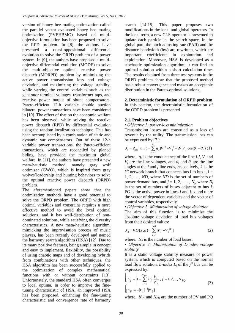
4.3. Non-dominated sort and crowding distance
In this process, the entire population is sorted with
its non-dominated level. Each solution is assigned
with a fitness value. Perform the non-dominated
sort method on the initial population, and
calculate the rank: rank1, rank2, rank3...., etc.
After the non-dominated sort is done, the
crowding distance is assigned to each solution.
The crowding distance is assigned front wise.
Compare the crowding distance between two
individuals in different fronts [9, 10]. Hereby, the
density of the surrounding individuals of i is
expressed by id, which is the smallest range that
contains i but does not contain other points around
the individual i . This process can be expressed as
follows:
i) For each front iF , l is the number of
individual, i.e. | |iF l .
ii) For every individual i , set the initial crowding
distance 0di .
iii) Set 1d dl . For each individual i , [ ].P i k
denotes the value for the thk objective function.
iv) Let i cycle be from 2 to 1l , and calculate the
following expression to define the crowding
distance for each individual
(25)
The graphical outlook for non-dominated sort and
crowding distance is shown in figure 2.
4.4. Best compromise solution
Fuzzy decision-maker is one of the multi-criteria
decision methods that provide the best decision
between a set of solutions. It can help the designer
to make the best decisions that are consistent with
their values, goals, and performances [17].
Hereby, firstly, the solution is assigned with the
following triangular membership function:
max
max min
i i
i
i i
f f
f f
(26)
0 0
0 1
1 1
i
i i i
i
FDM
(27)
where, fimin and f
imax are the maximum and
minimum values for the ith function response of
the selected kth solution, respectively. The
normalized membership function FDMk can be
calculated by: obj
obj
N
1
N
1 1
k
ik i
Mj
i
j i
FDM
FDM
FDM
(28)
where, M is the number of non-dominated
solutions, and Nobj is the number of objective
functions. Figure 3 illustrates a typical shape of
the employed membership function.
Figure 2. Non-dominated and crowding distance sorting.
Figure 3. Membership function.
4.5. Pareto-optimal solutions
For a problem with J objectives (o1, o
2, …, o
J), a
solution s = (os1, os
2, …, os
J) dominates another
one s′ = (os′1, os′
2, …, os′
J) if both of the following
conditions are satisfied [21]:
s is no worse than s′ in any attributes
m
k kk
kkdd
ff
fiPfiPii
1
minmax
)].1[].1[(
max
ifmin
if
1
0
i
if
Valipour & Ghasemi/ Journal of AI and Data Mining, Vol 5, No 1, 2017.
94
s is strictly better than s′ in at least one
attribute.
It can be denoted as s ≻ s′ or s′ ≺ s. A solution s is
defined as covering another one s′ if s is no worse
than s′ in any attribute. It can be denoted as s ≽ s′
or s′ ≼ s.
If a solution s cannot be dominated by another one
s′, it can be said that s is non-dominated by s′. If a
solution s is non-dominated by all the other
solutions in a solution set , it is called the
Pareto-optimal solution in . The set of all the
non-dominated solutions of is called the Pareto-
set of .
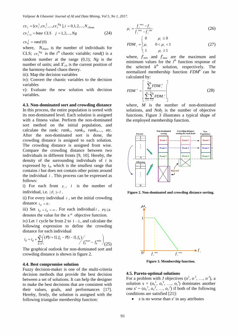
5. Applying MHSA in a multi-objective ORPD
problem
The proposed strategy to solve ORPD in the
multi-objective framework can be stepped as
follows:
Step 1: Generate the initial populations. Firstly,
set counter i = 0, and generate n random harmony,
as follows: 1 2
1 2 3[ , , ,..., ] ( , ,..., )m
n i i i iD D D D D D d d d (29)
where dij is the j
th state variable value of the i
th
harmony population. For each individual (Di), the
objective function values are calculated.
Step 2: The three conflicted fitness functions,
namely J1, J2, and J3 should be minimized
simultaneously, while satisfying the system
constraints.
Step 3: Update the counter i= i +1.
Step 4: Store the positions of the solutions that
represent the non-dominated vectors.
Step 5: Determine the best global solution for the
ith harmony from the non-dominated sort. First,
these hypercubes consisting of more than one
solution are assigned a fitness value equal to the
result of dividing any number x>1 by the number
of solutions that they contain. Then apply the
crowding distance on the fitness values to select
the hypercube.
Step 6: Generate a new population of harmonies
based on the proposed mutation, local and global
operators.
Step 7: Evaluate each solution by the Newton-
Raphson power flow analysis method to calculate
the power flow and system transmission loss.
Step 8: Update the contents of the repository non-
dominated sort together with the geographical
representation of the solutions within the
hypercube.
Step 9: Update the contents of the repository
solutions.
Step 10: If the maximum iteration itermax is
satisfied, then the stop optimization process and
print final results. Otherwise, go to step 3.
The graphical illustration is shown in figure 4.
Figure 4. Proposed strategy to solve ORPD problem with modified HAS method.
Yes
No Yes
No
Use CLS mechanism to enhance local search and modified current
solution
START
Set algorithm parameters and generate initial population and chaos solutions
Calculate objective functions values
Dominated solutions Pareto front
Non-dominated solution
f1
f2
f1(x)
f2(x)
Fuzzy mechanism for best comparison
max
ifmin
if
1
0i
f
i
Generate new solutions by proposed global search or crossover
Is termination
criteria satisfied?
End
All solution are
distributed?
Calculate objective function values
Calculate objective function values
Compare best solution and memorize best one
Generate new
solution and
replace with worth of pervious
sections
1
1

Valipour & Ghasemi/ Journal of AI and Data Mining, Vol 5, No 1, 2017.
95
6. Simulation and discussion
The proposed algorithm was implemented in the
MATLAB language 2011a. All simulations were
performed on a PC with an Intel Duo Core
processor T5800, 2 GHz with a 4GB RAM. In
order to access full search ability of the proposed
algorithm, test it on the several benchmarks and
look at the other articles. As a result, PARmin,
PARmax, bwmin, and bwmax were set with the 0.35,
0.99, 5×10⁻⁴, and 0.05 values, respectively.
HMCR and HMS were 0.95 and 4, respectively.
Also the maximum number of iterations was equal
to 500.
6.1. Deterministic model on IEEE 14-bus
At first, the IEEE 14-bus test system was
considered with five generator buses (bus 1 was
the slack bus, and buses 2, 3, 6, and 8 were PV
buses with continuous operating values), 9 load
buses and 20 branches, in which 3 branches (4-7,
4-9, and 5-6) were tap changing transformers.
Moreover, the candidate buses for shunt
compensation were 9 and 14.
Table 1. Results of multi-objective optimization in IEEE
14-bus test system.
Parameters Case 1 Case 2
MHSA HSA MHSA HSA
Vg2 1.012 1.034 1.132 1.098
Vg3 1.031 1.065 1.074 1.109
Vg6 1.029 1.095 1.030 1.165
Vg8 1.065 1.082 1.072 1.163
T4-7 1.012 1.034 1.028 1.064
T4-9 0.970 0.976 0.907 1.006
T5-6 0.952 0.897 0.989 0.943
Qc9 0.324 0.302 0.302 0.325
Qc14 0.058 0.047 0.073 0.049
J1 1.176 1.209 1.175 1.206
J2 0.205 0.243 0.298 0.652
J3 0.137 0.135 0.113 0.120
Parameters Case 3 Case 4
MHSA HSA MHSA HSA
Vg2 1.093 1.103 1.083 1.053
Vg3 1.065 1.095 1.094 1.064
Vg6 1.083 1.163 1.028 1.093
Vg8 1.001 1.154 1.014 1.172
T4-7 1.039 1.196 1.004 1.106
T4-9 1.042 0.895 1.042 0.953
T5-6 0.987 0.854 0.987 0.803
Qc9 0.393 0.473 0.386 0.401
Qc14 0.063 0.035 0.057 0.038
J1 1.195 1.268 1.177 1.210
J2 0.203 0.438 0.208 0.448
J3 0.114 0.123 0.115 0.125
In order to evaluate the effectiveness of the
proposed algorithm in this test system, four
different cases were considered as follow:
Case 1: Consider two objective functions; real
power loss (J1) and voltage deviation (J2).
Case 2: Consider two objective functions; real
power loss (J1) and voltage stability index (J3).
Case 3: Consider two objective functions; voltage
deviation (J2) and voltage stability index (J3).
Case 4: Consider all objective functions; J1, J2,
and J3.
The numerical results of these case studies with 9
variables were tabulated in table 1, satisfying the
system constrains. In all cases, the lower and
upper limits of reactive powers were 0-30 MVAr,
and these limits for the transformer tap settings
and voltage magnitude were considered within the
interval 0.9-1.1 p.u, respectively. The simulation
results for the algorithms are shown in table 2. It
can be seen that the results obtained for MHSA
are better than those for the standard HSA
algorithm in all cases. The Pareto front of the
proposed algorithm for all cases is shown in figure
5.
Moreover, in order to show the robustness of the
proposed algorithm to solve the ORPD problem,
consider all objective functions, and optimize
them by 30 trails that were individually run for 30
times. The simulation results of these trails are
given in figure 6.
Figure 6. Distribution of final results for proposed
algorithm in 30 trials, which simultaneously optimize
three objective functions.
It is clear that the variation range of the best total
cost during 30 trails simulations is small, which
indicates that the MHSA algorithm is stable
compared to HSA.
6.2. Deterministic model on IEEE 30-bus
The proposed algorithm was carried out on the
IEEE 30-bus test system, which consisted of six
thermal plants, 26 buses, and 46 transmission
lines. The other useful line data and bus data were
taken from [7]. Moreover, it had four
transformers, with the off-nominal tap ratio at
lines 6–9, 6–10, 4–12, and 28–27. In addition,
buses 10, 12, 15, 17, 20, 21, 23, 24, and 29 were
selected as shunt VAR compensation buses.
The results of the proposed algorithm were
compared with SGA, PSO, GSA, standard HAS,
etc, all of which were referred to [7] and [18]. The
load of system was Pload = 2.832 p.u and Qload =
0 5 10 15 20 25 301.174
1.176
1.178
1.18
Trail number
Plo
ss (
MW
)
MHSA
HSA
0 5 10 15 20 25 300.2
0.3
0.4
0.5
0.6
Trail number
Vo
ltag
e d
ev
iati
on
MHSA
HSA
0 5 10 15 20 25 300.1
0.12
0.14
0.16
Trail number
Vo
ltag
e s
tab
ilit
y (
L-i
nd
ex
)
MHSA
HSA

Valipour & Ghasemi/ Journal of AI and Data Mining, Vol 5, No 1, 2017.
96
1.262 p.u on a 100 MVA base. In this case, the
optimization problem had 19 control variables,
which were presented in table 2.
Figure 5. Pareto-optimal front of proposed approach, IEEE 14 bus.
Table 2. Variable limits (p.u.). Voltage and tab setting limits Reactive power generation limits
11 8 5 2 1 Bus 13 11 8 5 2 1 Bus
Tmin Tmax Vloadmin Vload
max VGmin VG
max 0.155 0.15 0.53 0.6 0.48 0.596 QGmax
0.95 1.05 0.95 1.05 0.9 1.1 -0.078 -0.075 -0.265 -0.3 -0.24 -0.298 QGmin
Reactive compensation devices and voltage limits
VGmax VG
min VGmax QC
max
0.95 1.05 -0.12 0.36
Table 3. Comparison of transmission loss for different methods in IEEE 30-bus system. Algorithm GAMs PSO [7] HSA [7] DE [7] SQP [7] GSA [7] BBO [7] BF [18]
Best Ploss (MW) 4.5468 4.9239 4.9059 5.011 5.043 4.51431 4.5511 4.623
Worst Ploss (MW) 4.8932 5.0576 4.9653 --- --- --- --- 4.64
Average Ploss (MW) 5.1029 4.9720 4.9240 --- --- --- --- 4.68
CPU time, s 11.82 --- --- --- --- 94.6938 --- ---
Algorithm CPVEIHBMO [7] BF [18] ABC [18] FF [18] HBMO [7] HFA [18] ALC-PSO [18] MHSA
Best Ploss (MW) 4.37831 4.623 4.6022 4.5691 4.40867 4.529 4.4793 4.373
Worst Ploss (MW) 4.4901 4.64 4.61 4.578 4.8869 4.5325 4.5036 4.487
Average Ploss (MW) 4.4826 4.68 4.63 4.59 4.6453 4.546 4.4874 4.480
CPU time, s 66.038 --- --- --- 67.413 --- --- 65.02
The simulation results were tabulated in table 3.
As it is evident in this table, the proposed method
demonstrates its superiority in the ORPD
problem, success rate, and solution quality over
the other heuristic methods. Moreover, these
results confirm the potential of multi-objective
MHSA algorithm to solve real-world highly non-
linear constrained multi-objective optimization
problems. For the sake of a fair comparison, the
results obtained by the MHSA algorithm in term
of power loss reduction were compared with the
other algorithms [7], in which the constraints and
initial settings of the problem were different with
the assumed values and constraints (four reactive
compensation devices were installed at buses 6,
17, 18, and 27). Figure 7 shows a comparison
between the different algorithms. The results
obtained show that the proposed method
demonstrates its superiority in computational
complexity, success rate, and solution quality over
the PSO, GSA, HSA, HBMO, IPM, and DE
methods. For the sake of a fair comparison among
the developed methods, 10 independent runs were
carried out.
6.3. Deterministic model on IEEE 118-bus
For the completeness and comparison purposes,
this is the largest practical test system which we
0
P0.2 0.22 0.26 0.28 0.301 0.302
1.175
1.181
1.184
Voltage deviation
Plo
ss (
MW
)
1.186
Case 1
HSA
MHSA
0.200 0.215
0.226 0.264
0.142 0.132
0.121 0.111
0.10
1.20
1.20
1.2
1.31
Voltage deviation
Voltage stability (L-index)
0 0.113 0.114 0.115 0.12 0.121 0.122
1.175
1.181
1.184
Voltage stability (L-index)
Plo
ss (
MW
)
1.186
Case 2
HSA
MHSA
0 0.2 0.22 0.26 0.28 0.301 0.302
1.175
1.181
1.184
Voltage deviation
Plo
ss (
MW
)
1.186
Case 3
HSA
MHSA
HSA
MHSA
Case 4
Plo
ss (
MW
)

Valipour & Ghasemi/ Journal of AI and Data Mining, Vol 5, No 1, 2017.
97
can find in the literature with the complete data
required for the ORPD problem. In order to test
and validate the robustness of the proposed
algorithm, the simulations were carried out in the
IEEE 118-bus test system. This network consisted
of 186 branches, 54 generator buses, and 12
capacitor banks. Nine branches 8-5, 26-25, 30-17,
38-37, 63-59, 64-61, 65-66, 68-69, and 81-80
were tap changing transformers [19].
Figure 7. Comparison of proposed method with results
exposed in [7].
The capacity of the 12 shunt compensators were
within the interval (0, 30) MVAr. All bus voltages
were required to be maintained within the range of
(0.95, 1.1) p.u. In this regard, consider the
following operating condition to compare the
performance of the proposed algorithm with the
other available methods.
Case 1: To show the effectiveness of the proposed
approach, initially, three different objectives
namely, transmission loss minimization, voltage
profile improvement, and voltage stability index
minimization were considered individually. To
demonstrate the superiority of the proposed
MHSA, the simulation results were compared
with the various well-known methods available in
the literature, namely, PSO, FIPS, QEA, ACS,
DE, SGA, PSO, MAPSO, SOA, TLBO, and
QOTLBO. For the convenience of the reader,
these methods are collaborated in [20]. The
simulation results were tabulated in table 4.
Case 2: In this case study, consider that all the
objective functions are simultaneous. The
simulation results are given in table 5.
Table 4. Comparison results for IEEE 118-bus system in case 1.
Index
Loss minimization (MW)
MHSA QOTLBO
[19]
TLBO
[19]
PSO
[19]
ALC-PSO
[19]
FIPS
[19]
QEA
[19]
ACS
[19] GAM
DE
[19]
Best 111.092 112.2789 116.4003 118.0 121.53 120.6 122.22 131.90 112.142 128.31
Worst 113.72 115.4516 121.3902 122.3 132.99 120.7 NA NA 113.731 NA
Mean 112.91 113.7693 118.4427 120.6 123.14 120.6 NA NA 112.642 NA
Standard
deviation 0.012 0.0244 0.0482 NA 0.00 NA NA NA 0.014 NA
Index
Voltage deviation minimization (p.u.) L-index minimization
MHSA QOTLBO
[19]
TLBO
[19] GAM MHSA GAM
QOTLBO
[19]
TLBO
[19]
Best 0.1864 0.1910 0.2237 0.1875 0.0603 0.0607 0.0608 0.0613
Worst 0.2201 0.2267 0.2543 0.2412 0.0607 0.0608 0.0631 0.0646
Mean 0.1985 0.2043 0.2306 0.1989 0.0608 0.0611 0.0616 0.0626
Standard
deviation 0.0342 0.0356 0.0384 0.0403 0.0402 0.0399 0.0476 0.0488
Table 6. Simulation results obtained by MHSA for case 2 in IEEE 118-bus test system. Control variables MHSA Control variables MHSA Control variables MHSA Control variables MHSA
Vg1 (p.u.) 1.0166 Vg49 (p.u.) 1.008 Vg90 (p.u.) 1.0201 QC48 (p.u.) 0.0769
Vg4 (p.u.) 0.999 Vg54 (p.u.) 1.0215 Vg91 (p.u.) 1.009 QC74 (p.u.) 0.0970
Vg6 (p.u.) 1.022 Vg55 (p.u.) 1.0146 Vg92 (p.u.) 1.0048 QC79 (p.u.) 0.1091
Vg8 (p.u.) 1.0244 Vg56 (p.u.) 1.0136 Vg99 (p.u.) 1.0094 QC82 (p.u.) 0.0544
Vg10 (p.u.) 1.0172 Vg59 (p.u.) 1.024 Vg100 (p.u.) 1.0007 QC83 (p.u.) 0.1208
Vg12 (p.u.) 1.0194 Vg61 (p.u.) 1.0061 Vg103 (p.u.) 1.0017 QC105 (p.u.) 0.1087
Vg15 (p.u.) 1.019 Vg62 (p.u.) 1.0194 Vg104 (p.u.) 1.0247 QC107 (p.u.) 0.0861
Vg18 (p.u.) 1.0091 Vg65 (p.u.) 1.0193 Vg105 (p.u.) 1.0251 QC110 (p.u.) 0.0821
Vg19 (p.u.) 1.0166 Vg66 (p.u.) 1.0088 Vg107 (p.u.) 1.0143 T8-5 0.9903
Vg24 (p.u.) 1.0028 Vg69 (p.u.) 1.0141 Vg110 (p.u.) 0.9997 T26-25 1.0141
Vg25 (p.u.) 1.018 Vg70 (p.u.) 1.0001 Vg111 (p.u.) 1.0046 T30-17 0.9896
Vg26 (p.u.) 0.9989 Vg72 (p.u.) 0.9995 Vg112 (p.u.) 1.008 T38-37 0.9907
Vg27 (p.u.) 1.0058 Vg73 (p.u.) 1.013 Vg113 (p.u.) 1.0212 T63-59 1.008
Vg31 (p.u.) 0.9993 Vg74 (p.u.) 1.0201 Vg116 (p.u.) 0.9984 T64-61 0.9917
Vg32 (p.u.) 1.0007 Vg76 (p.u.) 1.0244 QC5 (p.u.) 0.0908 T65-66 1.0193
Vg34 (p.u.) 1.0213 Vg77 (p.u.) 1.0017 QC34 (p.u.) 0.0712 T68-69 1.0193
Vg36 (p.u.) 1.0177 Vg80 (p.u.) 1.0141 QC37 (p.u.) 0.1063 T81-80 1.0157
Vg40 (p.u.) 1.007 Vg85 (p.u.) 1.0113 QC44 (p.u.) 0.0628
Vg42 (p.u.) 1.0249 Vg87 (p.u.) 0.9983 QC45 (p.u.) 0.1018
Vg46 (p.u.) 0.999 Vg87 (p.u.) 1.0075 QC46 (p.u.) 0.0624
LP EP CGA AGA PSO CLPSO HAS HBMO VPVEIHBMO MHSA0
1
2
3
4
5
6
7
Plo
ss

Valipour & Ghasemi/ Journal of AI and Data Mining, Vol 5, No 1, 2017.
98
It is clear that the proposed method yielded better
solutions than QOTLBO, the original TLBO, and
the other methods. According to table 5, the
minimum system loss obtained by the proposed
algorithm is 133.82 MW. In other words, it can be
seen that the saving with the proposed method in
the system loss is 0.4% better than the best
solution for QOTLBO. Moreover, voltage
deviation and L-index obtained using MHSA is
better than QOTLBO and the original TLBO
methods. To the reader’s convenience, Table 6
summaries the ORPD results obtained by MHSA
including the transmission loss, voltage deviation,
L-index, and optimal settings of control variables.
Table 5. Comparison of test results for multi-objectives of
IEEE 118-bus system using different methods.
Index J1, J2, and J3
MHSA QOTLBO TLBO
Loss (MW) 133.82 134.4059 137.4324
Voltage deviation (p.u.) 0.2102 0.2410 0.2612
L-index (p.u.) 0.0585 0.0619 0.0627
6.4. Stochastic model on IEEE 30-bus
To validate the proposed stochastic model in a
single objective formulation, the numerical results
were presented on a six-bus and a modified IEEE
30-bus test system. It consisted of 30 buses, 37
transmission lines, 6 generators, 4 under-load tap
changing transformers, and 2 fixed shunt reactive
capacitive power banks. For the tests, assume that
there are three forecasted levels of demand: 1) low
demand, 2) average demand, and 3) peak demand.
They are known to happen with 25%, 50%, and
25% probabilities, respectively. Other information
is given in section 6.2. Comparison to section 6.2
added a new shunt reactive capacitive
compensator at bus 24, whose maximum capacity
is 40 MVar. The data for the different levels of
demand active and reactive is given in table 7.
Table 7. Demand levels for modified IEEE 30-bus system.
Bus PD [MW] QD [MVar]
Low demand Average demand Peak demand Low demand Average demand Peak demand
2 16.28 21.70 27.13 9.53 12.70 15.88
3 1.80 2.40 3.00 0.90 1.20 1.50
4 5.70 7.60 9.50 1.20 1.60 2.00
5 70.65 94.20 117.75 14.25 19.00 23.75
7 17.10 22.80 28.50 8.18 10.90 13.63
8 22.50 30.00 37.50 22.50 30.00 37.50
10 4.35 5.80 7.25 1.50 2.00 2.50
12 8.40 11.20 14.00 5.63 7.50 9.38
14 4.65 6.20 7.75 1.20 1.60 2.00
15 6.15 8.20 10.25 1.88 2.50 3.13
16 2.63 3.50 4.38 1.35 1.80 2.25
17 6.75 9.00 11.25 4.35 5.80 7.25
18 2.40 3.20 4.00 0.68 0.90 1.13
19 7.13 9.50 11.88 2.55 3.40 4.25
20 1.65 2.20 2.75 0.53 0.70 0.88
21 13.13 17.50 21.88 8.40 11.20 14.00
23 2.40 3.20 4.00 1.20 1.60 2.00
24 6.53 8.70 10.88 5.03 6.70 8.38
26 2.63 3.50 4.38 1.73 2.30 2.88
29 1.80 2.40 3.00 0.68 0.90 1.13
30 7.95 10.60 13.25 1.43 1.90 2.38
Table 8 shows the reactive power dispatched for
reactive sources and the taps settings under load
variable transformers by minimizing the active
power losses in each demand level. Table 9 shows
the voltage magnitude profile.
At load buses, for the three level demands, the
voltages are close to their secure lower limit 0.95.
However, by the reactive power injection of the
fixed or continuous reactive sources installed in
some load buses, the voltages are always not as
near their secure lower limits.
Table 8. Solution of stochastic model, IEEE 30-bus
system.
Bus Dispatch of Reactive Sources [MVAr]
Low demand Average demand Peak demand
2 6.48 21.32 59.99
5 21.09 33.75 40.00
8 21.03 36.04 39.98
11 16.32 22.68 24.00
13 7.98 22.56 23.67
24 4.39 9.01 37.26
Bus Tap Settings of Transformers [pu]
Low demand Average demand Peak demand
6-9 0.938 0.937 0.951
6-10 1.087 1.094 1.038
4-12 1.028 1.001 1.014
27-28 0.965 0.973 0.949

Valipour & Ghasemi/ Journal of AI and Data Mining, Vol 5, No 1, 2017.
99
Table 9. Voltage profile after optimized-30-bus system.
Peak Ave Low Bus Peak Ave Low Bus
0.997 1.011 0.975 16 1.030 0.978 0.992 1
0.994 1.011 1.009 17 1.027 1.008 1.008 2
1.040 1.006 1.007 18 1.032 1.004 0.986 3
1.034 0.973 1.018 19 1.023 1.020 0.973 4
1.028 0.976 1.014 20 1.037 1.022 1.012 5
1.038 0.979 0.971 21 1.020 1.008 0.952 6
0.992 1.027 1.006 22 1.041 0.980 0.994 7
1.010 0.990 0.999 23 1.033 0.994 0.964 8
1.007 0.989 1.017 24 1.024 0.991 1.005 9
1.019 1.015 0.980 25 1.001 1.001 0.971 10
1.020 0.976 0.976 26 0.997 1.027 1.001 11
1.033 1.015 0.997 27 0.997 1.013 0.990 12
1.030 0.990 1.000 28 1.046 0.972 1.002 13
1.042 0.985 0.959 29 1.030 1.029 0.998 14
1.018 1.011 0.980 30 1.014 0.984 1.014 15
6.7. Statistical analysis and comparison
In this section, the performance of the multi-
objective MHSA is compared with NSGA [21]
and MOPSO [22] in Spread (SP) index [23]. This
indicator is to measure the extent of spread
archived among the non-dominated solutions
obtained: 1
1
| |
( 1)
N
f l i
i
f l
d d d d
SPd d N d
(30)
where, N is the number of non-dominated
solutions found so far; di is the Euclidean distance
between neighboring solutions in the obtained
non-dominated solutions set, and d is the mean
of all di. The parameters df and dl are the
Euclidean distances between the extreme
solutions and the boundary solutions of the
obtained non-dominated set, respectively. A value
of zero for this metric shows that all members of
the Pareto optimal set are equidistantly spaced. A
smaller value for SP indicates a better distribution
and diversity of the non-dominated solutions.
Table 10 shows a comparison of the SP metric for
different algorithms. It can be seen that the
average performance of multi-objective MHSA is
much better than the other algorithm results.
Table 10. Comparison of SP-metric for different
algorithms. Index MHSA NSGA MOPSO
Best 0.1683 0.5999 0.2542
Average 0.2789 0.6801 0.3242
Std 0.0089 0.0598 0.0375
7. Conclusion
This paper proposes a modified harmony search
algorithm (HSA), which was successfully applied
for the ORPD problem solving in deterministic
and stochastic models, taking into account the
inequality and equality constraints. The ORPD
problem was formulated as a multi-objective
optimization problem with three conflicted
objectives, known as power loss, voltage
deviation, and Lindex. A diversity-preserving
mechanism of crowding entropy tactic was
investigated to find widely different Pareto
optimal solutions. The main contribution of the
proposed algorithm can be looked at for the
design of local and global search operators and
interactive strategy to adjust two significant
parameters (i.e. bw and PAR) during the
optimization process, which improves its overall
performance. The proposed algorithm was
evaluated on the three test systems IEEE 14-bus,
30-bus, and 118-bus to demonstrate its
effectiveness compared to other available
algorithms. It was seen that the ability of the
proposed algorithm to jump out of the local
optima, the convergence precision, and speed
were enhanced remarkably. Furthermore, the
results obtained showed the capabilities of the
proposed algorithm to generate well-distributed
Pareto solutions. Moreover, the uncertainty in
generating units in the form of system
contingencies was considered in the reactive
power optimization procedure by the stochastic
model. Hereby, it is expected that the proposed
MHSA algorithm is preferred, and it plays a more
active role in the reactive power dispatch problem.
References [1] Ghasemi, A., Golkar, M. J., Golkar, A. & Eslami,
M. (2016). Reactive power planning using a new
hybrid technique. Soft Comput, vol. 20, pp. 589-605.
[2] Mehdinejad, M., Mohammadi-Ivatloo, B.,
Dadashzadeh-Bonab, R. & Zare, K. (2016). Solution of
optimal reactive power dispatch of power systems
using hybrid particle swarm optimization and
imperialist competitive algorithms. Int. J. Electr. Power
Energy Syst. vol. 83, pp. 104-116.
[3] Kirschen, D. S. & Van Meeteren, H. P. (1988).
MW/voltage control in linear programming based
optimal power flow. IEEE Trans. Power Syst. vol. 3,
pp. 481-489.
[4] Lee, K. Y., Park, Y. M. & Ortiz., J. L. (1985). A
united approach to optimal real and reactive power
dispatch. IEEE Trans. Power Apparatus Syst. vol. 104,
pp. 1147-1153.
[5] Nanda, J., Kothari, D. P. & Srivastava, S. C.
(1989). New optimal power dispatch algorithm using
Fletcher’s quadratic programming method. IEE Electr.
Power Gener. Transm. Distrib. vol. 136, pp. 53-161.
[6] Momeh, JA., Guo, SX., Oghuobiri, EC. & Adapa,
R. (1994). The quadratic interior point method solving
the power system optimization problems. IEEE Trans
Power Syst, vol. 9, no. 3, pp. 1327-1336.
[7] Ghasemi, A., Valipour, K. & Tohidi, A. (2014).
Multi objective optimal reactive power dispatch using a

Valipour & Ghasemi/ Journal of AI and Data Mining, Vol 5, No 1, 2017.
100
new multi objective strategy. Int. J. Electr. Power
Energy Syst., vol. 57, pp.318-334.
[8] Basu, M. (2016). Quasi-oppositional differential
evolution for optimal reactive power dispatch. Int. J.
Electr. Power Energy Syst., vol. 78, pp. 29-40.
[9] Basu, M. (2016). Multi objective optimal reactive
power dispatch using multi objective differential
evolution. Int. J. Electr. Power Energy Syst., vol. 82,
pp. 213-224.
[10] Biswas (Raha), S., Mandal, K. K. & Chakraborty,
N. (2016). Pareto-efficient double auction power
transactions for economic reactive power dispatch.
Applied Energy, vol. 168, pp. 610-627.
[11] Sulaiman, M. H., Mustaffa, Z., Mohamed, M. R.
& Aliman, O. (2015). Using the gray wolf optimizer
for solving optimal reactive power dispatch problem.
Applied Soft Computing, vol. 32, pp. 286-292.
[12] Geem, Z. W., Kim, J. H. & Loganathan, G. V.
(2011). A new heuristic optimization algorithm:
harmony search. Simulation, vol. 76, no. 2, pp. 60-68.
[13] Kazemi, A., Parizad, A. & Baghaee, H. R. (2009).
On the use of harmony search algorithm in optimal
placement of facts devices to improve power system
security. in: Proceedings of EUROCON, pp. 570-576.
[14] Dash, R. & Dash, P. (2016). Efficient stock price
prediction using a Self Evolving Recurrent Neuro-
Fuzzy Inference System optimized through a Modified
Differential Harmony Search Technique. Expert
Systems with Applications, vol. 52, pp. 75-90.
[15] Pandiarajan, K. & Babulal, C. K. (2016). Fuzzy
harmony search algorithm based optimal power flow
for power system security enhancement. Int. J. Electr.
Power Energy Syst., vol. 78, pp. 72-79.
[16] Hu, Z., Wang, X. & Taylor, G. (2010). Stochastic
optimal reactive power dispatch: Formulation and
solution method. Electr. Power Energy Syst., vol. 32,
pp. 615-621.
[17] Ghasemi, A., Gheydi, M., Golkar, M. J. & Eslami,
M. (2016). Modeling of Wind/Environment/Economic
Dispatch in power system and solving via an online
learning meta-heuristic method. Applied Soft
Computing, vol. 43, pp. 454-468.
[18] Rajan, A. & Malakar, T. (2015). Optimal reactive
power dispatch using hybrid Nelder–Mead simplex
based firefly algorithm. Electrical Power and Energy
Systems, vol. 66, pp. 9-24.
[19] Power systems test case archive,
http://www.ee.washington.edu/research/pstca.
[20] Mandal, B. & Roy, P. K. (2013). Optimal reactive
power dispatch using quasi-oppositional teaching
learning based optimization. Electrical Power and
Energy Systems, vol. 53, pp. 123-134.
[21] Mosavi, A. (2014). Data mining for decision
making in engineering optimal design. Journal of AI
and Data Mining, vol. 2, no. 1, pp. 7-14.
[22] Shayeghi, H. & Ghasemi, A. (2012). Economic
Load Dispatch Solution Using Improved Time Variant
MOPSO Algorithm Considering Generator Constraints.
International Review of Electrical Engineering, vol. 7,
no. 2, pp. 4292-4303.
[23] Deb, K., Pratap, A., Agarwal, S. & Meyarivan, T.
(2002). A fast and elitist multiobjective genetic
algorithm: NSGA-II. IEEE Trans. Evol. Comput., vol.
6, no. 2, pp. 182-19.
[24] Zitzler, E., Deb, K. & Thiele, L. (2000).
Comparison of multiobjective evolutionary algorithms:
empirical results. Evol. Comput. J. vol. 8, pp. 125-148.

نشریه هوش مصنوعی و داده کاوی
بکارگیری یک مدل بهبود یافته الگوریتم جستجوی هارمونی برای مساله چند هدفه توزیع توان راکتیو
های قطعی و غیر قطعی برای مدل
علی قاسمی و *خلیل ولیپور
.، ایرانمهندسی، گروه برق قدرت، اردبیلی دانشگاه محقق اردبیلی، دانشکده فن
01/10/1122 ؛ پذیرش21/12/1122 ارسال
چکیده:
د غیرخطتی و توابتع ریزی سیستم قدرت بوده که با وجود متغیرهای گسسته و پیوستته دارای قیتوکتیو یکی از مسائل مهم در برنامهتوزیع بهینه توان را
قطعی پرداخته شده است. در متدل قطعتی از سته وان راکتیو در دو مدل قطعی و غیرمدلسازی مساله توزیع تباشد. در این مقاله ابتدا به هزینه ناصاف می
به صورت چند هدفه برای حل آن استفاده شده است. در مدل غیرقطعی براساس توابع امیتد ریایتی و احتلاتا ت Lتابع تلفات، پایداری ولتاژ و پایداری
باشتد از یت مساله پیچیده میگیرد. از آنجایی که این سازی قرار میر نهایت این تابع هدف مورد کلاینهشده است که دبه مدلسازی تابع تلفات پرداخته
هتای تستت استت. روش پینتنهادی بتر روی سیستتم هدفه به حل آن پرداخته شتدههدفه و ت افته جستجوی هارمونی به صورت چندیالگوریتم بهبود
گتوریتم پینتنهادی در حتل های موجود مورد بحث و بررسی قرار گرفته است. نتایج ننتان از کتارایی بتا ی البا سایر روشاعلاال و نتایج حاصله مختلف
هدفه توان راکتیو دارد. مساله چند
.هدفه، پایداری سیستم، مدل غیرقطعیفته جستجوی هارمونی، مدلسازی چندیازیع توان راکتیو، الگوریتم بهبودتو :کلمات کلیدی


